Government Program Payment Mechanisms, Crop Revenue Coverage Insurance,

and the Return to Farm Land

Allan W. Gray

Michael Boehlje

Brent A. Gloy

and

Stephen P. Slinsky

Financing Agriculture and Rural America:

Issues of Policy, Structure and Technical Change Proceedings of the NC-221 Committee Annual Meeting

Denver, Colorado

October 7-8, 2002

Copyright 2002 by author. All rights reserved. Readers may make verbatim copies of this document for

non-commercial purposes by any means, provided that this copyright notice appears on all such copies.

Government Program Payment Mechanisms, Crop Revenue Coverage Insurance,

and the Return to Farm Land

Allan W. Gray** Michael Boehlje Brent A. Gloy

and Stephen P. Slinsky

Abstract A simulation is used to examine the impact of government farm program and crop revenue coverage insurance on the probability distribution of returns to land. When combined, marketing loan program payments, agricultural market transition act payments, and market loss assistance payments substantially increase the value that risk averse producers place on the residual returns to land. Crop revenue coverage (CRC) insurance was found to have a positive certainty equivalent value for most risk averse producers. However, the risk-reducing effects of current farm program payments substantially reduced the certainty equivalent value of CRC. ______________________ ** Allan W. Gray is an assistant professor, Michael Boehlje is professor, Stephen Slinsky is a Ph.D. candidate all in the Department of Agricultural Economics, Purdue University, West Lafayette, Indiana, 47907-1145. Brent Gloy is an assistant professor in the Department of Applied Economics and Management, Cornell University, Ithaca, New York.

128

Government Program Payment Mechanisms, Crop Revenue Coverage Insurance, and the Return to Farm Land

Introduction

Government programs are designed to support and/or reduce the uncertainty of farm incomes. Mechanisms used by government programs, such as direct payments or subsidies on crop insurance premiums, alter the return to farmland in several ways. First, they increase the expected returns to farming. Second, they alter the variance and skewness of the distribution of returns to farming. To the extent that producers have risk preferences that differ from risk neutrality, the mechanism through which government payments or subsidies are distributed will have different impacts on the value placed on the returns to farmland by risk averse producers. Third, risk reduction effects of any one government payment mechanism may be mitigated when used in combination with other mechanisms. For instance, risk-reducing characteristics of crop insurance may be less valuable to producers that expect to receive marketing loan or market loss assistance payments. As discussion concerning the impact and costs of current farm programs continues, pressure for developing more efficient and effective farm program payment mechanisms will mount. Therefore, it is important to understand how alternative government support/subsidy mechanisms impact expected returns and risks faced by farmers. Mechanics of Government Payments

Characteristics and payment schemes of many government payment/subsidy policies are defined by continuing legislation, are known to landowners and renters, and generally do not change from year to year once legislation is in place. Examples of these policies under the 1996 FAIR Act, which set farm policy rules for 1996 through 2002, include Agricultural Market Transition Act (AMTA) contract payments, the marketing loan program (MLP), and subsidized crop insurance. In the case of AMTA payments, producers signed a production flexibility contract, thereby entering into a contractual agreement with the government specifying the exact amount of compensation that they would receive over the years 1996 to 2002. The impact of the marketing loan program (MLP) and subsidized crop revenue coverage (CRC) insurance have on returns are uncertain, yet conditions governing payments made to farmers under these programs are specified in legislation.1 Producers receive payments under these programs when market conditions or farm specific crop failures, or both trigger payments. Because producers must make decisions regarding production, rental bids, and even land purchases without knowing the magnitude of these payments, they base these decisions on their expectations of different possible market and crop production outcomes.

From 1998 through 2001, policymakers enacted emergency farm payments through one-

time legislation meant to ease financial distress in the farm sector. While the exact trigger for market loss assistance (MLA) payments are the subject of speculation, potential factors that may influence the authorization of these payments include the degree of financial distress in the farm sector, the size of the federal budget deficit or surplus, and the prevailing political regime. Producers may have formed expectations about the amount of MLA payments that the government would provide, but the disconnect between these payments and farm-level risks made it difficult for producers to incorporate the value of MLA payments into their decision making process.

All of these government policy tools have two key effects. They increase the expected

return to farming and alter the risks of farming. The analysis of the increased return to farming is straightforward. However, to understand how the policy tools modify risk, one must consider

129

how combinations of the various policy tools collectively impact the distribution of returns. After the 1996 Farm Bill, numerous studies were conducted on the risk exposure farmers might face under the more market-oriented bill (Collins and Glauber (1998), Knutson, et al. (1998), Johnson and Durham (1999), Dorfman (2000), Coble (2000)). Still others examined the implication of changes in farm policy on producers’ uses of risk management tools (Skees, et al. (1998), Glauber (1998), Harwood, et al. (1999), Makki and Somwaru (1999)). Several authors have examined how producers respond to changes in the distribution of returns caused by government programs (Lamb and Henderson (2000), Harwood, et al. (1997), Taylor (1994), Leathers and Quiggins (1991), Collins (1985)). Featherstone, Moss, Baker, and Preckel (1988) show that federal farm policies intended to make farming less risky may actually make the production agriculture sector less financially stable when combined with policies designed to ease access to credit. Turvey and Baker (1990) examined farmers’ hedging practices under different farm programs. They found that farmers are less likely to hedge under government programs that reduce risk. Thus, the previous research suggests that government payments have important effects on both the expected returns to farmland and the shape of the distribution of farmland returns. However, other authors have not considered how the portfolio of government payment/subsidy mechanisms, individually and collectively, impact the risks and returns to farming.

This study examines how various government policy tools that were part of the 2001

farm and crop insurance programs interact with market returns to alter the probability distribution of annual residual returns to farmland for a producer. Specifically, we consider the individual and joint impacts under two different scenarios: 1) market returns combined with AMTA, MLP, and MLA payments, 2) market returns combined with crop revenue coverage (CRC) insurance and AMTA, MLP, and MLA payments. In both scenarios, the effect of each particular program is individually added to market returns, and then all programs are considered collectively. The first scenario examines the value of these programs without crop insurance and the second scenario considers the value of the programs when crop revenue coverage (CRC) insurance is purchased. The impact on residual returns to farmland is examined from the perspective of producers with various levels of aversion to risk. Modeling the Residual Returns to Farmland

Producers are forced to make decisions regarding cash rental bids, crop mixes, and even

farmland purchases based upon their expectation of future returns. These decisions depend upon a producer’s expectations of future market prices, yields, and costs. We assume a producer makes the majority of these decisions in February for the upcoming crop year. We have also chosen to assume that all non-land costs are known with certainty. Given a market price distribution, a yield distribution, and the relationship between prices and yields, the distribution of residual returns to land can be approximated. Given these assumptions, the impact of various payment/subsidy mechanisms on the probability distribution of residual returns to land can be examined. A Stochastic Budgeting Model

A stochastic budgeting approach, with appropriately correlated log-normally distributed prices and empirically distributed farm-level yields, is used to compute probability distributions of residual return for an acre of Indiana cropland planted in a 50-50-corn/soybean rotation. Returns to the land are separated into five components including returns from 1) the market (crops sold at harvest), 2) AMTA payments, 3) marketing loan benefits (MLP), 4) market loss assistance (MLA) payments, and 5) crop revenue coverage (CRC) insurance. To examine how the policy tools individually impact the probability distribution of residual returns to land, the

130

model computes market returns minus costs plus each of the individual government program components. To capture the interactions between policy payment mechanisms, residual returns are calculated from market returns minus costs plus various combinations of the government payment/subsidy mechanisms.

The basic model assumes that the market returns to land are computed as follows:

∑ −=i

iiii acyp *)~~(π (1)

where π is market return to an acre of land, ip~ is the stochastic local price for crop i, iy~ is the stochastic yield for crop i (the distributions and data used to simulate p and y will be described in the next section), a is the proportion of the acre planted to crop i, and is the cost of production for crop i including all variable costs, returns to machinery, family labor, and management.

i ic

AMTA payments were introduced with the 1996 Farm Bill. These market transition

payments were designed as an income transfer that was decoupled from current production. AMTA payments are specified as:

(2) ∑=i

iii aytPFC ˆˆ

where PFC is the total per acre AMTA payment made to a producer, ti is the predetermined per bushel payment for crop i, is the fixed program yield, frozen at 1985 levels, for crop i, and is the proportion of the land contracted to receive AMTA payments for crop i.

iy ia

Returns from the marketing loan program are computed as:

( )(∑ −=i

iiii ayplMaxMLP *)~*0,~ (3)

where MLP is the per acre payment from the marketing loan program, li is the loan rate for crop i and all other variables are described previously.

Emergency assistance payments were an important component of government support for

agriculture from 1998-2001 (USDA-ERS, 2000). The Economic Research Service reports market loss assistance payments of $2.8 billion, $6.3 billion, $6.0 billion, and $6.0 billion were made to program crop producers in 1998 to 2001 (USDA-ERS, 2002).

Continuing legislation does not specify the rules used to trigger emergency assistance

payments. In light of government actions from 1998 to 2001, it was assumed that MLA payments would be made when aggregate net farm income falls below a specified target level. In the simulation model, MLA payments are distributed by increasing AMTA payments by an amount necessary to achieve the desired aggregate net farm income target. Payments are made irrespective of the individual producer’s income level. The net effect of MLA payments on land returns is computed as follows:

PFCTfgMaxMLA *]/)0,~([ −= (4)

131

where MLA is the per acre market loss assistance payment made when aggregate net farm income ( f~ ) falls below the target net farm income level g. The amount of the increase for an individual producer is determined by dividing the aggregate amount of MLA payments by the predetermined aggregate AMTA payment (T) for all crops. To determine the emergency assistance payment for a particular producer, the resulting percentage is multiplied by the per acre AMTA payment, PFC, for the individual producer.

Commercially available crop insurance is modeled based on standard CRC insurance. In

the year 2000, CRC accounted for 54 and 44 percent of Indiana’s total insured corn and soybean acres respectively (Risk Management Agency, 2002).2 The per acre returns for the CRC insurance product are computed as follows.3

[(∑ −−=

iiiiii arypGuaranteeCRC ˆ0, ] )~~max ,λ (5)

where CRC is the per acre payment from insurance, and Guaranteei,λ is the guaranteed per acre revenue from each crop i with CRC insurance coverage level λ. Guaranteei,λ is the product of the greater of the February or November price of the harvest month futures contract, ip~ , the producer’s actual production history, , and the coverage level λ. To receive the coverage the producer must pay the government-subsidized premium, r

iyi. The proportion of the land insured

with CRC insurance for crop i is represented as a . iˆ Stochastic Processes

The budgeting model incorporates the price and yield risks for a typical Indiana

corn/soybean farm. In addition to price and yield risk, aggregate farm income risk is also modeled to capture the stochastic nature of MLA payments. The five random variables (corn price, soybean price, corn yield, soybean yield, and aggregate farm income) were correlated based on historical correlations to create multivariate distributions for each random variable. The use of multivariate distributions allows the model to capture the natural hedge effects, associated with negative price and yield correlations in Indiana.

Corn and soybean prices were modeled by simulating a multivariate lognormal

distribution. This distribution removes the possibility of negative prices. The mean pre-plant prices for each crop were based on February 2000 prices of the November 2001 soybean and December 2001 corn futures contracts on the Chicago Board of Trade. Implied volatilities were used to specify the variance parameter of the lognormal distributions. Implied volatility is a measure of price variability and is estimated from the relationships between futures prices, option prices, times to expiration, exercise prices, and interest rates (Wilmott, Howison, and Dewynne, 1995).

A multivariate empirical distribution, as described by Law and Kelton (1982) is used to incorporate yield variability into the simulation model. The multivariate empirical distribution allows the use of historical data to directly define the probability distributions for corn and soybean yields. The assignment of a specific theoretical distribution is avoided in this case reducing the error associated with model misspecification. With only 22 data points it would be difficult to define a theoretical distribution. Therefore, Law and Kelton suggest an empirical distribution as a reasonable alternative for estimating the unknown distribution.

132

A separate stochastic variable for aggregate net farm income, excluding MLA payments, was used to trigger the MLA payment made during any iteration. The stochastic aggregate farm income variable was simulated from a multivariate normal distribution.

Certainty Equivalent Calculations

Mean returns to the land from the simulation model can be used to determine how risk neutral producers would evaluate the various payment mechanisms. However, the risk reducing effects of many of the farm programs may have different implications for risk averse producers. Therefore, the model calculates the certainty equivalent return to land for producers under various levels of relative risk aversion. The model assumes a power utility function of the form:

( )CRCEmergencyMLPPFCX

XXU

++++=

+=+−

π

ωωρ

~~

~)~(1

(6)

where U is the utility associated with a given return, X~ , plus initial wealth, ω, and ρ is the coefficient of relative risk aversion. The power utility function was chosen because of its desirable properties of decreasing absolute risk aversion and constant relative risk aversion (Pope and Just, 1991). Based on 1999 statistics, the decision maker is assumed to have an initial worth of $136 per acre (Economic Research Service, 2001; National Agricultural Statistics Service, 2001). When the coefficient of relative risk aversion is 1, the natural log utility function is used.

The mean of U from the simulation model is the expected utility. From the expected utility, it is straightforward to compute the certainty equivalent returns to the land as:

( ) ωω ρ −+= − )1(1

XEUCE (7) The certainty equivalents are used to estimate the impacts of changes in the probability distribution of returns to land associated with various forms of government payment/subsidy mechanisms across various levels of risk aversion. Data Sources

Table 1 lists the inputs for the simulation model for each of the three scenarios simulated. The scenarios consider: 1) impacts of policy tools of the 1996 Farm Bill, and 2) impacts of the interaction between policy tools of the 1996 Farm Bill and CRC insurance at the 2001 subsidy level. The first three rows of Table 1 summarize inputs for corn and soybean prices. Futures prices and estimated volatilities originated from the Chicago Board of Trade and were provided by IGF Insurance Company as of February 14, 2001. The futures price for February 2001 delivery of corn was $2.46, and the implied volatility was estimated at 0.22. The futures price for November 2000 delivery of Soybeans was $4.67, and the implied volatility was estimated at 0.21. The most recent ten-year average weekly basis in November for corn and soybeans in Carroll County Indiana were used to calculate cash prices.

Historical, farm-level, yields, in Carroll County Indiana, from 1978 to 1999 were used to compute a year 2000 expected yield of 133.40 bushels per acre for corn and 43.17 bushels per acre for soybeans (Table 1). In addition, detrended historical yields were used to develop parameters for a multivariate empirical distribution for simulating stochastic yields, as outlined by Law and Kelton (1982). Actual production history (APH) yields for corn and soybeans are

133

126.57 and 41.82 respectively (Table 1). Appendix Table 1 contains the raw data used in calculating the correlation matrix in Table 2. Deviates from the trend for each of the historical variables were used for the computation of the correlation matrix. Parameters of the correlation matrix indicate a high degree of positive correlation between corn and soybean yields as well as corn and soybean prices. Natural hedge effects that occur in Indiana are evident in the negative correlation between yields and prices. Costs of production were based on 2000 costs of production estimates that include all variable costs and a fixed charge for unpaid family labor and management (Doster et al., 1999).

A crop revenue coverage (CRC) insurance policy was assumed to be purchased at the 75 percent coverage level with a proven actual production history (APH) of 126.51 bushels and 41.82 bushels for corn and soybeans, respectively. The pre-plant price for CRC insurance is equal to the February price of the harvest futures. Total premiums for 2001 (without subsidies) were calculated using the parameters and methods employed by the RMA web-based premium estimator. However, our calculations did not round to the nearest dollar, resulting in more precise estimates. The total premiums reflect a 10% discount for farm level insurable unit aggregation (Risk Management Agency, 2001). The insurance subsidies associated with the Agricultural Risk Protection Act (ARPA) of 2000 were then subtracted from total premiums for corn and soybeans to derive producer (subsidized) premiums. At the 75 percent coverage level, the 2001 subsidy was 55 percent of the 2001 total premium for corn and soybeans.

To capture effects of various farm policies, data on several farm policy variables were collected. The marketing loan is based on the county-level loan rate obtained from the USDA Farm Service Agency (1999). AMTA payments are reported by USDA on a per-bushel basis and must be multiplied by a farm program yield to determine per acre AMTA payments. The farm program yield was set at 116 bushels per acre for corn, which is reflective of the farm’s 1980-1985 yield average. Finally, based on USDA farm income projections for year 2001, the expected aggregate net farm income for 2001 was set at $41.3 billion, and volatility (coefficient of variation) was estimated at 0.20 based on the historical period 1978-1999. The target aggregate farm income, including all government payments, was set at $45.3 billion, the average from 1990 to 1999, and total AMTA payments were set at $5.58 billion before MLA’s (USDA, 2001). Aggregate farm income was positively correlated with yields and negatively correlated with prices. Results

For each scenario, the stochastic simulation model was run for 2000 iterations and produced a distribution of residual returns to farmland from market receipts.4 These returns to land were compared with returns to land when MLP’s, AMTA’s, MLA’s, and CRC insurance are used to augment market returns. Each government payment/subsidy mechanism is analyzed separately, and then the combined effect of all the policy tools is analyzed. Returns represent the one-year return to an acre of land from corn and soybean production.5

Two scenarios were considered. In the first scenario, market returns and the effects of MLP, AMTA, and MLA programs were simulated. The results for scenario 1 consider the individual impact of each program and the combined impact of all three programs on the residual return to farmland. In the second scenario, these same impacts are calculated assuming that the producer also purchased CRC insurance. Table 3 contains descriptive statistics for both scenarios and Table 4 shows certainty equivalent values for both scenarios.

134

Each of the four panels in Figure 1 compares the cumulative density function (CDF) for market returns to the CDF of market returns modified by a specific government program payment mechanism. Figure 1.1 shows that AMTA payments shift the distribution of returns to land to the right. Figure 1.2 illustrates the impact of MLP payments. Because MLP payments truncate the price distribution at the loan rate, MLP payments reduce the probability of negative returns to land. The upper tails of the MLP and market return CDFs are nearly identical because returns above approximately $200 per acre tend to occur when both yields and prices are high.

Figure 1.3 illustrates the impacts of MLA payments. The distribution of returns to

farmland is shifted to the right, but tails of the distribution, both positive and negative, are similar with and without MLA payments. This result occurs because correlation between farm-level revenue and aggregate net farm income is not perfect. Farms may not receive a MLA payment when revenue is low and may receive a MLA payment when revenue is high. Because of this lack of correlation and the ad-hoc political nature of MLA payments, some producers and their lenders may heavily discount the expected value of MLA payments.

Finally, Figure 1.4 illustrates the impact of CRC insurance on the distribution of returns

to land. Because CRC insurance is based on revenue, not just prices or yields, truncation of the lower tail of the CDF is very evident. The CDF for market returns and the CDF for market returns plus CRC cross at about the 25th percentile. In states of nature above the 25th percentile, crop insurance indemnity payments are more than subsidized premiums.

Summary Statistics of the Simulated Results

Table 3 shows summary statistics for the two scenarios described earlier. For scenario 1,

the market returns, market returns modified by the MLP, market returns modified by AMTA, and market returns modified by MLA payments were all simulated separately. In addition, the last column of Table 3 shows the combined effect of market returns and MLP, AMTA, and MLA payments on the distribution of returns to land.

Impacts of AMTA, MLP, and MLA Payments

Under scenario 1, the mean level of market returns is increased $24.21, $15.04, and

$16.93 by the MLP, AMTA, and MLA payments respectively (Table 3). The risk reducing effects of the MLP are evident, as the standard deviation under the MLP is $11.30 per acre less than under market returns ($67.86 less $56.56, Table 3). The relative variability, as measured by the coefficient of variation (CV), falls from 0.84 to 0.54 (Table 3). Interestingly, MLP payments decrease the skewness of the return distribution. This result is due to the MLP’s focus on the distribution of prices rather than the joint distribution of prices and yields. While the truncating effects of the MLP on the lower tail of the price distribution will increase skewness in the price distribution, the yield distribution is not truncated. Because MLP payments are made on actual yields, the distribution of net returns is not as severely truncated as the price distribution. Instead, probabilities in the lower tail of the net return distribution are redistributed toward the center, thereby reducing skewness.

The standard deviation and skewness statistics for the returns to land with AMTA

payments are identical to the market returns alone. This result reflects the fixed and certain nature of the AMTA payments, which simply shift the entire distribution to the right without changing its shape. However, shifting the distribution to the right reduces the CV from 0.84 to 0.71.

135

MLA payments reduce the standard deviation of returns from $67.86 per acre to $60.98 per acre (Table 3). They also reduce the CV from 0.84 to 0.63. The MLA payments also significantly increase the lowest return, from -$71.07 to -$39.47. The MLA payments increase the skewness coefficient from 0.49 to 0.63.

When combining AMTA, MLP and MLA payments, the expected returns to land relative

to market returns increases by $56.19 to $136.69. In addition, the relative variability of returns declines from 0.84 to 0.34 and the positive skewness increases from 0.49 to 0.99. These are all favorable results from the farmer’s perspective, since the mean goes up, variability goes down, and upside potential is increased.

Impacts of CRC Combined with AMTA, MLP and MLA payments

Scenario 2 examines the impacts of adding CRC insurance on the distribution of returns

to land and the impact of the MLP, AMTA, and MLA programs if a producer purchases CRC insurance. The bottom half of Table 3 summarizes the simulation results from this scenario. The scenario includes market returns at the same level as in scenario 1. In addition, the returns to land with CRC purchased at the 75% coverage level are shown under the crop revenue coverage column. The next three columns show the individual results for the MLP, AMTA, and MLA programs when the farmer purchases CRC. Finally, the last column shows the combined effects of the three government programs when CRC is purchased. CRC decreases the mean return to land from $80.50 per acre to $79.39 per acre. The decrease of $1.11 reflects the amount by which the average indemnity payments are exceeded by subsidized premiums. When CRC is purchased, the standard deviation of returns to land declines from $67.86 per acre to $61.01 per acre, and the CV declines from 0.84 to 0.77. The CRC purchase increases the minimum outcome from –$71.07 to –$4.62 per acre. In addition, the skewness of the distribution increases from 0.49 to 0.87. This increase is greater than the increase in skewness created by any of the individual programs considered in scenario 1.

When CRC is purchased, the effect of MLP on the variability and skewness of the

distribution of returns to land is different than in Scenario 1. The standard deviation is reduced from $61.01 per acre under CRC to only $49.31 per acre when CRC and the MLP are combined. In scenario 1, MLP reduced the positive skewness of market returns. When combined with CRC, the MLP actually increases the positive skewness of returns from 0.87 with CRC only, to 0.96 (Scenario 2, Table 3). This result is due to CRC’s ability to reduce yield and price variability combined with the reduction of downside price variability from the MLP. Thus, the two tools in combination have a “double-dipping” effect when prices are low.

Again, because AMTA payments are made in every state of nature, they simply increase

the mean and leave the standard deviation and skewness unchanged, resulting in a lower CV. With the exception of the CV, MLA payments have a similar effect as in scenario 1. The CV with CRC was 0.77, while combining CRC and MLA reduces the CV to 0.59.

When CRC is purchased, the joint effects of the three farm program payment/subsidy

mechanisms on the distribution of returns to land is shown in the last column of Scenario 2, Table 3. Comparing these results to those from Scenario 1, the mean return decreases by $1.11 (136.69 less 135.58), and relative variability (CV) declines from 0.34 to 0.31. Thus, there is a modest decrease in mean returns and relative variability when including insurance coverage. However, the level of positive skewness increases dramatically, from 0.99 without CRC (Scenario 1, Table 3) to 1.40 with CRC (Scenario 2, Table 3). This suggests that although CRC does not cause a substantial reduction in relative variability, it reduces downside risk considerably. For instance,

136

when all government programs are combined with CRC, the worst possible outcome increases from $39.49 (Scenario 1, Table 3) to $68.65 per acre (Scenario 2, Table 3).

Certainty Equivalent Values for the Simulated Results

The results from the summary statistics of returns to land indicate that all government

payment/subsidy mechanisms, except CRC insurance, increased the mean returns to land. However, the risk reduction effect of each of the mechanisms was quite different. How a producer values each of the payments depends upon his aversion to risk and how favorably each of the mechanisms deals with risk. Thus, the certainty equivalent values for each of the payment/subsidy mechanisms were calculated to examine the value of each of them under various levels of relative risk aversion.

The certainty equivalent (CE) returns to land were calculated assuming the power utility

function and coefficients of relative risk aversion (ρ) of 0, 1, 2, 3, 4, and 5. These coefficients are intended to roughly correspond to producers who are risk neutral, ρ = 0, slightly risk averse ρ =1, moderately risk averse ρ = 2, 3 and extremely risk averse ρ = 4, 5 (Anderson, Dillon, and Hardaker, 1985). Table 4 shows the certainty equivalent returns to an acre of land for each level of risk aversion and each scenario.

The CE impacts of MLP payments are summarized in the second column of Table 4.

Because the MLP adds a subsidy and reduces risk, the difference between the market and MLP CE’s at each level of relative risk aversion increases substantially as the producer becomes more risk averse. The CE returns are $24.21 greater at a risk aversion level of zero ($104.99 less $80.78, Scenario 1, Table 4), but $42.23 greater at a risk aversion level of 5 ($67.57 less $25.34, Scenario 1, Table 4). Thus, the risk reducing characteristics of the MLP make it relatively more valuable to risk averse farmers.

In the risk neutral case, the CE for market returns to land plus AMTA payments is $15.05

per acre greater than the CE from market returns only ($95.83 less $80.78, Scenario 1, Table 4). Due to the lower relative variability when including AMTA payments, the CE of returns to land for a producer with a risk aversion level of 5 is $20.01 per acre greater than the CE from market returns alone ($45.35 less $25.34, Scenario 1, Table 4). Even though AMTA shifts the distribution and does not change its shape, the relative risk reducing effects of AMTA are valuable to risk averse producers with constant relative risk aversion.6

The effect of MLA payments on the CE of returns to land are summarized in the next to

last column of Table 4. The $16.92 increase in mean returns due to MLA is evident at the risk aversion level zero ($97.70 less $80.78, Scenario 1, Table 4). Again, as the level of risk aversion increases, the magnitude of the difference between the CE’s from market returns only and market returns plus MLA payments increases. At a risk aversion level of 5 the difference between the CE of returns to land including MLA payments and the CE of market returns is $34.89 ($60.23 less $25.34, Scenario 1, Table 4).

Finally, Column 2 in Scenario 2 shows the effect of CRC insurance on the CE of returns

to land. In the risk neutral case, the CE of returns to the land without CRC is slightly greater ($1.11 per acre) than the CE with CRC. However, as risk aversion increases, the CE value of CRC becomes substantially greater than the CE value without CRC. At a risk aversion level of 5 the CE value of market returns plus CRC is $21.72 greater than the CE value of market returns alone ($47.06 less $25.34, Scenario 2, Table 4). This shows that CRC insurance provides considerable risk reduction benefits for risk averse producers.

137

In the total effects column, Scenario 1 indicates that when all of the payment/subsidy

mechanisms are combined (assuming no CRC insurance) the difference between the CE’s of the most risk averse farmers and risk neutral farmers is $16.97 ($136.95 less $119.98, Scenario 1, Table 4). This is significantly less than the difference between the CE’s calculated for the most and least risk averse farmers under market returns only. For example, under scenario 1 the difference between the CE of the risk neutral and the most risk averse farmer is $55.44 ($80.78 less $25.34, Table 4) for the case of market returns only. Thus, it appears the impacts of government payment/subsidy mechanisms on the distribution of returns to land are substantially more valuable the more risk averse the producer. This indicates that for the most risk averse producers AMTA, MLP, and MLA make farming much more attractive than it would otherwise be. When CRC is added, the effect is slightly greater. Here, the difference between the most risk averse and risk neutral farmers declines to only $12.28 ($135.85 less $123.57, Scenario 2, Table 4). In other words, the programs have already removed a great deal of the risk from farming.

Effects of AMTA, MLP, and MLA Payments on the Value of Crop Revenue Coverage Insurance

Results, to this point, have shown the beneficial and sometimes complementary effect of the various government payment/subsidy mechanisms. CRC insurance was designed as a risk reduction tool. The certainty equivalent values computed in Table 4 provide an indication of the effects of other government payment mechanisms on the value of crop insurance. The difference between the CE from market returns and the CE from CRC alone, in Scenario 2 Columns 1 and 2, is the value of CRC without other government payment mechanisms. For example, a producer with relative risk aversion of 2, receives additional certainty equivalent value from CRC insurance of $5.56 per acre ($64.27 less $58.71, Scenario 2, Table 4).

By comparing the CE values across scenarios, it is possible to estimate how the value of

CRC is influenced by program payments. For instance, at a risk aversion level of 2, the value of CRC with only the MLP is $3.64 ($94.58, from Scenario 2, less $90.94, from Scenario 1), the value of CRC with only AMTA payments is $4.79 ($80.28 less $75.49), and the value of CRC with only MLA payments is $1.82 ($83.99 less $82.17). The reduction in the value of CRC is substantial when government payments are introduced. For instance, the MLA payments reduce the value of CRC by 67 percent ($5.56 less $1.82, divided by $5.56). When the programs are combined the value of CRC insurance is reduced by a much greater percentage. The difference between the total effect from scenario 1 and scenario 2 in Table 4 is the value of CRC when all other government payment mechanisms are considered. For the producer with a relative risk aversion level of 2 the additional CE value gained from CRC is $0.62 per acre when all government program payments are considered ($130.18 less $129.56, Table 4).

Table 5 displays the certainty equivalent value of CRC insurance, with and without AMTA, MLP and MLA, for each risk aversion level. The second column of Table 5 indicates the CE value of CRC without any other program payments. The third column indicates the CE value of CRC with MLP, AMTA, and MLA payments. The final column of the table shows the percentage reduction in the value of insurance for each risk aversion level. Finally, the CE value of CRC is computed both before and after the additional subsidies introduced in the 2000 Agricultural Risk Protection Act (ARPA). Costs of the insurance using 2000 legislated subsidy rates of 23.5 percent would have been $12.50 per acre for corn and $7.02 per acre for soybeans, as opposed to $8.99 and $5.04 with the 55 percent subsidy rates introduced in ARPA.7

Before additional premium subsidies, CRC has a positive CE value for producers with

risk aversion levels at 2 or above as long as other government payment mechanisms are not

138

included. However, including the other payment mechanisms reduces the CE value of CRC. The CE value of CRC is negative for all producers with risk aversion levels less than 5. The last column shows the percentage reduction in the value of CRC when other payment mechanisms are included. The percentage reductions range from 96 to 183 percent, with less risk averse producers recognizing larger reductions in the CE value of CRC.

The additional premium subsidies provided by the government shown in the bottom half

of Table 5, mitigate some of the negative effects of other payment mechanisms on the CE value of CRC. The CE value of CRC is positive for all but risk neutral producers before considering other payment mechanisms. Upon considering other payment mechanisms, the CE value of crop insurance is positive for risk aversion levels of 2 or above. The percentage reduction in the value of CRC, with the additional subsidy, now ranges from 83 to 116 percent. Interestingly, the percentage discount for producers at risk aversion level 1 declines 54 percent (170% less 116%) but for the most risk averse producer the percentage discount from farm programs only declines 13 percent (96% less 83%). Thus, the ARPA subsidies were relatively more beneficial for less risk averse producers.8 Summary and Conclusions

This research examined the individual and combined effects of different government

payment/subsidy mechanisms on the probability distribution of returns to land for a typical Northwest Indiana corn/soybean farm. Then, the relationship between the different mechanisms and risk aversion was analyzed to determine the certainty equivalent values of government payment/subsidy mechanisms. Finally, the impacts of the risk reducing effects of AMTA, MLP, and MLA payments on the certainty equivalent value of CRC insurance were examined.

Government payment/subsidy mechanisms impact the mean, variability, and skewness of

the distribution of returns to land. AMTA payments increase the mean but have no effect on the variability or skewness of the distribution of returns to land. AMTA payments do, however, lower the relative variability by increasing the mean level of returns. When considered alone MLP payments cause the greatest increase in the mean and greatest decrease in the variability of the returns to land. Surprisingly, MLP payments slightly reduced the positive skewness in the return distribution. The payment of MLA was dependent upon an aggregate net farm income target. MLA payments increased the mean and reduced the variability of returns to land. Due to the imperfect relationship between farm-level incomes and MLA payments, they also increased the skewness of the return distribution. CRC insurance slightly decreased the mean return to the land and variability while substantially increasing the positive skewness of the return distribution.

When taken in combination, the impact of government payment/subsidy mechanisms on the distribution of returns to land are even greater. When AMTA, MLP, and MLA payments are combined, the mean level of returns to land is substantially higher, the absolute and relative variability are reduced, and the positive skewness of the distribution is enhanced.

With the exception of mean returns to the land, the positive benefits of other government

payment mechanisms are enhanced when CRC is added to the mix. MLP payments, combined with CRC, increase positive skewness dramatically, illustrating the “double-dipping” effect on downside price risk from CRC and MLP. Finally, with all of the government payment/subsidy mechanisms combined, the distribution of returns to land has a slightly lower mean, lower variability, and substantially more positive skewness as opposed to the distribution of returns to land from the market only.

139

The risk reducing nature of the government payment/subsidy mechanisms has a large impact on risk averse producers. Analysis of the certainty equivalent (CE) value of these mechanisms indicates that MLP payments have the greatest CE value for the levels of relative risk aversion considered. When taken in combination, government payment/subsidy mechanisms substantially reduce the differential in the CE value of return to land between risk neutral and risk averse producers. In essence, the programs substantially increase the attractiveness of farming for the most risk averse producers.

When considering the certainty equivalent value of CRC insurance, this research suggests that additional government program payments substantially reduce the benefits of CRC insurance. The certainty equivalent value of CRC is much greater without government program payments. However, when MLP, AMTA, and MLA payments are included in the analysis, there are substantial reductions in the certainty equivalent value of CRC. Additional government program payments reduced the value of CRC insurance for the most risk averse producers by 83 percent.

There are two important implications of this research. First, the mean enhancing, risk-reducing effects of farm program payments substantially increase the expected returns to land for producers. This increase in returns, particularly certainty equivalent returns, may have significant implications for farmers’ willingness to bid higher land rents. The most risk averse producers will significantly increase their bids with the risk-reducing benefits of government payments. Even though the 1996 Farm Bill was purported to allow producers to react to market signals, the mean-enhancing and risk-reducing effects of government programs substantially alter the distribution of returns to land relative to market signals and likely influence producer’s decisions in ways that are counter to market signals.

It should be noted that, the analyses in this study examine how government farm program

payment/subsidy mechanisms impact returns to farmland in a given year. As such, these programs also impact the value of farmland and farmland investment decisions. Further work is needed to determine how these impacts are capitalized into farmland values. These impacts need to be examined in a dynamic framework which could also capture potential producers responses including borrowing and lending to mitigate risk.

The second, and more evident, result of this research concerns the effect of government

farm program payments on the value of CRC insurance. In 2000, the government spent $24 billion on government farm programs. This spending substantially reduced the risks faced by many producers, and reduced the risk reduction benefits of crop insurance programs like CRC. In addition, the government also spent approximately $8.2 billion, over five years, to increase subsidies for crop insurance premiums to promote the use of crop insurance products for risk management. These subsidies reduced farmer premiums for many crop insurance products including CRC, which was purchased on 46 and 37 percent of insured U.S. corn and soybean acres in 2000. This research suggests that one possible reason $8.2 billion of subsidies was needed to stimulate purchases was that the $24 billion spent on other government programs substantially reduced the value of the risk reduction provided by crop insurance.

140

References Agricultural Income and Finance Situation and Outlook. Food and Rural Economics Division,

Economic Research Service, U.S. Department of Agriculture, February 2000, AIS-74. Anderson, J.R., J.L. Dillon, and J.B. Hardaker. “Farmers and Risk.” Invited paper XIX

International Conference of Agricultural Economists, Malaga, Spain, 1985. Chicago Board of Trade. Daily futures price and trading volume data. Chicago, IL., 2000. Coble, K. “Understand the Economic Factors Influencing Farm Policy Preferences.” Presentation

at the American Agricultural Economics Association Meeting. August, 2000. Collins, K. J. and J. W. Glauber. “Will Policy Changes Usher in a New Era of Increased

Agricultural Market Variability?” Choices. 13(Second Quarter 1998): 26-29. Collins, R. A. “Expected Utility, Debt-Equity Structure, and Risk Balancing.” American Journal

of Agricultural Economics. 67(August 1985): 627-629. Dorfman, J. H. “Looking for Government’s Role as an Agricultural Safety Net.” Journal of

Agribusiness. 18(March 2000): 105-114. Doster, H., S. Parsons, E. Christmas, S. Brouder, and R. Nielsen. 1999. "2000 Purdue Crop

Guide." Cooperative Extension Service of Purdue University, ID-166-Revised. FAPRI. “The Outlook for U.S. Agriculture: Prices, Pressures, and Distributions” FAPRI-UMC

Report #01-00. (January 2000):1-13. Farm Management Reports. Department of Agricultural Economics, Purdue University.

August/September 1978-1982. Featherstone, A.M., C.B. Moss, T.G. Baker, and P.V. Preckel. “The Theoretical Effects of Farm

Policies on Optimal Leverage and the Probability of Equity Losses.” American Journal of Agricultural Economics. 70(1988): 572-579.

Glauber, J. W. “Agricultural Risk Management and the Role of the Private Sector.” Proceedings of the U.S. Dept. of Agricultural, World Agricultural Outlook Board (May 1998): 125-129.

Harwood, J., D. Heifner, K. Coble, J. Perry. “Alternatives for Producer Risk Management.” Proceedings of the U.S. Dept. of Agricultural, World Agricultural Outlook Board. (1997): 34-48.

Harwood, J., R. Heifner, J. Perry, A. Somwaru, and K. Coble. “Farmers Sharpen Tools to Confront Business Risks.” Agricultural Outlook. 259(March 1999): 12-16.

IGF Insurance. http://www.igfinsurance.com/. Indiana Agricultural Statistics Service. "Indiana Agricultural Statistics -- Annual Summary."

Corn Price and Yield Data, 1972-1999. Johnson, P. N. and K. Durham. “Financial Viability and Profitability in the Texas High Plains

after the FAIR Act.” Journal of Cotton Science. 3(1999): 45-52. Knutson, R. D., E. G. Smith, D. P. Anderson, J. W. Richardson. “Southern Farmers Exposure to

Income Risk under the 1996 Farm Bill.” Journal of Agricultural and Applied Economics. 30(July 2000): 35-46.

Lamb, R. L. and J. Henderson. “FAIR Act Implications for land values in the Corn Belt.” Review of Agricultural Economics. 22(Spring/Summer 2000): 102-119.

Law, Averill M and W. David Kelton. Simulation Modeling & Analysis. 2nd ed. McGraw-Hill Inc., New York, NY. (1982).

Learthers, H. D. and J. C. Quiggin. “Interactions Between Agricultural and Resource Policy: The Importance of Attitudes Towards Risk.” American Journal of Agricultural Economics. 73(August 1991): 757-764.

Makki, S. S., A. Somwaru. “Demand for Yield & Revenue Insurance: Factoring in Risk, Income & Cost.” Agricultural Outlook. 267(December 1999): 17-19.

Pope, R.D. and R.E. Just. “On Testing the Structure of Risk Preferences in Agricultural Supply Analysis.” American Journal of Agricultural Economics. 73(August, 1991): 743-748.

141

Purdue Agricultural Economics Report. Department of Agricultural Economics, Purdue University. Aug/Sept. 1983-1999.

Resource Economics Division, Economic Research Service. 1999. Agricultural Income and Finance Situation and Outlook. U.S. Department of Agriculture. AIS-73.

Resource Economics Division, Economic Research Service. 2000. Agricultural Income and Finance Situation and Outlook. U.S. Department of Agriculture. AIS-74.

Richardson, J. W., S. L. Klose, and A. W. Gray. “Procedure for Estimating MVE Probability Distributions.” Journal of Agricultural and Applied Economics. 32(August 2000): 299-315.

Risk Management Agency. 2001. Crop Insurance Handbook (CIH) 2002 and Succeeding Crop Years. U.S. Department of Agriculture. FCIC-18010(6-01).

RMA website. “Revenue Insurance, 70/75 Sales Skyrocket” http://www.rma.usda.gov/news/2001/03/010328_crc.html. April 2001.

Risk Management Agency. 2002. Participation Data. http://www.rma.usda.gov/data/ Skees, J. R., J. Harwood, A. Somwaru, and J. Perry. “The Potential for Revenue Insurance

Policies in the South.” Journal of Agricultural and Applied Economics. 30(July 1998): 47-67.

Taylor, C. R. “Deterministic Versus Stochastic Evaluation of the Agggregate Economic Effects of Price Support Programs.” Agricultural Systems. 44(1994): 461-473.

Turvey, C.G. and T.G. Baker. (1990). “A Farm-Level Financial Analysis of Farmers’ Use of Futures and Options Under Alternative Farm Programs.” 72: 946-957.

United States Department of Agriculture. “Agricultural Outlook Forum 2001.” Arlington, VA. February 22-23, 2001.

United States Department of Agriculture: Farm Service Agency. “1999 Crop Corn, Grain Sorghum and Soybeans Loan Rates for Indiana." Notice LP-1681, 1999.

United States Department of Agriculture, Economic Research Service. 2002. Farm Income and Costs Briefing Room. http://www.ers.usda.gov/Briefing/FarmIncome/Data/GP_T7.htm.

Willmott, P., S. Howison, and J. Dewynne. 1995. The Mathematics of Financial Derivatives: A Student Introduction. Cambridge University Press, New York.

142

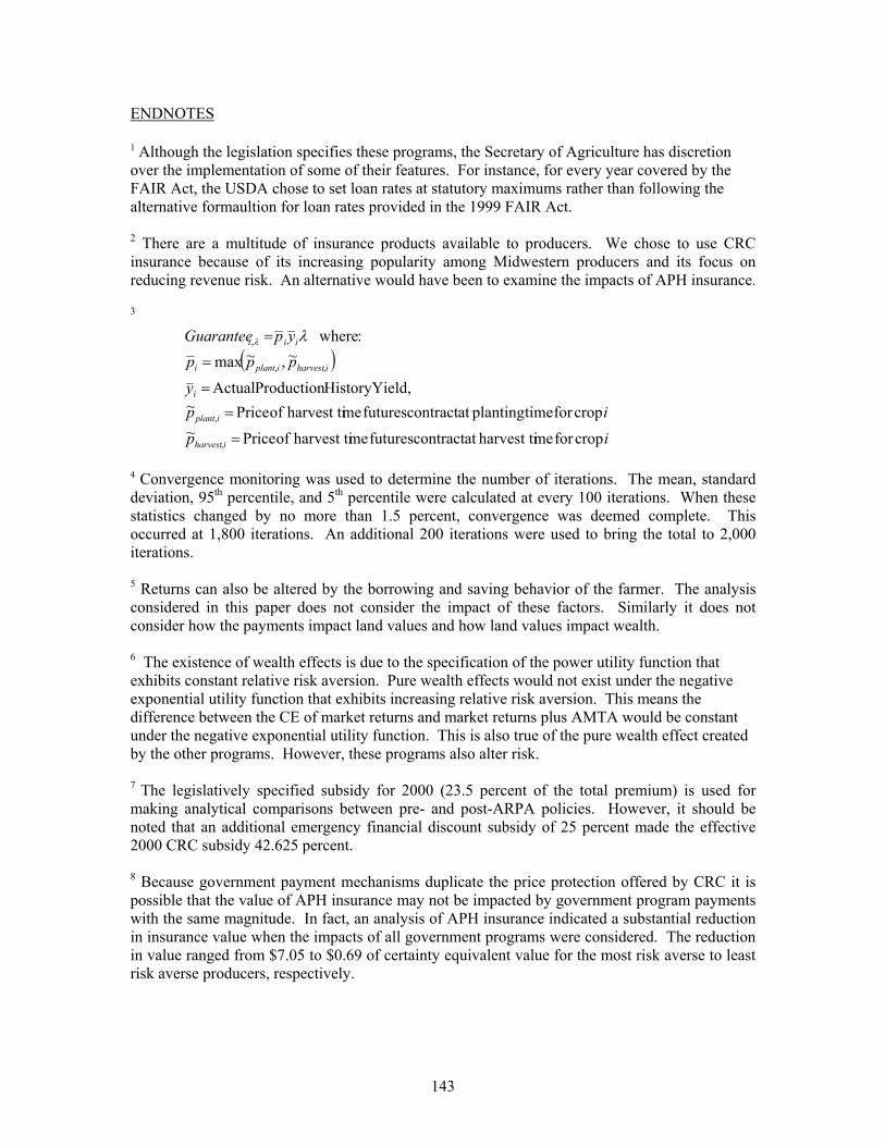
ENDNOTES 1 Although the legislation specifies these programs, the Secretary of Agriculture has discretion over the implementation of some of their features. For instance, for every year covered by the FAIR Act, the USDA chose to set loan rates at statutory maximums rather than following the alternative formaultion for loan rates provided in the 1999 FAIR Act. 2 There are a multitude of insurance products available to producers. We chose to use CRC insurance because of its increasing popularity among Midwestern producers and its focus on reducing revenue risk. An alternative would have been to examine the impacts of APH insurance. 3

( )

ip

ipy

pppypGuarantee

iharvest

iplant

i

iharvestiplanti

iii

cropfor meharvest tiat contract futures meharvest ti of Price ~ cropfor timeplantingat contract futures meharvest ti of Price ~

Yield,History Production Actual

~,~max: where

,

,

,,

,

=

==

=

= λλ

4 Convergence monitoring was used to determine the number of iterations. The mean, standard deviation, 95th percentile, and 5th percentile were calculated at every 100 iterations. When these statistics changed by no more than 1.5 percent, convergence was deemed complete. This occurred at 1,800 iterations. An additional 200 iterations were used to bring the total to 2,000 iterations. 5 Returns can also be altered by the borrowing and saving behavior of the farmer. The analysis considered in this paper does not consider the impact of these factors. Similarly it does not consider how the payments impact land values and how land values impact wealth. 6 The existence of wealth effects is due to the specification of the power utility function that exhibits constant relative risk aversion. Pure wealth effects would not exist under the negative exponential utility function that exhibits increasing relative risk aversion. This means the difference between the CE of market returns and market returns plus AMTA would be constant under the negative exponential utility function. This is also true of the pure wealth effect created by the other programs. However, these programs also alter risk. 7 The legislatively specified subsidy for 2000 (23.5 percent of the total premium) is used for making analytical comparisons between pre- and post-ARPA policies. However, it should be noted that an additional emergency financial discount subsidy of 25 percent made the effective 2000 CRC subsidy 42.625 percent. 8 Because government payment mechanisms duplicate the price protection offered by CRC it is possible that the value of APH insurance may not be impacted by government program payments with the same magnitude. In fact, an analysis of APH insurance indicated a substantial reduction in insurance value when the impacts of all government programs were considered. The reduction in value ranged from $7.05 to $0.69 of certainty equivalent value for the most risk averse to least risk averse producers, respectively.

143

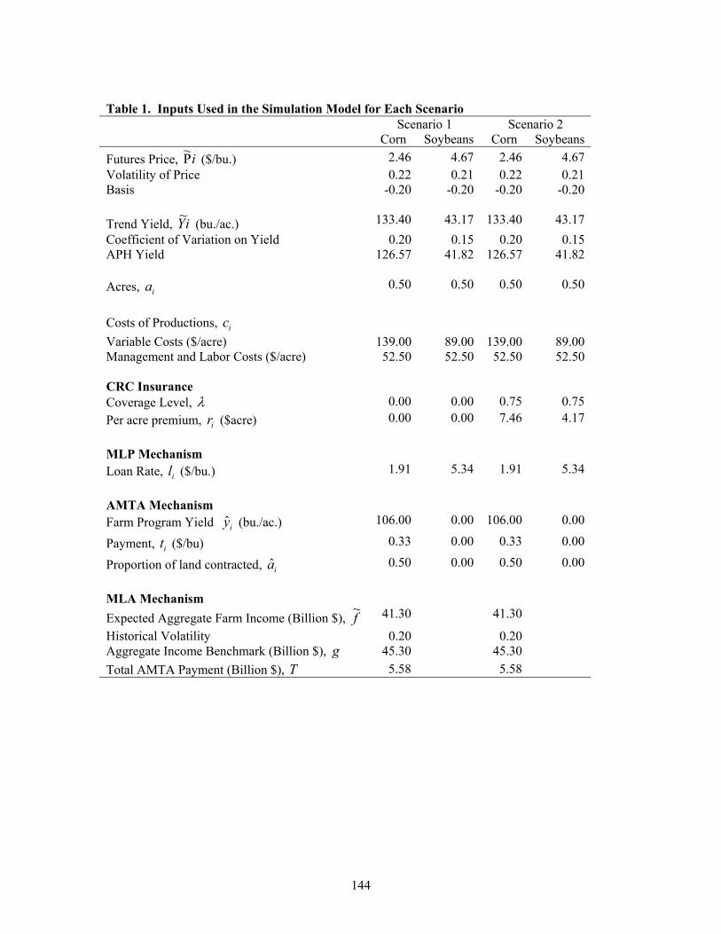
Table 1. Inputs Used in the Simulation Model for Each Scenario Scenario 1 Scenario 2 Corn Soybeans Corn SoybeansFutures Price, iΡ~ ($/bu.) 2.46 4.67 2.46 4.67Volatility of Price 0.22 0.21 0.22 0.21Basis -0.20 -0.20 -0.20 -0.20 Trend Yield, Yi~

(bu./ac.) 133.40 43.17 133.40 43.17Coefficient of Variation on Yield 0.20 0.15 0.20 0.15APH Yield 126.57 41.82 126.57 41.82 Acres, a i

0.50 0.50 0.50 0.50 Costs of Productions, c i

Variable Costs ($/acre) 139.00 89.00 139.00 89.00Management and Labor Costs ($/acre) 52.50 52.50 52.50 52.50 CRC Insurance Coverage Level, λ 0.00 0.00 0.75 0.75Per acre premium, ($acre) ir 0.00 0.00 7.46 4.17 MLP Mechanism Loan Rate, l ($/bu.) i

1.91 5.34 1.91 5.34 AMTA Mechanism Farm Program Yield (bu./ac.) iy 106.00 0.00 106.00 0.00

Payment, ($/bu) it 0.33 0.00 0.33 0.00

Proportion of land contracted, ia 0.50 0.00 0.50 0.00 MLA Mechanism Expected Aggregate Farm Income (Billion $), f~ 41.30 41.30

Historical Volatility 0.20 0.20 Aggregate Income Benchmark (Billion $), g 45.30 45.30 Total AMTA Payment (Billion $), T 5.58 5.58

144

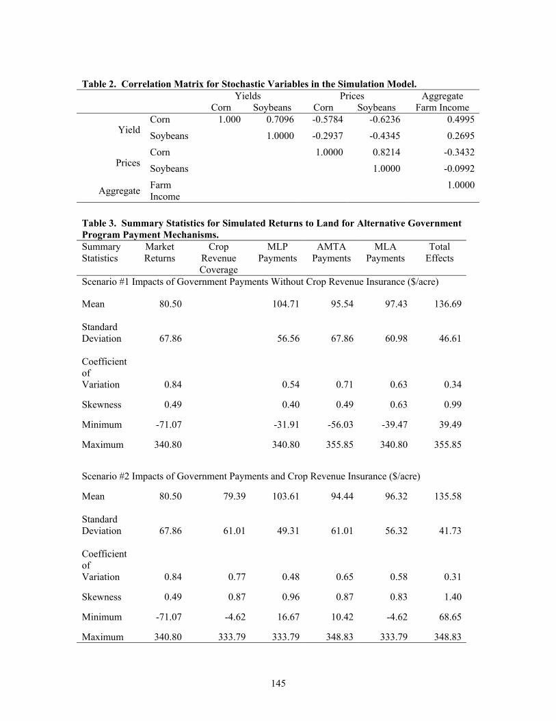
Table 2. Correlation Matrix for Stochastic Variables in the Simulation Model. Yields Prices Aggregate Corn Soybeans Corn Soybeans Farm Income

Corn 1.000 0.7096 -0.5784 -0.6236 0.4995Yield Soybeans 1.0000 -0.2937 -0.4345 0.2695

Corn 1.0000 0.8214 -0.3432Prices Soybeans 1.0000 -0.0992

Aggregate Farm Income

1.0000

Table 3. Summary Statistics for Simulated Returns to Land for Alternative Government Program Payment Mechanisms. Summary Statistics

Market Returns

Crop Revenue Coverage

MLP Payments

AMTA Payments

MLA Payments

Total Effects

Scenario #1 Impacts of Government Payments Without Crop Revenue Insurance ($/acre)

Mean 80.50 104.71 95.54 97.43 136.69 Standard Deviation 67.86 56.56 67.86 60.98 46.61 Coefficient of Variation 0.84 0.54 0.71 0.63 0.34

Skewness 0.49 0.40 0.49 0.63 0.99

Minimum -71.07 -31.91 -56.03 -39.47 39.49

Maximum 340.80 340.80 355.85 340.80 355.85

Scenario #2 Impacts of Government Payments and Crop Revenue Insurance ($/acre)

Mean 80.50 79.39 103.61 94.44 96.32 135.58 Standard Deviation 67.86 61.01 49.31 61.01 56.32 41.73 Coefficient of Variation 0.84 0.77 0.48 0.65 0.58 0.31

Skewness 0.49 0.87 0.96 0.87 0.83 1.40

Minimum -71.07 -4.62 16.67 10.42 -4.62 68.65

Maximum 340.80 333.79 333.79 348.83 333.79 348.83

145

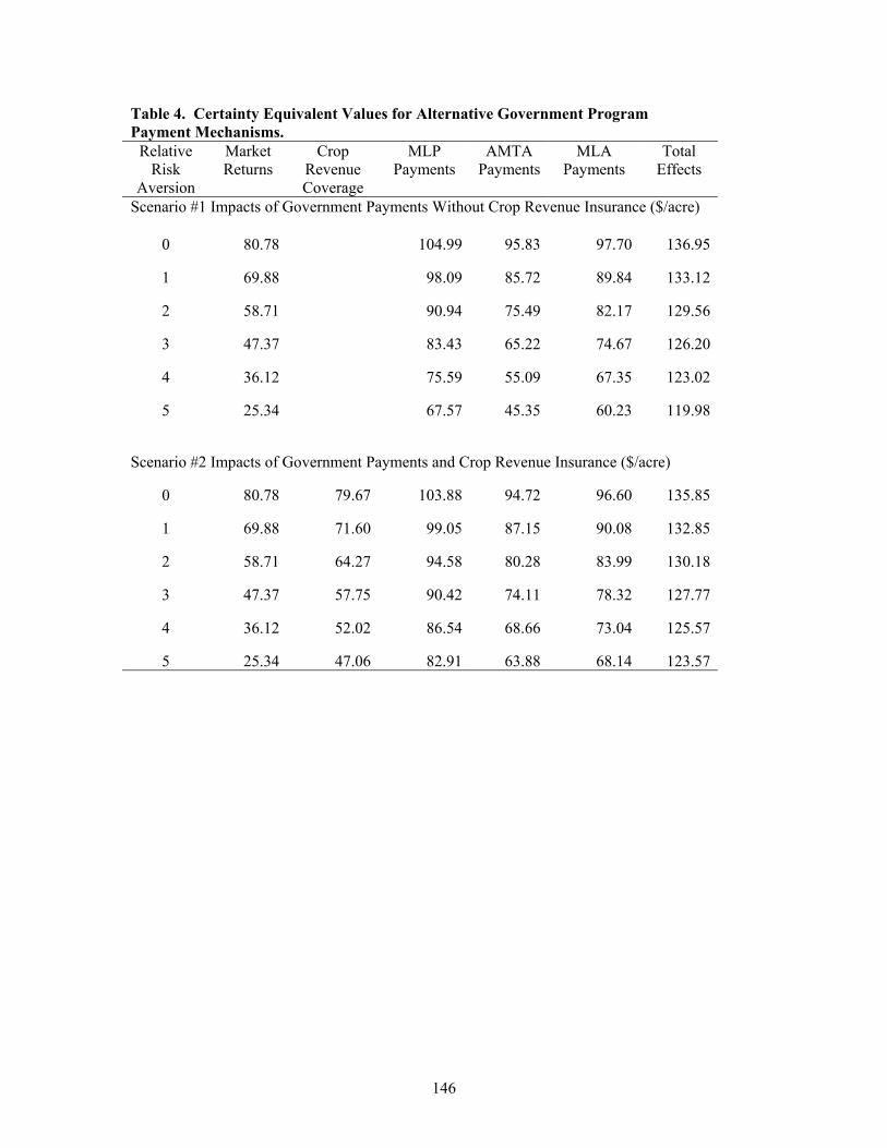
Table 4. Certainty Equivalent Values for Alternative Government Program Payment Mechanisms.

Relative Risk

Aversion

Market Returns

Crop Revenue Coverage

MLP Payments

AMTA Payments

MLA Payments

Total Effects

Scenario #1 Impacts of Government Payments Without Crop Revenue Insurance ($/acre)

0 80.78 104.99 95.83 97.70 136.95

1 69.88 98.09 85.72 89.84 133.12

2 58.71 90.94 75.49 82.17 129.56

3 47.37 83.43 65.22 74.67 126.20

4 36.12 75.59 55.09 67.35 123.02

5 25.34 67.57 45.35 60.23 119.98

Scenario #2 Impacts of Government Payments and Crop Revenue Insurance ($/acre)

0 80.78 79.67 103.88 94.72 96.60 135.85

1 69.88 71.60 99.05 87.15 90.08 132.85

2 58.71 64.27 94.58 80.28 83.99 130.18

3 47.37 57.75 90.42 74.11 78.32 127.77

4 36.12 52.02 86.54 68.66 73.04 125.57

5 25.34 47.06 82.91 63.88 68.14 123.57

146

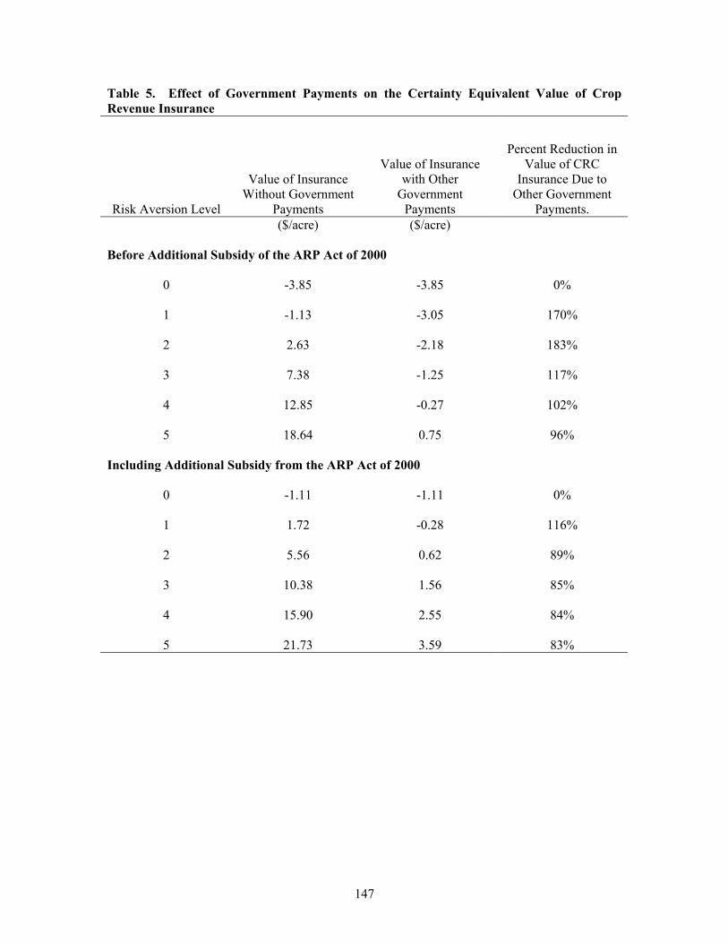
Table 5. Effect of Government Payments on the Certainty Equivalent Value of Crop Revenue Insurance

Risk Aversion Level

Value of Insurance Without Government

Payments

Value of Insurance with Other

Government Payments

Percent Reduction in Value of CRC

Insurance Due to Other Government

Payments. ($/acre) ($/acre)

Before Additional Subsidy of the ARP Act of 2000

0 -3.85 -3.85 0%

1 -1.13 -3.05 170%

2 2.63 -2.18 183%

3 7.38 -1.25 117%

4 12.85 -0.27 102%

5 18.64 0.75 96%

Including Additional Subsidy from the ARP Act of 2000

0 -1.11 -1.11 0%

1 1.72 -0.28 116%

2 5.56 0.62 89%

3 10.38 1.56 85%

4 15.90 2.55 84%

5 21.73 3.59 83%

147

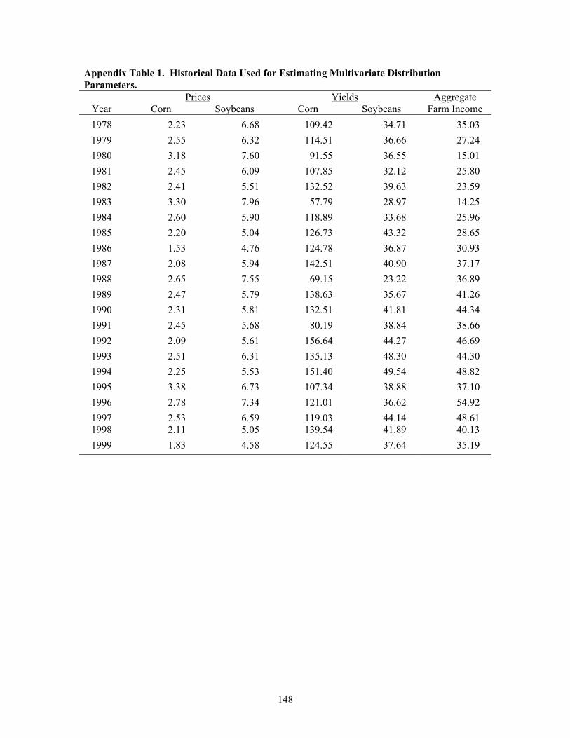
Appendix Table 1. Historical Data Used for Estimating Multivariate Distribution Parameters.

Prices Yields Aggregate Year Corn Soybeans Corn Soybeans Farm Income 1978 2.23 6.68 109.42 34.71 35.03 1979 2.55 6.32 114.51 36.66 27.24 1980 3.18 7.60 91.55 36.55 15.01 1981 2.45 6.09 107.85 32.12 25.80 1982 2.41 5.51 132.52 39.63 23.59 1983 3.30 7.96 57.79 28.97 14.25 1984 2.60 5.90 118.89 33.68 25.96 1985 2.20 5.04 126.73 43.32 28.65 1986 1.53 4.76 124.78 36.87 30.93 1987 2.08 5.94 142.51 40.90 37.17 1988 2.65 7.55 69.15 23.22 36.89 1989 2.47 5.79 138.63 35.67 41.26 1990 2.31 5.81 132.51 41.81 44.34 1991 2.45 5.68 80.19 38.84 38.66 1992 2.09 5.61 156.64 44.27 46.69 1993 2.51 6.31 135.13 48.30 44.30 1994 2.25 5.53 151.40 49.54 48.82 1995 3.38 6.73 107.34 38.88 37.10 1996 2.78 7.34 121.01 36.62 54.92 1997 2.53 6.59 119.03 44.14 48.61 1998 2.11 5.05 139.54 41.89 40.13 1999 1.83 4.58 124.55 37.64 35.19

148