Government Debt and Capital Structure Decisions ...

Government Debt and Capital Structure Decisions:

International Evidence

Irem Demirci, Jennifer Huang, and Clemens Sialm∗

July 16, 2016

Abstract

Our paper investigates the impact of government debt on corporate financing de-cisions. An increase in government debt supply might reduce corporate debt ifinvestors prefer to maintain a relatively stable proportion of debt and equity se-curities. Using data on 40 countries between 1990-2014, we document a negativerelation between government debt and corporate leverage. This relation holds forboth levels and changes of debt, and after controlling for country- and year-fixedeffects as well as country-level controls. Our firm-level analysis shows that theeffect is more prominent when it is easier for corporations to adjust their capitalstructure, for example, for larger and more profitable firms. In order to addresspotential endogeneity issues, we use the introduction of the Euro currency as aquasi-natural experiment that changes the demand for local government bonds incountries adopting the Euro currency. Our findings suggest that government debtcrowds out corporate debt.

JEL Classification: E44, E50, G11, G38

Keywords: Government debt, capital structure, crowding out

∗Irem Demirci is with University of Mannheim, E-mail: [email protected]. JenniferHuang is with Cheung Kong Graduate School of Business, E-mail: [email protected]. ClemensSialm is from the McCombs School of Business, University of Texas at Austin, and is an independentcontractor with AQR Capital Management, Email: [email protected]. We thank Ay-dogan Alti, Kai Li, Vassil Mihov, Stijn Van Nieuwerburgh, Sheridan Titman, Josef Zechner, and seminarparticipants at the Frankfurt School of Finance and Management, the University of Iowa, the Universityof Mannheim, the University of Texas at Austin, and the Vienna University of Economics and Businessfor comments and suggestions.

1 Introduction

Increasing government budget deficits and debt levels have obtained significant at-

tention during the recent financial crisis. However, the impact of government debt on

the economy and on the corporate sector has not been explored much in the financial

economics literature. Our paper investigates whether changes in government debt affect

the financing choices of corporations.

Government debt can crowd out corporate debt if investors in financial markets prefer

to maintain a relatively stable proportion of debt and equity securities in their portfolios.

An increase in government debt will increase the overall supply of debt in the economy.

Households will only be willing to absorb the additional supply if debt securities offer

higher expected returns. To the extent that it is not too costly for firms to deviate from

their target capital structure, they will substitute some of the debt financing using equity

to reduce overall financing costs. Thus, government debt could crowd out corporate debt.

We present a simple model where households can save using equity and debt securi-

ties. Households require a higher return for equity securities, but treat government and

corporate debt as substitutes. Firms finance their projects by issuing both debt and eq-

uity securities, whereas the government is constrained to issue debt securities. The model

shows that an increase in government debt issuances increases the required returns on

debt securities relative to equity securities, and thereby crowds out corporate debt financ-

ing. We also discuss the conditions that lead to differential crowding out effects across

countries facing different institutional structures and across firms with different abilities

to adjust their capital structures.

We empirically test the predictions of our theoretical model using a data set that

covers 40 countries between 1990 and 2014. We find that higher levels of government debt

are associated with lower leverage levels. The results are robust including country- and

year-fixed effects, using alternative specifications based on changes in leverage levels, and

after controlling various time-varying macroeconomic variables. We also obtain consistent

results using a panel of disaggregated firm-level data.

1

We investigate whether the relation between corporate debt and government debt

depends on whether the government debt is financed domestically or internationally.

We hypothesize that the crowding out effect is more pronounced for government debt

purchased by local investors. Consistent with our hypothesis, we find an insignificant

relation between external government debt and local corporate debt. On the other hand,

the coefficient estimates for internal government debt are about twice the estimates for

the total government debt found in our baseline model.

Our international setting also allows us to study the impact of country characteristics

on crowding out effects. We hypothesize that the cost of switching from debt to equity

securities is smaller for firms operating in countries with more developed equity markets

and in countries where bank financing accounts for a small portion of total debt financing.

Our results indicate that a change in government debt only has a significant impact on

corporate debt in countries with relatively large equity markets and in countries where

companies are less dependent on bank financing.

The impact of government debt on capital structure might also differ across firms

within a country for several reasons. First, the debt of some firms (such as large firms

and profitable firms) tends to be less risky and more liquid, so that those securities might

be perceived as closer substitutes for government debt. Second, firms with more financial

flexibility might incur lower costs of switching between debt and equity financing. These

firms might be in a better position to adjust their capital structure in response to shocks

in the supply of government securities. Consistent with our priors, we find that the

crowding out effect is stronger for larger firms and for more profitable firms.

An important concern about the crowding out effect of government debt is that gov-

ernment debt is endogenous. Firms might adjust their capital structure in response to

economic conditions, which are correlated with the supply of government debt.2 We

address this endogeneity concern in multiple ways. As mentioned previously, our spec-

ifications include year-fixed effects that capture the impact of the global business cycle

and additionally control for several country-level macroeconomic variables that capture

2The leverage dynamics of the business cycle is discussed by Hackbarth, Miao, and Morellec (2006),Bharma, Kuehn, and Strebulaev (2010), and Halling, Yu, and Zechner (2015).

2

the local business environment. Furthermore, we only find a crowding out effect for the

portion of government debt that is financed domestically, confirming the postulated seg-

mentation of debt markets. Finally, we use the introduction of the Euro currency as

a quasi-natural experiment to address potential endogeneity concerns. The European

Monetary Union (EMU) facilitated the integration of financial markets in member coun-

tries. Companies and governments in EMU countries gained access to financing from a

substantially broader market and became less dependent on domestic financing sources

after the monetary unification. We find that the sensitivity of corporate leverage to local

government debt decreased significantly for companies incorporated in one of the EMU

countries after the integration, whereas the corresponding sensitivity did not change for

non-EMU countries.

In the corporate finance literature, a significant amount of research is devoted to un-

derstanding how firms make their financing decisions. Many of the empirical studies focus

on the firm-specific determinants of capital structure. For instance, Titman and Wessels

(1988) investigate the empirical validity of theoretical determinants of capital structure

such as asset structure, non-debt tax shields, growth, uniqueness, industry classifica-

tion, size, earnings volatility, and profitability. Besides these firm-specific determinants,

empirical studies show that there are also factors outside the firm, such as industry aver-

age leverage (Welch, 2004 and Frank and Goyal, 2007) and peer firms’ capital structure

(Leary and Roberts, 2014) that shape firms’ capital structure policy. There is also a

growing literature using the variation in the institutional environment across countries

in order to explore the importance of country-specific factors.3 Fan, Titman and Twite

(2012) provide the most extensive analysis of the impact of various institutional factors

such as legal environment, tax policies, and the types of capital providers in the economy

on capital structure. They find that a firm’s capital structure is affected more by the

country in which it is located than by its industry affiliation. Our study contributes

to the literature on country-level determinants of firms’ financing decisions by focusing

3See Booth, Aivazian, Demirguc-Kunt, and Maksimovic (2001), Claessens, Djankov, and Nenova(2001), Demirguc-Kunt and Maksimovic (1996, 1998, 1999), Giannetti (2003), and De Jong, Kabir, andNguyen (2008).

3

attention on government debt.

Greenwood, Hanson, and Stein (2010) develop a model that investigates the impact

of government debt maturity on corporate debt maturity. When the supply of long-term

Treasuries increases relative to the supply of short-term Treasuries, the expected return

on long-term Treasuries increases. Firms absorb this supply shock by issuing short-term

debt to the extent that the expected return differential between long-term and short-

term debt is eliminated. They test the implications of their model using U.S. data and

find a negative relation between corporate debt and government debt maturity. In a

related study, Badoer and James (2015) argue that this gap filling is a more important

determinant of very long-term corporate borrowing than shorter-term borrowing. Using

firm-level corporate debt issuance data, they find that highly rated firms’ issuance of

long-term bonds is inversely related to the proportion of outstanding long-term Treasury

bonds. However, they find little evidence that issuances of short-term corporate bonds

are related to changes in the supply of Treasury bonds. Foley-Fisher, Ramcharan, and Yu

(2014) examine the impact of the Federal Reserve’s Maturity Extension Program (MEP)

on the firm financial constraints. The MEP was intended to put downward pressure

on long-term interest rates, to lower borrowing costs, and to increase the amount of

credit available to firms and households. They find that firms that rely on long-term

debt issued more long-term debt during the MEP’s implementation. Furthermore, such

firms enjoyed increases in investment and employment during the MEP relative to other

periods, suggesting that the MEP affected real economic activity.

Krishnamurthy and Vissing-Jorgensen (2012) argue that similar to money, Treasury

securities also have liquidity and safety attributes, and an increase in the supply of govern-

ment securities decreases the relative value of those attributes in the market. Consistent

with this hypothesis, they find that a one standard deviation decrease in the Treasury

supply reduces Baa-Treasury spreads by 79 basis points. Furthermore, by studying pairs

of assets with similar liquidity but different safety or with similar safety but different

liquidity, they show that changes in Treasury supply affect both the safety and liquidity

premia.

4

Our paper is most related to Graham, Leary and Roberts (2014), who investigate

the government crowding out of corporate debt using unique long-term U.S. data from

1920-2012. They find a robust negative relationship between government leverage and

corporate leverage. Their analysis of the portfolios of different financial intermediaries,

such as commercial banks, insurance companies and pension funds, suggests that financial

intermediaries respond to increased government borrowing by increasing their holdings of

government debt and by reducing their holdings of corporate debt. Our paper contributes

to the literature by investigating the crowding out effect between government and corpo-

rate debt using a cross-country sample. Using international data allows us to benefit from

a larger variation of changes in government debt and to control for year effects, country

effects, and time-varying macroeconomic factors. Furthermore, our empirical analysis of

the Euro integration also helps to mitigate potential endogeneity concerns.

The remainder of the paper is organized as follows: Section 2 presents a simple model

that formalizes the main ideas discussed in the Introduction. Section 3 describes the

data and reports the summary statistics. Section 4 presents the country-level empirical

analysis and robustness tests. Section 5 analyzes the crowding out effect using firm-level

data. Section 6 studies how the relation between corporate leverage and government debt

changes around the formation of the EMU. We conclude in the final section.

2 The Model

We describe in this section a simple model that illustrates crowding out effects. Our

model includes three economic agents: households who save, firms who require financing

to fund their projects, and the government.

2.1 Household’s Optimization Problem

The representative household is endowed with an initial wealth of W , and decides

how much to allocate to debt and equity securities in order to maximize the utility from

5

next period’s consumption:

maxwD,wG

U [(1− wD − wG)(1 + rE)W + wD(1 + rD)W + wG(1 + rG)W + v(ρwD + wG)W ] ,

where rE, rD, and rG are deterministic returns on equity, corporate debt, and government

debt.4 The portfolio weights wD and wG denote the fractions of initial wealth invested

in corporate and government debt securities, respectively. The rest of the portfolio,

1− wD − wG is invested in corporate equity.

Similar to the model in Krishnamurthy and Vissing-Jorgensen (2015), the household

obtains additional utility v from holding safer debt-like assets. We assume that v′(·) > 0

and v′′(·) < 0. Finally, ρ captures the substitutability between corporate and government

debt (ρ ∈ (0, 1]). As ρ approaches one, households treat corporate debt as a perfect

substitute for government debt.5

The household’s first order conditions imply:

v′(ρwD + wG) = rE − rG, (1)

ρv′(ρwD + wG) = rE − rD. (2)

We do not explicitly model risk and the associated risk premium for equity in our model.

The spread between the return on equity and debt securities captures in a reduced-form

the preference for safer assets from investors. Combining these two equations yields the

following equation for the spread between corporate debt and government debt:

rD − rG = (1− ρ)v′(ρwD + wG). (3)

As corporate debt becomes a perfect substitute for government debt (i.e. as ρ→ 1), the

spread between corporate debt and government debt shrinks towards zero.

4We ignore risk on corporate equity for simplicity, as our focus is the tradeoff between corporate andgovernment debts.

5The utility v for “safer” asset is similar to the preference for “extremely safe” assets in Krishnamurthyand Vissing-Jorgensen (2015). They model the preference for bank deposits plus Treasury bonds. Ourparameter ρ allows us to differentiate between investors’ preferences for “extremely safe” (e.g. Treasurybonds) and “safe” assets (e.g. corporate bonds) relative to equity.

6

2.2 Firm’s Optimization Problem

Firms have projects that require an investment of K in the first period and produce

an output of f(K) in the second period. The total investment K is financed by equity

and debt. The target capital structure is to have λ fraction of total capital financed by

debt. Firms incur quadratic costs for any deviation from this target. These costs capture

the impact of various market frictions, such as taxes, agency costs, and other financing

costs. Each firm takes as a given the external financing costs rD and rE, and chooses the

leverage ratio d to maximize total output net of financing and deviation costs:

maxd

f(K)− d(1 + rD)K − (1− d)(1 + rE)K − θ

2 (d− λ)2 K,

where

d = D

K.

The firm’s first-order condition is as follows:

θ (d− λ) = rE − rD. (4)

The firm chooses the leverage ratio d to take advantage of the rate differential rE − rD.

This rate differential captures external capital market conditions that are unrelated to

the firm’s specific risk. The higher the cost of deviation θ, the less the firm deviates from

its target capital structure λ.

2.3 Market Equilibrium

The following equilibrium condition follows from equations (2) and (4):

r∗E − r∗D = θ(d∗ − λ) = ρv′(ρw∗D + wG). (5)

The equilibrium corporate debt level d∗ is determined by households’ preference for safer

debt-like instruments and the cost for firms to deviate from their target debt levels. The

target λ captures in a reduced-form way the optimal tradeoff at the firm level, before

accounting for the capital market imperfection in which households have a preference for

7

safer assets. This preference leads to a lower cost of corporate debt relative to equity. As

a result, firms increase their debt level relative to the original target level λ.6

In equilibrium, equity and debt markets clear such that:7

W = E +D +G = K +G.

Therefore, an increase in government debt is absorbed by the household sector and shrinks

the corporate sector by the same amount.8 Figure 1 depicts the debt-to-capital ratio in

equilibrium for the case when v(·) is a logarithmic function (i.e., v(x) = log(1 + x)). The

horizontal axis shows different leverage levels d and the vertical axis shows the equity

premium rE − rD. The preferences of households for debt securities are captured by

the downward-sloping curve ρv′(ρd(1 − wG) + wG). As debt securities become more

abundant, households do not require a large equity premium to be indifferent between

holding equity and debt securities. The upward-sloping line θ(d−λ) captures the capital

structure preferences of firms. At a leverage ratio of d = λ, the frictions of debt financing

would be minimized. However, due to the household’s preference for debt-like securities,

the return that households demand for holding equity is higher than debt at d = λ by

an amount of ρv′(ρλ(1 − wG) + wG). Therefore, the firm increases its leverage from

the target level λ to d∗ where the marginal cost of debt financing equals the marginal

benefit of holding debt for the household. The figure shows that the equilibrium level of

debt-to-capital (d∗) corresponds to a positive equity premium.

<Figure 1 about here>

6An alternative way of formulating the household’s problem is to assume an optimal portfolio sharefor debt securities and quadratic costs of deviating from this optimum. All of the implications that wederive using our current model survive as long as the optimal portfolio share of debt for the householdis greater than the firm’s target leverage ratio.

7Substituting the market clearing condition in the definitions of wD, wG and d, we obtain the followingrelationship between the household’s portfolio share of debt and the firm’s leverage ratio:

w∗D = d∗(1− wG). (6)

8This assumption is for simplification and our results are not driven by this assumption since we derivethe optimal leverage ratio rather than optimal debt level in equilibrium. Our implications continue tohold if we assume that some or all of the increase in government debt is transferred to the households,thus corporate investment does not shrink at all or is reduced less than the increase in government debt.

8

2.4 Impact of Government Debt

We now consider the impact of government debt on the corporate leverage ratio. We

have the following result.

Implication 1: Given households’ preference for debt-like instruments and financing

frictions of the corporate sector, an increase in government debt leads to a lower corporate

leverage ratio. Furthermore, it reduces both the spread between equity and corporate debt

and the spread between corporate and government debt.

The detailed proof is in the appendix. Figure 2 shows how the introduction of govern-

ment debt affects the equilibrium in financial markets. The introduction of government

debt shifts the household’s marginal utility curve (v′) to the left, since the household

now has a larger share of debt securities for a given portfolio share of corporate debt.

The introduction of government debt reduces the equity premium as well as the optimal

amount of corporate debt.


2.5 Countries with Different Financing Frictions

Next, we investigate whether the crowding out effect differs between countries with

different financing frictions. We use the cost of deviating from optimal capital structure

(θ) as a measure of financing frictions. In a country with a more developed equity market

and lower financing frictions, it is less costly for firms to deviate from their target capital

structure.

To simplify notation we abbreviate the equity premium as: EP = rE − rD. It can be

shown that the following inequality holds9:

θH = EP ∗H − EP ∗∗Hd∗H − d∗∗H

>EP ∗L − EP ∗∗Ld∗L − d∗∗L

= θL. (7)

Implication 2: Given an increase in government debt, countries with higher financing

9See the appendix for the proof.

9

frictions experience a smaller reduction in corporate debt. However, these countries ex-

perience a larger drop in both the spread between equity and corporate debt and the spread

between corporate and government debt.

Figure 3 compares the change in the equilibrium level of debt for countries with high

(θH) and low (θL) financial frictions. We compare the equilibrium outcomes without a

government sector (denoted with one asterisk) and with a government sector (denoted

with two asterisks).


When financing frictions are high, the introduction of a government sector generates

stronger price responses and weaker quantity responses compared to the case with low

adjustment costs. This outcome is intuitive because firms are not as flexible to adjust

their leverage levels in environments with more substantial frictions. Without quantity

adjustment, the price impact is larger. Since our empirical tests focus only on the quantity

responses, we underestimate the impact of government debt for countries with higher

frictions.

2.6 Heterogeneity in Firm Composition

We also analyze the model’s implications for two firms that are incorporated in the

same country, but their corporate debts have different levels of substitutability with

government debt due to different credit quality or liquidity. For simplicity we assume the

two firms have the same optimal target leverage (λi = λ) and the same financing frictions

(θi = θ).10

10We solve for the case where firms have different financing frictions but the same level of substi-tutability in the Appendix.

10

The household’s problem is summarized as follows

maxwEL

,wDL,wDH

,wGU [(1− wEL

− wDL− wDH

− wG)(1 + rEH)W + wEL

(1 + rEL)W

+ wDL(1 + rDL

)W + wDH(1 + rDH

)W + wG(1 + rG)W

+ v (ρLwDL+ ρHwDH

+ wG)W ],

where wDiand wEi

are the fractions of initial wealth invested into debt and equity of

firm i ∈ {L,H}. The following equations are derived from the household’s first order

conditions

rEi− rG = v′(ρLwDL

+ ρHwDH+ wG) (8)

rEi− rDi

= ρiv′(ρLwDL

+ ρHwDH+ wG). (9)

In equilibrium, the representative investor is indifferent between investing into the equities

of high-ρ and the low-ρ firm such that r∗EL= r∗EH

. Consequently, the difference between

the returns on debt securities supplied by the high-ρ and the low-ρ firm are determined

by the difference between their contributions to marginal utility. Each entrepreneur

i ∈ {L,H} solves the following problem:

maxdi

f(Ki)− di(1 + rDi)K − (1− di)(1 + rEi

)K − θ

2 (di − λi)2 Ki.

We derive the following first order condition for entrepreneur i’s problem

rEi− rDi

= θ (di − λi) . (10)

In this case, the equilibrium condition is given by

ρiv′ (ρLwDL

+ ρHwDH+ wG) = θ (d∗i − λ) (11)

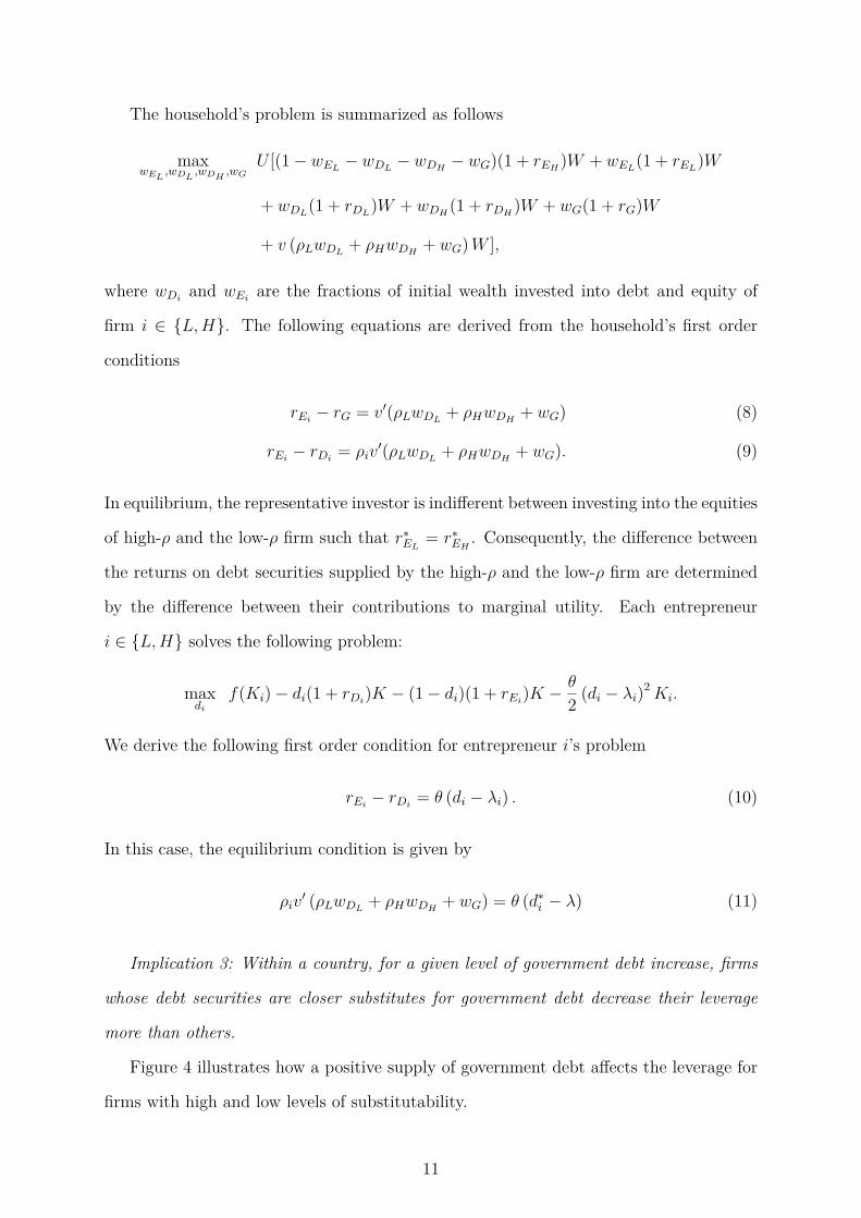
Implication 3: Within a country, for a given level of government debt increase, firms

whose debt securities are closer substitutes for government debt decrease their leverage

more than others.

Figure 4 illustrates how a positive supply of government debt affects the leverage for

firms with high and low levels of substitutability.

11


3 Data and Summary Statistics

This section describes the data sources and summarizes the main variables used in

our empirical analysis.

3.1 Data

We obtain firm-level accounting data from Compustat Global and Compustat North

America, and firm-level market data from Compustat Global Security Daily. The main

variable of interest is the total government debt-to-GDP ratio, which we obtain from

the World Economic Outlook (WEO) database available through the IMF11. For other

country-level variables, we use data from the World Bank, IMF and the ECB. To ensure

that the country-level variables are consistently defined over time, for each country and

variable, we use the data source that provides us with the longest series. We obtain the

data on sovereign debt defaults and restructuring episodes from Carmen M. Reinhart

and Kenneth S. Rogoff’s webpage.12 The website offers the longest historical annual

government debt data from as early as 1692 for the UK and 1719 for Sweden to 2010 for

70 countries.

Our sample covers the period between 1990 and 2014, and the first year of the sample

is determined by the availability of the firm-level and country-level data which vary across

countries. Observations with missing and/or negative book value of assets are dropped

from the sample. We exclude financial (6000-6999), public (9000-9999) and utility (4900-

4999) firms. Since we focus on the time-series variation in corporate and public debt, each

firm is required to have data on book leverage, lagged firm-level controls, as well as lagged

values of government debt, GDP per capita, inflation, S&P index level, unemployment,

11The WEO series are not available for the earlier periods of our sample for some countries. For thosecountries with short series we use government debt data from the central banks whenever available orother sources such as World Bank. Those countries are Ireland, Israel, Peru, South Africa, and the US.

12http://www.reinhartandrogoff.com/

12

http://www.reinhartandrogoff.com/

and nominal exchange rate. We also exclude country-year observations with less than

ten firms.

Our sample includes 16 country-year observations in which we observe a domestic or

external sovereign debt default or restructuring event. These events are associated with

large decreases and increases in government debt-to-GDP ratios that might result from

significant devaluations of the local currency and debt forgiveness. While our exchange

rate captures such devaluations, our macro controls cannot account for debt forgiveness.

We exclude these 16 country-year observations from our analysis. The final sample con-

sists of 38,740 firms from 40 countries with a total of 344,132 firm-year observations and

812 country-year observations.

Table 1 shows the distribution of countries in our sample. The sample includes firms

from different parts of the world, mainly Europe, Asia, North America, and South Amer-

ica. Hong Kong has the shortest time series that mainly results from government debt

not being available in the earlier periods of the sample. The U.S., the U.K., and Japan

are the countries with the highest number of firm-year observations.

<Table 1 about here>

3.2 Summary Statistics

We use four leverage measures for our firm-level analyses. First, we define the tradi-

tional leverage measures, Book Leverage and Market Leverage, which are total debt over

book value of assets and total debt over market value of assets, respectively. Net Book

Leverage is defined as book leverage net of cash and short-term investments. The last

measure, Debt-to-Capital Ratio, is proposed by Welch (2011), and is defined as the book

value of debt divided by debt plus the book value of equity. The book value of total assets

includes the value of non-financial liabilities such as trade credit. Therefore, an increase

in accounts receivable causes a decrease in the book leverage, even if total debt of the firm

stays constant. The last definition of leverage is not affected by changes in non-financial

liabilities. The country-level variables follow firm-level definitions, and are calculated by

13

aggregating the values in the numerator and the denominator over all firms in a given

year and country. All ratio variables, including leverage measures, are winsorized at the

1% level.

Table 2 reports country averages for corporate leverage and macroeconomic variables.

While, on average, firms in Hong Kong have the lowest leverage ratio, firms in Portugal

have the highest corporate leverage in our sample. Belgium, Greece, Italy, and Japan are

countries with an average government debt-to-GDP ratio exceeding 100%. Chile, Hong

Kong, and Russia have the lowest average government debt-to-GDP ratios that are all

below 20%.


Besides our main country-level debt variables, we also control for other country char-

acteristics.13 Our main specification includes GDP per capita, the level of inflation, the

level of the equity index, the unemployment rate, and the exchange rate. The natural

logarithm of GDP per Capita is measured in current U.S. dollars, whereas Inflation is

defined as the natural logarithm of the level of consumer price index. In order to account

for the movements in the stock market, we convert each country’s return on its S&P

Global Equity Index into a variable that tracks the index level assuming that the base

year is the first year in the sample, and include the natural logarithm of this index in our

regressions. Unemployment is the number of unemployed as a percentage of the potential

labor force. Although, we use year-fixed effects in all specifications, we cannot control

for economic downturns specific to each country, which makes the unemployment rate

an important variable to include in the analysis. Finally, Nominal Exchange Rate is the

value of the local currency relative to one U.S. dollar calculated as an annual rate based

on monthly averages, and we control for its natural logarithm in all our analysis.

We also compute additional firm-level variables that have been shown to relate to

corporate leverage (Rajan and Zingales,1995, Baker and Wurgler, 2002, Frank and Goyal,

2003, and Lemmon, Roberts and Zender, 2008). Tangibility is defined as the ratio between13See Korajczyk and Levy (2003) for the macroeconomic determinants of capital structure.

14

the value of property, plant, and equipment (PPE) and total assets. We use the book

value of total assets (Assets) to account for the impact of firm size on leverage. The

return on assets (ROA) is defined as operating income scaled by total assets. Finally,

Market-to-Book Ratio is defined as the ratio between the market value of total assets and

the book value of the firm. We use Compustat currency exchange rate data in order to

convert non-ratio variables into U.S. dollars. Detailed variable definitions are given in

the Appendix.

Panels A and B of Table 3 report the summary statistics for country- and firm-

level variables, respectively. Government debt-to-GDP has a mean of 58.3% and an

interquartile range of 37.2% and 72.5%. On average, the GDP per Capita is $16,075, and

the average unemployment rate is about 7.4%. Panel A of Table 3 shows that the ratio

between corporate debt and corporate total assets has a mean (median) of 28.3% (27.7%)

and a standard deviation of 6.5%. On average, book leverage net of cash is 17.8% with

a standard deviation of 8.1%. Since it is normalized by the book value of total capital

rather than total assets, the Debt-to-Capital Ratio is higher than the Book Leverage, with

a mean (median) of 42.3% (42%). Finally, the Market Leverage has an average of 19.5%

and a median of 18.5%.


Panel B reports the summary statistics for firm-level variables. On average, Book

Leverage, Net Book Leverage, Debt-to-Capital and Market Leverage are 21.7%, 5%, 29.7%

and 18.1%, respectively. Consistent with the capital structure literature, we find a sig-

nificant variation in the tangibility of firms. The mean tangibility equals 30.5% with an

interquartile range of [11.3%, 44.7%]. Most firms in our sample are profitable, as cap-

tured by the 4.2% positive mean ROA. Finally, the median firm’s market value exceeds

the book value by 23.2%.

15

4 Country-Level Analysis

This section presents the results of our empirical analyses using the country panel

where we aggregate firm-level variables by year and country. One potential caveat of

this approach is that the composition of the aggregated sample might change as firms go

public or are delisted from security exchanges. To alleviate this problem, we report the

results from firm-level specifications in Section 5.

4.1 Baseline Specification

Our baseline specification relates the country-level corporate debt to government debt-

to-GDP ratio and additional macro variables. More specifically, we estimate the following

regression equation:

Leveragej,t = β0 + β1Government Debt-to-GDPj,t−1

+ β2Xj,t−1 + β3Yj,t−1 + uj + δt + εj,t.

(12)

Equation (12) is estimated separately for four different definitions of Leveragej,t,

namely book leverage, book leverage net of cash, market leverage, and total debt divided

by debt plus equity. Government Debt-to -GDPj,t−1 is total government debt as a percent-

age of GDP in country j; Xj,t−1 denotes macro variables, including the natural logarithm

of GDP per capita, inflation, the level of the equity index, the unemployment and the

exchange rate; Yj,t−1 denotes aggregated values of traditional determinants of leverage

that are frequently used in capital structure studies, mainly tangibility, size, profitability,

and the market-to-book ratio. Finally, uj and δt denote country- and year-fixed effects,

respectively. Year-fixed effects account for worldwide events such as the recent financial

crisis, and country-fixed effects control for time-invariant country characteristics.

Panel A of Table 4 reports the results for the levels specification. The standard

errors are clustered at the country level and t-statistics are reported in parentheses. The

results indicate a negative relationship between government debt and aggregate corporate

leverage. A 10 percentage point increase in government debt relative to GDP reduces

16

book leverage (market leverage) by about 0.75 (0.56) percentage points. Government

debt is also negatively correlated with net book leverage (debt-to-capital ratio): a 10

percentage point increase in government debt-to-GDP is associated with a 0.86 (0.96)

percentage point decrease in net book leverage (debt-to-capital ratio). The unemployment

rate and the exchange rate are significant determinants of corporate leverage. Also, the

profitability is significantly related to the aggregate leverage.


We repeat our analysis for the subsample of countries that are members of the

OECD.14 Panel B of Table 4 reports the fixed effects regression results for the 25 OECD

countries. Results are similar to those reported for the whole sample with the relation-

ship between government debt and corporate debt being slightly stronger for developed

countries.

A second method for analyzing the time-series relationship between corporate debt

and government debt is to estimate equation (12) in first differences:

∆Leveragej,t,t−1 = β0 + β1∆Government Debt-to-GDPj,t−1,t−2

+ β2∆Xj,t−1,t−2 + β3∆Yj,t−1,t−2 + δt + εj,t.

(13)

Panel A of Table 5 reports the results for country-level first difference regressions. The

coefficient estimates for the government debt-to-GDP ratio are all negative for our four

different leverage measures such that corporate leverage decreases significantly following

an increase in government debt. For example, a 10% increase in government debt-to-GDP

is associated with a 0.68% (0.59%) decrease in firm book leverage (market leverage) in the

subsequent year. Similarly, net book leverage and debt-to-capital ratio change by -0.77%

and -1.08%, respectively. The economic magnitude in the first difference specification is

14Those countries are: Austria, Australia, Belgium, Canada, Denmark, Germany, Finland, France,Greece, Ireland, Italy, Japan, South Korea, Mexico, Netherlands, Norway, New Zealand, Poland, Portu-gal, Spain, Sweden, Switzerland, Turkey, US, UK. Since they became members in 2010, Chile and Israelare not included in the OECD sample. Note that only two OECD countries, Turkey and Greece, expe-rienced a default or a restructuring in our sample. Therefore, only two observations in this subsampleare dropped due to such episodes.

17

very similar to the magnitude in the level specification. Note that changes in GDP per

capita, ROA, and the market-to-book ratio are typically significantly related to changes

in corporate debt. Overall, our findings suggest that there is a negative relation between

firm leverage and government debt supply.


We repeat our first difference analysis for the OECD countries as we did for the levels

specification in Table 4. Table 5 Panel B reports the results. Consistent with the fixed

effects regression results, the coefficient estimates for the OECD subsample are similar

to those estimated for the whole sample.

4.2 External Debt

Our government debt variable includes both external and domestic government debt.

Consequently, there can be cases where an increase in the supply of government debt is

absorbed by foreign investors or international financial institutions such as the IMF. In

the latter case, we do not expect the change in government debt to have any impact on

corporate leverage as long as the stock of local government debt stays constant. There

are two potential channels through which corporate debt can be affected from changes

in foreign demand for government bonds. First, holding the change in total government

debt constant, a larger fraction of a debt issue is absorbed by foreign investors, leaving

more local funds available for corporations. Second, the increase in foreign demand

for government debt can crowd out foreign investment into corporations. The latter

effect would be more prominent in those countries where external private debt is a more

important source of debt financing than domestic private debt. According to the IMF

(2015), over the period between 2003 and 2014, foreign bank lending to the private sector

in emerging markets stayed below 8% of total debt, whereas domestic bank lending was

above 78%. Although, bond financing has doubled from 8% to 16% since 2008, domestic

bank lending is still the main source of debt financing in emerging markets.

18

In Table 6, we repeat our baseline analysis by replacing Government debt-to-GDP

with Domestic Government Debt and External Government Debt measured in percent

of GDP. Domestic Government Debt is calculated by subtracting external government

debt from total government debt outstanding. The results are reported for both fixed

effects and first difference specifications. The economic magnitude of the estimate for

the coefficient of internal government debt is twice the estimate for total government

debt reported in Table 4. Furthermore, the coefficient estimate for external debt is

insignificant suggesting that the negative relationship between corporate leverage and

government leverage is driven by domestic public debt rather than external debt.15


4.3 An Alternative Specification

One possible concern about using the government debt-to-GDP ratio as the indepen-

dent variable is that the relationship between corporate leverage and government debt

could be driven by changes in GDP rather than changes in the amount of government debt

outstanding. In order to eliminate this concern, we estimate an alternative specification.

More specifically, we regress the natural logarithm of the dollar value of corporate debt

on the natural logarithm of the dollar value of lagged government debt. The coefficients

in this specification can be interpreted as the elasticities of corporate debt in response to

changes in government debt.

Table 7 reports the estimation results which confirm our findings in Table 4 and Table

5. Results are consistent with our previous findings. For instance, in the fixed effects

regressions a one standard deviation (1.590) increase in the natural logarithm of govern-

ment debt is associated with a 0.144 standard deviation decrease in the natural logarithm

15The correlation between the levels (first differences) of external and internal government debt is0.214 (0.376). Although, they are statistically significant, correlation coefficients are not large enough toraise multicollinearity concerns. Furthermore, the variance inflation factors associated with the changesin external and internal government debt are both close to one.

19

of corporate debt. We obtain similar results for the first difference specification.16


4.4 Country Characteristics and Crowding Out

We also investigate the cross-country variation in the crowding out effect. We hypoth-

esize that in countries where financial markets are more developed, it is less costly for

firms to adjust their capital structure. Consequently, we expect firms in such countries

to find it easier to change their capital structure when government debt changes.

To investigate the cross-country variation in crowding out, we use three proxies,

namely, size of the equity market, bank dependence of the private sector and stock

turnover ratio. Market Capitalization is total market value of pubic firms as a percent of

GDP. Bank Dependence is the amount of bank credit extended to the private sector (%

total credit) which proxies for the dependence of corporations on banks. Stock Turnover

Ratio is the value of domestic shares traded divided by their market capitalization which

captures the liquidity of an equity market. In each year, we split the sample into three

equally-sized groups based on previous year’s Market Capitalization, Bank Dependence

and Stock Turnover Ratio.

Panel A of Table 8 reports the first difference estimation results for the three subsam-

ples based on the size of the equity market. While the coefficient estimates for change in

government debt-to-GDP are in general negative, they are only statistically significant

and are the largest in magnitude for countries with a large equity market. Panels B and

C report the results for the subsamples based on the fraction of bank credit and the

stock turnover ratio. The results show that the crowding out effect is more prominent in

countries with a less bank-dependent private sector and a high stock turnover ratio.


16In order to ensure that the results are not driven by a single country in our sample, we repeat thefixed effects and first difference regressions in Table 4 and Table 5 by dropping one country at a timefrom our sample. Our results are robust to these subsamples.

20

5 Firm-Level Analysis

In this section, we estimate our baseline model at the firm level. Table 9 reports the

estimation results for firm fixed effects and the first difference specification. The results

show that the coefficient estimates for the firm-level controls have the signs consistent

with the literature. While tangibility and size have a positive impact on leverage, prof-

itable firms and those with high market-to-book ratios have lower leverage. We obtain a

negative relation between the level of government debt and firm leverage levels for all four

leverage measures. The coefficient estimates imply that a 10 percentage point increase in

government debt relative to GDP reduces firm leverage by 0.48-0.77 percentage points.

Similarly, the coefficient estimates from the first difference specification are consistent

with our previous findings. A 10 percentage point change in government debt relative to

GDP reduces firm leverage by 0.73-0.99 percentage points.


We conduct several robustness checks for our firm-level analysis which we report in the

Appendix. First, as an alternative to our baseline specification, we repeat our firm-level

analysis using the natural logarithms of government debt and corporate debt in dollars.

Table A2 shows that the results are robust to this alternative definition.

We also differentiate between domestic and external government debt at the firm level.

Results are reported in Table A3, which confirm the findings from country-level analysis

such that external debt is not significantly related to corporate leverage and there is a

negative relationship between domestic debt and leverage.

We also investigate whether the negative impact of government debt on corporate

leverage is specific to long-term or short-term corporate debt. In Table A4, we repeat our

main analysis for Long-Term Debt defined as long-term debt that matures in more than

one year divided by total assets, and for Short-term Debt defined as the ratio of debt in

current liabilities to total assets. Results indicate that the negative relationship holds for

both long-term and short-term corporate debt.

21

One advantage of our firm-level analysis is that it allows us to investigate the impact

of firm characteristics on the crowding out effect, as discussed in our theoretical model.

The impact of government debt on capital structure might differ across firms for two

reasons. First, some types of corporate debt are closer substitutes to government debt

than others. For example, bonds issued by larger firms might be more liquidly traded.

Similarly, more profitable firms tend to have lower default risk, which makes their debt a

better substitute for government debt. Thus, the crowding out effect should be stronger

for large and profitable firms. Second, firms with more financial flexibility incur lower

costs of switching between debt and other sources of financing. These firms are in a better

position to adjust their capital structure in response to shifts in demand. For example,

larger firms are more flexible in their choices between debt and equity financing, since they

are potentially less subject to asymmetric information problems. In contrast, high equity

issuance costs or borrowing costs might prevent small firms from drastically changing

their method of financing. Similarly, more profitable firms face lower costs in adjusting

their capital structure because they have the flexibility of first drawing down their internal

funds before tapping the external capital market. Moreover, they may face a lower cost of

switching between debt and equity financing. Therefore, both the substitution effect and

the adjustment cost effect suggest that larger and more profitable firms should respond

more to government debt changes.

In columns (1)-(4) of Table 10 we interact government debt-to-GDP ratio with indi-

cator variables for firm size. More specifically, we split firms into three terciles in each

year and each country by total book value of assets. Consistent with our prior, we find

that the crowding out effect is significantly higher for large firms than for small firms.


Similarly, we expect profitable firms to respond more to changes in government debt.

Such firms are more likely to have high retained earnings that they can use towards in-

vestment without any need for external financing. Columns (5)-(8) of Table 10 report the

results for profitability interactions, where the dummy variable ROA Tercile 3 indicates

22

that the firm’s lagged ROA is in the highest tercile of its country distribution in a given

year. The results show that the crowding out effect is more significant for profitable firms.

Overall, we find consistent evidence with our model’s implications such that government

crowding out is more prominent for firms that are financially less constrained.

6 Euro-Area Integration

Although we control in our baseline analysis for time-invariant country characteristics,

various macroeconomic controls, and year-fixed effects that account for worldwide events

such as the financial crisis, endogeneity concerns might remain. In this section, we address

this concern by using the integration of the bond market in the European Monetary

Union (EMU) as a quasi-natural experiment. Since the second half of the 1990s, the

degree of integration in various European financial markets has significantly increased

(ECB, 2006). The effect has especially been prominent in government and corporate

bond markets (Pagano and Von Thadden, 2004 and ECB, 2006).

Coeurdacier and Martin (2007) argue that in theory, the monetary integration can

have opposing effects on the holdings of Euro assets by countries in the Euro zone. For

instance, by reducing currency risk, integration can decrease transaction costs of trading

across different financial markets in the Euro zone. On the other hand, a single currency

may increase the substitutability between assets issued by member countries which in turn

decreases the Euro asset holdings of the member countries. The results of Coeurdacier

and Martin (2007) suggest that the single currency decreased transaction costs for a

cross border purchase of a Euro bond or equity for both Euro and non-Euro countries.

Although, they also find evidence for the negative impact of substitution effect on the

holdings of Euro assets, the results indicate that the positive impact of lower transaction

costs dominates the substitution effect. More specifically, consistent with Lane (2006),

they show that there is an “Euro bias” in bilateral bond holdings between two Euro

countries.

We hypothesize that after the EMU integration the sensitivity of corporate leverage to

23

local government debt decreases for companies incorporated in one of the EMU countries.

The integration can weaken the crowding out effect through increased demand by foreign

investors for government debt and/or corporate debt securities. While the former helps

local investors in absorbing government debt supply, and increases funds available to the

corporate sector, the latter decreases firms’ dependence on local investors, especially on

financial institutions.

Figure 5 depicts the relation between changes in corporate leverage and changes in

the government debt-to-GDP ratio for EMU and non-EMU countries before (1990-1998)

and after the introduction of the Euro (1999-2006). While we do not observe a significant

change in the relation for non-EMU countries after the integration, for EMU countries

the direction of the relation changes from negative to positive. Corporate leverage is not

any longer negatively related with local government debt for EMU countries after the

formation of the EMU.


Next, we verify the finding in Figure 5 in a regression framework. We define an After

1999 indicator variable that equals one for 1999 and years following that. Panel A of

Table 11 reports the results for the subsample comprised of EMU member countries.

We report the estimation results for all four leverage variables. The sample period is

between 1990 and 2006. All regressions include the same control variables as our baseline

specification but their coefficient estimates are not reported to save space. Consistent

with our priors, in all specifications, the interaction between government debt-to-GDP

ratio and After 1999 dummy is estimated to be positive.

We also extend the analysis to all countries in our sample. The indicator variable

EMU takes the value one for EMU countries. The coefficient of interest is the coefficient

of the triple interaction between the change in Government Debt-to-GDP ratio, After

1999, and EMU dummy. Consistent with our prior,

Panel B of Table 11 reports the estimation results for the period between 1990 and

2006. All regressions include the same control variables as our baseline specification but

24

their coefficient estimates are not reported to save space. The negative coefficient esti-

mate for the change in government debt-to-GDP represents the impact of government

debt on leverage before 1999 for non-EMU countries. Consistent with our findings in

Panel A, the positive coefficient estimate for the triple interaction suggests that corpo-

rate leverage becomes less sensitive to local government debt in EMU countries after the

integration. The coefficient estimate for the triple interaction is statistically significant

for the specifications Book Leverage and Net Book Leverage 5% or 10% levels. These

results are robust to inclusion of year-fixed effects. Note that the relation between corpo-

rate leverage and government debt does not change to a significant degree for non-EMU

countries suggested by the insignificant coefficient estimate for the interaction between

the change in government debt-to-GDP ratio and After 1999 dummy. On average, there

is a decrease in the magnitude of the changes in corporate debt after the integration.

EMU countries do not differ from others in terms of book leverage ratios, but the change

in market leverage ratios are smaller in magnitude for countries incorporated in EMU

countries.


The next table investigates the impact of integration for firms with different size

and profitability levels and are incorporated in member countries. For this analysis,

we use firm-level data. As we did in Table 10, we split firms into terciles based on

their lagged assets and ROA in each year and country. Then, we estimate our first

difference specification for each size and profitability tercile with an interaction term

between change in government debt-to-GDP ratio and After 1999 dummy. Table 12

reports the results for the change in book leverage. While all coefficient estimates for

the change in government debt-to-GDP ratio are negative, they are only statistically

significant for the largest and the most profitable firms which is consistent with our fixed

effects regression results in Table 10. The coefficient estimate for the interaction term is

negative for all terciles indicating that the impact of government debt on leverage was

reduced after the integration regardless of size and profitability. However, the estimate

25

is only statistically significant for the largest and the most profitable firms. Overall, our

results suggest that the crowding out effect was more prominent for unconstrained firms

before the integration, and the effect disappeared after the integration.


Conclusions

In this paper, we investigate the impact of government debt on firms’ capital structure

decisions using data on 40 countries between 1990-2014. We argue that an increase in

government debt supply might reduce investors’ demand for corporate debt relative to

equity since government debt is a better substitute for corporate debt than for equity.

As a result, corporations might adjust their capital structure and reduce their leverage.

Our results support these hypotheses: we document a negative relation between govern-

ment debt and corporate leverage both in levels and changes of debt after controlling for

country- and year-fixed effects as well as country-level controls. Our firm-level analysis

shows that the effect is more pronounced for large firms, which have more flexibility in

substituting between different sources of financing. In order to address potential endo-

geneity problems, we use the integration of the European Monetary Union as a quasi-

natural experiment. Overall, our results are consistent with government debt crowding

out corporate debt.

26

References

Badoer, D.C. and James, C.M., 2015. The Determinants of Long-Term Corporate Debt

Issuances. Journal of Finance.

Baker, M. and Wurgler, J., 2002. Market timing and capital structure. Journal of Finance,

57(1), pp.1-32.

Bhamra, Harjoat, Lars-Alexander Kuehn, and Ilya Strebulaev, 2010, The Aggregate Dy-

namics of Capital Structure and Macroeconomic Risk. Review of Financial Studies, 23,

pp.4187-4241.

Booth, Laurence, Varouj Aivazian, Asli Demirguc-Kunt and Vojislav Maksimovic, 2001,

Capital Structures in Developing Countries, Journal of Finance, 56 (2001), 87-130.

Coeurdacier, N. and Martin, P., 2009. The geography of asset trade and the euro: Insiders

and outsiders. Journal of the Japanese and International Economies, 23(2), pp.90-113.

Claessens, Stijn, Simeon Djankov and Tatiana Nenova, 2001, Corporate Risk around the

World, Working Paper, World Bank, CEPR, and Harvard University.

De Jong, Abe, Rezaul Kabir and Thuy Thu Nguyen, 2008, Capital Structure around the

World: the Roles of Firm- and Country-Specific Determinants, Journal of Banking and

Finance, 32 (2008), 1954-1969.

Demirguc-Kunt, Asli, and Vojislav Maksimovic, 1996, Stock Market Development and

Financing Choices of Firms, Word Bank Economic Review, 10 (1996), 341-369.

Demirguc-Kunt, Asli, and Vojislav Maksimovic, 1998, Law, Finance, and Firm Growth,

Journal of Finance, 53 (1998), 2107-2137.

Demirguc-Kunt, Asli, and Vojislav Maksimovic, 1999, Institutions, Financial Markets,

and Firm Debt Maturity, Journal of Financial Economics, 54 (1999), 295-336.

27

ECB, 2006, Indicators of Financial Integration in the Euro Area, Available at https://

www.ecb.europa.eu/pub/pdf/other/indicatorsfinancialintegration200609en.

pdf

Fan, J. P. H., G. Twite and S. Titman, 2012, An international comparison of capital

structure and debt maturity choices, Journal of Financial & Quantitative Analysis,

Volume 47, Issue 1.

Foley-Fisher, N., Ramcharan, R. and Yu, E.G., 2014. The impact of unconventional

monetary policy on firm financing constraints: evidence from the maturity extension

program. Available at SSRN 2537958.

Frank, M.Z. and Goyal, V.K., 2003. Testing the pecking order theory of capital structure.

Journal of Financial Economics, 67(2), pp.217-248.

Frank, Murray Z., and Vidhan K. Goyal, 2007, Trade-off and pecking order theories

of debt, in Espen Eckbo ed.: Handbook of Corporate Finance: Empirical Corporate

Finance.

Giannetti, M., 2003, Do Better Institutions Mitigate Agency Problems? Evidence from

Corporate Finance Choices, Journal of Financial and Quantitative Analysis, 38 (2003),

185-212.

Graham, J., Leary, M.T. and Roberts, M.R., 2014. How Does Government Borrowing

Affect Corporate Financing and Investment? (No. w20581). National Bureau of Eco-

nomic Research.

Greenwood, Robin, Samuel Hanson, and Jeremy C. Stein, 2010, A Gap-Filling Theory of

Corporate Debt Maturity Choice, Journal of Finance, 65, 993-1028.

Hackbarth, Dirk, Jianjun Miao, and Erwan Morellec, 2006, Capital Structure, Credit

Risk, and Macroeconomic Conditions. Journal of Financial Economics 82, 519-550.

Halling, Michael, Jin Yu, and Josef Zechner, 2016, Leverage Dynamics over the Business

Cylce. Forthcoming: Journal of Financial Economics.

28

https://www.ecb.europa.eu/pub/pdf/other/indicatorsfinancialintegration200609en.pdf



IMF, 2015, Vulnerabilities, Legacies, and Policy Challenge: Risks Rotating to Emerging

Markets, Global Financial Stability Report (GFSR), October 2015, IMF Publications.

Korajczyk, R.A. and Levy, A., 2003. Capital structure choice: macroeconomic conditions

and financial constraints. Journal of Financial Economics, 68(1), pp.75-109.

Krishnamurthy, Arvind, and Annette Vissing-Jorgensen, 2012, The aggregate demand

for treasury debt, Journal of Political Economy, 120.2 (2012): 233-267.

Krishnamurthy, A. and Vissing-Jorgensen, A., 2015. The impact of Treasury supply on

financial sector lending and stability. Journal of Financial Economics, 118(3), pp.571-

600.

Lane, P.R., 2006. Global bond portfolios and EMU. International Journal of Central

Banking, 2 (2), 1-23

Leary, M.T. and Roberts, M.R., 2014. Do peer firms affect corporate financial policy?.

Journal of Finance, 69(1), pp.139-178.

Lemmon, M.L., Roberts, M.R. and Zender, J.F., 2008. Back to the beginning: persistence

and the cross-section of corporate capital structure. Journal of Finance, 63(4), pp.1575-

1608.

Pagano, M. and Von Thadden, E.L., 2004. The European bond markets under EMU.

Oxford Review of Economic Policy, 20(4), pp.531-554.

Pels, B., 2010. International Asset Holdings and the Euro, The Institute for International

Integration Studies Discussion Paper Series.

Rajan, R.G. and Zingales, L., 1995. What do we know about capital structure? Some

evidence from international data. Journal of Finance, 50(5), pp.1421-1460.

Titman, Sheridan, and Roberto Wessels, 1988, The determinants of capital structure,

Journal of Finance, 43 (1), 1-19.

29

Welch, Ivo, 2004, Capital Structure and Stock Returns, Journal of Political Economy,

Vol. 112, No. 1 (February 2004), pp. 106-132

Welch, Ivo, 2011. Two Common Problems in Capital Structure Research: The Financial

Debt To Asset Ratio and Issuing Activity Versus Leverage Changes. International

Review of Finance, 11(1), pp.1-17.

30

ρv′(ρd)

d

rE − rD

θ(d− λ)

d∗λ

r∗E − r∗D

Figure 1: Baseline model This figure shows the equilibrium level of debt-to-capital ratio (d∗)for the baseline case without government sector assuming that v(.) is a logarithmic function.

ρv′(ρd)

d

rE − rD

r∗E − r∗D

r∗∗E − r∗∗D

ρv′(ρd+ (1− ρd)wG)

d∗d∗∗λ

θ(d− λ)

Figure 2: Government sector This figure shows the impact of the introduction of governmentsector on the equilibrium level of debt-to-capital ratio (d∗∗) for the case when v(.) is a logarithmicfunction.

31

ρv′(ρd+ (1− ρd)wG)ρv′(ρd)

d

rE − rD

d∗∗H d∗H d∗∗L d∗L

θH(d− λ)

θL(d− λ)r∗EH− r∗DH

r∗∗EH− r∗∗DH

r∗EL− r∗DL

r∗∗EL− r∗∗DL

λ

Figure 3: Two firms in different countries This figure shows the impact of the introductionof government sector on the equilibrium level of debt-to-capital ratio for two firms in countries withdifferent adjustment costs (θ).

ρHv′(ρLwDL

+ ρHwDH)

d

rE − rD

ρHv′(ρLwDL

+ ρHwDH+ wG)

ρLv′(ρLwDL

+ ρHwDH+ wG)

ρLv′(ρLwDL

+ ρHwDH)

d∗Ld∗∗Lλ

θ(d− λ)

d∗Hd∗∗H

Figure 4: Two firms in the same economy This figure shows the impact of the introduc-tion of government sector on the equilibrium level of debt-to-capital ratio for two firms with differentsubstitutability of debt (ρ) incorporated in the same country.

32

Figure 5: EMU Integration This figure scatter plot the ∆Government Debt-to-GDPt−1,t−2 to∆Book Leveraget,t−1 in countries that are members of the EMU and all other countries over the 17-yearperiod around the integration (1990-2006). The lines represent the linear regression fits before and after(and including) 1999.

33

Table 1: Sample Distribution

This table reports the frequency distribution of countries in our sample. Observations with missing and/ornegative book value of assets and total debt are dropped from the sample. We also exclude firms operatingin financial (6000-6999), public (9000-9999) and utility (4900-4999) sectors. Each firm is required to havedata on book leverage, firm-level controls as well as government debt-to-GDP, GDP per capita, inflation,S&P index, unemployment and exchange rate. We also exclude country-year observations with less than10 firms in a given year.

# of firm-year# of years # of firms observations Min Max

Argentina 7 55 590 1999 2014Australia 25 1,986 16,390 1990 2014Austria 25 116 1,173 1990 2014Belgium 25 140 1,525 1990 2014Brazil 13 230 1,533 2001 2014Canada 25 2,913 20,097 1990 2014Chile 18 136 1,292 1997 2014China 19 2,343 17,209 1996 2014Denmark 22 186 1,878 1993 2014Finland 25 152 1,881 1990 2014France 25 939 9,247 1990 2014Germany 23 884 8,805 1992 2014Greece 17 231 2,373 1997 2014Hong Kong 13 127 1,243 2002 2014India 19 2,451 14,743 1996 2014Indonesia 12 364 2,865 2002 2014Ireland 25 93 911 1990 2014Israel 17 344 2,145 1998 2014Italy 25 303 2,941 1990 2014Japan 25 3,821 53,437 1990 2014Malaysia 19 978 10,659 1996 2014Mexico 18 116 1,153 1997 2014Netherlands 25 240 2,676 1990 2014New Zealand 23 145 1,300 1992 2014Norway 25 291 2,300 1990 2014Peru 15 72 609 2000 2014Philippines 19 155 1,526 1996 2014Poland 18 433 2,883 1997 2014Portugal 20 77 703 1995 2014Russia 13 157 990 2002 2014Singapore 24 700 6,951 1991 2014South Africa 19 344 3,243 1996 2014South Korea 19 1,478 9,432 1996 2014Spain 23 171 1,858 1992 2014Sweden 21 568 4,427 1994 2014Switzerland 25 243 3,084 1990 2014Thailand 18 507 5,223 1997 2014Turkey 13 237 1,899 2001 2014United Kingdom 25 2,522 22,421 1990 2014United States 25 11,492 98,517 1990 2014

Total 812 38,740 344,132

34

Table 2: Summary Statistics by Country

This table shows the summary statistics for the country-level variables. Book Leverage is defined as theratio of total book debt of all firms in a country to their total assets. Net Book Leverage is total debt net ofcash and short-term investments divided by total assets. Debt-to-Capital is the ratio of total corporate debtto total corporate capital (book value of debt plus equity) in each country. Market Leverage is defined as theratio of total book debt of all firms in a country to their market value of assets. Government Debt is grossgovernment debt divided by GDP, GDP Per Capita is measured in current U.S. dollars, Unemployment ismeasured as a percentage of the labor force, and Exchange Rate is denoted in local currency units per USdollar. Ln(S&P Index) and Ln(CPI Level) are calculated by taking the natural logarithm of the level ofS&P Global Equity Index and the level of CPI.

Book Net Book Debt-to Market Gov. Debt Ln(GDP Ln(S&P Ln(ExchangeCountry Leverage Leverage Capital Leverage (% GDP) Per Capita) Ln(CPI Level) Index) Unemployment Rate)

Argentina 0.259 0.197 0.351 0.171 0.402 9.213 5.153 5.104 0.103 1.241Australia 0.271 0.203 0.379 0.179 0.207 10.242 5.016 5.251 0.067 0.852Austria 0.246 0.143 0.434 0.211 0.673 10.375 4.882 4.802 0.049 1.376Belgium 0.282 0.207 0.450 0.207 1.122 10.318 4.892 5.210 0.080 1.785Brazil 0.314 0.194 0.440 0.059 0.657 8.796 22.205 5.811 0.081 1.143Canada 0.271 0.211 0.387 0.196 0.837 10.272 4.926 5.172 0.081 0.811Chile 0.283 0.218 0.367 0.222 0.106 8.943 6.026 4.834 0.076 6.275China 0.258 0.138 0.365 0.216 0.336 7.497 5.587 4.955 0.037 2.158Denmark 0.271 0.164 0.386 0.172 0.514 10.639 4.941 5.638 0.066 1.975Finland 0.288 0.177 0.438 0.184 0.425 10.364 4.924 5.727 0.095 1.059France 0.270 0.172 0.483 0.199 0.613 10.284 4.880 5.148 0.091 1.118Germany 0.260 0.153 0.495 0.200 0.615 10.378 4.921 5.541 0.081 0.730Greece 0.313 0.210 0.446 0.242 1.106 9.856 5.932 5.347 0.117 2.092Hong Kong 0.172 -0.008 0.233 0.092 0.014 10.295 5.330 6.283 0.050 2.172India 0.331 0.242 0.457 0.236 0.733 6.576 5.810 5.268 0.040 3.812Indonesia 0.323 0.206 0.431 0.192 0.370 7.569 6.616 4.251 0.084 9.153Ireland 0.329 0.153 0.457 0.178 0.677 10.300 4.959 5.340 0.098 0.564Israel 0.343 0.221 0.513 0.234 0.799 10.067 5.956 5.400 0.081 1.616Italy 0.304 0.211 0.529 0.258 1.079 10.168 5.096 4.788 0.092 3.282Japan 0.318 0.182 0.486 0.259 1.477 10.469 4.717 3.927 0.039 4.713Malaysia 0.281 0.139 0.375 0.214 0.418 8.645 5.087 4.159 0.033 1.479Mexico 0.297 0.203 0.433 0.208 0.426 8.893 6.867 5.698 0.038 2.451Netherlands 0.251 0.150 0.442 0.146 0.633 10.400 4.882 5.467 0.055 0.783New Zealand 0.322 0.260 0.410 0.173 0.298 9.958 4.965 4.667 0.064 0.966Norway 0.296 0.199 0.460 0.225 0.366 10.796 4.929 5.119 0.040 2.042Peru 0.235 0.145 0.306 0.185 0.356 8.095 15.848 5.658 0.083 1.422Philippines 0.349 0.241 0.474 0.276 0.528 7.244 5.830 3.866 0.090 3.785Poland 0.224 0.145 0.314 0.178 0.460 8.923 10.190 5.320 0.133 1.466Portugal 0.390 0.308 0.594 0.289 0.698 9.688 5.407 5.225 0.087 1.734Russia 0.196 0.121 0.244 0.159 0.188 8.816 11.816 5.372 0.072 3.406Singapore 0.221 0.052 0.320 0.132 0.854 10.219 4.861 5.138 0.027 0.938South Africa 0.197 0.093 0.301 0.108 0.390 8.442 5.957 4.847 0.240 2.059South Korea 0.330 0.219 0.510 0.305 0.226 9.681 5.363 4.740 0.036 6.993Spain 0.354 0.274 0.562 0.230 0.564 9.941 5.186 5.350 0.160 2.081Sweden 0.246 0.132 0.384 0.132 0.513 10.554 5.022 5.779 0.076 2.151Switzerland 0.252 0.086 0.382 0.146 0.520 10.821 4.874 5.746 0.031 0.832Thailand 0.372 0.288 0.495 0.248 0.437 8.015 5.267 3.420 0.018 3.603Turkey 0.248 0.102 0.354 0.184 0.486 8.922 12.510 6.012 0.097 0.888United Kingdom 0.223 0.134 0.346 0.127 0.485 10.271 5.004 5.250 0.069 0.476United States 0.275 0.186 0.424 0.158 0.676 10.500 5.000 5.540 0.061 0.693

Total 0.283 0.178 0.423 0.195 0.583 9.685 6.021 5.146 0.074 2.066

35

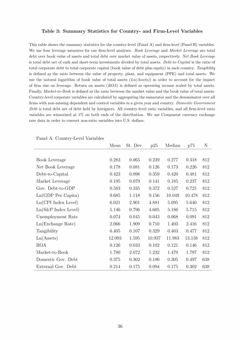
Table 3: Summary Statistics for Country- and Firm-Level Variables

This table shows the summary statistics for the country-level (Panel A) and firm-level (Panel B) variables.We use four leverage measures for our firm-level analyses. Book Leverage and Market Leverage are totaldebt over book value of assets and total debt over market value of assets, respectively. Net Book Leverageis total debt net of cash and short-term investments divided by total assets. Debt-to-Capital is the ratio oftotal corporate debt to total corporate capital (book value of debt plus equity) in each country. Tangibilityis defined as the ratio between the value of property, plant, and equipment (PPE) and total assets. Weuse the natural logarithm of book value of total assets (Ln(Assets)) in order to account for the impactof firm size on leverage. Return on assets (ROA) is defined as operating income scaled by total assets.Finally, Market-to-Book is defined as the ratio between the market value and the book value of total assets.Country-level corporate variables are calculated by aggregating the numerator and the denominator over allfirms with non-missing dependent and control variables in a given year and country. Domestic GovernmentDebt is total debt net of debt held by foreigners. All country-level ratio variables, and all firm-level ratiovariables are winsorized at 1% on both ends of the distribution. We use Compustat currency exchangerate data in order to convert non-ratio variables into U.S. dollars.

Panel A: Country-Level VariablesMean St. Dev. p25 Median p75 N

Book Leverage 0.283 0.065 0.239 0.277 0.318 812Net Book Leverage 0.178 0.081 0.126 0.173 0.226 812Debt-to-Capital 0.423 0.098 0.359 0.420 0.481 812Market Leverage 0.195 0.079 0.141 0.185 0.237 812Gov. Debt-to-GDP 0.583 0.335 0.372 0.527 0.725 812Ln(GDP Per Capita) 9.685 1.118 9.156 10.049 10.478 812Ln(CPI Index Level) 6.021 2.901 4.881 5.095 5.640 812Ln(S&P Index Level) 5.146 0.796 4.605 5.186 5.715 812Unemployment Rate 0.074 0.045 0.043 0.068 0.091 812Ln(Exchange Rate) 2.066 1.909 0.710 1.403 2.416 812Tangibility 0.405 0.107 0.329 0.403 0.477 812Ln(Assets) 12.093 1.595 10.937 11.983 13.138 812ROA 0.126 0.033 0.102 0.121 0.146 812Market-to-Book 1.780 2.072 1.232 1.470 1.797 812Domestic Gov. Debt 0.375 0.302 0.190 0.305 0.497 638External Gov. Debt 0.214 0.175 0.094 0.175 0.302 638

36

Summary Statistics for Country- and Firm-Level Variables (Cont.)

Panel B: Firm-Level VariablesMean St. Dev. p25 Median p75 N

Book Leverage 0.217 0.205 0.034 0.184 0.340 344132Net Book Leverage 0.050 0.324 -0.136 0.078 0.265 344117Debt-to-Capital 0.297 0.253 0.049 0.270 0.483 337205Market Leverage 0.181 0.179 0.019 0.132 0.290 330893Tangibility 0.305 0.232 0.113 0.261 0.447 344132Ln(Assets) 5.099 2.086 3.724 5.069 6.422 344132ROA 0.042 0.252 0.025 0.084 0.141 344132Market-to-Book 1.744 1.590 0.946 1.232 1.858 344132

37

Table 4: Leverage Regressions (Fixed Effects)

This table reports the coefficient estimates from the following fixed effects regression: Leveragej,t = β0

+ β1Government Debt-to-GDPj,t−1 + β2Corporate controlsj,t−1 + β3Macro controlsj,t−1 + uj + δt +εj,t, where j and t denote the country and year, respectively. Leverage denotes one of the following debtmeasures: Book Leverage is defined as the ratio of total book debt of all firms in a country to their totalassets; Net Book Leverage is total debt net of cash and short-term investments divided by total assets;Debt-to-Capital is the ratio of total corporate debt to total corporate capital (book value of debt plusequity) in each country; and Market Leverage is defined as the ratio of total book debt of all firms in acountry to their market value of assets. All other variables are explained in Table 2 and Table 3. Allregressions include country-fixed effects (uj) and year-fixed effects (δt). Standard errors are clustered atthe country level. Statistical significance at the 10%, 5% and 1% levels are denoted by “*”, “**” and “***”,respectively.

Panel A: All countries Panel B: OECD countries only

Book Net Book Debt-to Market Book Net Book Debt-to MarketLeverage Leverage Capital Leverage Leverage Leverage Capital Leverage

Gov. Debt-to-GDPt−1 -0.075*** -0.086*** -0.096*** -0.056** -0.080*** -0.096*** -0.099** -0.048*(-3.455) (-3.413) (-2.993) (-2.269) (-3.281) (-2.943) (-2.469) (-2.003)

Ln(GDP Per Capitat−1) 0.013 0.021 0.047* 0.028 -0.031 -0.045 0.017 0.019(0.585) (0.720) (1.874) (0.964) (-0.953) (-1.265) (0.451) (0.495)

Ln(CPI Index Levelt−1) 0.015 -0.020 0.028 -0.022 0.027 -0.014 0.059 -0.002(0.579) (-0.498) (0.813) (-0.558) (0.845) (-0.280) (0.998) (-0.049)

Ln(S&P Index Levelt−1) -0.016 -0.020 -0.032* -0.049*** -0.024 -0.038* -0.044* -0.049**(-1.354) (-1.254) (-2.020) (-3.660) (-1.348) (-1.748) (-1.969) (-2.449)

Unemployment Ratet−1 0.267*** 0.106 0.324** 0.133 0.134 -0.066 0.206 0.146*(2.919) (0.834) (2.423) (1.160) (1.139) (-0.420) (1.180) (1.886)

Ln(Exchange Ratet−1) -0.016*** -0.017*** -0.015* -0.014*** -0.013*** -0.012** -0.013 -0.009**(-3.377) (-3.555) (-1.864) (-3.345) (-3.045) (-2.647) (-1.647) (-2.660)

Tangibilityt−1 0.044 0.218** -0.065 0.135 0.026 0.170 -0.025 0.071(0.586) (2.084) (-0.624) (1.552) (0.301) (1.548) (-0.183) (0.950)

Ln(Assetst−1) -0.001 -0.004 0.007 -0.010 0.028** 0.047*** 0.030* 0.018(-0.141) (-0.325) (0.614) (-1.082) (2.341) (3.414) (1.885) (1.492)

ROAt−1 -0.820*** -0.897*** -1.179*** -1.062*** -0.849*** -0.777*** -1.318*** -0.858***(-5.492) (-4.577) (-5.619) (-4.237) (-4.732) (-4.145) (-5.034) (-3.888)

Market-to-Bookt−1 -0.000 -0.001 0.003* -0.007*** 0.007 0.012 0.015 -0.022(-0.062) (-0.588) (1.955) (-2.780) (1.042) (1.535) (1.421) (-1.695)

Observations 812 812 812 812 567 567 567 567Adj. R-squared 0.694 0.689 0.747 0.710 0.661 0.653 0.704 0.751Year FE YES YES YES YES YES YES YES YESCountry FE YES YES YES YES YES YES YES YES

38

Table 5: Leverage Regressions (First Differences)

This table estimates the following first difference specification: ∆Leveragej,t,t−1 = β0 + β1∆GovernmentDebt-to-GDPj,t−1,t−2 + β2∆Corporate controlsj,t−1,t−2 + β3∆Macro controlsj,t−1,t−2 + δt + εj,t, where jand t denote the country and year, respectively. Leverage denotes one of the following debt measures: BookLeverage is defined as the ratio of total book debt of all firms in a country to their total assets; Net BookLeverage is total debt net of cash and short-term investments divided by total assets; Debt-to-Capital isthe ratio of total corporate debt to total corporate capital (book value of debt plus equity) in each country;and Market Leverage is defined as the ratio of total book debt of all firms in a country to their marketvalue of assets. All other variables are explained in Table 2 and Table 3. All regressions include year-fixedeffects (δt). Standard errors are clustered at the country level. Statistical significance at the 10%, 5% and1% levels are denoted by “*”, “**” and “***”, respectively.

Panel A: All countries Panel B: OECD countries only

∆ Book ∆ Net Book ∆ Debt-to ∆ Market ∆ Book ∆ Net Book ∆ Debt-to ∆ MarketLeverage Leverage Capital Leverage Leverage Leverage Capital Leverage

∆ Gov. Debt-to-GDPt−1,t−2 -0.068*** -0.077*** -0.108*** -0.059* -0.064** -0.067** -0.083** -0.026(-3.194) (-3.511) (-3.586) (-1.836) (-2.669) (-2.644) (-2.446) (-0.927)

∆ Ln(GDP Per Capitat−1,t−2) 0.031** 0.040** 0.046** 0.041* 0.061*** 0.078*** 0.096*** 0.082***(2.180) (2.219) (2.261) (1.953) (3.915) (4.220) (4.272) (4.752)

∆ Ln(CPI Index Levelt−1,t−2) -0.034 -0.031 -0.048 -0.022 -0.066 -0.061 -0.083 -0.037(-1.027) (-0.692) (-0.835) (-0.356) (-1.524) (-0.925) (-0.973) (-0.529)

∆ Ln(S&P Index Levelt−1,t−2) -0.005 -0.006 -0.003 -0.011 -0.003 -0.006 -0.003 0.001(-0.880) (-1.000) (-0.453) (-1.353) (-0.372) (-0.671) (-0.318) (0.140)

∆ Unemployment Ratet−1,t−2 -0.109 -0.293** -0.083 -0.102 -0.052 -0.259* -0.063 -0.046(-1.267) (-2.362) (-0.664) (-0.757) (-0.645) (-2.044) (-0.465) (-0.427)

∆ Ln(Exchange Ratet−1,t−2) -0.001 0.001 -0.000 -0.003 -0.001 0.002 0.001 -0.002(-0.764) (0.402) (-0.081) (-1.068) (-0.351) (0.654) (0.325) (-0.775)

∆ Tangibilityt−1,t−2 0.005 0.039 -0.077 -0.029 0.054 0.029 0.011 -0.002(0.101) (0.554) (-0.992) (-0.458) (0.656) (0.251) (0.098) (-0.031)

∆ Ln(Assets)t−1,t−2 -0.000 0.003 0.005 0.013** 0.008 0.009 0.013 0.016**(-0.058) (0.339) (0.653) (2.184) (1.078) (0.723) (1.130) (2.225)

∆ ROAt−1,t−2 -0.148** -0.122 -0.187* -0.143 -0.230** -0.150 -0.273* -0.283**(-2.181) (-1.267) (-1.942) (-1.224) (-2.532) (-1.263) (-1.898) (-2.718)

∆ Martket-to-Bookt−1,t−2 -0.001** -0.001* -0.001*** -0.003** 0.001 0.000 0.001 -0.007**(-2.536) (-1.739) (-2.904) (-2.065) (0.396) (0.100) (0.349) (-2.452)

Observations 779 779 779 779 546 546 546 546Adj. R-squared 0.188 0.203 0.192 0.389 0.231 0.254 0.237 0.469Year FE YES YES YES YES YES YES YES YES

39

Table 6: External Debt (Country-Level)

This table investigates the impact of external government debt on corporate leverage by repeating both thefixed effects and the first difference specifications in Table 4 and Table 5 after decomposing GovernmentDebt-to-GDP as Domestic Government Debt and External Government Debt measured in percent of GDP.External Government Debt is government debt held by foreigners. Domestic Government Debt is Govern-ment Debt-to-GDP net of external debt. Standard errors are clustered at the country level. Statisticalsignificance at the 10%, 5% and 1% levels are denoted by “*”, “**” and “***”, respectively.

Fixed Effects First Difference

Book Net Book Debt-to Market ∆ Book ∆ Net Book ∆ Debt-to ∆ MarketLeverage Leverage Capital Leverage Leverage Leverage Capital Leverage

Domestic Gov. Debtt−1 -0.166*** -0.227*** -0.218*** -0.167*** -0.129*** -0.150*** -0.155*** -0.140***(-5.076) (-6.071) (-3.377) (-4.209) (-4.993) (-3.923) (-4.577) (-3.013)

External Gov. Debtt−1 0.028 0.004 0.003 0.043 -0.000 -0.002 -0.027 -0.003(0.705) (0.078) (0.058) (0.961) (-0.006) (-0.067) (-0.644) (-0.070)

Ln(GDP Per Capitat−1) 0.017 0.011 0.055*** 0.023 0.030** 0.032* 0.037** 0.033(1.174) (0.513) (2.716) (0.806) (2.239) (1.773) (2.226) (1.252)

Ln(CPI Index Levelt−1) 0.040 -0.012 0.035 -0.034 -0.016 -0.034 0.017 -0.044(1.259) (-0.250) (0.746) (-0.641) (-0.430) (-0.725) (0.341) (-0.535)

Ln(S&P Index Levelt−1) -0.006 -0.004 -0.025* -0.038*** -0.005 -0.007 -0.004 -0.014(-0.637) (-0.303) (-1.758) (-2.802) (-0.846) (-1.028) (-0.449) (-1.424)

Unemployment Ratet−1 0.289** 0.265 0.393** 0.107 -0.019 -0.142 -0.043 0.016(2.088) (1.434) (2.106) (0.630) (-0.201) (-1.281) (-0.352) (0.097)

Ln(Exchange Ratet−1) -0.005 -0.006 -0.001 -0.005** 0.000 0.004 0.001 -0.001(-1.411) (-1.487) (-0.139) (-2.067) (0.050) (0.977) (0.349) (-0.331)

Tangibilityt−1 0.089 0.274*** -0.022 0.180** -0.005 0.043 -0.070 0.009(1.331) (2.963) (-0.213) (2.043) (-0.093) (0.774) (-0.965) (0.112)

Ln(Assetst−1) -0.000 -0.002 0.009 -0.005 0.000 0.008 0.009 0.017*(-0.069) (-0.240) (1.084) (-0.953) (0.057) (0.799) (0.809) (1.971)

ROAt−1 -0.689*** -0.751*** -0.986*** -1.047*** -0.047 -0.040 -0.094 -0.069(-5.082) (-3.759) (-4.935) (-4.378) (-0.610) (-0.374) (-0.837) (-0.481)

Market-to-Bookt−1 0.001 -0.000 0.003** -0.006** -0.001 -0.001 -0.000 -0.004(1.475) (-0.543) (2.625) (-2.375) (-1.144) (-1.146) (-0.523) (-1.181)

Observations 633 633 633 633 592 592 592 592Adj. R-squared 0.752 0.765 0.785 0.751 0.195 0.234 0.197 0.418Year FE YES YES YES YES YES YES YES YESCountry FE YES YES YES YES NO NO NO NO

40

Table 7: Alternative Specification (Country-Level)

Corporate Debt is calculated by summing dollar value of debt over all firms in a country and year. NetCorporate Debt is the sum of total debt net of cash and short-term investments over all firms in a countryand year. Ln(Government Debt) is the natural logarithm of the dollar value of government debt outstand-ing. Standard errors are clustered at the country level. Statistical significance at the 10%, 5% and 1%levels are denoted by “*”, “**” and “***”, respectively.


Ln(Corp. Debt) Ln(Net Corp. Debt) ∆ Ln(Corp. Debt) ∆ Ln(Net Corp. Debt)

Ln(Gov. Debtt−1) -0.143** -0.370** -0.199*** -0.306**(-2.237) (-2.472) (-2.926) (-2.345)

Ln(GDP Per Capitat−1) 0.145 0.222 -0.043 0.324(1.626) (0.998) (-0.371) (1.462)

Ln(CPI Index Levelt−1) 0.111 0.125 0.236 -0.480(1.094) (0.472) (0.696) (-0.895)

Ln(S&P Index Levelt−1) 0.033 -0.032 0.160*** 0.195**(0.790) (-0.308) (3.768) (2.308)

Unemployment Ratet−1 1.109*** 1.298 -0.544 1.115(2.813) (1.417) (-0.652) (0.803)

Ln(Exchange Ratet−1) -0.045*** -0.066* 0.031 0.043(-2.708) (-1.741) (1.634) (1.377)

Tangibilityt−1 0.084 0.908* 0.182 -0.572(0.304) (1.720) (0.488) (-0.591)

Ln(Assetst−1) 1.006*** 1.135*** 0.897*** 1.124***(25.605) (5.849) (11.850) (2.756)

ROAt−1 -2.051*** -4.669*** 0.509 -1.094(-3.954) (-3.134) (1.218) (-0.775)

Market-to-Bookt−1 0.002 0.001 0.003 -0.001(0.887) (0.062) (0.447) (-0.232)

Observations 812 797 778 762Adj. R-squared 0.990 0.935 0.681 0.360Year FE YES YES YES YESCountry FE YES YES NO NO

41

Table 8: Country Characteristics and Crowding Out

This table reports the results from our first difference specification with change in government debt-to-GDP interacted with various country characteristics.Every year we split countries into terciles by their lagged Market Capitalization, Bank Dependence and Stock Turnover Ratio. Market Capitalization istotal market value of public firms as a percent of GDP. Bank Dependence is measured by total bank credit to private sector as a fraction of total credit.Stock Turnover Ratio is the value of domestic shares traded divided by their market capitalization. Standard errors are clustered at the country level.Statistical significance at the 10%, 5% and 1% levels are denoted by “*”, “**” and “***”, respectively.

Panel A Small Equity Market Medium Equity Market Large Equity Market

∆ Book ∆ Net Book ∆ Debt-to ∆ Market ∆ Book ∆ Net Book ∆ Debt-to ∆ Market ∆ Book ∆ Net Book ∆ Debt-to ∆ MarketLeverage Leverage Capital Leverage Leverage Leverage Capital Leverage Leverage Leverage Capital Leverage

∆ Gov. Debt-to-GDPt−1,t−2 -0.040 -0.040 -0.079* 0.008 -0.047 -0.039 -0.070 -0.048 -0.087** -0.111** -0.148** -0.100(-1.379) (-1.195) (-1.731) (0.186) (-1.025) (-0.826) (-1.114) (-0.999) (-2.611) (-2.599) (-2.597) (-1.605)

Observations 251 251 251 251 245 245 245 245 238 238 238 238Adj. R-squared 0.219 0.248 0.230 0.424 0.236 0.240 0.208 0.514 0.182 0.159 0.222 0.430Year FE YES YES YES YES YES YES YES YES YES YES YES YESControls YES YES YES YES YES YES YES YES YES YES YES YES

Panel B Low Bank Credit Medium Bank Credit High Bank Credit


∆ Gov. Debt-to-GDPt−1,t−2 -0.103*** -0.118*** -0.135*** -0.098*** -0.018 -0.011 -0.046 0.117* -0.047 -0.078 -0.066 -0.112(-4.733) (-5.165) (-4.143) (-4.036) (-0.334) (-0.190) (-0.668) (1.850) (-1.131) (-1.405) (-1.186) (-1.445)


40

Country Characteristics and Crowding Out

Panel C Low Stock Turnover Medium Stock Turnover High Stock Turnover


∆ Gov. Debt-to-GDPt−1,t−2 0.001 -0.017 -0.000 0.016 -0.083* -0.116** -0.107* -0.077 -0.104*** -0.112** -0.192*** -0.096*(0.028) (-0.502) (-0.012) (0.352) (-1.929) (-2.091) (-1.800) (-1.568) (-2.850) (-2.451) (-5.526) (-1.984)


41

Table 9: Firm-Level Analysis

This table reports the coefficient estimates from the following fixed effects regression: Leveragei,t = β0 +β1Government Debt-to-GDPj,t−1 + β2Macro controlsj,t−1 + β3Company controlsi,t−1 + ui + δt + εi,t, andthe following first difference regression: ∆Leveragei,t,t−1 = β0 + β1∆Government Debt-to-GDPj,t−1,t−2

+ β2∆Macro controlsj,t−1,t−2 + β3∆ Company controlsi,t−1,t−2 + δt + εi,t where i and j denote the firmand its country of incorporation, respectively. All regressions include firm fixed effects (ui) and year-fixedeffects (δt). Standard errors are clustered at the country level. Statistical significance at the 10%, 5% and1% levels are denoted by “*”, “**” and “***”, respectively.



Gov. Debt-to-GDPt−1 -0.069*** -0.053*** -0.077*** -0.048*** -0.099*** -0.098*** -0.099*** -0.073***(-5.110) (-3.053) (-4.200) (-3.143) (-3.500) (-3.701) (-4.117) (-3.826)

Ln(GDP Per Capitat−1) -0.027*** -0.025*** -0.025** -0.010 0.005 0.007 0.005 -0.001(-3.316) (-2.802) (-2.611) (-0.655) (0.409) (0.590) (0.532) (-0.038)

Ln(CPI Index Levelt−1) 0.009 0.016 0.034 0.016 -0.049 -0.062 -0.043 -0.032(0.378) (0.521) (1.010) (0.580) (-1.312) (-1.080) (-1.304) (-0.774)

Ln(S&P Index Levelt−1) -0.016** -0.028*** -0.018* -0.046*** -0.004 -0.004 -0.002 -0.008(-2.482) (-3.234) (-2.002) (-5.672) (-1.369) (-1.025) (-0.526) (-1.255)

Unemployment Ratet−1 0.032 -0.018 0.061 -0.102 0.007 0.032 -0.056 -0.223**(0.432) (-0.169) (0.562) (-0.957) (0.096) (0.327) (-0.606) (-2.432)

Ln(Exchange Ratet−1) -0.012*** -0.014*** -0.013** -0.014** -0.004*** -0.003 -0.005*** -0.003(-3.284) (-3.866) (-2.351) (-2.596) (-3.306) (-1.301) (-3.666) (-1.124)

Tangibilityt−1 0.126*** 0.358*** 0.147*** 0.106*** 0.043*** 0.002 0.055*** 0.038***(7.483) (14.120) (6.063) (6.101) (5.503) (0.170) (5.441) (5.077)

Ln(Assetst−1) 0.037*** 0.060*** 0.048*** 0.042*** 0.006*** 0.032*** 0.011*** 0.019***(8.001) (11.407) (7.585) (9.912) (3.506) (15.734) (7.263) (8.884)

ROAt−1 -0.106*** -0.105*** -0.103*** -0.076*** -0.031*** -0.046*** -0.017*** -0.014***(-7.914) (-6.830) (-5.493) (-5.345) (-5.063) (-7.831) (-6.412) (-7.998)

Market-to-Bookt−1 -0.004*** -0.009*** -0.005*** -0.011*** -0.001** -0.002** -0.002*** 0.001***(-3.602) (-6.518) (-2.804) (-12.137) (-2.595) (-2.595) (-4.534) (3.886)

Observations 344,132 344,117 337,205 330,893 299,540 299,524 294,217 288,621Adj. R-squared 0.639 0.717 0.707 0.726 0.0103 0.0128 0.0112 0.0637Year FE YES YES YES YES YES YES YES YESFirm FE YES YES YES YES NO NO NO NO

44

Table 10: Government Debt and Company Characteristics

Columns (1)-(3) and (4)-(6) report the results from firm fixed effects regression with firm size and prof-itability interactions. Size Tercile (ROA Tercile) indicates whether a firm’s lagged total assets (laggedROA) are in the second or third (highest) tercile of its country in a given year and zero otherwise. All re-gressions include firm and year-fixed effects. Standard errors are clustered at the country level. Statisticalsignificance at the 10%, 5% and 1% levels are denoted by “*”, “**” and “***”, respectively.

(1) (2) (3) (4) (5) (6) (7) (8)Book Net Book Debt-to Market Book Net Book Debt-to Market

Leverage Leverage Capital Leverage Leverage Leverage Capital Leverage

Gov. Debt-to-GDPt−1 -0.059*** -0.041** -0.064*** -0.044** -0.061*** -0.040** -0.070*** -0.042***(-4.051) (-2.160) (-3.316) (-2.667) (-4.585) (-2.226) (-3.984) (-2.763)

X Size Tercile 2 -0.009** -0.016* -0.012* -0.006(-2.378) (-2.005) (-1.995) (-0.904)

X Size Tercile 3 -0.016*** -0.018 -0.020** -0.009(-3.599) (-1.280) (-2.442) (-1.245)

X ROA Tercile 2 -0.013*** -0.020*** -0.015*** -0.013***(-3.990) (-2.857) (-5.249) (-4.867)

X ROA Tercile 3 -0.024*** -0.035*** -0.029*** -0.024***(-5.509) (-4.323) (-5.667) (-6.552)

Size Tercile 2 0.010** 0.020*** 0.008 0.011*(2.305) (4.113) (1.255) (1.724)

Size Tercile 3 0.028*** 0.040*** 0.028*** 0.029***(4.251) (3.112) (3.826) (3.524)

ROA Tercile 2 -0.001 0.006 -0.009* -0.001(-0.206) (0.598) (-1.876) (-0.236)

ROA Tercile 3 -0.013** -0.012 -0.029*** -0.025***(-2.247) (-1.037) (-4.149) (-5.051)

Ln(GDP Per Capitat−1) -0.028*** -0.027*** -0.026** -0.011 -0.027*** -0.025** -0.024*** -0.009(-3.215) (-2.859) (-2.621) (-0.742) (-3.014) (-2.592) (-2.752) (-0.543)

Ln(CPI Index Levelt−1) 0.009 0.016 0.034 0.017 0.007 0.015 0.032 0.016(0.370) (0.512) (1.014) (0.591) (0.324) (0.480) (0.948) (0.540)

Ln(S&P Index Levelt−1) -0.016** -0.027*** -0.018* -0.045*** -0.017** -0.029*** -0.020** -0.048***(-2.268) (-3.075) (-1.900) (-5.525) (-2.565) (-3.291) (-2.122) (-5.648)

Unemployment Ratet−1 0.050 0.011 0.073 -0.077 0.033 -0.014 0.060 -0.102(0.636) (0.098) (0.647) (-0.734) (0.437) (-0.125) (0.543) (-0.916)

Ln(Exchange Ratet−1) -0.012*** -0.014*** -0.013** -0.013** -0.012*** -0.015*** -0.013** -0.014**(-3.222) (-3.840) (-2.351) (-2.542) (-3.234) (-3.809) (-2.324) (-2.538)

Tangibilityt−1 0.126*** 0.357*** 0.147*** 0.105*** 0.127*** 0.358*** 0.148*** 0.107***(7.467) (14.114) (6.056) (6.099) (7.294) (13.962) (5.889) (6.012)

Ln(Assetst−1) 0.034*** 0.056*** 0.046*** 0.038*** 0.037*** 0.060*** 0.048*** 0.041***(6.574) (9.208) (6.890) (9.529) (7.880) (10.994) (7.438) (9.770)

ROAt−1 -0.105*** -0.104*** -0.102*** -0.075*** -0.086*** -0.083*** -0.066*** -0.046***(-7.763) (-6.767) (-5.344) (-5.244) (-9.939) (-9.648) (-5.435) (-5.220)

Market-to-Bookt−1 -0.004*** -0.009*** -0.005*** -0.011*** -0.002** -0.008*** -0.003* -0.009***(-3.580) (-6.375) (-2.795) (-12.586) (-2.342) (-5.136) (-1.819) (-11.299)

Observations 344,132 344,117 337,205 330,893 344,132 344,117 337,205 330,893Adj. R-squared 0.639 0.717 0.707 0.727 0.641 0.718 0.710 0.731Year FE YES YES YES YES YES YES YES YESFirm FE YES YES YES YES YES YES YES YES

45

Table 11: EMU Integration

Panel A investigates the impact of EMU integration on the sensitivity of corporate leverage to governmentdebt for the EMU countries. Panel B reports the results for all countries. EMU is a dummy variablethat indicates whether the country is a member of the European Monetary Union. All regressions areestimated for the first difference specification. All regressions include macro and firm controls used in thebaseline specification (Table 5). Sample period is from 1990 to 2006. Standard errors are clustered at thecountry level. Statistical significance at the 10%, 5% and 1% levels are denoted by “*”, “**” and “***”,respectively.

∆ Book ∆ Net Book ∆ Debt-to ∆ Market ∆ Book ∆ Net Book ∆ Debt-to ∆ MarketPanel A: EMU countries Leverage Leverage Capital Leverage Leverage Leverage Capital Leverage

∆ Gov. Debt-to-GDPt−1,t−2 -0.164** -0.160 -0.259** -0.106 -0.091* -0.078 -0.148** -0.030(-2.541) (-1.658) (-2.509) (-1.417) (-1.937) (-1.015) (-2.372) (-0.403)

X After 1999 0.322** 0.360* 0.394** 0.262** 0.261* 0.290 0.317* 0.159(3.020) (1.986) (2.733) (2.904) (2.134) (1.671) (2.010) (1.475)

After 1999 0.005 -0.000 0.004 0.014*(1.122) (-0.002) (0.569) (2.148)

Observations 162 162 162 162 162 162 162 162Adj. R-squared 0.130 0.0713 0.151 0.226 0.191 0.202 0.170 0.430Year FE NO NO NO NO YES YES YES YES

Panel B: All countries ∆ Book Leverage ∆ Net Book Leverage ∆ Debt-to-Capital ∆ Market Leverage

∆ Gov. Debt-to-GDPt−1,t−2 -0.154*** -0.110*** -0.147*** -0.111** -0.290*** -0.245*** -0.249*** -0.209**(-3.982) (-3.250) (-3.412) (-2.295) (-4.482) (-3.671) (-3.017) (-2.642)

X After 1999 X EMU 0.222** 0.215** 0.289* 0.251* 0.144 0.147 0.110 -0.023(2.049) (2.158) (1.706) (1.846) (0.884) (1.000) (0.804) (-0.216)

X After 1999 0.042 0.026 0.023 0.029 0.170 0.162 0.103 0.135(0.715) (0.469) (0.316) (0.403) (1.663) (1.638) (0.953) (1.389)

X EMU 0.008 0.028 0.019 0.057 0.074 0.091 0.186* 0.197**(0.133) (0.461) (0.222) (0.656) (0.691) (0.941) (1.996) (2.453)

After 1999 X EMU 0.011** 0.011** 0.014** 0.015** 0.014** 0.015** 0.026*** 0.028***(2.211) (2.255) (2.568) (2.676) (2.043) (2.150) (3.124) (3.276)

After 1999 -0.008*** -0.013*** -0.011** -0.015**(-2.939) (-4.217) (-2.601) (-2.684)

EMU 0.002 0.002 0.002 0.002 0.001 0.001 -0.012* -0.011*(0.447) (0.613) (0.398) (0.455) (0.119) (0.201) (-1.843) (-1.739)

Observations 464 464 464 464 464 464 464 464Adj. R-squared 0.110 0.210 0.0952 0.191 0.108 0.175 0.108 0.291Year FE NO YES NO YES NO YES NO YES

46

Table 12: EMU Integration and Firm Characteristics

This table investigates the impact of EMU integration on the sensitivity of corporate leverage to governmentdebt for companies with different sizes and levels of profitability. The sample period is between 1990 and2006 and is restricted to companies incorporated in an EMU member country. After 1999 is one (zero)for the years between 1999 and 2006 (1990 and 1998). All regressions are estimated for the first differencespecification. Standard errors are clustered at the country level. Statistical significance at the 10%, 5%and 1% levels are denoted by “*”, “**” and “***”, respectively.

∆ Book Leverage

Size (Book Assets) Profitability

Low Medium High Low Medium High

After 1999 0.003 0.004 0.001 0.006** 0.004 -0.003(0.912) (1.710) (0.368) (2.321) (1.776) (-1.000)

∆ Gov. Debt-to-GDPt−1,t−2 -0.070 -0.092 -0.098** -0.086 -0.069 -0.120**(-1.333) (-1.655) (-2.515) (-1.756) (-1.158) (-2.931)

X After 1999 0.045 0.070 0.138* 0.044 0.045 0.171**(0.477) (0.593) (2.089) (0.437) (0.760) (2.256)

∆ Ln(GDP Per Capitat−1,t−2) -0.037* -0.042** -0.034*** -0.021 -0.032* -0.068***(-1.870) (-3.062) (-3.629) (-1.577) (-2.039) (-5.542)

∆ Ln(CPI Index Levelt−1,t−2) -0.019 -0.023 -0.010 -0.088 0.005 0.050(-0.131) (-0.116) (-0.104) (-0.606) (0.039) (0.353)

∆ Ln(S&P Index Levelt−1,t−2) -0.016*** -0.007 -0.003 -0.023*** -0.005 0.003(-3.564) (-1.585) (-0.611) (-4.388) (-0.760) (1.520)

∆ Unemployment Ratet−1,t−2 -0.422* -0.114 -0.683*** -0.220* -0.345** -0.667***(-2.154) (-0.919) (-4.107) (-1.911) (-2.551) (-8.089)

∆ Ln(Exchange Ratet−1,t−2) -0.005* -0.004** -0.000 -0.002 -0.002* -0.003*(-2.085) (-2.810) (-0.112) (-1.602) (-1.841) (-1.851)

∆ Tangibilityt−1,t−2 0.011 0.047 0.078*** 0.040 0.073*** 0.018(0.362) (1.437) (4.685) (1.446) (3.630) (0.385)

∆ Ln(Assets)t−1,t−2 0.010 0.019*** 0.004 0.003 0.016** 0.027***(1.107) (4.300) (0.603) (0.241) (2.439) (5.617)

∆ ROAt−1,t−2 -0.025** -0.011 -0.052** -0.012 -0.067*** -0.012(-2.492) (-0.529) (-2.657) (-0.780) (-4.095) (-0.945)

∆ Martket-to-Bookt−1,t−2 0.003 -0.001 0.000 0.002 -0.002 0.001(1.503) (-0.831) (0.108) (0.790) (-0.748) (0.523)

Observations 4,905 5,571 5,986 5,373 5,625 5,464Adj. R-squared 0.008 0.010 0.013 0.007 0.015 0.016

47

Appendix

A.1 Proof of Implication 1

In order to investigate the impact of government debt on the equilibrium leverage

ratio, we first substitute equation (6) into (5) to obtain

θ(d∗ − λ) = ρv′(ρd∗(1− wG) + wG). (14)

Then, we take the derivative of both sides in equation (14) with respect to wG, and solve

for ∂d∗/∂wG.

[θ − ρ2(1− wG)v′′(ρd∗(1− wG) + wG)

] ∂d∗∂wG

= ρ (1− ρd∗) v′′(ρd∗(1− wG) + wG). (15)

Given that v′′(.) < 0, ρ ≤ 1, and d∗ < 1, equation (15) implies that

∂d∗

∂wG< 0.

Similarly, taking the partial derivative of both sides in equation (6) yields

∂w∗D∂wG

= ∂d∗

∂wG(1− wG)− d∗,

which implies that∂w∗D∂wG

< 0.

Thus, as government debt increases, both d∗ and w∗D decrease relative to the previous

equilibrium. When government debt increases, households absorb the increase by in-

creasing their allocation wG. We will prove by contradiction that both d∗ and w∗D should

decrease. Assume counterfactually that d∗ increases. Then the second equality in (5)

implies that v′ increases. Since v′′ < 0, v′′ increases only if ρw∗D + wG decreases. Given

the increase in wG, ρw∗D has to decrease more than the increase in wG. Note that in equi-

librium, ρw∗D = ρd∗(1 − wG) which implies that every percent increase in wG decreases

ρw∗D by less than one percent. Thus, an increase in d∗ is not feasible. The only feasible

equilibrium response is for both d∗ and w∗D to decrease when government debt increases.

48


First, solve for d∗ and d∗∗ using equation (4), respectively

EP ∗i = θ (d∗i − λ) and EP ∗∗i = θ(d∗∗i − λ).

Taking the differences between the equity premiums yields

EP ∗i − EP ∗∗i = θi(d∗i − d∗∗i ).

Finally, by solving for θi we obtain

θi = EP ∗i − EP ∗∗id∗i − d∗∗i

.

which implies

θH = EP ∗H − EP ∗∗Hd∗H − d∗∗H

>EP ∗L − EP ∗∗Ld∗L − d∗∗L

= θL. (16)


Equation (11) implies that

v′ (ρLwDL+ ρHwDH

+ wG) = θ(d∗L − λ)

ρL= θ

(d∗H − t)ρH

. (17)

We obtain the following expression by taking the derivative of both sides with respect to

share of government debt (wG)

1ρL

∂d∗L∂wG

= 1ρH

∂d∗H∂wG

. (18)

Given that ρH > ρL, it follows from equation (18) that the absolute value of the derivative

of the leverage ratio with respect to government debt for the high-theta firm exceeds that

for the low-theta firm such that ∣∣∣∣∣∂d∗H∂wG

∣∣∣∣∣ >∣∣∣∣∣ ∂d∗L∂wG

∣∣∣∣∣

49

A.4 Proof of Implication 3 for θ

We also analyze the model’s implications for two firms that are incorporated in the

same country but are subject to different levels of financing frictions proxied by θ assuming

that their debt securities contribute to the household’s marginal utility by the same

amount (ρL = ρH = ρ). It follows from equation (9) that in equilibrium rEH− rDH

=

rEL− rDL

. By combining equations (9) and (10) we obtain the following equilibrium

condition

r∗E − r∗D = ρv′(ρw∗DL+ ρw∗DH

+ wG) = θL (d∗L − λ) = θH (d∗H − λ) (19)

Debt and equity markets clear in equilibrium, and the household’s budget constraint is

satisfied

Ki = Ei +Di and W = EL + EH +DL +DH +G.

In order to understand the impact of government debt on leverage ratios, we take the

derivative of both sides of equation (19) with respect to the government ratio wG:

ρv′′(ρw∗DL+ ρw∗DH

+ wG)(

1 + ρ∂w∗L∂wG

+ ρ∂w∗H∂wG

)= θL

∂d∗L∂wG

= θH∂d∗H∂wG

. (20)

Given that θH > θL, equation (20) suggests that the absolute value of the marginal change

in the leverage ratio of the high-θ firm is less than that of the low-θ firm such that

∣∣∣∣∣∂d∗H∂wG

∣∣∣∣∣ <∣∣∣∣∣ ∂d∗L∂wG

∣∣∣∣∣ .Implication 3 (for θ): Within a country, for a given level of government debt increase,

firms that are subject to more financing frictions choose a smaller reduction in leverage

than firms with lower adjustment costs.

50

Table A1: Variable Definitions

This table details the variable construction for the analysis of the sample. Panel A lists the definitions ofCompustat variables. The variable Xpressfeed pneumonics are given in italic. The country-level variablesfollow firm-level definitions and are calculated by aggregating the numerator and denominator values overall firms in a given year and country. Panel B lists the data source for and the definitions of macro variables.If a variable is available through two different sources for a country, we use the data source that providesus with the longest series.

Panel A: Compustat Variables

Variable Compustat Item Name

Ln(Assets) Ln(Total Book Assets)ROA Income / Assets = oibdp / atTangibility Net PPE / Assets = ppent / atMarket-to-Book MVA / Total Book AssetsMarket Value of Assets = at - ceq + prcc × cshocTotal Debt Short-Term Debt + Long-Term Debt = dltt + dlcBook Leverage Total Debt / Total Book Assets = (dltt + dlc) / atDebt-to-Capital Total Debt / Total Capital = (dltt+dlc) / (ceq+dltt+dlc)Market Leverage Total Debt / Market Value of Assets

Panel B: Macro Variables

Variable Data Source Definition

Gov. Debt-to-GDP WEO data on IMF Gross government debt (%GDP)GDP Per Capita World Bank GDP per capita (current US$)Inflation World Bank and IMF Inflation, consumer prices (annual %)S&P Return World Bank S&P global equity indices (annual % change)Unemployment Rate World Bank and IMF Unemployment, total (% of total labor force)Nominal Exchange Rate World Bank and ECB Official exchange rate (LCU per US$, period avr.)External Government Debt IMF, World Bank and ECB Gross external debt (%GDP)Bank credit to private sector BIS Bank credit (% GDP)Stock Turnover Ratio World Bank Value of shares traded (% market capitalization)

51

Table A2: Alternative Specification (Firm-Level)

Corporate Debt is the sum of dollar value of long-term debt and debt in current liabilities. Ln(GovernmentDebt) is the natural logarithm of the dollar value of government debt outstanding. Standard errors areclustered at the country level. Statistical significance at the 10%, 5% and 1% levels are denoted by “*”,“**” and “***”, respectively.

Ln(Corporate Debt)


Ln(Gov. Debtt−1) -0.258*** -0.251***(-3.056) (-3.939)

Ln(GDP Per Capitat−1) 0.080 0.320***(0.678) (2.869)

Ln(CPI Index Levelt−1) 0.442 0.423(1.564) (0.863)

Ln(S&P Index Levelt−1) 0.067 0.108***(1.598) (3.284)

Unemployment Ratet−1 0.018 -1.272**(0.025) (-2.293)

Ln(Exchange Ratet−1) -0.092*** -0.027***(-3.308) (-4.223)

Tangibilityt−1 0.732*** 0.342***(4.933) (5.913)

Ln(Assetst−1) 0.788*** 0.167***(17.442) (15.303)

ROAt−1 -0.621*** -0.069***(-9.686) (-6.688)

Market-to-Bookt−1 0.011 0.015***(1.095) (7.349)

Observations 339,532 295,281Adj. R-squared 0.880 0.0161Year FE YES YESFirm FE YES NO

52

Table A3: External Debt (Firm-Level)

This table investigates the impact of external government debt on corporate leverage by repeating both thefixed effects and the first difference specifications in Table 9 after decomposing Government Debt-to-GDPas Domestic Government Debt and External Government Debt measured in percent of GDP. ExternalGovernment Debt is government debt held by foreigners. Domestic Government Debt is Government Debt-to-GDP net of external debt. Standard errors are clustered at the country level. Statistical significance atthe 10%, 5% and 1% levels are denoted by “*”, “**” and “***”, respectively.



Domestic Gov. Debtt−1 -0.039** -0.095** -0.038 -0.051** -0.071*** -0.096*** -0.087*** -0.042***(-2.047) (-2.599) (-1.382) (-2.061) (-2.777) (-2.839) (-3.682) (-2.817)

External Gov. Debtt−1 0.028 0.011 0.013 0.057 -0.012 -0.026 -0.035 -0.022(0.688) (0.215) (0.250) (1.285) (-0.338) (-0.642) (-0.980) (-0.471)

Ln(GDP Per Capitat−1) -0.031*** -0.047*** -0.028** -0.026** 0.006 0.003 0.004 -0.007(-3.813) (-3.959) (-2.187) (-2.378) (0.347) (0.188) (0.344) (-0.253)

Ln(CPI Index Levelt−1) 0.036 0.025 0.055 0.035 -0.018 -0.031 -0.013 0.035(1.443) (0.553) (1.514) (1.293) (-0.330) (-0.318) (-0.269) (0.877)

Ln(S&P Index Levelt−1) -0.015*** -0.023*** -0.018** -0.035*** -0.008*** -0.012** -0.006 -0.001(-3.179) (-2.912) (-2.485) (-5.697) (-2.887) (-2.120) (-1.564) (-0.081)

Unemployment Ratet−1 0.020 0.158 0.081 -0.175 0.046 0.074 0.004 -0.166(0.261) (1.150) (0.744) (-1.234) (0.441) (0.551) (0.037) (-1.338)

Ln(Exchange Ratet−1) -0.008** -0.007* -0.010** -0.009** -0.002** -0.002 -0.003** -0.002(-2.671) (-1.980) (-2.086) (-2.217) (-2.259) (-0.675) (-2.589) (-0.720)

Tangibilityt−1 0.122*** 0.334*** 0.141*** 0.096*** 0.041*** 0.002 0.050*** 0.033***(6.909) (21.003) (5.780) (5.264) (5.462) (0.100) (4.835) (6.076)

Ln(Assetst−1) 0.037*** 0.065*** 0.049*** 0.043*** 0.004** 0.031*** 0.010*** 0.017***(6.576) (13.426) (6.405) (7.503) (2.103) (9.933) (5.563) (5.704)

ROAt−1 -0.098*** -0.107*** -0.099*** -0.074*** -0.029*** -0.046*** -0.016*** -0.014***(-5.871) (-5.034) (-4.312) (-4.598) (-5.214) (-7.812) (-4.968) (-5.620)

Market-to-Bookt−1 -0.002** -0.007*** -0.002* -0.008*** -0.001 -0.001 -0.001*** 0.001(-2.388) (-6.715) (-2.006) (-7.796) (-1.418) (-1.406) (-5.366) (1.517)

Observations 231,440 231,434 227,453 222,072 196,245 196,237 193,219 188,358Adj. R-squared 0.679 0.751 0.744 0.759 0.00929 0.0124 0.0112 0.0760Year FE YES YES YES YES YES YES YES YESCountry FE YES YES YES YES NO NO NO NO

53

Table A4: Debt Maturity

This table reports the results from fixed effects and first difference regression of Long-Term Debt and Short-Term Debt as well as their ratio. Long-Term Debt is total debt due in more than one year. Short-TermDebt is debt in current liabilities. Standard errors are clustered at the country level. Statistical significanceat the 10%, 5% and 1% levels are denoted by “*”, “**” and “***”, respectively.

Fixed Effects First Differences

LT Debt/ ST Debt/ LT Debt/ ∆ LT Debt/ ∆ ST Debt/ ∆ LT Debt/Assets Assets ST Debt Assets Assets ST Debt

Gov. Debt-to-GDPt−1 -0.032** -0.036*** -0.029 -0.044*** -0.051*** -0.000(-2.082) (-3.810) (-0.644) (-3.574) (-2.942) (-0.002)

Ln(GDP Per Capitat−1) -0.017 -0.010 -0.023 -0.004 0.008 -0.013(-1.267) (-0.633) (-0.556) (-1.187) (0.828) (-0.528)

Ln(CPI Index Levelt−1) -0.031 0.039 -0.130 -0.044 -0.007 -0.074(-0.743) (1.301) (-1.008) (-1.471) (-0.291) (-0.974)

Ln(S&P Index Levelt−1) -0.001 -0.015*** 0.016 0.001 -0.005* -0.000(-0.240) (-4.322) (1.221) (0.327) (-1.930) (-0.056)

Unemployment Ratet−1 -0.012 0.042 0.083 -0.081 0.074 -0.045(-0.151) (0.591) (0.341) (-1.420) (1.198) (-0.249)

Ln(Exchange Ratet−1) -0.009*** -0.003* -0.012** -0.004*** -0.001 -0.005**(-3.332) (-2.014) (-2.576) (-3.423) (-0.706) (-2.033)

Tangibilityt−1 0.078*** 0.046*** 0.067*** 0.014** 0.029*** -0.029***(5.064) (11.883) (3.836) (2.296) (9.091) (-3.096)

Ln(Assetst−1) 0.027*** 0.010** 0.037*** 0.005*** 0.002 0.007***(14.740) (2.575) (22.888) (5.181) (1.523) (2.903)

ROAt−1 -0.045*** -0.051*** 0.020* -0.012*** -0.014*** -0.006(-8.079) (-6.043) (1.875) (-7.017) (-3.928) (-0.972)

Market-to-Bookt−1 -0.001 -0.002*** 0.004*** -0.000* -0.001*** 0.001(-1.157) (-6.773) (3.819) (-1.800) (-2.789) (0.999)

Observations 344,132 344,132 295,988 299,561 299,643 250,352Adj. R-squared 0.628 0.555 0.541 0.00368 0.00528 0.00117Year FE YES YES YES YES YES YESFirm FE YES YES YES NO NO NO

54

Government Debt and Capital Structure Decisions ...

Documents

Transcript of Government Debt and Capital Structure Decisions ...