Governing the Commons? - World...
55
Policy Research Working Paper 8351 Governing the Commons? Water and Power in Pakistan’s Indus Basin Hanan G. Jacoby Ghazala Mansuri Development Research Group Poverty and Inequality Team February 2018 WPS8351 Public Disclosure Authorized Public Disclosure Authorized Public Disclosure Authorized Public Disclosure Authorized
Transcript of Governing the Commons? - World...

Policy Research Working Paper 8351
Governing the Commons?
Water and Power in Pakistan’s Indus Basin
Hanan G. JacobyGhazala Mansuri
Development Research GroupPoverty and Inequality TeamFebruary 2018
WPS8351P
ublic
Dis
clos
ure
Aut
horiz
edP
ublic
Dis
clos
ure
Aut
horiz
edP
ublic
Dis
clos
ure
Aut
horiz
edP
ublic
Dis
clos
ure
Aut
horiz
ed

Produced by the Research Support Team
Abstract
The Policy Research Working Paper Series disseminates the findings of work in progress to encourage the exchange of ideas about development issues. An objective of the series is to get the findings out quickly, even if the presentations are less than fully polished. The papers carry the names of the authors and should be cited accordingly. The findings, interpretations, and conclusions expressed in this paper are entirely those of the authors. They do not necessarily represent the views of the International Bank for Reconstruction and Development/World Bank and its affiliated organizations, or those of the Executive Directors of the World Bank or the governments they represent.
Policy Research Working Paper 8351
This paper is a product of the Poverty and Inequality Team, Development Research Group. It is part of a larger effort by the World Bank to provide open access to its research and make a contribution to development policy discussions around the world. Policy Research Working Papers are also posted on the Web at http://econ.worldbank.org. The authors may be contacted at [email protected].
Surface irrigation is a common pool resource characterized by asymmetric appropriation opportunities across upstream and downstream water users. Large canal systems are also predominantly managed by the state. This paper studies water allocation under an irrigation bureaucracy subject to corruption and rent-seeking. Data on the landholdings and
political influence of nearly a quarter million irrigators in Pakistan’s vast Indus Basin watershed allow the construction of a novel index of lobbying power. Consistent with a model of misgovernance, the decline in water availability and land values from channel head to tail is accentuated along canals having greater lobbying power at the head than at the tail.

Governing the Commons?
Water and Power in Pakistan’s Indus Basin
Hanan G. Jacoby∗ Ghazala Mansuri†
Keywords: Bureaucracy, rent-seeking, corruption, common property resource, irrigation
JEL codes: D73, P48, Q15, Q25
∗World Bank ([email protected]), 1818 H St NW, Washington DC 20433. Funding for this projectwas provided by the World Bank’s Knowledge for Change Program, its Strategic Research Program, andits Research Support Budget. The project would not have been possible without the support of the PunjabIrrigation Department. The authors are particularly grateful to Mr. Habibullah Bodla at the PMIU forproviding access to the discharge data and to Mr. Afzal Toor at PIDA for facilitating the irrigation outletsurvey. The team also thanks Mr. Saif Anjum (ex-Secretary Irrigation) for his consistent support. The viewsexpressed herein are those of the authors, and do not necessarily reflect the opinions of the World Bank, itsexecutive directors, or the countries they represent.†World Bank ([email protected]).

1 Introduction
Human efforts to control the flow of water for agriculture gave rise to the world’s first great
civilizations,1 and today surface irrigation delivers lifeblood to tens of millions of farm-
ers across the globe. Gravity-flow surface irrigation is also significant as a common pool
resource. Because it is prohibitively costly to fully enforce off-take from a river or canal,
irrigation water is subject to appropriation by upstream users (“headenders”) at the expense
of those downstream (“tailenders”), a version of the tragedy of the commons.2 In Governing
the Commons, Ostrom (1990) argued that non-state institutions often arise organically to
avert such tragedies through collective action. Yet, private (free market) allocation of canal
water in large-scale irrigation systems faces daunting economic and technical hurdles (Sam-
path 1992). Instead, extensive irrigation bureaucracies have been established to operate
centralized systems for the allocation of water as it makes its way down from the rivers and
main canals to the network of distributaries, minor and sub-minor canals, and, finally, to
the watercourse outlets, where it is delivered to individual farms. While the dysfunction of
state-managed irrigation has been well documented (e.g., Wade 1982 and Chambers 1988),3
we lack a falsifiable theory of commons regulation that accounts for the differing incentives
within the bureaucratic hierarchy as well as between the regulator and the regulated.
In this paper we consider the interplay between bureaucratic management and common
property users, or rather groups of users, in the context of the world’s largest canal irriga-
tion system, that of the Indus Basin watershed of Pakistan. On this vast system, de jure
water allocations are based on a proportionality principle inherited from the British colonial
1Wittfogel (1957) famously claimed that the need to mobilize labor for large irrigation works and tomanage water allocation brought into being the authoritarian state.
2Bromley et al. (1980), Ostrom and Gardner (1993) and Ray and Williams (2002), among many others,highlight this locational asymmetry inherent in canal irrigation systems.
3Disappointment with the performance of state-run systems has sown the seeds for irrigation managementreform underway worldwide (Garces-Restrepo et al. 2007). In a companion paper (Jacoby et al. 2018), westudy just such a reform carried out in Pakistan’s Punjab province.
1

administration: to each according to his cultivable area. De facto allocations, however, are
determined by interactions between groups of farmers, organized by channel outlet, and the
provincial irrigation department. As we will argue, this interaction is characterized by both
corruption and rent-seeking. Corruption is of the “with theft” variety (Shleifer and Vishny,
1993), in that the farmers who pay the bribe and the local irrigation official who demands
it both benefit; the losers are the farmers at the downstream outlets who receive less water
than they are entitled to. Rent-seeking arises as coalitions of headenders and tailenders
lobby the higher irrigation department office to intercede on their behalf, e.g., by replacing
(or not replacing) the local official. In choosing how hard to lobby, we assume that the head
coalition takes into account the bribes its members must pay, while the rational local official
internalizes the rent-seeking induced by his own corruption.
Our theoretical model allows a role for political influence in the rent-seeking contest. Of
critical importance for the contest outcome is the distribution of lobbying power (or efficacy)
along a channel. We establish that, insofar as such influence is relatively greater at the head
reaches than at the tail, “theft” will be greater, which is to say that more water will be
diverted toward the head and away from the tail. Our model also has implications for the
value of farmland, which is assumed to reflect not only the productive value of the canal
water delivered but also the bribes that farmers may have to pay to ensure these deliveries.
Even though the bribe amount is increasing in the relative influence of headend landowners,
thus depressing their land values, we show that the productive value of the greater off-take at
the head more than makes up for this; thus, on balance, the head-tail land value differential
increases with relative head influence. Finally, the assumption of competitive rent-seeking
delivers a distinctive symmetry result: a one unit increase in lobbying influence of the head
coalition has an equivalent impact on the head-tail differential in both water availability and
land values as a one unit decrease in political influence of the tail coalition.
To test these implications, we have collected a truly unique data set on both landown-
2

ership and influential positions held by every water-user in each of 3,923 watercourses (out-
lets) along 448 channels throughout Punjab province; in all, we have information on about
220,000 individual farmers. Knowledge of these two dimensions of influence, land and official
position-holding, allows us to extend recent work equating political power with landowner-
ship (e.g., Anderson et al. 2015 and Baland and Robinson 2008). We construct a novel and
intuitively appealing index of lobbying power that takes into account the interaction between
irrigated lanholdings, a measure of an individual’s economic stake, and personal influence
aggregated across all members of each contending coalition. Landowners contribute to the
index more than in proportion to their economic stake insofar as they hold an influential
position (such as a local political office). Our empirical strategy exploits variation in canal
discharge and land values across head and tail outlets along the same channel, thus purging
channel-level unobservables that may be correlated with both lobbying influence and water
availability.
The main contribution of this paper is to develop and empirically test a political-economy
model of common pool resource management in the spirit of Krueger (1974). Past literature,
by contrast, is largely prescriptive, focusing on the welfare costs of overexploitation and the
optimal regulation of the resource by a benevolent social planner (e.g., Huang and Smith
2014 for the case of a fishery; Gisser 1983 and Timmins 2002 for the case of a groundwater
aquifer).4 We also contribute to a growing empirical literature concerned with bureaucratic
incentives and corruption (Reinikka and Svensson 2004; Olken 2007; Olken and Barron 2009;
Burgess et al. 2012; Neihaus and Sukhtanakar 2013). What differentiates our work is the
focus on competitive rent-seeking among the agents affected by the bureaucrat’s actions; in
other words, we recognize the political context in which a bureaucracy operates.5
4An important exception is Johnson and Libecap (1982), who consider the conflicting interests of hetero-geneous fisherman in the formation of fishery regulation along the Texas coast. In their context, however,corruption within the regulatory enforcement agency does not appear to be an issue.
5Reinikka and Svensson (2004) touch upon this issue by considering how communities interact withtheir local officials’ school-fund disbursement decision. Importantly, however, there is no inter-community
3

The remainder of the paper is organized as follows. In the next section, we provide
institutional background on the canal irrigation system in Pakistan, the basis upon which
we build our theoretical arguments in section 3. Section 4 describes the data collection effort
on the two aspects of political influence and on land values, as well as the measurement of
canal discharge in the Indus Basin. In Section 5, we present empirical tests of the theory,
consider alternative explanations for the results, and analyze their implications for wealth
inequality. We conclude in Section 6.
2 Indus Basin irrigation system
The Indus Basin irrigation system, which accounts for 80% of Pakistan’s agricultural pro-
duction, lies mostly in its most populous province, Punjab, wherein it encompasses 37,000
kilometers of canals and irrigates about 8.5 million hectacres. From the Indus, Jhelum,
Chenab, Ravi, and Sutlej Rivers, a dense network of main canals, branch canals, distribu-
taries, minors, and sub-minors ramify out, ultimately feeding 58,000 individual watercourses
in Punjab alone (See Figure 1 for a schematic of the canal hierarchy.).6
Each watercourse outlet or mogha supplies irrigation to typically several dozen farmers
according to a rotational system known as warabandi. The institution of warabandi (literally
“fixed turns”), which traces its origins to British colonial rule and to the early development
of irrigation in the Indus Basin, embodies a modified principle of equity: to each irrigator
in proportion to his cultivated area. At each level of the canal hierarchy in this continuous
gravity-flow irrigation system, “authorized discharge” is allocated in proportion to cultivable
command area (CCA). At the main canal level, irrigation department staff operate a series
competition for resources in their context and, hence, officials are not balancing opposing interests. Alsorelated, Banerjee et al. (2001) explore the implications of rent-seeking within private sugar cooperatives inIndia, focusing on the conflict of interest between large and small growers.
6On about a third of Punjab’s irrigation system, canal management was devolved, in fits and starts,to locally elected farmers organizations beginning in the early 2000s (see Jacoby et al. 2018). This paperfocuses on the remaining two-thirds of the system.
4

Head outlets Tail outlets
Dis
trib
uta
ry
Minor canal
Outlet discharge
Distance from head0
= PMIU discharge gauge
Branch canal Authorized
ActualDe-silted
Watercourse
Head
Tail
Figure 1: Channel schematic with discharge gauges
of gates regulating flow into the off-taking distributaries according to a rotational sched-
ule. However, since moghas are ungated, discharge into tertiary units, the watercourses, is
determined by the width of the outlet; the greater the watercourse CCA, the greater the
authorized outlet width and thus the greater the water in-take each week. Over the course
of a week, proceeding from the head to the tail of the watercourse, each farmer takes his pre-
assigned turn at using the entire flow to irrigate his field, with the length of turn proportional
to the size of the field.
Although design discharge at any point along a channel accounts for seepage and con-
veyance losses and is therefore a declining function of distance to the head (see Figure 1 inset),
tail outlets should, by virtue of their greater width, receive their full water entitlement.7 In
practice, however, this elaborately constructed allocation system does not guarantee equity.
If discharge at the distributary head is intermittent during the filling cycle (as is often the
7Since there is no adjustment for seepage within a watercourse, farmers at the tail-end of a watercourseare at a disadvantage relative to those at the head even on paper (more on this below).
5

case; see Bandaragoda and Rehman 1995), or if the canal becomes over-silted, water may fail
to reach the tail outlets. Canal maintenance, which consists largely of de-silting operations
conducted during the January canal closures, is the responsibility of the irrigation depart-
ment, giving it discretion over whether and how a canal gets dredged.8 When a channel
becomes silted up, water level rises at the head, increasing discharge there, while falling
at the tail (Van Waijjen et al. 1997). Lack of canal maintenance, therefore, would typi-
cally favor farmers at the head outlets (Figure 1 inset), which may give rise to lobbying by
farmers at tail outlets to increase maintenance and by those at head outlets to suppress it.
Maintenance suppression can thus be seen as one form of water theft.
More blatant forms of theft are well documented in the Indus Basin:
Groups of farmers located in the upper reaches of the distribution canals may partly break
their outlet or enlarge it in order to increase the discharge delivered to their fields...Farmers
offer bribes to irrigation officials to avoid that the outlet be repaired and brought back to its
official dimension, but also to avoid that the offense be taken to court. The outlet changes are
typically made for a period of 6 months, after which it is repaired unless the farmers pay a new
bribe. (Rinaudo 2002, p. 407-8).
Indeed, based on field measurements of 423 watercourse outlets in the Chishtian subdivision
of southern Punjab, Rinaudo (2002) reports that 23% show physical evidence of illegal
enlargement (see Lashari et al. 1997 for even higher rates of outlet tampering). Other
modes of theft along a distributary, also with official connivance, include “the use of flexible
siphoning pipes...[and] cuts in the banks,” (Rinaudo et al. 2000). Particularly egregious
cases, especially if accompanied by downstream farmer protests, frequently make their way
into national newspapers in Pakistan.
Rinaudo et al. (2000) emphasize a higher level contest for water rights, the locus of which
is typically the sub-divisional office of the irrigation department:
8Farmers are responsible for maintaining tertiary canals; i.e., their own watercourses.
6

Influential farmers who are well connected to high-level administration officers or to local
politicians...are able to put pressure on the local staff of the irrigation bureaucracy in charge of
water distribution...[C]o-operative local staff...benefit from promotions and favourable postings.
Uncooperative local staff may be transferred to another position.9 But, such rent-seeking
presents a trade-off:
The change in outlet dimensions are made by the line agency staff on a temporary basis, and
they are periodically re-negotiated...[This] seems to indicate that the irrigation agency staff
regulates the competition between rent-seekers, and maintains the potential costs of tail-enders’
opposition under a threshold guaranteeing the stability of their position.
In the next section, we develop a model that incorporates precisely this trade-off: too much
corruption and the irrigation official risks losing his plum position.
3 A model of bureaucratic canal management
3.1 Preliminaries
Assume a continuum of outlets along a channel indexed by n ∈ [0, N ], with n = 0 representing
the first outlet at the head of the channel and n = N the last outlet at the tail of the channel.
Suppose that each outlet has the same command area, normalized to one, and hence the
same de jure endowment of water w0. The de facto inflow of water to each outlet is given
by the function w(n), which for the channel as a whole is constrained by10
∫ N
0
w(n)dn = Nw0. (1)
9“Many [irrigation department] functionaries say they feel quite vulnerable to pressure from politicianswho, although they could not get them fired, could still arbitrarily get them transferred from their positions.”(Mustafa 2002, p. 49)
10In practice, the aggregate endowment Nw0 may not always be fully delivered to the head of the channel,but this does not affect our present argument.
7

Agricultural output depends on water per acre cultivated, but with diminishing marginal
product.11 The demand schedule for water D(w) is, therefore, downward sloping (D′ < 0
for ∀w). Suppose further that D(w0) > 0 and that surplus from off-take w is
s(w) =
∫ w
0
D(w)dw. (2)
So, the de jure allocation has a positive marginal value and confers a collective surplus or
total value of s0 = s(w0) to farmers on the outlet.
The efficient allocation of canal water along a channel maximizes
∫ N
0
s(w(n))dn (3)
subject to (1), which requires that D(w(n)) be equal across outlets. The de jure allocation,
with w(n) = w0 ∀ n, is thus efficient and deviations from equal per acre allocations, such as
those discussed below, create deadweight losses.12
3.2 Appropriation and corruption
Assume that canal water at each outlet is appropriated until its marginal value is zero subject
to availability. Since water arrives first at the head of the channel, outlets at the head have
first-mover advantage; some outlets at the tail must, therefore, get no water. Define outlet
11Output, of course, also depends on purchased inputs such as seed and fertilizer, but to the extentthat these are optimally chosen and that their prices do not vary along a channel, the presence of suchcomplementary (to water) investments will not affect our analysis.
12Chakravorty and Roumasset (1993) point out that equal per-acre allocation along a canal is not neces-sarily efficient once conveyance losses–i.e., water seepage into the channel itself–are taken into account. Theyshow that, in this case, optimal inflow at each outlet should decline with distance to the head. Chakravortyand Roumasset’s simulations, however, indicate that these conveyance loss effects only become quantita-tively relevant for outlets at a considerable distance from the head. With a median length of 9 kilometers(see Appendix Table C.1), the channels that we consider are, in general, too short for conveyance losses tobe consequential. Moreover, these simulations overstate the effect of canal seepage in our context by notaccounting for the resulting aquifer recharge, which is recovered and used productively by farmers throughgroundwater pumping (as discussed in Section 4).
8

off-take w such that D(w) = 0 and the ‘critical’ outlet n by nw = Nw0 (using equation 1).
Thus, all outlets n ∈ [0, n] off-take w − w0 in excess of their legal entitlement and receive
surplus s = s(w), whereas all outlets n ∈ (n, N ] receive no water and get zero surplus.
Now consider the role of the local irrigation department official with the authority to
enforce the de jure water allocation. While the official could, at some effort cost, set w < w
by restricting outlet tampering and other such violations, we assume that the amount of
water theft w − w0 is taken as given (the enforcement cost is prohibitive). Alternatively,
we may suppose that the offical engages in Nash bargaining with each outlet over w, which
yields the same result, i.e., w = w.13 In any case, the official accepts a bribe from each
offending outlet to overlook the infraction.14 If the official cannot commit to charging a
particular bribe amount b to every outlet, then b would also be determined outlet-by-outlet
in a Nash bargain and would thus only depend upon excess surplus s − s0.15 However, in
the more general case developed in the next two subsections, the official commits to a bribe
amount and in so doing takes into account the channel-level impact of the corruption. What
bribe will the official charge? A larger bribe, up to the maximum willingness to pay s− s0,
yields higher income to the official, but there is a potential downside. Before turning to the
local official’s trade-off, we must first consider rent-seeking.
3.3 Rent-seeking
Water theft creates groups of winners, namely farmers at head outlets, and losers, namely
farmers at tail outlets. Define the head outlet coalition CH = n|n ∈ [0, n] and the tail outlet
13In particular, w would be chosen to max [s(w)− s0 − b]η b1−η, where b is the bribe and η is an exogenousbargaining weight. The necessary condition for an optimum implies that s′(w) = D(w) = 0.
14“The distinction between a bribe, offered by farmers to get the [irrigation official] to do something hemight not otherwise do, and extortion money, demanded by the officer in return for not inflicting a penalty,is often difficult to draw in practice.” (Wade 1982, p. 297).
15In the model of Mookherjee and Png (1995), which resembles ours inasmuch as it involves a triad ofregulator, inspector, and polluter, bribes paid by the polluter to the inspector are determined in a Nashbargain. A crucial difference between their set-up and ours, however, is that they have only one polluter andthus no competition for rents between those subject to regulation.
9

coalition CT = n|n ∈ (n, N ], where n is the last outlet that would receive water under the
appropriation scenario described in the last subsection. Each coalition can exert political
pressure on the higher-level irrigation department bureaucracy to obtain their preferred
outcome. CH lobbies to maintain the water theft, which we take as the status quo, and
CT lobbies to restore the de jure water allocation. To effectuate the latter outcome, we
may think of the local official as being transferred to another posting and replaced, at least
temporarily, by direct irrigation department oversight and enforcement.16
Following Tullock (1980), then, we assume that the probability P of CH winning the
rent-seeking contest depends on the effort level, ej, of both coalitions j = H,T as follows:17
P =ιHeH
ιHeH + ιT eT, (4)
where the ιj represent the marginal influence of coalition j. When ιH 6= ιT , there is a power
asymmetry along the channel.
Assuming a unitary marginal cost of effort,18 expected net surplus for CH is
πH = Pn(s− b) + (1− P )ns0 − eH (5)
= ns0 + P∆H − eH ,
where ∆H = n(s− s0 − b), and for CT is
πT = (1− P )(N − n)s0 − eT (6)
= (N − n)s0 − P∆T − eT16Motives of the higher level office to provide for such a “clean” regime may include the need to respond
to demands for political accountability.17The linearity of each player’s effort in the probability function is a standard simplification in the literature
on games of rent-seeking (see Nitzan 1994).18This assumption, applied to lobbying effort by both head and tail coalitions, is innocuous. High (low)
marginal influence ιj is equivalent to low (high) marginal cost of effort.
10

where ∆T = (N − n)s0. Although we abstract here from free-riding on rent-seeking effort
within each coalition, political influence ιj can be seen, in part, as a measure of the efficacy
of collective action (as in Acemoglu and Robinson’s 2008 political contest model). Moreover,
rent-seeking effort may consist of an array of activities that could differ between head and
tail, especially given the nature of the status quo. For instance, CT may engage in protests
(as in Reinniki and Svenson 2004) whereas CH may adopt actions ranging from “mutual
backscratching” with bureaucratic officials to hiring private goon squads to block any effort
at restoring the de jure allocation.
Each coalition chooses its rent-seeking effort taking that of the other coalition as given.
Assuming an interior solution, eT = ΩeH , where Ω = ∆T/∆H is the ratio of win-loss differ-
entials. Thus, the Nash equilibrium win probability is
P =ιH∆H
ιH∆H + ιT∆T
. (7)
This equilibrium probability of maintaining corruption depends on each coalition’s net gains
from winning the lobbying contest weighted by their marginal influence, and may be written
more compactly as
P (b; θ) =θ
θ + Ω(b), (8)
where θ = ιH/ιT is a parameter representing the relative influence of the head coalition
vis-a-vis the tail coalition. If θ = 1, then the two coalitions’ influence is perfectly symmetric.
3.4 The local official’s problem
Because the local official’s position hinges on the outcome of the lobbying contest, he is
effectively paid an efficiency wage. As long as he is retained he receives bribe income nb;
otherwise, he receives his outside option, which we normalize to zero. Bureaucratic career
11

concerns thus generate a trade-off with regard to b, the amount of the bribe.19 In particular,
the expected income maximization problem is
maxbP (b; θ)nb. (9)
We can, therefore, view the local irrigation official as trading-off lower bribe income against
greater net surplus to head outlets and, consequently, a higher equilibrium probability of
retaining his position.
Given equation (8), it is straightforward to derive an explicit expression for the optimal
bribe amount from the first-order conditions to problem (9):
b∗ = r + ∆s−√r(r + ∆s), (10)
where r = (N− n)s0/nθ and ∆s = s−s0.20 Directly, we obtain (see Appendix for all proofs)
Lemma 1 b∗θ > 0,
which says that the greater the relative influence of the head coalition, the greater the bribe
that head outlets have to pay. Intuitively, a more influential head coalition can be left with
less net surplus (through a higher bribe) and still exert the same amount of effective lobbying
power in favor of the status quo.
Although we do not observe bribes, lemma 1 helps deliver testable implications concerning
water theft. Expected water availability at the head and tail are, respectively, wH(θ) ≡ P w+(1− P
)w0 and wT (θ) ≡
(1− P
)w0. We have for the theft percentage τ(θ) ≡ logwH/wT ,
Proposition 1 τ ′(θ) > 0.
19See Iyer and Mani (2012) for evidence on the role of career concerns in India’s civil service. Banerjee(1997) provides a more general theory of corruption in which there is an exogenous probability that thebureaucrat is punished for malfeasance.
20This is the smaller root of a quadratic equation. The larger root r + ∆s+√r(r + ∆s) is precluded by
the requirement that b ≤ ∆s; i.e., the bribe cannot exceed the net gain from theft.
12

Water theft is thus increasing in the relative influence of the head, a result not as obvious as
it seems at first blush. While an increase in θ raises the probability P of CH success, it also
increases the bribe that headenders must pay (lemma 1), which lowers P . Nevertheless, P
(and hence τ) rises on balance.
3.5 Land values
The market value of farmland reflects both the productive value of irrigation water and
the cost of obtaining it. Put simply, bribes are capitalized into land values. Theoretical
expressions for land values Vj (ignoring discounting) at, respectively, tail (j = T ) and head
(j = H) are thus
VT = (1− P )s0 (11)
VH = P (s− b∗) + VT . (12)
In other words, abstracting from other sources of irrigation, tail-end land has value only
insofar as it receives canal water (which occurs with probability 1 − P ), whereas the value
of land at the head is negatively related to the size of the bribe.
Our focus is on the percentage land value differential between head and tail, or δ =
log(VH/VT ), regarding which the model delivers
Proposition 2 δ′(θ) > 0.
So, as headend irrigators gain in political influence relative to tailend irrigators, the value of
land at the head rises relative to the value of land at the tail. As with Proposition 1, this
result is also not obvious because the higher probability of CH ’s lobbying success and the
higher bribe amount (see Lemma 1) have countervailing effects on δ.21
21The proof (see appendix) requires the assumption of a linear demand for water or at least that w issufficiently close to w0 that demand is effectively linear over [w0, w].
13

Finally, since only relative political influence matters for lobbying success in our model,
we have
Proposition 3∂τ
∂ log ιH= − ∂τ
∂ log ιTand
∂δ
∂ log ιH= − ∂δ
∂ log ιT.
A 1 percent increase in head influence has an equivalent effect on water theft and land values
as a 1 percent decrease in tail influence.
Before taking these propositions to the data, note that we have described a possible
scenario in which an equitable allocation of water between head and tail is Pareto optimal
and yet property rights are de facto assigned exclusively to the head. In a Coasean world with
zero transactions costs, water would be transferred from head to tail in exchange for payment.
While there are many reasons to believe that such water contracts between head and tail
outlets of a channel are infeasible, it is worth considering their empirical implications. Of
course, no actual theft (misallocation) would be observed in this situation and, in particular,
τ ′(θ) = 0. Moreover, the value of land at the tail would be s0 − t, where t is the payment
to the head, and the value of land at the head would be s0 + t. So, the price of land at the
head would still carry a premium relative to the price of land at the tail, but δ′(θ) = 0.
4 Data
4.1 Survey of Irrigation Outlets in Punjab
In 2016, the World Bank commissioned a survey of 4,294 outlets on 470 irrigation channels
distributed across 24 of 49 administrative divisions of the Punjab Irrigation Department (see
Figure 2). Only channels in the 32 divisions not covered by the post-2005 irrigation man-
agement reform were selected; see Appendix B for the precise selection criteria. Although,
for convenience, we sometimes refer to the selected channels collectively as a “sample,” they
actually comprise the full population of channels meeting our selection criteria (this point
14

Figure 2: Channels in Punjab province selected for survey
15

becomes important below). The objective was to obtain landholdings and other information
on all irrigators at the head and tail of each channel, where head outlets, by Irrigation De-
partment designation, are those on the upper 40% of a channel by length and tail channels
are those on the lower 20%. While all tail outlets were included in the survey, we restricted
attention to the first four head outlets of each channel to keep the effort manageable.
The survey was carried out in close cooperation with the Punjab Irrigation Department,
and, in particular, with its canal patwaris (record-keepers). These junior-most officials are
responsible for maintaining lists of farmers and their cultivated area on one or more water-
courses for the purpose of calculating the canal water tax (abiana) payment. Patwaris were
mobilized in each of the 24 divisional offices to provide two levels of information:
• Irrigator characteristics: Name and father’s name, land owned on outlet, tubewells
owned on outlet and their characteristics, and positions (political, irrigation depart-
ment, other government office, or hereditary) held by each irrigator or members of
their immediate family. Lists of names and landownership had already been compiled
in hard copy through the course of the patwaris’ normal duties. The other informa-
tion was familiar to the patwaris through their continuous interactions with farmers
on watercourses under their purview.
• Outlet characteristics: Average land values (at the head and tail of each watercourse),
current and past groundwater levels and quality. Canal patwaris used their detailed
local knowledge to provide this information. The land value assessments, in particular,
were formed in close consultation with local revenue department (tax administration)
patwaris, the latter responsible for maintaining the cadastre and recording land sales.
In addition, the survey firm visited one outlet at the head and tail of each selected
channel to verify that the assessments were accurate.
Survey teams were able to cover all but one of the intended 470 channels (all but 13 of
16

4,294 outlets). However, 286 of the remaining 4,281 outlets were found to be permanently
closed by 2016 for reasons including destruction in floods, population shifts, or perennial lack
of water in the channel.22 Of the closed outlets, 29 occurred on 4 channels on which every
other outlet was also closed, leaving us with 465 open channels. There are 103 open channels
on which at least one selected outlet was closed, which is not a problem for us empirically,
but in 15 cases the channel had no head outlets and in 2 cases no tail outlets. This leaves us
448 channels with both head and tail outlet data, which our empirical strategy requires (see
Appendix Table C.1 for channel characteristics by division). That we lose only two channels
to tail closure suggests that selection bias — i.e., less water theft on average in observed
channels — is unlikely to be a serious issue.
4.1.1 Lobbying influence variables
Data are available on nearly a quarter-million irrigators on our final sample of 448 channels.
Rather than consider the distribution of individual landholdings, however, we aggregate
across brothers to obtain total “family” landownership. In particular, we sum (canal irri-
gated) land owned on each outlet across individuals sharing the same father’s name, yielding
almost 150,000 family level observations. Given inheritance norms in Pakistan, patrimo-
nial land is typically controlled by the sons. Using individual landholdings would imply
that influence (as measured by economic stake) along a channel is diluted by a factor of N
once landownership passes from a father to his N sons, which strikes us as extreme since,
at a minimum, brothers are likely to cooperate on land-related matters and in many cases
even designate one of their own as operator of their joint holdings. Figure 3 illustrates the
distribution of family landholdings on all head outlets and all tail outlets pooled together.
Average family landownership on head outlets is 8.4 acres, compared to 8.9 acres on tail
outlets; the 98th percentiles are 45.8 and 47.5 acres, respectively. Thus, families with large
22In some cases, outlets had actually been closed years ago but the outlet lists provided to us by theirrigation department and used for sampling had not been updated.
17

0.1
.2.3
estim
ated
den
sity
-4 -2 0 2 4 6log(family landownership)
Head outlets (N=64030) Tail outlets (N=85689)
Figure 3: Family landownership by channel position
Notes: Distribution of total family landholdings across 448 channels by position of outlet on channel. Verticallines denote medians.
landholdings are not especially concentrated at either head or tail of the typical channel, nor
is the correlation between mean landholdings at head and tail particularly high (Figure 4).
As noted, patwaris were asked whether each irrigator under their purview ever held
a political office, an official position in the irrigation department, a position in another
government agency, or a local hereditary or village position . If so, the nature of the position
was recorded. Based on these responses, we construct two indicators for influential office
holding at the level of the individual. The first indicator assumes a value of one if the
individual held political, hereditary, or irrigation department positions as well as high level
civil positions, thus excluding such government posts as teachers, clerks, health workers, as
well as members of the police and army. The second indicator subsumes the first, but also
takes on a value of one if the individual was in the police or military, in case such a position
also confers influence or the ability to mobilize collective action (the army is a particularly
18

R2= 0.32
12
34
log(
mea
n la
nd a
t hea
d)
1 2 3 4 5 6log(mean land at tail)
Figure 4: Head-tail correlation of mean family land ownership.
Notes: Regression of mean family landholdings at head of channel (based on sampled head channels) onmean family landholdings at tail of same channel for 448 channels.
strong and deeply networked institution in Pakistan). Next, we aggregate to the family level,
as we did with landownership, so that our indicators take on a value of one if any brother
ever held such a position. The percentage of influential families at the head and tail of each
channel is typically extremely small (see Appendix Figure C.1 for more detail). Across all
448 channels, 0.61% of families hold influential positions using the more restrictive indicator
and 0.78% when police and military are included.23 Nearly 60% of channels have either no
influentials whatsoever at head or none at tail, and 40% have none at both head and tail.
Given that influential office-holding is so sparsely distributed along channels, its effects may
prove difficult to detect in practice.
23Of the families categorized as influential based on the restrictive definition, 54% hold political office(such as member of the provincial assembly and various more local posts), 36% hold hereditary positions,12% are or were irrigation department officials, and 9% had posts in the civil administration.
19

4.1.2 Land values and groundwater
Data on land values and groundwater conditions were collected at the head and the tail of
each watercourse (tertiary canal), thus providing 2 observations per outlet on 3,922 outlets
(1 outlet had missing land value data), for a total of 7,844 observations. Since watercourses
are typically unlined and, in contrast to secondary channels (i.e., distributaries and minors),
no allowance is made in their rotational schedules for the considerable seepage losses (Ban-
daragoda and Rehman 1995), land values should be lower at the tail of a watercourse than
at the head. And, this is indeed what we find. Estimates in the first column of Table 1
show that land at the watercourse head is 15% more valuable per acre than land at the tail.
More reflective of canal water misappropriation, however, is that land at a head outlet of
a secondary canal carries an 11% premium over land at a tail outlet of that same channel
– typically such land is separated by little more than 10 km of canal (see Appendix Table
C.1). Specification (2) in Table 1 replaces the dummy variable for whether the outlet is at
the head of the channel with the actual distance from the head, which of course attracts a
coefficient of opposite sign. Since this refinement barely improves fit, we retain what will
prove to be the simpler specification (1) in the sequel.
These inequities in the distribution of canal water are also reflected in groundwater con-
ditions, which, in turn, affect land values. Depth to water table (DWT) is inversely related
to the extent of aquifer recharge from nearby sources of surface water, especially irrigation
canals. Results reported in the third column (first row) of Table 1 indicate that groundwater
depth increases by a little more than 1% from head to tail of the average watercourse, at-
tributable to both the inefficiency of conveying surface water through these tertiary channels
as well as to the greater distance to good recharge (adjacent to the distributary or minor
canal). On secondary canals, we estimate (second row) that water tables fall by about 3%
from head to tail of the average channel. Once again, the mechanism is recharge, or lack
thereof, due to the pervasive tail-end water deprivation that we document in the next sub-
20

Table 1: Land Values and Groundwater Conditions
Log(land value/acre)
(1) (2) Log(DTW) GW quality
Land at head of watercourse 0.152*** 0.152*** -0.0119*** 0.0479***(tertiary canal) (0.0089) (0.0089) (0.0035) (0.0077)
Outlet at head of channel 0.112*** — -0.0265** 0.0607***(secondary canal) (0.0194) (0.0108) (0.0118)
Km to head of channel — -0.0137*** — —(0.0028)
R2 0.770 0.772 0.954 0.879
Notes: Robust standard errors in parentheses clustered on channel-head/tail (*** p<0.01, **p<0.05, * p<0.1). All specifications include 448 channel fixed effects and use 7,844 observations(in 896 clusters). Mean depth to water table (DTW) = 23.5 meters (median = 15.5 meters).Groundwater (GW) quality is coded as 3 = sweet; 2 = brackish but usable; 1 = unusable.Sample percentages in each category are, respectively, 74, 16, and 10.
section. In the final column, we see that groundwater quality, measured on a three-point
qualitative scale of decreasing salinity (see notes to Table 1), follows the same pattern, higher
at the head reaches of both tertiary (watercourses) and secondary channels. Crop-damaging
salinity is another consequence of poor freshwater recharge, which leaves only deeper, more
highly mineralized, groundwater available for pumping (Qureshi et al. 2010).
4.2 Canal water discharge
Punjab Irrigation Department’s Program Monitoring and Implementation Unit (PMIU) has
maintained daily records of authorized (designed) and actual canal discharge since 2006.
Figure 1 illustrates the location of PMIU discharge gauges at the head and tail of each
channel – no gauges are set up at intervening outlets. Since tail discharge is measured
at the last watercourse outlet of the channel, design discharge at the tail is never zero;
all sanctioned outlets are entitled to off-take canal water. We construct a version of the
“delivery performance ratio” or DPR (see, e.g., Waijjen et al. 1997) for the economically
21

.02
.04
.06
.08
Hea
d - T
ail D
PR
2006 2007 2008 2009 2010 2011 2012 2013 2014year
.04
.06
.08
.1.1
2Ta
il / H
ead
DPR
< 0
.5
2006 2007 2008 2009 2010 2011 2012 2013 2014year
Sample channels (N = 448) Non-sample channels (N = 1381)
Figure 5: Tail shortage by year in Punjab: 2006-14
Notes: Top panel shows average tail shortage, DPRHit − DPRTit and bottom panel average extreme tailshortage, indicated by whether DPRT /DPRH < 0.5., for kharif 2006-2014. Only data from 2011 (dashedvertical line) onward are used in the empirical analysis.
most important kharif (summer) season, which runs from mid-April to mid-October. During
rabi season, from November to March, 42% of channels in Punjab are dry. Letting d index
days and t index year, define
DPRjit =
∑d∈tQ
jid∑
d∈t Qjid
(13)
for j = H(ead), T (ail), where Qjid is daily discharge at position j of channel i and Qj
id is the
corresponding authorized daily discharge.
Tail shortage, DPRHit −DPRT
it, is a measure of water theft, albeit a noisy one. As noted
earlier, the extent to which tail outlets are deprived of water relative to their endowment
(given discharge at the head) may also depend on exogenous factors such as flow variability
into the channel. At any rate, tail shortage averages 0.053 (or 8.2% of mean tail DPR) across
the 448 sample channels and across all years of discharge data (2006-14); the corresponding
22

figure for all other irrigation channels in Punjab is 0.044 (6.3% of mean tail DPR).24 Breaking
this down by year, Figure 5 shows that, despite their selection on specific criteria, our sample
channels track non-sample channels quite closely; in both sets of channels, tail shortage
appears to be trending downward over time. An indicator for whether DPRT/DPRH < 0.5,
a measure of extreme tail shortage in the channel, averages 0.073 in the sample across years,
which is to say that, on about 7% of channels, tail outlets receive less than half the volume
of irrigation relative to their allotment than head outlets.25
So as to more closely match the timing of the outlet-level land data, collected in 2016,
our empirical analysis of DPR is limited to the last 4 years of currently available data (2011-
2014). Over this period, tail shortage averages 0.047, or 7.3% of mean tail DPR.
5 Estimation
5.1 Empirical strategy
5.1.1 Econometric specification
For the sake of exposition, suppose that we have data on an outcome Ypc at position p = H,T
of channel c. Letting Hpc = 1(p = H), our basic estimating equation is
Ypc = Hpc [β0 + βH log ιHc + βT log ιTc + λ′Zc] + µc + εpc, (14)
where Zc is a vector of channel level controls, µc is a channel-level fixed effect (absorbing
the constant term) and εpc is an idiosyncratic error. Notice that for βH = βT = λ = 0, the
fixed effects estimator β0 =1
NC
∑(YHc − YTc) is the average head-tail outcome differential
24To maintain comparability, we exclude all 1,053 channels that were covered by the irrigation managementreform that began in the mid-2000s (see Jacoby et al. 2018).
25Although the corresponding average for non-sample channels is similar (0.080), Figure 5 indicates asubstantial discrepancy for years prior to 2010. To reiterate, this is not an issue of sample representativeness.
23

across all NC channels (see previous section). Equation (14) not only controls for all unob-
served fixed channel-level characteristics (as in Table 1), but also for observed channel-level
characteristics (Zc) that may be correlated with head-tail outcome differences.
5.1.2 Clustering and inference
Continuing with our two observations per channel (Head/Tail) set-up, let us now ask whether
the standard errors from the channel fixed effects estimation should be clustered on channels.
Abadie et al. (2017) show that the answer to this question, rather than depending on whether
clustering the standard errors “makes a difference,” depends on whether there is clustering
in sampling or in assignment. If either form of clustering is present and if there is treatment
effect heterogeneity, only then should one cluster standard errors.
Clustering in sampling concerns how many clusters in the population are present in the
sample. In our case, as noted, the term “sampling” of channels is really a misnomer. All
channels in Punjab that met the selection criteria set out in Appendix B were chosen for
analysis. Since there was no random selection within this universe, the cluster sampling
probability is one. Clustering in assignment concerns the regressor of interest. Returning to
the restricted version of equation (14)
Ypc = β0Hpc + µc + εpc, (15)
think of Hpc as the treatment and consider the assignment process that determines its value
within clusters (channels). In our case, trivially, Pr(Hpc = 1) = 0.5 and hence the assignment
process is the same across all clusters. Since the cluster sampling probability is one and there
is no clustering in assignment of treatment, the fixed effects standard errors for regression
equation (15) should not be adjusted for clustering on channels.26
26Another way to see this is by analogy to a two-period panel with Hpc playing the role of time, in whichcase Stock and Watson (2008) show that clustering fixed effects standard errors is unnecessary.
24

Thus far, we have assumed one observation per position on a channel, but our actual data
are stacked at each channel-position. For example, in the case of DPR, there are multiple
years of data at both head and tail of each channel. To account for this, we cluster our
standard errors at the channel-position level.
5.1.3 Estimating the lobbying influence function
Letting Npc be the number of irrigators (or, rather, families) at position p of channel c, we
posit an aggregate lobbying influence function for coalition Cp of the form
ιpc(γ) = G(L
1+γI1pc1pc , ..., L
1+γINpcpc
Npcpc
)(16)
where Lipc is landholdings of irrigator i = 1, ..., Npc at position p of channel c and Iipc is an
indicator for whether that same irrigator holds an influential office. The parameter γ reflects
the importance of influential office-holding and the aggregator function G can be the mean
operator G(x1, ..., xk) = x or a percentile operator. In the former case, we have ιpc(0) = Lpc,
which is mean landownership at position p of channel c (see Figure 4). Here, of course, each
irrigator contributes to ιpc in proportion to their landholdings. For γ > 0, irrigators with
large landholdings, to the extent that they hold influential positions, contribute to ιpc more
than in proportion to their landholdings. Conversely, an office-holder contributes little to
the aggregate influence of his coalition unless he also has a significant economic stake in the
outcome of the lobbying contest in the form of large landholdings.
Since γ is an estimated parameter, equation (14) falls under the class of regression models
analyzed by Hansen (1996) in which the nuisance parameter, in this case γ, is not identified
under the null H0 : βH = βT = 0. Following Hansen (1999), estimation is straightforward:
For any given value of γ, estimate [β0(γ), βH(γ), βT (γ), λ′(γ), µc(γ)] using a conventional
fixed effects regression and form the sum of squared residuals S(γ) =∑NC
c=1 (ε2Hc + ε2
Tc) .
25

Next, do a line search over some range γmin, ..., γmax to find the γ that minimizes S(γ).
If we indeed find a nonzero γ, hypothesis testing proceeds as follows: First we test the
symmetry hypothesis H0 : βH = −βT , using a conventional Wald test as though γ were
known with certainty. As discussed by Hansen (1999), the sampling variance of γ is not of
first-order asymptotic importance. If we cannot reject symmetry, we then impose it so that
βH = −βT ≡ β1.27 Finally, we test H0 : β1 = 0. In this case the test statistic is non-standard
because of the non-identification of γ under H0, requiring a special bootstrap procedure.
5.2 Baseline results (γ = 0)
Before turning to estimation of the office-holding influence parameter γ, we consider the role
of economic stake – irrigated landholdings on the channel – in isolation, focusing on the form
of aggregator function G. In Table 2, we present results for equation (14) using the delivery
performance ratio, Ypc = logDPRpc, and land values per acre, Ypc = log Vpc, along with
various G functions (mean, 80th, 90th, and 98th percentile) and γ set to zero. As mentioned,
in the case of DPR (columns 1-4), we stack the 4 years (2011-2014) of kharif season data and
cluster our standard errors on channel-position.28 Thus, the estimates of βH and βT reflect
the average impact of (log) influence at channel positions head and tail, respectively, on the
percentage difference in DPR between head and tail of that channel. Land value estimates in
columns 5-8 have the analogous interpretation. However, in this case, we stack outlets and,
within outlets, the two watercourse-level observations (see subsection 4.1.2), with standard
errors again clustered on channel-position.
As indicated in equation (14), all regressions include a set of channel-level controls (Zc)
27Under the null, we may first-difference equation (14) to obtain
YHc − YTc = β0 + β1(log ιHc − log ιTc) + λ′Zc + εHc − εTc.
28We drop 74 channel-position-year observations with missing or unusable discharge data.
26

Table 2: Baseline Estimates with Alternative Aggregators
Log(DPR) Log(land value per acre)
mean 80th pctile 90th pctile 98th pctile mean 80th pctile 90th pctile 98th pctile
βH : H × log ιH(0) 0.137* 0.129** 0.127** 0.141** 0.133** 0.0985* 0.0640 0.108*(0.0737) (0.0570) (0.0599) (0.0639) (0.0588) (0.0538) (0.0473) (0.0598)
βT : H × log ιT (0) -0.267*** -0.204*** -0.179*** -0.233*** -0.128** -0.130** -0.100** -0.114**(0.0614) (0.0569) (0.0489) (0.0522) (0.0604) (0.0551) (0.0503) (0.0481)
p−values:H0 : βH = −βT 0.116 0.310 0.468 0.224 0.914 0.527 0.493 0.884H0 : βH = βT = 0 0.000 0.000 0.000 0.000 0.058 0.054 0.116 0.059H0 : λ = 0 0.000 0.000 0.000 0.000 0.0159 0.0142 0.0124 0.0136R2 0.642 0.641 0.641 0.643 0.779 0.779 0.779 0.780Observations 3,510 3,510 3,510 3,510 7,844 7,844 7,844 7,844
Notes: Robust standard errors in parentheses (*** p<0.01, ** p<0.05, * p<0.1), clustered on channel-position (head/tail). DPR dataare from 2011-2014. All specifications control for channel fixed effects and include the following channel characteristics interacted withthe head dummy (H): a constant term, the total number of outlets on channel, whether channel is on tail of its parent channel (versusat middle or head), whether channel is a distributary (versus minor or sub-minor), and a full set of 23 division dummies. In addition,specifications in col. 1-4 include year dummies and specifications in col. 5-8 include a position on watercourse dummy. Column headingsrefer to the form of the G function used to construct log ιj(γ) (see equation 16) with γ set to zero.
27

Table 3: Restricted DPR Specifications
mean 80th pctile 90th pctile 98th pctile
β1 : H × log θ 0.213*** 0.176*** 0.157*** 0.185***(0.0516) (0.0436) (0.0402) (0.0453)
R2 0.642 0.641 0.641 0.643
Notes: See notes to Table 2. Columns 1-4 correspond to, respectively,columns 1-4 of Table 2 with the restriction βH = −βT imposed.
interacted with the head of channel dummy (Hpc). These controls – the total number of
outlets on the channel, whether the channel is on the tail of its parent channel (versus at
middle or head), whether the channel is a distributary (versus a minor or sub-minor), and
a full set of 23 division dummies (see Appendix Table C.1) – are exogenous determinants
of head-tail differences in DPR or land values. For example, these variables might capture
differences in the extent of flow variability into the channel, as discussed earlier.
The main takeaways from Table 2 are as follows. First, all four forms of G do about
equally well in fitting both the canal discharge and the land values data, with a slight
preference for the 98th percentile. Second, in all cases, the estimates of βH and βT have the
predicted sign. For instance, when the top 2% of family landownership at the head (tail) is
larger (smaller), head-tail inequity in canal water availability and in land values worsens, in
the sense that head outlets become even more favored. Moreover, the hypothesis of symmetry
( βH = −βT ), established in Proposition 3, cannot be rejected in any specification. Finally,
in the case of DPR, this symmetry test has considerable power, which is to say that non-
rejection is noteworthy. In particular, we are able to strongly reject the joint null that
βH = βT = 0. By this same metric, however, power is substantially lower in the case of land
values, an issue revisited in the next subsection.
28

5.3 Main results
Next, we free up the γ parameter as described in subsection 5.1 under two alternative G
functions, mean and 98th percentile, and the two definitions of influential positions (exclusive
and inclusive of members of the army/police). In the case of DPR, results of the line search
over a large range of γ values are not encouraging. For all four specifications, the γ that
minimizes the sum of squared residuals is near zero and the estimated confidence intervals
(see discussion below) are extremely wide and contain zero. Hence, there is no evidence that
holding an influential position interacts with one’s economic stake in determining canal water
allocations; at least, we cannot detect such an effect in the discharge data. Given this finding
and our inability to reject symmetry in Table 2, we re-run the log(DPR) regressions with the
restriction βH = −βT ≡ β1 imposed. As shown in Table 3, in each restricted specification
we strongly reject the null that log θ = log(ιH/ιT ) has no effect on water allocation; more
importantly,d log(DPRH/DPRT )
d log θ= β1 > 0, confirming Proposition 1 (τ ′(θ) > 0).
We turn next to land values, and here the results on influential positions are far more
encouraging. Figure 6 displays Hansen’s (1999) likelihood ratio statistic as a function of γ,
LR(γ) = S(γ)/S(γ)− 1, (17)
where γ is the estimate that minimizes the sum of squared residuals as defined in subsection
5.1. Of course, LR(γ) = 0, the minimum of the function, and the lower and upper 95%
asymptotic confidence bounds are where LR(γ) intersects the horizontal line at the critical
value of 7.35 from, respectively, above and below. A γ of zero lies far to the left of the
lower confidence bound under all four specifications. Taking the mean as the aggregator
function G, yields γ = 0.815 regardless of our definition of influential position. With G as
the 98th percentile function, however, γ = 0.440 based on the more restrictive definition of
influential position and γ = 0.545 based on the less restrictive definition. Nevertheless, given
29

the confidence intervals, adding members of the police/army to the list of influentials does
not make an appreciable difference even in this case. In sum, these are sizable estimates
of γ inasmuch as they substantially change ιpc on those channels with influential families
(see Appendix Figure C.2 for a regression of ιpc(0.545) on ιpc(0) using the 98th percentile
specification inclusive of army/police).
07.
35LR
(γ)
.5 .6 .7 .8 .9 1 1.1 1.2gamma (γ)
G = mean
07.
35LR
(γ)
.3 .4 .5 .6 .7 .8 .9 1gamma (γ)
G = 98th percentile
excluding army/police including army/police
Figure 6: LR(γ) under alternative specifications
Notes: Refer to equation (17) for the definition of LR(γ). Panel headings refer to the form of the G functionused to construct log ιj(γ) (see equation 16). Solid curves use definition of influential that excludes membersof army/police, whereas dashed curves use definition including them. Horizontal line represents Hansen’s(1999) 5% critical value for the LR(γ) statistic.
Full estimates of these four specifications are reported in Table 4 with and without the
imposition of the symmetry condition βH = −βT . Despite the differences in γ, the estimates
of βH and βT are quite similar across specifications and quite similar as well to those with
γ = 0 in Table 2. A major difference, however, is that the estimates in Table 4 are far
more precise, a consequence of the better fit of the augmented lobbying influence function
30

Table 4: Land Values and Influence
G = mean G = 98th percentile
no army (γ = 0.815) army (γ = 0.815) no army (γ = 0.440) army (γ = 0.545)
βH : H × log ιH(γ) 0.0726** 0.0775** 0.0876** 0.0836**(0.0321) (0.0325) (0.0427) (0.0384)
βT : H × log ιT (γ) -0.121*** -0.123*** -0.109*** -0.104***(0.0338) (0.0327) (0.0346) (0.0298)
β1 : H × logιH(γ)
ιT (γ)0.0975*** 0.101*** 0.0984*** 0.0942***
(0.0286) (0.0286) (0.0339) (0.0297)p−values:H0 : βH = −βT 0.164 — 0.174 — 0.580 — 0.557 —H0 : βH = βT = 0 0.001 — 0.001 — 0.007 — 0.002 —H0 : β1 = 0a — 0.000 — 0.000 — 0.000 — 0.000R2 0.781 0.780 0.781 0.781 0.780 0.780 0.781 0.781
Notes: Robust standard errors in parentheses (*** p<0.01, ** p<0.05, * p<0.1), clustered on channel-head/tail. Sample size is 7,844.All specifications control for channel fixed effects and include the following channel characteristics interacted with the head dummy (H):a constant term, the total number of outlets on channel, whether channel is on tail of its parent channel (versus at middle or head),whether channel is a distributary (versus minor or sub-minor), and a full set of 23 division dummies. Position on watercourse dummyis also included in all specifications. Column headings refer to the form of the G function used to construct log ιj(γ) (see equation 16),where γ is the estimate that minimizes the residual sum of squares.aBlock-bootstrapped p-value of Hansen’s (1999) F -statistic based on 1000 replications.
31

to the land value data. Even though this higher precision substantially improves the power
of our symmetry test, we still fail to reject the null across all specifications. So, proposition
3 is again confirmed. Imposing symmetry, we may now formally address Proposition 2
(δ′(θ) > 0) by testing H0 : β1 = 0. As noted, the standard Wald tests are invalid since γ is
not identified under H0. We thus report block-bootstrapped p-values for these hypothesis
tests as suggested by Hansen (1999), which yield similar strong rejections of the null.29
The restricted DPR estimates in Table 3 and the corresponding estimates for land values
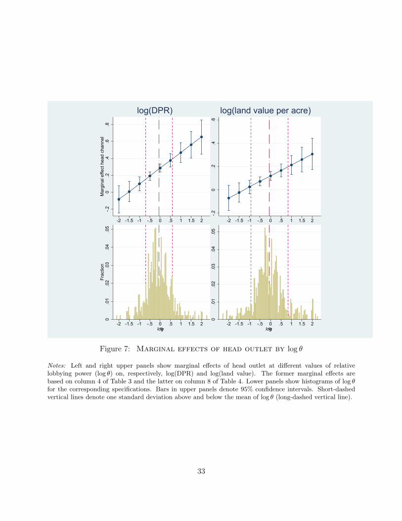
in Table 4 allow us to quantitatively assess the impact of a relative shift in lobbying influence
parameterized by θ = ιH/ιT . Looking across channels, there is near equality of influence be-
tween head and tail outlets, with a very slight advantage for the tail (see the log θ histograms
in the lower panels of Figure 7, with G as the 98th percentile). Now consider the predicted
effect of a shift in log θ by one standard deviation about its mean, as illustrated in the top
panels of Figure 7. Our estimates imply that such a shift in favor of the head coalition in-
creases the head-tail differential in DPR from a base of 27.2 (2.3) log points to 39.1 (4.3) log
points, whereas the equivalent shift in favor of the tail would bring this differential down to
15.4 (3.1) log points.30 At the same time, a one standard deviation shift in influence in favor
of the head would increase the head-tail land value premium from a base of 11.4 (1.8) log
points to 19.8 (3.6), whereas the equivalent shift in favor of the tail would virtually eliminate
the premium, bringing it down to 2.9 (2.8).31,32 Given the primacy of agricultural land in
29Indeed, the bootstrapped p-values are smaller than those of the conventional Wald test based on thecluster-robust variance-covariance matrix. Hansen’s statistic essentially uses the likelihood ratio principleand hence cannot be adjusted for clustering. One additional caveat, albeit probably a minor one, is thatHansen assumes a balanced panel, whereas our data are unbalanced due to varying numbers of outlets perchannel. It is unknown if Hansen’s results extend to our case.
30Standard errors in parentheses. Notice that, as a consequence of Jensen’s inequality, the mean percentagehead-tail differential in DPR is larger than the absolute differential as a percentage of mean tail DPR reportedin subsection 4.2.
31Recall that we are using a different γ for land values than for DPR (i.e., γ = 0.545 in the former caseversus γ = 0 in the latter case), which is why the scales of log θ are different.
32That the base head-tail land value differential of 11.4 log points is smaller than the corresponding DPRdifferential of 27.2 log points is consistent with the diminishing marginal product of water (concavity ofs(w)). In particular, log(VH/VT ) ≈ P (s − b)/(1 − P )s0 and log(wH/wT ) ≈ P w/(1 − P )w0. Now, s′′(w) =
32
-.20
.2.4
.6.8
Mar
gina
l effe
ct h
ead
chan
nel
-2 -1.5 -1 -.5 0 .5 1 1.5 2
0.0
1.0
2.0
3.0
4.0
5Fr
actio
n
-2 -1.5 -1 -.5 0 .5 1 1.5 2logθ
log(DPR)
-.20
.2.4
.6-2 -1.5 -1 -.5 0 .5 1 1.5 2
0.0
1.0
2.0
3.0
4.0
5
-2 -1.5 -1 -.5 0 .5 1 1.5 2logθ
log(land value per acre)
Figure 7: Marginal effects of head outlet by log θ
Notes: Left and right upper panels show marginal effects of head outlet at different values of relativelobbying power (log θ) on, respectively, log(DPR) and log(land value). The former marginal effects arebased on column 4 of Table 3 and the latter on column 8 of Table 4. Lower panels show histograms of log θfor the corresponding specifications. Bars in upper panels denote 95% confidence intervals. Short-dashedvertical lines denote one standard deviation above and below the mean of log θ (long-dashed vertical line).
33

the asset portfolio of most of rural Pakistan’s households, these hypothetical reallocations
of political power entail substantial redistributions of wealth along a channel.
5.4 Alternative explanations
One explanation of our findings is that the head-tail differential in lobbying influence as
measured by log θ is picking up something besides relative influence. In our regressions, we
control for several channel-level variables (Zc), including administrative division dummies,
that turn out to be highly correlated with head-tail differences in DPR and, to a lesser
extent, with head-tail differences in land values. Nonetheless, we may be omitting some
confounding variables. For instance, a large literature on collective action in commons man-
agement highlights the importance of heterogeneity among users (e.g., Ostrom 1990; Baland
and Platteau 1997), though the effect of this inequality on cooperative outcomes is often
theoretically ambiguous (Bardhan and Dayton-Johnson 2002). In the context of surface
irrigation systems, Bardhan (2000) and Dayton-Johnson (2000) provide evidence that the
landholdings Gini coefficient is negatively associated with cooperation in water allocation
and channel maintenance. The question here is whether log θ merely reflects land inequality
along a channel, vitiating our rent-seeking contest interpretation.
An immediate problem with the inequality story, however, is that, if there is a relationship
between log θ and the channel-level Gini coefficient, it is likely to be a U-shaped one. High
channel-level inequality should (mechanically) be associated either with high or with low
relative influence of the head outlets; low channel-level inequality should be associated with
more equal influence between head and tail outlets. This is exactly the pattern that we
observe in the data (Appendix Figure C.3). Hence, it comes as no surprise that controlling
for the channel-level Gini coefficient leaves our estimates of β1 virtually unchanged, as seen
in Table 5. Moreover, differences in the degree of land inequality on the channel as a whole
D′(w) < 0⇒ w/w0 > s(w)/s(w0)⇒ log(wH/wT ) > log(VH/VT ).
34

Table 5: Channel-level Inequality
Log(DPR) Log(land value per acre)
mean 98th percentile mean 98th percentile
β1 : H × log θ 0.213*** 0.185*** 0.0997*** 0.0928***(0.0520) (0.0455) (0.0291) (0.0314)
H× Gini 0.0229 0.0439 -0.165 -0.138(0.327) (0.309) (0.311) (0.330)
R2 0.642 0.643 0.781 0.781Observations 3,510 3,510 7,844 7,844
Notes: See notes to Table 2. Compare columns 1 and 2 to, respectively, columns 1and 4 of Table 3, column 3 to column 4 of Table 4, and column 4 to column 8 ofTable 4. Gini coefficient of family landholdings is computed at the channel level (i.e.,across head and tail outlets).
cannot explain variation in collective action or, rather, in its converse – water theft. This
finding is consistent with our presumption that cooperation between head and tail outlets
of a channel is practically nonexistent.
Another threat to our lobbying power interpretation revolves around the role of ground-
water. As suggested above, the market premium on land at the head of a channel is partly
attributable to better groundwater recharge at the head (due to more plentiful canal wa-
ter supplies). Recovering this groundwater, however, requires costly private investments
in tubewells. Only about a third of farmers in our data-set actually own a tubewell (or
tubewells) and ownership is heavily skewed toward the larger landowners; around half of all
tubewells are owned by the top 25% of farmers ranked by landholdings. Thus, one reason
why the head-of-channel premium is higher along channels with larger average landholdings
at the head might be that along these channels farmers at head outlets are better able to
exploit existing groundwater potential than those at tail outlets. In other words, our rela-
tive influence variable log θ may be picking up differential groundwater access. To address
this concern, which is obviously not relevant for DPR, we include the head-tail difference in
tubewell density (total number of tubewells per acre CCA), ∆TW/acre, in the land value
35

Table 6: Robustness Checks — Land Values
mean 98th percentile
β1 : H × log θ 0.114*** 0.0907*** 0.112*** 0.0816***(0.0294) (0.0347) (0.0321) (0.0309)
H ×∆TW/acre 1.732*** — 1.905*** —(0.593) (0.636)
H ×∆ logNC/acre — -0.0301 — -0.0331(0.0531) (0.0432)
R2 0.782 0.781 0.782 0.780Observations 7,844 7,798 7,844 7,798
Notes: See notes to Table 2. Dependent variable is log(land value per acre). Comparecolumns 1 and 2 to column 2 of Table 4, and columns 3 and 4 to column 8 of Table4. ∆TW/acre is the difference in no. of tubewells per acre cultivable command area( CCA) between head and tail outlets and ∆ logNC/acre is the difference in log no.of cultivators per acre CCA between head and tail outlets (available for 446 of 448channels, which accounts for 46 fewer observations in the corresponding regressions).
regressions (see Table 6). While this control attracts a significantly positive coefficient, so
that relatively greater access to groundwater does seem to enhance the head-of-channel land
value premium,33 the lobbying power effect is undiminished.
A final issue is that head-tail differences in the size distribution of family landholdings
may be correlated with head-tail differences in average land productivity, another example
of the potential incompleteness of Zc. There are three necessary elements to the argument,
each of which may be questioned: (1) substantial variation in average land quality between
head and tail outlets of the same channel; (2) larger returns to consolidating landholdings
in areas with higher average land productivity; (3) consolidation that mostly occurs through
land purchases. Under these conditions, we could observe larger landholdings on higher
productivity sections of the channel, thus reversing the arrow of causation relative to our
interpretation of the land value regressions (but, of course, not of the DPR regressions).
On element (1), we reiterate that median channel length (the maximum distance between
33It is also possible that this effect is not causal and that tubewell density is merely correlated with, e.g.,unobserved land productivity. The interpretation, however, is irrelevant for the robustness test.
36

head and tail outlets) is only 9 kilometers, which limits the extent of spatial variation in
land quality. On (2), there is no theoretical or evidentiary basis for the returns to scale
varying with land quality, although it is certainly a possibility. On (3), consolidation could
be achieved in part by one brother jointly managing his other brothers’ land, keeping family
landholdings (and, hence, log θ) constant or, similarly, through tenancy markets (leasing or
sharecropping), which are quite active in Pakistan. Note, as well, that according to the 2010
Agricultural Census, farmland purchases in Punjab over the previous 10 years amounted to
just 1.4% of total landownership.
These doubts aside, the differential returns to scale argument implies that the number
of cultivators per acre must be lower where land is more productive. Our survey records
how many cultivators (inclusive of pure tenant households) are at each outlet, from which
we can compute, except for two channels with missing values, the head-tail difference in
the (log) number of cultivators per acre CCA, ∆ logNC/acre. There is a strong negative
association between log θ and ∆ logNC/acre (see Appendix Figure C.4) — not surprisingly,
where average landholdings are larger there tend to be fewer cultivators per acre. However,
when we include ∆ logNC/acre in our land value regressions (Table 6), its coefficient is
insignificant, which suggests that returns to scale are not correlated with unobserved land
productivity differentials. Moreover, the estimates of β1 barely change. In sum, we find
support for our contention that the arrow of causation runs from differential influence to
land values, not the other way around.
5.5 Implications for inequality
Does variation in lobbying power exacerbate wealth inequality? We have already seen that
such variation can either reinforce or dampen wealth differences along a channel depending
on whether head or tail outlets have greater influence. Moreover, as indicated in Figure 7,
head and tail outlets have nearly equal lobbying power on the average channel (i.e., mean
37

0.2
.4.6
.81
cum
ulat
ive
prop
ortio
n of
land
wea
lth o
wne
d
0 20 40 60 80 100landownership percentile
current land prices counterfactual land prices
Figure 8: Rent-seeking and land wealth concentration
Notes: Counterfactual land prices zero out the effect of variation in log θ. Each point on the Lorenz curveindicates the cumulative proportion of land wealth owned by the households at or below a landownershippercentile. The solid curve is the 45 line of zero land wealth concentration.
log θ is quite close to zero). Here we consider the implications of rent-seeking for the overall
concentration of wealth.
We calculate land wealth by multiplying owned area by average land value on the outlet
for each of the roughly 220,000 individual farmers on the nearly 4,000 outlets. Figure 8
shows the Lorenz curve for land wealth at current land prices, indicating that the top 10%
of landed households own about half of land wealth.34 Next, we compute wealth at land
prices that net out the effect of log θ. In other words, in this counterfactual experiment, land
at head outlets with relatively high lobbying influence is assumed to be no more valuable
than land at head outlets with relatively low lobbying influence, and likewise for land at tail
outlets. As illustrated in Figure 8, the Lorenz curves for land wealth computed at current
and at these counterfactual land prices virtually coincide.
34While our sample is not necessarily representative of landowning households in Punjab province, letalone agricultural households overall, this is not critical for the illustrative calculations in Figure 8.
38

Since eliminating the return to rent-seeking, therefore, has a negligible impact on the
concentration of land wealth, we can conclude that variation in lobbying power does not
exacerbate overall inequality (even as it may do so along particular channels). While the
above-noted similarity of wealth distributions by location along a channel contributes to this
result, a more fundamental explanation is that the returns to lobbying for a common pool
resource are, in general, non-excludable. In our particular context, these rents accrue, not
only to the rich and powerful on an outlet, but also to their poor and powerless neighbors.
6 Conclusions
While optimal exploitation of common pool resources has received considerable attention
in economics, actual regulation of competing users on a commons has not. This paper
begins to fill this lacuna by studying bureaucratic canal management in the Indus Basin
watershed. Our theory of misgovernance views the irrigation administration as having to
mediate between contending coalitions of water-users along each channel. Supporting this
theory, we find that greater relative lobbying power – as measured by a novel index combining
economic stake and influential position-holding – enhances a coalition’s water allocation and
thereby redistributes wealth in its favor.
Looking beyond the Indus Basin, we suspect that similar mechanisms are at play in
other large state-managed irrigation systems and might explain why irrigation management
transfer, the devolution of authority to water-users groups, has not always been successful
(e.g., Meinzen-Dick 2007), a point elaborated on in Jacoby et al. (2018) in the context of
Pakistan’s own reform effort.
39

References
[1] Abadie, A., Athey, S., Imbens, G. W., & Wooldridge, J. (2017). When Should You
Adjust Standard Errors for Clustering? (No. w24003). National Bureau of Economic
Research.
[2] Acemoglu, D., & Robinson, J. (2008). Persistence of Power, Elites, and Institutions.
American Economic Review, 98(1), 267-293.
[3] Anderson, S., Francois, P., & Kotwal, A. (2015). Clientelism in Indian villages. American
Economic Review, 105(6), 1780-1816.
[4] Baland, J. M., & Platteau, J. P. (1997). Wealth inequality and efficiency in the commons
Part I: the unregulated case. Oxford Economic Papers, 49(4), 451-482.
[5] Baland, J. M., & Robinson, J. A. (2008). Land and power: Theory and evidence from
Chile. American Economic Review, 98(5), 1737-1765.
[6] Banerjee, A., Mookherjee, D., Munshi, K., & Ray, D. (2001). Inequality, control rights,
and rent seeking: sugar cooperatives in Maharashtra. Journal of Political Economy,
109(1), 138-190.
[7] Bardhan, P. (2000). Irrigation and cooperation: An empirical analysis of 48 irrigation
communities in South India. Economic Development and cultural change, 48(4), 847-
865.
[8] Bardhan, P., & Dayton-Johnson, J. (2002). Unequal irrigators: heterogeneity and com-
mons management in large-scale multivariate research. The drama of the commons,
87-112.
[9] Bandaragoda, D. J., & ur Rehman, S. (1995). Warabandi in Pakistan’s canal irrigation
systems: Widening gap between theory and practice. No. 7. IWMI.
40

[10] Bromley, D. W., Taylor, D. C., & Parker, D. E. (1980). Water reform and economic
development: institutional aspects of water management in the developing countries.
Economic Development and Cultural Change, 365-387.
[11] Burgess, R., Hansen, M., Olken, B. A., Potapov, P., & Sieber, S. (2012). The political
economy of deforestation in the tropics. Quarterly Journal of Economics, 127(4), 1707-
1754.
[12] Chakravorty, U., & Roumasset, J. (1991). Efficient spatial allocation of irrigation water.
American Journal of Agricultural Economics, 73(1), 165-173.
[13] Chambers, R. (1988). Managing canal irrigation: Practical analysis from south Asia.
New Delhi: Oxford.
[14] Dayton-Johnson, J. (2000). Determinants of collective action on the local commons: a
model with evidence from Mexico. Journal of Development Economics, 62(1), 181-208.
[15] Garces-Restrepo, C., Vermillion, D., & Muoz, G. (2007). Irrigation management trans-
fer: Worldwide efforts and results. FAO Water Report no. 32. Rome.
[16] Gisser, M. (1983). Groundwater: focusing on the real issue. Journal of Political Econ-
omy, 91(6), 1001-1027.
[17] Hansen, B. E. (1996). Inference when a nuisance parameter is not identified under the
null hypothesis. Econometrica, 413-430.
[18] Hansen, B. E. (1999). Threshold effects in non-dynamic panels: Estimation, testing,
and inference. Journal of econometrics, 93(2), 345-368.
[19] Huang, L., & Smith, M. D. (2014). The dynamic efficiency costs of common-pool re-
source exploitation. American Economic Review, 104(12), 4071-4103.
41

[20] Iyer, L., & Mani, A. (2012). Traveling agents: political change and bureaucratic turnover
in India. Review of Economics and Statistics, 94(3), 723-739.
[21] Jacoby, H., Mansuri, G., and Fatima, F. (2018). Decentralization and Redistribution:
Irrigation Reform in Pakistan’s Indus Basin. Policy Research Working Paper (forthcom-
ing). World Bank, Washington DC.
[22] Johnson, R. N., & Libecap, G. D. (1982). Contracting problems and regulation: the
case of the fishery. American Economic Review, 72(5), 1005-1022.
[23] Krueger, A. O. (1974). The political economy of the rent-seeking society. American
economic review, 64(3), 291-303.
[24] Lashari, B., Skogerboe, G. V., & Siddiqui, R. (1997). Hydraulic characteristics of pilot
distributaries in the Mirpurkhas, Sanghar and Nawabshah districts, Sindh, Pakistan.
Pakistan National Program, International Irrigation Management Institute.
[25] Meinzen-Dick, R. (2007). Beyond panaceas in water institutions. Proceedings of the
National Academy of Sciences, 104(39), 15200-15205.
[26] Mookherjee, D., & Png, I. P. L. (1995). Corruptible law enforcers: how should they be
compensated?. The Economic Journal, 145-159.
[27] Mustafa, D. (2002). Theory versus practice: the bureaucratic ethos of water resource
management and administration in Pakistan. Contemporary South Asia, 11(1), 39-56.
[28] Niehaus, P., & Sukhtankar, S. (2013). The marginal rate of corruption in public pro-
grams: Evidence from India. Journal of Public Economics, 104, 52-64.
[29] Nitzan, S. (1994). Modelling rent-seeking contests. European Journal of Political Econ-
omy 10, no. 1: 41-60.
42

[30] Olken, B. A. (2007). Monitoring corruption: evidence from a field experiment in In-
donesia. Journal of political Economy, 115(2), 200-249.
[31] Olken, B. A., & Barron, P. (2009). The simple economics of extortion: evidence from
trucking in Aceh. Journal of Political Economy, 117(3), 417-452.
[32] Ostrom, E. (1990). Governing the Commons: The Evolution of Institutions for Collec-
tive Action. New York: Cambridge University Press.
[33] Ostrom, E. & Gardner, R. (1993). Coping with asymmetries in the commons: self-
governing irrigation systems can work. Journal of Economic Perspectives, 7(4), 93-112.
[34] Qureshi, A. S., McCornick, P. G., Sarwar, A., & Sharma, B. R. (2010). Challenges and
prospects of sustainable groundwater management in the Indus Basin, Pakistan. Water
Resources Management, 24(8), 1551-1569.
[35] Ray, I., & Williams, J. (2002). Locational asymmetry and the potential for cooperation
on a canal. Journal of Development Economics, 67(1), 129-155.
[36] Reinikka, R., & Svensson, J. (2004). Local capture: evidence from a central government
transfer program in Uganda. Quarterly Journal of Economics, 119(2), 679-705.
[37] Rinaudo, J. D., Strosser, P., & Thoyer, S. (2000). Distributing water or rents? Ex-
amples from a public irrigation system in Pakistan. Canadian Journal of Development
Studies/Revue canadienne d’etudes du developpement, 21(1):113-139.
[38] Rinaudo, J. D. (2002). Corruption and allocation of water: the case of public irrigation
in Pakistan. Water Policy, 4(5), 405-422.
[39] Sampath, R. K. (1992). Issues in irrigation pricing in developing countries. World De-
velopment, 20(7), 967-977.
43

[40] Shleifer, A., & Vishny, R. W. (1993). Corruption. Quarterly Journal of Economics,
108(3), 599-617.
[41] Stock, J., & Watson, M. (2008). Heteroskedasticity-Robust Standard Errors for Fixed
Effects Panel Data Regression. Econometrica, 76(1), 155-174.
[42] Timmins, C. (2002). Measuring the dynamic efficiency costs of regulators’ preferences:
Municipal water utilities in the arid west. Econometrica, 70(2), 603-629.
[43] Tullock, G. (1980). Efficient rent-seeking. In Buchanan, J.; Tollison, R.; & Tullock, G.,
Toward a theory of the rent-seeking society, pp. 97-112.
[44] Van Waijjen, E. G., Hart, W. W. H., Kuper, M. & Brouwer, R. (1997). Using a hydro-
dynamic flow model to plan maintenance activities and improve irrigation water dis-
tribution: application to the Fordwah distributary in Punjab, Pakistan. Irrigation and
Drainage Systems 11, no. 4: 367-386.
[45] Wade, R. (1982). The system of administrative and political corruption: Canal irrigation
in south India, J. of Development Studies, 18(3): 287-328.
[46] Wittfogel, K. A. (1957). Oriental despotism: A study of total power. New Haven: Yale
University Press.
44

Appendix
A Proofs
Proof of lemma 1. Using equation (10) it is easy to show that b∗ > ∆s/2. Next,
differentiation of equation (10) yields
b∗θ = −rθ
[1− r + ∆s/2√
r(r + ∆s)
]. (A.1)
So, b∗θ > 0⇔√r(r + ∆s) < r + ∆s/2⇔ r + ∆s/2−
√r(r + ∆s) = b∗ −∆s/2 > 0.
Proof of Proposition 1. We have that τ ′(θ) > 0⇔ ∆w′
∆w− w′
T
wT> 0, where
∆w = wH − wT = P w, and also that ∆w′
∆w− w′
T
wT> 0⇔ P ′(θ) > 0, where
P ′(θ) ≡ Pθ + Pbb∗θ. (A.2)
FOC to problem (9) ⇒ Pb/P = −1/b∗, and Pb/P = −(1− P )Ωb/Ω = −(1− P )/(∆s− b∗),where the latter equality follows from the differentiation of Ω = ∆T/∆H . Finally,
Pθ = P (1− P )/θ. Inserting these results in (A.2) and rearranging yields
P ′(θ) =P (1− P )
θ
(1− θb∗θ
∆s− b∗
). (A.3)
Hence, P ′(θ) > 0⇔ ∆s− b∗ > θb∗θ. Using equation (A.1), we thus have that
τ ′(θ) > 0⇔√r(r + ∆s)− r > −r
[1− r + ∆s/2√
r(r + ∆s)
]⇔
r(r + ∆s) > r(r + ∆s/2)⇔
∆s > 0,
which is the condition for any theft to occur.
45

Proof of Proposition 2. We have that δ′(θ) > 0⇔ ∆V ′
∆V− V ′
T
VT> 0, where
∆V = VH − VT = P (s− b∗). Now,
∆V ′
∆V− V ′TVT
=P ′(θ)
P (1− P )− b∗θs− b∗
(A.4)
= 1− b∗θ[
1
∆s− b∗+
1
b∗(s− b∗)
]> 0⇔
b∗θ <(∆s− b∗)(s− b∗)∆s− b∗ + s− b∗
where the second line uses (A.3) and sets θ = 1. Since b∗ > ∆s/2,
(∆s− b∗)(s− b∗)s
<(∆s− b∗)(s− b∗)∆s− b∗ + s− b∗
.
Hence, it is sufficient to prove that b∗θ < (s− b∗)(∆s− b∗)/s. Using equation (A.1), this
condition can be shown, after some algebra, to be equivalent to
b∗ <
√s∆s
2. (A.5)
Next, we require that D(w) be linear, at least locally (i.e., on [w0, w]). Thus, letting
D(w) = d0 − d1w, where d0, d1 > 0 are parameters, we have w = d0/d1. Further, let
ρ = n/N = w0/w. We may now write s = d20/2d1, s0 = sρ(2− ρ), and ∆s = s(1− ρ)2.
Again with θ = 1, we also have
r =1− ρρ
s0 = s(1− ρ)(2− ρ).
Substituting these results into equation (10), we get
b∗ = s[3− 2ρ−
√(2− ρ)(3− 2ρ)
].
Since√s∆s = s(1− ρ), (A.5) amounts to 3− 2ρ−
√(2− ρ)(3− 2ρ) <
√1/2 or, after
more algebra,
h(ρ) = 2ρ2 +[7− 4(3−
√1/2)
]ρ− (3−
√1/2)2ρ2 < 0.
It is straightforward to verify that, indeed, h(ρ) < 0 for ρ ∈ [0, 1].
46

B Channel-Outlet Selection
B.1 Channels
From the universe of 2,978 channels with outlets:
1. Keep the 2,184 channels without off-taking minors or sub-minors.
2. Of these, keep 1,375 channels in areas that were not part of the irrigation reform.
3. Of these, keep 731 channels for which the total number of outlets is between the
median (9) and the 99th percentile (52), inclusive.
4. Of these, keep 518 channels having at least 4 outlets at head (top 40% by length) and
2 outlets at tail (bottom 20% by length).
5. Count the total number of channels per administrative division. Drop 8 divisions in
the lower quartile of the channel-count distribution to economize on visits to
divisional offices.
This leaves 470 channels across 24 divisions.
B.2 Outlets
The total number of outlets on these 470 channels is 9,614, of which 3,404 are at the head,
3,796 are at the middle, and 2,414 are at the tail.
1. Keep the first four outlets on the head of each channel (1,880 in total).
2. Keep all outlets on the tail (2,414).
This gives a total of 4,294 outlets.
47

C Additional Figures and Tables0
100
200
300
Freq
uenc
y
0 .8 2 3 4 5 6 7 8% influential families at head
010
020
030
0Fr
eque
ncy
0 .7 2 3 4 5 6 7 8% influential families at tail
010
020
030
0Fr
eque
ncy
0 .8 2 3 4 5 6 7 8% influential + police/army families at head
010
020
030
0Fr
eque
ncy
0 .7 2 3 4 5 6 7 8% influential + police/army families at tail
Figure C.1: Percentage of influential families by channel position
Notes: Top panel shows histograms of percentage of influential families (indicated by political, hereditary,irrigation department, or high civil positions) at the head (left) and tail (right) of 448 sample channels.Bottom panel changes definition of influential family to include members of the police and army. Verticallines indicates mean percentage across all channels (by position).
48

R2= 0.75
24
68
log(
98th
per
cent
ile o
f L1+
γI a
t hea
d)
2 3 4 5 6log(98th percentile of L at head)
R2= 0.75
24
68
log(
98th
per
cent
ile o
f L1+
γI a
t tai
l)
2 3 4 5 6log(98th percentile of L at tail)
Figure C.2: Unrestricted versus restricted (γ = 0) influence.
Notes: Regression of ιpc(0.545) on ιpc(0) (upper panel for p = H, lower panel for p = T ) using the 98thpercentile specification inclusive of army/police (N = 448).
49

0.2
.4.6
.8C
hann
el-le
vel l
and
Gin
i
-4 -2 0 2 4logθ
G = mean
0.2
.4.6
.8-4 -2 0 2 4
logθ
G = 98th percentilelog(DPR)
0.2
.4.6
.8C
hann
el-le
vel l
and
Gin
i
-5 0 5logθ
G = mean
0.2
.4.6
.8
-5 0 5logθ
G = 98th percentilelog(land values)
Figure C.3: Channel-level Gini coefficients and log θ
Notes: Nonparametric regression of the channel-level land Gini coefficient on log θ across 448 channels. Toppanels, from left to right, use the log θ in the DPR specifications with G = mean and 98th percentile, andwith γ = 0 in both cases. Bottom panels, from left to right, use the log θ in the land value specificationswith G = mean (γ = 0.815) and 98th percentile (γ = 0.545), and army/police included.
50

R2= 0.34
-50
5logθ
-2 0 2 4∆log(NC/acre)
Figure C.4: Relative influence and number of cultivators per acre
Notes: Regression of log θ from specification in column 2 of Table 4 on ∆ log(NC/acre), the head/taildifference in log number of cultivators per acre CCA (N = 446).
51

Table C.1: Selected Channel Characteristics by Administrative Division
No. of Median No. of Mean no. of Median no.selected channel selected selected outlets of irrigators
Division channels length (km) outlets Head Tail per outlet
Ahmedpur 16 8.9 144 3.9 5.1 73Bahawalpur 24 7.7 201 3.9 4.5 35Bhakkar 12 13.3 94 3.8 4.1 45Dallas 23 8.2 198 3.9 4.7 57Gujranwala 19 10.1 166 3.9 4.8 46Gujrat 12 9.6 90 4.0 3.5 65Kasur 13 10.8 104 3.9 4.1 69Khanpur 26 7.7 225 3.9 4.8 56Khanwah 27 8.5 238 3.9 4.9 36Khushab 13 14.1 111 4.0 4.5 36Kotadu 22 7.7 189 3.4 5.2 31Lahore 18 7.3 148 3.8 4.4 54Layyah 18 14.3 149 4.0 4.3 53Lodhran 21 11.9 199 3.9 5.6 68Mianwali 10 10.4 87 4.0 4.7 49Multan 23 10.9 213 3.9 5.3 48Muzaffargarh 36 9.2 344 3.9 5.7 49Pasrur Link 11 7.4 98 4.0 4.9 33Rahimyar Khan 30 8.4 261 3.9 4.8 50Sarghoda 11 8.8 80 3.6 3.6 45Sheikhupura 22 12.3 206 3.9 5.5 46Shujabad 15 7.3 126 4.0 4.4 42Suleimanki 11 8.5 87 3.6 4.3 61Trimmu Barrage 15 12.5 165 3.9 7.1 48
All sample 448 9.2 3923 3.9 4.9 47
Notes: Of the 470 intended channels, 1 could not be surveyed, 4 were permanently closed, 15 had noopen head outlets, and 2 had no open tail outlets, leaving 448 channels (3923 outlets) for the empiricalanalysis.
52