
gould moav selection july 2011 - University Of...
59
When is “Too Much” Inequality Not Enough? The Selection of Israeli Emigrants Eric D. Gould and Omer Moav ¤ October 3, 2011 Abstract This paper examines the e¤ect of inequality on the incentives to emigrate accord- ing to a person’s education and unobservable skills (residual wage). Borjas (1987) shows that higher skilled individuals are more likely to emigrate than lower skilled individuals when the returns to skill are higher in a potential foreign destination. Using a unique data set on Israeli emigrants, we show that the probability of emi- grating indeed increases monotonically with education. However, the relationship between residual wages and emigration rates exhibits an inverse u-shaped pattern. We build a model to explain both of these patterns by incorporating the idea that education is a “general” skill which can be transferred to a foreign country, but residual wages are composed of “general” and “country-speci…c skills” which are not easily transferable. We test the model’s predictions by exploiting variation in the patterns of emigration across industries and occupations. Our …ndings are consistent with the theory, and therefore, highlight the importance of di¤erentiating between general and “country-speci…c” skills in order to understand emigrant selection. ¤ A¢liations for the authors are: Eric Gould - Hebrew University, CEPR, and IZA; Omer Moav - Hebrew University, Royal Holloway University of London, and CEPR; Email addresses of the authors (respectively): [email protected], [email protected]. We thank Daniel Hamermesh for valuable comments, as well as seminar participants at the Hebrew University, Tel Aviv University, Bar Ilan University, the Labor Studies Workshop at the NBER Summer Institute, SOLE Meetings, University of Michigan, University of Rochester, the Berlin Network of Labour Market Research (BeNA), City University London, Warwick, Royal Holloway, and Ben Gurion University. We thank Shalva Zonenashvili for providing excellent research assistance, and …nancial support from the Maurice Falk Institute for Economic Research and the Pinhas Sapir Center for Development. 0
-
Upload
duongquynh -
Category
Documents
-
view
213 -
download
0
Transcript of gould moav selection july 2011 - University Of...

When is “Too Much” Inequality Not Enough?The Selection of Israeli Emigrants
Eric D. Gould and Omer Moav ¤
October 3, 2011
Abstract
This paper examines the e¤ect of inequality on the incentives to emigrate accord-ing to a person’s education and unobservable skills (residual wage). Borjas (1987)shows that higher skilled individuals are more likely to emigrate than lower skilledindividuals when the returns to skill are higher in a potential foreign destination.Using a unique data set on Israeli emigrants, we show that the probability of emi-grating indeed increases monotonically with education. However, the relationshipbetween residual wages and emigration rates exhibits an inverse u-shaped pattern.We build a model to explain both of these patterns by incorporating the idea thateducation is a “general” skill which can be transferred to a foreign country, butresidual wages are composed of “general” and “country-speci…c skills” which are noteasily transferable. We test the model’s predictions by exploiting variation in thepatterns of emigration across industries and occupations. Our …ndings are consistentwith the theory, and therefore, highlight the importance of di¤erentiating betweengeneral and “country-speci…c” skills in order to understand emigrant selection.
¤A¢liations for the authors are: Eric Gould - Hebrew University, CEPR, and IZA; OmerMoav - HebrewUniversity, Royal Holloway University of London, and CEPR; Email addresses of the authors (respectively):[email protected], [email protected]. We thank Daniel Hamermesh for valuable comments, as wellas seminar participants at the Hebrew University, Tel Aviv University, Bar Ilan University, the LaborStudies Workshop at the NBER Summer Institute, SOLE Meetings, University of Michigan, Universityof Rochester, the Berlin Network of Labour Market Research (BeNA), City University London, Warwick,Royal Holloway, and Ben Gurion University. We thank Shalva Zonenashvili for providing excellent researchassistance, and …nancial support from the Maurice Falk Institute for Economic Research and the PinhasSapir Center for Development.
0

1 Introduction
This paper uses unique data from Israel to examine the e¤ect of inequality on the incentives
to emigrate according to a person’s education and unobservable skills (residual wages). In
cross-country comparisons, Israel ranks among the countries with the highest levels of
income inequality in the developed world.1 In addition, recent evidence indicates that
Israel is su¤ering from a “Brain Drain” (Gould and Moav (2007) and Ben-David (2008)).
However, this paper examines the general idea that the existence of a brain drain is a sign
that inequality is too low, a prospect which is well-founded in economic theory.
A seminal paper by Borjas (1987) shows that higher skilled workers are more likely
than less-skilled workers to leave a country with a low return to skill and move to a country
with a higher return to skill.2 The reverse is also true – a lower skilled individual is more
likely than a higher skilled worker to leave a country with a high return to skill and move to
a country with a lower return to skill. These predictions are quite intuitive – higher skilled
individuals bene…t from higher inequality since they are at the top of the distribution,
while lower skilled individuals bene…t from lower inequality since they are at the bottom
of the distribution. Therefore, a more compressed wage distribution encourages higher
skilled individuals to leave (“positive selection”), while a more dispersed wage distribution
entices lower skilled individuals to leave (“negative selection”). Thus, attempts to lower
inequality may exacerbate the magnitude of a brain drain.
In this paper, we empirically and theoretically examine the selection of emigrants in
terms of their education levels and their unobserved skills, represented by an individual’s
residual wage (after controlling for education, age, etc.). Our theoretical contribution is to
extend the Borjas model by arguing that some skills are “general” in the sense that they can
be easily transported to a foreign country, and some skills are “country-speci…c” in nature,
and therefore, are not easily transferred to another country. Education is an example of a
“general skill” which is likely to be rewarded in any country, while examples of “country-
speci…c” skills include personal connections, local knowledge of the product and labor
markets, language-speci…c communication skills, legal knowledge of the local environment,
licenses which are country-speci…c, rents from union membership, …rm-speci…c skills, and
certain instances of luck (being at the right place at the right time).
1For example, Brandolini and Smeeding (2008) examine 24 developed countries and …nd that only theUnited States has a higher ratio of personal disposable income between the 90th and 10th percentiles.
2Borjas (1987) builds on the classic model of occupational choice by Roy (1951). Sjaastad (1962) alsomodels the decision to emigrate based on the wage gain net of migration costs.
1
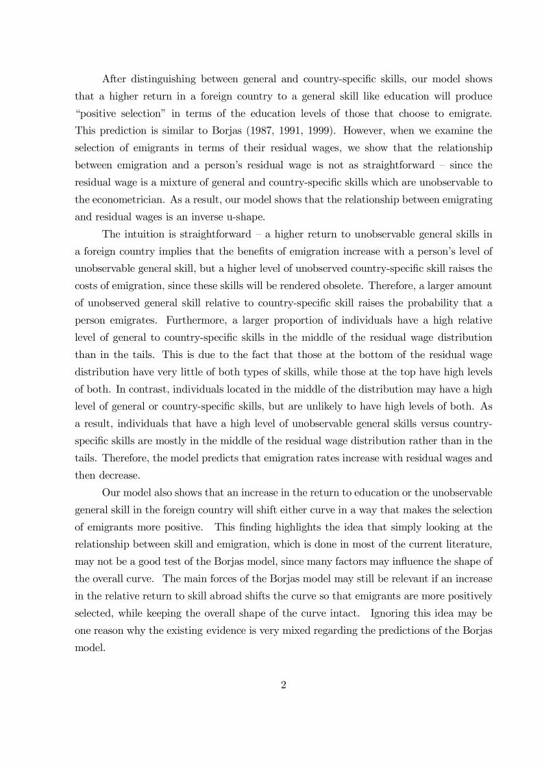
After distinguishing between general and country-speci…c skills, our model shows
that a higher return in a foreign country to a general skill like education will produce
“positive selection” in terms of the education levels of those that choose to emigrate.
This prediction is similar to Borjas (1987, 1991, 1999). However, when we examine the
selection of emigrants in terms of their residual wages, we show that the relationship
between emigration and a person’s residual wage is not as straightforward – since the
residual wage is a mixture of general and country-speci…c skills which are unobservable to
the econometrician. As a result, our model shows that the relationship between emigrating
and residual wages is an inverse u-shape.
The intuition is straightforward – a higher return to unobservable general skills in
a foreign country implies that the bene…ts of emigration increase with a person’s level of
unobservable general skill, but a higher level of unobserved country-speci…c skill raises the
costs of emigration, since these skills will be rendered obsolete. Therefore, a larger amount
of unobserved general skill relative to country-speci…c skill raises the probability that a
person emigrates. Furthermore, a larger proportion of individuals have a high relative
level of general to country-speci…c skills in the middle of the residual wage distribution
than in the tails. This is due to the fact that those at the bottom of the residual wage
distribution have very little of both types of skills, while those at the top have high levels
of both. In contrast, individuals located in the middle of the distribution may have a high
level of general or country-speci…c skills, but are unlikely to have high levels of both. As
a result, individuals that have a high level of unobservable general skills versus country-
speci…c skills are mostly in the middle of the residual wage distribution rather than in the
tails. Therefore, the model predicts that emigration rates increase with residual wages and
then decrease.
Our model also shows that an increase in the return to education or the unobservable
general skill in the foreign country will shift either curve in a way that makes the selection
of emigrants more positive. This …nding highlights the idea that simply looking at the
relationship between skill and emigration, which is done in most of the current literature,
may not be a good test of the Borjas model, since many factors may in‡uence the shape of
the overall curve. The main forces of the Borjas model may still be relevant if an increase
in the relative return to skill abroad shifts the curve so that emigrants are more positively
selected, while keeping the overall shape of the curve intact. Ignoring this idea may be
one reason why the existing evidence is very mixed regarding the predictions of the Borjas
model.
2

Our empirical analysis exploits a unique data set which includes the demographic
and labor force characteristics of a random sample of Israelis in 1995, combined with an
indicator for whether the respondent decided to emigrate as of 2004. This data set is a
rare opportunity to examine the selection of emigrants using information on the emigrants
before they move.3 Without information on wages before a person decides to move, it is
impossible to examine the selection of emigrants in terms of their residual wages (unob-
servable skill).
The basic patterns in the data support the main predictions of our model. Speci…-
cally, the probability of emigrating increases with education, which is consistent with the
model since the return to education in Israel is found to be much lower (0.071 versus
0.100) than the primary destination of Israeli emigrants, the United States. Also, the
overall relationship between residual wages and emigrating displays the inverse u-shaped
pattern which is predicted by our model. However, we also test the model further by
seeing whether the patterns of selection vary systematically with variation across di¤erent
sectors (industries and occupations) in the di¤erences between Israel and the United States
in the returns to observable (education) and unobservable skills. It is important to note
that we do not assume that all Israeli emigrants move to the US (although we show that
most of them do), nor do we assume that they do not change their industry or occupation.
Rather, the empirical strategy is to estimate to what extent Israelis consider these factors,
and whether they do so in a way that is consistent with the model.
Our …ndings strongly suggest that this is indeed the case: a lower return to un-
observable skill (proxied by the sector’s residual wage variance) in Israel versus the US
entices Israelis with higher residual wages to leave the country. Also, we …nd that emi-
grants are more positively selected in terms of their education in industries with a lower
relative return to education in Israel versus the US. The coe¢cient estimates are not only
statistically signi…cant, but also large in magnitude. For example, the estimates imply that
the positive relationship between emigration and education would be completely ‡attened
if the returns to education in each industry were equal in Israel and the United States.
Overall, this paper presents perhaps the strongest evidence in favor of Borjas (1987)
3Chiquiar and Hanson (2005) write on page 240: “Largely missing in the discussion of U.S. immigrationis evidence from source countries. Surprisingly, there is little work on how the skills of immigrants compareto the skills of nonmigrating individuals in countries of origin. Such data are essential to evaluate thenature of migrant selection.” Akee (2009) also utilizes labor market information on emigrants before theyleave from Micronesia. Consistent with our results, he …nds no linear e¤ect of household income on theprobability of emigrating, but does not examine whether the relationship is non-linear. Information onwages of movers before they move is more common in the internal migration literature ((Borjas, Bronars,and Trejo (1992), and Dahl (2002)).
3

regarding selection on education, and we are also the …rst to show that the forces of
the Borjas model hold for selection on residual wages, since an increase in the return to
unobservable skill abroad keeps the u-shaped pattern intact while shifting it to make the
selection more positive. Therefore, our …ndings highlight the importance of di¤erentiating
between general and “country-speci…c” skills in order to understand emigrant selection,
and imply that policies aimed at reducing inequality should focus on reducing the returns
to country-speci…c skills in order to minimize the e¤ect on the brain drain.
Although a few recent papers have examined the selection of emigrants according
to education and unobservable skill (see Akee (2010)), this is the …rst to test whether
variation in the returns to education and unobservable skill can explain the patterns of
emigrant selection on each dimension. Most of the literature examines the Borjas model
in terms of selection on education, with a large share dedicated to the selection of Mexican
immigrants to the US. According to the Borjas model, Mexican emigrants should be
negatively selected on education since the return to education is higher in Mexico than the
United States. The most prominent paper in this literature is Chiquiar and Hanson (2005),
who …nd evidence against the “negative selection” hypothesis for Mexican immigrants to
the United States.4 Instead, they …nd that Mexican immigrants to the US come from the
middle of the education distribution, which they explain by adding migration costs which
decline with education to the model.5 As a result, Mexican workers at the bottom of the
distribution are less likely to move due to their higher costs of moving, while those at the
top of the distribution are less likely to move due to the higher returns to education in
Mexico. In contrast, our results regarding selection on education are consistent with the
basic model with or without the assumption that migration costs decline with education,
and this additional assumption cannot help to explain the inverse u-shaped pattern we
see regarding selection on unobservable skill (residual wages). If we add moving costs
which decline with unobservable skill, this will only make those at the top of the residual
wage distribution even more likely to emigrate, when in fact, our goal is to explain why
those at the top have lower emigration rates than those in the middle of the distribution.
Therefore, the augmented model by Chiquiar and Hanson (2005) is useful in understanding
4Orrenius and Zavodny (2005) …nd similar results for illegal immigrants from Mexico. McKenzie andRapoport (2007) show that the selection of Mexican immigrants becomes more negative from areas inMexico which have lower overall migration costs (i.e. stronger migration networks).
5They argue that migration costs decline with education due to the e¤ect of education on the abilityto overcome bureaucratic requirements, the lower time costs required to earn enough money to pay the…xed-costs of moving, and fewer credit constraints on educated individuals. Chiswick (1999) also arguesthat moving costs decline with education, which tends to produce positive selection in emigrants.
4

Mexican immigration, but cannot explain the inverse u-shaped pattern we observe in our
data, thus underscoring the theoretical contribution of distinguishing between “general”
and “country-speci…c” skills in our model.
The literature on the selection of emigrants from countries other thanMexico presents
a mixed picture in terms of being consistent with Borjas (1987).6 This is largely due to the
general pattern whereby highly educated individuals leave less developed countries with
high returns to education and move to developed countries with lower returns to education.
This pattern is not consistent with the predictions of the basic model in Borjas (1987).
There may be many confounding factors in this type of empirical analysis, since there is
large variation across countries in many factors which may in‡uence the size and direction
of the selection – such as language barriers, proximity, moving costs, immigration policy,
visa requirements, etc. This may be one reason why the evidence in favor of the Borjas
(1987) model is stronger in studies looking at internal migration (Borjas, Bronars, and
Trejo (1992) and Dahl (2002)).
Our study is not a¤ected by cross-country di¤erences in factors which in‡uence the
selection of emigrants, since we exploit variation in the patterns of selection across sectors
within one country, rather than across countries. Moreover, we examine emigrant selection
based on education and unobservable skill (residual wages), and not just on education
which is the focus of the studies mentioned above.
The paper proceeds as follows. The next section describes our unique data and
presents the basic patterns of selection in terms of education and residual wages. Since
the pattern of emigrant selection on residual wages is inconsistent with the Borjas model,
Section 3 develops a model which can explain the observed patterns of selection on edu-
cation and residual wages. Section 4 tests the model’s predictions further by examining
whether variation in the relative (Israel versus the US) returns to education across sec-
6This literature includes Borjas (1987), who uses data on U.S. immigrants from 41 countries in the1970 and 1980 U.S. Censuses and …nds weak evidence that the source country’s income inequality isnegatively related to immigrant wages. Cobb-Clark (1993) …nds similar results for female immigrants.Feliciano (2005) examines 32 immigrant groups in the United States, and …nds that all but one group(immigrants from Puerto Rico) are positively selected in terms of education. However, Feliciano (2005)…nds an insigni…cant relationship between inequality and the degree of positive selection from the sourcecountry. Grogger and Hanson (2011) examine the sorting of immigrants to 15 OECD countries from 102source countries and …nd that immigrants in host countries are positively selected in relation to the sourcecountry when the education gap in wages between the host and source countries increases. However, whenthe education wage gap is measured in logs, they …nd evidence in favor of negative selection when thereturn to education is higher in the source country. Belot and Hatton (2008) examine immigrants in 29OECD countries from 80 source countries and …nd little evidence in favor of the main prediction in Borjas(1987). Only after considering the poverty constraints in poor countries do they …nd evidence in supportof Borjas (1987).
5

tors can explain variation in the patterns of emigrant selection across sectors. Section
5 presents a similar analysis of emigrant selection on residual wages. Section 6 presents
some robustness checks. Section 7 discusses the magnitude of the coe¢cients and Section
8 concludes.
2 The Data
The analysis uses a unique data set composed of the 1995 Israeli Census merged with
an indicator for whether each respondent left the country or not as of 2002 and as of
2004. (We also received an indicator for whether the person died by 2002 or 2004.) If the
person is considered a “mover” (a person who has left Israel), then the data set contains
variables indicating the month and year when this person is considered to have left the
country permanently. Information on whether the person left the country is obtained by
the Israeli border police, which closely monitors who is coming and going at the country’s
points of entry and exit. Therefore, one advantage of this data is that we do not have
to worry about counting illegal immigrants, which is typically very di¢cult to do using
governmental data in the host country (see Hanson and Spilimbergo (1999) and Hanson
(2006)).
De…ning who is an emigrant is not straightforward. Many individuals travel abroad
intending to stay for only a short period of time, but gradually their stay becomes per-
manent. Others may intend to leave forever but change their mind. As a result, any
de…nition of a “mover” is somewhat arbitrary. In our analysis, we use the o¢cial de…ni-
tion used by the Israel Central Bureau of Statistics, which considers any individual as a
“mover” if he/she left the country for at least a full year.7 By design, the variable for being
a “mover” is intended to capture a long-term absence from the country. According to the
algorithm used by the Central Bureau of Statistics, a short visit back to Israel in the midst
of a long-term absence does not change the status from “mover” to being a “non-mover.”
There are a few potential weaknesses of the data worth noting. First, the data set
does not indicate why a person leaves and whether the person intends to come back or not.
The person may not know this information himself. Therefore, although we mainly use
the given measure of a “mover” throughout our analysis, we check the robustness of our
results by classifying only longer-term movers as “movers” (using the information about
7The Israel Central Bureau of Statistics received information from the Interior Ministry about whois leaving the country, which the Interior Ministry collects at the airports and borders according to thepersonal identi…cation number.
6

when the person moved). In addition, as we discuss below, there is strong evidence to
believe that the measure we received is picking up moves which are indeed long term. A
second weakness in the data is that it does not contain information on where the person is
living if he/she resides outside of the state of Israel. However, the Global Migrant Origin
Database Version 4.0 indicates that the United States is by far the most likely destination
for Israeli emigrants.8 Therefore, we treat the United States as the “host” country of
interest. To the extent that the United States is not the actual destination for a particular
emigrant, this should only add noise to the analysis.
Descriptive statistics for the main variables of interest from the 1995 Israeli Census
are presented in Table 1. Since the focus of the paper is to determine the selection of
emigrants in terms of their education and wages, we restrict the analysis to males with a
strong attachment to the labor force, who are old enough to …nish their schooling (Israelis
typically start their BA studies at 22-24 years old) but young enough so that they are
not leaving for retirement purposes. Speci…cally, we restrict the sample to Jewish males
between the ages of 30 and 45 who were not self-employed (so their income measure is
reliable), worked at least 30 hours a week, worked at least six months in the previous year,
and are not ultra-orthodox.
Table 1 shows that the overall rate of emigration as of 2004 in this sample stands at
1.6 percent. The rate as of 2002 was 1.3 percent, so there appears to be an increase over
time. Over 67 percent of those characterized as “movers” in 2004 emigrated by the end of
2000. In addition, only two percent of those characterized as a “mover” in 2002 returned
to Israel by the end of 2004. So, our measure of a “mover” appears to be picking up longer
term stays abroad. Table 1 also contains means for the other variables used throughout the
analysis: education (13.0 years of education), age (37.7), native (61.4 percent were born
in Israel), marital status (90 percent married), number of children (2.13), and monthly
wages.
Although the overall rate of emigration appears to be rather low at 1.6 percent,
there are stark di¤erences across levels of education and wages. Figure 1a presents the
rates of emigration across di¤erent levels of education. The rate for those with a high
school education or less is about 1.1 percent, but the rate increases signi…cantly for college
8The data in the Global Migrant Origin Database Version 4.0 is problematic since it is based on countryof birth, and many Israelis were not born in Israel. Also, it does not distinguish between Jewish and ArabIsraelis, while this study focuses on the emigration status of the Jewish population. However, according tothe database, 122,591 Israelis moved to the US and the next highest country (excluding Arab countries) isCanada with a total of 17,393. Therefore, the United States is by far the most likely destination country.
7

graduates to 1.6 percent, and then jumps dramatically for those with an MA degree or
higher to 4.6 percent. The high emigration rate for the most educated Israelis has raised
concerns within Israel about a signi…cant “brain drain.” Figures 1a and 1b show similar
patterns for natives and non-natives, but the magnitudes are much higher for non-natives.9
It is worth noting that these patterns are not due to restricting our sample to those above
the age of 30, which could lead to a similar pattern if less-educated Israelis tend to leave in
their 20’s while more educated individuals wait until they …nish schooling. Figure 2a shows
that the probability of emigrating increases with education even for those in their 20’s.
In addition, Figure 2b shows that emigration rates by 2004 for teenagers in 1995 increase
with their father’s education level. Therefore, all the evidence suggests that emigrants
are indeed positively selected according to family background and education during their
teenage years and into their mid-40’s.
The positive relationship between education and the rate of emigration is consistent
with the predictions of the Borjas model. Speci…cally, the Borjas model predicts that the
propensity to emigrate should increase with education in a country with a low return to
education in comparison to a potential host country. Indeed, conventional OLS estimates
of the returns to education in Israel are quite low. Table 2 presents Mincer-like wage
regressions using data from the US and Israel from the same period and using similar
sample selection criteria. The estimated return to education is 10.0 percent for the US and
only 7.1 percent for Israel. This di¤erential is likely to be a factor which is generating the
positive relationship between education and emigration in Figures 1a and 1b. It is worth
noting that this relationship is positive and signi…cant after controlling for a host of other
demographic characteristics of the individual, as shown in a regression in the third column
of Table 2.
However, one potential explanation for the pattern exhibited in the …gures could be
that individuals with higher education levels are more likely to spend time temporarily
abroad (sabbaticals, being stationed abroad by a …rm or the government, etc.). However,
we …nd no evidence to support this idea. Figure 3 shows that there is no discernible
relationship between education and the propensity to return between 2002 and 2004, given
that you were considered a “mover” in 2002. The last column of Table 2 con…rms that there
is no systematic pattern between “returning” and education levels even after controlling
for other demographic characteristics and wages. Therefore, we believe that the patterns
9Gould and Moav (2007) show that the rate of emigration is very high for professors, scientists, doctors,and engineers. All of these groups are at least three times higher than teachers or workers in all the restof the occupations.
8

in the data are unlikely to be picking up the tendency for highly educated individuals to
work for a year or two abroad.10
However, the increasing likelihood of higher educated individuals to emigrate could
possibly be explained by other factors. For example, the costs of obtaining a work visa
or …nding a job abroad may decline with education. Therefore, variation in the relative
returns to education is needed to truly test the predictions of the Borjas model. To do
this, we estimate the returns to education within sectors in the United States using the
same speci…cation used in the …rst column of Table 2, and within sectors in Israel using
the speci…cation in second column of Table 2. Table 3 presents the estimated returns
to education in the US and Israel when the sectors are de…ned by industry, and Table 4
presents the estimates when the sector is de…ned by occupation. In our main empirical
analysis, we will exploit variation in the relative returns to education (Israel versus the
US) across sectors to test the predictions of Borjas model regarding the selection of Israeli
emigrants from each sector.
Although most of the literature examining the Borjas model looks at whether there is
a positive or negative selection of emigrants according to their education (observable skills),
the model in Borjas (1987) also applies to unobservable skills. We measure the returns
to unobservable skill with residual inequality (see Juhn, Murphy, and Pierce (1993)). The
…rst two columns in Table 2 show that the residual variation is higher in the US versus
Israel, after controlling for a similar set of demographic characteristics. Speci…cally, the
“Root MSE” from the Mincer-like wage regression is 0.523 for the US and 0.498 for Israel.
According to the Borjas model, the higher return to unobservable skill in the US should
entice individuals with higher residual wages to emigrate. However, a simple descriptive
analysis is not consistent with this prediction. The third column in Table 2 shows that
wages are not a signi…cant predictor of who moves, and Figure 4 shows that the propensity
to emigrate increases with residual wages and then declines. That is, it is not the case that
no pattern exists at all between residual wages and the propensity to leave Israel. Rather,
the pattern is non-linear – characterized by an inverse U-shape. Apparently, individuals
with very low residual wages and very high residual wages are less likely to emigrate than
those in the middle of the distribution, which is not consistent with a simple Borjas model.
As shown in Figures 5 and 6, this pattern persists even after controlling for twelve industry
10We abstract from the issue of return migration (see Dustmann (2003) and Dustmann and Weiss(2007)). However, Table 1 shows that only two percent of those that were considered movers in 2002moved back by 2004. Given this low number of returning Israelis and the …nding that they are notdisproportionately educated (as noted above), we focus exclusively on the selection of the moving decision.
9

categories or eight occupation groups.
Chiquiar and Hanson (2005) also found that, in contrast to the predictions of the
Borjas model, emigrants from Mexico come from the middle part of the education distri-
bution rather than being concentrated in the lower tail (since the returns to education in
Mexico are higher than they are in the US). They reconciled their …ndings by including
in the Borjas model a cost of emigration which declines with education. Therefore, they
explain the lower rate of emigration by low educated workers in Mexico by their high costs
of moving, and the lower rate of emigration of highly educated workers by the higher re-
turn to education in Mexico. Our case is obviously di¤erent, since our evidence regarding
the nature of the selection on education (observable skills) is entirely consistent with the
Borjas model with or without including a cost of emigration which declines with education.
More importantly, the adapted model by Chiquiar and Hanson (2005) cannot explain the
inverse U-shape in our data regarding unobservable skills – moving costs which decline
with residual wages would make those at the top of the residual wage distribution the
most likely to leave the country, whereby we are trying to explain why those in the middle
leave at the highest rates. Our …nding that those at the top do not leave at high rates may
be due to the idea that some factors of their success are unlikely to be transported to the
US.
In the next section, we formally show that incorporating the idea that some skills are
“country-speci…c” into the model can generate the inverse U-shaped relationship between
residual wages and the likelihood of emigrating. In this sense, the U-shaped pattern is
consistent with our model, but it may also be the result of unobserved factors. Again,
variation in the returns to unobservable skill is needed to test the implications of our model,
and for this purpose, we estimate the returns to unobserved skill in each sector using the
same set of regressions within each sector described above regarding the estimation of the
rates of return to education in each sector. The “root mean squared error” from each
regression is the estimated return to unobserved skill in each sector in the US and Israel,
and Tables 3 and 4 present these estimates for the di¤erent industries and occupations. In
our main empirical analysis, we will exploit variation in the relative returns to unobservable
skills (Israel versus the US) across sectors to test the predictions of our model regarding
the nature of the selection of emigrants with regard to unobservable skills.
10

3 AModel of Emigration with Country-Speci…c Skills
In this section, we present a model of the emigration decision which considers the idea that
some skills are “general” in the sense of being rewarded highly in a foreign country, while
some are not valued much at all in a foreign country, and therefore, are more “country-
speci…c” in nature. A signi…cant portion of an individual’s total human capital is likely to
be country-speci…c for several reasons. First, any skill which is “…rm-speci…c” is likely to be
country-speci…c as well. Second, language and cultural barriers may prevent an individual
from transferring their skills to a country where they lack a commanding knowledge of
the local language, cultural of business practices, consumer tastes, laws, and regulations.
Third, if a person’s success is at least partially due to luck (being in the right place at
the right time), good luck may not be transferable abroad. Fourth, many individuals with
high incomes became successful due to personal connections with local individuals and
authorities, and these connections will not be useful in a foreign country. For these and
other reasons, it is very likely that some people will not be able to translate their success
to a foreign country.
The model consists of individuals living in the source country (country 0) and decid-
ing whether or not to emigrate to the host country (country 1). An individual’s wage in the
source country, 0 is determined by his level of education, and by his unobservable (to
the econometrician) skills. Unobservable skills are composed of skills which are country-
speci…c, , and skills which are more general, . Following the literature, education is
considered a general skill which is also observable. An individual’s wage, 0 in the source
country is modeled by:
0 = 0 + + + (1)
where 0 is the intercept of the wage function and is constant across individuals. Without
loss of generality, the returns to each type of skill (, , and ) are normalized to one in
country 0 The two unobservable components, and are distributed independently with
a uniform distribution over the unit interval,
~ [0 1];
~ [0 1]
Using the uniform distribution simpli…es the analysis, but is not crucial for the qualitative
results. In Appendix Figures 1-3, we present simulations that show that the main results
11

hold for the normal distribution and when we allow for a negative or positive correlation
between and .
If an individual chooses to emigrate to the host country (country 1) he will receive
the following wage (net of the direct cost of moving to another country),
1 = 1 + 1+ 1 ¡ (2)
where 1 is the intercept of the wage function in country 1 1 and 1 are the returns to
and in country 1 and is the direct cost of relocating which is considered identical across
all individuals.11 Although several papers model the cost of moving as a decreasing function
of education (Chiswick (1999) and Chiquiar and Hanson (2005)), adding this element to
the model will only strengthen the results for positive selection on education, but would
not enable us to understand the inverse u-shaped pattern of emigration rates according to
residual wages, as depicted in the preceding section.12 The key assumption of the model
is that some skills are valued much more in the source country versus the host country,
which we simplify in the model by setting the return to unobserved country-speci…c skills,
to zero in country 1.
We restrict our analysis to the case where the returns to education and general
skills are higher in the host country versus the source country, since Section II shows that
this appears to be the case for Israelis who are considering a move to the United States.
Formally, this assumption is represented by 1 ¸ 1 and 1 ¸ 1
Following the framework developed by Roy (1951) and Borjas (1987), the decision
to emigrate is based on wage maximization. Therefore, individuals emigrate if and only
if 1 0 Based on equations (1) and (2), this condition holds if and only if:
+ + (3)
where = (0¡ 1)+ is the total …xed-cost of emigration (the di¤erence in the constant
plus the direct cost of relocating), = 1 ¡ 1 ¸ 0 and = 1 ¡ 1 ¸ 0 The parameters
11Hamermesh and Trejo (2010) show that there are …xed time-costs of assimilation for immigrants inthe host country.
12The other papers use the declining costs of emigration to explain why emigrants are not negativelyselected when the return to education in the source country (Mexico) is higher than the return in thehost country (United States). Since the returns to education are lower in Israel versus the United States,adding this element to the model only reinforces the positive selection of Israeli emigrants in terms ofeducation. Formally, making the direct cost relocating, a function of education or general skills, isequivalent to a change in the di¤erence in the relative returns to education or general skills between thetwo countries. This has no qualitative impact on the model, unless the cost is increasing with skill and/oreducation in a rate that can reverse the direction of the di¤erence. However, given the literature whichargues that the costs decline with skill, this possibility is not very reasonable.
12

and are the di¤erences in the returns between country 1 and country 0 to education and
general skills respectively. Hence, the right hand side of equation (3), + is the total
emigration cost including the loss of speci…c skills, whereas the left hand side, +
is the gain from emigration. Naturally, an individual decides to emigrate if the gain is
greater than the costs.
As stated above, an individual’s unobservable component of income in country 0 is
represented by + . This sum is called the individual’s “residual wage,” and is denoted
by ~ i.e.,
~ = +
Since both and are distributed uniformly over the unit interval, it follows that the
residual wage, ~ is distributed between 0 and 2. In order to focus the model on the most
realistic range of results, a few restrictions on the parameters are useful. In particular, we
restrict the parameters so that not everyone emigrates. Since the returns to education,
and general skills, are higher in country 1, individuals with a high level of and are
the most likely to gain from emigration. Equation (3) formally illustrates this point, as
the bene…ts of emigration increase with both and . Therefore, in order to ensure that
not everyone emigrates, we assume that for any individual characterized by the minimum
levels of education and general skills ( = = 0) the return to emigration is negative,
1 0 (If this holds, then it holds for any level of as well.) Formally, we assume that:
0 (A1)
so that condition (3) does not hold for any individual characterized by = = 0 regardless
of . Assumption A1 implies that a positive total …xed-cost of emigrating, represented by
causes those with the least to gain from emigration to choose not to emigrate.
Next, we focus on a di¤erent set of individuals who are very unlikely to emigrate –
those with low education and high country-speci…c skills. The condition in equation (3)
shows that the net bene…ts of emigration increase with and decline with – the latter
result stemming from the high loss of country-speci…c skills should the individual choose
to move. The only reason individuals with low and high would ever choose to emigrate
is because the return to is extremely high in country 1. Therefore, to preclude this
unreasonable case, we restrict the return to in country 1 to be no more than double the
13

return to in country 0. Formally, we assume that:
1 (A2)
which assures that equation (3) does not hold for any individual with = 0 and = 1
regardless of .
Although low educated individuals are the ones most likely to stay, we do not restrict
all of them to do so. In fact, we restrict the parameters so that not everyone with the
lowest education chooses to stay. In particular, for an individual with the lowest education
( = 0), equation (3) holds if + , which is most likely to be satis…ed if is high
and is low. Therefore, we assume that the return to is su¢ciently high so that:
(A3)
assuring that condition (3) holds for an individual with = 1 and = 0 regardless of
(as long as ¸ 0).
We now derive the probability of emigration for any individual with a given level
of education and a given residual wage, ~. We condition on these two variables since
these are observable to the econometrician, while the individual components of the residual
wage, and , are not observable. Since the distributions of and are uniform and
independent, it follows that for any given ~ is uniformly distributed in its feasible
range.13 In particular, the conditional distribution of given ~ is given by:
~ [0 ~] ~ · 1;~ [ ~ ¡ 1 1] ~ ¸ 1
These properties allow for a straightforward calculation of the probability that an indi-
vidual with any given ~ and will emigrate, which we denote by ( ~; ) As follows from
equation (3) and noting that = ~ ¡ ( ~; ) is given by:
( ~ ) ´ ( + + j ~) (4)
=
µ
¡ + ~
1 +
¯¯ ~¶
We further suppose that is su¢ciently large relative to so that the distribution
of is bounded from above by This implies that the return to education in country 1
versus country 0 is not so large that a majority of highly educated people decide to emigrate.
13Note that the probability that + 2 ( ¡ + ) for ! 0 for any given such that ~ ¡ 1is independent of and therefore the conditional probability of and for any given ~ are uniform in thefeasible range.
14

(This coincides with the case of Israel – the highest emigration rates are for those with
MA degrees, but the rate is still only 4.6% over the seven-year period we study.) This
assumption implies that the residual wage, and not just the level of education, plays an
in‡uential role in the decision to emigrate. Our assumption that is bounded from above
by implies that ¡ 0.14 All proofs are in the appendix.
Proposition 1 (The properties of ( ~ )) Under Assumptions A1-A3 and as long as
¡ 0
1. The probability that an individual decides to emigrate is:
( ~ ) =
8>>>><>>>>:
0 ~ · ¡
+1¡ ¡
(1+) ~ ~ 2
³¡
1´
1+¡(¡)¡ ~(2¡ ~)(1+)
~ 2 [1 1 + ¡ (¡ ))
0 ~ ¸ 1 + ¡ (¡ )
(5)
where,
2. ( ~ ) is continuous
3. ¡2 (0 1)
4. 1 + ¡ (¡ ) 2 (1 2)
5. (1 ) 2 (0 12)
6. ( ~ ) is increasing and concave with respect to ~ for ~ 2³¡
1´
7. ( ~ ) is decreasing and concave with respect to ~ for ~ 2 (1 1 + ¡ (¡ ))
According to Proposition 1, the probability to emigrate is an inverse u-shaped func-
tion of the residual wage, ~ if and are not too high and is su¢ciently high. The
intuition is rather straightforward. Generally speaking, individuals with a low residual in-
come have low levels of both general and country-speci…c skills ( and ). A low implies
that the individual has a limited incentive to emigrate in order to enjoy the higher return
to in country 1, while a low means that he will su¤er a small loss in terms of losing his
country-speci…c capital if he moves. These e¤ects o¤set each other, so that the net gain to
emigration for this individual is modest, and therefore, he will tend not to emigrate due to
the signi…cant …xed-costs of emigration, . On the other end of the spectrum, individuals
with very high residual wages will tend to have high levels of general and country-speci…c
skills. For these individuals, a high level of implies a larger bene…t to emigrating, while
a large means that he will su¤er a severe loss of country-speci…c skills. That is, similar
14We brie‡y discuss below the case where ¡ 0
15

to the individual with a low residual wage, the ratio of to is close to one, and therefore,
the costs and bene…ts of emigration roughly cancel each other out. As a result, a signi…-
cant level of …xed emigration costs will prevent individuals with a high residual wage from
leaving the country in large numbers.
Now, consider those in the middle of the residual wage distribution. In this range,
individuals have varying levels of and . Those with high levels of versus will behave
similar to those at the tails of the distribution since the loss of country-speci…c skills and
the …xed-costs will prevent them from leaving at a large rate. However, in the middle of
the distribution, there is a signi…cant group of people with high levels of relative to ,
and for those individuals, the return to emigration is high enough to produce the largest
rate of emigration within the population. As a result, the rate of emigration tends to be
larger in the middle of the residual wage distribution than in the tails.15
It is important to note how our results di¤er from the existing framework developed
by Borjas (1987). In his model, the selection of immigrants in terms of “unobservable
skill” is signi…cantly in‡uenced by the correlation of unobservable skills in the source
and host countries. Our model is di¤erent since the correlation between an individual’s
unobservable skill in both countries is di¤erent across people, rather than being a single
parameter. In particular, due to the variation in the level of country-speci…c skills across
people, some individuals stand to lose a large portion of their total unobservable skill
and some would lose virtually nothing. That is, our model produces a di¤erent rate of
transferability of unobservable skill across people according to the relative size of each
component of unobservable skill. By showing that a larger proportion of individuals with
a higher transferability rate of unobservable skills (i.e. those with a high relative to
) exists in the middle of the distribution of total unobservable skill (i.e. the residual
wage), our model is able to explain the inverse u-shaped pattern of emigration in relation
to unobservable skill.
We now examine the e¤ect of education on the shape of the probability function of
emigrating, ( ~ ).
15It should be noted that the inverse u-shaped relationship between the residual wage and the probabilityof emigration does not depend on our assumption that the two components of the residual, and areuncorrelated. The u-shape patterns persists for any type of correlation except for the case where they areperfectly, positively correlated (which would produce positive selection). However, the u-shaped patternbecomes ‡atter when the correlations becomes more positive. Interestingly, a negative correlation willstrengthen the inverse u-shape pattern, since a more negative correlation would increase the variance inthe distribution of and in the middle of the distribution of their sum, and hence a higher probabilityof exceeding its threshold level for triggering emigration. Also, it is worth noting that the results dodepend on the relative variances of and .
16

Proposition 2 (The e¤ect of on ( ~ ))Under Assumptions A1-A3 and as long as
¡ 0
1.( ~ )
0 ( ~ ) 0
2.2( ~ )
~ 0 ~ 2
µ¡
1
¶
3.2( ~ )
~ 0 ~ 2 (1 1 + ¡ (¡ ))
Part 1 of Proposition 2 implies that the probability of emigrating increases with the
level of education. In other words, emigrants are positively selected in terms of their
education, which follows from the higher return to education in country 1 versus country
0, 0. This result and its mechanism is similar to the prediction in Borjas (1987).
However, Proposition 2 demonstrates that the marginal e¤ect of on is decreasing with ~
for ~ 1 (part 2) and increasing with ~ for ~ 1 (part 3) That is, the inverse u-shaped
pattern of ( ~ ) with respect to ~ is shifting up and ‡attening out as increases.
For the case where ¡ 0 the results are generally in the opposite direction:
( ~ ) = 1 for both high and low levels of ~ and the lowest value of ( ~ ) is in the
middle of the distribution of ~ ( ~ = 1) Since this pattern is not observed in the data, we
focus our analysis on the case where ¡ 0
We now examine how the pattern of emigration across di¤erent levels of ~ changes
as the return to increases in country 1.
Proposition 3 (“mean preserving spread”) A rise in the return to unobservable general
skills in the host country versus the source country, and in the …xed cost of emigrating,
such that (1 ) is held constant, generates a decline in ( ~ ) for ~ 1 and a rise in
( ~ ) for ~ 1
It follows from Proposition 3 that a rise in while holding (1; ) constant, generates
a shift to the right in ( ~; ) around the point (1; ) In other words, a higher relative
return to unobservable general skills in country 1, while holding (1; ) constant, maintains
the overall u-shaped pattern of emigration according to residual wages, but shifts the whole
17

curve to the right (raising emigration rates for those with high residuals and lowering the
rate for low residual wages).
The intuition for this result is as follows. For a given the decision to emigrate
depends on both and The bene…ts of emigration increase with while the costs
increase with Therefore, as ~ increases, the sum of and increases, which implies that
the threshold level of above which individuals choose to emigrate, increases with ~ To
derive this formally, the condition for a person with any given ~ to decide to emigrate,
given by equation (3), can be re-written as,
+ + ~ ¡
where ~ ¡ = Re-arranging implies: + (1 + ) + ~ and therefore, for any ~
and , there exists a threshold level of denoted by ( ~ ) such that equation (3) holds
with equality:
( ~ ) =¡ + ~
1 +
Hence, the threshold level of is increasing with ~ and therefore a rise in the di¤erence
in the return to general skills, has a stronger impact on individuals with larger residual
wages, ~ This can also be seen from equation (3), where the marginal bene…t of emigrating
with respect to is equal to . Therefore, those with higher are more sensitive to changes
in This general result is independent of the speci…c “mean preserving spread” exercise
performed in the proposition.16
We now examine how the positive selection of emigrants, as shown in Proposition
2, is a¤ected by changes in the relative returns to education between the two countries.
To do this, we derive the probability of emigrating as a function only of education, and
discuss its properties.
Proposition 4 (the e¤ect of education on the emigration probability) Under A1-A3, for
0:
1. The probability of emigrating as a function of education is:
() =( ¡ + )2
2 0
16A rise in the …xed cost, has a negative e¤ect on the emigration probability. However, this e¤ectdeclines (in absolute value) with ~ for ~ 1 in particular, for ~ 2
³¡ 1
´ 2( ~) ~ = 1
~2(+1) 0For
~ 1 the opposite is true. For ~ 2 (1 1 + ¡ (¡ )), 2( ~) ~ = ¡ 1
(+1)(¡2)2 0
18

2. The probability of emigrating is an increasing and convex function of education:
()
=
( ¡ + ) 0
2()
2=
2
0
3. The probability of emigrating as a function of education increases and becomes
steeper with an increase in the return to education in country 1 relative to country 0:
()
=
µ1¡
+
¶ 0
2()
= 1¡
+
2
0
Proposition 4 states once again that emigrants are positively selected in terms of
education (part 1), and that the shape of the relationship between education and the
probability of emigrating is convex (part 2). Part 3 of the proposition indicates that an
increase in the return to education in the host country makes the curve shift up and become
steeper. In other words, an increase in the return to education in country 1 increases the
overall level of emigration from country 0, and intensi…es the positive selection of those
that choose to emigrate in terms of education levels.
Although is not observable to the econometrician, we now describe the patterns of
emigration in relation to di¤erent levels of this general skill. As follows from the emigration
condition (3), for any level of and , there is a threshold level of speci…c skills below
which the individual decides to emigrate:
= ¡ (¡ )
Noting that under the restriction that ¡ 0 there is a threshold level of = (¡)below which there is no emigration, the probability to emigrate as a function of is given
by:
() =
½0 (¡ );
¡ (¡ ) 2 [(¡ ) 1]
where it follows from our restrictions ( · 1 and 1) that the probability of emigration
is strictly smaller than 1 for any as long as ¡ 0 Hence, above the threshold level,
the emigration rate is a linear increasing function with a slope equal to Similar to the
19

results regarding the observable general skill, , a higher return to in country 1 versus
country 0 generally produces positive selection in terms of .
Overall, the theory presented in this section shows that a higher return to observable
and unobservable general skills in the host country versus the source country, combined
with the presence of country-speci…c skills in the source country, can generate the patterns
in the data seen in Section II. In particular, the model shows that emigrants are positively
selected in terms of their education, and that the relationship is convex (as shown in
Figures 1a and 1b). However, the relationship between emigration rates and residual
wages exhibits an inverse u-shaped pattern (as shown in Figures 4, 5, and 6). Increases in
the returns to either type of skill in country 1 increase the positive selection of emigrants
in terms of either skill, but keep the overall shape of the curve intact. These results
demonstrate the general idea that there may be a non-monotonic relationship found in
many countries between emigration and skill based on many other factors, but the basic
premise of the Borjas model may still be relevant – an increase in inequality abroad shifts
the curve in a way that intensi…es the level of positive selection. In the next section, we
examine the empirical relevance of the model’s predictions.
4 Selection on Observables (Education)
The goal of this section is to test whether a lower relative return to education in Israel
versus the US intensi…es the positive relationship between education and the propensity
to leave Israel (Propositions 2 and 4). With information on each individual in Israel
before he makes the decision to leave the country or not, the basic regression speci…cation
explains the probability that person who works in sector (before leaving Israel) decides
to emigrate from Israel by the following equation:
Pr() = 0 + 1 + 2 + 3( ) + 4( )2
+5( ) + 6( )
+1( ) ¢ + 2( ) ¢ + +
where:
20

is an indicator equal to one if the person emigrates from Israel and is zero
otherwise;
is a vector of personal characteristics (age, marital status, number of children in
the household, an indicator for being a native Israeli or not, age that the person moved
to Israel (if he is not a native)), and dummy variables for ethnicity (European descent or
Middle Eastern descent);
is the number of completed years of schooling by person ;
is the individual’s residual from a standard Mincer-like wage re-
gression from the 1995 Israel Census using observations of workers in sector (regressing
wages on education, age, age squared, marital status, and indicators for ethnic status and
immigrant status);
is the estimated return to education from the 1995 Israel Census
in sector in the regression described above for estimating the residual wage for each
person in sector ;
is the estimated return to education from the US CPS (combining
1994, 1995, and 1996) within workers in sector using the speci…cation in the …rst column
of Table 2;
is a …xed-e¤ect for sector ; and is the error term.
The coe¢cient 2 will determine whether there is a general relationship between
schooling and the probability to leave Israel, while 3 and 4 will indicate whether higher
residual wages within a given individual’s sector increase or decrease the probability of em-
igrating (and whether the relationship is linear or non-linear). The analysis uses “residual
wages” as a proxy for the return to unobservable skill, so that we can explicitly separate the
e¤ect of observable skill (education) from unobservable skill on the probability of leaving
Israel. For both Israel and the US, we use estimates for the return to education in sector
as a proxy for the return to observable skill (education) in sector in each country (using
the speci…cations in the wage regressions in Table 2).
In the context of the model, the main coe¢cients of interest are 1 and 2. The
model has no clear predictions on whether a higher relative return to observable skill will
increase or decrease the overall rate of emigration from the source country. In fact, with
the inclusion of …xed-e¤ects for each sector, the parameters on these variables (5 and 6)
are not even identi…ed. The model does predict, however, that a lower (higher) relative
return to skill in Israel versus the US will entice higher (lower) skilled workers to leave
Israel. Formally, this prediction is represented by 1 0 and 2 0. These parameters
21

are identi…ed by exploiting variation across sectors in the di¤erence between Israel and the
US in the returns to education within each sector, and testing for whether the probability
of emigration increases (decreases) with education in sectors with a lower (higher) return
to education in Israel versus the United States.
It is important to emphasize that we are not assuming that all emigrants move to
the US, although as indicated previously, the US is by far the most likely destination
for Israeli emigrants. Nor do we assume that Israeli emigrants do not change sectors
(there are too few observations in the 2000 U.S. Census to conduct a serious analysis of
the Israeli emigrants in our sample living in the US). Our speci…cation is motivated by
the idea that there are substantial switching costs between occupations due to previous
investments in occupation-speci…c human capital, and that existing evidence does indicate
substantial persistence in the occupational choices of immigrants after immigration in
other contexts (Friedberg (2001)). Therefore, rather than assuming that immigrants do
not change sectors, we allow the regression to answer the question of whether these factors
are empirically relevant. If Israelis do not consider the relative returns to skill between the
US and Israel within their own sector (and how it interacts with their own skill level), then
the causal e¤ect of these variables should be zero (1 = 0 and 2 = 0), and the estimates
should be insigni…cant.
The inclusion of sector-speci…c …xed-e¤ects controls for any unobserved heterogene-
ity in tastes for emigration across sectors. Therefore, the main identifying assumption
throughout the paper is that the di¤erence between the US and Israel in the estimated
return to skill (either the return to education or the residual variation) within a sector
is not systematically correlated with an unobserved taste for emigration by higher skilled
individuals relative to lower skilled individuals.
In terms of de…ning the sectors, we use either the twelve industrial sectors depicted
in Table 3 or the nine occupations in Table 4. Sectors have to be de…ned rather broadly so
that we can obtain reasonable estimates of the returns to education and residual variation
(used in the next section) within each sector. Also, we need a reasonable number of
emigrants within each sector in order to test for selection. Tables 3 and 4 present the
returns to education within each sector in Israel and the US. Di¤erences in these estimates
across sectors are the source of the “treatment variation” that is exploited in the empirical
analysis.17
17Although there is a large literature which examines the bias in the estimated returns to schoolingusing a standard Mincer-like regression, this issue should only a¤ect our results if the biases across sectorsand between the US and Israel are somehow systematically related to the selection of workers within a
22

Table 5 presents the main analysis for selection on observable skill when sectors are
de…ned by the twelve industries displayed in Table 3. The coe¢cients presented in all of
the regression tables represent the estimated marginal e¤ect of each explanatory variable
(evaluated at the means of all the explanatory variables). The …rst column of Table 5
shows the estimates of the regression equation using …xed-e¤ects for each industry, but
using only the returns to education in Israel (excluding the return to education in the
United States). The results show that education is positively and signi…cantly related to
the probability of emigrating (Proposition 2), and the coe¢cients on the residual wage
and its quadratic term (3 and 4) indicate that the relationship between emigration and
residual wages is concave, which is consistent with Proposition 1. However, we postpone
our discussion of selection on unobservables until the next section which is dedicated to
this issue alone.
The main parameter of interest in the …rst column of Table 5 is not signi…cant – the
interaction of education with the return to education in Israel. In the second column, we
include only the return to education in the US, thus omitting the return to education in
Israel. In this speci…cation, the interaction between education and the return to education
in the US is positive and signi…cant, and indicates that higher educated Israelis tend to
leave Israel more if they work in a sector which has a high return to education in the
United States. The direction of this e¤ect is consistent with the predictions of the model
– positive selection is larger in a sector with a higher return to general skills abroad.
The third column of Table 5 includes the returns to education in the US and Israel.
Interestingly, both of the main parameters of interest are now signi…cant, and the magni-
tudes are much larger than in the …rst two columns. For example, the interaction between
education and the return to education in Israel increases in size from -0.015 to -0.093, while
the interaction of education with the return to education in the US increases from 0.020
to 0.051. The fact that the coe¢cients of interest are much bigger and signi…cant when
we include the interaction terms for the US and Israel together in the same regression is
an important result in the context of the model. When we exclude the returns to skill in
the US in column (1), the non-signi…cant results for the interaction of education with the
Israeli return to education indicate that high skilled workers are not generally more likely
sector. If the estimated returns to schooling are biased, this should only add noise to the regression. Itis di¢cult to imagine why di¤erential biases between the US and Israel across sectors would somehow becorrelated with the relationship between skill and the propensity to emigrate. Similarly, although thereturns to skill for natives may be higher than for immigrants in the US (Friedberg (2000)), this wouldonly lead to additional noise in our estimated di¤erences in the returns to skill across sectors, therefore,biasing our estimates towards zero.
23

to leave Israel if they work in an industry with a low return to education. This is proba-
bly due to the positive correlation between the two countries in the returns to education.
Therefore, a sector that has a high return to skill in Israel most likely has a high return as
well in the US, and since the e¤ect of the former is negative and the latter is positive, the
coe¢cients are biased towards zero when we exclude the returns to skills in either country.
This pattern of results highlights the importance of using variation in the relative returns
to skill between the source and potential host country, and not just relying on the returns
to skill in the source country in order to identify the parameters of the model.
Our …nding that the relative returns between Israel and the US, and not the absolute
returns in Israel, are what matters is strong evidence in favor of the implications of the
model. In addition, the fact that the results are highly sensitive to the inclusion of the US
measures of the returns to skill indicate that our measured returns to skill in the US and
Israel are not simply measures of noise which are fraught with biases and measurement
error. If this were the case, they should not be signi…cant determinants of the probability
to emigrate, and they should not be in‡uencing the other coe¢cients to such a high degree.
The last column of Table 5 uses a speci…cation which interacts a person’s education
level with the di¤erence in the returns to education between Israel and the US in his
sector. Using this speci…cation, the main parameter of interest is highly signi…cant: the
probability of emigrating for Israelis with higher levels of education declines in sectors with
a higher relative return to education in Israel versus the US. This result is consistent with
the predictions of our model.
It is worth noting that these results are highly unlikely to be due to US immigration
policy. Although US immigration authorities do consider the skill level and sector of work
for each Israeli applying for a visa, the regressions control for sector-speci…c e¤ects, and
it is highly unlikely that US immigration authorities are running regressions within each
sector in the US and Israel, and tailoring their policies to the relative returns within each
sector between the US and a small country like Israel.
Table 6 presents the main results for selection on education after de…ning sectors
according to occupations. It is important to note that the “wage residual” for each in-
dividual is not the same one used in the analysis using industries as sectors. The “wage
residual” is now taken from regressions within the individual’s occupation, rather than
each individual’s industry. Also, the returns to education in the US and Israel are now
computed for occupations rather than industries.
Overall, the results using occupations as sectors are similar to those using industries
24

in one respect, but di¤er in a few important ways. They are similar in the sense that
higher educated Israelis tend to leave occupations with a low return to education in Israel.
However, higher educated Israelis also tend not to leave Israel if the return to education
in their occupation in the US is higher. The former result is consistent with the model
but the later one is not. In the last column of Table 6, the interaction of education with
the di¤erence in the returns to education between Israel and the US yields an insigni…cant
coe¢cient, since the individual coe¢cients (in the …rst three columns) are of a similar
magnitude and have the same sign. That is, the last column masks the two individual
e¤ects. However, even though one of the coe¢cients has an unexpected sign, it is worth
noting that the size of the coe¢cients in the occupation level analysis are considerably
smaller than the ones obtained in the industry-level analysis – less than half the magnitude
of the coe¢cients in Table 5. Also, the di¤erence in the results could be due to the idea that
occupational status is already somewhat of a proxy for education, so testing for selection
within occupations is really a test of selection within very small ranges of education. In
contrast, the larger selection e¤ects obtained in the industry-level analysis are most likely
a product of exploiting a broader range of education levels within each industry.
We now examine the sensitivity of the results to di¤erent sample selection criteria
and to di¤erent ways of de…ning a “mover.” For the sake of parsimony, we present only
the coe¢cient on the interaction between a person’s education level with the di¤erence in
the return to education between Israel and the US in his sector (industry or occupation).
We present results for both the industry and occupation level analysis, but restrict our
discussion to the industry analysis since using occupations as sectors yields a consistently
non-signi…cant coe¢cient.
Table 7 presents the results for three di¤erent sample selection criteria. The …rst
column replicates the last column of Tables 5 and 6, while the next two columns compare
the results obtained for natives versus non-natives (those not born in Israel). Figures 1a and
1b show that non-natives have a higher rate of emigration, and that the positive relationship
between education and the probability of emigrating is steeper as well. However, Table 7
shows that the results are more signi…cant for natives rather than non-natives, although
the sign of the coe¢cients for both groups are consistent with the model in the industry
analysis. One possible explanation for the non-signi…cant results for non-natives could be
that many of those who choose to leave Israel are moving back to Russia, and therefore,
measures of the returns to skill in the US may be less relevant for them. In the last column
of Table 7, we delete industries with a small sample size from the regression (less than
25

1,000 observations), and the results are very similar to the results obtained from the entire
sample. Therefore, the results are not coming from small sectors with in‡uential outliers.
Table 8 presents results for di¤erent ways of de…ning a “mover.” The …rst two columns
compare the results obtained using “mover” status as of 2004 (the measure we have been
using up to now) to “mover” status as of 2002. The results are a little weaker and less
signi…cant, but are generally similar using both de…nitions. The third column de…nes a
“mover” as someone who is de…ned as a “mover” in both 2002 and 2004, and the results
are still very similar. The last column de…nes a mover as someone who is categorized as a
“mover” in 2004, but also has been out of the country since the end of 2000. Again, the
results are signi…cant but smaller in magnitude. Overall, the results appear to be robust to
con…ning the status of “mover’ only to those who have been out of the country for several
years. We will discuss the magnitude of the results later, but …rst we present a similar
analysis for the selection of emigrants on unobservable skill.
5 Selection on Unobservables (Residual Wages)
The section analyzes the prediction of Proposition 1 that the rate of emigration should be
an increasing and then decreasing function of the residual wage, and Proposition 3’s pre-
diction that a higher relative return to unobservable skill in Israel versus the US increases
the probability that individuals with higher unobserved skill will emigrate (i.e. shift the
inverse U-shaped relationship between emigration and residual wages to the right). The
basic regression speci…cation explains the probability that person who works in sector
(before leaving Israel) decides to emigrate from Israel by the following equation:
Pr() = 0 + 1 + 2 + 3( ) + 4( )2
+3( ) ¢ ( )+4( ) ¢ ( )+ +
where each variable is de…ned as before except:
is the standard deviation of the residuals within sector and
education group (=1 if person is a high school dropout, =2 if person completed only
26

high school, and =3 if person completed college) from the wage regression described
above for estimating the residual wage for each person in sector in the 1995 Israel Census;
is the standard deviation of residuals within sector and education
group from the wage regression described above using the speci…cation in the …rst column
of Table 2 with workers in sector in the US CPS data;
is a …xed-e¤ect for education group in sector ; and is the error term.
The analysis uses a person’s residual wage within a sector as a measure of his unob-
servable skill, and the residual variation in sector for education group as a proxy for
the return to unobservable skill in sector and education group .18 With the inclusion of
…xed-e¤ects for each sector and education group, the direct e¤ect of the residual variance
in each sector and education group is not identi…ed. Therefore, the main coe¢cients of
interest are 3, and 4. According to the model, a lower (higher) relative return to skill in
Israel versus the US will entice workers with higher (lower) residual wages to leave Israel.
Formally, this prediction is represented by 3 0 and 4 0. The main identifying as-
sumption is that the di¤erences between Israel and the US in the residual variation across
cells is not correlated with an unobservable factor which can generate positive or negative
selection within each cell.
Table 9 presents the main analysis for selection on unobservable skill when sectors
are de…ned by the twelve industries displayed in Table 3. The …rst column of Table 9
includes the interaction of each person’s residual wage with the residual variation in his
sector in Israel (excluding the interaction with the residual variation in the United States).
The results show that the direct e¤ect of a person’s residual wage is positive (although
not signi…cant) while the quadratic term is very signi…cant and negative. This pattern
forms a non-linear relationship between residual wages and the probability of emigrating,
as predicted by Proposition 1 and seen in Figure 4. According to our model, this pattern
is indicative of the idea that residual wage is composed of two types of unobservable skills
– those that are “general” and can be transferable to the target country and those that
are “country-speci…c” to Israel, and therefore, cannot be transferred to another country.
However, the main parameter of interest in Table 9 is the coe¢cient on the interaction
between a person’s residual wage and the residual variation in the person’s sector and
education cell. This coe¢cient is negative, but not signi…cant in the …rst column of Table
9. Similarly, when we include the interaction term for the residual variation in the US, the
18There are likely to be di¤erences across education groups within a given sector in the returns tounobservable skills, so the regression explicitly considers this possibility.
27
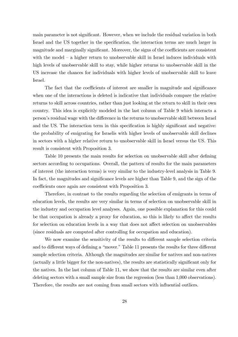
main parameter is not signi…cant. However, when we include the residual variation in both
Israel and the US together in the speci…cation, the interaction terms are much larger in
magnitude and marginally signi…cant. Moreover, the signs of the coe¢cients are consistent
with the model – a higher return to unobservable skill in Israel induces individuals with
high levels of unobservable skill to stay, while higher returns to unobservable skill in the
US increase the chances for individuals with higher levels of unobservable skill to leave
Israel.
The fact that the coe¢cients of interest are smaller in magnitude and signi…cance
when one of the interactions is deleted is indicative that individuals compare the relative
returns to skill across countries, rather than just looking at the return to skill in their own
country. This idea is explicitly modeled in the last column of Table 9 which interacts a
person’s residual wage with the di¤erence in the returns to unobservable skill between Israel
and the US. The interaction term in this speci…cation is highly signi…cant and negative:
the probability of emigrating for Israelis with higher levels of unobservable skill declines
in sectors with a higher relative return to unobservable skill in Israel versus the US. This
result is consistent with Proposition 3.
Table 10 presents the main results for selection on unobservable skill after de…ning
sectors according to occupations. Overall, the pattern of results for the main parameters
of interest (the interaction terms) is very similar to the industry-level analysis in Table 9.
In fact, the magnitudes and signi…cance levels are higher than Table 9, and the sign of the
coe¢cients once again are consistent with Proposition 3.
Therefore, in contrast to the results regarding the selection of emigrants in terms of
education levels, the results are very similar in terms of selection on unobservable skill in
the industry and occupation level analyses. Again, one possible explanation for this could
be that occupation is already a proxy for education, so this is likely to a¤ect the results
for selection on education levels in a way that does not a¤ect selection on unobservables
(since residuals are computed after controlling for occupation and education).
We now examine the sensitivity of the results to di¤erent sample selection criteria
and to di¤erent ways of de…ning a “mover.” Table 11 presents the results for three di¤erent
sample selection criteria. Although the magnitudes are similar for natives and non-natives
(actually a little bigger for the non-natives), the results are statistically signi…cant only for
the natives. In the last column of Table 11, we show that the results are similar even after
deleting sectors with a small sample size from the regression (less than 1,000 observations).
Therefore, the results are not coming from small sectors with in‡uential outliers.
28

Table 12 presents results for di¤erent ways of de…ning a “mover.” The …rst two
columns compare the results obtained using “mover” status as of 2004 to “mover” status
as of 2002. The results are a little weaker and less signi…cant, but are generally similar
using both de…nitions. The third column de…nes a “mover” as someone who is de…ned as
a “mover” in both 2002 and 2004, and the results are still very similar. The last column
de…nes a mover as someone who is categorized as a “mover” in 2004, but also has been
out of the country since the end of 2000. Again, the parameters of interest are signi…cant,
and indicate that the results are robust to con…ning the status of “mover” only to those
who have been out of the country for several years.
6 A Few More Robustness Checks
Tables 13 and 14 present a few more robustness checks for the selection on education
and unobservable skill. The …rst column in Table 13 replicates the benchmark results
used in previous tables. The second column uses the same speci…cations, but uses a
linear probability model (OLS) instead of a probit. The coe¢cient estimates tend to be
considerably stronger and more signi…cant with OLS. The third column estimates the
selection of unobservables, but includes an additional regressor for the interaction between
the di¤erence in residual variation (Israel versus the US) within a person’s sector and the
square of his residual wage. Previous speci…cations only included the interaction with his
residual wage, not his residual wage squared. The coe¢cients on the interaction with the
residual squared are not signi…cant, and the main interaction remains similar in size and
signi…cance. The last column in Table 13 uses an individual’s residual rank within his age
group (30-34, 35-39, and 40-45) instead of his actual residual wage in the analysis, since
the variance of residual wages tends to increase with age. However, the results using ranks
instead of levels are still very similar.
In Table 14, we specify a regression which tests for selection on observable skill (ed-
ucation) and unobservable skill (residual wages) in the same regression. Up to now, we
estimated them separately in di¤erent regressions, since the analysis for observables re-
quired using a …xed-e¤ect for sector only, while the analysis for unobservables requires
a …xed-e¤ect for each sector and education cell. Therefore, it is not appropriate to esti-
mate them together with …xed-e¤ects for cells de…ned by sector or sector-education cells.19
19Using a …xed-e¤ect for each sector and education cell when we test for selection on education meanswe would be testing for selection on education within very small ranges of education, and therefore, webelieve this is not the appropriate speci…cation. Furthermore, including a …xed-e¤ect for sector only in
29

However, despite these concerns, we now estimate the selection on observable and un-
observable skills in the same regression – using …xed-e¤ects for the sector only and then
using …xed-e¤ects for the sector-education cell. Table 13 presents these results for both the
industry and occupation level analysis. Overall, the results are very similar to all of the
previous estimates – a lower relative return to skill increases the level of positive selection
in unobservable skill for both the industry and occupation level analyses, while the results
for observable skill are signi…cant only for the industry level analysis. Essentially, the co-
e¢cient estimates are unchanged from the analysis that estimates each type of selection
separately, and they are robust to whether the …xed-e¤ect is at the sector level or whether
they are de…ned by sector-education cells.
7 The Magnitude of the Coe¢cients
So far, we found statistically signi…cant evidence in favor of increased positive selection on
observable and unobservable skill in sectors with a low relative return to skill in Israel versus
the US. However, the magnitudes of the coe¢cients are not easy to interpret. Therefore, we
now use our estimates to present the relationship between levels of skill and the propensity
to emigrate under alternative scenarios. Speci…cally, we compute the predicted values of
the regression after substituting di¤erent relative returns to skill between Israel and the
US, and show how the relationship between skill and the probability of emigration changes
under each scenario.
For example, Figure 7 compares the actual rates of emigration by education level with
the predicted rates (using the estimated parameters in the last column of Table 5) after
increasing the relative return to education in Israel versus the US by 0.03 (which roughly
makes the average return equal in Israel and the US). Overall, Figure 7 shows that almost
the entire relationship between education and emigration can be eliminated if the relative
returns to skill were similar to those in the US. This simulation suggests that the estimated
selection parameters are not only signi…cant statistically, but are considerably large in
magnitude. (We do not present a similar simulation for the occupation-level analysis
of selection on education, since these coe¢cients were not signi…cant, and therefore, the
magnitudes should be considered close to zero.)
In order to demonstrate the magnitude of selection on unobservable skill, Figure 8
compares the actual emigration rates versus the predicted rates after increasing the residual
the analysis on unobservable skill is not entirely appropriate since the person’s residual wage is interactedwith the return to skill within cells de…ned by sector and education group, not just sector.
30

variation in each sector by 0.025, which is the overall gap in residual variation between the
two countries. Consistent with the model’s predictions, equalizing the residual variance
across the two countries shifts the inverse U-shaped pattern to the left, so that the selection
of emigrants becomes less positive. However, the size of the shift is not noticeably large,
which may be due in part to the small di¤erence in the residual variance between the
two countries as well as the size of the coe¢cient itself. This is seen in Figure 9 which
performs a similar exercise using the coe¢cients from the occupation-level analysis, which
tended to be larger than those in the industry-level analysis on unobservable skills. When
the residual variance is equalized using these estimates, a much larger shift to the left
occurs, thus reducing the positive selection based on unobservable skills in a noticeable
way, while keeping the overall U-shaped pattern intact. Overall, these …gures show that
the parameters governing the selection process on observable and unobservable skills are
signi…cant statistically and also in magnitude.
8 Conclusion
Using a unique data set containing information on the labor market outcomes of individ-
uals before they decide to move or not, this paper presents the most extensive analysis of
emigrant selection based on observable and unobservable skills. Building on the theoretical
framework of Roy (1951) and Borjas (1987, 1991, 1999), we develop a model which predicts
that the relationship between education and emigration should be positive if the relative
return to education is lower in the source country versus a potential host country, while the
relationship between moving and unobservable skills should be characterized by an inverse
U-shaped pattern. The …rst prediction is similar to Borjas (1987), since education is con-
sidered a general skill in our analysis. However, unobservable skills are composed of both
general and country-speci…c skills, and since those at the top of the income distribution are
the most likely to have both types of skill in abundance, they are less likely to risk losing
their country-speci…c skills by moving than those towards the middle of the unobservable
skill distribution. Thus, the pattern for unobservable skills exhibits an inverse U-shape.
These predictions are supported by the general patterns in our data. Furthermore,
we exploit di¤erences across sectors in the relative returns to observable and unobservable
skills between Israel and the United States to identify the causal e¤ect of inequality in
each country on the propensity to emigrate. We …nd strong evidence that a lower return
to unobservable skills in Israel versus the United States entices higher ability Israelis to
31

leave the country. Also, we …nd that the positive relationship between education and the
probability of moving intensi…es in industries with a lower relative return to education
in Israel versus the United States. The estimates suggest that the positive relationship
between education and emigration could be eliminated entirely if the returns to skill were
similar across the two countries.
It is worthwhile to note that these results are unlikely to be due to US immigration
policy. Although US immigration authorities do consider the skill level and sector of work
for each Israeli applying for a visa, the regressions control for sector-speci…c e¤ects (industry
and occupation), and it is highly unlikely that US immigration authorities are running
regressions within each sector in the US and Israel, and tailoring their policies to the relative
returns within each sector between the US and a small country like Israel. Overall, the
results strongly support our model and the importance of di¤erentiating between general
and “country-speci…c” skills in the analysis of immigrant selection.
Our …ndings have important implications regarding the desired level of inequality in
a country. Although the high level of inequality in the United States is commonly regarded
in a negative light, it does play an important role in making the United States a magnet
for the most talented workers in the world. Therefore, to a large degree, a country’s level
of inequality represents how well it will be able to compete with the US for its smartest
people. So, even if a country has a high level of inequality, like Israel, it should be careful
about reducing it in ways that will lead to a signi…cant brain drain.
32

References[1] Akee, Randall. (2010). “Who Leaves? Deciphering Immigrant Self-Selection from a
Developing Country,” Economic Development and Cultural Change, 58 (2), 323-344.
[2] Ben-David, Dan. “Brain Drained: A Tale of Two Countries,” CEPR Working Paper6717, February 2008.
[3] Belot, Michele and Timothy J. Hatton. “Immigrant Selection in the OECD,” CEPRWorking Paper 6675, February 2008.
[4] Borjas, George J. 1987. “Self-Selection and the Earnings of Immigrants.” AmericanEconomic Review 77 (4), September 1987, 531–553.
[5] Borjas, George J. 1991. “Immigration and Self-Selection.” in Immigration, Trade, andthe Labor Market, edited by John M. Abowd and Richard B. Freeman. Chicago:University of Chicago Press (for NBER).
[6] Borjas, George J. 1999. “The Economic Analysis of Immigration.” in Handbook ofLabor Economics, vol.3A, edited by Orley Ashenfelter and David Card. Amsterdam:North-Holland.
[7] Borjas, George J., Stephen G. Bronars, and Stephen J. Trejo. 1992. “Self-Selectionand Internal Migration in the United States.” Journal of Urban Economics 32 (Sep-tember): 159–85.
[8] Brandolini, Andrea and Timothy M. Smeeding. “Inequality: International Evidence,"New Palgrave Dictionary of Economics, forthcoming 2008.
[9] Chiswick, Barry (1999). “Are Immigrants Favorably self-selected?” American Eco-nomic Review – Papers and Proceedings, 89, 2: 181-85.
[10] Chiquiar, Daniel and Gordon Hanson, “International Migration, Self-Selection, andthe Distribution of Wages: Evidence from Mexico and the United States,” Journal ofPolitical Economy, 113(2), 2005, 239-281.
[11] Cobb-Clark, Deborah A. (1993). “Immigrant Selectivity and Wages: The Evidencefor Women,”American Economic Review, 83 (4), September 1993, 986-993.
[12] Dahl, Gordon B. (2002). “Mobility and the Return to Education: Testing a RoyModelwith Multiple Markets,” Econometrica 70 (6), 2367-2420.
[13] Dustmann, Christian and Yoram Weiss (2007). “Return Migration: Theory andEmpirical Evidence from the UK,” British Journal of Industrial Relations 45(2), 236-256.
[14] Dustmann, Christian (2003). “Return migration, wage di¤erentials, and the optimalmigration duration,” European Economic Review 47, 353–369.
[15] Feliciano, C. (2005), “Educational Selectivity in U.S. Immigration: How do Immi-grants Compare to Those Left Behind?” Demography, 42, 131-152.
[16] Friedberg, Rachel M. (2000). “You can’t take it with you? Immigrant assimilationand the portability of human capital,” Journal of Labor Economics, 18 (2): 221–51.
33

[17] Friedberg, Rachel M. (2001). “The Impact of Mass Migration on the Israeli LaborMarket,” Quarterly Journal of Economics, 116 (4), (Nov., 2001), 1373-1408.
[18] Gould, Eric and Omer Moav. “Israel’s Brain Drain,” Israel Economic Review, 5 (1),November 2007, 1-22.
[19] Grogger, Je¤rey and Gordon H. Hanson. (2011) “Income Maximization and the Se-lection and Sorting of International Migrants,” Journal of Development Economics,95 (1), 42-57.
[20] Hamermesh, Daniel S. and Stephen J. Trejo. “How Do Immigrants Spend Time?: TheProcess of Assimilation,” NBER Working Paper 16430, October 2010.
[21] Hanson, Gordon H. (2006). “Illegal Migration from Mexico to the United States,”Journal of Economic Literature, 44 , 869-924.
[22] Hanson, Gordon H. and Antonio Spilimbergo (1999). “Illegal Immigration, BorderEnforcement, and Relative Wages: Evidence from Apprehensions at the U.S.-MexicoBorder,” American Economic Review, Vol. 89 (5), 1337-1357.
[23] Juhn C., K. M. Murphy, and B. Pierce. “Wage Inequality and the Rise in Returns toSkill,” Journal of Political Economy, 101, 1993, 410-442.
[24] McKenzie, David and Hillel Rapoport. (2007). “Self-Selection Patterns in Mexico-U.S.Migration: The Role of Migration Networks.” World Bank Policy Research WorkingPaper 4118.
[25] Mountford, A. (1997), “Can a Brain Drain be Good for Growth in the Source Econ-omy?” Journal of Development Economics, 53, pp. 287-303.
[26] Orrenius, Pia M. and Madeline Zavodny. (2005). “Self-Selection Among Undocu-mented Immigrants From Mexico,” Journal of Development Economics, 78, 2005,215-240.
[27] Roy, Andrew D. (1951), “Some Thoughts on the Distribution of Earnings,” OxfordEconomic Papers, 3 (June 1951), 135-146.
[28] Sjaastad, Larry A. (1962). “The Costs and Returns of Human Migration, Journal ofPolitical Economy, Vol. 70, 5, Part 2: Investment in Human Beings. (October, 1962),80-93.
34

9 APPENDIXWe now present the proofs to the proposition in the main text.
PROOF OF PROPOSITION 1:1. For ¡ 0 if ~ 1 then ~ [0 ~) Since · ~ for ~ · ¡+ ~
1+Ã!
~ · ¡
then ( ~ ) = 0 For ~ 2³¡
1´ as follows from equation (4), ( ~ ) =
~¡¡+ ~1+
~=
1+¡ ¡
(1+) ~ If ~ ¸ 1 then ~ [ ~ ¡ 1 1] For ¡+ ~
1+¸ 1 Ã! ~ ¸
1 + ¡ (¡ ) ( ~ ) = 0 For ~ 2 (1 1 + ¡ (¡ )) as follows from (4), noting
that since 1 and ~ · 2 ¡+ ~1+
~ ¡ 1 ( ~ ) =1¡ ¡+ ~
1+
1¡( ~¡1) = 1+¡(¡)¡ ~(2¡ ~)(1+)
Parts 2-7 follow from the properties of (5). ¤
PROOF OF PROPOSITION 2:The proposition follows directly from the properties of (5), noting that 0 ¤
PROOF OF PROPOSITION 3:For any given ~ and there exists a threshold level of above which individuals
decide to emigrate. In particular, for ~ = 1 it follows that ~ [0 1] and hence thisthreshold level of is represented by (1; ) = 1¡ (1; ) = 1¡ ¡(¡)
+1= 1+(¡)
+1 Since
+ = ~ it follows that an individual at the threshold level of given that ~ = 1 willhave speci…c skills equal to = 1¡ = ¡(¡)
+1 For this individual, by de…nition of being
at the threshold, 0 = 1 and hence + = + Suppose there is a rise in and such that this individual remains indi¤erent, and hence, (1 ) is unchanged. In this case,the rise in is given by = = 1+(¡)
+1 where is the change in
For ~ 2³¡
1´ ( ~ ) =
+1¡ ¡
(1+) ~ Therefore, the change in ( ~ ) ( ~ )
holding (1 ) constant, is
( ~ ) =
µ +
+ + 1¡ + ¡
(1 + + ) ~
¶¡µ
+ 1¡ ¡
(1 + ) ~
¶
Replacing by 1+(¡)+1
,
( ~ ) =
à +
+ + 1¡
+ 1+(¡)+1
¡
(1 + + ) ~
!¡µ
+ 1¡ ¡
(1 + ) ~
¶
and re-arranging:
( ~ ) =1
~
+ 1
~ ¡ 1
+ + 1
Hence, for 0 and ~ 1 ( ~ ) 0
Similarly, for ~ 2 (1 1 + ¡ (¡ )) ( ~ ) = 1+¡(¡)¡ ~(2¡ ~)(1+)
and the change in( ~ ) ( ~ ) holding (1 ) constant is,
( ~ ) =1 + + ¡ (+ ¡ )¡ ~
(2¡ ~) (1 + + )¡ 1 + ¡ (¡ )¡ ~
(2¡ ~) (1 + )
35

replacing by 1+(¡)+1
,
( ~ ) =1 + + ¡
³+ 1+(¡)
+1 ¡
´¡ ~
(2¡ ~) (1 + + )¡ 1 + ¡ (¡ )¡ ~
(2¡ ~) (1 + )
and re-arranging:
( ~ ) =
+ 1
1¡ ~
( ~ ¡ 2) ( + + 1)
Hence, for 0 and ~ 1 ( ~ ) 0 ¤
PROOF OF PROPOSITION 4:First note that the density function derived from the distribution of ~ which is the
sum of two independent uniform distributions on the unit interval, is:
( ~) =
½~ ~ · 1
2¡ ~ ~ 1
Hence, it follows from Proposition 1 that
() =
2Z
0
( ~ ) ( ~) ~
=
1Z
¡
µ
+ 1¡ ¡
(1 + ) ~
¶( ~) ~ +
1+¡(¡)Z
1
µ1 + ¡ (¡ )¡ ~
(2¡ ~) (1 + )
¶( ~) ~
=1
2 ( + 1)( ¡ + )2 +
1
2 ( + 1)( ¡ + )2
= ( ¡ + )2
µ1
2 ( + 1)+
1
2 ( + 1)
¶
=( ¡ + )2
2
the derivatives appearing in the proposition are straightforward noting that
36

Appendix Figures
The following simulations were conducted by assuming that the unobservable general
and country-specific skills, g and s, are normally distributed with different specifications
for the correlation between them. For both g and s, we assume a mean of 1 and a
standard deviation of 1. Values of g and s are truncated to be positive, since negative
values of s would create an incentive in our model to leave Israel just to get rid of their
country-specific skills. The simulations are conducted with a=0.1 (the total fixed cost of
moving) and γ=0.1 (the difference in the return to g between the host and the home
country), and we abstract from schooling by assuming that years of education equal zero.
The first figure shows that an inverse U-shaped pattern between the probability of
emigrating and residual wages is also obtained after simulating the model with a normal
distribution for both of the unobservable skills (instead of the uniform distribution used in
the main text). The second and third figures show a similar pattern even if we allow for a
negative or positive correlation between the two skills (still assumed to be normal).
0
.005
.01
.015
.02
.025
Fra
ction
Lea
vin
g Isra
el
1 2 3 4 5 6 7 8 9 10Simulated Residual Wage Decile
G and S are Normal with a Correlation = 0
Appendix Figure 1: Simulation using the Normal Distribution

1
-.0
05
0
.005
.01
.015
Fra
ction
Lea
vin
g Isra
el
1 2 3 4 5 6 7 8 9 10Simulated Residual Wage Decile
G and S are Normal with a Correlation = 0.3
Appendix Figure 2: Simulation using the Normal Distribution
0
.01
.02
.03
Fra
ction
Lea
vin
g Isra
el
1 2 3 4 5 6 7 8 9 10Simulated Residual Wage Decile
G and S are Normal with a Correlation = -0.3
Appendix Figure 3: Simulation using the Normal Distribution

2
Table 1: Descriptive Statistics for Male Workers from the 1995 Israel Census
Mean
Standard Deviation
Mover 2004 0.016 0.126
Mover 2002 0.013 0.114
Returned 2002-2004 (for Movers 2002) 0.020 0.141
Left by end of 2000 (for Movers 2004) 0.672 0.470
Education 13.011 3.187
Age 37.773 4.613
Married 0.898 0.303
Native 0.614 0.487
Age Arrived in Israel (non-natives only) 20.344 13.274
Asia-Africa Origin 0.466 0.499
European Origin 0.480 0.500
Israeli Origin 0.054 0.227
Number of Children 2.130 1.366
Log Wage (monthly) 8.605 0.593
Observations 40713
The core sample used throughout the paper and in this table includes all male respondents between the ages
of 30 and 45 in the 1995 Israel Census who were not self-employed, worked at least 30 hours a week, and
worked at least six months in the previous 12 months. Wages are monthly wages in Israeli Shekels using
1995 prices.

3
Table 2: Descriptive OLS Regressions for Male Workers in Israel and the US
Log Wage
Mover
(from Israel)
2004
Returned
(to Israel)
2002-2004
US
(CPS Data)
Israel
(1995
Census)
Education 0.100*** 0.071*** 0.002*** -0.002
(0.001) (0.001) (0.000) (0.002)
Age 0.108*** 0.080*** -0.003 0.002
(0.012) (0.010) (0.002) (0.025)
Age-squared -0.001*** -0.001*** 0.000 -0.000
(0.000) (0.000) (0.000) (0.000)
Married 0.223*** 0.186*** -0.003 -0.009
(0.006) (0.008) (0.002) (0.019)
Year 1994 -0.008
(0.007)
Year 1996 0.002
(0.007)
Native -0.099*** 0.005*** -0.016
(0.008) (0.002) (0.026)
Age Arrived in
Israel -0.019*** 0.001*** -0.001
(0.000) (0.000) (0.001)
Asia-Africa
Origin -0.161 -0.000 0.005
(0.011) (0.003) (0.034)
European Origin -0.016 0.001 0.039
(0.012) (0.003) (0.033)
Log Wage -0.001 0.003
(0.003) (0.014)
Intercept 5.271*** 5.921*** 0.070 -0.024
(0.214) (0.184) (0.047) (0.459)
Root MSE 0.523 0.498
Observations 33,302 40,713 40,713 538 * indicates significance at the 10% level, ** at the 5% level, and *** at the 1% level. The Israel sample is
described in Table 1. The sample for the United States comes from the 1994, 1995, and 1996 March CPS
files (dummy variables are included in the specifications for each sample year). The US sample includes
all white, native, male respondents between the ages of 30 and 45 in the three CPS files who were not self-
employed, worked at least 30 hours a week, and worked at least six months in the previous 12 months.
Wages are monthly wages and are adjusted to 1995 price levels using the CPI-U index.

4
Table 3: Industry Descriptive Statistics of the Israeli Sample with US CPS Variables
N
Mean
Mover
2004
Mean
Log
Wage
Mean
Educa-
tion
ROR to
Educ in
Israel
ROR to
Educ in
US
Residual
SD in
Israel
Residual
SD in
US
Agriculture,
Forestry,
Fishing
663 0.015 8.199 11.157 0.039 0.070 0.488 0.525
Mfg
13493 0.017 8.561 12.723 0.078 0.113 0.451 0.500
Electric, Water 1038 0.014 8.821 13.163 0.058 0.079 0.418 0.407
Construction
2939 0.020 8.463 11.939 0.064 0.091 0.479 0.543
Wholesale and
Retail
6270 0.014 8.533 12.341 0.072 0.094 0.513 0.535
Trans., Storage,
Comm.
3331 0.011 8.610 12.036 0.072 0.088 0.510 0.531
Bank, Finance,
Insurance
1627 0.010 8.996 14.286 0.068 0.108 0.467 0.496
Real Estate,
Business
3776 0.022 8.784 14.871 0.069 0.124 0.533 0.535
Public Admin.
3216 0.008 8.685 12.801 0.067 0.067 0.417 0.439
Education
1488 0.018 8.578 15.545 0.052 0.073 0.484 0.440
Health,
Welfare, Social
Work
1693 0.028 8.674 15.282 0.073 0.122 0.605 0.543
Social Service
1179 0.015 8.467 12.602 0.061 0.066 0.531 0.567
Industry categories were matched across the Israeli 1995 Census and the CPS files from the US. The rate of
return to education in each sector in Israel comes from a regression specified in the second column of Table 2,
but run on a sample of workers within each sector. The “Residual SD” for each sector in Israel comes from the
same set of regressions and is computed by calculating the standard deviation of residuals within each education
group (high school dropouts, high school graduates, and college graduates) within each sector, and then
computing the mean by sector. Similarly, the returns to education and “Residual SD” for the US comes from
similar regressions as specified in the first column in Table 1 for each sector.

5
Table 4: Occupation Descriptive Statistics of the Israeli Sample with US CPS Variables
N
Mean
Mover
2004
Mean
Log
Wage
Mean
Educa-
tion
ROR to
Educ in
Israel
ROR to
Educ in
US
Residual
SD in
Israel
Residual
SD in US
Academic
Professionals 5624 0.027 8.945 16.842 0.016 0.067 0.516 0.489
Associate
Professionals
and
Technicians
3867 0.018 8.723 14.044 0.041 0.070 0.467 0.475
Managers
4452 0.012 9.139 14.371 0.047 0.098 0.511 0.507
Clerical
4395 0.008 8.610 12.764 0.063 0.054 0.452 0.521
Agents, Sales,
and Service
4429 0.012 8.496 12.183 0.054 0.113 0.489 0.571
Skilled
Agricultural
516 0.016 8.152 11.258 0.036 0.060 0.462 0.529
Skilled
Workers
13835 0.017 8.379 11.472 0.045 0.070 0.438 0.509
Unskilled
Workers
3595 0.014 8.348 11.717 0.063 0.054 0.473 0.532
Occupation categories were matched across the Israeli 1995 Census and the CPS files from the US. The
rate of return to education in each sector in Israel comes from a regression specified in the second column
of Table 2, but run on a sample of workers within each sector. The “Residual SD” for each sector in Israel
comes from the same set of regressions and is computed by calculating the standard deviation of residuals
within each education group (high school dropouts, high school graduates, and college graduates) within
each sector, and then computing the mean by sector. Similarly, the returns to education and “Residual SD”
for the US comes from similar regressions as specified in the first column in Table 1 for each sector.

6
Table 5: Selection on Education – Main Results for the Industry Level Analysis
Probit for being a Mover in 2004
Education* -0.0146 -0.0930***
Israel ROR Educ in Industry i (0.018) (0.027)
Education*
0.0202** 0.0511***
US ROR Educ in Industry i (0.0083) (0.012)
Education* -0.0427***
Diff between Israel and US in (0.011)
ROR Educ in Industry i
Industry Wage Residual 0.000155 0.000144 0.000119 0.000130
(0.0010) (0.0010) (0.0010) (0.0010)
Industry Wage Residual2 -0.00481*** -0.00481*** -0.00482*** -0.00482***
(0.0015) (0.0015) (0.0015) (0.0015)
Education 0.00217* -0.000903 0.00254* -0.000170
(0.0013) (0.00085) (0.0014) (0.00038)
Married 0.00132 0.00128 0.00126 0.00126
(0.0014) (0.0014) (0.0014) (0.0014)
Number of Children -0.00199*** -0.00199*** -0.00201*** -0.00200***
(0.00045) (0.00045) (0.00045) (0.00045)
Native 0.00249 0.00244 0.00242 0.00242
(0.0017) (0.0017) (0.0017) (0.0017)
Age Arrived in Israel 0.000634*** 0.00063*** 0.000631*** 0.000632***
(0.000062) (0.00006) (0.000061) (0.000061)
Industry Fixed Effects Yes Yes Yes Yes
Observations 40,713 40,713 40,713 40,713 * indicates significance at the 10% level, ** at the 5% level, and *** at the 1% level. All specifications
include controls for age, age-squared, and ethnic dummies.. Coefficients are the marginal effects calculated
at the sample means of the explanatory variables.

7
Table 6: Selection on Education – Main Results for the Occupation Level Analysis
Probit for being a Mover in 2004
Education* -0.0297** -0.0298**
Israel ROR Educ in Occup i (0.012) (0.012)
Education*
-0.0221** -0.0219**
US ROR Educ in Occup i (0.010) (0.0099)
Education* 0.00157
Diff between Israel and US in (0.0079)
ROR Educ in Occupation i
Occupation Wage Residual -0.000909 -0.000868 -0.000871 -0.000895
(0.0011) (0.0011) (0.0011) (0.0011)
Occupation Wage Residual2 -0.00482*** -0.00480*** -0.00484*** -0.00478***
(0.0015) (0.0015) (0.0015) (0.0015)
Education 0.00240*** 0.00269*** 0.00400*** 0.00113***
(0.00058) (0.00075) (0.00093) (0.00029)
Married 0.00115 0.00110 0.00117 0.00109
(0.0014) (0.0014) (0.0014) (0.0015)
Number of Children -0.00200*** -0.00197*** -0.00201*** -0.00196***
(0.00045) (0.00045) (0.00045) (0.00045)
Native 0.00262 0.00255 0.00262 0.00255
(0.0017) (0.0017) (0.0017) (0.0017)
Age Arrived in Israel 0.000646***
0.000635**
* 0.000644*** 0.000637***
(0.000062) (0.000062) (0.000062) (0.000062)
Occupation Fixed Effects Yes Yes Yes Yes
Observations 40,713 40,713 40,713 40,713 * indicates significance at the 10% level, ** at the 5% level, and *** at the 1% level. All specifications
include controls for age, age-squared, and ethnic dummies.. Coefficients are the marginal effects calculated
at the sample means of the explanatory variables.

8
Table 7: Selection on Education – Sensitivity to Sample Selection
Probit for being a Mover in 2004
Industry Level Analysis
Education* -0.0427*** -0.0484*** -0.0321 -0.0426***
Diff between Israel and US
in ROR Educ in Industry i
(0.011) (0.012) (0.024) (0.011)
Sample Restriction None Natives Non-Natives Industries
with Sample
Size > 1000
Industry Fixed Effects Yes Yes Yes Yes
Observations 40,713 25,011 15,702 40,050
Occupation Level Analysis
Education* 0.00157 0.00509 -0.00612 0.00147
Diff between Israel and US
in ROR Educ in Occupation i
(0.0079) (0.0096) (0.016) (0.0079)
Sample Restriction None Natives Non-Natives Occupations
with Sample
Size > 1000
Occupation Fixed Effects Yes Yes Yes Yes
Observations 40,713 25,011 15,702 40,197 * indicates significance at the 10% level, ** at the 5% level, and *** at the 1% level. All specifications
include controls for education, age, age-squared, ethnic dummies, marital status, native status, and age
arrived in Israel (if non-native). The industry analysis also controls for the individual’s residual wage
within his industry and its square, while the occupation analysis controls for the individual’s residual wage
within his occupation and its square. Coefficients are the marginal effects calculated at the sample means of
the explanatory variables.

9
Table 8: Selection on Education – Sensitivity to Various Definitions of a “Mover”
Mover 2004
Mover
2002
Mover 2002
and 2004
Mover 2004
since 2000
Industry Level Analysis
Education* -0.0427*** -0.0321*** -0.0315*** -0.0269***
Diff between Israel and US in (0.011) (0.010) (0.010) (0.0090)
ROR Educ in Industry i
Industry Fixed Effects Yes Yes Yes Yes Observations 40,713 40,713 40,713 40,713
Occupation Level Analysis
Education* 0.00157 0.00136 0.00151 -0.00103
Diff between Israel and US in (0.0079) (0.0074) (0.0073) (0.0064)
ROR Educ in Occupation i Occupation Fixed Effects Yes Yes Yes Yes
Observations 40,713 40,713 40,713 40,713 * indicates significance at the 10% level, ** at the 5% level, and *** at the 1% level. All specifications
include controls for education, age, age-squared, ethnic dummies, marital status, native status, and age
arrived in Israel (if non-native). The industry analysis also controls for the individual’s residual wage
within his industry and its square, while the occupation analysis controls for the individual’s residual wage
within his occupation and its square. Coefficients are the marginal effects calculated at the sample means of
the explanatory variables.

10
Table 9: Selection on Unobservables – Main Industry Level Analysis
Probit for being a Mover in 2004
Industry Wage Residual* -0.0212 -0.0295*
Israel Residual SD (0.015) (0.016)
in Industry-Education Group i
Industry Wage Residual*
0.0219 0.0357
US Residual SD (0.021) (0.022)
in Industry-Education Group i
Industry Wage Residual * -0.0311**
Difference between Israel and (0.015)
US in Residual SD
in Industry-Education Group i
Industry Wage Residual 0.0106 -0.0113 -0.00328 -0.000146
(0.0077) (0.011) (0.012) (0.0010)
Industry Wage Residual2 -0.00524*** -0.00494*** -0.00549*** -0.00550***
(0.0015) (0.0015) (0.0015) (0.0015)
Education 0.000862*** 0.00085*** 0.000864*** 0.000865***
(0.00025) (0.0003) (0.00025) (0.00025)
Married 0.00114 0.00113 0.00112 0.00113
(0.0014) (0.0014) (0.0014) (0.0014)
Number of Children -0.00191*** -0.00191*** -0.00190*** -0.00190***
(0.00045) (0.00045) (0.00045) (0.00045)
Native 0.00218 0.00215 0.00213 0.00214
(0.0017) (0.0017) (0.0017) (0.0017)
Age Arrived in Israel 0.000609*** 0.00061*** 0.000606*** 0.000606***
(0.000062) (0.00006) (0.000062) (0.000062)
Industry-Education Group Yes Yes Yes Yes
Fixed Effects
Observations 40,412 40,412 40,412 40,412 * indicates significance at the 10% level, ** at the 5% level, and *** at the 1% level. All specifications
include controls for age, age-squared, and ethnic dummies.. Coefficients are the marginal effects calculated
at the sample means of the explanatory variables.

11
Table 10: Selection on Unobservables – Main Occupation Level Analysis
Probit for being a Mover in 2004
Occupation Wage Residual* -0.0764*** -0.0785***
Israel Residual SD (0.028) (0.028)
in Occup-Education Group i
Occupation Wage Residual*
0.0245 0.0303
US Residual SD (0.029) (0.029)
in Occup-Education Group i
Occupation Wage Residual *
-0.0552***
Difference between Israel and (0.021)
US in Residual SD
in Occup-Education Group i
Occupation Wage Residual 0.0357*** -0.0135 0.0213 -0.00257**
(0.014) (0.015) (0.019) (0.0012)
Occupation Wage Residual2 -0.00569*** -0.00493*** -0.00584*** -0.00569***
(0.0015) (0.0015) (0.0015) (0.0015)
Education 0.000897*** 0.00088*** 0.000896*** 0.000892***
(0.00024) (0.0003) (0.00024) (0.00024)
Married 0.000969 0.000999 0.000956 0.000958
(0.0014) (0.0014) (0.0014) (0.0014)
Number of Children -0.00187*** -0.00190*** -0.00186*** -0.00187***
(0.00044) (0.00044) (0.00044) (0.00044)
Native 0.00224 0.00225 0.00222 0.00221
(0.0017) (0.0017) (0.0017) (0.0017)
Age Arrived in Israel 0.000596*** 0.00060*** 0.000596*** 0.000596***
(0.000063) (0.00006) (0.000063) (0.000063)
Occupation-Education Group Yes Yes Yes Yes
Fixed Effects
Observations 40,621 40,621 40,621 40,621 * indicates significance at the 10% level, ** at the 5% level, and *** at the 1% level. All specifications
include controls for age, age-squared, and ethnic dummies.. Coefficients are the marginal effects calculated
at the sample means of the explanatory variables.

12
Table 11: Selection on Unobservables – Sensitivity to Sample Selection
Probit for being a Mover in 2004
Industry Level Analysis
Industry Wage Residual * -0.0311** -0.0244* -0.0340 -0.0331**
Difference between Israel (0.015) (0.014) (0.033) (0.015)
and US in Residual SD in
Industry-Education Group i
Sample Restriction None Natives Non-Natives Industries
with Sample
Size > 1000
Industry-Education Group Yes Yes Yes Yes
Fixed Effects
Observations 40,412 24,674 15,602 39,749
Occupation Level Analysis
Occupation Wage Residual * -0.0552*** -0.0515** -0.0636 -0.0621***
Difference between Israel (0.021) (0.023) (0.044) (0.021)
and US in Residual SD in
Occup-Education Group i
Sample Restriction None Natives Non-Natives Occupations
with Sample
Size > 1000
Occupation-Education Group Yes Yes Yes Yes
Fixed Effects
Observations 40,621 24,573 15,673 40,105
* indicates significance at the 10% level, ** at the 5% level, and *** at the 1% level. All specifications
include controls for education, age, age-squared, ethnic dummies, marital status, native status, and age
arrived in Israel (if non-native). The industry analysis also controls for the individual’s residual wage
within his industry and its square, while the occupation analysis controls for the individual’s residual wage
within his occupation and its square. Coefficients are the marginal effects calculated at the sample means of
the explanatory variables.

13
Table 12: Selection on Unobservables – Sensitivity to Definitions of a “Mover”
Mover 2004
Mover
2002
Mover 2002
and 2004
Mover 2004
since 2000
Industry Level Analysis
Industry Wage Residual * -0.0311** -0.0223 -0.0236* -0.0226*
Difference between Israel (0.015) (0.014) (0.014) (0.012)
and US in Residual SD in
Industry-Education Group i
Industry-Education Group Yes Yes Yes Yes
Fixed Effects
Observations 40,412 40,412 40,412 40,412
Occupation Level Analysis
Occupation Wage Residual * -0.0552*** -0.0449** -0.0442** -0.0406**
Difference between Israel (0.021) (0.019) (0.019) (0.017)
and US in Residual SD in
Occup-Education Group i
Occupation-Education Group Yes Yes Yes Yes
Fixed Effects
Observations 40,621 40,621 40,621 40,621
* indicates significance at the 10% level, ** at the 5% level, and *** at the 1% level. All specifications
include controls for education, age, age-squared, ethnic dummies, marital status, native status, and age
arrived in Israel (if non-native). The industry analysis also controls for the individual’s residual wage
within his industry and its square, while the occupation analysis controls for the individual’s residual wage
within his occupation and its square. Coefficients are the marginal effects calculated at the sample means of
the explanatory variables.

14
Table 13: Various Robustness Checks for Mover 2004 Status
Industry Level Analysis Education* -0.0427*** -0.0610*** -0.0422***
Diff between Israel and US in (0.011) (0.015) (0.011)
ROR Educ in Industry i
Industry Wage Residual
(or Residual Rank) * -0.0311** -0.0348* -0.0291* -0.00422*
Difference between Israel (0.015) (0.020) (0.015) (0.0025)
and US in Residual SD
Industry Wage Residual Squared* 0.00814
Difference between Israel (0.018)
and US in Residual SD
Occupation Level Analysis
Education* 0.00157 -0.00429 0.00209
Diff between Israel and US in (0.0079) (0.010) (0.0079)
ROR Educ in Occupation i
Occupation Wage Residual
(or Residual Rank) * -0.0552*** -0.0677*** -0.0528** -0.00727**
Difference between Israel (0.021) (0.026) (0.021) (0.0032)
and US in Residual SD
Occup Wage Residual Squared* 0.0298
Difference between Israel (0.029)
and US in Residual SD
Using Residual Ranks within
each 5-year Age Group
No No No Yes
Probit or OLS Probit OLS Probit Probit
* indicates significance at the 10% level, ** at the 5% level, and *** at the 1% level. Within each panel,
each column represents a separate regression. The first column represents the “benchmark” specifications
described in earlier tables. Changes to the benchmark specifications are described according to the
information provided in the table. Residual ranks were computed within the individual’s age group, where
the age groups are 30-34, 35-39, and 40-45. Coefficients represent the marginal effects (calculated at the
sample means of the explanatory variables if it comes from a probit).

15
Table 14: Estimating Selection on Education and Unobservables Together
Probit for being a Mover in 2004
Industry Analysis
Occupation Analysis
Education* -0.0418*** -0.0306*
Diff between Israel and US in (0.011) (0.017)
ROR Educ in Industry i
Industry Wage Residual * -0.0308** -0.0303**
Difference between Israel (0.015) (0.015)
and US in Residual SD in
Industry-Education Group i
Education* 0.00184 -0.0123
Diff between Israel and US in (0.0078) (0.011)
ROR Educ in Occupation i
Occupation Wage Residual *
-0.0568*** -0.0546***
Difference between Israel (0.021) (0.021)
and US in Residual SD in
Occup-Education Group i
Industry Fixed Effects
Yes
No
Industry-Education Group
No
Yes
Fixed Effects
Occupation Fixed Effects Yes No
Occupation-Education Group
No
Yes
Fixed Effects
Observations 40,713 40,412 40,713 40,621 * indicates significance at the 10% level, ** at the 5% level, and *** at the 1% level. All specifications
include controls for education, age, age-squared, ethnic dummies, marital status, native status, and age
arrived in Israel (if non-native). The industry analysis also controls for the individual’s residual wage
within his industry and its square, while the occupation analysis controls for the individual’s residual wage
within his occupation and its square. Coefficients are the marginal effects calculated at the sample means of
the explanatory variables.

16
.006562.007169
.009029
.0259150
.005
.01
.015
.02
.025
Fra
ction
Lea
vin
g Isra
el
HS Dropouts HS Graduates BA Degree MA Degree or More
30 to 45 Year Old Israelis
Figure 1a: Native Israelis Leaving Israel By Education
.01313
.021701
.030564
.056843
0
.02
.04
.06
Fra
ction
Lea
vin
g Isra
el
HS Dropouts HS Graduates BA Degree MA Degree or More
30 to 45 Year Old Israelis
Figure 1b: Non-Native Israelis Leaving Israel By Education

17
.025104 .025122
.0306170
.01
.02
.03
Fra
ction
Lea
vin
g Isra
el
HS Dropouts HS Graduates HS Graduates +
22 to 29 Year Old Israeli Males
Figure 2a: Israelis Leaving Israel By Education Level
.022278
.027367
.031523
.037037
0
.01
.02
.03
.04
Fra
ction
Lea
vin
g Isra
el
HS Dropouts HS Graduates BA Degree MA Degree or More
13 to 17 Year Old Israelis
Figure 2b: Israelis Leaving Israel By Father's Education
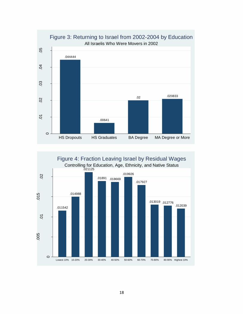
18
.044444
.00641
.02 .020833
0
.01
.02
.03
.04
.05
Fra
ction
Lea
vin
g Isra
el
HS Dropouts HS Graduates BA Degree MA Degree or More
All Israelis Who Were Movers in 2002
Figure 3: Returning to Israel from 2002-2004 by Education
.011542
.014988
.021125
.01891 .018669
.019926
.017927
.013019 .012776.012039
0
.005
.01
.015
.02
Fra
ction
Lea
vin
g Isra
el
Lowest 10% 10-20% 20-30% 30-40% 40-50% 50-60% 60-70% 70-80% 80-90% Highest 10%
Controlling for Education, Age, Ethnicity, and Native Status
Figure 4: Fraction Leaving Israel by Residual Wages

19
.010806
.017199
.020874
.016704
.018423.019165
.017191
.014738
.013514
.012282
0
.005
.01
.015
.02
Fra
ction
Lea
vin
g Isra
el
Lowest 10% 10-20% 20-30% 30-40% 40-50% 50-60% 60-70% 70-80% 80-90% Highest 10%
Controlling for Industry, Education, Age, Ethnicity, and Native Status
Figure 5: Fraction Leaving Israel by Residual Wages
.01203
.015733
.019406
.017436
.020388 .020147
.017927
.013261.014008
.010565
0
.005
.01
.015
.02
Fra
ction
Lea
vin
g Isra
el
Lowest 10% 10-20% 20-30% 30-40% 40-50% 50-60% 60-70% 70-80% 80-90% Highest 10%
Controlling for Occupation, Education, Age, Ethnicity, and Native Status
Figure 6: Fraction Leaving Israel by Residual Wages
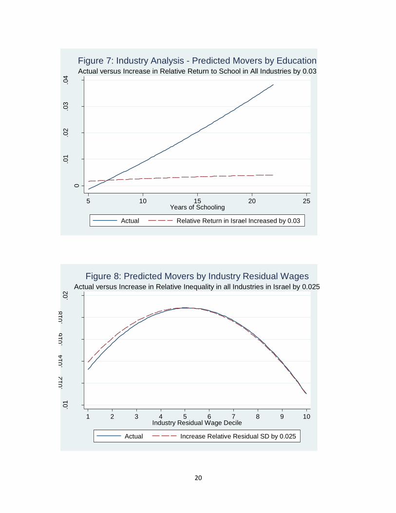
20
0
.01
.02
.03
.04
Fra
ctio
n L
eavin
g Isra
el
5 10 15 20 25Years of Schooling
Actual Relative Return in Israel Increased by 0.03
Actual versus Increase in Relative Return to School in All Industries by 0.03
Figure 7: Industry Analysis - Predicted Movers by Education
.01
.01
2.0
14
.01
6.0
18
.02
Fra
ctio
n L
eavin
g Isra
el
1 2 3 4 5 6 7 8 9 10Industry Residual Wage Decile
Actual Increase Relative Residual SD by 0.025
Actual versus Increase in Relative Inequality in all Industries in Israel by 0.025
Figure 8: Predicted Movers by Industry Residual Wages

21
.0
1.0
12
.01
4.0
16
.01
8.0
2
Fra
ctio
n L
eavin
g Isra
el
1 2 3 4 5 6 7 8 9 10Occupation Residual Wage Decile
Actual Increase Relative Residual SD by 0.025
Actual versus Increase in Relative Inequality in all Occupations in Israel by 0.025
Figure 9: Predicted Movers by Occupation Residual Wages


