Gould Belt Philippe André CEA Far Laboratoire AIM...
17
Highlights from the Herschel Gould Belt survey: Toward a Unified Picture for Star Formation on GMC scales ? Philippe André CEA Laboratoire AIM Paris-Saclay PACS Near Far Herschel Gould Belt Survey Aquila GOODS-N HERMES SAG 3 The Universe Explored by Herschel – ESTEC – 15 Oct 2013
Transcript of Gould Belt Philippe André CEA Far Laboratoire AIM...

Highlights from the Herschel Gould Belt survey:!
Toward a Unified Picture for Star Formation on GMC scales ? !
Philippe André!CEA!
Laboratoire AIM Paris-Saclay!
PACS
Near
Far
Herschel Gould Belt Survey
Aquila
GOODS-N HERMES
SAG 3!
The Universe Explored by Herschel – ESTEC – 15 Oct 2013
Herschel !GB survey!IC5146!Arzoumanian!et al. 2011!
Outline:!
• « Universality » of the filamentary structure of the ISM!
• The key role of filaments in the star formation process!
• Implications and future prospects!
With: D. Arzoumanian, V. Könyves, P. Palmeirim, A. Menshchikov, N. Schneider, A. Roy, N. Peretto, P. Didelon, J. Di Francesco, S. Bontemps, F. Motte, D. Ward-Thompson, J. Kirk, M. Griffin, S. Pezzuto, S. Molinari, M. Benedettini, V. Minier, B. Merin, N. Cox, T. Henning & ! ! the Herschel Gould Belt KP Consortium (inc. SPIRE SAG 3) !
Ph. André – The Universe Explored by Herschel– 15/10/2013
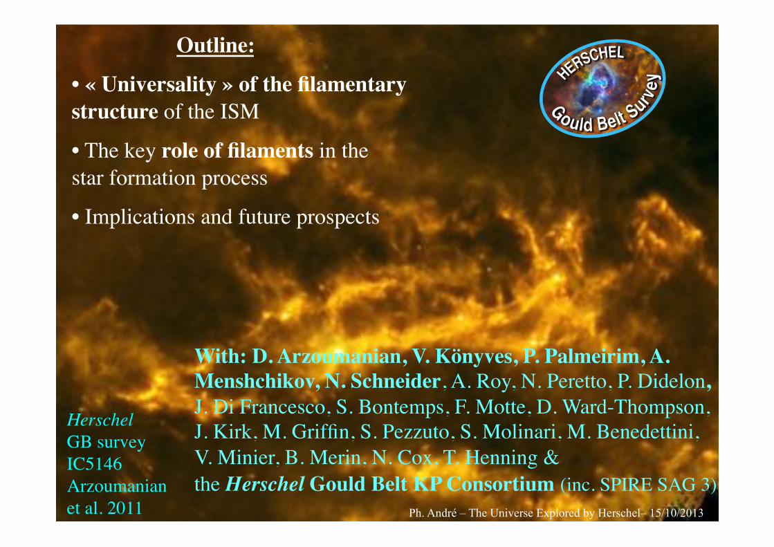
~ 5 pc
Filamentary structure of the cold ISM prior to SF
~ 13 deg2 field
Polaris flare translucent cloud
(d ~ 150 pc) ~ 5500 M� (CO+HI) Heithausen & Thaddeus ‘90
Miville-Deschênes et al. 2010 Ward-Thompson et al. 2010 Men’shchikov et al. 2010 André et al. 2010 A&A vol. 518 SPIRE 250 µm image
Gould Belt Survey Herschel // mode 70/160/250/350/500 µm
Ph. André – The Universe Explored by Herschel– 15/10/2013
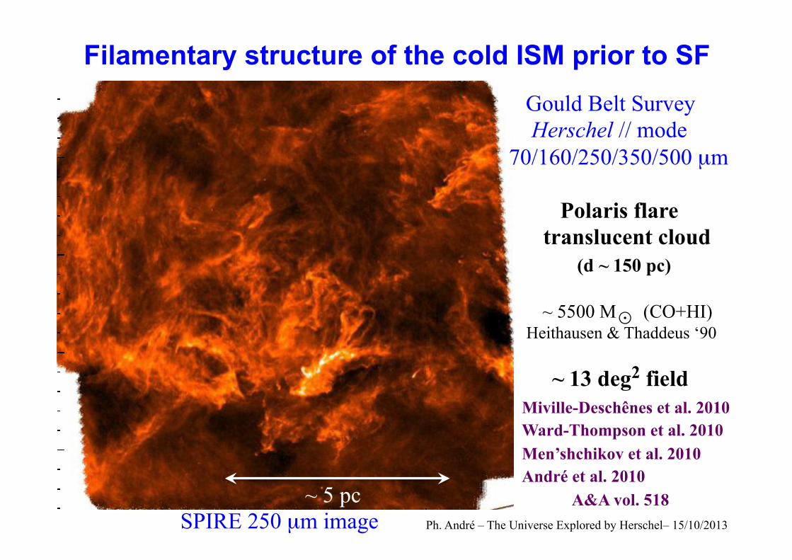
Evidence of the importance of filaments prior to Herschel but … much fainter filaments + universality with Herschel
See also: Schneider & Elmegreen 1979; Abergel et al. 1994; Johnstone & Bally 1999; Hatchell et al. 2005; Goldsmith et al. 2008; Myers 2009 … + Many numerical simulations
966 L. Cambresy: Mapping of the extinction using star counts
Fig. 1. Extinction map of Vela from B counts (J2000 coordinates)
Fig. 2. Extinction map of Carina from R counts (J2000 coordinates)
an adaptive grid where the number of stars in each cell remains
constant. Practically, I used a fixed number of 20 stars per cell
and a filtering method involving a wavelet decomposition that
filters the noise. This method has been described in more details
by Cambresy (1998).
I have applied the method to 24 GMCs. Counts and filtering
are fully automatic. Because of the wide field (� 250 squaredegrees for Orion), the counts must be corrected for the vari-
Fig. 3. Extinction map of Musca from R counts (J2000 coordinates)
ation of the background stellar density with galactic latitude.
Extinction and stellar density are related by:
A� =1a
log�
Dref (b)D
⇥
(1)
where A� is the extinction at the wavelength �, D is the back-
ground stellar density, Dref the density in the reference field
(depending on the galactic latitude b), and a is defined by:
a =log(Dref ) ⇤ cst.
m�(2)
wherem� is the magnitude at the wavelength �.Assuming an exponential law for the stellar density,
Dref (b) = D0 e⇥⇥|b|, a linear correction with the galac-tic latitude b must be applied to the extinction value givenby Eq. (1). The correction consists, therefore, in subtracting
log[Dref (b)] = log(D0) ⇤ ⇥|b| log (e) to the extinction valueA�(b). This operation corrects the slope of A�(b) which be-comes close to zero, and set the zero point of extinction. All
maps are converted into visual magnitudes assuming an extinc-
tion law of Cardelli et al. (1989) for which ABAV
= 1.337 andARAV
= 0.751.Here, the USNO-PMM catalogue (Monet, 1996) is used to
derive the extinction map. It results from the digitisation of
POSS (down to ⇤35� in declination) and ESO plates (⇤ ⇥⇤35�) in blue and red. Internal photometry estimators are be-lieved to be accurate to about 0.15 magnitude but systematic
errors can reach 0.25 magnitude in the North and 0.5 magni-
tude in the South. Astrometric error is typically of the order
of 0.25 arcsecond. This accuracy is an important parameter in
order to count only once those stars which are detected twice
because they are located in the overlap of two adjacent plates.
Cox et al.: Far-infrared observations of the Musca dark cloud, Online Material p 1
Polarisation vectors (Pereyra & Magelhaes, 2004)
Fig. 11. Polarisation vectors for field stars in Musca region (Pereyra & Magelhaes 2004). Colour version is available in the electronic version.
500mu160mu 350mu250mu
Fig. 12. The footprints of the sources extracted with getsources in the Musca region for the maps at 160, 250, 350, and 500µm. Colour version isavailable in the electronic version.
Table 6. Bright extended sources with log(F250/F350) < 0.0, located near or in the main filament. Marked with green ellipses in Fig. 7.
Ra Dec F250 F350 F500 log(F250/F350) major axis minor axis(!) (!) (Jy) (Jy) (Jy) ("") ("")
188.28 -71.08 4.05 6.04 5.81 -0.17 111.9 59.9186.70 -71.49 51.57 68.44 36.52 -0.12 271.8 145185.26 -72.49 4.30 5.65 1.92 -0.12 108.8 50.0185.87 -71.95 2.65 3.36 2.78 -0.10 96.5 42.2186.46 -71.56 2.94 3.61 1.88 -0.09 106.4 48.1
Cambrésy 1999
Extinction map of Musca
Polarization vectors overlaid on Herschel image of Musca
N. Cox et al. + Pereyra & Magelhaes 2004
B field
Musca
N. Cox et al., in prep. - See Poster B-37
Herschel 250 µm
Ph. André – The Universe Explored by Herschel– 15/10/2013

Taurus B211/3 filament: M/L ~ 50 M�/pc
Very common pattern: main filament + network of perpendicular striations or “sub-filaments”
P. Palmeirim et al. 2013
SPIRE 250µm
M. Hennemann et al.: The spine of the swan
Fig. 1. Herschel maps of the DR21 environment a) at 70 µm, b) in column density, and c) in dust temperature (24⇧⇧ angular resolution). The DR21filament is delimited roughly by the NH2 = 1023 cm�2 contour plotted in panels b) and c). The subfilaments studied in Section 3 are marked withdots along their crests in b) and c).
2. Observations and data reduction
Cygnus X North was observed in the Herschel parallel scan mapmode with PACS and SPIRE on Dec 18, 2010 (ObservationalDay 584). To diminish scanning artifacts, two nearly perpen-dicular coverages of 2.8⇥2.8⇤ were obtained in five photomet-ric bands at 70, 160, 250, 350, and 500 µm with a scan speedof 20”/sec. The SPIRE data were reduced using the HerschelInteractive Processing Environment (HIPE, version 7), and forPACS also the Scanamorphos software (Roussel 2012, version12). The 70 µm map (Fig. 1) shows a wealth of structure and inparticular traces heated dust e.g. towards DR21 itself. To quanti-tatively estimate the distribution of the cold dust which generallyrepresents most of the dust mass, we created maps of columndensity NH2 and dust temperature Tdust from the longer wave-length maps. To recover the absolute intensity level we appliedan o�set to each band derived from Planck and IRAS observa-tions. The maps have been regridded and smoothed to a commonresolution in order to fit the fluxes F⇥ for each pixel with a modi-fied blackbody curve: F⇥ = �
gas+dust⇥ µH2 mH B⇥(Tdust)NH2 with the
opacity �gas+dust⇥ = ( ⇥
1 THz )�2 ⇥ 0.1 cm2/g and the mean molec-ular weight µH2 = 2.37. We produced such maps using fourbands from 160 to 500 µm (angular resolution (beam FWHM)of 35⇧⇧, corresponding to 0.23 pc), as well as using three bandsfrom 160 to 350 µm (24⇧⇧, 0.16 pc). The uncertainty of the fit-ted Tdust and NH2 in the three band maps is increased especiallyin regions of low column density. However, in the vicinity ofDR21, we find NH2 > 5⇥1021 cm�2, and the maximal deviationsfor such column densities are less than 1.5 K in Tdust and 30%in NH2 , decreasing with increasing column density. The SPIRE250 and 350 µm maps contain saturated pixel groups towardsDR21, DR21(OH), and W75N, which are in consequence miss-ing in the column density maps. To check whether the anal-ysis in Section 4 depends on resolution we constructed addi-tional maps of NH2 and Tdust covering only the DR21 filamentfrom the Herschel 160 µm band in combination with continuummaps at 350 µm and 1.2 mm observed with CSO/SHARC-II andIRAM/MAMBO (Motte et al. 2007). Here we used the Herschel350 µm map to adjust to the absolute intensity level at 350µm,and then the median colour temperature from 160 and 350 µmto estimate the absolute intensity level at 1200µm. The resultingmaps with an angular resolution of 12⇧⇧(0.08 pc) are shown in
Fig. A.2 in comparison to the 24⇧⇧angular resolution maps. Theyagree to within a factor of two in column density and to within1-2 K in dust temperature.
3. The DR21 subfilaments
Fig. 1 shows the environment of DR21. At 70µm compactsources, probably protostars, are visible. They mostly clusteralong the filament oriented North-south containing DR21, withthe most prominent peak being DR21 itself. Many filamentarystreamers from the DR21 filament to e.g. the North-west andWest are present, for the most part also observed at 24µm ob-served with Spitzer (Marston et al. 2004). They mostly corre-spond to low column density structure in the column densitymap, but several filaments remain prominent. The extent of theDR21 filament as denoted by Schneider et al. (2010) can beroughly defined by the plotted NH2=1023 cm�2 contour, corre-sponding well to the prominent 70 µm emission. Notably, theirsubfilaments labeled F1 and F3 are recovered, both being re-solved into roughly parallel filaments that join close to the DR21filament. The northern part of the DR21 filament shows two ex-tensions (“rabbit ears”). There we find its coldest region withdust temperatures ranging as low as 14 K. Also the fainter fil-aments are visible in the temperature map showing decreasedtemperature along their crests with respect to the environment.
In the first step to characterise the DR21 subfilaments, weapplied the DisPerSe software (Sousbie 2011) on the columndensity map with a persistence threshold of 3⇥1021 cm�2 to iden-tify the filament crests. One caveat when interpreting the struc-ture in this region is line-of-sight confusion caused by the low-density foreground cloud Cygnus Rift at ⌅600 pc, and by overlapwith the W75N cloud component (part of the Cygnus X Northcomplex, Rygl et al. 2011). In addition, many ouflow featuresare observed towards the DR21 filament, including the massiveoutflow from DR21 itself. The environment background columndensity level is ⌅1022 cm�2 with a “confusion noise” standarddeviation of ⌅1021 cm�2. We conservatively constrained thisstudy to filaments that (1) are connected to the DR21 main fil-
2
DR21 in Cygnus X: M/L ~ 4000 M�/pc M. Hennemann, F. Motte et al. 2012
Herschel Gould Belt!
HOBYS! 70 µm!
! Suggestive of accretion flows into the main filaments
Optical Polarization!Heyer et al. 2008!Heiles 2000!
Also Schneider ea. 2010, Csengeri ea. 2011
Ph. André – The Universe Explored by Herschel– 15/10/2013

Characterizing the structure of filaments with Herschel
Tdu
st [K
]!
Radius [pc]!
NH
2 [cm
-2]! Column !
density !profile!
Temperature !profile!
Palmeirim et al. 2013, A&A, 550, A38
Radius [pc]!
NH
2 [cm
-2]!
North-East!
Beam!
North-East!South-West!
Beam!
Radius [pc]!
NH
2 [cm
-2]!
log-log plot!1 pc
Taurus B211/3 filament SPIRE 250µm
Ph. André – The Universe Explored by Herschel– 15/10/2013
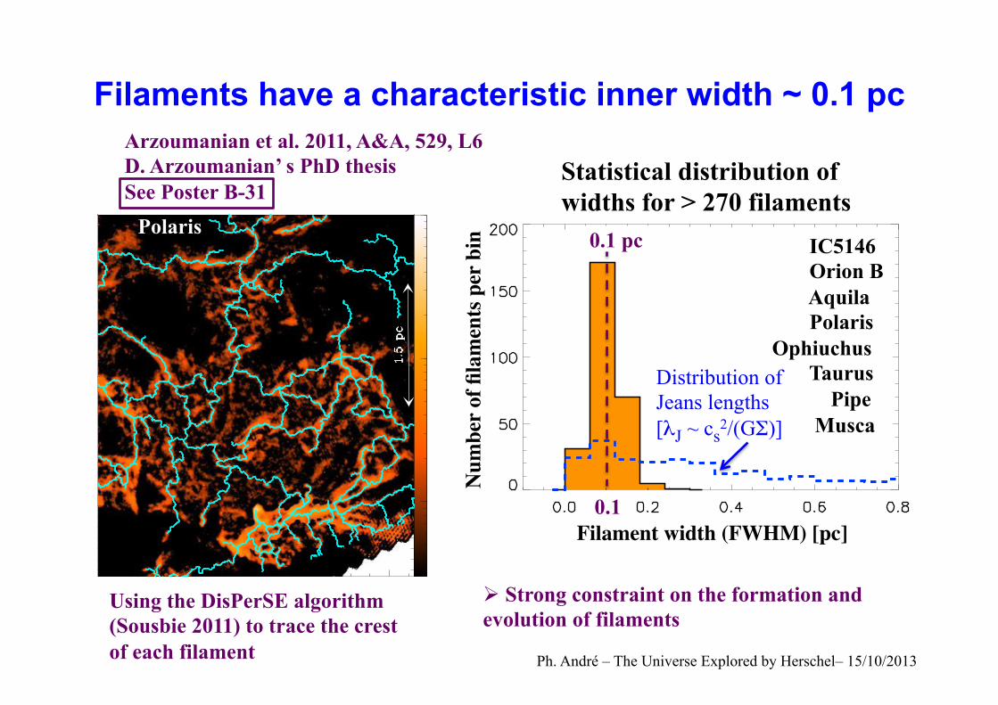
! Strong constraint on the formation and evolution of filaments
Using the DisPerSE algorithm (Sousbie 2011) to trace the crest of each filament
Polaris
Filaments have a characteristic inner width ~ 0.1 pc
Num
ber o
f fila
men
ts p
er b
in !
Filament width (FWHM) [pc] !
Statistical distribution of widths for > 270 filaments
0.1
0.1 pc IC5146 Orion B Aquila Polaris
Ophiuchus Taurus Pipe Musca
Distribution of Jeans lengths [λJ ~ cs
2/(GΣ)]
Arzoumanian et al. 2011, A&A, 529, L6 D. Arzoumanian’ s PhD thesis See Poster B-31
Ph. André – The Universe Explored by Herschel– 15/10/2013
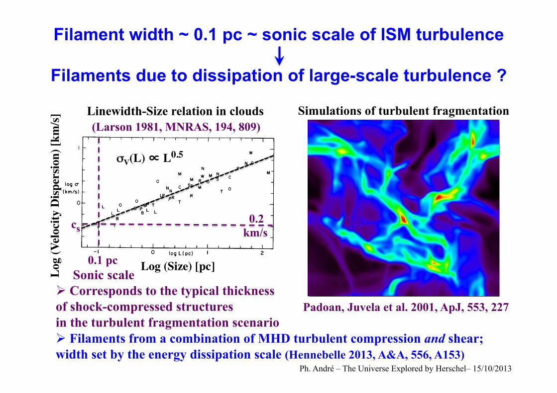
Filament width ~ 0.1 pc ~ sonic scale of ISM turbulence
Filaments due to dissipation of large-scale turbulence ?
! Corresponds to the typical thickness of shock-compressed structures in the turbulent fragmentation scenario
Turbulent Fragmentation, Padoan et al. (2001) structural resemblance to the observed filaments
Alexander Men’shchikov – ESLAB 2010 Symposium – May 4, 2010, Noordwijk – Page 61
column density Aquila in SPIRE bands, single scale ~40”
Simulations of turbulent fragmentation
Padoan, Juvela et al. 2001, ApJ, 553, 227
Linewidth-Size relation in clouds (Larson 1981, MNRAS, 194, 809)
1981MNRAS.194..809L
Log (Size) [pc] !Log
(Vel
ocity
Disp
ersio
n) [k
m/s]!
0.1 pc Sonic scale
0.2 km/s cs
σV(L) � L0.5
! Filaments from a combination of MHD turbulent compression and shear; width set by the energy dissipation scale (Hennebelle 2013, A&A, 556, A153)
Ph. André – The Universe Explored by Herschel– 15/10/2013

Filament width vs. Column density
Fila
men
t wid
th (F
WH
M) [
pc] !
Central column density NH2 [cm-2]!
Thermal Jeans length [λJ ~ cs
2/(GΣ)]
Arzoumanian et al. 2011, A&A, 529, L6 D. Arzoumanian’s PhD thesis
At low densities, consistent with model of polytropic filaments (P ~ ργ with γ~0.8) in pressure equilibrium with a typical ISM pressure Pext/kB ~ 5 × 10⁴ K cm-3 (Inutsuka, in prep.)!!See also Fischera & Martin 2012,
A&A, 542, A77 ! ! for a similar model for isothermal filaments!!
!
0.1
Unbound Self-gravitating
Ph. André – The Universe Explored by Herschel– 15/10/2013

Example of the B211/3 filament in the Taurus cloud (Mline ~ 54 M�/pc)
Palmeirim et al. 2013
VLSR~6 km/s
Velocity integrated CO intensity map
CO observations from Goldsmith et al. 2008
Herschel column density map
B211/3 filament
Evidence of accretion of background material (striations) onto self-gravitating filaments
Estimate of the mass accretion rate: Mline ~ 25-50 M�/pc/Myr Ph. André – The Universe Explored by Herschel– 15/10/2013

Filament width vs. Column density
Fila
men
t wid
th (F
WH
M) [
pc] !
Central column density NH2 [cm-2]!
Thermal Jeans length [λJ ~ cs
2/(GΣ)]
Arzoumanian et al. 2011 D. Arzoumanian’s PhD thesis
At high densities, consistent with a model of accreting filaments !(Hennebelle & André 2013, A&A)!
!!!!
!!!
! ! ! ! !
0.1 ! Balance between ‘accretion-driven turbulence’ (Klessen &
Hennebelle ’10) and dissipation of MHD turbulence due to ion-neutral friction
Unbound Self-gravitating
« Dynamical » equilibrium with <width> ~ 0.1 pc
Ph. André – The Universe Explored by Herschel– 15/10/2013
See also Heitsch 2013a,b!

~ 75 % of prestellar cores form in filaments, above a column density threshold NH2
> 7x1021 cm-2
Blow-up NH2 map (cm-2)
Examples of Herschel prestellar cores ( ) �
Σthreshold ~ 130 M�/pc2
<=> Av > 8 ~
Prestellar cores form primarily within filaments, above a column density threshold NH2 > 7x10²¹
cm-2
1021 1022 Aquila curvelet NH2
map (cm-2)
1
Unbound
Mline /M
line,crit 0.1
Unstable
Prestellar cores form primarily within filaments, above a column density threshold NH2 > 7x10²¹
cm-2
~
Prestellar cores form primarily within filaments, above a column density threshold NH2 > 7x10²¹
cm-2
André et al. 2010 + Könyves et al. 2010, A&A, 518!
Polychroni al. 2013, ApJL, in press!
Part of Orion A!
30’ ~
3.6
pc
See also Poster B-32 (M. Benedettini) for Lupus!Ph. André – The Universe Explored by Herschel– 15/10/2013

In Aquila, ~ 90% of the prestellar cores identified with Herschel are found above Av ~ 8 " Σ ~ 130 M� pc-2
Av ~ 8
Background column density, NH2 [1021 cm-2] !
N
umbe
r of c
ores
per
bin
: ΔN
/ΔΝ
H2!
Distribution of background column densities! for the Aquila prestellar cores!
Strong evidence of a column density “threshold” for the formation of prestellar cores
Könyves etal. in prep!André et al. IAU270!(astro-ph/1309.7762) ! ! !See also (for YSOs):!Heiderman ea. 2010!Lada et al. 2010
Ph. André – The Universe Explored by Herschel

! The gravitational instability of filaments is controlled by the mass per unit length Mline (cf. Ostriker 1964, Inutsuka & Miyama 1997):!
• unstable if Mline > Mline, crit!
• unbound if Mline < Mline, crit!
• Mline, crit = 2 cs2/G ~ 16 M�/pc
for T ~ 10K !
André et al. 2010, A&A Vol. 518
Interpretation of the star formation threshold
1021 1022 Aquila curvelet NH2
map (cm-2)
1
Unbound
Mline /M
line,crit 0.1
Unstable
� : Prestellar cores ! The gravitational instability of filaments is controlled by the mass per unit length Mline (cf. Ostriker 1964, Inutsuka & Miyama 1997):!
• unstable if Mline > Mline, crit!
• unbound if Mline < Mline, crit!
• Mline, crit = 2 cs2/G ~ 16 M�/pc
for T ~ 10K " Σ threshold!! Simple estimate: ! Mline� NH2 x Width (~ 0.1 pc)!
Unstable filaments highlighted in white in the NH2 map!
~ 160 M�/pc2
Interpretation of the threshold: Σ or M/L above which interstellar filaments are gravitationally unstable
Ph. André – The Universe Explored by Herschel– 15/10/2013
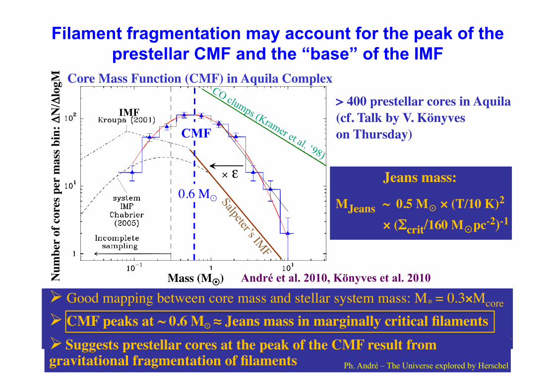
! Good mapping between core mass and stellar system mass: M* = ε Mcore with ε ~ 0.3 (cf. Motte et al. 1998; Alves et al. 2007)!! Cloud fragmentation models of IMF (Padoan & Nordlund; Hennebelle & Chabrier)!
Core Mass Function (CMF) in Aquila Complex!
IMF
× ε)
Num
ber o
f cor
es p
er m
ass b
in: Δ
N/Δ
logM!
Mass (M�)!
0.6 M�
CMF
André et al. 2010, Könyves et al. 2010
> 400 prestellar cores in Aquila (cf. Talk by V. Könyves on Thursday)!
!
!!Jeans mass: !
MJeans ~ 0.5 M� × (T/10 K)2 !× (Σcrit/160 M�pc-2)-1 !
! Good mapping between core mass and stellar system mass: M* = 0.3×Mcore !! CMF peaks at ~ 0.6 M� ≈ Jeans mass in marginally critical filaments!! Suggests prestellar cores at the peak of the CMF result from gravitational fragmentation of filaments!
Filament fragmentation may account for the peak of the prestellar CMF and the “base” of the IMF
Ph. André – The Universe explored by Herschel
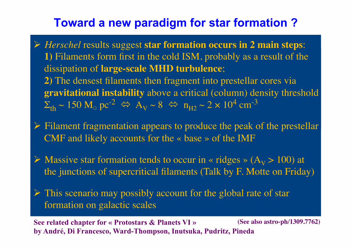
Toward a new paradigm for star formation ?
! Herschel results suggest star formation occurs in 2 main steps: 1) Filaments form first in the cold ISM, probably as a result of the dissipation of large-scale MHD turbulence; ! !!2) The densest filaments then fragment into prestellar cores via gravitational instability above a critical (column) density threshold Σth ~ 150 M� pc-2 " AV ~ 8 " nH2 ~ 2 × 104 cm-3!
!
!
!
! Herschel results suggest star formation occurs in 2 main steps: 1) Filaments form first in the cold ISM, probably as a result of the dissipation of large-scale MHD turbulence; ! ! 2) The densest filaments then fragment into prestellar cores via gravitational instability above a critical (column) density threshold Σth ~ 150 M� pc-2 " AV ~ 8 " nH2 ~ 2 × 104 cm-3!
! Filament fragmentation appears to produce the peak of the prestellar CMF and likely accounts for the « base » of the IMF!
! Massive star formation tends to occur in « ridges » (AV > 100) at the junctions of supercritical filaments (Talk by F. Motte on Friday)!
! This scenario may possibly account for the global rate of star formation on galactic scales!
!
!
!
See related chapter for « Protostars & Planets VI » by André, Di Francesco, Ward-Thompson, Inutsuka, Pudritz, Pineda
(See also astro-ph/1309.7762)

SFR (M�/yr) ! � ) 4.5 × 10�8 × Mdense(M�)
!
Mdense = Mass of dense gas above the threshold (Av > 8 or nH2 > 2.5 × 104 cm-3)
=) εcore × fpre × Mdense / tpre )
� ) 0.3 × 0.15 × Mdense(M�) / 106!
Herschel results on Aquila ! prestellar cores!
!Mdense = Mass of dense gas above the threshold (Av > 8 or nH2 > 2.5 × 104 cm-3)
André et al. 2011 (astro-ph/1309.7762)
HCN Gao & Solomon 2004
Lada et al. 2012!
AV > 8 mag Lada et al. 2010
Mass of dense gas (M�)!
Star
For
mat
ion
Rat
e (M�
yr-1
)!A universal star formation law above the threshold ?
normal spirals
LIRGs
ULIRGs