Goods Prices and Availability in Cities

Goods Prices and Availability in Cities

Jessie Handbury

University of Pennsylvania

David E. Weinstein∗

Columbia University and NBER

November 17, 2014

Abstract

This paper uses detailed barcode data on purchase transactions by households in 49

U.S. cities to calculate the first theoretically-founded urban price index. In doing so, we

overcome a large number of problems that have plagued spatial price index measurement.

We identify two important sources of bias. Heterogeneity bias arises from comparing dif-

ferent goods in different locations, and variety bias arises from not correcting for the fact

that some goods are unavailable in some locations. Eliminating heterogeneity bias causes

97 percent of the variance in the price level of food productsacross cities to disappear rel-

ative to a conventional index. Eliminating both biases reverses the common finding that

prices tend to be higher in larger cities. Instead, we find that price level for food products

falls with city size.

∗We wish to thank Paul Carrillo, Donald Davis, Jonathan Dingel, Gilles Duranton, Zheli He, Joan Monras,Mine Senses, and Jonathan Vogel for excellent comments. Molly Schnell and Prottoy Aman Akbar provided uswith outstanding research assistance. David Weinstein would like to thank the NSF (Award 1127493) for generousfinancial support. Jessie Handbury would like to thank the Research Sponsors’ Program of the Zell-Lurie RealEstate Center at Wharton for financial support.

1 Introduction

The variation in prices and price indexes across locations is as central to economic geography

and international economics as inflation is to macroeconomics. However, the methods used to

construct prominent spatial price indexes are significantly cruder than those used to construct

inflation rates and other inter-temporal price indexes. While the U.S. Consumer Price Index

(CPI) compares the relative prices over time of identical goods sold in the same store, regional

price indexes compare different (but similar) goods purchased in different stores.1 Moreover,

the U.S. CPI accounts for product entry and exit. Evidence suggests that product availability

varies across locations as well as over time, yet even the latest spatial price indexes do not

account for these differences.2

This paper uses detailed barcode data documenting purchasetransactions by households

in 49 U.S. cities to overcome these obstacles in spatial price index measurement. In order to

give some sense of the magnitude of the heterogeneity and variety biases in standard indexes,

we focus on two phenomena: the spatial variation in price indexes, which is itself the subject

of the purchasing power parity (PPP) debate, and the correlation of price indexes with popu-

lation, which yields a common agglomerating force across many New Economic Geography

(NEG) models. Our use of better data enables us to replicate prior results from these areas and

demonstrate a number of novel findings.

First, we precisely measure prices ofidentical goods sold in comparable stores across 49

U.S. cities to properly estimate spatial price differences. While standard price indexes show

a positive correlation between average prices and city sizes, this correlation almost entirely

disappears when we compare transaction prices of identicalproducts purchased in the same

stores. If we define purchasing power parity (PPP) deviations as differences in the average

price of traded goods, we find that 97 percent of the variance in PPP deviations for groceries

across U.S. cities can be attributed to heterogeneity biases in the construction of price indexes.

Second, while average product prices do not vary much acrossspace, we find dramatic

differences in product availability. The detail of our transaction-level data allows us to quantify

these differences. We estimate the number of varieties of products available in each city and find

that a doubling in city size is associated with a 20 percent increase in the number of available

products.

1The ACCRA (American Chamber of Commerce Researchers Association) index of U.S. urban prices, usedin important papers such as Chevalier (1995), Parsley and Wei (1996), Albouy (2009), and Moretti (2013), is anexample of such an index.

2The Bureau of Economic Analysis (BEA) recently released regional price (RPP) indexes for the U.S. The RPPmethodology, outlined in Aten (2005) and Aten and Martin (2012), makes some headway towards adjusting forproduct and store heterogeneity. Product heterogeneity has also been partially addressed in the latest Penn WorldTable (PWT), which compares quality-adjusted prices across countries (Feenstra et al., 2012). Data limitationsmean that neither the PWT or the BEA’s RPP indexes compare identical goods in different markets (which iscritical for the approach used in this paper), nor do they adjust for variety differences.

1

Finally, we use data on the purchase quantities, as well as transaction prices, to demonstrate

that the differences in variety availability yield economically significant variation in the price

level across cities.3 When we use the data to construct a theoretically rigorous price index that

corrects for product, purchaser, and retailer heterogeneity and accounts for variety differences

across locations, we find that the price level is actually lower in larger cities. Consumers spend

less, on average, to get the same amount of consumption utility in larger cities.

The association between city population and price levels plays an important role in many

urban and NEG models. NEG models typically predict that price indexes over tradable goods

are lower in larger cities (see,e.g.,Fujita (1988); Rivera-Batiz (1988); Krugman (1991); Help-

man (1998); Ottaviano et al. (2002); Behrens and Robert-Nicoud (2011)). This prediction is at

odds with empirical work demonstrating that prices are higher in larger cities (DuMond et al.,

1999; Tabuchi, 2001). One reason that these studies have notbeen deemed fatal for the theory is

that it is easy to modify NEG models to generate higher housing prices in cities (see,e.g.,Help-

man (1998)). Our paper suggests data problems in the construction of urban price indexes are

sufficiently large to explain the seemingly contradictory evidence: variety- and heterogeneity-

adjusted price indexes are lower in larger cities.

A key difference between this paper and earlier work is that we work with barcode data, so

the prices we compare are foridenticalgoods. Our dataset includes the prices for hundreds of

thousands of goods purchased by 33,000 households in 49 cities in the U.S. Critically, the data

indicate the price of each good, where it was purchased, and information about the purchaser.

Consistent with earlier analyses, if we aggregate our data and compare the prices ofcategories

of goods, we find that the elasticity of the grocery price level with respect to population is

0.042. This implies that New Yorkers (population 21.2 million) pay 16 percent more than

people in Des Moines (population 456,000) for similar, but not necessarily identical, groceries.

However, when we adjust this index, step-by-step, for the various biases we identify in the

standard methodology, we end up with our final estimate for the correct elasticity: -0.011.

When estimated properly, grocery price indexes do not rise,but rather fall, with population.

One of the most important classes of bias are “heterogeneitybiases,” which arise from

not being careful about which prices are being compared. Forexample, the price of an item

like a “half-gallon of whole milk” can vary enormously depending on a number of sources of

underlying heterogeneity. “Product heterogeneity biases” arise because there are many varieties

of whole milk that differ in price,e.g.,name brand vs. store brand, organic vs. non-organic, etc.4

“Retailer heterogeneity biases” arise because high-amenity stores may systematically charge

different prices to low-amenity stores for the same good. Finally, “purchaser heterogeneity

3We use the word “price” to refer to the price of a particular good and the term “price level” to refer to a priceindex, or some weighted average of relative prices across goods.

4Just to give one simple case of this, in Westside Market in NewYork on August 18, 2013, a half gallon ofFarmland whole milk sold for $2.47 while a half gallon of Sky Top Farms whole milk sold for $6.59.

2

biases” arise because shoppers who search intensely for thelowest price can often purchase the

same good in the same store for less. Regional price indexes typically do not correct for these

biases because without barcode data it is difficult to find thesame good in the same store chain

in two different locations.5 To get some sense of the magnitude of these biases among goods

that are available in more than one location, we regress disaggregate log prices against log

population with product, purchaser characteristic, and store controls. We find that controlling

for these heterogeneity biases reduces the elasticity of price with respect to population from

0.042 to 0.006 (86 percent). This indicates that the large positive elasticity in the aggregate data

is due to the fact that consumers in large cities tend to purchase higher quality varieties in nicer

stores and shop less intensely (presumably because rich people have a higher opportunity cost of

time). Although statistically different from zero, the elasticity that remains after controlling for

heterogeneity is not economically meaningful; it implies prices of commonly-available goods

are approximately equal in large and small cities. Indeed, between 95-97 percent of the variance

in PPP deviations across cities disappears once we correct for these biases.

A second major source of bias is variety bias. Variety biasesarise because consumers do not

have access to the same set of products in all locations. These biases have been studied in the

context of the CPI by Broda and Weinstein (2010), but there isreason to believe that they are

much more important in the regional context. The differencein product availability between

New York and Des Moines, for example, is likely to be much greater than the difference in

product availability in the U.S. economy from one year to thenext. In order to quantify this

effect, we adapt some well-developed statistical procedures to the problem of estimating the

number of varieties in cities. Our results indicate very large differences in variety availability.

We estimate that there are approximately four times more types of grocery products available

in New York than in Des Moines.

In order to quantify the variety bias we need to put more structure on the problem. We use

a spatial variant of the Constant Elasticity of Substitution (CES) exact price index developed in

the seminal work of Feenstra (1994). The CES structure is commonly employed in NEG models

and is well suited for our data.6 When calculated over varieties available in more than one city

and using prices adjusted for product, purchaser, and storeheterogeneity, the theoretically-

rigorous CES index yields almost the same elasticity of price with respect to population as the

price regression above. An advantage of the CES framework isthat it enables us to make an

additional adjustment for the fact that small cities offer consumers substantially fewer purchase

5The food component of the BEA RPP is based on BLS data. The BLS is careful to keep products and storesconstant over time, but uses random sampling to select the stores and products for which prices are collected ineach location. ACCRA provides field agents with detailed instructions to collect prices for products and in storesmeeting certain specifications. These instructions leave alarge scope for product and store heterogeneity in prices.

6Recent NEG models have also used the quadratic linear framework developed by Ottaviano et al. (2002).While quadratic linear framework is tractable for theoretical analysis, it is difficult to estimate and, therefore, notwell-suited for price index measurement.

3

options. Given the important difference in product availability across locations, we find that

variety bias is extremely important economically. Correcting for the variety bias further lowers

the elasticity of price with respect to city size to -0.011. In other words, when we correct for

heterogeneity and variety biases, the standard result thatprices rise with city size is reversed.

This paper complements large literatures studying international price and variety differ-

ences. Simonovska (2010) and Landry (2013), for example, use micro price data to document

international price differences of identical products. Barcode price data has also been used ex-

tensively in the study of PPP convergence (see a recent survey by Burstein and Gopinath (2013))

and PPP convergence (see,e.g., Broda and Weinstein (2008); Burstein and Jaimovich (2009);

Gopinath et al. (2011)). Hummels and Klenow (2005) documentthat larger countries export

more varieties of products; while Bernard et al. (2007) and Eaton et al. (2011) document that

larger countries import more varieties of products.

There is less work on intranational price and variety differences. Parsley and Wei (1996)

use the ACCRA data to examine convergence to the law of one price in the U.S. Crucini and

Shintani (2008) use similar data from the Economist Intelligence Unit, to examine the persis-

tence of law of one price deviations for nine U.S. cities. This work on deviations from the law

of one price does not address the question of how much of the difference in observed prices

across cities reflects unobserved heterogeneity in products or retailers. The only other paper, to

our knowledge, to compare prices of identical goods within countries is Atkin and Donaldson

(2012), who use spatial price differences as a proxy for intranational trade costs in developing

countries.

A nascent literature has documented that larger and more dense areas in the U.S. have more

varieties of restaurants (Schiff, 2012). Unfortunately, the lack of price data and the inability to

control for quality differences across restaurants in different locations make it difficult to accu-

rately measure the welfare implications of these variety differences. Recent work by Couture

(2013) uses household travel patterns to estimate the substitution between restaurants but, with-

out an additional price or quality measure, he cannot separately identify price from quality, and

so he must assume that these two factors are perfectly correlated.

In complementary work, Handbury (2012) uses the same data asthe current paper to cal-

culate variety-adjusted city-specific price indexes for households at different income levels and

finds that high-income households face relatively lower price indexes in cities with higher per

capita incomes. Consistent with the PPP variance results here, Handbury (2012) finds that these

intra-income differences are driven entirely by variety differences across cities. Both papers

point towards the relevance of the extensive variety marginin explaining PPP deviations across

cities.

The rest of the paper is structured as follows. Section 2 describes the data. Sections 3 and

4 explore how identical goods prices and goods availabilityvary across cities. In Section 5 we

4

summarize these results using an urban price index that adjusts for the heterogeneity and variety

biases in standard indexes. Section 6 concludes.

2 Data

The primary dataset that we use is taken from the Nielsen Homescan database. These data were

collected by Nielsen from a demographically representative sample of approximately 33,000

households in 52 markets across the U.S. in 2005.7 Households were provided with Universal

Product Code (UPC) scanners to scan in every purchase they made including online purchases

and regardless of whether purchases were made in a store withscanner technology.8 Each

observation in our data represents the purchase of an individual UPC (or barcode) in a particular

store by a particular consumer on a particular day. We have the purchase records for grocery

items, with information on the purchase quantity, pre-tax price, and date; the name or type of

the store where the purchase is made; and demographic information on the household making

the purchase.9

Figure 1 presents the basic structure of our data. A barcode,u, uniquely identifies a prod-

uct. For example, “Horizon 1% Milk in a Half-Gallon Container” has a different barcode than

“Horizon 2% Milk in a Half-Gallon Container.” Nielsen provides product characteristics for

each barcode, including its brand, a detailed product-typedescription that Nielsen refers to as

a “module,” and a more aggregate product-type description that Nielsen refers to as a prod-

uct “group.” For example, “Horizon 1% Milk in a Half-Gallon Container” is sold under the

“Horizon” brand in the “Milk” module within the “Dairy” product group. We group barcodes

with the same brand and in the same module into “brand-modules.” For example, “Horizon

Milk,” “Horizon Butter,” and “Breakstone Butter,” constitute three different brand-modules in

the “Dairy” product group, the first of which is in the “Milk” module and the latter two are in

the “Butter” module. The 2005 Homescan sample we consider contains transaction records for

almost 350,000 UPCs that are categorized into 597 modules, 27,853 brands, and 55,559 brand-

module interactions and 63 product groups.10 Detailed descriptions of the Nielsen data and the

7The Nielsen sample is demographically representative within each market.8In cases where panelists shop at stores without scanner technology, they report the price paid manually. Since

errors can be made in this reporting process, we discard any purchase records for which the price paid was greaterthan twice or less than half the median price paid for the sameUPC, approximately 250,000 out of 16 millionobservations.

9Nielsen provides a store code for each transaction in the data. For all but 800,000 of 16 million transactions,the store code identifies a unique store name. For the remaining observations representing 4.4 percent of sales inthe data, Nielsen’s store code refers to one of approximately 60 store categories, such as “Fish Market,” “CheeseStore,” “Drug Store,” etc.

10This sample excludes the “random weight” product group. Thequality of random weight items, such asfruit, vegetables, and deli meats, varies over time as the produce loses its freshness. We cannot control for thisunobserved quality heterogeneity.

5

sampling methods used can be found in Broda and Weinstein (2010).

Figure 1: Terminology

Universal Product Code (UPC) or Barcode⊂ Brand-Module ⊂ Product Group

(u∈Ug) (b∈ Bg) (g∈ G)

e.g.Horizon 1% Milk in a e.g.Horizon Milk e.g.Dairy

Half-Gallon Container

N=348,646 N = 55,559 N = 63

Although the Nielsen dataset contains data for 52 markets, we classify cities at the level

of Consolidated Metropolitan Statistical Area (CMSA) where available and the Metropolitan

Statistical Area (MSA) otherwise. For example, where Nielsen classifies urban, suburban, and

ex-urban New York separately, we group all three together asthe “New York-Northern New

Jersey-Long Island CMSA”. We use population, income distribution, and racial and birthplace

diversity data from the 2000 U.S. Census and 2005 retail rents from REIS.11,12 The population

and retail rents for the cities included in the analysis are listed in Table A.1, along with market

IDs we will use to identify cities in the charts below. There are two cases in which Nielsen

groups two MSAs into one market. In these cases, we count the two MSAs as one city, using

the sum of the population and the population-weighted mean retail rents.

3 Measuring Retail Prices in Cities

While our ultimate goal is to construct a theoretically-founded urban price index, we begin by

exploring the data. Variation in the price index across cities is driven by differences in the prices

of identical goods and the variety availability. Our reduced-form analysis explores each of these

factors. In this section, we focus only on the price data. We address goods availability and the

construction of an urban price index in Sections 4 and 5, respectively.

3.1 Evidence From Categories of Goods

A common method to compare price levels across cities withincountries relies on unit value in-

dexes such as those published by the Council for Community and Economic Research (formerly

11Specifically, we use the combined effective rents for community and neighborhood shopping centers. Effectiverents adjust for lease concessions.

12We replicated the analysis below using total manufacturingoutput and food manufacturing output as alterna-tive measures of city size and reached the same qualitative conclusions. This is not surprising, as the data for totalmanufacturing output and food manufacturing output from the 2007 U.S. Economic Census were highly correlatedwith population across the cities in our sample, with coefficients of 0.70 and 0.73, respectively.

6

the American Chamber of Commerce Research Association (ACCRA)). ACCRA collects prices

in different cities across the U.S. for a “purposive” (i.e., non-random) sample of items that is se-

lected to represent categories of goods. For each item, ACCRA’s price collectors are instructed

to record the price of a product that meets certain narrow specifications,e.g., “half-gallon whole

milk,” “13-ounce can of Maxwell House, Hills Brothers, or Folgers ground coffee,” “64-ounce

Tropicana or Florida Natural brand fresh orange juice,” etc. ACCRA takes the ratio of the aver-

age price collected for each item in each city and quarter relative to its national average in that

quarter. The ACCRA COLI is a weighted average of these ratios, where item weights are based

on data from the U.S. Bureau of Labor Statistics 2004 Consumer Expenditure Survey.13

There are a host of problems arising from comparing prices ofsimilar (as opposed to iden-

tical) products; we deal with these in Section 3.3. As a baseline, we first replicate the standard

result that, if one uses the standard ACCRA methodology, theprice index for tradable goods

rises with population in our data. In order to establish thisstylized fact, we obtained the ACCRA

COLI data for 2005 and measured the association between log population and four different in-

dexes: ACCRA’s aggregate, or composite, cost-of-living index; their grocery index; and two

food price indexes that we built using the ACCRA item-level price ratios and weights. We re-

fer to these two constructed indexes as the ACCRA food index and Nielsen food index. The

ACCRA food index is a weighted average of item-level relative prices, using ACCRA’s price

ratios and weights, but only for food items. The Nielsen foodindex replicates the ACCRA food

index by applying the ACCRA methodology to Nielsen price data. To build this index, we first

identified the set of UPCs in the Nielsen data whose characteristics match the ACCRA speci-

fications for each food item represented in the ACCRA index. We then calculated the average

price observed in the Nielsen data for the set of UPCs matching each item in each city and the

ratio of each of these city-specific item unit values to theirnational average. The Nielsen food

index for each city is the weighted average of these Nielsen unit value ratios across items using

ACCRA item weights.

Table 1: Category Price Indexes vs. Population

ACCRA Price Indexes Ln(Nielsen

Ln(Composite Indexc) Ln(Grocery Indexc) Ln(Food Indexc) Food Indexc)

[1] [2] [3] [4]Ln(Populationc) 0.132*** 0.0727*** 0.0718*** 0.0423***

[0.0209] [0.0167] [0.0168] [0.00939]Constant 2.706*** 3.562*** 3.541*** 3.982***

[0.306] [0.245] [0.245] [0.138]Observations 47 47 47 47R-Squared 0.47 0.30 0.29 0.31

Standard errors in brackets; *** p<0.01, ** p<0.05, * p<0.1.

13See http://www.coli.org/Method.asp for more details.

7

We regressed the log of each price index for each city on the log of the city’s population

and report the results in Table 1. As one can see from the table, there is a very strong positive

association between each of these price indexes and population. Although the composite AC-

CRA index, which includes land prices, rises the steepest with population, we see a very similar

pattern for the grocery and food price indexes. A one log-unit rise in city size is associated with

a four percent increase in the food price index when we build it using Nielsen data and seven

percent when we rely on the ACCRA data. While the magnitude ofthe slope coefficient varies

across the indexes, none of these differences are statistically significant.14 The coefficients are

also economically significant: the smallest coefficient, from the Nielsen price index regression,

suggests that a consumer in New York pays 16 percent more for food items than a person in Des

Moines.15

3.2 Controlling for Product, Buyer, and Retailer Heterogeneity

There are three types of heterogeneity biases that may generate the positive correlations ob-

served above: product heterogeneity bias, retailer heterogeneity bias, and purchaser hetero-

geneity bias. If consumers in larger cities systematicallypurchase higher quality (i.e., more

expensive) varieties within a product category, then a higher average price level in a city might

just reflect the fact that consumers in that city buy more expensive varieties of that product cat-

egory. Similarly, retailer heterogeneity bias can arise because consumers in large cities might

purchase goods in stores that offer systematically higher amenities. For example, some grocery

stores, like Whole Foods, offer nicer shopping experiencesthan mass-merchandisers. Finally,

if there is a higher fraction of wealthy people in large cities, and rich people bargain-shop less

than poor people, purchaser heterogeneity might mean that purchase prices may reflect different

shopping intensities of consumers.

As we mentioned earlier, our objective is obtain a standardized price measure that reflects

the prices of identical goods purchased in different locations but at similar stores and by con-

sumers with similar shopping intensities. Essentially, weare trying to do the spatial equivalent

of the time-series methodology employed in the construction of the U.S. Consumer Price In-

dex, which measures price changes for identical products, purchased in the same store, by field

agents with common shopping instructions.

Our methodology for doing this is quite straightforward. Let Pucrh be the average price that

14This partially reflects the fact that the correlation coefficient between the various price indexes ranges from0.8 to 0.9.

15Other indexes show a similar pattern. When we regress the BEARPP index for goods against log populationusing our sample of cities, the coefficient on log populationis 0.026 and statistically significant at the 1 percentlevel. There are many potential reasons for the difference between this elasticity and those reported in Table 1,including that the RPP covers a different, broader set of goods than we have in the Nielsen data and partially adjustsfor product and store heterogeneity.

8

a householdh paid for UPCu in storer in city c.16 We referPucrh as the “unadjusted price”

and definepucrh as ln(Pucrh). We can then construct an adjusted price index by running the

following regression:

pucrh = αu+αc+αr +Zhβ + εucrh (1)

whereαu, αc, andαr are UPC, city, and store fixed effects, respectively;Zh denotes a vector

of household characteristics; andβ is a vector of corresponding coefficients. Household demo-

graphic dummies are included for household size, as well as the gender, age, marital status, and

race of the head of household; in addition, we control for household income, which is correlated

with shopping intensity. Our store fixed effects take a different value for each of the approx-

imately 600 retail chains in our sample that serve at least 2 cities. For stores that we observe

serving a single city, we restrictαr to be the same for all stores of the same type, where type

is defined in one of seven “channel-IDs”: grocery, drug, massmerchandiser, super-center, club,

convenience, and other.17 Theαr are designed to capture store amenities, and theZhβ capture

factors related to purchaser heterogeneity.

The city fixed effects,αc, can be thought of as city price indexes that control for the types

of products purchased, the store in which the purchase occurred, and the shopping intensity

of the buyer. We then can test whether standardized urban prices co-vary with population by

regressing the city fixed effects on log population,i.e.,

αc = α + γ ln(Popc)+ εc, (2)

where ln(Popc) is the log of population in cityc. In this specification,γ tells us how prices vary

with population after we control for the different bundles of products purchased in different

cities. An advantage of this two-stage approach as opposed to simply including co-variates of

interest in equation (1) is that our city price level estimates are not affected by what we think

co-varies with urban prices.18 Thus, we separate the question of whether urban prices rise with

population from the question of how to correctly measure urban prices. We will use this feature

of the methodology in Section 5.

16Homescan panelists record purchases for each transaction they make while participating the survey and datarecords are identified using a calendar date. We aggregate the data to the annual frequency, summing purchasevalues and quantities across transactions in the 2005 sample. The average price paid is, therefore, the sum ofthe dollar amounts that a householdh paid for UPCu in storer over all of the transactions where we observethe household purchasing that UPC in that store, divided by the sum of the number of units that the householdpurchased across the same set of transactions. We identify the “store”r that a transaction occurs in using Nielsen’sstore code variable.

17We apply the same restriction to stores whose codes refer to store categories (such as “Fish Market,” “CheeseStore,” etc.) rather than store names.

18In the Handbury and Weinstein (2011) we show that we obtain qualitatively similar results if we use a one-stepprocedure including population in equation 1.

9

3.3 Evidence from Barcode Prices

Recall that in Section 3.1 above, we showed that products from the same category were pur-

chased for higher unit values in larger cities. The results in Table 1 indicated that a one log

unit rise in city size is associated with a four percent rise in the unit value of groceries. We

will now demonstrate that almost all of this effect can be explained by product, retailer, and

purchaser heterogeneity biases. In other words, the findingin past studies that there are higher

traded goods prices in larger cities arises because big cities have different (less price sensi-

tive) consumers purchasing different (more expensive) varieties of products in different (more

expensive) stores.

Table 2 presents results from estimating equations (1) and (2). The first key difference from

Table 1 is that we are now gauging price differences between identical products, or UPCs, sold

in different cities.19 In the first column of the table, we present the results from a specification

that only adjusts for product heterogeneity. In other words, instead of running the regression

specified in equation (1), we compute the city price index by only regressing prices on UPC and

city dummies. This method for computing the price index corrects for product heterogeneity,

which is contained in the UPC fixed effects, but does not adjust for purchaser and retailer

heterogeneity. In the second panel, we report the results from regressing the estimated city

dummy coefficients on log population. We obtain a coefficientof 0.0139, which is only one

third as large as the coefficient we obtained in Table 1 when weused the ACCRA methodology

to generate a price index and regressed that on population. This result indicates that two-thirds

of the positive relationship between prices and city size inthe unit value index reflects the fact

that people in larger cities purchase far more high-priced varieties of goods than residents of

small cities.20

In Column 2 of Table 2, we adjust the urban price index for bothproduct heterogeneity

and purchaser heterogeneity. The positive coefficient on household income indicates that high

income households systematically pay more than poorer households for the same goods. Some

of this may be due to the fact that high-income households have either a higher opportunity

cost of time (and therefore shop less intensively) and/or a greater willingness to shop in high

amenity stores. Alternatively, some of this positive association may be due to the fact that

stores that cater to richer clientele are able to charge higher markups. While we will disentangle

these forces in Section 3.4, for the time being we simply notethat controlling for purchaser

heterogeneity causes the coefficient on log population to fall by another ten percent.

19In all regressions, we weight the data by the transaction value which gives more weight to goods that constitutehigher expenditure shares.

20One possible concern with these results is that shifts in theweighting of the data or some other factor associatedwith the shift from the price index methodology to the regression methodology is responsible for the drop. Weinvestigate this possibility as a robustness check and showin the Appendix C of Handbury and Weinstein (2011)that this concern is not warranted.

10

Table 2: Identical Product Price Indexes vs. Population

Panel A

p1ucrh

[1] [2] [3] [4]Ln(Incomeh) - 0.0114*** - 0.00805***

- [0.000961] - [0.000525]

UPC Fixed Effects Yes Yes Yes YesCity Fixed Effects Yes Yes Yes YesHousehold Demographic Dummies2 No Yes No YesStore Dummies3 No No Yes Yes

Observations 15,570,529 15,570,529 15,570,529 15,570,529Number of UPCs4 348,645 348,645 348,645 348,645R-Squared 0.948 0.948 0.953 0.953

Panel B

City Fixed Effect Coefficient from Panel A

[1] [2] [3] [4]Ln(Populationc) 0.0139*** 0.0130*** 0.00603*** 0.00568**

[0.00400] [0.00396] [0.00215] [0.00214]Constant -0.245*** -0.229*** -0.117*** -0.110***

[0.0586] [0.0581] [0.0315] [0.0314]

Observations 49 49 49 49R-Squared 0.916 0.205 0.187 0.143

Standard errors in brackets; *** p<0.01, ** p<0.05, * p<0.1.Panel A standard errors are clustered by city.

Notes:1. pucrh = ln(Pucrh) wherePucrh is the total expenditures by householdh on UPCu in storer in city c in 2005 divided bythe total quantity of UPCu purchased by householdh in storer in city c during 2005. Observations in thePanel A regression are weighted by the total expenditure of householdh on UPCu in storer.2. Household demographic dummies are for household size, male and female head of household age, marital status,race, and hispanic.3. Regressions with store dummies include one of seven channel-ID dummies is Nielsen does not provide a store nameor the store identified only has sales in one city and a store name dummy otherwise.4. Random weight UPCs have been dropped from the sample.

Interestingly, controlling for store fixed effects in Column 3 has a much more substantial

impact on the elasticity of urban prices with respect to population than controlling for purchaser

heterogeneity: more than halving the coefficient. The largeimpact of controlling for store

heterogeneity implies that a second important reason why prices appear higher in larger cities is

that residents of large cities disproportionately shop in stores that charge high pricesin all

cities. The most obvious source of this sort of heterogeneity is differences in amenities—

rich households living in big cities tend to purchase nicer varieties of goods and shop in nicer

stores—but we will also examine the possibility that markupvariations are explaining this in

Section 3.4.

Finally, if we control for product, purchaser, and retailerheterogeneity in Column 4 the

11

coefficient collapses to only 13 percent of its magnitude in Table 1. Most of this fall arises

from adjusting for retailer heterogeneity, which reflects that shoppers in larger cities purchase

more items in high-amenity stores. The coefficient on household income remains positive and

significant, which means that richer households pay more forthe same UPCeven in the same

store.We interpret this as evidence for the impact of purchaser heterogeneity on observed trans-

action prices. Interestingly, the magnitude of the coefficient on income in Column 4 is about 70

percent as large as in Column 2, indicating that most of the reason why richer households pay

more for the same UPC is due to their lower shopping intensitywithin stores and not to their

choosing to shop in nicer stores.

Figure 2: Estimated Price Levels vs. Log City Population

DMLR

Oma

SyrAlb

Bir

Ric

Lou

GR

Jac

Mem

R−DNas

SLC

Cha

Col

SA

Ind

OrlMil

NH

KC

NO

OkCCin

Por

B−RPitTam

DenStL

SD

Cle

Pho

Sea

Mia

Atl

Hou

Dal

Det

Bos

Phi

SF

DC

Chi

LA NY

−.2

0.2

.4P

rice

Inde

x

13 14 15 16 17ln(City Population)

Adjusted Nielsen Price Index Nielsen Food Price Index

Notes:

1. The market labels on the ACCRA price indexes reference thecity represented, as listed in Table A.1.

2. City price indexes are normalized to be mean zero.

Figure 2 presents plots of price indexes computed using the ACCRA methodology in pre-

sented in the final column of Table 1 and the price indexes generated in Column 4 of Table 2.

The hollow circles indicate the price indexes computed using the ACCRA methodology and the

solid circles indicate those computed after correcting forthe various forms of heterogeneity in

the data. As one can see from the plot, there is a dramatic collapse in the relationship between

urban prices and population once one controls for product, purchaser, and retailer heterogene-

ity. Indeed, the slight positive association that we identified in Table 2 is almost imperceptible,

indicating that its economic significance is minor. Moreover, most of the dispersion in city price

indexes disappears once we control for heterogeneity yielding relatively small deviations from

the fitted line. In fact, adjusting for the various forms of heterogeneity bias, the variance in

urban price levels falls by 95 percent. This suggests that purchasing price parity for tradables

12

holds almost perfectly across US cities.

3.4 Amenities vs. Mark-ups

One of the important adjustments that we make is for store amenities. Our methodology as-

sumes that if consumers in a given city pay more for identicalproducts when they buy them

at one type of store relative to other stores within the same city, the higher price must reflect

a difference in store amenities. An alternative explanation is that the higher price reflects a

higher markup. If stores that are prevalent in larger citiescharge higher markups, our results

might be due to the fact that our method of eliminating retailer heterogeneity would be eliminat-

ing markup variation across cities and therefore might be understating the high prices in large

cities. In other words, if the store effects capture amenities, consumers do not necessarily find

big cities to be more expensive because they are getting a higher-quality shopping experience

in return for paying a higher price. If the store effects instead reflect markup differences due

to differences in market power across stores offering the same shopping experience, then con-

sumers are not getting anything in return for the relativelyhigh prices charged by stores in large

cities and will, therefore, perceive these stores as more expensive.

Although we cannot measure markups directly, we can look at store market share informa-

tion in an attempt to assess how markups might vary in our data, first across cities, and then

across retailers and, in particular, across retailers thatlocate disproportionately in large, rela-

tive to small, cities. In many variable markup demand systems involving strategic substitutes,

markups positively covary with market shares. For example,Feenstra and Weinstein (2010)

show that for the translog system, markups will positively covary with the Herfindahl index

in the market. We can compute retailer Herfindahl indexes foreach city by aggregating the

purchases of consumers in each store. Not surprisingly, Herfindahl indexes are negatively cor-

related with city size(ρ =−0.3) reflecting the fact that consumers in large cities not only have

more choices of products, but also more choices of where to purchase those products. This cir-

cumstantial evidence suggests that, if anything, we are understating the amenity effect because

stores in large cities are likely to face more competition and charge lower markups (which is

also consistent with models like Melitz and Ottaviano (2008)).

We also can try to strip out the market power effect from our estimates more directly. In

order to do this we control for differences in markups acrossretail chains, or types, by including

store market shares in the regression where we estimate the store effects (αr ).21 Specifically,

21Recall thatr denotes the store code for each transaction. Most store codes uniquely identify retail chains orstandalone stores; others refer to one of 60 store categories. If a store only has sales in one city or we do not havethe store name, we restrictαr to be equal across stores with the same “channel-ID,” which can take one of sevenvalues: grocery, drug, mass merchandiser, super-center, club, convenience, and other. We do not group stores inthis manner when calculating market shares:Sharerc represents the sales share of store coder in city c.

13

we add the market share of each store in each city to equation (1) and estimate

pucrh = αu+αc+αr +Zhβ + γSharerc + εucrh, (3)

whereSharerc is storer ’s market share in cityc and γ is a parameter to be estimated. We

interpretαr in this specification as the component of the store’s idiosyncratic price that cannot

be explained by its market power. We then subtract theseαr estimates from observed prices,

adjusting prices for the component that is potentially related to differences in amenities, but not

the component related to differences in markups via market power. We regress these adjusted

prices against city fixed effects to estimate urban price indexes that control for differences in

amenities across stores, but still allow for price differences resulting from differences in market

power:

pucrh− αr = αu+ αc+Zhβ + εucrh, (4)

The dependent variable is the store amenity-adjusted priceandαc is an urban price index that

reflects systematic differences in prices across stores with different market shares, but not those

related to unobserved heterogeneity between retail chains.

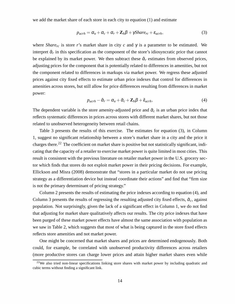
Table 3 presents the results of this exercise. The estimatesfor equation (3), in Column

1, suggest no significant relationship between a store’s market share in a city and the price it

charges there.22 The coefficient on market share is positive but not statistically significant, indi-

cating that the capacity of a retailer to exercise market power is quite limited in most cities. This

result is consistent with the previous literature on retailer market power in the U.S. grocery sec-

tor which finds that stores do not exploit market power in their pricing decisions. For example,

Ellickson and Misra (2008) demonstrate that “stores in a particular market do not use pricing

strategy as a differentiation device but instead coordinate their actions” and find that “firm size

is not the primary determinant of pricing strategy.”

Column 2 presents the results of estimating the price indexes according to equation (4), and

Column 3 presents the results of regressing the resulting adjusted city fixed effects,αc, against

population. Not surprisingly, given the lack of a significant effect in Column 1, we do not find

that adjusting for market share qualitatively affects our results. The city price indexes that have

been purged of these market power effects have almost the same association with population as

we saw in Table 2, which suggests that most of what is being captured in the store fixed effects

reflects store amenities and not market power.

One might be concerned that market shares and prices are determined endogenously. Both

could, for example, be correlated with unobserved productivity differences across retailers

(more productive stores can charge lower prices and attain higher market shares even while

22We also tried non-linear specifications linking store shares with market power by including quadratic andcubic terms without finding a significant link.

14

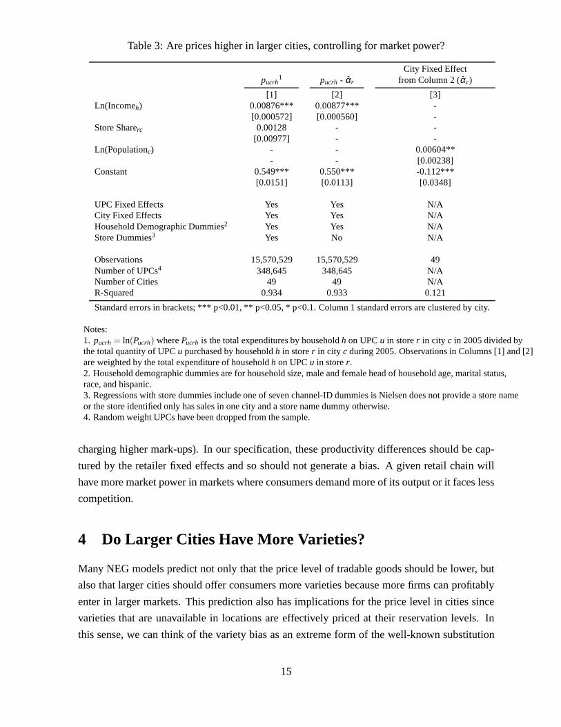
Table 3: Are prices higher in larger cities, controlling formarket power?

City Fixed Effectpucrh

1 pucrh - αr from Column 2 (αc)

[1] [2] [3]Ln(Incomeh) 0.00876*** 0.00877*** -

[0.000572] [0.000560] -Store Sharerc 0.00128 - -

[0.00977] - -Ln(Populationc) - - 0.00604**

- - [0.00238]Constant 0.549*** 0.550*** -0.112***

[0.0151] [0.0113] [0.0348]

UPC Fixed Effects Yes Yes N/ACity Fixed Effects Yes Yes N/AHousehold Demographic Dummies2 Yes Yes N/AStore Dummies3 Yes No N/A

Observations 15,570,529 15,570,529 49Number of UPCs4 348,645 348,645 N/ANumber of Cities 49 49 N/AR-Squared 0.934 0.933 0.121

Standard errors in brackets; *** p<0.01, ** p<0.05, * p<0.1.Column 1 standard errors are clustered by city.

Notes:1. pucrh = ln(Pucrh) wherePucrh is the total expenditures by householdh on UPCu in storer in city c in 2005 divided bythe total quantity of UPCu purchased by householdh in storer in city c during 2005. Observations in Columns [1] and [2]are weighted by the total expenditure of householdh on UPCu in storer.2. Household demographic dummies are for household size, male and female head of household age, marital status,race, and hispanic.3. Regressions with store dummies include one of seven channel-ID dummies is Nielsen does not provide a store nameor the store identified only has sales in one city and a store name dummy otherwise.4. Random weight UPCs have been dropped from the sample.

charging higher mark-ups). In our specification, these productivity differences should be cap-

tured by the retailer fixed effects and so should not generatea bias. A given retail chain will

have more market power in markets where consumers demand more of its output or it faces less

competition.

4 Do Larger Cities Have More Varieties?

Many NEG models predict not only that the price level of tradable goods should be lower, but

also that larger cities should offer consumers more varieties because more firms can profitably

enter in larger markets. This prediction also has implications for the price level in cities since

varieties that are unavailable in locations are effectively priced at their reservation levels. In

this sense, we can think of the variety bias as an extreme formof the well-known substitution

15

bias that plagues fixed-weight price indexes—if prices are so high that goods are not consumed

in small cities, fixed-weight indexes will understate the true cost of living because high-priced

goods that are not consumed will receive a weight of zero in the index. We will deal with

both the substitution and variety biases in Section 5. In this section we examine the underlying

evidence on variety availability.

4.1 Data Overview

The simplest way to document that consumers in larger citiesconsume more varieties is to

examine whether we observe more varieties being purchased in larger cities. Figure 3 shows

the relationship between the log of the number of UPCs observed in the Nielsen sample for

each city against log population. This relationship is upward sloping with a coefficient of 0.312

and standard error of 0.043. We cannot interpret this estimate as the elasticity of variety with

respect to city size, however, because Nielsen tends to sample more households in larger cities,

so part of the reason why more goods are purchased in larger cities is due to the greater sample

sizes in those cities.

Figure 3: Log Number of Distinct UPCs in Each City Sample vs. Log City Population

DM

LR

Oma

Syr Alb

Bir

Ric

Lou

GR

Jac

Mem

R−D

Nas

SLC

ChaCol

SA

IndOrl

Mil

NHKC

Sac

NOOkC

Cin

Por

B−R

Pit

TamDenStL

SD

Cle

MinPhoSeaMia

AtlHouDal

DetBos

Phi

SF

DC

ChiLA

NY

1010

.511

11.5

Ln(N

umbe

r of

UP

Cs)

13 14 15 16 17Ln(Population)

Ln(No. of Distinct UPCs Purchased by Sample HHs) Fitted values

Notes:

1. Numbers on plots reference the market ID of the city represented, as listed in Table A.1.

One way to deal with this bias is to instead examine whether the number of different varieties

consumed by an equal number of households varies with city size. The basic idea is that any two

households are less likely to purchase the same product in cities where there are more products

to choose from. If there is less overlap in the varieties purchased by different households in

larger cities, we expect to see equally-sized samples of households from these cities purchasing

larger numbers of unique varieties.

16

Here, we restrict ourselves to only looking at 25 cities in which Nielsen sampled at least 500

households and compare the number of varieties purchased bya random sample of 500 house-

holds in each of these cities.23 Figure 4 plots the aggregate number ofdifferentUPCs purchased

by these randomly-selected households against the size of the city in which the households live.

The results show a clear positive relationship between the variety of UPCs purchased by 500

households in a city and the population of the city. The slopeof the linear regression fit is 0.033

with a standard error of 0.017. The large amount of noise in the 500-household variety counts

indicates that this estimate may be subject to attenuation bias.24

These results are certainly suggestive of the notion that the number of varieties available

in a location rises with number of inhabitants in that location, but neither provides a reliable

estimate of the elasticity. In the next section, we take a more direct approach to estimating the

variety-city size relationship: we use all of the information at hand to estimate the total number

of varieties available in each location and then examine howthese aggregate variety estimates

vary with city size.

4.2 Estimating the Number of Varieties in Cities

The principle challenge that we face in measuring the numberof varieties in a city is that our

data is not a census of all varieties purchased in a city but rather a count of varieties based

on a random sample of households. Fortunately, our problem is isomorphic to a well-studied

problem in biostatistics: estimating the number differentspecies in a general area based on the

number of species identified in certain locations (see Mao etal. (2004, 2005)). Prior work in this

area has solved the problem using parametric and structuralapproaches that yield very similar

results in our data. Since the parametric approach is significantly simpler to explain, we focus

23There is a trade-off between the number of households that weconsider and the number of cities that can beincluded in the sample. As we decrease the number of households selected, we increase the number of cities inour sample (adding small cities disproportionately). However, as we work with smaller samples of households, wehave a lot more noise because the number of barcodes purchased by a small sample of households can vary a lotdepending on the households picked. This results in attenuation bias.

24We have replicated this analysis looking at the purchases ofdifferent fixed numbers of households and, con-sistent with the attenuation bias hypothesis, we find that the estimated variety-city size relationship is increasingin the number of households under consideration. For example, the coefficient on city size is statistically zerowhen we consider the number of varieties purchased by samples of 116 households in all 49 cities, but increasesto 0.05, statistically significant at the 5 percent level, when we look at the number of varieties purchased by 750households, in the 23 cities where this is possible.

One reason why it is difficult to identify differences in the number of varieties available in a city in the purchasesof small samples of households is due to the fact that many households purchase “popular” goods that otherhouseholds in their city also purchase. To see the intuitionhere, suppose that all households purchaseN+ 1products,N of which are the same across households in a city and one of which is drawn at random from the set ofvarieties available in the city. Regardless of how many varieties are available for purchase in a city, we can at mostexpect to seeN+1 unique varieties purchased by one household,N+2 by two households in the same city,N+3by three, etc. The number of varieties purchased in a city will range fromN to N plus the number of householdssampled in a city.

17

Figure 4: Log Number of Distinct UPCs Purchased by 500 Households in Each City vs. LogCity Population

Bir

Cha

Col

SA

Sac

OkC

B−R

TamDenStL

Min

PhoSea

Mia

Atl

Hou

Dal

Det

Bos

Phi

SF

DC

Chi

LA

NY

10.6

510

.710

.75

10.8

10.8

510

.9Ln

(Num

ber

of U

PC

s)


Ln(No. of Distinct UPCs Purchased by 500 HHs) Fitted values

Notes:

1. Numbers on plots reference the market ID of the city represented, as listed in Table A.1.

on the parametric approach and relegate the structural approach to Appendix A as a robustness

check.

In order to obtain some intuition for this methodology, assume that the expected number

of different products purchased by one household in cityc is denoted bySc(1). The expected

number of distinct products purchased in a sample ofn households can be denoted by the “accu-

mulation curve,”Sc(n). Accumulation curves must be concave because every time thesample

size rises by one household the probability of finding good that has not been purchased by any

of the other households falls. Moreover, a critical featureof accumulation curves is that as the

number of households surveyed rises, the number of observedvarieties in a city must approach

the true total number of varieties in a city. We can write thisformally as limn→∞ Sc (n) = STc ,

whereSTc is the total number of distinct varieties available in the city.25 In other words, the

asymptote of the accumulation curve is the estimate for the total number of goods available in

the city.

Estimation ofSTc requires us to know the expected value of distinct varietiesfor each sample

of households,i.e., (Sc(1),Sc(2),Sc(3), . . .), and also the functional form ofSc (n). Estimat-

ing the expected number of distinct varieties purchased by asample ofn households,Sc(n) is

straightforward. The only econometric issue we face is thatthe number of distinct varieties

we observe being purchased,Sc(n), in a sample ofn households is going to depend on exactly

which households are in the sample. For example, our measureof Sc(1), how many different

25This property is based on the assumption that all types of varieties have a positive probability of being pur-chased.

18

goods one household purchases, depends on which household is chosen. In order to obtain an

estimate of the expected number of goods purchased by a sample ofn households, Colwell and

Coddington (1994) propose randomizing the sample orderI times and generating an accumula-

tion curve for each random ordering indexed byi. The expected value of the number of varieties

purchased byn households can then be set equal to the mean of the accumulation curves overI

different randomizations,i.e.,

Sc(n) =1I

I

∑i=1

Sci(n).

We setI = 50.26

Once we have our estimates for eachSc(n), we can turn to estimating the asymptote,

Sc(Hc) = STc . Unfortunately, theory does not tell us what the functionalof Sc(n) is, so we fol-

low Jimenez-Valverde et al. (2006) by estimating the parameters of various plausible functional

forms and use the Akaike Information Criterion (AIC) goodness-of-fit test to choose between a

range of functional forms that pass through the origin and have a positive asymptote.

4.3 Results

We can get a clear sense of how this methodology works by simply plotting the accumulation

curves. Figure 5 presents a plot of accumulation curves for the twelve cities for which we have

the largest samples. As one can see from the picture, the average sample of 1000 households in

Philadelphia (population 6.2 million) purchased close to 70,000 different varieties of groceries.

By contrast, the average sample of a 1000 households in SaintLouis (population 2.6 million)

purchased closer to 50,000 different varieties. Moreover,these curves reveal that the four high-

est curves correspond to Philadelphia, D.C.-Baltimore, New York, and Boston, which are all

among the five largest cities in our sample. In other words, this limited sample indicates that a

given number of households tends to purchase a more diverse set of goods when that sample is

drawn from a city with a larger population.

We can examine this more formally by estimating the asymptotes of the accumulation

curves. Since we are not sure how to model the functional forms of these accumulation curves,

we tried five different possible functional forms—Clench, Chapman-Richards, Morgan-Mercer-

Flodin, Negative Exponential, and Weibull. The Weibull wasa strong favorite with the lowest

AIC score in the majority of cities for which we modeled UPC count accumulation curves, and

so we decided to focus on this functional form.

Once again, we can get intuition for how this methodology works by showing the fit for a

sub-sample. Figure 6 plots the raw data and the estimated Weibull accumulation curve for our

26The resulting estimates are less noisy, and their correlation with city size less subject to attenuation bias, thanthe 500-household variety counts studied in Section 4.1 above, each of which is just a single point on a singleaccumulation curve for each city.

19

Figure 5: UPC Accumulation Curves for cities with 12 LargestSamples

020

000

4000

060

000

8000

0N

umbe

r of

UP

Cs

in s

ampl

e

0 500 1000 1500Number of households in sample

PHILADELPHIA

D.C.−BALTIMORE

NEW YORK

BOSTON

COLUMBUS

SEATTLE

PHOENIX

TAMPA

DENVER

LOS ANGELES

MINNEAPOLIS

ST. LOUIS

Cities Listed inOrder of Curve Height

largest city, New York. A typical sample of 500 random households buys around 49,000 unique

UPCs, and a sample of 1000 households typically purchases around 66,000 different goods. As

one can see from the plot, the estimated Weibull distribution fits the data extremely well. The

estimated asymptote is approximately 112,000 varieties, which is 35,000 more than we observe

in our sample of 1500 New York households.27

Figure 7 presents a plot of the log of the estimated Weibull asymptotes for each city against

the log population in the city. As one can see, there is a clearpositive relationship between

the two variables—we estimate that households in larger cities have access to more varieties

than households in smaller ones. It is interesting that the relationship between city size and

the total number of varieties in a city is much stronger than the relationship between city size

and the number of varieties purchased by a fixed sample of cities observed in Figure 4. This

is consistent with the pattern observed in Figure 5: the cross-city dispersion in the number of

unique UPCs purchased byn households in each city increases withn. Overall, the data support

the relationship between the size of a city and the number of available varieties hypothesized

by NEG models. Residents of New York have access just over 110,000 different varieties of

groceries, while residents of small cities like Omaha and Des Moines have access to fewer than

27Since the number of households in a city is large, we obtain almost identical results regardless of whether weset the number of varieties equal toSc(Hc) or Sc(∞).

20

Figure 6: Fitted UPC Accumulation Curve for New York

050

000

1000

00N

umbe

r of

UP

Cs

0 2000 4000 6000 8000 10000Number of households

Accumulation Curve Fitted Weibull Weibull Asymptote

Weibull: y = 111838 * [1−exp(−.011 x^.641)]

24,000.

Figure 7: Log Weibull Variety Estimate vs. Log City Population

DM

LR

Oma

Syr Alb

Bir

Ric

Lou

GRJac

MemR−D

Nas

SLC

ChaCol

SA

IndOrl

Mil

NHKC

Sac

NOOkCCin

Por

B−R

Pit

Tam

DenStL

SD

Cle

MinPhoSeaMiaAtl

HouDalDet

Bos

Phi

SF

DC

ChiLA

NY

10.5

1111

.512

Ln(W

eibu

ll A

sym

ptot

e)


Ln(Weibull Variety Estimate) Fitted values

Notes:

1. Acronyms on plots reference the city represented, as listed in Table A.1.

We test this relationship between city size and variety abundance formally in Table 4. Table

4 presents the results from regressing the log estimated number of varieties in a city on the log

21

of the population in the city. The first three columns of the table present regressions of the

log sample counts of varieties in each city on the log of the city’s population. The next three

columns present regressions of the log estimate of number ofvarieties based on the Weibull

asymptotes on city size. As one can see from comparing Columns 1 and 4, the elasticity of

variety with respect to population is slightly less using the Weibull estimate presumably because

the Weibull corrects for the correlation between sample size and population in the Nielsen data.

What is most striking, however, is that we observe a very strong and statistically significant

relationship between the size of the city and the number of estimated varieties. Our estimates

indicate that a city with twice the population as another onetypically has 20 percent more

varieties.

Table 4: Do larger cities have more UPC varieties?

Ln(Sample Countc) Ln(Weibull Asymptotec)

[1] [2] [3] [4] [5] [6]Ln(Populationc) 0.312*** 0.338*** 0.281*** 0.289*** 0.317*** 0.321***

[0.0432] [0.0678] [0.0971] [0.0373] [0.0582] [0.0841]Ln(Per Capita Incomec) - -0.155 -0.043 - -0.032 -0.038

- [0.341] [0.369] - [0.293] [0.319]Income Herfindahl Index - -0.952 -0.289 - -1.302 -1.338

- [3.132] [3.246] - [2.689] [2.809]Race Herfindahl Index - 0.064 0.115 - 0.147 0.145

- [0.411] [0.417] - [0.353] [0.361]Birthplace Herfindahl Index - 0.006 0.029 - 0.068 0.067

- [0.282] [0.285] - [0.222] [0.225]Ln(Land Areac) - - 0.087 - - -0.005

- - [0.106] - - [0.0919]Constant 6.158*** 7.474** 6.275* 6.835*** 6.790** 6.856**

[0.632] [3.391] [3.704] [0.546] [2.911] [3.205]Observations 49 49 49 49 49 49R-squared 0.53 0.53 0.54 0.56 0.57 0.57

Standard errors in brackets; *** p<0.01, ** p<0.05, * p<0.1

One concern with these results is that they might be biased because larger cities have more

diverse populations. It is possible that the reason larger cities have more diverse sets of goods

reflects their greater consumer diversity and not the market-size effect postulated in some eco-

nomic geography models. In order to control for the impact ofconsumer heterogeneity on

product variety, we constructed a number of Herfindahl indexes based on the shares of MSA

population with different income, race, and country of birth. These indexes will be rising in

population homogeneity. In addition, we include the per capita income in each city. As one

can see from Columns 2 and 5 in Table 4, the coefficient on population is almost unaffected by

adding controls for population diversity and urban income.These suggest that population, and

neither consumer diversity or income, is the main explanation for the relationship between the

number available products and city size.

22

Finally, we were concerned that our results might be due to a spurious correlation between

city population and urban land area. If there are a constant number of unique varieties per unit

area, then more populous cities might appear to have more diversity simply because they oc-

cupy more area. To make sure that this force was not driving our results, we include the log of

urban land area in our regressions. The coefficient on land area is not significant in any of the

specifications, while the coefficient on population remainspositive and very significant. These

results indicate that controlling for land area and demographic characteristics does not qualita-

tively affect the strong relationship between city size andthe number of available varieties. The

R2 of around 0.5 to 0.6 indicates that city size is an important determinant of variety availability.

Thus, the number of tradable goods varies systematically with city size as hypothesized by the

NEG literature.

5 The Price Level in Cities

5.1 Constructing an Exact Urban Price Index

A theoretically sound urban price index must correct for theheterogeneity biases discussed in

Section 3, the product availability differences discussedin Section 4, and make adjustments for

substitution biases. Progress can only be made by putting some more structure on the problem,

and so we will assume that one can use a CES representative agent utility function to measure

welfare in cities. In doing so, we abstract away from heterogeneity or non-homotheticities in

preferences. To the extent that the product diversity in larger cities exists to suit the diversity

of preferences in these locations, we are likely to understate the welfare gains from varieties in

larger cities because we do not take into account the fact that their diverse populations are more

likely to value greater numbers of varieties than the homogeneous populations in smaller cities.

Specifically, we modify the variety-adjusted, nested CES utility function developed in Broda

and Weinstein (2010) for time-series analysis so that it canbe used with our data. Instead of

working with two time periods, we change the notation of the basic theory so that we can

compare two locations. We express the price level in each city as its level relative to the price

level a consumer would face if the buyer faced the average price level in the U.S. and had access

to all the varieties.

5.1.1 Notation

Before actually writing down the price index, we need to set forth some notation corresponding

to the organization of the data presented in Figure 1. Letg∈{1, ...,G} denote a product “group”,

which we define in the same way as Nielsen to capture broadly similar grocery items. LetBg

23

andUg respectively denote the set of all “brand-modules” and UPCsin a product groupg, and

Ub be the set of all UPCs in brand-moduleb.

We now define the subsets of UPCs that we observe being purchased in each city. Letvuc

denote the value of purchases of UPCu observed in cityc.28 DefineUbc ≡ {u ∈ Ub|vuc > 0}

as the set of all UPCs in brand-moduleb that have positive observed sales in cityc, Ugc≡ {u∈

Ug|vuc> 0} as the set of all UPCs in product groupg that have positive observed sales in cityc,

andBgc≡ {b∈ Bg|∑u∈bvuc > 0} as the set of all brand-modules that have positive sales in city

c in product groupg.

We next need to measure the share of available goods both within brand-modules and within

product groups. Letsbc be share ofnationalbrand-moduleb expenditures that is spent on the

set of UPCsUbc that are sold in cityc, i.e.,

sbc≡∑u∈Ubc ∑cvuc

∑u∈Ub ∑cvuc. (5)

sbc tells us the expenditure share of UPCs within a brand-modulethat are available in a city

usingnationalweights. The numerator is the total amount spent nationallyon the brand-module

b UPCs available in cityc, while the denominator gives the total spent on brand-module b

nationally. This share will be useful as a measure of the quality-adjusted count of unavailable

varieties in a city.sbc is less than one whenever a UPC from brand-moduleb is unavailable

in city c. sbc rises with the number of available UPCs in a city and will be smaller if varieties

with a high market share are unavailable. It is easiest to seewhat movessbc by considering

an extreme case. If all varieties had the same price and quality and therefore the same market

share,sbc would equal the share of all varieties within a brand-modulethat are available in city

c. In general, however, two cities with the same number of UPCsavailable in brand-moduleb

will have equal values ofsbc if their unavailable varieties have the same aggregate importance

in national consumption or national expenditure share.

Analogously,sgc is the share ofnational product-groupg expenditures that is spent on the

set of brand-modulesUb that are sold in cityc, i.e.,

sgc ≡

∑b∈Bgc

∑c

vbc

∑b∈Bg

∑c

vbc, wherevbc = ∑

u∈Ub

vuc, (6)

28The national average price of a UPC is the total value of purchases of that UPC across all cities in the Homes-can sample divided by the total quantity that these purchases represent. In all of the analysis below, we work withnationally-representative values and quantities for eachUPC, scaling the value and quantity of purchases in eachcity by the population in that city divided by the total number of household members represented in the Nielsensample for that city (i.e., the sum of the household sizes for the Nieslen sample households).

24

The numerator ofsgc is the total amount spent nationally on the product groupg brand-modules

available in cityc, and its denominator is the total spent on product groupg nationally. Whilesbc

tells us about the availability of UPCs within brand-modules,sgc tells us about the availability

of brand-modules themselves.

Finally, it is useful to discuss the price data we use in the index. In our preferred speci-

fication, we will work with “adjusted prices” that correct for product, purchaser, and retailer

heterogeneity biases. In the simplest case, where we only control for product heterogeneity

biases, we set the adjusted price,Pucrh, equal to the the actual price:Pucrh≡ Pucrh= exp(pucrh).

However, at other times we may want to correct for product andpurchaser heterogeneity bi-

ases in the collection of price data that we documented in Section 3. In this case, we will set

Pucrh≡ exp(

pucrh−Zhβ)

, or to additionally correct fo retailer heterogeneity biases we will set

prices equal toPucrh ≡ exp(

pucrh− αr −Zhβ)

. Similarly, we can write the adjusted value of

UPCu purchased in cityc as vuc ≡ ∑h∈Hc

∑r∈Rc

Pucrhqucrh, wherequcrh is the quantity that house-

hold h in city c purchases of UPCu in storer. quc ≡ ∑h∈Hc

∑r∈Rc

qucrh is the quantity of UPCu

purchased in cityc.

5.1.2 Definition

We can now rewrite Broda and Weinstein (2010)’s intertemporal price index in a spatial context

as follows:

Proposition 1: If Bgc 6= /0 for all g ∈ G, then the exact price index for the price of the set of

goods G in city c relative to the nation as a whole that takes into account the differences in

variety in the two locations is given by,

EPIc = ∏g∈G

[CEPIgcVAgc]wgc

where:

CEPIgc ≡ ∏u∈Ugc

(

vuc/quc

∑c vuc/∑cquc

)wuc

VAgc≡ (sgc)1

1−σag ∏

b∈Bgc

(sbc)wbc

1−σwg

wuc, wbc, and wgc are log-ideal CES Sato (1976) and Vartia (1976) weights defined in Appendix

B, σag is the elasticity of substitution across brand-modules in product group g, andσw

g is the

elasticity of substitution among UPCs within a brand-module.

We can obtain some intuition for the formula by breaking it upinto several components.

The term in the square brackets is the exact price index for each product group, andEPIc is

25

just a weighted average of these product group price indexeswhere the Sato-Vartia weights

take into account both the importance of each product group in demand and the ability of con-

sumers to substitute away from expensive product groups. Each product-group price index is

composed of two terms.CEPIgc is the conventional exact price index for product groupg. It

is a sales-weighted average of the prices of each good sold inthe city where the weights adjust

for conventional substitution effects. One can think ofCEPIgc as the correct way of measuring

the price level of each product group in cityc relative to its national average if all goods were

available in the city.

Since some goods are are unavailable in each location, we need to adjust theCEPIgc by

VAgc. This variety adjustment is composed of two terms.(sgc)1/(1−σa

g) corrects the index for

the importance of missing brand-modules.sgc provides a quality-adjusted count of the missing

brand-modules in cityc, and the exponent weights these counts by how substitutablethey are.29

For example, if the Coke soft-drink brand were not availablein a city, its importance for the

price index would depend on the share of Coke nationally (sgc), and how substitutable Coke is

with other soft drinks (σag ). If Coke is highly substitutable with other brand-modules, thenσa

g

will be large, and not having Coke available will not matter much, but if Coke is a poor substitute

for other soft drinks,σag will be small and not having Coke in a location would depress welfare

more.

The second variety adjustment term is a weighted geometric average of variety adjustments

for each brand-module available in cityc, ∏b∈Bgc(sbc)

wbc1−σw

g . (sbc)1

1−σwg corrects the index for the

fact that even if brand-moduleb is available in a city, not all of the varieties within that brand-

module may be available. Thus, if the two-liter bottle of Coke were not available in a city,

the impact on the price index would depend on how important two-liter Coke is (sbc) and how

similar two-liter Coke is to other Coke products (σwg ). We obtain the elasticities of substitution

computed for UPCs within a brand-module and across brand-modules within a product group

from Broda and Weinstein (2010).

5.2 Measuring the Share of Commonly Available Goods

Recall that we do not observe the full set of UPCs available ineach city. Just as we estimated the

raw counts of UPCs available in each city, we now have to estimate the quality-adjusted counts

(or national expenditure shares) of available brand-modules (sgc) and UPCs (sbc). In Section

4.2, we built an accumulation curve corresponding to the rawcounts of the UPCs represented

in different-sized samples of households for each city. We now use the same method to build

curves corresponding to the national market shares of the different brand-modules and UPCs

29The quality-adjusted count of missing brand-modules weights each brand-module by how important it is inthe utility function. In the CES setup, the national expenditure share on a product is the correct way to measure therelative quality of a variety that is unavailable in a specific location.

26

represented in a sample. Our estimates ofsgc andsbc are simply the asymptotes of these shares

accumulation curves in each city. Ifsgc(n) denotes the national expenditure share of brand-

modules within a product groupg purchased byn households in cityc, our estimate ofsgc (the

national market share of the brand-modules that are available in a city within a product group)

is simply the value we expectsgc(nc) to take fornc equal to the number of households in the

city. We approximatesgc(nc) using the asymptote of the accumulation curve or limn→∞ sgc(n).

We use the same procedure to estimate the national market share of the UPCs that are available

in a city within each brand-module,sbc.

Unfortunately, we are unable to estimate a value ofsbc for every brand-moduleb in each

product groupg for each cityc because household samples are sometimes too small to allow

us to observe more than a few purchases of UPCs within many of the brand-modules available

in a city. Since we do not want to estimate accumulation curves for brand-modules in which

there are very few purchases, we pool the data across brand-modules available in each city and

estimate a commonsbc within each product group, which we denotesgc. Since ¯sgc does not vary

at the brand-module level, this assumption simplifies the variety adjustment in Proposition 1 to:

VAgc≡ (sgc)1

1−σag (sgc)

11−σw

g (7)

5.3 Price Level in Cities: Evidence

In this section we present our variety-adjusted exact prices for each city. First, however, we

illustrate how we estimate the brand-module and UPC share inputs into the variety-adjustment

component (sgc and sgc) using the “bread and baked goods” product group (one of the largest

product groups in terms of sales and the number of varieties available nationally) and show how

these quality-adjusted counts vary across cities of different sizes.

Figures 8 and 9 plot the share accumulation curves for bread and baked goods using data

from two cities with very different populations, New York and Des Moines. Figure 8 shows

thesgc accumulation curve, which tells us about the availability of brand-modules, while Figure

9 portrays the same curve forsgc, which tells us about the availability of UPCs within brand-

modules. We estimatesgc andsgc for each product group and city as the asymptotes of a Weibull

function fitted to each of these curves.30 By examining the asymptote of the Weibull distribution

in the first panel, we can see that New Yorkers have access to a set of bread brand-modules

available that constitute 80 percent of national expenditures on bread. By contrast, residents of

Des Moines, with a population less than a fortieth as large, have access to bread brand-modules

that constitute only 62 percent of national expenditures.

30We selected the Weibull since the AIC favored it for the raw count accumulation curves. We find that the AICfavors the Weibull distribution when estimating the share accumulation curves as well.

27

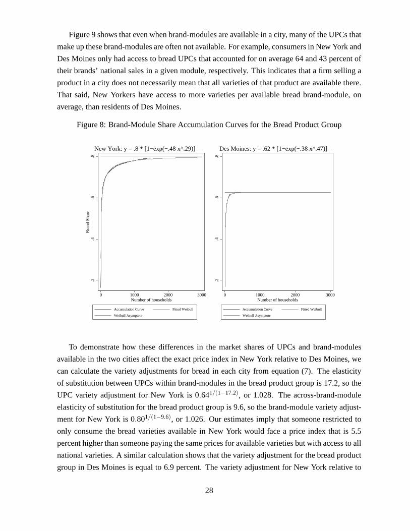
Figure 9 shows that even when brand-modules are available ina city, many of the UPCs that

make up these brand-modules are often not available. For example, consumers in New York and

Des Moines only had access to bread UPCs that accounted for onaverage 64 and 43 percent of

their brands’ national sales in a given module, respectively. This indicates that a firm selling a

product in a city does not necessarily mean that all varieties of that product are available there.

That said, New Yorkers have access to more varieties per available bread brand-module, on

average, than residents of Des Moines.

Figure 8: Brand-Module Share Accumulation Curves for the Bread Product Group

.2.4

.6.8

Bra

nd S

hare

0 1000 2000 3000Number of households

Accumulation Curve Fitted Weibull

Weibull Asymptote

New York: y = .8 * [1−exp(−.48 x^.29)]

.2.4

.6.8



Weibull Asymptote

Des Moines: y = .62 * [1−exp(−.38 x^.47)]

To demonstrate how these differences in the market shares ofUPCs and brand-modules

available in the two cities affect the exact price index in New York relative to Des Moines, we

can calculate the variety adjustments for bread in each cityfrom equation (7). The elasticity

of substitution between UPCs within brand-modules in the bread product group is 17.2, so the

UPC variety adjustment for New York is 0.641/(1−17.2), or 1.028. The across-brand-module

elasticity of substitution for the bread product group is 9.6, so the brand-module variety adjust-

ment for New York is 0.801/(1−9.6), or 1.026. Our estimates imply that someone restricted to

only consume the bread varieties available in New York wouldface a price index that is 5.5

percent higher than someone paying the same prices for available varieties but with access to all

national varieties. A similar calculation shows that the variety adjustment for the bread product

group in Des Moines is equal to 6.9 percent. The variety adjustment for New York relative to

28

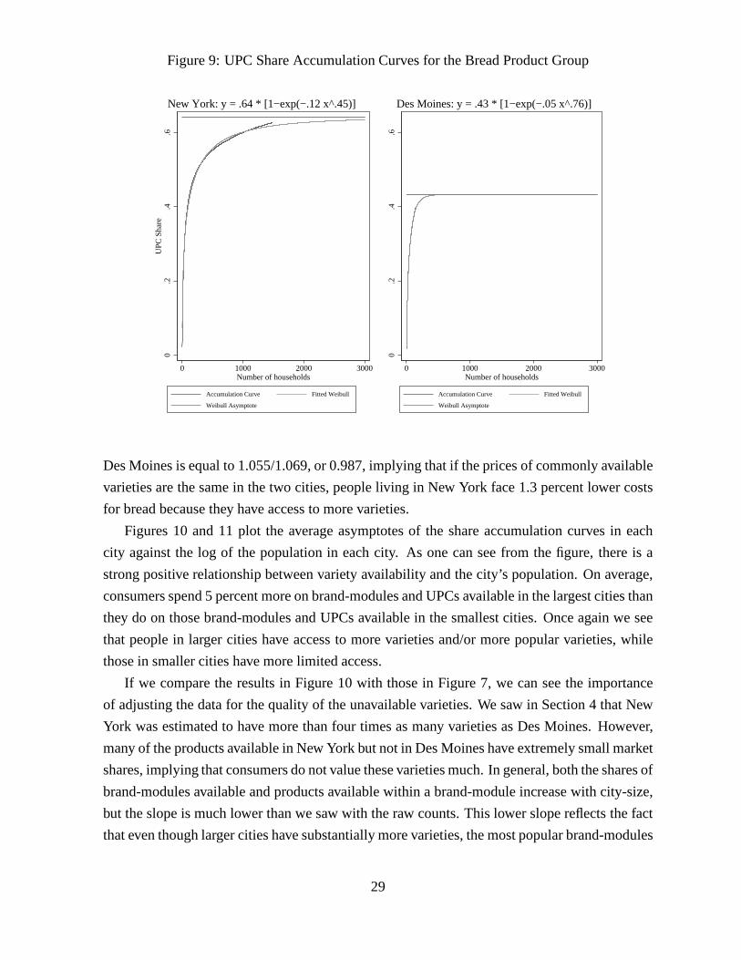
Figure 9: UPC Share Accumulation Curves for the Bread Product Group

0.2

.4.6

UP

C S

hare



Weibull Asymptote

New York: y = .64 * [1−exp(−.12 x^.45)]

0.2

.4.6



Weibull Asymptote

Des Moines: y = .43 * [1−exp(−.05 x^.76)]

Des Moines is equal to 1.055/1.069, or 0.987, implying that if the prices of commonly available

varieties are the same in the two cities, people living in NewYork face 1.3 percent lower costs

for bread because they have access to more varieties.

Figures 10 and 11 plot the average asymptotes of the share accumulation curves in each

city against the log of the population in each city. As one cansee from the figure, there is a

strong positive relationship between variety availability and the city’s population. On average,

consumers spend 5 percent more on brand-modules and UPCs available in the largest cities than

they do on those brand-modules and UPCs available in the smallest cities. Once again we see

that people in larger cities have access to more varieties and/or more popular varieties, while

those in smaller cities have more limited access.

If we compare the results in Figure 10 with those in Figure 7, we can see the importance

of adjusting the data for the quality of the unavailable varieties. We saw in Section 4 that New

York was estimated to have more than four times as many varieties as Des Moines. However,

many of the products available in New York but not in Des Moines have extremely small market

shares, implying that consumers do not value these varieties much. In general, both the shares of

brand-modules available and products available within a brand-module increase with city-size,

but the slope is much lower than we saw with the raw counts. This lower slope reflects the fact

that even though larger cities have substantially more varieties, the most popular brand-modules

29

Figure 10: Average Brand-Module Share Estimate vs. Log CityPopulation

DM

LR

Oma

SyrAlb

Bir

RicLou

GR

JacMemR−DNas

SLC

ChaCol

SA

Ind

OrlMil

NH

KC

Sac

NOOkCCin

Por

B−RPit

Tam

Den

StL

SD

Cle

Min

Pho

SeaMia

AtlHou

DalDet

Bos

Phi

SF

DC

Chi

LA

NY

.8.8

5.9

.95

Ave

rage

Bra

nd−

Sha

re


Average Brand Common Share Estimate Fitted values

Notes:

1. Common shares are averaged across product groups using national product group sales weights.


and products tend to be available everywhere.

The asymptotes of the share accumulation curves, in conjunction with our price data and

sales weights, enable us to estimate exact price indexes foreach city. Proposition 1 defines the

exact price index in terms of product group-specific conventional exact price indexes (CEPIgc)

and variety adjustments (VAgc). We aggregate across product groups to obtain values for each

of these components for each city. Rearranging terms in the exact price index definition from

Proposition 1, we can see that the exact price index is the product of each of these aggregate

components:

EPIc = ∏g∈G

[CEPIgcVAgc]wgc = ∏

g∈G

[CEPIgc]wgc ∏

g∈G

[VAgc]wgc =CEPIcVAc.

Table 5 presents our estimates for how the conventional exact price index (CEPIc), the variety

adjustment (VAc), and their product, the exact price index (EPIc), vary across cities. The first

three columns in the table use unadjusted prices to compute the index. As we saw in Table

2, unadjusted prices are higher in larger cities, and these results translate into a common exact

price index that rises with city size. These higher prices, however, are offset by an even stronger

30

Figure 11: Average UPC Share Estimate vs. Log City Population

DM

LR

Oma

SyrAlb

BirRicLou

GR

Jac

MemR−D

Nas

SLCChaCol

SA

Ind

Orl

Mil

NHKC

Sac

NO

OkC

Cin

Por

B−RPit

Tam

Den

StL

SD

CleMin

Pho

SeaMia

Atl

Hou

DalDet

Bos

Phi

SF

DC

ChiLA

NY.6

.65

.7.7

5.8

.85

Ave

rage

UP

C−

Sha

re


Average UPC Common Share Estimate Fitted values

Notes:

1. Common shares are averaged across product groups using national product group sales weights.


variety adjustment to prices arising from the greater availability of varieties in larger cities,

leading to an exact price index that falls slightly, but not significantly with city size.

Table 5: Are price indexes higher in larger cities?

Unadjusted PricesPrices Adjusted for Prices Adjusted for

Purchaser Heterogeneity Purchaser and Store Heterogeneity

CEPIc VAc EPIc CEPIc VAc EPIc CEPIc VAc EPIc

[1] [2] [3] [4] [5] [6] [7] [8] [9]Ln(Populationc) 0.012*** -0.016*** -0.0025 0.012*** -0.016*** -0.003 0.0041** -0.015*** -0.011***

[0.0035] [0.0028] [0.0050] [0.0034] [0.0028] [0.0050] [0.0018] [0.0028] [0.0036]Constant 0.82*** 1.31*** 1.11*** 0.82*** 1.31*** 1.12*** 0 .94*** 1.31*** 1.24***

[0.051] [0.042] [0.074] [0.050] [0.042] [0.073] [0.027] [0.042] [0.053]

Observations 49 49 49 49 49 49 49 49 49R-squared 0.206 0.394 0.005 0.201 0.394 0.007 0.096 0.388 0.167


Notes:1. The dependent variables in the above regressions are indices. These indices are calculated using unadjusted prices or prices that have beenadjusted as indicated above, using estimates from the regression in Column [4] of Panel A in Table 2.2. EPIc = CEPIcVAc which implies that log(EPIc) = log(CEPIc) + log(VAc). Note that the dependent variables in theabove regressions are in levels, not logs, so the coefficients on log population in the CEPIc and VAc regressions do not add to thecoefficient on log population in the EPIc regression.

31

Figure 12: City Price Indexes vs. Log City Population

Indexes Calculated using Unadjusted Prices

LROmaSyr BirRic

Lou

JacMem

R−D

Nas

SLC

Cha

Col

SA

Ind

Orl

Mil

NH

KC

Sac

OkCCin

Por

B−R

Pit

TamDen

StL

SD

Cle

Min

Pho

SeaMia

Atl

Hou

DalDet

BosPhi

SF

DCChi

LA NY

−.0

8−

.04

0.0

4.0

8ce

pi


LR

Oma

Syr

BirRic

Lou

JacMem

R−D

NasSLC

Cha

Col

SA

IndOrl

MilNH

KC

Sac

OkCCin

Por

B−R

Pit

Tam

DenStL

SD

Cle

Min

Pho

Sea

Mia

AtlHou

DalDetBosPhi

SF

DC

Chi

LA

NY

−.0

8−

.04

0.0

4.0

8ep

i


Indexes Calculated using PricesAdjusted for Purchaser and Store Heterogeneity

LR

OmaSyr

BirRic

LouJacMemR−DNas

SLC

ChaColSAIndOrlMilNHKC

Sac

OkCCinPorB−R

PitTamDenStL

SD

Cle

MinPho

SeaMia

AtlHou

Dal

Det

BosPhi

SF

DC

Chi

LA NY

−.0

8−

.04

0.0

4.0

8ce

pi


LR

Oma

Syr

BirRic

Lou

JacMem

R−D

Nas

SLC

ChaColSA

Ind

Orl

MilNHKCSac

OkCCin

Por

B−R

Pit

Tam

DenStL

SD

Cle

Min

Pho

Sea

MiaAtl HouDal

Det

BosPhi

SF

DC Chi

LA

NY

−.0

8−

.04

0.0

4.0

8ep

i


Notes:


2. City price indexes are normalized to be mean zero.

As we argued in Section 3.3, the unadjusted prices are problematic because they do not

correct for the store in which the goods are purchased or the type of household making the

purchase. We therefore use adjusted prices in the subsequent columns. Our price adjustments

are based on the estimates from Column 4 of Table 2. Adjustingfor purchaser heterogeneity

hardly has any impact in Table 2, and it barely affects our point estimates in Columns 4-6.

However, adjusting for retailer heterogeneity has a big impact. Columns 7-9 present results

in which we also control for retailer heterogeneity. We still obtain a statistically significant

positive association between city size and the common goodsprice index, but it is economically

small in size. On average, a person moving from a small city like Des Moines to New York City

would experience the price of commonly available groceriesrise by 1.6 percent. However, this

32

higher common goods price index would be more than offset by the fact that many goods are

not available and are therefore effectively priced at theirreservation level, resulting in the exact

price index in the small city being 4.2 percent higher.

We can assess the importance of the heterogeneity and variety availability biases visually in

Figure 12. The plots on the left shows how the common-goods exact price index varies across

cities, and the plots on the right shows how the exact price index varies. As we saw in Figure 2,

there is virtually no upward relationship between theCEPIc and population when we adjust for

heterogeneity biases and only a slight upward sloping relationship when we do not. Meanwhile,

the negative relationship between city population and the exact price index is robust and clearly

not driven by outliers.

Figure 12 also demonstrates how controlling for heterogeneity affects the variance of the

price level across cities. The common-goods exact price indexes plotted on the top left are

calculated with unadjusted prices. The variance of the price indexes that control for product

heterogeneity but not purchaser or store effects is 86 percent lower than the variance in our

replication of the ACCRA food price index. When we further control for purchaser and store

heterogeneity in the indexes on plotted on the bottom left, the variance falls by an additional 10

percentage points to just 3 percent of the variance of the ACCRA-style index. In sum, 97 percent

of the variance in urban price levels disappears when we movefrom anad hocprice index to

a theoretically-justified one that corrects for both heterogeneity and substitution biases. This

drop is almost identical to the 95 percent decline in variance that we observed comparing our

replication of the ACCRA food price index with the city fixed effects estimated in Section 5.3.

The methodological differences between the city fixed effects and the CES indexes, therefore,

play only a small role in the drop in variance. We attribute most of the variance in measured PPP

of commonly-available food products to heterogeneity biases, rather than substitution biases.31

It is also interesting to compare the common-good exact price index,CEPIc, in Table 5,

with the coefficient on the city fixed effects,αc, in Table 2. Recall that we can think of the

city fixed effects as a price index in the sense that they summarize the relative price levels

across locations, where relative prices are weighted by thetransaction-value weights used in

the regressions. An important difference between the two isthat the Sato-Vartia weights used

to calculate theCEPIc are theoretically justified if one assumes a CES utility function, whereas

the transaction weights used in the estimation of theαc’s do not have a theoretical justification

but rather serve an econometric purpose: to minimize the influence of errors associated with

small transactions on the estimates. Nevertheless, it is reassuring that the associations between

these variables and population are so close; the differences are typically around 0.002. This

indicates that our results regarding the computation of theprice level of available goods in a

city are robust to a number of sensible aggregation methods.

31These price indexes and their relative variances are listedin Appendix Table A.2.

33

Taken together with those in Section 3, these results suggest that conventional price indexes

provide a very misleading picture of what the prices of tradables are in cities and also help to

explain why. In Column 1 of Table 1, we saw that the elasticityof a conventional urban price

index with respect to population was 4.2 percent. However, once we controlled for product

heterogeneity, the fact that the standard urban price indexes don’t compare the same goods,

we see that the elasticity falls to 1.6 percent (Column 1 of Table 2): a loss of two-thirds of its

magnitude. Controlling for purchaser and especially retailer heterogeneity more than halves the

magnitude of this coefficient, taking it down to 0.6 percent.Further using the common exact

price index instead of anad hocone, which is the principle difference betweenCEPIc andαc,

reduces the coefficient to 0.4 percent (Column 7 of Table 5), which is less than one tenth of its

initial magnitude. Finally, the exact price index, which differs from theCEPIc by correcting

for variety availability (an extreme form of substitution bias), flips the sign, suggesting that the

elasticity of urban price with respect to population is -1.1percent (Column 9 of Table 5): a 5

percentage point differential. Thus, the standard result that the prices of tradables are higher in

cities is due to a series of measurement issues. If one uses a theoretically sound approach, the

result reverses.

5.4 Robustness

One possible concern about these results is that people who live in large cities might not shop

in all of the neighborhoods within the city’s borders. This might bias our variety adjustment

downwards because we may be counting varieties in, say, suburbs that are irrelevant for people

who live downtown.

An easy solution to this problem is to make use of the fact thatthe Nielsen data records the

household’s county and the zip codes of the stores in which they purchase each UPC. We first

assume that a household is located in the zip code in the county where its grocery expenditures

are the highest. We then construct the population of the market where households in each zip

code shop. For a set of households living in the same zip code,we sum the populations of

the zip codes where we observe the set of households purchasing UPCs. This sum tells us the

population of the market that is available to households located in that zip code. We average

these market populations across the zip codes in each city toyield the average population of

the neighborhoods where households in the city choose to shop. We refer to this number as the

relevant population.

Table 6 presents results in which we replace the city’s population with the relevant popu-

lation in the neighborhoods in which households actually shop. The results are, if anything,

stronger than the results using urban population as the measure of city size. The fact that the

results are so similar indicates that understanding where households shop within cities is not

34

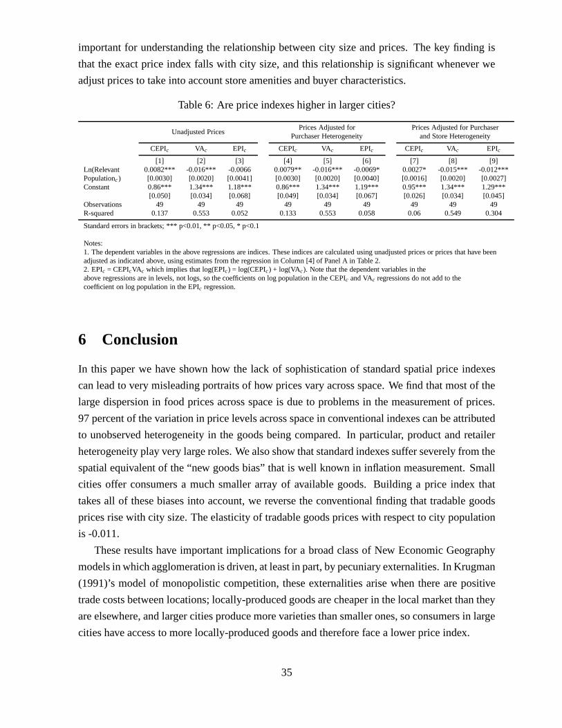
important for understanding the relationship between citysize and prices. The key finding is

that the exact price index falls with city size, and this relationship is significant whenever we

adjust prices to take into account store amenities and buyercharacteristics.

Table 6: Are price indexes higher in larger cities?

Unadjusted PricesPrices Adjusted for Prices Adjusted for Purchaser

Purchaser Heterogeneity and Store Heterogeneity

CEPIc VAc EPIc CEPIc VAc EPIc CEPIc VAc EPIc

[1] [2] [3] [4] [5] [6] [7] [8] [9]Ln(Relevant 0.0082*** -0.016*** -0.0066 0.0079** -0.016*** -0.0069* 0.0027* -0.015*** -0.012***Populationc) [0.0030] [0.0020] [0.0041] [0.0030] [0.0020] [0.0040] [0.0016] [0.0020] [0.0027]Constant 0.86*** 1.34*** 1.18*** 0.86*** 1.34*** 1.19*** 0 .95*** 1.34*** 1.29***

[0.050] [0.034] [0.068] [0.049] [0.034] [0.067] [0.026] [0.034] [0.045]Observations 49 49 49 49 49 49 49 49 49R-squared 0.137 0.553 0.052 0.133 0.553 0.058 0.06 0.549 0.304

Standard errors in brackets; *** p<0.01, ** p<0.05, * p<0.1

Notes:1. The dependent variables in the above regressions are indices. These indices are calculated using unadjusted prices or prices that have beenadjusted as indicated above, using estimates from the regression in Column [4] of Panel A in Table 2.2. EPIc = CEPIcVAc which implies that log(EPIc) = log(CEPIc) + log(VAc). Note that the dependent variables in theabove regressions are in levels, not logs, so the coefficients on log population in the CEPIc and VAc regressions do not add to thecoefficient on log population in the EPIc regression.

6 Conclusion

In this paper we have shown how the lack of sophistication of standard spatial price indexes

can lead to very misleading portraits of how prices vary across space. We find that most of the

large dispersion in food prices across space is due to problems in the measurement of prices.

97 percent of the variation in price levels across space in conventional indexes can be attributed

to unobserved heterogeneity in the goods being compared. Inparticular, product and retailer

heterogeneity play very large roles. We also show that standard indexes suffer severely from the

spatial equivalent of the “new goods bias” that is well knownin inflation measurement. Small

cities offer consumers a much smaller array of available goods. Building a price index that

takes all of these biases into account, we reverse the conventional finding that tradable goods

prices rise with city size. The elasticity of tradable goodsprices with respect to city population

is -0.011.

These results have important implications for a broad classof New Economic Geography

models in which agglomeration is driven, at least in part, bypecuniary externalities. In Krugman

(1991)’s model of monopolistic competition, these externalities arise when there are positive

trade costs between locations; locally-produced goods arecheaper in the local market than they

are elsewhere, and larger cities produce more varieties than smaller ones, so consumers in large

cities have access to more locally-produced goods and therefore face a lower price index.

35

More recent papers propose that other mechanisms are at playhere. Behrens and Robert-

Nicoud (2011) and Combes et al. (2012) demonstrate that, with quadratic linear preferences

and fixed trade costs as in Melitz and Ottaviano (2008), threerelated phenomena yield lower

prices in larger cities: (i) more efficient firms are more likely to locate in, or “select into,”

larger cities; (ii) firms in larger cities can take advantageof agglomeration economies in those

locations; and finally, (iii) larger cities are more competitive so firms charge lower markups

in these locations. Finally, Hummels et al. (2009) argue that scale economies in the shipping

industry lower costs and increase competition on routes to large markets. Similar economies in

domestic transportation could also lower prices in large cities.

While separating the contributions of each of these forces to understanding the spatial dis-

tribution of prices is beyond the scope of this paper, our results indicate that the New Economic

Geography framework is correct to predict that the price level of tradable goods tends to be

lower in larger cities.

36

References

Albouy, David, “The Unequal Geographic Burden of Federal Taxation,”Journal of Political

Economy, 2009,117(41), 635–667.

Aten, Bettina, “Report on Interarea Price Levels,”Bureau of Economic Analysis Working Pa-

pers, November 2005.

Atkin, David and Dave Donaldson, “Who’s Getting Globalized? The Size and Nature of

Intranational Trade Costs,”Yale University and MIT, unpublished mimeo, 2012.

B., Figueroa-E. Aten and T. Martin, “Notes on Estimating the Multi-Year Regional Price

Parities by 16 Expenditure Categories: 2005-2009,”Bureau of Economic Analysis Working

Papers, April 2012, (0071).

Behrens, Kristian and Frederic Robert-Nicoud, “Survival of the Fittest in Cities: Agglomer-

ation, Selection, and Inequality,”CEPR Discussion Papers, February 2011, (7019).

Bernard, Andrew B., J. Bradford Jensen, Stephen J. Redding,and Peter K. Schott, “Firms

in International Trade,”The Journal of Economic Perspectives, 2007,21 (3), pp. 105–130.

Broda, Christian and David E. Weinstein, “Understanding International Price Differences

Using Barcode Data,”NBER Working Paper No. 14017, 2008.

and , “Product Creation and Destruction: Evidence and Price Implications,” American

Economic Review, 2010,100, 691.

Burstein, Ariel and Gita Gopinath , “International Prices and Exchange Rates,”NBER Work-

ing Paper 18829, 2013.

and Nir Jaimovich, “Understanding Movements in Aggregate and Product-LevelReal Ex-

change Rates,”unpublished paper, UCLA and Stanford University, 2009.

Chevalier, Judith A., “Capital structure and product-market competition: Empirical evidence

from the supermarket industry,”The American Economic Review, 1995, p. 415–435.

Colwell, Robert K. and Jonathan A. Coddington, “Estimating Terrestrial Biodiversith

through Extrapolation,”Philosophical Transactions: Biological Sciences, July 1994,345

(1311), 101–118.

Combes, Pierre-Philippe, Gilles Duranton, Laurent Gobillon, Diego Puga, and Sébastien

Roux, “The productivity advantages of large cities: Distinguishing agglomeration from firm

selection,”Econometrica, 2012,80 (6), 2543–2594.

37

Couture, Victor , “Valuing the Consumption Benefits of Urban Density,” 2013.

Crucini, Mario J. and Mototsugu Shintani , “Persistence in law of one price deviations: Evi-

dence from micro-data,”Journal of Monetary Economics, 2008,55 (3), 629–644.

DuMond, J. Michael, Barry T. Hirsch, and David A. Macpherson, “Wage Differentials

Across Labor Markets and Workers: Does Cost of Living Matter?,” Economic Inquiry, Octo-

ber 1999,37 (4), 577–598.

Eaton, Jonathan, Samuel Kortum, and Francis Kramarz, “An anatomy of international

trade: Evidence from French firms,”Econometrica, 2011,79 (5), 1453–1498.

Ellickson, Paul B. and Sanjog Misra, “Supermarket pricing strategies,”Marketing Science,

2008,27 (5), 811–828.

Feenstra, Robert C., “New Product Varieties and the Measurement of International Prices,”

The American Economic Review, 1994,84 (1), 157–177.

and David E. Weinstein, “Globalization, Markups, and the U.S. Price Level,”NBER Work-

ing Paper 15749, Febraury 2010,35.

, Robert Inklaar, and Marcel Timmer , “The Next Generation of the Penn World Table,”

2012.

Fujita, Masahisa, “A Monopolistic Competition Model of Spatial Agglomeration,” Regional

Science and Urban Economics, 1988,18, 87–124.

Gopinath, Gita, Pierre-Olivier Gourinchas, Chang-Tai Hsieh, and Nicholas Li, “Interna-

tional prices, costs, and markup differences,”The American Economic Review, 2011,101(6),

2450–2486.

Handbury, Jessie, “Are Poor Cities Cheap for Everyone? Non-Homotheticity and the Cost of

Living Across U.S. Cities,” 2012.

and David E. Weinstein, “Goods Prices and Availability in Cities,”NBER Working Paper

17067, 2011.

Helpman, Elhanan, “The size of regions,” in Itzhak Zilcha David Pines, EfraimSadka, ed.,

Topics in Public Economics, Cambridge University Press, 1998, pp. 33–54.

Hummels, David and Peter J. Klenow, “The Variety and Quality of a Nation’s Exports,”The

American Economic Review, 2005,95 (3), 704–723.

38

, Volodymyr Lugovskyy, and Alexandre Skiba, “The trade reducing effects of market

power in international shipping,”Journal of Development Economics, 2009,89 (1), 84–97.

Jimenez-Valverde, Alberto, Silvia Jimenez Mendoza, Jose Martin Cano, and Miguel L.

Munguira , “Comparing relative model fit of several species-accumulation functions to local

Papilionoidea and Hesperioidea butterfly inventories of Mediterranean habitats,”Biodiversity

and Conservation, 2006,15, 163–176.

Krugman, Paul, “Increasing Returns and Economic Geography,”Journal of Political Econ-

omy, 1991,99 (3), 483–499.

Landry, Anthony , “Borders and Big Macs,”Economics Letters, 2013.

Mao, Chang Xuan, Robert K. Colwell, and Jing Chang, “Interpolating, Extrapolating, and

Comparing Incidence-Based Species Accumulation Curves,”Ecology, 2004,85(2717-2727),

433–441.

, , and , “Estimating the Species Accumulation Curve Using Mixtures,” Biometrics,

2005,61 (2), 433–441.

Melitz, Marc J. and Gianmarco I. P. Ottaviano, “Market Size, Trade, and Productivity,”

Review of Economic Studies, January 2008,75 (1), 295–316.

Moretti, Enrico , “Real Wage Inequality,”American Economic Journal: Applied Economics,

2013,5 (1), 65–103.

Ottaviano, Gianmarco I.P., Takatoshi Tabuchi, and Jacques-Francois Thisse, “Agglomera-

tion and Trade Revisited„”International Economic Review, May 2002,43 (2), 409–435.

Parsley, David C. and Shang-Jin Wei, “Convergence to the Law of One Price Without Trade

Barriers or Currency Fluctuations,”The Quarterly Journal of Economics, 1996, 111 (4),

1211–1236.

Rivera-Batiz, Francisco L., “Increasing Returns, Monopolistic Competition, and Agglomera-

tion Economies in Consumption and Production,”Regional Science and Urban Economics,

1988,18, 125–153.

Sato, Kazuo, “The Ideal Log-Change Index Number,”The Review of Economics and Statistics,

1976,58 (2), 223–228.

Schiff, Nathan, “Cities and product variety,”University of British Columbia, 2012.

39

Simonovska, Ina, “Income Differences and Prices of Tradables,”UC Davis Working Paper,

2010,No. 10-15.

Tabuchi, Takatoshi, “On Interregional Price Differentials,”The Japanese Economic Review,

March 2001,52 (1), 104–115.

Vartia, Y. , “Ideal Log-Change Index Numbers,”Scandinavian Journal of Statistics, 1976,3

(3), 121–126.

40

AppendicesTable A.1: Sample City Data

EffectiveSample Retail Normalized

Population1 Household Rent3 HerfindahlMarket Name (thousands) Count2 (psf) Index4

Correlation with Population 1.00 0.57 0.59 -0.30

Omaha (Oma) 717 116 11.70 0.116Jacksonville (Jac) 1,100 130 12.95 0.157Albany (Alb) 876 138 - 0.139San Diego (SD) 2,814 139 23.52 0.116Des Moines (DM) 456 145 - 0.176Syracuse (Syr) 732 164 10.77 0.078Milwaukee (Mil) 1,690 170 13.37 0.220Hartford-New Haven (NH) 1,725 193 14.53 0.138Richmond (Ric) 997 194 15.04 0.120Grand Rapids (GR) 1,089 198 - 0.221Kansas City (KC) 1,776 220 12.10 0.082Raleigh-Durham (R-D) 1,188 239 15.25 0.113Indianapolis (Ind) 1,607 245 12.82 0.109Orlando (Orl) 1,645 247 15.74 0.203Salt Lake City (SLC) 1,334 248 14.11 0.092Portland, Or (Por) 2,265 263 16.76 0.110Pittsburgh (Pit) 2,359 303 14.07 0.143Cincinnati (Cin) 1,979 317 12.52 0.201Memphis (Mem) 1,136 331 11.98 0.155Little Rock (LR) 584 351 11.11 0.193Cleveland (Cle) 2,946 362 13.88 0.095Nashville (Nas) 1,231 403 12.99 0.169New Orleans-Mobile (NO) 1,878 409 - 0.216Louisville (Lou) 1,026 454 13.46 0.209Oklahoma City-Tulsa (OkC) 1,887 528 9.83 0.147Birmingham (Bir) 921 570 12.81 0.154Dallas (Dal) 5,222 899 14.05 0.119San Antonio (SA) 1,592 921 12.48 0.305San Francisco (SF) 7,039 995 29.90 0.152Detroit (Det) 5,456 1,001 15.66 0.135Atlanta (Atl) 4,112 1,038 15.31 0.141Sacramento (Sac) 1,797 1,052 19.84 0.064Chicago (Chi) 9,158 1,064 16.92 0.127Houston (Hou) 4,670 1,070 13.63 0.143Miami (Mia) 3,876 1,086 20.08 0.286Columbus (Col) 1,540 1,101 10.97 0.171Charlotte (Cha) 1,499 1,115 14.89 0.132Washington, DC-Baltimore (DC) 7,608 1,115 21.49 0.070Denver (Den) 2,582 1,128 14.70 0.163Buffalo-Rochester (B-R) 2,268 1,135 11.20 0.176Seattle (Sea) 3,555 1,149 19.78 0.104Los Angeles (LA) 16,400 1,151 24.47 0.100Tampa (Tam) 2,396 1,173 13.11 0.198St. Louis (StL) 2,604 1,183 12.84 0.107Philadelphia (Phi) 6,188 1,183 17.02 0.066Phoenix (Pho) 3,252 1,211 16.27 0.129Minneapolis (Min) 2,969 1,236 14.99 0.165Boston (Bos) 5,819 1,275 19.03 0.122New York (NY) 21,200 1,477 20.13 0.088

Sources and notes:1. 2000 U.S. Census.2. 2005 Nielsen HomeScan sample.3. 2005 Community/Neighborhood Shopping Center EffectiveRents from reis.com.4. Herfindahl indexes measure the concentration of retail chains in each market.

41

Table A.2: Price Indexes

Price Indexes2

Nielsen Unadjusted Purchaser-Store AdjustedPopulation1 Food City Fixed City Fixed

Market Name (thousands) Index3 Effect4 CEPI6 Effect4 CEPI6 EPI6

Correlation with Population 1.00 0.49 0.44 0.43 0.42 0.37 -0.19Coefficient of Variation 6.8% 2.6% 2.2% 1.3% 1.1% 2.0%Var(Index)/Var(Nielsen Food Index) 0.18 0.13 0.05 0.03 0.12

Omaha (Oma) 717 0.802 0.959 0.968 0.963 0.971 1.039Jacksonville (Jac) 1,100 0.872 0.953 0.961 0.969 0.976 1.007Albany (Alb) 876 0.924 0.967 0.970 0.973 0.975 1.013San Diego (SD) 2,814 0.973 1.004 1.001 0.996 0.995 1.033Des Moines (DM) 456 0.844 0.927 0.940 0.964 0.974 1.039Syracuse (Syr) 732 0.847 0.953 0.961 0.967 0.972 1.014Milwaukee (Mil) 1,690 0.871 0.969 0.980 0.955 0.965 1.015Hartford-New Haven (NH) 1,725 0.976 0.998 0.998 0.987 0.9851.019Richmond (Ric) 997 0.849 0.954 0.963 0.976 0.983 1.007Grand Rapids (GR) 1,089 0.833 0.930 0.938 0.978 0.981 1.016Kansas City (KC) 1,776 0.840 0.953 0.962 0.975 0.980 1.014Raleigh-Durham (R-D) 1,188 0.905 0.972 0.981 0.968 0.977 1.003Indianapolis (Ind) 1,607 0.836 0.945 0.955 0.964 0.972 1.000Orlando (Orl) 1,645 0.907 0.961 0.970 0.971 0.975 0.985Salt Lake City (SLC) 1,334 0.818 0.928 0.936 0.948 0.957 0.976Portland, Or (Por) 2,265 0.834 0.963 0.964 0.978 0.979 1.022Pittsburgh (Pit) 2,359 0.827 0.973 0.982 0.977 0.982 1.008Cincinnati (Cin) 1,979 0.844 0.934 0.946 0.969 0.977 0.996Memphis (Mem) 1,136 0.813 0.946 0.960 0.976 0.987 1.016Little Rock (LR) 584 0.802 0.946 0.958 0.985 0.995 1.019Cleveland (Cle) 2,946 0.859 0.958 0.966 0.968 0.973 0.988Nashville (Nas) 1,231 0.806 0.934 0.947 0.965 0.976 0.992New Orleans-Mobile (NO) 1,878 0.877 0.952 0.965 0.980 0.9901.019Louisville (Lou) 1,026 0.827 0.927 0.938 0.964 0.973 0.993Oklahoma City-Tulsa (OkC) 1,887 0.830 0.937 0.950 0.964 0.973 0.996Birmingham (Bir) 921 0.858 0.948 0.961 0.971 0.982 1.002Dallas (Dal) 5,222 0.861 0.945 0.958 0.963 0.974 0.981San Antonio (SA) 1,592 0.784 0.909 0.923 0.953 0.964 0.982San Francisco (SF) 7,039 1.031 1.035 1.033 1.014 1.013 1.033Detroit (Det) 5,456 0.840 0.958 0.967 0.994 0.999 1.000Atlanta (Atl) 4,112 0.863 0.943 0.955 0.965 0.974 0.978Sacramento (Sac) 1,797 1.024 1.016 1.011 1.004 1.003 1.014Chicago (Chi) 9,158 0.902 0.968 0.974 0.961 0.966 0.970Houston (Hou) 4,670 0.798 0.925 0.941 0.955 0.966 0.976Miami (Mia) 3,876 0.932 0.981 0.990 0.980 0.986 0.979Columbus (Col) 1,540 0.835 0.941 0.952 0.974 0.980 0.988Charlotte (Cha) 1,499 0.885 0.985 0.996 0.969 0.978 0.984Washington, DC-Baltimore (DC) 7,608 0.911 0.965 0.969 0.975 0.978 0.972Denver (Den) 2,582 0.938 0.973 0.977 0.976 0.981 0.988Buffalo-Rochester (B-R) 2,268 0.859 0.941 0.953 0.965 0.973 0.993Seattle (Sea) 3,555 0.905 0.987 0.985 0.982 0.983 0.997Los Angeles (LA) 16,400 0.952 1.002 1.002 0.991 0.993 1.003Tampa (Tam) 2,396 0.905 0.963 0.972 0.972 0.976 0.963St. Louis (StL) 2,604 0.832 0.952 0.962 0.961 0.969 0.983Philadelphia (Phi) 6,188 0.938 0.968 0.971 0.984 0.986 0.979Phoenix (Pho) 3,252 0.857 0.968 0.971 0.969 0.972 0.941Minneapolis (Min) 2,969 0.900 0.971 0.983 0.969 0.981 0.998Boston (Bos) 5,819 0.937 0.965 0.972 0.977 0.983 0.980New York (NY) 21,200 1.000 1.000 1.000 1.000 1.000 1.000

Sources and notes:1. 2000 U.S. Census.2. All price indexes are relative to the price index for New York.3. Nieslen food index is replication of ACCRA food index, as described in Section 2.4. Unadjusted city fixed effects areαc estimates from equation (2) without purchaser demographicor storetype controls.5. Purchaser-store adjusted city fixed effects areαc estimates from equation (2) with purchaser demographic andstoretype controls.6. CEPI and EPI indexes are calculated according to methodology described in Section 5.

42

A Structural Variety Estimation

In Section 4, we used a non-structural “accumulation curve”methodology to estimate the num-

ber of UPCs available in each city. Here we demonstrate that astructural methodology yields

very similar results for how the number of varieties varies across cities.

A.1 Methodology

We first consider a simple case in which all UPCs are purchasedby households with the same

probability in order to develop the intuition, and then moveto a more realistic case in which

each UPC has its own purchase probability.

In order to work out the math in the simple case, assume that each household selects only one

UPC out of theSUPCs available in the market. If we also assume that each UPC is purchased

with a probabilityπ that is identical for all UPCs in the market, then it follows that π = 1/S.

Our task is to estimateS using the number of different UPCs purchased by a sample ofH

households. To do this, we make one additional assumption: stores have sufficient inventories

of goods so that the purchase of a UPC by one household does notreduce the probability of

another household buying the same UPC. If household purchases are independent in the cross-

section, then the probability that we observe one of theH households in our sample selecting

a particular UPC is equal to one minus the probability that none of theH households selects

the UPC, or 1− (1−1/S)H . The number of different UPCs that we expect to observe in the

purchase records of theH households is simply the sum of these probabilities across all of the

Savailable UPCs,

S(H) = S[1− (1−1/S)H] (A.1)

It is immediately apparent that equation (A.1) is an accumulation curve that has been derived

from a particular set of assumptions. It would be straightforward to obtain an estimate for the

number of varieties in the market in this simple case. By equating S(H) to the sample UPC

count,S(H), we can derive an estimate for the number of available UPCs that satisfies equation

(A.1). Note that the accumulation curve,S(H) should follow the negative exponential function

(which a special case of one of the functional forms we considered in Section 4:

S(H) = S(

1−e− ln((1−1/S)H))

(A.2)

This simple approach cannot be applied to the data for two reasons. First, households pur-

chase more than one UPC in the course of a year. And second, some UPCs, like milk, are likely

to be purchased at higher frequencies than other UPCs, like salt. Hence the probability that we

observe the purchase of a UPC will vary across UPCs. We can deal with the first problem by

43

allowing the purchase probability,π , to differ from 1/S. The second problem, however, is more

complicated because solving it requires us to know the purchase frequencies not only of every

observed UPC but also of the UPCs that we do not observe in our sample. In order to solve this

problem, we follow Mao et al. (2005).

We allow for different products to have different purchase probabilities, but we restrict these

probabilities to be identical for groups of UPCs that we willrefer to as “incidence groups.”

This is not that restrictive an assumption, as we do not put a limit on the number of incidence

groups but only assume that some UPCs from each incidence group are purchased in our data.

Grouping UPCs in this way enables us to estimate the purchasefrequencies for all of the UPCs

in an incidence group even though we may only observe a fraction of the UPCs in the group

being purchased.

To put this concretely, suppose that each UPCu has a probability ofπcu of being selected

by a household in cityc, and that there areK different incidence groups, or values thatπcu

can take in each cityc, such thatπcu = πck for each UPC in incidence groupk. We defineαck

as the proportion of UPCs in incidence groupk in city c, i.e., the proportion of UPCs that are

selected with probabilityπck in city c. For example, when residents of a particular city choose

to purchase a good, the probability that they will purchase any given UPC can take one ofK

values. The incidence groups do not map directly into the product groups or product modules.

The estimated purchase frequency associated with each UPC within a product group or brand-

module will vary with the popularity of the UPC, which may be correlated with its brand,

container, size, and other characteristics. The UPCs in thehigh frequency incidence group tend

to be the most popular varieties of products that are frequently purchased,e.g. 12-packs of

some soda varieties, which are purchased by almost a third ofthe households in our sample.

Less popular varieties of soda tend to fall into the lower purchase frequency incidence groups,

along with the UPCs in less frequently purchased product categories,e.g.,cake yeast.

Suppose that there areSc UPCs available in cityc. If we again assume that household

purchases are independent in the cross-section, we can express the probability that any of the

UPCs in incidence groupk available in cityc is purchased by one ofHc households as one minus

the probability that none of theHc households selects the UPC, or 1− (1−πck)Hc. Taking the

weighted average of these probabilities across incidence groups (using incidence group shares

as weights), we can now express the unconditional probability that any one UPC available in

city c is observed in the purchases of a sample ofHc householdswithout knowing its incidence

groupasK

∑k=1

αck(1− (1−πck)Hc). The number of different UPCs that we expect to observe in

the purchase records ofHc households in cityc is the sum of these probabilities across all of the

44

Sc available UPCs, or

Sc(Hc) = Sc

K

∑k=1

αck(1− (1−πck)Hc). (A.3)

Mao et al. (2004) note that equation (A.3) can be re-written as:

Sc(Hc) = Sc

K

∑k=1

αck(1−exp(CckHc)) whereCck =− ln(1−πck)

Equation (A.3) is therefore referred to as the “generalizednegative exponential” (GNE) model.

It is straightforward to see that equation (A.2) is a specificcase of equation (A.3) in which the

selection probability is identical for all UPCs,i.e., K = 1 andπ = 1/S. Moreover, if we knew

the share of all goods in each incidence group,αck, and the probability that each UPC was

purchased,πck, (A.3) would just give us the equation of a particular accumulation curve for a

city.

Fortunately, we can use maximum likelihood estimation to estimateSc as well as theαck

andπck for any choice ofK. The number of households purchasing productu in city c, hcu,

follows a binomial distribution where the probability of observinghcu purchases is given by:

P(hcu) = ϕ(hcu;πcu) =

(

Hc

hcu

)

(πcu)hcu(1−πcu)

(Hc−hcu) (A.4)

whereHc is the total number of households in the sample for cityc,

(

Hc

hcu

)

≡Hc!

hcu!(Hc−hcu)!

and once againπcu = πci for each UPC,u, in categoryk. Let {hcu}u∈Ucbe the observed counts

of each UPC purchased by our sample of households in a cityc, whereUc is the set of UPCs

observed in the cityc sample. Now, we can define the binomial mixture distributionas follows:

Φ(hcu) =K

∑k=1

αckϕ(hcu;πck)

This distribution tells us the unconditional probability of observinghcu purchases ofanyUPCu

in our data, regardless of its incidence group, given the size and purchase probabilities of each

of the incidence groups.

Mao et al. (2005) derive a maximum likelihood methodology for estimating theα ’s andπ ’s

for a givenK using data on the number of samples (in our case, households)in which each

variety is observed. The variablenc j is defined to be the number of products that are purchased

45

by j households in the dataset for cityc, i.e., for which hcu equals j. In other words, if 100

UPCs are purchased by no households, 50 UPCs are purchased by1 household, and 25 UPCs

are purchased by 2 households, then we would havenc0 = 100; nc1 = 50; andnc2 = 25. The

joint likelihood of the total number of products available in the city and the parameters of the

mixture distribution is

L(

Sc,{αck,πck}Kk=1

)

=Sc!

Hc

∏j=0

nc j!

Hc

∏j=0

Φ( j)nc j

Note that from equation (A.3), we know that the number of available products,Sc, is a func-

tion of the number of observed products,Sc(Hc) =Hc

∑j=1

nc j, and the parameters of the mixture

distribution,{αck,πck}Kk=1. Therefore, we only need to estimate the parameters of the mixture

distribution to derive an estimate for the number of available products. To do so, we will max-

imize a conditional likelihood function. Letϕ(hcu;πcu) be a zero-truncated binomial density,

i.e., the probability that a product is purchased byj households conditional on it being pur-

chased by more than one household, andΦ ( j) =K∑

k=1αckϕ ( j;πck) be the mixture distribution

over these densities forK incidence groups. If we denote the total number of UPCs that are

purchased by at least one household in the samplenc+, the conditional likelihood function is

L(

Sc,{αck,πck}Kk=1

)

=nc+!

Hc

∏j=1

nc j!

Hc

∏j=1

Φ( j)nc j (A.5)

Equation (A.5) gives us the likelihood function as a function of the number of incidence

groups,K. In order to identify the correct number of these groups, we estimate the parameters

of mixture distributions for a range of values forK using the conditional likelihood function.

Each distribution implies a different estimate for the total number of UPCs available in a city.

We then compute the Akaike Information Criterion (AIC) for each value ofK in each city. We

choose between the distributions by selecting the number ofincidence groups for all cities equal

to theK that maximizes the sum of the AICs across all cities. The intuition for this procedure is

that each additional incidence group improves the fit but adds parameters, and the AIC provides

a way of determining how many groups are likely to exist in thedata.32

Once we have our estimates for theα ’s andπ ’s, we can use equation (A.3) to obtain an

32We also assume that the sampling is sufficient so that we observe some UPCs purchased in each incidencegroup. We need this assumption because we cannot say anything about the number of goods in an incidence groupthat are purchased with such low a probability that no one in the sample ever buys them. In other words, we canonly discuss the number of available varieties for observable classes of goods.

46

estimate of the total number of varieties as follows:

Sc = Sc(Hc)

[

K

∑k=1

αck(1− (1− πck)Hc)

]−1

(A.6)

where variables with circumflexes represent parameter estimates andSc(Hc) is equal to the

sample count of distinct varieties in the city. It is useful to note that when the number of

sampled households in the city,Hc approaches infinity, the fact that theα ’s sum to one implies

that our count of the number of distinct products purchased by these households becomes our

estimate of the number of varieties.

A.2 Results

With 49 cities, the GNE approach involves the estimation of several hundred parameters, so we

do not report all the values here. The AIC indicates that UPCstend to fall within 10 incidence

groups in terms of their purchase frequency. Table A.3 summarizes these estimates across our

sample of 49 cities. We see that in all cities there are few UPCs that are purchased with very

high frequency—on average, one in ten thousand UPCs are purchased with a frequency of 0.5

by a household. This would correspond to about 8 UPCs in the typical city having a purchase

probability of 0.5 over the course of a year by a typical household. However, we also see

that the vast majority of UPCs have extremely low purchase probability. 49 percent of UPCs

have a purchase probability of approximately one in a thousand. Thus, the product space is

characterized by a few UPCs with high purchase probabilities and a vast number of UPCs that

are rarely purchased.

Table A.3: Summary Statistics for GNE Parameter Estimates

Incidence Group (k)Probability of Purchase (πc,k) Share of UPCs (αc,k)Mean Standard Deviation Mean Standard Deviation

1 0.496 0.096 0.00009 0.000062 0.332 0.103 0.00041 0.000293 0.226 0.085 0.00116 0.000714 0.152 0.066 0.00300 0.001815 0.102 0.052 0.00757 0.004706 0.065 0.035 0.01953 0.010457 0.038 0.022 0.05083 0.018218 0.019 0.011 0.12115 0.018799 0.008 0.004 0.30803 0.0327710 0.001 0.001 0.48823 0.03465

Another way of summarizing the estimates is to examine how the probability that a UPC

47

is purchased varies with city size. We would expect that the probability that any consumer

purchases any one UPC would go down as the range of available UPCs in the city increases.

Fortunately, this is easy to examine given that our GNE structure enables us to estimate the

average probability that a household in cityc purchases a UPC by simply calculating

Πc =K

∑k=1

αc,kπc,k.

In Figure A.1, we see that the estimated average probabilityof purchase (which uses no popu-

lation data in its estimation) decreases sharply with city size. A UPC sold in our smallest city,

Des Moines, has three times the probability of being purchased by any individual household as a

UPC sold in New York. The fact that households in larger cities are much less likely to buy any

individual UPC is strongly suggestive of the fact that that the parametric estimate of the UPCs

available in a city is increasing with city size. We test thisdirectly by using the GNE parameter

Figure A.1: Average Purchase Probability vs. Log City Population

DM

LR

Oma

Syr

Alb

Bir

RicLou

GRJac

MemR−DNas

SLC

ChaColSA

Ind

Orl

Mil

NHKC

Sac

NOOkC

CinPor

B−R

Pit

TamDenStL

SD

Cle

MinPhoSeaMiaAtl

HouDalDet

BosPhi

SFDC

ChiLA

NY

0.0

05.0

1.0

15A

vera

ge P

urch

ase

Pro

babi

lity


Average Purchase Probability Fitted values

Notes:

1. Average purchase probability is the average of the estimated probability of a household purchasing a UPC in each incidence group

weighted by the estimated share of UPCs in the same incidencegroup,i.e., Average Purchase Probability in Cityc= Πc = ∑10k=1 αc,kπc,k.


estimates to calculate an estimate for total number of varieties in each city and considering how

this varies with city size. Figure A.2 plots how the log estimated number of varieties in each city

varies with city size. The results in Table A.4 shows that therelative relationship between the

estimated number of varieties and city size using the GNE is almost identical to that obtained

with the Weibull. The first three columns repeat the regression results reported in Columns 4

through 6 of Table 4. The last three columns repeat these regressions with the log GNE asymp-

48

tote instead of the log Weibull asymptote as the dependent variable. The coefficients on log

population are almost identical in all three specifications.33

Table A.4: Do larger cities have more UPC varieties?

Ln(Weibull Asymptote) Ln(GNE Asymptote)

[1] [2] [3] [4] [5] [6]Ln(Populationc) 0.278*** 0.300*** 0.261*** 0.281*** 0.303*** 0.275***

[0.0364] [0.0572] [0.0821] [0.0340] [0.0534] [0.0769]Ln(Per Capita Incomec) - -0.137 -0.060 - -0.129 -0.074

- [0.288] [0.312] - [0.269] [0.292]Income Herfindahl Index - -0.630 -0.178 - -0.321 0.000

- [2.641] [2.745] - [2.466] [2.568]Race Herfindahl Index - 0.074 0.109 - 0.111 0.135

- [0.347] [0.353] - [0.324] [0.330]Birthplace Herfindahl Index - -0.012 0.004 - -0.028 -0.017

- [0.238] [0.241] - [0.222] [0.225]Ln(Land Areac) - - 0.060 - - 0.042

- - [0.0898] - - [0.0840]Constant 6.912*** 8.057*** 7.240** 6.937*** 7.962*** 7.381**

[0.533] [2.860] [3.132] [0.498] [2.670] [2.930]Observations 49 49 49 49 49 49R-squared 0.55 0.56 0.56 0.59 0.60 0.60


Figure A.2: Log GNE Estimate vs. Log City Population

DM

LR

Oma

Syr Alb

Bir

Ric

Lou

GR

Jac

MemR−D

Nas

SLC

ChaCol

SA

IndOrl

Mil

NHKC

Sac

NOOkCCin

Por

B−R

Pit

TamDenStL

SD

Cle

MinPhoSeaMia

AtlHouDal

DetBos

Phi

SF

DC

ChiLA

NY

1010

.511

11.5

Ln(G

NE

Var

iety

Est

imat

e)


Ln(GNE Variety Estimate) Fitted values

Notes:


33This is not surprising, given that the correlation between the Weibull and GNE asymptotes, or variety esti-mates, is 0.99.

49

B Formulas for Sato-Vartia Weights

wuc =

shuc−shulnshuc−lnshu

∑b′∈Bg

∑u′∈Ub′

(

shu′c−shu′

lnshu′c−lnshu′

) , wbc =

shbc−shblnshbc−lnshb

∑b′∈Bg

(

shb′c−shb′

lnshb′c−lnshb′

) andwgc =

shgc−shglnshgc−lnshg

∑g′∈G

(

shg′c−shg′

lnshg′c−lnshg′

)

shuc, shbc, andshgc are city-specific expenditure shares defined as follows:

shuc=vuc

∑b′∈Bg

∑u′∈Ub′

vu′c, shbc=

∑u∈Ub

vuc

∑b′∈Bg

∑u′∈Ub′

vu′candshgc=

∑b∈Bg

∑u∈Ub

vuc

∑g′∈G

∑b′∈Bg′

∑u′∈Ub′

vu′c

shu, shb, andshg are national expenditure shares defined as follows:

shu =vu

∑b′∈Bg

∑u′∈Ub′

vu′, shb =

∑u∈Ub

vu

∑b′∈Bg

∑u′∈Ub′

vu′andshg =

∑b∈Bg

∑u∈Ub

vu

∑g′∈G

∑b′∈Bg′

∑u′∈Ub′

vu′

for vu = ∑cvuc. G denotes set of product groups, andGc denotes the set of product groups with

products sold in cityc. Mathematically,Gc = {g∈ G|Bg 6= /0}. All product groups are sold in

every city, soGc = G.

50

Goods Prices and Availability in Cities

Documents

Transcript of Goods Prices and Availability in Cities