Goodness-of-fit tests for a heavy taileddistribution

Alex J. Koning∗ Liang Peng†

Econometric Institute Report 2005-44

Abstract

For testing whether a distribution function is heavy tailed, we study theKolmogorov test, Berk-Jones test, score test and their integrated versions. Acomparison is conducted via Bahadur efficiency and simulations.

The score test and the integrated score test show the best performance.Although the Berk-Jones test is more powerful than the Kolmogorov-Smirnovtest, this does not hold true for their integrated versions; this differs from re-sults in Einmahl and McKeague (2003), which shows the difference of Berk-Jones test in testing distributions and tails.Keywords. Bahadur efficiency, heavy tail, tail index.

Contents

1 Introduction 2

2 Methodologies 42.1 The KS, BJ and SC supremum tests . . . . . . . . . . . . . . . . 42.2 Bahadur efficiency . . . . . . . . . . . . . . . . . . . . . . . . . 62.3 The KSI, BJI and SCI quadratic tests . . . . . . . . . . . . . . . . 8

3 Simulation study and real applications 93.1 Simulation study . . . . . . . . . . . . . . . . . . . . . . . . . . 93.2 Real applications. . . . . . . . . . . . . . . . . . . . . . . . . . . 10

4 Proofs 11∗Econometric Institute, Erasmus University Rotterdam. Email: koning@few.eur.nl†School of Mathematics, Georgia Institute of Technology, Atlanta GA 30332-0160, USA.

Email: peng@math.gatech.edu

1

1 INTRODUCTION 2

1 Introduction

We say that a distribution has a heavy tail with tail index if

limt→∞

1− F (tx)

1− F (t)= x−α for all x > 0 (1.1)

holds for some α > 0 (notation: 1 − F ∈ RVα). Heavy tailed distributions havebeen applied in many different areas such as population size (Zipf (1949)), randomgraph (Reittu and Norros (2004)), internet traffic (Resnick (1997a)), hydrology(Katz et al. (2002)), finance (Danielsson and de Vries (1997)).

Most of the theoretical work on heavy tailed distributions concentrates on es-timating the tail index α. One of the best known estimators is the Hill estimator

α =

k−1

k∑

j=1

log Xn,n−k+j − log Xn,n−k

−1

(1.2)

(Hill (1975)), which employs a fraction of upper order statistics Xn,n−k, Xn,n−k+1,. . . , Xn,n. Several data-driven methods for choosing the sample fraction k/nare proposed in the literature; see Drees and Kaufmann (1998), Danielsson et al.(2001) and Guillou and Hall (2001).

As far as we know, goodness-of-fit testing has not received as much attentionas tail index estimation. An interesting aspect of testing goodness-of-fit of theheavy tail distribution is that the null hypothesis provides a description of theheavy tail distribution which is incomplete in the following two aspects:

(i) The tail index is unknown under the null hypothesis, and hence should beestimated. It is well-known that estimation of unknown parameters hasan non-neglible effect on the distribution of the test statistics, see Durbin(1973a,b).

(ii) The tail index only describes the tail behaviour of the heavy tail distribution,and thus only gives a partial description of the underlying distribution.

By fitting a generalized Pareto distribution to exceedances over a high thresh-old, Davison and Smith (1990) employed Kolmogorov and Anderson-Darling sta-tistics to test the fit, and compared these statistics to 5% critical values for testingan exponential distribution with unknown mean. However, using these critical val-ues in this context “is suspect since the exponential distribution is only a submodelof the generalized Pareto distribution, so the true critical points are smaller”, seeDavison and Smith (1990, p. 414).

1 INTRODUCTION 3

In Choulakian and Stephens (2001) critical values for Cramer-von Mises andAnderson-Darling statistics for testing a generalized Pareto distribution with un-known shape parameter are given.

If X has a generalized Pareto distribution with unknown shape parameter,then ln X has an exponential distribution with unknown mean, and thus tests ofexponentiality may be used to test the generalized Pareto distribution, see Marohn(2002).

Recently, Drees et al. (2004) employed the Cramer-von Mises statistic to testthe null hypothesis that a distribution is in the domain of attraction with ex-treme value index larger than −1/2. This may be thought as a generalizationof Choulakian and Stephens (2001), since a deterministic threshold is replaced bya random threshold in Drees et al. (2004)).

As far as the present authors know, no work has been done on comparingthe performance of goodness-of-fit tests for heavy tailed distributions under thealternative hypothesis. In this paper we compare three tests, the Kolmogorov test,the Berk-Jones test and the “estimated score” test.

The Kolmogorov test, Kolmogorov (1933); Smirnov (1948); Durbin (1973a),has a long tradition in statistics, and thus is an obvious choice as long as there areno other tests which clearly perform better.

The Berk-Jones test, Berk and Jones (1978, 1979), may be viewed as a non-parametric likelihood test, and was derived for the situation where the null hy-pothesis completely specifies the distribution of the observations. In this partic-ular situation, the Berk-Jones test was shown to be more efficient, in the senseof Bahadur efficiency, than any weighted Kolmogorov test at any alternative. InLi (2003) it is argued that the Berk-Jones test should also perform better thanthe Kolmogorov test in situations where the null hypothesis does not completelyspecify the distribution of the observations.

In contrast to the Berk-Jones test, the “estimated score” test in Hjort and Koning(2002) was specifically proposed for the situation where parameters are unknown.

We organize this paper as follows. In section 2 we present Kolmogorov test,Berk-Jones test, score test and their integrated versions. Large deviations resultsfor tail empirical processes are obtained as a byproduct of studying Bahadur effi-ciency. A simulation study and real applications are given in section 3. All proofsare put in section 4.

2 METHODOLOGIES 4

2 Methodologies

2.1 The KS, BJ and SC supremum tests

In order to motivate our methods, we shall first restrict ourselves to the quintessen-tial example of a heavy tailed distribution, the Pareto distribution. The Paretodistribution is defined by

G(x; α, β) = 1− (x/β)−α for all x > β (2.1)

where α > 0 is a shape parameter, and β > 0 is a scale parameter. For conve-nience, let G(x; α) denote G(x; α, 1) = 1− x−α.

Let Xn,1 ≤ Xn,2 ≤ · · · ≤ Xn,n denote an ordered sample of size n drawn fromthe Pareto distribution with unknown shape and scale parameters α and β. Choose1 ≤ k ≤ n. Let Rk,j denote Xn,n−k+j/Xn,n−k for j ≤ k, and note that Rk,1 ≤Rk,2 ≤ · · · ≤ Rk,k. One may show that the random variables Rk,1, Rk,2, . . . , Rk,k

are jointly equal in distribution to an ordered sample of size k drawn from thePareto distribution with shape parameter α and scale parameter 1.

Let Fk(r) denote the empirical distribution function of Rk,1, Rk,2, . . . , Rk,k,defined by

Fk(r) = k−1

k∑

j=1

I(Rk,j ≤ r).

Observe that for r > 1

1− Fk(r) =1

k

n∑

i=1

I(Xi > rXn,n−k).

The Kolmogorov test is based on the statistic supr>1 |KS(r; α)|, where

KS(r; α) = 1− Fk(r)− 1−G(r; α) = 1− Fk(r)− r−α,

and α =

k−1∑k

j=1 log Rk,j

−1

is the Hill estimator.

The Berk-Jones test is based on the statistic supr>1 kBJ(r; α), where

BJ(r; α) = 2K (Fk(r), G(r; α)) = 2K(

Fk(r), 1− r−α)

,

and the function K is defined by

K (p, p) = p lnp

p+ (1− p) ln

1− p

1− p. (2.2)

2 METHODOLOGIES 5

The estimated score test is based on the statistic supr>1 |SC(r; α)|, where

SC(r; α) = Fk(r)−∫ r

1

(1− Fk(s)) dΛ(s; α) = Fk(r)− α

∫ r

1

1− Fk(s)

sds,

and Λ(r; α) = − ln (1−G(r; α)) = α ln r is the cumulative hazard functionbelonging to G(r; α) defined by (2.1).

Suppose that X1, · · · , Xn are i.i.d. observations with distribution function F .We intend to test whether F has a heavy tailed distribution, see (1.1). Let U(x)denote the inverse function of 1/(1 − F (x)). Then (1.1) implies U ∈ RV1/α.In order to study the limiting behaviors of KS(r; α), BJ(r; α) and SC(r; α), wefurther assume that there exists a function A(t) → 0, as t →∞, such that

limt→∞

U(tx)/U(t) − x1/α

A(t)= x1/α xρ − 1

ρ(2.3)

for all x > 0, where ρ ≤ 0; see de Haan and Stadtmuller (1996) for details. Ourfirst result is as follows.

Theorem 1. Suppose F satisfies (2.3) and k = k(n) →∞, k/n → 0,√

kA(n/k) →0 as n →∞. Then

supx>1

∣

∣

∣

√kKS(x; α)

∣

∣

∣

d→ sup0<x<1

∣

∣

∣

∣

W (x)− xW (1) + x log(x)

∫ 1

0

W (s)− sW (1)

sds

∣

∣

∣

∣

and

supx>1

∣

∣

∣

√kSC(x; α)

∣

∣

∣

d→ sup0<x<1

∣

∣

∣

∣

W (x)− xW (1)−∫ x

0

W (s)− sW (1)

sds + x

∫ 1

0

W (s)− sW (1)

sds

∣

∣

∣

∣

,

where W (x) is a Wiener process.

Remark 1. For any fixed x−1/α ∈ (0, 1), we can show by Taylor expansions that

BJ(x−1/α; α)d→ W (x)− xW (1) + x log(x)

∫ 1

0W (s)−sW (1)

sds2

x(1− x)

and

EW (x)− xW (1) + x log(x)

∫ 1

0W (s)−sW (1)

sds2

x(1− x)=

x(1− x)− x2log(x)2

x(1− x),

2 METHODOLOGIES 6

i.e., the expectation of the limiting of BJ(x; α) depends on location x. This isdifferent from Berk & Jones test for testing distribution functions. But it may stillbe interesting to find the limiting distribution of an supx>1 BJ(x; α)−bn for somenormalizing constants an > 0 and bn. When F (x) = exp−x−α, we have

1

k

n∑

i=1

I(Xi > y−1/αXn,n−k)

d=

1

k

k∑

i=1

I(−α logU(Yn,n−i+1)

U(Yn,n−k)< log y)

=1

k

k∑

i=1

I(loglog(1− Y −1

n,n−i+1)

log(1− Y −1n,n−k)

< log y),

where Y ′n,is are defined in the proof of Theorem 1 below. That is, the distributions

of

supx>1

∣

∣

∣

√kKS(x; α)

∣

∣

∣, sup

x>1BS(x; α) and sup

x>1

∣

∣

∣

√kSC(x; α)

∣

∣

∣

are independent of α when F (x) = exp−x−α. This property is employed tosimulate critical values from test statistics themselves; see Section 3 for details.

2.2 Bahadur efficiency

It is known that when the null hypothesis is simple, that is, completely specifiesthe distribution of the observations, the Berk-Jones test is more efficient, in Ba-hadurs sense, than any weighted KolmogorovSmirnov test at any alternative, seeBerk and Jones (1978, 1979).

Extending this result to the situation where the null hypothesis is composite,that is, does not completely specify the distribution of the observations, requireshard work, which is typically avoided. Instead, it is argued that “one may ex-pect similar optimal properties for our test for the composite hypothesis”, see forinstance Li (2003, p. 178).

In this subsection, we adopt a similar approach. That is, we study the Bahadurefficiency of the “simple null hypothesis tests” based on statistics

supr>1

kBJ(r; α0) and supr>1

∣

∣

∣

√kKS(r; α0)

∣

∣

∣

rather than the Bahadur efficiency of “composite null hypothesis tests” based onthe statistics

supr>1

kBJ(r; α) and supr>1

|√

kKS(r; α)|.

2 METHODOLOGIES 7

First we state the definition of exact slope of a test statistic. Let (S,A) be thesample space of infinitely many independent and identically distributed observa-tions s = (X1, X2, · · · ) on an abstract random variable X . Let Pθ : θ ∈ Ωbe a collection of probability distributions of X , where Ω is a parameter space,and let Ω0 be a proper subset of Ω. Consider the hypothesis H0 : θ ∈ Ω0. LetTn(X1, · · · , Xn) be a sequence of test statistics. Assume that there exists anFn(t) such that

Pθ(Tn ≤ t) = Fn(t) (2.4)

for all θ ∈ Ω0 and all t ∈ R. Then the level obtained by Tn is defined to be

Ln(X1, · · · , Xn) = 1− Fn(Tn(X1, · · · , Xn)).

If

limn→∞

n−1 log Ln(X1, · · · , Xn) = −1

2c(θ) a.s.Pθ, (2.5)

then we say the sequence Tn has exact slope c(θ) when θ obtains.The following proposition describes a useful method of finding the exact slope

of a given sequence Tn for which (2.4) holds; see Bahadur (1971) for a detailedproof.

Proposition 1. Suppose that

limn→∞

n−1/2Tn(X1, · · · , Xn) = b(θ) a.s.Pθ

for each θ ∈ Ω1 = Ω \ Ω0, where −∞ < b(θ) < ∞, and that

limn→∞

n−1 log1− Fn(n1/2t) = −f(t)

for each t in an open interval A, where f is a continuous function on A, andb(θ) : θ ∈ Ω1 ⊂ A. Then (2.5) holds with c(θ) = 2f(b(θ)) for each θ ∈ Ω1.

Now we are ready to give our results on Bahadur efficiency. Let Ω0 = F :1 − F ∈ RVα0

, Ω1 = F : 1 − F ∈ RVα, α > 0, α 6= α0 and Ω = Ω0 ∪ Ω1,where α0 > 0 is given. Then we have the following result.

Theorem 2. Suppose k = k(n) → ∞, k/n → 0 and k/ log log n → ∞ asn →∞. Then

limn→∞

supr>1

|KS(r; α0)| = |(α0

α)− α

α0−α − (α0

α)−

α0α0−α | a.s. (2.6)

for each F ∈ Ω1 and that, for a ∈ (0, 1),

limn→∞

k−1 log PΩ0sup

r>1|KS(r; α0)| ≥ a = −f(a), (2.7)

2 METHODOLOGIES 8

where f(a) = inff1(a, t) : 0 ≤ t ≤ 1 and

f1(a, t) =

(a + t) log a+tt

+ (1− a− t) log 1−a−t1−t

for 0 ≤ t ≤ 1− a,

∞ for t > 1− a.

Remark 2. Using the same arguments as in Berk and Jones (1979), we concludeby Theorem 2 that supx>1 |kBJ(r; α0)| is more Bahadur efficient than supr>1

|√

kKS(r; α0)| for testing H0 : F ∈ Ω0 against Ha : F ∈ Ω1.

Remark 3. It would be interesting to show that (2.6) holds for a larger Ω1. Ifwe replace supr>1 |

√kKS(r; α0)| by supr>b |

√kKS(r; α0)|, where b > 1 is given,

then Ω1 includes all distributions F such that limt→∞ supx>b1−F (tx)1−F (t)

= 0. In thiscase, the left hand side of (2.6) becomes supx>b x−α0 = b−α0 .

2.3 The KSI, BJI and SCI quadratic tests

The KS, BJ and SC tests introduced in paragraph 2.1 are supremum tests, whichare based on statistics obtained by taking the supremum over some underlyinggoodness-of-fit process. Quadratic tests are popular alternatives to supremumtests, and are based on statistics obtained by integrating the squared goodness-of-fit process with respect to some appropriate measure. In this subsection weconsider “quadratic” variants of the KS, BJ and SC tests.

The Cramer-von Mises test statistic KSI is defined by

KSI =

∫ ∞

1

√

kKS(r; α)2 dG(r; α)

As in Einmahl and McKeague (2003), see also Wellner and Koltchinskii (2003),define the integrated BJ test statistic BJI by

BJI =

∫ ∞

1

kBJ(r; α) dG(r; α)

Finally, define the integrated score test SCI by

SCI =

∫ ∞

1

√

kSC(r; α)2 dG(r; α).

The following theorem gives the limiting distributions of these three test statistics.

Theorem 3. Suppose F satisfies (2.3) and k = k(n) →∞, k/n → 0,√

kA(n/k) →0 as n →∞. Then

KSId→

∫ 1

0

W (x)− xW (1) + x log(x)

∫ 1

0

W (s)− sW (1)

sds2 dx, (2.8)

3 SIMULATION STUDY AND REAL APPLICATIONS 9

BJId→

∫ 1

0

W (x)− xW (1) + x log(x)∫ 1

0W (s)−sW (1)

sds2

x(1− x)dx (2.9)

and

SCId→

∫ 1

0

W (x)−xW (1)−∫ x

0

W (s)− sW (1)

sds+x

∫ 1

0

W (s)− sW (1)

sds2 dx,

(2.10)where W (x) and α are defined in Theorem 1.

3 Simulation study and real applications

3.1 Simulation study

First we simulate 100,000 random samples from Frechet distribution F (x) =exp−x−1 with sample size n = 1000, and then compute the test statistics KS =supr>1 |

√kKS(r; α)|, BJ = supr>1 kBJ(r; α), SC = supr>1 |

√kSC(r; α)|, KSI,

BJI and SCI for k = 20, 30, · · · , 200. Based on these computed test statistics, weobtain the 0.95 level critical values; see Table 1.

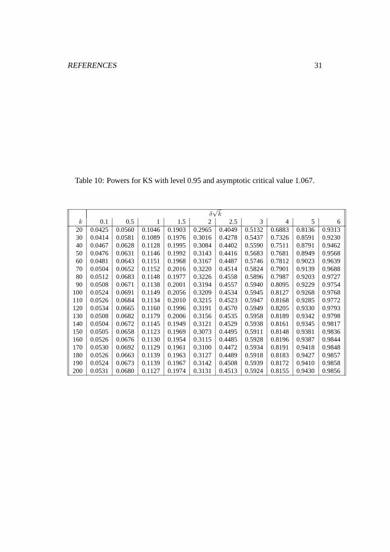
Using Table 1, we compute the powers of these six test statistics by simu-lating 10,000 random samples from distributions 1 − F (x) = 1 + α log x

δ−1 −δ−1

,(x > 1), with sample size n = 1000, α = 1, k = 20, 30, · · · , 200 and δ

√k =

0.1, 0.5, · · · , 6; see Tables 2–7. Since the limiting distribution of BJ does not exist,we compare the other five tests by simulating critical values from their correspond-ing limiting distributions. More specifically, we first simulated 100,000 randomsamples of Wiener Processes on [0, 1] with 1000 equally spaced grid points, andthen compute the limitings of the test statistics. The critical values with level 0.95are 1.338, 0.456, 1.076, 0.220 and 1.313 for SC, SCI, KS, KSI and BJI, respec-tively. Using these numbers, we compute the powers of those five tests as above,which are reported in Tables 8–12.

We summarize our observations from Tables 2–12 as follows:

1. When the exact critical values are employed, the SCI test is most powerfulfor most values of k and δ. And the BJ test is more powerful than the KStest, which coincides with the Bahadur efficiency study in section 2.

2. When the asymptotic critical values are employed, the SCI test is still mostpowerful for most values of k and δ. But the BJI test is less powerful than theKSI test. This seems contradicting Einmahl and McKeague (2003), wherean integrated empirical likelihood test is more powerful than the Cramer-von Mises test. Note that the Berk-Jones test is an empirical likelihood

3 SIMULATION STUDY AND REAL APPLICATIONS 10

test when testing distributions. Since the limiting of kBJ(r; α) is not a chi-squared distribution (see Remark 1), the BJI test is not an exact integratedempirical likelihood test. This is a difference of Berk-Jones test in testingdistribution and tails.

3. The tests with asymptotic critical values are comparable to the correspond-ing tests with exact critical values when k is small, but are more powerfulwhen k is large. This may be because the asymptotic critical values areobtained from the limiting without taking the bias, introduced by a large k,into account.

3.2 Real applications.

The first data set we analyzed consists of 2156 Danish fire loss over one millionDanish krone from the years 1980 to 1990 inclusive (see Figure 1). The lossfigure is a total loss for the event concerned and includes damage to buildings,furnishings and personal property as well as loss of profits. This Danish fire lossdata set was analyzed by McNeil (1997) and Resnick (1997b), where the right tailindex was confirmed to be between 1 and 2. Here we apply the five tests SC, SCI,KS, KSI and BJI to test whether this data set has a heavy tailed distribution. Thecritical values obtained from the limiting distributions were employed to computethe test statistics for k = 20, 21, · · · , 2000 by step 1; see Figure 2. The Hillestimators are plotted against k in Figure 2 as well. For a large range of k, all testsdo not reject the heavy tailed hypothesis. However, there is a bit strange patternaround k = 150.

Ideally, when the heavy tailed hypothesis is true, tests should not reject thenull hypothesis for small values of k, and reject it for large values of k sincethe critical values are obtained by ignoring the bias. Moreover there should beone region where decision varies due to the fact that the bias and variance arecomparable in this range of k. We suspect that this strange pattern in Figure 2may be due to weak dependence inside the danish fire loss data. Next, we usethe first 2150 data points and divide into 215 blocks with 10 points in each block.Then we apply those five tests to the maxima in these blocks, see Figure 3. Thisfigure clear shows the ideal pattern. So, it would be very interesting to investigatehow the bias, i.e., lim

√kA(n/k) 6= 0, affects the tests and to propose tests for

heavy tailed time series.The second data set we analyzed is the internet traffic data. The Ethernet se-

ries used here are part of a data set collected at Bellcore in August of 1989. Theycorrespond to one ”normal” hour’s worth of traffic, collected every 10 millisec-onds, thus resulting in a length of 360,000. This data set measures the number ofbytes per unit time; see Figure 4. This data set was first analyzed in Leland et al.

4 PROOFS 11

(1994). We apply those five tests to this data set, which clearly reject the heavytailed hypothesis; see Figure 5. Next we divide this data set into 600 blocks with600 points in each block, and apply those five tests the maxima in each blocks;see Figure 6. Figure 6 still rejects the heavy tailed hypothesis. This may be dueto the long-range dependence of the internet traffic data. How to test heavy taildistributions for long-range dependent data is quite interesting both theoreticallyand practically since there exist debates on fitting a heavy tailed distribution orlog-normal distribution to internet traffic data.

4 Proofs

Proof of Theorem 1. Let Y1, · · · , Yn be i.i.d. random variables with distribution1− y−1, (y > 1), and Yn,1 ≤ · · · ≤ Yn,n denote the order statistics of Y1, · · · , Yn.Then, it follows from de Haan and Resnick (1998) that

√k1

k

n∑

i=1

I(Yi >n

kx)− x d→ W (x),

√kk

nYn,n−[kx] − x−1 d→ x−2W (x),

√k1

k

n∑

i=1

I(Xi > xXn,n−k)− x−α d→ W (x−α)− x−αW (1),

√kα− α d→ −α2

∫ ∞

1

s−1W (s−α) ds + αW (1) (4.1)

in D[1,∞), where W (x) is a Wiener process. So

√kKS(x; α)

=√

k1

k

n∑

i=1

I(Xi > xXn,n−k)− x−α

+√

kx−α − x−αd→ W (x−α)− x−αW (1)− x−α log xα2

∫ ∞

1

s−1W (s−α) ds− αW (1)(4.2)

in D[1,∞). Hence

supx>1

|√

kKS(x; α)| d→ sup0<x<1

|W (x)− xW (1) + x log(x)

∫ 1

0

W (s)− sW (1)

sds|.

4 PROOFS 12

Similarly, we have√

kSC(x; α)

= −√

k1

k

n∑

i=1

I(Xi > xXn,n−k)− x−α

−α

∫ x

1

s−1√

k1

k

n∑

i=1

I(Xi > xXn,n−k)− s−α ds

−√

kα− α

αx−α − 1

d→ −W (x−α) + x−αW (1) + α

∫ ∞

x

W (s−α)− s−αW (1)

sds

−αx−α

∫ ∞

1

W (s−α − s−αW (1)

sds (4.3)

in D[1,∞). Hence

supx>1

|√

kSC(x; α)|

d→ sup0<x<1

|W (x)− xW (1)−∫ x

0

W (s)− sW (1)

sds + x

∫ 1

0

W (s)− sW (1)

sds|.

Before we prove theorem 2, we give the following Lemma on large deviationsfor tail processes, which may be of independent interest. Note that Cheng (1992)gave large deviations results for Hill’s estimator.Lemma 1. Under the condition of Theorem 2, we have, for 0 < a < 1,

k−1 log PΩ0(sup

x>1KS(x; α0) ≥ a) → −f(a),

k−1 log PΩ0(sup

x>1−KS(x; α0) ≥ a) → −f(a)

andk−1 log PΩ0

(supx>1

|KS(x; α0)| ≥ a) → −f(a).

Proof. Here we only show the first limit. The other two can be shown in a similarway as proving the first limit and Example 5.3 of Bahadur (1971). Let U1, · · · , Un

be i.i.d. random variables with uniform distribution on [0, 1] and Un,1 ≤ · · · ≤Un,n denote the order statistics of U1, · · · , Un. Put Gn,k+1(u) = P (Un,k+1 ≤ u).By Potters’ inequality (see Geluk and de Haan (1987)), for any ε > 0, there existsu0 > 0 such that, for all 0 < u ≤ u0 and 0 < s ≤ 1,

(1− ε)s−1/α0+ε ≤ (1− F )−(us)/(1− F )−(u) ≤ (1 + ε)s−1/α0−ε. (4.4)

4 PROOFS 13

Write

PΩ0(sup

x>1KS(x; α0) ≥ a)

= PΩ0(sup

x>11

k

k∑

i=1

I((1− F )−(Un,i)

(1− F )−(Un,k+1)> x)− x−α0 ≥ a)

=

∫ u0

0

PΩ0(sup

x>11

k

k∑

i=1

I((1− F )−(Un,i)

(1− F )−(u)> x)− x−α0 ≥ a|Un,k+1 = u) dGn,k+1(u)

+

∫ 1

u0

PΩ0(sup

x>11

k

k∑

i=1

I((1− F )−(Un,i)

(1− F )−(u)> x)− x−α0 ≥ a|Un,k+1 = u) dGn,k+1(u)

= I1 + I2. (4.5)

Let V1, · · · , Vk be i.i.d. random variables with uniform distribution on [0, 1]. Itfollows from (4.4) that, for any x > 1 and ε ∈ (0, 1),

I1 ≥∫ u0

0

PΩ0(1

k

k∑

i=1

I((1− F )−(Un,i)

(1− F )−(u)> x)− x−α0 ≥ a|Un,k+1 = u) dGn,k+1(u)

≥∫ u0

0

PΩ0(1

k

k∑

i=1

I((1− ε)(Un,i

u)−1/α0+ε > x)− x−α0 ≥ a|Un,k+1 = u) dGn,k+1(u)

≥∫ u0

0

PΩ0(1

k

k∑

i=1

I(Un,i

u< (

x

1− ε)−

α01−α0ε )− x−α0 − a ≥ 0|Un,k+1 = u) dGn,k+1(u)

=

∫ u0

0

PΩ0(1

k

k∑

i=1

I(Vi < (x

1− ε)−

α01−α0ε )− x−α0 − a ≥ 0) dGn,k+1(u).

By Theorem 3.1 of Bahadur (1971),

lim infn→∞

k−1 log(I1)

≥ lim infn→∞

k−1 log PΩ0(1

k

k∑

i=1

I(Vi < (x

1− ε)−

α01−α0ε )− x−α0 − a ≥ 0)

+ lim infn→∞

k−1 log Gn,k+1(u0)

≥ −f1(x−α0 − x

−α0

1−α0ε + a, (x

1 + ε)−

α01−α0ε ) + lim inf

n→∞k−1 log Gn,k+1(u0).

Let ε → 0 and take infinimum over x > 1, we get

lim infn→∞

k−1 log(I1) ≥ −f(a) + lim infn→∞

k−1 log Gn,k+1(u0).

4 PROOFS 14

Since Un,k+1p→ 0, i.e., Gn,k+1(u0) → 1, we have

lim infn→∞

k−1 log PΩ0(sup

x>1KS(x; α0) ≥ a) ≥ lim inf

n→∞k−1 log(I1) ≥ −f(a). (4.6)

For any positive integer m, define ∆(m) = inf (j−1)α0−jα0

mα0: j = 1, · · · , m.

Then ∆(m) → 0 as m →∞. Since

supm/j≤x≤m/(j−1)

1

k

k∑

i=1

I((1− F )−(Un,i)

(1− F )−(u)> x)− x−α0

≤ 1

k

k∑

i=1

I((1− F )−(Un,i)

(1− F )−(u)>

m

j)− (

m

j − 1)−α0

for j = 1, · · · , m, we have, for 0 < u ≤ u0

P (supx>1

1

k

k∑

i=1

I((1− F )−(Un,i)

(1− F )−(u)> x)− x−α0 ≥ a|Un,k+1 = u)

≤m

∑

j=1

P (1

k

k∑

i=1

I((1− F )−(Un,i)

(1− F )−(u)>

m

j)− (

m

j − 1)−α0 ≥ a|Un,k+1 = u)

≤m

∑

j=1

P (1

k

k∑

i=1

I(Un,i

u< (

m

j(1 + ε))−

α01+α0ε )− (

m

j − 1)−α0 − a ≥ 0|Un,k+1 = u)

=m

∑

j=1

P (1

k

k∑

i=1

I(Vi < (m

j(1 + ε))−

α01+α0ε )− (

m

j − 1)−α0 − a ≥ 0).

Choose m large enough such that 0 < ( mj−1

)−α0 − ( mj(1+ε)

)−

α01+α0ε < 1 for all

0 < ε < 1 and j = 1, · · · , m. By Theorem 2.1 of Bahadur (1971), we have

P (1

k

k∑

i=1

I(Vi < (m

j(1 + ε))−

α01+α0ε )− (

m

j − 1)−α0 − a ≥ 0)

≤ exp−kf1((m

j − 1)−α0 − (

m

j(1 + ε))−

α01+α0ε + a, (

m

j(1 + ε))−

α01+α0ε ),

i.e.,

P (supx>1

1

k

k∑

i=1

I((1− F )−(Un,i)

(1− F )−(u)> x)− x−α0 ≥ a|Un,k+1 = u)

≤m

∑

j=1

exp−kf1((m

j − 1)−α0 − (

m

j(1 + ε))−

α01+α0ε + a, (

m

j(1 + ε))−

α01+α0ε ).

4 PROOFS 15

Letting ε → 0, we obtain that

P (supx>1

1

k

k∑

i=1

I((1− F )−(Un,i)

(1− F )−(u)> x)− x−α0 ≥ a|Un,k+1 = u)

≤m

∑

j=1

exp−kf1((m

j − 1)−α0 − (

m

j)−α0 + a, (

m

j)−α0)

≤ m exp−kf1(a + ∆(m), (m

j)−α0)

≤ m exp−kf(a + ∆(m)),

i.e.,I1 ≤ m exp−kf(a + ∆(m)). (4.7)

By Hoeffding’s inequality (Hoeffding (1963)) we have

P (Un,k+1 > u0)

= P (

n∑

i=1

I(Ui > u0) ≥ n− k − 1)

≤ exp−2n(u0 −k + 1

n)2.

Hence

lim supn→∞

1

kP (Un,k+1 > u0)m

−1 expkf(a + ∆(m)) = 0,

i.e,

lim supn→∞

k−1 log(1 + I2/I1) ≤ lim supn→∞

k−1 log1 + (1−Gn,k+1(u0))/I1 = 0.

(4.8)By (4.7) and (4.8),

lim supn→∞

k−1 log PΩ0(sup

x>1KS(x; α0) ≥ a) ≤ −f(a). (4.9)

Hence, it follows from (4.6) and (4.9) that

limn→∞

k−1 log PΩ0(sup

x>1KS(x; α0) ≥ a) = −f(a).

Proof of Theorem 2. (2.6) follows from the fact that

limn→∞

supx>1

|KS(x; α0)| = supx>1

|x−α − x−α0 | a.s.

for F ∈ Ω1, and (2.7) follows from Lemma 1.

4 PROOFS 16

Proof of Theorem 3. Obviously, (2.8) and (2.10) follow from (4.2) and (4.3), re-spectively. To prove (2.9), we follow the lines of Einmahl and McKeague (2003).For ε ∈ (0, 1), write

−∫ ∞

1

BJ(x; α) dx−α

=

∫ ε

0

BJ(x−1/α; α) dx +

∫ 1−ε

ε

BJ(x−1/α; α) dx +

∫ 1

1−ε

BJ(x−1/α; α) dx

= I1 + I2 + I3.

By (4.1), (4.2) and Taylor expansions, we can show that

I2d→

∫ 1−ε

ε

W (x)− xW (1) + x log(x)∫ 1

0W (s)−sW (1)

sds2

x(1− x)dx (4.10)

for any ε ∈ (0, 1). Thus, we only need to show that, as n →∞,

I1 = Op(√

ε) and I3 = Op(√

ε) (4.11)

uniformly in ε ∈ (0, 1/2). Put ∆n(x) = 1k

∑ni=1 I(Xi > xXn,n−k). Write I1 as

II1 + · · ·+ II7, where

II1 = −∫ ε∧(

Xn,n

Xn,n−k)−α

0

k log(1− x) dx

II2 = −∫ ε

ε∧(Xn,n

Xn,n−k)−α

I(x ≥ ∆n(x−1/α))2k1−∆n(x−1/α)

×log(1 +x−∆n(x−1/α)

1− x)− x−∆n(x−1/α)

1− x dx,

II3 =

∫ ε

ε∧(Xn,n

Xn,n−k)−αn

I(x < ∆n(x−1/α))2k1−∆n(x−1/α)

×log(1 +∆n(x−1/α)− x

1−∆n(x−1/α))− ∆n(x−1/αn)− x

1−∆n(x−1/α) dx,

II4 =

∫ ε

ε∧(Xn,n

Xn,n−k)−α

I(x ≥ ∆n(x−1/α))2k∆n(x−1/α)

×log(1 +x−∆n(x−1/α)

∆n(x−1/α))− x−∆n(x−1/α)

∆n(x−1/α) dx,

4 PROOFS 17

II5 = −∫ ε

ε∧(Xn,n

Xn,n−k)−α

I(x < ∆n(x−1/α))2k∆n(x−1/α)

×log(1 +∆n(x−1/α)− x

x)− ∆n(x−1/α)− x

x dx,

II6 = −∫ ε

ε∧(Xn,n

Xn,n−k)−α

I(x ≥ ∆n(x−1/α)2k(x−∆n(x−1/α))2

1− xdx,

II7 = −∫ ε

ε∧(Xn,n

Xn,n−k)−α

I(x < ∆n(x−1/α))2k(∆n(x−1/α)− x)2

xdx.

Let U1, · · · , Un be i.i.d. random variables with uniform distribution on [0, 1], andUn,1 ≤ · · · ≤ Un,n denote the order statistics. It follows from Einmahl (1997) thatthere exists a sequence of Wiener processes Wn such that for any δ > 0

supt>0

t−1/2e−δ| log t||√

k1

k

n∑

i=1

I(Ui ≤k

nt)− t −Wn(t)| p→ 0 (4.12)

as n → ∞, where k = k(n) → ∞ and k/n → 0 as n → ∞. Using (4.12) andsimilar arguments in Drees et al. (2004), we can show that, for any δ > 0,

sup0<x≤ 1

2

x−1/2+δ|√

k∆n(x−1/α)− x −Wn(x) + xWn(1)

+x log(x)

∫ 1

0

Wn(s)− sWn(1)

sds−

√kA(n/k)αx

x−ρ − 1

ρ| p→ 0(4.13)

as n →∞. Note that

| log(1 + y)− y| ≤ 2y2 for y ≥ 0. (4.14)

It is easy to check that for any δ1 > 0 and δ2 > 0

P (k−1−δ1 ≤ (Xn,n

Xn,n−k

)−α ≤ k−1+δ2) → 1 (4.15)

and

P (k−1−δ1 ≤ 1− (Xn,n−k+1

Xn,n−k

)−α ≤ k−1+δ2) → 1 (4.16)

as n →∞. By (4.15), we have

II1 = Op(√

ε) uniformly in ε ∈ (0, 1/2).

REFERENCES 18

Using (4.13), (4.14) and (4.15), we have

|II5| ≤∫ ε

ε∧(Xn,n

Xn,n−k)−α

4k1−∆n(x−1/α)x−∆n(x−1/α)

x2 dx

=

∫ ε

ε∧(Xn,n

Xn,n−k)−α

4k(∆n(x−1/α)− x)3

x2dx

+

∫ ε

ε∧(Xn,n

Xn,n−k)−α

4k(∆n(x−1/α)− x)2

xdx

= Op(I(ε > k−1−δ1)

∫ ε

0

1√k

(x1/2−δ)3

x2dx)

+Op(

∫ ε

0

(x1/2−δ)2

xdx) uniformly in ε ∈ (0, 1/2)

= Op(√

ε) uniformly in ε ∈ (0, 1/2).

Similarly, we can show that

IIi = Op(√

ε) uniformly in ε ∈ (0, 1/2)

for i = 2, 3, 4, 6, 7. Hence

I1 = Op(√

ε) uniformly in ε ∈ (0, 1/2).

Similarly, we can show that

I3 = Op(√

ε) uniformly in ε ∈ (0, 1/2).

Thus, the theorem follows.

Acknowledgment. Peng’s research was partly supported by NSF grant DMS0403443.Alex J. Koning is grateful to the School of Mathematics at the Georgia Instituteof Technology for hospitality and financial support.

References

R. R. Bahadur. Some limit theorems in statistics. Society for Industrial and Ap-plied Mathematics, Philadelphia, Pa., 1971.

Robert H. Berk and Douglas H. Jones. Relatively optimal combinations of teststatistics. Scandinavian Journal of Statistics, 5(3):158–162, 1978.

REFERENCES 19

Robert H. Berk and Douglas H. Jones. Goodness-of-fit test statistics that domi-nate the Kolmogorov statistics. Zeitschrift fur Wahrscheinlichkeitstheorie undVerwandte Gebiete, 47(1):47–59, 1979.

Shi Hong Cheng. Large deviation theorem for Hill’s estimator. Acta MathematicaSinica. New Series, 8(3):243–254, 1992.

V. Choulakian and M. A. Stephens. Goodness-of-fit tests for the generalizedPareto distribution. Technometrics, 43(4):478–484, 2001.

J. Danielsson and C. G. de Vries. Tail index and quantile estimation with very highfrequency data. Journal of Empirical Finance, 4(2-3):241–257, June 1997.

J. Danielsson, L. de Haan, L. Peng, and C. G. de Vries. Using a bootstrap methodto choose the sample fraction in tail index estimation. Journal of MultivariateAnalysis, 76(2):226–248, 2001. doi: 10.1006/jmva.2000.1903.

A. C. Davison and R. L. Smith. Models for exceedances over high thresholds.Journal of the Royal Statistical Society. Series B. Methodological, 52(3):393–442, 1990.

Laurens de Haan and Sidney Resnick. On asymptotic normality of the Hill esti-mator. Communications in Statistics. Stochastic Models, 14(4):849–866, 1998.

Laurens de Haan and Ulrich Stadtmuller. Generalized regular variation of secondorder. Australian Mathematical Society. Journal. Series A. Pure Mathematicsand Statistics, 61(3):381–395, 1996.

Holger Drees and Edgar Kaufmann. Selecting the optimal sample fraction in uni-variate extreme value estimation. Stochastic Processes and their Applications,75(2):149–172, 1998.

Holger Drees, Laurens de Haan, and Deyuan Li. Approxima-tions to the tail empirical distribution function with applicationto testing extreme value conditions. Technical Report 2004-01, Fachbereich Mathematik, Universitat Hamburg, 2004. URLhttp://www.math.uni-hamburg.de/meta/preprints/ims/prst2004-01.html.

J. Durbin. Distribution theory for tests based on the sample distribution function.Society for Industrial and Applied Mathematics, pages vi+64, Philadelphia, Pa.1973a.

James Durbin. Weak convergence of the sample distribution function when para-meters are estimated. The Annals of Statistics, 1:279–290, 1973b.

REFERENCES 20

John H. J. Einmahl. Poisson and Gaussian approximation of weighted local em-pirical processes. Stochastic Processes and their Applications, 70(1):31–58,1997. doi: 10.1016/S0304-4149(97)00055-0.

John H. J. Einmahl and Ian W. McKeague. Empirical likelihood based hypothesistesting. Bernoulli, 9(2):267–290, 2003.

J. L. Geluk and L. de Haan. Regular variation, extensions and Tauberian theo-rems, volume 40 of CWI Tract. Stichting Mathematisch Centrum - Centrumvoor Wiskunde en Informatica, Amsterdam, 1987. ISBN 90-6196-324-9.

Armelle Guillou and Peter Hall. A diagnostic for selecting the threshold in ex-treme value analysis. Journal of the Royal Statistical Society. Series B. Statisti-cal Methodology, 63(2):293–305, 2001. doi: 10.1111/1467-9868.00286.

Bruce M. Hill. A simple general approach to inference about the tail of a distrib-ution. The Annals of Statistics, 3(5):1163–1174, 1975.

Nils Lid Hjort and Alexander Koning. Tests for constancy of model parametersover time. Journal of Nonparametric Statistics, 14(1-2):113–132, 2002. doi:10.1080/10485250211394. Statistical models and methods for discontinuousphenomena (Oslo, 1998).

Wassily Hoeffding. Probability inequalities for sums of bounded random vari-ables. J. Amer. Statist. Assoc., 58:13–30, 1963.

Richard W. Katz, Marc B. Parlange, and Phillipe Naveau. Statistics of extremesin hydrology. Advances in Water Resources, 25:12871304, 2002. doi: 10.1016/S0309-1708(02)00056-8.

A.N. Kolmogorov. Sulla determinazione empirica di una legge di distribuzione.Giorn. Ist. Ital. Attuari., 4:83–91, 1933.

W. E. Leland, M. S. Taqqu, W. Willinger, and D. V. Wilson. On the self-similarnature of ethernet traffic (extended version). IEEE/ACM Transactions on Net-working, 2:1–15, Feb 1994.

Gang Li. Nonparametric likelihood ratio goodness-of-fit tests for survivaldata. Journal of Multivariate Analysis, 86(1):166–182, 2003. doi: 10.1016/S0047-259X(02)00058-1.

Frank Marohn. A characterization of generalized Pareto distributions by progres-sive censoring schemes and goodness-of-fit tests. Communications in Statistics.Theory and Methods, 31(7):1055–1065, 2002. doi: 10.1081/STA-120004902.

REFERENCES 21

Alexander J. McNeil. Estimating the tails of loss severity distributions using ex-treme value theory. Astin Bulletin, 27(1):117–137, 1997.

Hannu Reittu and Ilkka Norros. On the power-law random graph model of massivedata networks. Performance Evaluation, 55(1-2):3–23, Jan 2004. doi: 10.1016/S0166-5316(03)00097-X.

Sidney I. Resnick. Heavy tail modeling and teletraffic data. The Annals of Statis-tics, 25(5):1805–1869, 1997a. doi: 10.1214/aos/1069362376.

Sidney I. Resnick. Discussion of the danish data on large fire insurance losses.Astin Bulletin, 27(1):139–151, 1997b.

N. V. Smirnov. Table for estimating the goodness of fit of empirical distributions.The Annals of Mathematical Statistics, 19(2):279–281, Jun. 1948.

Jon A. Wellner and Vladimir Koltchinskii. A note on the asymp-totic distribution of Berk-Jones type statistics under the null hypothe-sis. In High dimensional probability, III (Sandjberg, 2002), volume 55of Progr. Probab., pages 321–332. Birkhauser, Basel, 2003. URLhttp://www.stat.washington.edu/jaw/RESEARCH/PAPERS/HDP2002-rev.pdf.

G.K. Zipf. Human Behavior and Principle of Least Effort: an Introduction toHuman Ecology. Addison Wesley, Cambridge, MA, 1949.

REFERENCES 22

Table 1: 0.95-level critical values based on test statistics

k SC SCI KS KSI BJ BJI20 1.335 0.436 1.047 0.210 6.865 1.13330 1.340 0.448 1.057 0.215 7.307 1.19840 1.339 0.448 1.062 0.217 7.575 1.23050 1.343 0.453 1.066 0.218 7.734 1.25760 1.344 0.453 1.070 0.219 7.879 1.26770 1.346 0.454 1.071 0.220 8.042 1.27880 1.353 0.458 1.077 0.222 8.166 1.29790 1.357 0.460 1.079 0.224 8.249 1.306

100 1.358 0.464 1.079 0.223 8.348 1.310110 1.361 0.466 1.082 0.223 8.425 1.320120 1.369 0.470 1.086 0.226 8.499 1.338130 1.375 0.473 1.090 0.228 8.586 1.347140 1.378 0.478 1.094 0.229 8.607 1.366150 1.386 0.483 1.097 0.232 8.644 1.383160 1.392 0.489 1.100 0.234 8.746 1.394170 1.340 0.496 1.106 0.237 8.776 1.416180 1.409 0.509 1.114 0.241 8.891 1.441190 1.421 0.516 1.119 0.245 8.943 1.459200 1.423 0.528 1.125 0.248 9.019 1.484

REFERENCES 23

Table 2: Powers for SC with level 0.95 and exact critical values given in Table 1.

δ√

k

k 0.1 0.5 1 1.5 2 2.5 3 4 5 620 0.0498 0.0621 0.1119 0.2009 0.3057 0.4179 0.5219 0.6992 0.8179 0.891230 0.0478 0.0587 0.1166 0.2138 0.3338 0.4535 0.5693 0.7523 0.8663 0.929840 0.0496 0.0645 0.1183 0.2229 0.3481 0.4789 0.5955 0.7829 0.8945 0.955250 0.0458 0.0617 0.1196 0.2258 0.3525 0.4882 0.6096 0.7991 0.9098 0.963560 0.0499 0.0638 0.1205 0.2215 0.3582 0.4997 0.6220 0.8144 0.9218 0.970770 0.0460 0.0608 0.1207 0.2198 0.3563 0.5006 0.6298 0.8210 0.9273 0.976080 0.0448 0.0604 0.1196 0.2141 0.3524 0.5002 0.6319 0.8287 0.9344 0.979290 0.0438 0.0615 0.1180 0.2172 0.3555 0.5044 0.6389 0.8350 0.9391 0.9803

100 0.0460 0.0631 0.1195 0.2178 0.3520 0.5033 0.6421 0.8401 0.9425 0.9805110 0.0442 0.0652 0.1169 0.2164 0.3531 0.5028 0.6392 0.8414 0.9462 0.9826120 0.0431 0.0598 0.1132 0.2148 0.3466 0.4953 0.6361 0.8417 0.9472 0.9833130 0.0429 0.0588 0.1121 0.2054 0.3404 0.4945 0.6343 0.8423 0.9497 0.9845140 0.0398 0.0553 0.1092 0.2058 0.3402 0.4907 0.6354 0.8449 0.9511 0.9861150 0.0396 0.0529 0.1030 0.2043 0.3369 0.4818 0.6338 0.8434 0.9503 0.9866160 0.0374 0.0533 0.1053 0.1996 0.3288 0.4785 0.6324 0.8441 0.9490 0.9878170 0.0373 0.0528 0.1019 0.1931 0.3252 0.4741 0.6223 0.8443 0.9482 0.9879180 0.0362 0.0502 0.0982 0.1883 0.3151 0.4643 0.6168 0.8421 0.9496 0.9877190 0.0349 0.0468 0.0918 0.1801 0.3087 0.4576 0.6104 0.8391 0.9469 0.9870200 0.0336 0.0446 0.0904 0.1777 0.3033 0.4471 0.6041 0.8366 0.9473 0.9873

REFERENCES 24

Table 3: Powers for SCI with level 0.95 and exact critical values givenin Table 1.

δ√

k

k 0.1 0.5 1 1.5 2 2.5 3 4 5 620 0.0517 0.0898 0.1762 0.2864 0.4077 0.5258 0.6299 0.7840 0.8757 0.929730 0.0512 0.0854 0.1718 0.2924 0.4270 0.5524 0.6657 0.8214 0.9123 0.957640 0.0552 0.0862 0.1717 0.2984 0.4406 0.5725 0.6809 0.8454 0.9330 0.973950 0.0526 0.0844 0.1704 0.3021 0.4433 0.5792 0.6911 0.8597 0.9430 0.979360 0.0537 0.0824 0.1674 0.2973 0.4475 0.5885 0.7065 0.8700 0.9519 0.982570 0.0491 0.0784 0.1648 0.2891 0.4468 0.5891 0.7074 0.8774 0.9583 0.987680 0.0520 0.0784 0.1605 0.2860 0.4425 0.5909 0.7168 0.8844 0.9599 0.988290 0.0542 0.0791 0.1631 0.2886 0.4423 0.5907 0.7172 0.8901 0.9631 0.9888

100 0.0552 0.0825 0.1577 0.2814 0.4409 0.5895 0.7194 0.8909 0.9640 0.9892110 0.0515 0.0785 0.1568 0.2809 0.4348 0.5877 0.7221 0.8920 0.9685 0.9912120 0.0518 0.0782 0.1553 0.2784 0.4297 0.5862 0.7194 0.8949 0.9689 0.9917130 0.0514 0.0775 0.1494 0.2743 0.4289 0.5819 0.7195 0.8980 0.9702 0.9922140 0.0466 0.0713 0.1482 0.2723 0.4274 0.5825 0.7187 0.8990 0.9720 0.9928150 0.0470 0.0699 0.1436 0.2650 0.4205 0.5793 0.7164 0.9001 0.9715 0.9935160 0.0463 0.0719 0.1463 0.2633 0.4128 0.5755 0.7159 0.8962 0.9738 0.9940170 0.0432 0.0690 0.1393 0.2586 0.4065 0.5674 0.7136 0.8983 0.9723 0.9942180 0.0416 0.0636 0.1319 0.2451 0.3997 0.5593 0.7063 0.8941 0.9716 0.9942190 0.0405 0.0610 0.1270 0.2413 0.3922 0.5518 0.7066 0.8948 0.9720 0.9939200 0.0370 0.0578 0.1229 0.2393 0.3849 0.5453 0.7034 0.8917 0.9707 0.9949

REFERENCES 25

Table 4: Powers for KS with level 0.95 and exact critical values given in Table 1.

δ√

k

k 0.1 0.5 1 1.5 2 2.5 3 4 5 620 0.0521 0.0692 0.1290 0.2180 0.3257 0.4307 0.5434 0.7132 0.8318 0.936430 0.0510 0.0662 0.1206 0.2125 0.3258 0.4443 0.5639 0.7468 0.8627 0.929940 0.0519 0.0699 0.1195 0.2097 0.3267 0.4570 0.5747 0.7636 0.8832 0.946950 0.0490 0.0689 0.1220 0.2136 0.3293 0.4558 0.5774 0.7756 0.8944 0.956260 0.0537 0.0692 0.1213 0.2105 0.3240 0.4568 0.5890 0.7842 0.9008 0.964970 0.0508 0.0664 0.1148 0.2063 0.3188 0.4516 0.5871 0.7904 0.9100 0.968280 0.0493 0.0658 0.1126 0.1957 0.3140 0.4487 0.5842 0.7957 0.9156 0.969890 0.0480 0.0657 0.1080 0.1972 0.3146 0.4496 0.5827 0.7979 0.9199 0.9716

100 0.0459 0.0626 0.1119 0.1929 0.3154 0.4483 0.5821 0.8000 0.9239 0.9717110 0.0462 0.0614 0.1120 0.1933 0.3088 0.4431 0.5833 0.7974 0.9214 0.9746120 0.0480 0.0632 0.1071 0.1879 0.3035 0.4375 0.5768 0.7930 0.9233 0.9763130 0.0454 0.0605 0.1061 0.1814 0.2967 0.4319 0.5705 0.7965 0.9244 0.9767140 0.0428 0.0557 0.0993 0.1770 0.2903 0.4238 0.5638 0.7917 0.9241 0.9789150 0.0416 0.0536 0.0990 0.1771 0.2893 0.4224 0.5610 0.7923 0.9237 0.9771160 0.0406 0.0535 0.0964 0.1762 0.2844 0.4202 0.5563 0.7941 0.9247 0.9781170 0.0378 0.0526 0.0939 0.1694 0.2802 0.4072 0.5488 0.7911 0.9245 0.9772180 0.0380 0.0510 0.0896 0.1618 0.2676 0.4032 0.5439 0.7861 0.9216 0.9764190 0.0378 0.0494 0.0864 0.1570 0.2666 0.3937 0.5337 0.7835 0.9190 0.9771200 0.0378 0.0496 0.0852 0.1511 0.2616 0.3925 0.5296 0.7780 0.9189 0.9763

REFERENCES 26

Table 5: Powers for KSI with level 0.95 and exact critical values givenin Table 1.

δ√

k

k 0.1 0.5 1 1.5 2 2.5 3 4 5 620 0.0512 0.0798 0.1529 0.2527 0.3720 0.4893 0.5940 0.7608 0.8649 0.922230 0.0520 0.0778 0.1463 0.2519 0.3815 0.5056 0.6254 0.7920 0.8960 0.949340 0.0553 0.0777 0.1398 0.2522 0.3832 0.5200 0.6350 0.8132 0.9127 0.965250 0.0497 0.0747 0.1397 0.2545 0.3867 0.5204 0.6447 0.8226 0.9257 0.973460 0.0535 0.0728 0.1351 0.2486 0.3817 0.5267 0.6521 0.8360 0.9339 0.976670 0.0463 0.0696 0.1325 0.2373 0.3782 0.5213 0.6508 0.8428 0.9422 0.980980 0.0498 0.0683 0.1291 0.2330 0.3709 0.5196 0.6536 0.8494 0.9439 0.983090 0.0504 0.0670 0.1280 0.2341 0.3664 0.5191 0.6524 0.8495 0.9475 0.9830

100 0.0496 0.0710 0.1280 0.2317 0.3611 0.5191 0.6552 0.8557 0.9494 0.9837110 0.0522 0.0713 0.1299 0.2265 0.3629 0.5140 0.6574 0.8533 0.9531 0.9854120 0.0497 0.0672 0.1224 0.2239 0.3581 0.5102 0.6538 0.8546 0.9537 0.9873130 0.0480 0.0648 0.1187 0.2156 0.3519 0.5055 0.6469 0.8528 0.9541 0.9878140 0.0428 0.0600 0.1164 0.2156 0.3526 0.5002 0.6438 0.8571 0.9551 0.9888150 0.0428 0.0566 0.1129 0.2106 0.3445 0.4958 0.6456 0.8577 0.9552 0.9889160 0.0425 0.0599 0.1139 0.2059 0.3388 0.4910 0.6352 0.8523 0.9545 0.9894170 0.0409 0.0577 0.1119 0.2026 0.3316 0.4824 0.6299 0.8545 0.9563 0.9896180 0.0416 0.0549 0.1039 0.1951 0.3230 0.4744 0.6241 0.8484 0.9556 0.9886190 0.0395 0.0525 0.1015 0.1883 0.3157 0.4650 0.6195 0.8493 0.9542 0.9889200 0.0375 0.0526 0.0983 0.1859 0.3125 0.4629 0.6166 0.8463 0.9526 0.9901

REFERENCES 27

Table 6: Powers for BJ with level 0.95 and exact critical values given in Table 1.

δ√

k

k 0.1 0.5 1 1.5 2 2.5 3 4 5 620 0.0517 0.0760 0.1371 0.2250 0.3337 0.4364 0.5414 0.7257 0.9268 0.996230 0.0531 0.0802 0.1379 0.2256 0.3343 0.4512 0.5602 0.7395 0.8561 0.942840 0.0556 0.0807 0.1414 0.2266 0.3403 0.4575 0.5726 0.7573 0.8745 0.939650 0.0559 0.0792 0.1421 0.2317 0.3463 0.4663 0.5813 0.7704 0.8885 0.948660 0.0603 0.0842 0.1433 0.2301 0.3467 0.4710 0.5875 0.7763 0.8950 0.954470 0.0544 0.0787 0.1357 0.2254 0.3393 0.4669 0.5858 0.7803 0.9028 0.957080 0.0542 0.0789 0.1362 0.2237 0.3382 0.4664 0.5895 0.7872 0.9070 0.961790 0.0533 0.0747 0.1332 0.2225 0.3375 0.4647 0.5830 0.7869 0.9068 0.9642

100 0.0544 0.0761 0.1351 0.2182 0.3367 0.4598 0.5864 0.7887 0.9098 0.9643110 0.0520 0.0749 0.1310 0.2174 0.3345 0.4605 0.5865 0.7911 0.9130 0.9659120 0.0566 0.0794 0.1362 0.2207 0.3336 0.4648 0.5875 0.7903 0.9156 0.9691130 0.0504 0.0726 0.1297 0.2156 0.3303 0.4583 0.5857 0.7885 0.9147 0.9699140 0.0503 0.0719 0.1290 0.2185 0.3299 0.4627 0.5907 0.7928 0.9192 0.9714150 0.0509 0.0723 0.1277 0.2160 0.3325 0.4615 0.5897 0.7937 0.9197 0.9732160 0.0528 0.0722 0.1263 0.2163 0.3293 0.4580 0.5865 0.7919 0.9169 0.9733170 0.0525 0.0730 0.1295 0.2165 0.3290 0.4566 0.5843 0.7939 0.9209 0.9733180 0.0510 0.0694 0.1228 0.2079 0.3199 0.4468 0.5804 0.7927 0.9206 0.9735190 0.0524 0.0712 0.1228 0.2056 0.3180 0.4498 0.5789 0.7934 0.9180 0.9738200 0.0481 0.0665 0.1186 0.2022 0.3097 0.4429 0.5727 0.7872 0.9182 0.9736

REFERENCES 28

Table 7: Powers for BJI with level 0.95 and exact critical values given in Table 1.

δ√

k

k 0.1 0.5 1 1.5 2 2.5 3 4 5 620 0.0512 0.0803 0.1534 0.2531 0.3711 0.4896 0.5973 0.7670 0.8664 0.926130 0.0521 0.0734 0.1418 0.2433 0.3737 0.4989 0.6156 0.7902 0.8962 0.948740 0.0547 0.0733 0.1325 0.2406 0.3731 0.5065 0.6238 0.8054 0.9094 0.964250 0.0506 0.0703 0.1310 0.2351 0.3668 0.5016 0.6284 0.8162 0.9201 0.969260 0.0524 0.0685 0.1254 0.2300 0.3592 0.5077 0.6353 0.8237 0.9286 0.974670 0.0486 0.0656 0.1196 0.2203 0.3541 0.4996 0.6308 0.8282 0.9348 0.979580 0.0488 0.0668 0.1179 0.2137 0.3450 0.4978 0.6318 0.8360 0.9372 0.980690 0.0487 0.0644 0.1185 0.2148 0.3469 0.4954 0.6314 0.8364 0.9422 0.9811

100 0.0507 0.0663 0.1154 0.2087 0.3378 0.4907 0.6296 0.8384 0.9410 0.9807110 0.0482 0.0649 0.1166 0.2064 0.3332 0.4843 0.6285 0.8352 0.9458 0.9836120 0.0466 0.0618 0.1109 0.2018 0.3302 0.4744 0.6243 0.8387 0.9449 0.9854130 0.0472 0.0598 0.1048 0.1956 0.3263 0.4756 0.6156 0.8397 0.9485 0.9859140 0.0394 0.0524 0.1000 0.1885 0.3198 0.4664 0.6171 0.8398 0.9480 0.9869150 0.0395 0.0497 0.0963 0.1873 0.3116 0.4614 0.6129 0.8358 0.9479 0.9863160 0.0389 0.0535 0.1010 0.1866 0.3059 0.4549 0.6057 0.8348 0.9463 0.9874170 0.0407 0.0526 0.0969 0.1785 0.2962 0.4460 0.5940 0.8332 0.9466 0.9875180 0.0371 0.0488 0.0884 0.1669 0.2902 0.4377 0.5881 0.8291 0.9468 0.9857190 0.0378 0.0456 0.0879 0.1649 0.2846 0.4284 0.5834 0.8284 0.9449 0.9862200 0.0334 0.0457 0.0843 0.1612 0.2788 0.4238 0.5767 0.8219 0.9428 0.9864

REFERENCES 29

Table 8: Powers for SC with level 0.95 and exact critical values given in Table 1.

δ√

k

k 0.1 0.5 1 1.5 2 2.5 3 4 5 620 0.0493 0.0580 0.1058 0.1888 0.3015 0.4150 0.5160 0.6934 0.8101 0.885930 0.0470 0.0601 0.1130 0.2089 0.3253 0.4526 0.5673 0.7517 0.8679 0.928040 0.0501 0.0621 0.1189 0.2149 0.3442 0.4753 0.5947 0.7812 0.8919 0.952550 0.0490 0.0635 0.1210 0.2253 0.3527 0.4921 0.6097 0.8025 0.9140 0.964560 0.0512 0.0670 0.1246 0.2238 0.3584 0.4942 0.6259 0.8186 0.9234 0.972270 0.0526 0.0692 0.1259 0.2317 0.3625 0.5035 0.6398 0.8303 0.9315 0.977380 0.0533 0.0683 0.1280 0.2332 0.3664 0.5122 0.6488 0.8392 0.9402 0.981190 0.0521 0.0683 0.1276 0.2342 0.3703 0.5162 0.6537 0.8486 0.9440 0.9828

100 0.0537 0.0687 0.1292 0.2370 0.3750 0.5207 0.6561 0.8557 0.9474 0.9844110 0.0550 0.0709 0.1314 0.2362 0.3796 0.5278 0.6608 0.8595 0.9506 0.9864120 0.0521 0.0704 0.1321 0.2377 0.3787 0.5246 0.6673 0.8665 0.9524 0.9871130 0.0528 0.0733 0.1319 0.2336 0.3791 0.5273 0.6693 0.8686 0.9552 0.9882140 0.0543 0.0721 0.1327 0.2314 0.3764 0.5287 0.6736 0.8699 0.9586 0.9885150 0.0529 0.0710 0.1317 0.2319 0.3765 0.5293 0.6745 0.8721 0.9619 0.9900160 0.0533 0.0723 0.1334 0.2325 0.3779 0.5303 0.6760 0.8765 0.9630 0.9908170 0.0552 0.0725 0.1354 0.2330 0.3771 0.5337 0.6742 0.8775 0.9644 0.9920180 0.0535 0.0698 0.1353 0.2341 0.3793 0.5341 0.6771 0.8775 0.9661 0.9931190 0.0555 0.0712 0.1338 0.2357 0.3815 0.5358 0.6777 0.8777 0.9665 0.9938200 0.0540 0.0740 0.1322 0.2380 0.3792 0.5431 0.6792 0.8826 0.9688 0.9936

REFERENCES 30

Table 9: Powers for SCI with level 0.95 and asymptotic critical value 0.456.

δ√

k

k 0.1 0.5 1 1.5 2 2.5 3 4 5 620 0.0456 0.0802 0.1568 0.2693 0.3972 0.5077 0.6110 0.7711 0.8651 0.922630 0.0503 0.0803 0.1631 0.2812 0.4161 0.5464 0.6530 0.8170 0.9088 0.954640 0.0522 0.0804 0.1623 0.2883 0.4310 0.5640 0.6802 0.8429 0.9276 0.970850 0.0511 0.0825 0.1665 0.2900 0.4368 0.5774 0.6924 0.8583 0.9442 0.979360 0.0530 0.0818 0.1637 0.2933 0.4385 0.5846 0.7038 0.8709 0.9510 0.984670 0.0549 0.0822 0.1702 0.2953 0.4425 0.5922 0.7150 0.8814 0.9587 0.986080 0.0541 0.0838 0.1690 0.2943 0.4489 0.5964 0.7258 0.8880 0.9625 0.988790 0.0511 0.0841 0.1647 0.2941 0.4475 0.5998 0.7297 0.8963 0.9662 0.9900

100 0.0549 0.0837 0.1660 0.2935 0.4514 0.5983 0.7348 0.8989 0.9690 0.9906110 0.0574 0.0809 0.1624 0.2978 0.4517 0.6050 0.7372 0.9024 0.9697 0.9922120 0.0553 0.0837 0.1664 0.2969 0.4484 0.6088 0.7389 0.9070 0.9711 0.9930130 0.0558 0.0874 0.1658 0.2869 0.4517 0.6113 0.7409 0.9083 0.9730 0.9930140 0.0535 0.0850 0.1635 0.2873 0.4512 0.6069 0.7427 0.9110 0.9773 0.9942150 0.0545 0.0848 0.1655 0.2877 0.4467 0.6070 0.7460 0.9136 0.9772 0.9945160 0.0549 0.0806 0.1643 0.2890 0.4470 0.6109 0.7429 0.9144 0.9786 0.9946170 0.0554 0.0814 0.1639 0.2895 0.4484 0.6070 0.7464 0.9168 0.9803 0.9957180 0.0546 0.0833 0.1629 0.2918 0.4502 0.6083 0.7451 0.9168 0.9802 0.9961190 0.0533 0.0827 0.1647 0.2915 0.4522 0.6148 0.7428 0.9196 0.9814 0.9967200 0.0544 0.0813 0.1620 0.2937 0.4530 0.6118 0.7442 0.9216 0.9822 0.9960

REFERENCES 31

Table 10: Powers for KS with level 0.95 and asymptotic critical value 1.067.

δ√

k

k 0.1 0.5 1 1.5 2 2.5 3 4 5 620 0.0425 0.0560 0.1046 0.1903 0.2965 0.4049 0.5132 0.6883 0.8136 0.931330 0.0414 0.0581 0.1089 0.1976 0.3016 0.4278 0.5437 0.7326 0.8591 0.923040 0.0467 0.0628 0.1128 0.1995 0.3084 0.4402 0.5590 0.7511 0.8791 0.946250 0.0476 0.0631 0.1146 0.1992 0.3143 0.4416 0.5683 0.7681 0.8949 0.956860 0.0481 0.0643 0.1151 0.1968 0.3167 0.4487 0.5746 0.7812 0.9023 0.963970 0.0504 0.0652 0.1152 0.2016 0.3220 0.4514 0.5824 0.7901 0.9139 0.968880 0.0512 0.0683 0.1148 0.1977 0.3226 0.4558 0.5896 0.7987 0.9203 0.972790 0.0508 0.0671 0.1138 0.2001 0.3194 0.4557 0.5940 0.8095 0.9229 0.9754

100 0.0524 0.0691 0.1149 0.2056 0.3209 0.4534 0.5945 0.8127 0.9268 0.9768110 0.0526 0.0684 0.1134 0.2010 0.3215 0.4523 0.5947 0.8168 0.9285 0.9772120 0.0534 0.0665 0.1160 0.1996 0.3191 0.4570 0.5949 0.8205 0.9330 0.9793130 0.0508 0.0682 0.1179 0.2006 0.3156 0.4535 0.5958 0.8189 0.9342 0.9798140 0.0504 0.0672 0.1145 0.1949 0.3121 0.4529 0.5938 0.8161 0.9345 0.9817150 0.0505 0.0658 0.1123 0.1969 0.3073 0.4495 0.5911 0.8148 0.9381 0.9836160 0.0526 0.0676 0.1130 0.1954 0.3115 0.4485 0.5928 0.8196 0.9387 0.9844170 0.0530 0.0692 0.1129 0.1961 0.3100 0.4472 0.5934 0.8191 0.9418 0.9848180 0.0526 0.0663 0.1139 0.1963 0.3127 0.4489 0.5918 0.8183 0.9427 0.9857190 0.0524 0.0673 0.1139 0.1967 0.3142 0.4508 0.5939 0.8172 0.9410 0.9858200 0.0531 0.0680 0.1127 0.1974 0.3131 0.4513 0.5924 0.8155 0.9430 0.9856

REFERENCES 32

Table 11: Powers for KSI with level 0.95 and asymptotic critical value 0.220.

δ√

k

k 0.1 0.5 1 1.5 2 2.5 3 4 5 620 0.0431 0.0655 0.1326 0.2302 0.3546 0.4717 0.5736 0.7432 0.8473 0.915430 0.0471 0.0667 0.1345 0.2372 0.3659 0.4935 0.6098 0.7876 0.8908 0.946440 0.0514 0.0690 0.1316 0.2389 0.3708 0.5074 0.6305 0.8068 0.9120 0.962850 0.0497 0.0710 0.1346 0.2415 0.3734 0.5140 0.6396 0.8236 0.9265 0.973860 0.0521 0.0733 0.1310 0.2407 0.3779 0.5204 0.6482 0.8359 0.9330 0.978470 0.0516 0.0735 0.1362 0.2429 0.3788 0.5211 0.6544 0.8473 0.9432 0.980480 0.0517 0.0733 0.1350 0.2386 0.3789 0.5296 0.6621 0.8547 0.9477 0.984990 0.0490 0.0698 0.1341 0.2422 0.3784 0.5297 0.6675 0.8616 0.9497 0.9861

100 0.0516 0.0725 0.1353 0.2414 0.3798 0.5285 0.6649 0.8636 0.9539 0.9864110 0.0546 0.0723 0.1315 0.2408 0.3774 0.5282 0.6674 0.8652 0.9564 0.9872120 0.0495 0.0721 0.1340 0.2357 0.3764 0.5285 0.6718 0.8711 0.9579 0.9875130 0.0520 0.0758 0.1345 0.2317 0.3742 0.5331 0.6716 0.8719 0.9603 0.9891140 0.0500 0.0745 0.1321 0.2312 0.3684 0.5288 0.6722 0.8722 0.9629 0.9902150 0.0498 0.0725 0.1319 0.2304 0.3690 0.5254 0.6744 0.8756 0.9656 0.9914160 0.0502 0.0711 0.1305 0.2327 0.3685 0.5273 0.6752 0.8797 0.9646 0.9918170 0.0524 0.0692 0.1329 0.2320 0.3721 0.5265 0.6712 0.8756 0.9657 0.9930180 0.0526 0.0706 0.1313 0.2319 0.3734 0.5270 0.6718 0.8772 0.9667 0.9942190 0.0514 0.0725 0.1310 0.2361 0.3696 0.5298 0.6731 0.8776 0.9678 0.9944200 0.0505 0.0732 0.1295 0.2366 0.3697 0.5275 0.6705 0.8772 0.9698 0.9933

REFERENCES 33

Table 12: Powers for BJI with level 0.95 and asymptotic critical value 1.313.

δ√

k

k 0.1 0.5 1 1.5 2 2.5 3 4 5 620 0.0285 0.0471 0.1079 0.2006 0.3180 0.4374 0.5436 0.7191 0.8370 0.908430 0.0380 0.0563 0.1141 0.2070 0.3325 0.4597 0.5829 0.7668 0.8791 0.939840 0.0425 0.0550 0.1109 0.2098 0.3382 0.4743 0.6000 0.7875 0.9015 0.957950 0.0433 0.0612 0.1114 0.2137 0.3388 0.4791 0.6106 0.8044 0.9171 0.968860 0.0463 0.0611 0.1139 0.2091 0.3451 0.4863 0.6190 0.8141 0.9249 0.973070 0.0484 0.0642 0.1196 0.2183 0.3462 0.4892 0.6289 0.8285 0.9365 0.976880 0.0463 0.0620 0.1180 0.2142 0.3456 0.4948 0.6345 0.8400 0.9406 0.981690 0.0466 0.0604 0.1177 0.2122 0.3445 0.4945 0.6359 0.8438 0.9434 0.9830

100 0.0497 0.0667 0.1159 0.2132 0.3453 0.4953 0.6325 0.8487 0.9478 0.9832110 0.0506 0.0664 0.1145 0.2107 0.3479 0.4971 0.6400 0.8453 0.9493 0.9850120 0.0477 0.0641 0.1196 0.2124 0.3435 0.4910 0.6421 0.8556 0.9507 0.9860130 0.0506 0.0672 0.1193 0.2069 0.3403 0.4984 0.6400 0.8550 0.9533 0.9868140 0.0488 0.0650 0.1166 0.2072 0.3361 0.4948 0.6398 0.8541 0.9575 0.9889150 0.0490 0.0632 0.1173 0.2057 0.3354 0.4914 0.6429 0.8569 0.9582 0.9900160 0.0498 0.0667 0.1170 0.2103 0.3415 0.4901 0.6443 0.8603 0.9564 0.9901170 0.0508 0.0652 0.1188 0.2129 0.3404 0.4944 0.6423 0.8611 0.9582 0.9914180 0.0509 0.0656 0.1175 0.2120 0.3430 0.4968 0.6405 0.8600 0.9623 0.9929190 0.0510 0.0666 0.1178 0.2118 0.3437 0.4966 0.6459 0.8603 0.9629 0.9927200 0.0490 0.0690 0.1183 0.2148 0.3396 0.4964 0.6441 0.8611 0.9638 0.9910

REFERENCES 34

0 200 400 600 800 1000 1200 1400 1600 1800 20000

50

100

150

200

250

300Danish Data

Figure 1: Danish fire loss data. This consists of 2156 losses over onemillion Danish Krone (DKK) from the years 1980 to 1990, inclusive.

REFERENCES 35

0 500 1000 1500 2000

0.51.0

1.52.0

2.5

k

estim

ated.s

core.

supre

mum

SC

0 500 1000 1500 2000

0.00.5

1.01.5

2.0

k

estim

ated.s

core.

integ

ral

SCI

0 500 1000 1500 2000

0.51.0

1.52.0

k

estim

ated.e

mpiric

al.su

premu

m

KS

0 500 1000 1500 2000

0.00.2

0.40.6

0.81.0

k

estim

ated.e

mpiric

al.int

egral

KSI

0 500 1000 1500 2000

02

46

k

Berk.

Jone

s.inte

gral

BJI

0 500 1000 1500 2000

1.01.5

2.02.5

3.0

k

alpha

Hill’s Estimate

Figure 2: Analysis of the Danish fire loss data.

REFERENCES 36

50 100 150 200

0.51.0

1.52.0

k

estim

ated.s

core.

supre

mum

SC

50 100 150 200

0.00.5

1.01.5

2.0

k

estim

ated.s

core.

integ

ral

SCI

50 100 150 200

0.40.6

0.81.0

1.21.4

1.61.8

k

estim

ated.e

mpiric

al.su

premu

m

KS

50 100 150 200

0.00.2

0.40.6

0.8

k

estim

ated.e

mpiric

al.int

egral

KSI

50 100 150 200

01

23

45

6

k

Berk.

Jone

s.inte

gral

BJI

50 100 150 200

1.01.5

2.02.5

3.0

k

alpha

Hill’s Estimate

Figure 3: Analysis of the block maxima of the Danish fire loss data.

REFERENCES 37

0 50000 100000 150000 200000 250000 300000 350000

020

0040

0060

0080

0010

000

1200

0

y

byte

s

Internet Traffic Data

Figure 4: Internet traffic data. The Ethernet series used here are partof a data set collected at Bellcore in August of 1989. They correspondto one ”normal” hour’s worth of traffic, collected every 10 millisec-onds, thus resulting in a length of 360,000. This data set measures thenumber of bytes per unit time.

REFERENCES 38

0 500 1000 1500 2000

23

45

67

8

k

estim

ated.s

core.

supre

mum

SC

0 500 1000 1500 2000

05

1015

2025

3035

k

estim

ated.s

core.

integ

ral

SCI

0 500 1000 1500 2000

12

34

56

k

estim

ated.e

mpiric

al.su

premu

m

KS

0 500 1000 1500 2000

02

46

810

1214

k

estim

ated.e

mpiric

al.int

egral

KSI

0 500 1000 1500 2000

020

4060

80

k

Berk.

Jone

s.inte

gral

BJI

0 500 1000 1500 2000

020

040

060

080

0

k

alpha

Hill’s Estimate

Figure 5: Analysis of the internet traffic data data.

REFERENCES 39

100 200 300 400 500

23

45

67

k

estim

ated.s

core.

supre

mum

SC

100 200 300 400 500

05

1015

k

estim

ated.s

core.

integ

ral

SCI

100 200 300 400 500

12

34

k

estim

ated.e

mpiric

al.su

premu

m

KS

100 200 300 400 500

02

46

8

k

estim

ated.e

mpiric

al.int

egral

KSI

100 200 300 400 500

010

2030

40

k

Berk.

Jone

s.inte

gral

BJI

100 200 300 400 500

020

040

060

080

0

k

alpha

Hill’s Estimate

Figure 6: Analysis of the block maxima of the internet traffic data.