Goodness-of-Fit Tests and Nonparametric Adaptive ...rivoirar/reviewneuroP.pdf · Journal of...
41
Journal of Mathematical Neuroscience (2014) 4:3 DOI 10.1186/2190-8567-4-3 RESEARCH Open Access Goodness-of-Fit Tests and Nonparametric Adaptive Estimation for Spike Train Analysis Patricia Reynaud-Bouret · Vincent Rivoirard · Franck Grammont · Christine Tuleau-Malot Received: 15 February 2013 / Accepted: 4 November 2013 / Published online: 17 April 2014 © 2014 P. Reynaud-Bouret et al.; licensee Springer. This is an Open Access article distributed under the terms of the Creative Commons Attribution License (http://creativecommons.org/licenses/by/2.0), which permits unrestricted use, distribution, and reproduction in any medium, provided the original work is properly cited. Abstract When dealing with classical spike train analysis, the practitioner often per- forms goodness-of-fit tests to test whether the observed process is a Poisson process, for instance, or if it obeys another type of probabilistic model (Yana et al. in Bio- phys. J. 46(3):323–330, 1984; Brown et al. in Neural Comput. 14(2):325–346, 2002; Pouzat and Chaffiol in Technical report, arXiv:0909.2785, 2009). In doing so, there is a fundamental plug-in step, where the parameters of the supposed underlying model are estimated. The aim of this article is to show that plug-in has sometimes very un- desirable effects. We propose a new method based on subsampling to deal with those plug-in issues in the case of the Kolmogorov–Smirnov test of uniformity. The method relies on the plug-in of good estimates of the underlying model that have to be consis- tent with a controlled rate of convergence. Some nonparametric estimates satisfying those constraints in the Poisson or in the Hawkes framework are highlighted. More- over, they share adaptive properties that are useful from a practical point of view. We show the performance of those methods on simulated data. We also provide a com- plete analysis with these tools on single unit activity recorded on a monkey during a sensory-motor task. Electronic supplementary material The online version of this article (doi:10.1186/2190-8567-4-3) contains supplementary material. P. Reynaud-Bouret (B ) · F. Grammont · C. Tuleau-Malot CNRS, LJAD, UMR 7351, Université Nice Sophia Antipolis, 06100 Nice, France e-mail: [email protected] F. Grammont e-mail: [email protected] C. Tuleau-Malot e-mail: [email protected] V. Rivoirard CEREMADE UMR CNRS 7534, Université Paris Dauphine, Place du Maréchal De Lattre De Tassigny, 75775 Paris Cedex 16, France e-mail: [email protected]
Transcript of Goodness-of-Fit Tests and Nonparametric Adaptive ...rivoirar/reviewneuroP.pdf · Journal of...
Journal of Mathematical Neuroscience (2014) 4:3DOI 10.1186/2190-8567-4-3
R E S E A R C H Open Access
Goodness-of-Fit Tests and Nonparametric AdaptiveEstimation for Spike Train Analysis
Patricia Reynaud-Bouret · Vincent Rivoirard ·Franck Grammont · Christine Tuleau-Malot
Received: 15 February 2013 / Accepted: 4 November 2013 / Published online: 17 April 2014© 2014 P. Reynaud-Bouret et al.; licensee Springer. This is an Open Access article distributed under theterms of the Creative Commons Attribution License (http://creativecommons.org/licenses/by/2.0), whichpermits unrestricted use, distribution, and reproduction in any medium, provided the original work isproperly cited.
Abstract When dealing with classical spike train analysis, the practitioner often per-forms goodness-of-fit tests to test whether the observed process is a Poisson process,for instance, or if it obeys another type of probabilistic model (Yana et al. in Bio-phys. J. 46(3):323–330, 1984; Brown et al. in Neural Comput. 14(2):325–346, 2002;Pouzat and Chaffiol in Technical report, arXiv:0909.2785, 2009). In doing so, there isa fundamental plug-in step, where the parameters of the supposed underlying modelare estimated. The aim of this article is to show that plug-in has sometimes very un-desirable effects. We propose a new method based on subsampling to deal with thoseplug-in issues in the case of the Kolmogorov–Smirnov test of uniformity. The methodrelies on the plug-in of good estimates of the underlying model that have to be consis-tent with a controlled rate of convergence. Some nonparametric estimates satisfyingthose constraints in the Poisson or in the Hawkes framework are highlighted. More-over, they share adaptive properties that are useful from a practical point of view. Weshow the performance of those methods on simulated data. We also provide a com-plete analysis with these tools on single unit activity recorded on a monkey during asensory-motor task.
Electronic supplementary material The online version of this article (doi:10.1186/2190-8567-4-3)contains supplementary material.
P. Reynaud-Bouret (B) · F. Grammont · C. Tuleau-MalotCNRS, LJAD, UMR 7351, Université Nice Sophia Antipolis, 06100 Nice, Francee-mail: [email protected]
F. Grammonte-mail: [email protected]
C. Tuleau-Malote-mail: [email protected]
V. RivoirardCEREMADE UMR CNRS 7534, Université Paris Dauphine, Place du Maréchal De Lattre DeTassigny, 75775 Paris Cedex 16, Francee-mail: [email protected]
Page 2 of 41 P. Reynaud-Bouret et al.
1 Introduction
In neuroscience, the action potentials (spikes) are the main components for the real-time information processing in the brain. Moreover, it is possible to record in vivoseveral neurons and to have access to simultaneous spike trains. The duration of eachspike is very small, about one millisecond. Moreover, the number and the positionof each spike fluctuate from one trial to another trial. It is consequently quite naturalto assimilate a spike to a random event. Therefore, in this article, we mathematicallymodel spike trains as real-valued point processes that have been deeply describedand studied for a long time in the literature (see [4] for a review) and often used inneuroscience (see, for instance, [2] and the references therein). However, except invery particular tests of independence (see, for instance, [5, 6]), it is most of the timenecessary to describe spike trains as realizations of particular stochastic processes.
Most of the analyses start by answering a standard basic question. Is the processan homogeneous Poisson process or not? See, for instance, [7–9]. Indeed, for thissimple model, extensively used in neuroscience, there is only one parameter to infer,namely the firing rate. The study of firing rates in neuroscience has lead to significa-tive advances in the understanding of the coding of the direction of movements [10]for instance. But most of the time, spikes trains are more complex than homogeneousPoisson processes. Various studies have exhibited different kinds of correlations be-tween some motor, sensory, or cognitive events in a behaving animal and a variationof the firing rate of specific neurons, before, during or after this event [11, 12]. Inparticular, such data cannot be stationary. So, constraints on the previous model arerelaxed and processes can be assumed to be inhomogeneous Poisson processes. Inthis setting, the firing rate is now time-dependent and is modeled by a function λ(·),which is the intensity of the inhomogeneous Poisson process (see [8, 9]). Severalstudies have also established statistical evidence of dependence between the occur-rences of the spikes of several neurons (see [5, 6, 13–15]) or even within a givenneuron. In this case, standard homogeneous or inhomogeneous Poisson processescannot be used and models based on univariate or multivariate Hawkes processesor variations of them are quite natural to capture dependence of spikes occurrences[16–21]. Hawkes processes, extensively described and discussed later on, generalizehomogeneous Poisson processes by using functions quantifying interactions betweenspikes. These functions are called interaction functions. Such interaction functionsare used in neuroscience to model excitation and inhibition phenomena [22].
Whatever the chosen model, this model has to be tested before any other inferencebased on this model. A plug-in step to infer unknown parameters is most of the timeunavoidable to perform these tests. More precisely, for general models on point pro-cesses, the main ingredient consists in transforming the data so that the time changedprocess becomes a homogeneous Poisson process, fact which can be easily tested.However, the parameters of the transformation are usually unknown and are replacedby estimates. This plug-in trick has been widely popularized since [23]. It is widelyused in neuroscience since [1] (see also the textbook of Tuckwell [24], [3], or [2]).The main goal of this article is to precisely show that the plug-in step may sometimeslead to undesirable effects and to propose the subsampling as a reasonable and quiteuniversal solution. We focus here on the Kolmogorov–Smirnov (K.S.) test of unifor-mity. Indeed this K.S. test is usually considered as one of the three main tests on
Journal of Mathematical Neuroscience (2014) 4:3 Page 3 of 41
the first-order statistics that can be done to test the homogeneous Poisson hypothesis(see [1] and the references therein). More generally, the K.S. test (see [25] for its firstuse up to our knowledge) is one of the main omnibus tests [26], meaning that it iseffective against a wide class of alternatives. However, it is known that a plug-in hasto be taken with care for this test (see [27] for some brief discussion of this point).By using aggregated or cumulated tests, we propose 5 tests based on subsampling asgoodness-of-fit tests, for which plug-in issues are solved. Note that, in neuroscience,plug-in problems have already been emphasized for other types of tests, namely theindependence tests [22].
The second goal of this paper results from the first one: We have to develop statisti-cal methods in the setting of point processes to estimate functions such as the intensityfor the Poisson model or the interaction functions for the Hawkes model. Standardstatistical procedures consist in assuming that these functions are parameterized bya few number of parameters, and in taking (for instance) the maximum likelihoodestimator [28, 29]. This approach is called parametric. For instance, assuming thata spike train is an homogeneous Poisson process, is equivalent to parameterizing theintensity by one parameter, namely the fixed constant firing rate. However, in neuro-science, except in the particular case of the homogeneous Poisson process, there is noa priori parametric shape for the functions to be estimated. These functions are mostof the time unknown. Our second main contribution consists in proposing estimationprocedures in a very flexible setting once the probabilistic model is fixed. So we con-sider the setting of nonparametric statistics, which is designed to estimate functionswhen no parametric model can be assumed. In particular, this nonparametric settingallows us to weaken assumptions considerably. The estimates proposed in this paperare based on kernel rules, wavelets expansions, or penalized criteria. Not only arethey nonparametric, but they also share the following features:
1. They are obtained by completely data-driven procedures that can be used even byneophytes in nonparametric statistics.
2. They achieve optimal convergence rates.3. They do not assume light tails or any shape (exponential, unimodal, etc.) about
the underlying function.4. They adapt to the smoothness of the underlying function.
Furthermore, the developed strategies considerably extend the procedures proposedby [7, 30]. In particular, new data-driven kernel rules are introduced to estimate the in-tensity of inhomogeneous Poisson processes. We also derive a lasso-type estimate forrecovering interaction functions of multivariate Hawkes processes when observing n
trials. Some new interpretations of the estimate and connections with classical toolsof the neuroscience literature such as joint peristimulus time histograms (JPSTH) andcross correlograms are also proposed. Theoretical results are established by using theoracle approach (see later).
The article is organized as follows. We first explain how subsampling can over-come the issues raised by plug-in for goodness-of-fit tests for the special case ofthe K.S. test. Then we extensively discuss adaptive nonparametric estimation and itsadvantages with respect to parametric estimation. This is illustrated on Poisson orHawkes processes and a wide range of nonparametric methods are proposed. Finally,

Page 4 of 41 P. Reynaud-Bouret et al.
some simulations have been performed and real data sets coming from the recordingsof a sensory-motor task (that can be found in [15], for instance) are analyzed thanksto these new methods. Most of the analysis has been performed with the software R.We refer to [7] for a complete list of its advantages.
Let us introduce succinctly the main notions. More mathematical insight on thesubject can also be found in [31]. For more-to-the-point definitions in link with neuro-science, and heuristic interpretations, we refer the interested reader to the very limpidarticle of Brown et al. [2] on the time-rescaling theorem. In the sequel, a point pro-cess N is a random countable set of points. For all measurable subset A, N(A) is therandom variable giving the number of points of N in A. The associated point measuredN is defined as follows: for all measurable function f ,∫
f (x)dN(x) =∑T ∈N
f (T ).
To a finite point process N on the positive real line, one can associate the correspond-ing counting process (Nt )t≥0 = (N([0, t]))t≥0 and its compensator (Λ(t))t≥0 withrespect to some given filtration (history). Most of the time, a conditional intensityλ(·) depending on the past history exists and in this case
Λ(t) =∫ t
0λ(u)du.
The function Λ(·) is therefore continuous nondecreasing. This is also the time-transformation on which the time-rescaling theorem is based [2]. In the sequel,
XpP−−−→
p→∞ 0 means that the sequence Xp converges in probability toward 0 when
p tends to infinity; XpL−−−→
p→∞ X means that the distribution of Xp tends to the one of
X when p tends to infinity.
2 Goodness-of-Fit Tests: The Plug-in Drawback and Subsampling as a PossibleUniversal Solution
Once spike trains have been obtained and sorted, neurophysiologists often perform avery basic data analysis, which consists in testing several features such as stationarityfor instance among other statistical inferences [7]. Following Ventura et al. [8], thefirst step of a “good practice” is usually to test whether the observed spike train ishomogeneous Poisson or not. But it is usually admitted that real spike trains cannotbe that simple and this hypothesis is most of the time rejected. To explain the re-jection, the next step, still following [8], is to impute it to a lack of stationarity orto something more complex. It means that we have to test whether the process is aninhomogeneous Poisson process or not. For this purpose, one uses the time-rescalingtheorem (see [32] but also [4, 31]) under the hypothesis that the process is a Poissonprocess with deterministic intensity λ(·). Its associated compensator Λ(·) is in thiscase deterministic as well. The time-rescaling theorem, in its simplest version, statestherefore that if N is a Poisson process with intensity λ(·), observed on [0, Tmax], thenN = {X = Λ(T ) : T ∈ N} is an homogeneous Poisson process on [0,Λ(Tmax)] with
Journal of Mathematical Neuroscience (2014) 4:3 Page 5 of 41
intensity 1, fact which can be tested by practitioners. However, there is a misspecifica-tion in the method since λ(·) is unknown. The most popular and widely used methodin neuroscience consists in plugging an estimate λ(·) in [8]. As explained in the Intro-duction, we first illustrate the drawbacks of noncautious plug-ins for goodness-of-fittests on the K.S. test, which has already been observed by [27]. We then propose aremedy to overcome these drawbacks based on subsampling.
2.1 Elementary Situation for Illustration
Let us illustrate our purpose on a very basic situation. Assume that one observesX1, . . . ,Xn n independent and identically distributed (i.i.d.) real variables with cu-mulative distribution function (c.d.f.) u → F(u) = P(X1 ≤ u). Given F0 a c.d.f., wecan test whether the hypothesis H0: “F = F0” is true or not. To do so, let us firstdefine Fn the empirical distribution function associated with the Xi ’s by
u → Fn(u) = 1
n
n∑i=1
1{Xi≤u}.
If n is large enough, Fn(u) is close to F(u) for any u. The K.S. test is therefore basedon the statistic
KSn = supu
∣∣Fn(u) − F0(u)∣∣. (1)
Under H0, if F0 is continuous, the distribution of KSn is known and it does not dependon F0, so it can be tabulated [27]. For any α ∈ (0,1), let kn,1−α be the 1 − α quantileof this distribution. The classical (without plug-in) K.S. test consists in rejecting H0whenever KSn > kn,1−α and this test is of exact level α. Note also that when n tendsto ∞, the random variable
√nKSn tends in distribution to a tabulated distribution K
(see [33]). As a consequence, if k1−α is the 1 − α quantile of K,√
nkn,1−α tendsto k1−α and the approximation is valid as soon as n > 45 [34] (see also Durbin’smodification in [27]).
Often, the c.d.f. F0 is unknown since it depends on one or several unknown pa-rameters and a natural idea consists in estimating it to use the previous procedure.This idea, extensively used in neuroscience, can lead to false results. For illustration,assume for example that we wish to test the hypothesis H0 “the Xi ’s are exponentialwith unknown parameter λ.” Note that this hypothesis is often tested on the inter-spike time intervals (ISI) [24] in order to test whether the observed spike process isan homogeneous Poisson process with unknown intensity λ. Following the schemedescribed previously, a natural procedure to test the exponentiality of the Xi ’s couldbe the following:
(i) Estimate λ by λ = 1/X, where X is the empirical mean of the Xi ’s: X =n−1 ∑n
i=1 Xi .(ii) Plug in the estimate λ and estimate F0 by u → F (u) = 1 − exp(−λu).
(iii) Form the K.S. statistic (1) by replacing F0 by F . This leads to KS(1).(iv) Reject H0 whenever KS(1) > kn,1−α .
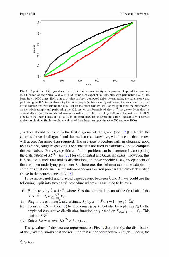
The p-values of this test are represented in Fig. 1. If the distribution of the teststatistic was correctly predicted by the quantiles kn,1−α , then the repartition of the
Page 6 of 41 P. Reynaud-Bouret et al.
Fig. 1 Repartition of the p-values in a K.S. test of exponentiality with plug-in. Graph of the p-valuesas a function of their rank. A n = 40 i.i.d. sample of exponential variables with parameter λ = 20 hasbeen drawn 1000 times. Each time a p-value has been computed either by estimating the parameter λ andperforming the K.S. test with exactly the same sample (in black), or by estimating the parameter λ on halfof the sample and performing the K.S. test on the other half (in red), or by estimating the parameter λ
on the whole sample and performing the K.S. test on a subsample of size n2/3 (in green). Note that theestimated level (i.e., the number of p-values smaller than 0.05 divided by 1000) is in the first case of 0.009,of 0.12 in the second case, and of 0.039 in the third case. Those levels and curves are stable with respectto the sample size: Similar results are obtained for a larger sample size (n = 200 and n = 1000)
p-values should be close to the first diagonal of the graph (see [35]). Clearly, thecurve is above the diagonal and the test is too conservative, which means that the testwill accept H0 more than required. The previous procedure fails in obtaining goodresults since, roughly speaking, the same data are used to estimate λ and to computethe test statistic. For very specific c.d.f., this problem can be overcome by computingthe distribution of KS(1) (see [27] for exponential and Gaussian cases). However, thisis based on a trick that makes distributions, in those specific cases, independent ofthe unknown underlying parameter λ. Therefore, this solution cannot be adapted tocomplex situations such as the inhomogeneous Poisson process framework describedabove in the neuroscience field [8].
To be more careful and to avoid dependencies between λ and Fn, we could use thefollowing “split into two parts” procedure where n is assumed to be even.
(i) Estimate λ by λ = 1/ ¯X, where ¯X is the empirical mean of the first half of the
Xi ’s: ¯X = 2/n∑n/2
i=1 Xi .(ii) Plug in the estimate λ and estimate F0 by u → F (u) = 1 − exp(−λu).
(iii) Form the K.S. statistic (1) by replacing F0 by F , but also by replacing Fn by theempirical cumulative distribution function only based on Xn/2+1, . . . ,Xn. Thisleads to KS(2).
(iv) Reject H0 whenever KS(2) > kn/2,1−α .
The p-values of this test are represented on Fig. 1. Surprisingly, the distributionof the p-values shows that the resulting test is not conservative enough. Indeed, the

Journal of Mathematical Neuroscience (2014) 4:3 Page 7 of 41
test will reject H0 more than required and this procedure is even worse than the firststrategy. Therefore, we turn toward a much more universal strategy, subsampling,thanks to the following result (see the Additional File 1 for the proof).
Proposition 1 Let X1, . . . ,Xp be p i.i.d. variables with c.d.f. F assumed to be con-tinuous. Let Fp be the associated empirical distribution. Assume that F is a consis-tent estimate of F such that
√p sup
x
∣∣F (x) − F(x)∣∣ P−−−→
p→∞ 0. (2)
Then√
p supx
∣∣Fp(x) − F (x)∣∣ L−−−→
p→∞ K.
Therefore, it remains to find F satisfying (2). In most of the parametriccases, and in particular in the exponential case, Assumption (2) does not holdif F is based on the same data as Fp . Assumption (2) may hold if p is muchsmaller than n, the whole sample size, as illustrated by the following strategy.�
�
�
�
Test 1
1. Estimate λ by λ = 1/X, where X is the empirical mean of the Xi ’s on the whole samplesize n.
2. Select randomly a subsample S of the trials with cardinality p = p(n), such thatp(n)/n −→
n→∞ 0 (for instance take p(n) = √n or p(n) = n2/3).
3. Compute on S the following empirical cumulative distribution function:
∀x ≥ 0, FS(x) = 1
p
∑i∈S
1{Xi≤x}.
4. Take k1−α the 1 − α quantile of the asymptotic distribution K.5. Reject H0: “the distribution of the Xi ’s is exponential” whenever
√p sup
x∈R+
∣∣FS(x) − F (x)∣∣ > k1−α,
where for any x ≥ 0,
F (x) = 1 − e−λx .
Technical arguments of Additional File 1 prove that the previous test is of exactlevel α asymptotically. More importantly, in practice this conclusion remains trueeven for relatively small values of n as shown in Fig. 1 illustrated with n = 40. Evenif this test is not as powerful as the one described in [27], it has the main advantageto be almost universal. It can be adapted to most of parametric situations, since theuse of subsampling makes the condition (2) quite easy to fulfill.
We want now to adapt this method to the more general scheme of goodness-of-fittests for counting processes. From now on and whatever the situation, p will always

Page 8 of 41 P. Reynaud-Bouret et al.
correspond to the size of a subsample, i.e., a positive integer much smaller than n thetotal number of observations.
2.2 Aggregated Test of H0: “The Observed Processes Are i.i.d. Poisson Processes”
To fix notation, we consider in the sequel that we observe n i.i.d. trials. Consequently,we have access to N1, . . . ,Nn, n i.i.d. point processes observed on [0, Tmax] repre-senting the n i.i.d. spike trains of a fixed recorded neuron during Tmax seconds.
It is not possible to assess on just one realization whether a point process is a(non necessarily homogeneous) Poisson process or not since the variations of therepartition of the points between different parts of one trial can either be due to non-stationarity or to more complex dependency structures that cannot be studied on justone run.
The first simple way to use the repetition of the trials is to use aggregation, whichcan be viewed as an empirical sum on the point processes. More precisely, the aggre-gated process over the processes N1, . . . ,Np is defined by
Na,p =⋃
i=1,...,p
Ni or equivalently dNa,p =p∑
i=1
dNi.
By classical properties of Poisson processes [4], if the processes are i.i.d. Poissonprocesses with compensator Λ(·), then Na,p is also a Poisson process with compen-sator pΛ(·). This implies that conditionally to the event {Na,p([0, Tmax]) = ntot}, theobserved points of Na,p behave like an ntot i.i.d. sample of c.d.f.
t → F(t) = Λ(t)
Λ(Tmax).
Since F is unknown in our present situation, one has to estimate it, which leads toexactly the same plug-in problem as before. Fortunately, we are able to prove thefollowing result.
Proposition 2 Let N1, . . . ,Np be p i.i.d. Poisson processes with compensator Λ(·),assumed to be continuous, on [0, Tmax]. Let FNa,p([0,Tmax]) be the associated empiricaldistribution, defined for any x by
FNa,p([0,Tmax])(x) = 1
Na,p([0, Tmax])∑
T ∈Na,p
1{T ≤x}, (3)
where Na,p is the aggregated Poisson process. Assume that F (·) is a consistent esti-mate of F(·) = Λ(·)/Λ(Tmax) such that√
Na,p([0, Tmax]
)sup
x∈[0,Tmax]∣∣F (x) − F(x)
∣∣ P−−−→p→∞ 0. (4)
Then √Na,p
([0, Tmax])
supx∈[0,Tmax]
∣∣FNa,p([0,Tmax])(x) − F (x)∣∣ L−−−→
p→∞ K.

Journal of Mathematical Neuroscience (2014) 4:3 Page 9 of 41
Once again, subsampling (i.e., choosing p much smaller than n) gives us estimatesF satisfying (4). Two different approaches lead to two distinct tests. First, let us usethe empirical c.d.f. on the whole sample.�
�
�
�
Test 2
1. Take F as FNa,n([0,Tmax]), the empirical c.d.f. of the whole aggregated process Na,n
over the n trials (see (3)).2. Select randomly a subsample S of the trials with cardinality p = p(n), such that
p(n)/n −→n→∞ 0 (for instance take p(n) = √
n or p(n) = n2/3).
3. Aggregate the p processes in S to form Na,p and FNa,p([0,Tmax]) as in Proposition 2.
4. Take k1−α the 1 − α quantile of the asymptotic distribution K.5. Reject H0: “The n observed processes are i.i.d. (nonnecessarily homogeneous) Poisson
processes” whenever
√Na,p
([0, Tmax]) supx∈[0,Tmax]
∣∣FNa,p([0,Tmax])(x) − F (x)∣∣ > k1−α.
In Additional File 1, we prove that this test is of exact asymptotic level α, as soonas the compensator Λ(·) is continuous and this even if λ(·) does not exist. Howeverits practical performance are poor (see later). A slightly more useful test can be ob-tained by using smoother and more elaborate estimates F satisfying (4). We obtainthe following testing procedure.�
�
�
�
Test 3
1. Select randomly a subsample S of the trials with cardinality p = p(n), such thatp(n)/n tends to 0.
2. Use all the n observed processes to obtain a λ(·) such that, if the processes are Poissonprocesses with intensity λ(·), one can assume that
√p(n)
∫ Tmax
0
∣∣λ(u) − λ(u)∣∣ P−−−−→
p→∞ 0. (5)
3. Take
t → F (t) =∫ t
0 λ(u)du∫ Tmax0 λ(u)du
.
4. Aggregate the p processes in S to form Na,p and FNa,p([0,Tmax]) as in Proposition 2.
5. Take k1−α the 1 − α quantile of the asymptotic distribution K.6. Reject H0: “The n observed processes are i.i.d. (non necessarily homogeneous) Poisson
processes” whenever
√Na,p
([0, Tmax]) supx∈[0,Tmax]
∣∣FNa,p([0,Tmax])(x) − F (x)∣∣ > k1−α.
In Additional File 1, we prove that the previous test is of asymptotic level α.Note that Condition (5) can be demanding and rejection can be due to nonfulfillmentof this condition. For instance, estimates λ based on parametric estimates on a pre-scribed parametric model (such as maximum likelihood estimates for instance, see
Page 10 of 41 P. Reynaud-Bouret et al.
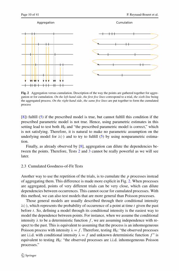
Fig. 2 Aggregation versus cumulation. Description of the way the points are gathered together for aggre-gation or for cumulation. On the left-hand side, the first five lines correspond to a trial, the sixth line beingthe aggregated process. On the right-hand side, the same five lines are put together to form the cumulatedprocess
[8]) fulfill (5) if the prescribed model is true, but cannot fulfill this condition if theprescribed parametric model is not true. Hence, using parametric estimates in thissetting lead to test both H0 and “the prescribed parametric model is correct,” whichis not satisfying. Therefore, it is natural to make no parametric assumption on theunderlying model for λ(·) and to try to fulfill (5) by using nonparametric estima-tion.
Finally, as already observed by [8], aggregation can dilute the dependencies be-tween the points. Therefore, Tests 2 and 3 cannot be really powerful as we will seelater.
2.3 Cumulated Goodness-of-Fit Tests
Another way to use the repetition of the trials, is to cumulate the p processes insteadof aggregating them. This difference is made more explicit in Fig. 2. When processesare aggregated, points of very different trials can be very close, which can dilutedependencies between occurrences. This cannot occur for cumulated processes. Withthis method, we can also test models that are more general than Poisson processes.
Those general models are usually described through their conditional intensityλ(·), which represents the probability of occurrence of a point at time t given the pastbefore t . So, defining a model through its conditional intensity is the easiest way tomodel the dependence between points. For instance, when we assume the conditionalintensity λ to be a deterministic function f , we are assuming independence with re-spect to the past. This is equivalent to assuming that the process is an inhomogeneousPoisson process with intensity λ = f . Therefore, testing H0: “the observed processesare i.i.d. with conditional intensity λ = f and unknown deterministic function f ” isequivalent to testing H0: “the observed processes are i.i.d. inhomogeneous Poissonprocesses.”

Journal of Mathematical Neuroscience (2014) 4:3 Page 11 of 41
More generally, we wish to test a nonparametric hypothesis on the conditionalintensity. An example, more developed in the next section, is the multivariate Hawkesprocess, which models the dependence between the spikes of different neurons viaseveral interaction functions, for which we do not want to give a parametric form. Letus give just a simple expression of this process to illustrate our set-up, with only oneprocess. The classical self-exciting Hawkes process has conditional intensity givenby
λ(t) = λf (t) = μ +∫ t−
−∞h(t − u)dN(u), (6)
where μ is a positive real parameter and h a non negative integrable function withsupport in R
∗+ and with f = (μ,h). For instance, if the function h is supported bythe interval (0,2], then the probability of occurrence at time t randomly depends onthe occurrences of the process on [t − 2, t). Testing whether the process is a classicalself-exciting Hawkes or not can be rephrased as testing whether the process has con-ditional intensity given by the form λf defined in (6), with unknown f . Other famousexamples in biomedical areas such as the multiplicative Aalen intensity or the Coxmodel can be found in [29].
As in the previous subsection, we use the time-rescaling theorem but in a deeperway. Remember that the general time-rescaling theorem [2] states that for any pointprocess N on [0, Tmax] with compensator Λ(·), the point process N = {X = Λ(T ) :T ∈ N} is a Poisson process with intensity 1 on [0,Λ(Tmax)]. Therefore, it is moreinteresting to cumulate the processes after time-rescaling than in the usual time space[0, Tmax]. For general conditional intensity models, Λ(·) is random. Therefore thestate space [0,Λ(Tmax)] is also random in general. Moreover, when we are dealingwith p i.i.d. processes N1, . . . ,Np , each Ni has a different compensator Λi(·) whichdepends on the history of the ith trial. So except in the Poisson case where Λ(·) isdeterministic, we do not apply the same transformation to all the points. We finallyhave to deal with p processes Ni = {X = Λi(T ) : T ∈ Ni} that are Poisson processesof intensity 1, and whose occurrences lie in [0,Λi(Tmax)]. Even if the Λi(Tmax) arei.i.d., they are not equal in general.
This leads to two main remarks. First, it is not possible to aggregate in gen-eral the time-transformed processes since we would aggregate processes with dif-ferent lengths (see Fig. 2). Therefore, Tests 2 and 3 cannot be transferred to themost general case straightforwardly. However, one can cumulate those processesas done in Fig. 2 and this even if the intervals have different lengths. The result-ing process N c,p is therefore a Poisson process with intensity 1 on the random in-terval I = [0,
∑p
i=1 Λi(Tmax)] (see also Additional File 1 for a more precise for-mula and a proof of this statement). The second remark consists in noting that∑p
i=1 Λi(Tmax) being a random quantity, it is not true in general that conditionallyto the total number of points in I , the points of N c,p behave like an i.i.d. uniformsample, and in the sequel we shall need to restrict ourselves to an interval of the form[0,pθ ] with a deterministic bound pθ , which is with high probability, smaller than∑p
i=1 Λi(Tmax).

Page 12 of 41 P. Reynaud-Bouret et al.
Besides we have to deal with estimation of unknown transformations Λi(·). Forthis purpose, we introduce estimates of the type t → Λi(t) = ∫ t
0 λi (u)du, where λi (·)estimates λi(·), the conditional intensity of the ith process Ni . We obtain a cumulateprocess N c,p built from the Λi(·)’s. We have the following equivalent to Proposi-tion 2.
Theorem 1 Let N1, . . . ,Np be p i.i.d. processes with respective conditional intensityλi(·). Assume that there exist nonnegative estimates λi (·) of λi(·) such that
p−1/2
(p∑
i=1
∫ Tmax
0
∣∣λi (u) − λi(u)∣∣du
)P−−−→
p→∞ 0. (7)
Then, for all θ > 0 such that E(Λ1(Tmax)) > θ ,
√N c,p
([0,pθ ]) supu∈[0,1]
∣∣∣∣ 1
N c,p([0,pθ ])∑
X∈N c,p,X≤pθ
1{X/(pθ)≤u} − u
∣∣∣∣ L−−−→p→∞ K.
It is now easy to turn this result into an operational test, using subsampling.�
�
�
�
Test 4
1. Select randomly a subsample S of the trials with cardinality p = p(n), such that p(n)/n
tends to 0.2. Use all the n observed processes to obtain a f such that if λ = λf , one can assume that
p(n)−1/2
(p(n)∑i=1
∫ Tmax
0
∣∣(λf)i (u) − (λf )i (u)
∣∣du
)P−−−→
n→∞ 0. (8)
3. For all i in S, take
Λi (t) =∫ t
0
((λ
f)i (u)
)+du,
and change time of the ith process accordingly to obtain Ni = {X = Λi (T ) : T ∈ Ni} on[0, Λi (Tmax)].
4. Cumulate the p processes Ni for i in S to form N c,p .5. Take k1−α the 1 − α quantile of the asymptotic distribution K.6. Fix θ > 0, strictly smaller than p−1 ∑
i∈S Λi (Tmax).7. Reject H0: “The n observed processes are i.i.d. processes with conditional intensity of the
form λf and unknown f ” whenever
√N c,p
([0,pθ]) supu∈[0,1]
∣∣∣∣ 1
N c,p([0,pθ])∑
X∈N c,p,X≤pθ
1{X/(pθ)≤u} − u
∣∣∣∣ > k1−α.
In Additional File 1, we prove that the previous test is of exact asymptotic levelα as soon as E(Λi(Tmax)) > θ . There exists a simpler form of this test when dealing

Journal of Mathematical Neuroscience (2014) 4:3 Page 13 of 41
with Poisson processes since in this case compensators do not depend on i.�
�
�
�
Test 5
1. Select randomly a subsample S of the trials with cardinality p = p(n), such that p(n)/n
tends to 0.2. Use all the n observed processes to obtain a λ(·), such that if the processes are Poisson
processes with intensity λ(·), one can assume that
√p(n)
(∫ Tmax
0
∣∣λ(u) − λ(u)∣∣du
)P−−−→
n→∞ 0. (9)
3. Take
Λ(t) =∫ t
0
(λ(u)
)+du,
and change time of the ith process accordingly to obtain Ni = {X = Λ(T ) : T ∈ Ni} on[0, Λ(Tmax)].
4. Cumulate the p processes in S to form N c,p .5. Take k1−α the 1 − α quantile of the asymptotic distribution K.6. Fix θ > 0, strictly smaller than Λ(Tmax).7. Reject H0: “The n observed processes are i.i.d. non necessarily stationary Poisson pro-
cesses” whenever√N c,p
([0,pθ]) supu∈[0,1]
∣∣∣∣ 1
N c,p([0,pθ])∑
X∈N c,p,X≤pθ
1{X/(pθ)≤u} − u
∣∣∣∣ > k1−α.
This test, as a special case of Test 4, is also of exact asymptotic level α as soon asΛ(Tmax) > θ . Tests 4 and 5 are more powerful to detect dependencies or to reject thePoisson assumption than Tests 2 or 3, as we will see later.
As for Test 3, and for exactly the same reasons, we want to find nonparametricestimates satisfying (8) or (9). We provide in the next section powerful tools to dealwith this problem and theoretical guarantees of performance of these estimates.
3 Nonparametric and Adaptive Estimation
3.1 Why Is Adaptive Estimation Useful?
Nonparametric estimation, and in particular nonparametric estimation of Poisson pro-cess intensity, is at the root of most of the data analyses performed on spike trains.Indeed, peristimulus time histograms (PSTH) [36] are usually the first graphical rep-resentations of an experiment. Those histograms have usually a fixed length for eachinterval (typically 10 ms) and are quite noisy from a statistical point of view (see,for instance, the representations of [8]). Therefore, there have been several attemptsto provide smoother estimates, either by kernel estimates (see, for instance, [30]) orby projection on an orthonormal basis (see, for instance, [7] for the use of splines).These methods provide a first illustration of the data with as few assumptions as pos-sible on the underlying “true” firing rate. They are originally not linked at all to anystatistical or probabilistic models and constitute descriptive statistics. In particular,
Page 14 of 41 P. Reynaud-Bouret et al.
no parametric assumption on the underlying intensity is made at this step, the para-metric model and its associated maximum likelihood estimator (MLE) being givenin a second time once the shape of the curve is guessed [8]. Because of this lack ofparametric assumption, those estimates seem to be the best candidates at first glancefor the estimate λ that needs to be plugged in Tests 3 or 5.
However, the problem of the convergence rate remains. In all these methods, thereis a tuning parameter that needs to be chosen: it is the length of the interval for his-tograms, the bandwidth in kernel rules or the number of coefficients in the orthonor-mal expansion. The problem of the choice of this parameter has first been tackledvery roughly in the neuroscience literature by choosing a fixed value. On the realdata presented here or on the ones in [8], it was usually considered that a bandwidthof 50 or 100 ms was a good choice. However, such a very rough choice cannot guar-antee a convergence rate when n goes to ∞. Indeed let us look more closely at thekernel estimate.
For the i.i.d. observed point processes N1, . . . ,Nn, the kernel estimate with kernelK and bandwidth h is given by
λKhn (x) = 1
n
n∑i=1
∫Kh(x − u)dNi(u) = 1
n
∫Kh(x − u)dNa,n(u), (10)
where Na,n is the corresponding aggregated process and where Kh(u) = (1/h) ×K(u/h). If we assume that the observed processes are inhomogeneous Poisson pro-cesses with intensity λ, Na,n is also an inhomogeneous Poisson process with intensitynλ and, therefore,
E[λKh
n (x)] = (Kh � λ)(x), ∀x ∈ R,
where � denotes the convolution product. So, the expectation of λKhn constitutes a
regularized approximation of λ(·). To measure the performance of λKhn , we compute
its L2-risk (see further details in Additional File 2):
E∥∥λKh
n − λ∥∥2
2 = ‖Kh � λ − λ‖22 + ‖λ‖1
nh‖K‖2
2, (11)
which is classically interpreted as a bias-variance decomposition. Therefore, if h isfixed, the variance term goes to 0 whereas the bias remains fixed so that the L2-riskof the estimate does not go to 0. Consequently, a fixed choice for the bandwidthis not convenient and it is essential to choose h = h(n) tending to 0 with n. Thedependence of h with respect to n is a problem that has been extensively studied inthe density framework, a setting close to the present one since conditionally to thetotal number of points, the observed points of Na,n behave like an i.i.d. sample ofdensity λ(·)/Λ(Tmax). We refer the reader to [37] for a review. The main conclusionof such a study is that if λ is regular and if the regularity is known then we are able tochoose h(n) such that the L2-risk tends to 0 at a known rate of convergence dependingon the regularity. Furthermore, the larger the regularity, the faster the rate. Typically,if the r th derivative of λ is bounded in the L2 sense, then it is possible to choose K
Journal of Mathematical Neuroscience (2014) 4:3 Page 15 of 41
and1 h(n) � n−1/(2r+1) such that the L2-risk behaves as
E∥∥λKh
n − λ∥∥2
2 � n−2r/(2r+1).
In this setting, this choice can be applied to Tests 3 and 5, since the Markov inequalityimplies that (5) or (9) are satisfied with p(n) = nδ and δ < (2r)/(2r + 1). The choicer = 1 gives δ < 2/3 and r = 2 gives δ < 4/5.
Of course, in practice the choice of the bandwidth is capital. Since the smooth-ness of λ is unknown, the practitioner cannot use the previous choice. Furthermore,guessing the order of magnitude of h(n) is not enough to achieve good performancesince the leading constant plays an essential role. Hence, the theoretical considera-tions developed before do not solve the practical problem. Several directions havebeen proposed to overcome this problem. One of the most famous ones consists inusing leave-one-out or other cross-validation methods [30, 38]: among a finite fam-ily of fixed bandwidths, such methods choose the best one in an asymptotic setting.However, to our knowledge, nothing can be said when the family of bandwidths isnot fixed and some bandwidths tend to 0 with n. It is not clear at all that the resultingestimate achieves a prescribed rate and, therefore, it cannot be used for the proposedtests in particular. Other methods based on the rule of the thumb (and variations of it)have been proposed in the density or the Poisson setting [8, 39], and in this case theresulting bandwidth is of the form h(n) = Cn−1/5 for various possible choices of theconstant C. Generally, those choices lead to poor results as noted by [8] (see also ourthe simulation study).
Adaptive estimation [37] aims at tuning in a data-driven way the unknown pa-rameters of those methods (kernels, histograms, etc.) such that the resulting estimatehas good practical performance and a guaranteed convergence rate. The adaptive es-timates are usually mathematically proved to achieve the best possible rate of conver-gence and this even if the regularity is unknown. Moreover, they do not depend on anyrestrictive assumption such as, for instance, some parametric assumption. The onlyassumption lies in the underlying probabilistic model (for instance, one assumes thatthe processes are inhomogeneous Poisson processes). Their reconstructions are there-fore much more trustworthy than other methods for which those extra assumptionsmay not be fulfilled. As a conclusion, adaptive estimates constitute ideal candidatesto be plugged in Tests 3, 4, or 5.
The main aim of next subsections is therefore to present adaptive estimates in thePoisson or in the Hawkes model that will have these good properties.
3.2 Adaptive Estimation for Poisson Processes
3.2.1 Kernel Estimates
As mentioned previously, the Poisson setting is very close to the density setting. Inthe density setting, the main adaptive method for choosing a bandwidth is the Lepski
1If (an)n≥0 and (bn)n≥0 are two sequences, a(n) � b(n) means that there exists two positive constantsc1, c2 such that for all n ≥ 0, c1an ≤ bn ≤ c2an .

Page 16 of 41 P. Reynaud-Bouret et al.
method, which has been recently updated to the multidimensional framework andto deal with the problem of choosing the leading constant of the bandwidth. Due toGoldenshluger and Lepski [40], it is referred in the sequel as the GL method. Wepropose here to adapt this method to the Poisson setting in the following way and toprove its adaptive properties.
We consider a set of bandwidths H and their corresponding kernel estimates λKhn .
The bias-variance decomposition shows that the parameter h which minimizes theright-hand side of (11) with respect to h ∈H is the best possible choice. It is called theoracle bandwidth: since it depends on λ(·), it cannot be used in practice. To proposea data-driven choice of the bandwidth by a GL method, we define for any h,h′ ∈H:
λh,h′n (x) := 1
n
∑T ∈Na,n
(Kh � Kh′)(x − T ) = (Kh � λ
Kh′n
)(x), ∀x ∈R,
then for η > 0, we set
A(h) := suph′∈H
{∥∥λh,h′n − λ
Kh′n
∥∥2 − (1 + η)(1 + ‖K‖1)‖K‖2
√Na,n([0, Tmax])
n√
h′
}+.
The Additional File 2 shows that A(h) constitutes a good estimate of the bias term(see (11)). Finally, we select the data-driven bandwidth as follows:
h := arg minh∈H
{A(h) + (1 + η)(1 + ‖K‖1)‖K‖2
√Na,n([0, Tmax])
n√
h
}, (12)
which allows us to estimate λ(·) by using
λGLn := λ
Kh
n . (13)
Note that in (12), ‖K‖22N
a,n([0, Tmax])/(n2h) is an unbiased estimate of the varianceterm in (11) and therefore the previous criterion mimics the bias-variance decompo-sition of the risk of λ
Khn up to some multiplicative constant. Once K , H and η are
chosen, we obtain a turnkey procedure. The following theoretical result justifies ourprocedure.
Theorem 2 If H ⊂ {D−1 : D = 1, . . . ,Dmax} with Dmax = δn for some δ > 0, and if‖λ‖∞ < ∞, then,
E∥∥λGL
n − λ∥∥2
2 ≤ C1 infh∈H
{‖Kh � λ − λ‖2
2 + ‖λ‖1
nh‖K‖2
2
}+ C2n
−1,
where C1 is a constant depending on ‖K‖1 and η and C2 is a constant depending onδ, η, ‖K‖2, ‖K‖1, ‖λ‖1, and ‖λ‖∞.
Theorem 2 combined with (11) shows that our procedure mimics the performanceof the oracle up to the constant C1 and up to the term C2n
−1, which is negligible whenn goes to +∞. It is classically called an oracle inequality, which is the main property
Journal of Mathematical Neuroscience (2014) 4:3 Page 17 of 41
of adaptive estimates. In particular, one can take the family H = {1, . . . , �δn�−1},which grows with n and it is possible to select a bandwidth tending to 0 with n. If ther th derivative of λ(·) is bounded in L2, then the choice h(n) � n−1/(2r+1) is in thefamily H and the oracle inequality gives straightforwardly that
E∥∥λGL
n − λ∥∥2
2 � n−2r/(2r+1),
which is the optimal rate of convergence over such spaces. This rate is achieved, evenif we do not know in advance the regularity r of λ, which is from a theoretical pointof view the main improvement with respect to the theory described in the previoussubsection.
If K is the Gaussian kernel, then ‖K‖1 = 1 and ‖K‖2 = 2−1/2π−1/4. Moreover,Kh �Kh′ = K√
h2+h′2 and a straightforward computation shows that explicit formula
for ‖λh,h′n − λ
Kh′n ‖2 are also available. It is consequently very easy to implement the
method, the computational cost being almost of the same order as cross-validation.We will see in the simulation study that this practical choice is also quite robust.
3.2.2 Histograms
In the Poisson set-up, there are several ways to select data-driven partitions that leadto adaptive histogram estimates. For instance, one can use model selection as in [41].Model selection can either select a regular partition or an irregular partition on agrid. When regular partitions are considered, the resulting estimator satisfies an ora-cle inequality similar to the oracle inequality established in Theorem 2 for the kernelrule combined with the GL method. Indeed the bin for the histograms plays exactlythe same role as the kernel bandwidth. Therefore, it leads to similar theoretical per-formance, except that the histograms cannot become smooth enough to guarantee anoptimal convergence rate for regular intensities (namely r > 1). Therefore, the choiceof regular partitions is probably not the best one and one may prefer the GL method.The data-driven choice of the partition becomes much more interesting when the par-tition is not forced to be regular. Indeed irregular partitions can capture a fast increaseof the firing rate followed very quickly by a fast decrease at some particular momentof the experiment, without leading to too noisy estimates as the classical PSTH, sinceover smoother periods, the length of the interval can be much larger. However, themethod of [41] is too time consuming to be really considered in practice. Anotherpossible direction is the context of Markov modulated Poisson processes [42], wherethe algorithms are also quite time consuming without ensuring any adaptive prop-erty in terms of convergence rate (despite some possible interpretation with respectto hidden Markov processes).
However, and as already noticed in [41], it is possible in certain cases to interpreta model selection estimate as a thresholding rule. We hereafter illustrate in a simplercase, the method developed in [43]: If λ(·) ∈ L2, we can decompose it on the Haarbasis,
λ =+∞∑
j=−1
∑k∈Z
βj,kψj,k,

Page 18 of 41 P. Reynaud-Bouret et al.
where ψ−1,k(·) = φ(· − k) with φ = 1[0,1) the Haar father wavelet and whereψj,k(·) = 2j/2ψ(2j (· − k)) for j ≥ 0 with ψ = 1[0,1/2) − 1[1/2,1) the Haar motherwavelet. The βj,k’s are the unknown coefficients of λ(·) and are given by
∀j ≥ −1, k ∈ Z, βj,k =∫
ψj,k(x)λ(x)dx.
These coefficients can therefore be unbiasedly and consistently estimated by
∀j ≥ −1, k ∈ Z, βj,k = 1
n
∫ψj,k(x)dNa,n(x).
Given a fixed finite subset of indices m, we obtain an easily computable estimate ofλ(·):
λmn =
∑(j,k)∈m
βj,kψj,k.
Since the Haar basis is piecewise constant, the previous estimate is also piecewiseconstant on a certain partition P depending on m. A data-driven choice of m there-fore leads to a data-driven choice of the partition that can be irregular. Let us fix anarbitrary highest level of resolution j0 such that 2j0 ≤ n < 2j0+1 and let us considerthe L2-risk of λm
n such that if (j, k) ∈ m then j ≤ j0. The bias-variance decomposi-tion of λm
n can be written as follows:
E[∥∥λm
n − λ∥∥2] =
∑(j,k)/∈m
β2j,k +
∑(j,k)∈m
Var(βj,k)
=∑j>j0
∑k
β2j,k +
∑j≤j0
∑k
[β2
j,k1(j,k)/∈m + vj,k1(j,k)∈m
], (14)
where
vj,k := Var(βj,k) = 1
n
∫ψ2
j,k(x)λ(x)dx.
Hence, the best subset m is the set of indices (j, k) such that βj,k >√
vj,k . This is theoracle choice. A possible data-driven way to choose the indices (j, k) is to choose theindices such that βj,k are larger than a certain threshold ηjk depending on an estimateof the variance vj,k . The choice advertised in practice in [43] is
ηj,k =√
2γ ln(n)vj,k + γ ln(n)2j/2
3nwhere vj,k = 1
n2
∫ψ2
j,k(x)dNa,n(x). (15)
Then we obtain the following thresholding estimator:
λThn =
j0∑j=−1
∑k
βj,k1{|βj,k |>ηj,k}ψj,k. (16)
In [43], it has been proved that a slight modification of this estimate satisfies an or-acle inequality in the same spirit as Theorem 2. It also generalizes this estimate by
Journal of Mathematical Neuroscience (2014) 4:3 Page 19 of 41
considering general biorthogonal bases instead of the Haar basis, leading to smoothestimates (see [43, 44]). In this case, for a slight modification of the threshold, the re-sulting estimate has the same convergence rates as the kernel estimate combined withthe GL method, up to some logarithmic term, as soon γ > 1. The choice γ < 1 hasbeen shown to lead to bad convergence rates and the choice γ = 1 has been shownto work well on extensive simulations in both [43, 44]. This method is easily imple-mentable leading to very fast algorithms that are in particular faster than algorithmsbased on the GL method.
3.2.3 More Sophisticated Procedures
Thresholding rules and irregular partitions overcome a drawback of kernel estimatesthat suffer from a lack of spatial adaptivity on the time axis. Several attempts havebeen proposed to build more local choices of the bandwidth (see [30] for instance),but to our knowledge no mathematical proof of this spatial adaptation has been estab-lished, whereas histograms and in particular the previous Haar thresholding estimatorcan adapt the length of the bin to the heterogeneity of the data. But the resulting esti-mator is not smooth at all. As explained, we can consider a smoother wavelet basis,but this extension does not completely address the issue.
The best alternative, to our knowledge, when the support of λ(·) is known andbounded (here [0, Tmax]) and when λ(·) does not vanish for a significant period oftime, is due to Willett and Nowak [45]. Their method is quite intricate to describe. In-formally, a penalized log-likelihood criterion is used to select a piecewise polynomial.Both the partition and the degree of each polynomial on each interval of the partitionare free (on a very refined grid of resolution). Willett and Nowak have proved thatsuch an estimator achieves optimal rates of convergence for various classes of regu-larity and in an adaptive way. From a practical point of view, a dyadic tree algorithmis used. Its complexity is much smaller than a full model selection method on thesame piecewise polynomial family of models. It is a bit more complex than a thresh-olding algorithm, but there exist a program (FreeDegree) in Matlab interfacedwith C which makes its use in practice quite easy. For a more complete description ofthe method, we refer to [45]. Note that in practice because of its adaptive properties,this estimator is able to be piecewise constant when the true intensity is piecewiseconstant but also very smooth (with high degree for the polynomials) when the un-derlying intensity is smooth and when the number of points is sufficient. It is alsoable to be spatially adaptive, the underlying data-driven partition being irregular. Inthe sequel, we denote this method λWN
n .
3.3 Adaptive Estimation for Hawkes Processes
If inhomogeneous Poisson processes can model nonstationary data, they are notappropriate to model dependencies between points. However, several studies haveestablished potential dependence of spike occurrences for different neurons. Thishas been detected via descriptive statistics, via independence tests for a given fixedmodel or via model-free independence tests based on permutations (also called trials-shuffling) [5, 6, 13, 15, 22, 46].
Page 20 of 41 P. Reynaud-Bouret et al.
One simple model of dependency is the multivariate Hawkes process, which is thepoint process equivalent to the auto-regressive model. It has first been introduced byHawkes [47], as a self-exciting point process, that is useful in particular in seismology(see, for instance, [23]). It has also been used to model positions of motifs along theDNA molecule [48, 49]. In neuroscience, it explicitly appears in the 1980s with [19]and is close in spirit to [50, 51], with the additional advantage of modeling potentialfeed-back between the neurons.
The multivariate Hawkes process (see, for instance, [52] or [4]) models the instan-taneous firing rates of M different neurons, with spike trains N(1), . . . ,N(M), wherethe conditional intensity of the mth point process is defined for any t ≥ 0 by
λ(m)(t) =(
ν(m) +M∑
�=1
∫ t−
−∞h
(m)� (t − u)dN(�)(u)
)+
=(
ν(m) +M∑
�=1
∑T�∈N(�),T�<t
h(m)� (t − T�)
)+. (17)
In (17), the ν(m)’s are positive parameters representing the spontaneous firing ratesand the h
(m)� ’s are the interaction functions and have support included into R
∗+. Moreprecisely, before the first occurrence of the multivariate process, the N(m)’s behavelike homogeneous Poisson processes with constant intensities ν(m). The first occur-rence (and the next ones) affects all the processes by increasing or decreasing theconditional intensity via the interaction functions h
(m)� ’s. For instance, if h
(m)� takes
large positive values in the neighborhood of the delay d and is null elsewhere, thenafter the delay d of one occurrence of N(�), the probability to have a new occurrenceof N(m) will significantly increase: The process N(�) excites the process N(m). On thecontrary, if h
(m)� is negative around d , then after the delay d of one occurrence of N(�),
the probability to have a new occurrence of N(m) will significantly decrease: The pro-cess N(�) inhibits the process N(m). Note in particular that the functions h
(m)m ’s model
self-interactions.The Hawkes process as described above cannot really model nonstationary data.
Indeed, when t grows (and under conditions on the interaction functions), the processconverges quite quickly toward an equilibrium, which is stationary (see, for instance,[52, 53], and the references therein). If these conditions are not satisfied, the numberof points in the process grows too fast to be a realistic model for spike trains anyway.Hence, Hawkes processes as defined in (17) cannot model nonstationary data, but canmodel dependent data.
Therefore, we fix an interval [T1, T2] ⊂ [0, Tmax], typically an interval where allthe estimated mean firing rates seem constant. The aim is to estimate on this interval
f ∗ = ((ν(m)
)m=1,...,M
,(h
(m)�
)�,m=1,...,M
),
where it is assumed that the interaction functions are bounded with support in [0,A]with T1 > A.
Journal of Mathematical Neuroscience (2014) 4:3 Page 21 of 41
Inference for Hawkes models based on the likelihood can be found in the literature,in particular, for parametric models [23, 49]. However, in neuroscience, for flexibility,the used parametric models are based on a large number of parameters. Therefore,they require several thousand spikes per neuron to be observed in a stationary wayto achieve good estimation [19]. Classical model selection based on AIC and BICcriteria has also been used to select the number of knots for the spline estimate [21,48, 54]. However, these criteria do not adapt well to irregular functions. This is thereason why alternative nonparametric adaptive inference has recently been developedin such models. The univariate case (M = 1) has been studied in [55], where rates ofconvergence depending on the underlying regularity of the self-interaction functionhave been derived. We can also mention the alternatives proposed in [20, 56] but notheoretical validation is provided in those works.
A multivariate approach, valid for very general counting processes includingHawkes processes and based on �1 penalties, has been recently developed in [57].Based on minimization of convex criteria, its computational cost is more reasonablethan procedures proposed in [55] and it is also proved to satisfy oracle inequalities.We shall detail this method in the case of Hawkes processes and with piecewise con-stant estimates of the underlying interaction functions.
In the next section that can be skipped at first reading, we describe the methodin a technical way. Then we give heuristic arguments to understand more deeply thepresented method (see also [58] for a quicker view on this estimate). In particular, themethod does not rely on the likelihood, but on a least-square contrast, which can bereinterpreted in terms of JPSTH [59].
3.3.1 Intensity Candidates and Least-Square Contrast on One Trial
We first propose a conditional intensity candidate. So for any f ∈H with
H = (R×L2
([0,A])M)M
={f = ((
μ(m),(g
(m)�
)�=1,...,M
)m=1,...,M
) : g(m)� with support in (0,A]
and ‖f ‖2 =∑m
(μ(m)
)2 +∑m
∑�
∫ A
0g
(m)� (t)2dt < ∞
},
we consider the predictable transformation ψ(f ) = (ψ(1)(f ), . . . ,ψ(M)(f )) suchthat
∀t > 0, ψ(m)t (f ) = μ(m) +
M∑�=1
∫ t−
−∞g
(m)� (t − u)dN�(u). (18)
Note that λ(m) = [ψ(m)(f ∗)]+. Therefore, for each m, ψ(m)(f ) can be considered asa good intensity candidate as long as it is close enough to the conditional intensityλ(m) (even if ψ(m)(f ) takes negative values). We measure the distance between ψ(f )

Page 22 of 41 P. Reynaud-Bouret et al.
and λ by using the classical L2-norm ‖ · ‖:
∥∥ψ(f ) − λ∥∥2 =
M∑m=1
∫ T2
T1
[ψ
(m)t (f ) − λ(m)(t)
]2dt
=M∑
m=1
∫ T2
T1
[ψ
(m)t (f ) − [
ψ(m)t
(f ∗)]
+]2
dt. (19)
Depending on f ∗, the right-hand side is not observable. But minimizing the last ex-pression with respect to f is equivalent to minimizing f �−→ γ (f ) with
γ (f ) = −2M∑
m=1
∫ T2
T1
ψ(m)t (f )λ(m)(t)dt +
M∑m=1
∫ T2
T1
[ψ
(m)t (f )
]2dt.
But by definition of the conditional intensity, γ (f ) is close to γ (f ) with
γ (f ) = −2M∑
m=1
∫ T2
T1
ψ(m)t (f )dN(m)(t) +
M∑m=1
∫ T2
T1
[ψ
(m)t (f )
]2dt, (20)
which is called the least-square contrast. This expression is observable and can beminimized if f is parameterized by a fixed number of parameters.
One particular parameterization, that is used in practice, is obtained when eachfunction g
(m)� is a piecewise constant function written as
g(m)� =
K∑k=1
am,�,kδ−1/21((k−1)δ,kδ], (21)
where δ > 0 is the size of the bin and K the number of bins. So we have Kδ = A. Theam,�,k’s are the renormalized coefficients of g
(m)� on the regular partition of size K .
Since f → ψ(m)(f ) is linear, one obtains
∀t > 0, ψ(m)t (f ) = μ(m) +
M∑�=1
K∑k=1
am,�,kδ−1/2N(�)
([t − kδ, t − (k − 1)δ
)),
still for f = ((μ(m), (g(m)� )�=1,...,M)m=1,...,M). Let us denote by a(m) the column vec-
tor such that (a(m)
)′ = (μ(m), am,1,1, . . . , am,1,K, am,2,1, . . . , am,M,K
), (22)
where ′ denotes the transpose. Then one can write
∀t > 0, ψ(m)t (f ) = (Rct )
′a(m), (23)
with Rct being the renormalized instantaneous counts given by
(Rct )′ = (
1, δ−1/2(c(1)t
)′, . . . , δ−1/2(c(M)
t
)′),

Journal of Mathematical Neuroscience (2014) 4:3 Page 23 of 41
and with c(�)t being the vector of instantaneous counts with delay of N(�), i.e.,
(c(�)t
)′ = (N(�)
([t − δ, t)), . . . ,N(�)
([t − Kδ, t − (K − 1)δ
))).
Hence, by (23), proposing ψ(m)t (f ) as a candidate for the intensity λ(m) of N(m)
amounts to proposing a linear combination of instantaneous counts with delay tomodel the probability of the next occurrence of a point in N(m).
Now, minimizing γ (f ) over such piecewise constant functions is equivalent, bylinearity, to minimizing
γ (f ) =M∑
m=1
(−2(a(m)
)′b(m) + (a(m)
)′Ga(m))
with respect to the vectors a(m). The vector b(m) is observable and is given by
(b(m)
)′ =(∫ T2
T1
Rct dN(m)(t)
)′
= (N(m)
([T1, T2]), δ−1/2n′
m,1, . . . , δ−1/2n′
m,M
),
where
nm,� =(∫ T2
T1
N(�)([
t − kδ, t − (k − 1)δ))
dN(m)(t)
)k=1,...,K
and
G =∫ T2
T1
Rct (Rct )′dt.
Note that the kth component of nm,� is the number of couples (x, y) with x ∈N(m) ∩[T1, T2], y ∈ N(�) and (y −x) ∈ ((k −1)δ, kδ] and G is a symmetric matrix ofsize 1 + MK whose components are the integrated covariations of the renormalizedinstantaneous counts. The solution of this minimization problem is easily available:If G is invertible,
∀m = 1, . . . ,M, a(m) = G−1b(m). (24)
Heuristic arguments show that (24) is a natural expression. We can indeed informallywrite for any m that
dN(m)(t) � λ(m)(t)dt + noise � ψ(m)t
(f ∗)dt + noise,
assuming that at time t , the intensity is strictly positive. By linearity of ψ(m), one canalso write that
dN(m)(t) � (Rct )′a(m)∗ + noise,
Page 24 of 41 P. Reynaud-Bouret et al.
where a(m)∗ are the coefficients corresponding to f ∗, assuming that f ∗ can be codedin this way. Finally, we obtain
∫ T2
T1
Rct dN(m)(t) = b(m) �∫ T2
T1
Rct (Rct )′a(m)∗ dt + noise � Ga(m)∗ + noise,
showing that the estimate given in (24) should be a convenient preliminary estimate.
3.3.2 Least-Square Estimates on Several Trials and Connections with JPSTH andCross-Correlograms
We observe now n trials and, therefore, we have access to (N(1)i , . . . ,N
(M)i )i=1,...,n an
i.i.d. sample of a multivariate point process on [T1, T2]. Each trial has its own history.So to each trial i, we can associate as in the previous subsection the matrix G, thevectors b(m) and so on. Depending on the trial i, we denote them G(i), b(m,i) and soon. The least-square contrast for these n × M spike trains can then be written as
γn(f ) =M∑
m=1
(−2
(a(m)
)′(
n∑i=1
b(m,i)
)+ (
a(m))′(
n∑i=1
G(i)
)a(m)
)(25)
whose solution is given by
∀m = 1, . . . ,M, a(m) =(
n∑i=1
G(i)
)−1( n∑i=1
b(m,i)
). (26)
The quantity (∑n
i=1 b(m,i)) can be reinterpreted in terms of cross-correlograms andjoint-PSTH, following [59]. Indeed we can write(
n∑i=1
b(m,i)
)′= ([
N(m)]a,n([T1, T2]
), δ−1/2n′
m,1, . . . , δ−1/2n′
m,M
),
where for any �,
nm,� =n∑
i=1
(∫ T2
T1
N(�)i
([t − kδ, t − (k − 1)δ
])dN
(m)i (t)
)k=1,...,K
,
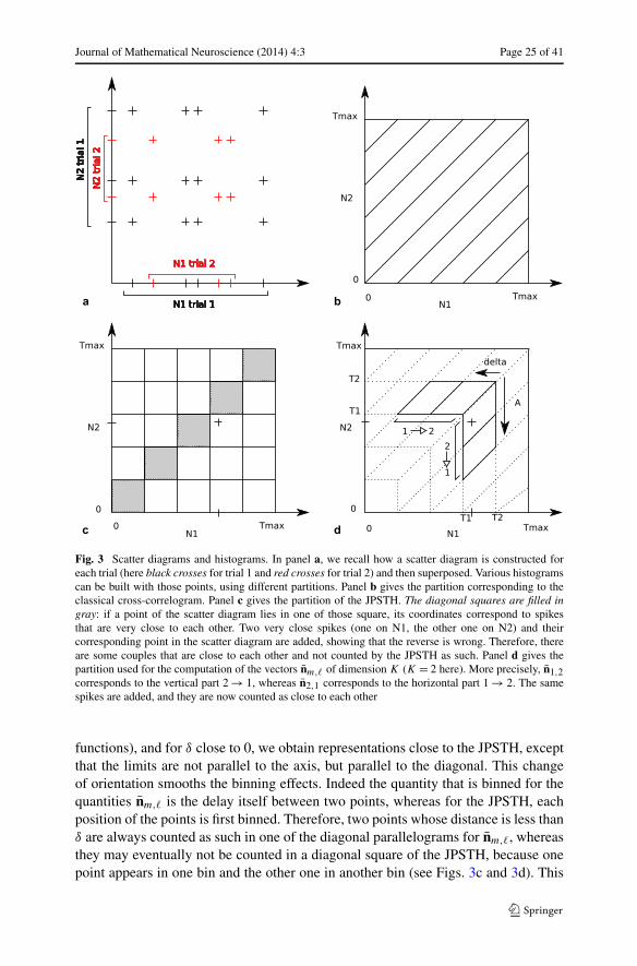
and [N(m)]a,n is the aggregated process over all the n trials for the mth neuron. Thequantity nm,� can be reinterpreted as a particular histogram based on the joint peri-stimulus time scatter diagram as the JPSTH or the cross-correlogram (see Fig. 1 of[59] and Fig. 3 of the present article). More precisely as detailed in Fig. 3, the countsnm,� are close to a cross correlogram except that representations are not based onsquares but on herringbones. Local features are then preserved, as for the JPSTH.Furthermore, the elements of the partition have the same area and can therefore becompared more easily. Besides, for small disjoint intervals [T1, T2] with an increas-ing parameter A (corresponding to the maximal size of the support of the interaction
Journal of Mathematical Neuroscience (2014) 4:3 Page 25 of 41
Fig. 3 Scatter diagrams and histograms. In panel a, we recall how a scatter diagram is constructed foreach trial (here black crosses for trial 1 and red crosses for trial 2) and then superposed. Various histogramscan be built with those points, using different partitions. Panel b gives the partition corresponding to theclassical cross-correlogram. Panel c gives the partition of the JPSTH. The diagonal squares are filled ingray: if a point of the scatter diagram lies in one of those square, its coordinates correspond to spikesthat are very close to each other. Two very close spikes (one on N1, the other one on N2) and theircorresponding point in the scatter diagram are added, showing that the reverse is wrong. Therefore, thereare some couples that are close to each other and not counted by the JPSTH as such. Panel d gives thepartition used for the computation of the vectors nm,� of dimension K (K = 2 here). More precisely, n1,2corresponds to the vertical part 2 → 1, whereas n2,1 corresponds to the horizontal part 1 → 2. The samespikes are added, and they are now counted as close to each other
functions), and for δ close to 0, we obtain representations close to the JPSTH, exceptthat the limits are not parallel to the axis, but parallel to the diagonal. This changeof orientation smooths the binning effects. Indeed the quantity that is binned for thequantities nm,� is the delay itself between two points, whereas for the JPSTH, eachposition of the points is first binned. Therefore, two points whose distance is less thanδ are always counted as such in one of the diagonal parallelograms for nm,�, whereasthey may eventually not be counted in a diagonal square of the JPSTH, because onepoint appears in one bin and the other one in another bin (see Figs. 3c and 3d). This
Page 26 of 41 P. Reynaud-Bouret et al.
problem of information loss when binning is involved has already been discussed forthe coincidence counts [15].
JPSTH and cross correlograms have been used for a long time in neuroscience,without links with any model. The formula (26), for the least-square estimate, showsthe link between those descriptive statistics (more precisely the nm,�’s) and the pa-rameters of the Hawkes model. To recover the parameters, we need, in particular, toinverse the matrix (
∑ni=1 G(i)). This matrix quantifies for instance the following situ-
ation. Assume that M = 3 and that the interaction functions h(1)2 and h
(2)3 are large on
[0, δ] and null elsewhere. We also assume that all the other interaction functions arenull. In this situation, n1,3 (or at least its first coordinate) will be large even if thereis no direct interaction from N3 on N1. The matrix (
∑ni=1 G(i)) cumulates all these
features (and also the fixed effect due to the spontaneous parameter, which needs tobe subtracted) and inverting it enables us to find an estimate of the true interactions.See also [58] for a more visual transcription.
Note, however, that even if many coefficients are null as in the above describedsituation, due to the random noise, the estimates a(m) have non-zero coordinates al-most surely. Therefore, it is difficult to interpret the resulting estimate in terms offunctional connectivity graph [58]. Moreover, if we wish to capture all the features,it is preferable to take A large and δ small. Therefore, the number of parameters ofthe model, depending on K = Aδ−1, increases. With a small number of trials n anda small interval [T1, T2], the least-square estimate is doomed to be quite poor as theMLE [19].
To remedy these problems, we now consider �1 penalization to find a nonparamet-ric estimate with adaptive properties and prescribed convergence rate.
3.3.3 Lasso Estimate
The Lasso method as developed by [57], is based on the following penalized least-square criterion, reformulated here in the context of n i.i.d. trials: for any m =1, . . . ,M ,
a(m) ∈ arg mina(m)
(−2
(a(m)
)′(
n∑i=1
b(m,i)
)
+ (a(m)
)′(
n∑i=1
G(i)
)a(m) + 2
(d(m)
)′∣∣a(m)∣∣), (27)
where |a(m)| denotes the vector whose coefficients are the absolute values of thecoefficients of a(m) and where(
d(m))′ = (dm,0, dm,1,1, . . . , dm,1,K, dm,2,1, . . . , dm,M,K)
is a vector of positive observable weights given by
dm,�,k =√
2γ ln(n(T2 − T1)
)Vm,�,k + γ ln(n(T2 − T1))
3B�,k, (28)

Journal of Mathematical Neuroscience (2014) 4:3 Page 27 of 41
where
Vm,�,k =n∑
i=1
∫ T2
T1
δ−1[N(�)i
([t − kδ, t − (k − 1)δ
))]2dN
(m)i (t),
B�,k = δ−1/2 supi,t∈[T1,T2]
N(�)i
([t − kδ, t − (k − 1)δ
)),
and with
dm,0 =√
2γ ln(n(T2 − T1)
)[N(m)
]a,n([T2, T1]) + γ ln(n(T2 − T1))
3.
Since the criterion (27) is convex, the minimization problem can be performed quiteeasily. The function f ∈H associated with a is denoted f B, in reference to the Bern-stein inequality that governs the shape of the weights (see [57]).
Because the penalty term added to the least-square criterion is a weighted �1-norm,the resulting estimate is sparse and many coordinates in a(m) will be null (see [60] forthe seminal paper on Lasso methods). This estimate and much more general formshave been studied quite intensively in [57]. In Additional File 3, we prove an oracleinequality for a slight modification of the present estimate, whose exact form can alsobe found in [58].
Let us just present the result informally to highlight the main properties (the com-plete version can be found in Additional File 3). An oracle inequality, in the samespirit as Theorem 2, is proved. The main difference is that it holds on a event withlarge probability and not in expectation. We have an upper bound of
∑i
∑m
∫ T2
T1
(ψ(m)
(f B)
i(t) − λi(t)
)2dt, (29)
that constitutes a compromise, as usual, between a bias term and a variance term.Minimizing the bias gives the best linear approximation of λ of the form ψ(f ) andthis even if λ is not of the form ψ(f ). In this sense, it applies in particular to Hawkesprocesses with self-inhibition (i.e., negative h
(m)m ’s), which models refractory periods
[22] and for which f → λ = (ψ(f ))+ is not linear anymore. Finally, (29) leads toa control of the left-hand side of (8) adapted to the context of this section. Underfurther technical assumptions, we can then prove that Test 4 can be applied. We referthe reader to [57] for more details that are omitted here to avoid too tedious technicalaspects.
The last point already developed in [57] is that Lasso estimates are most of thetime biased in practice. To overcome this problem, a two step procedure is proposed.It consists in finding the non zero coefficients of f B and performing a classical least-square estimate on this support. We denote this two-step estimate f BO.
Page 28 of 41 P. Reynaud-Bouret et al.
4 Practical Performance
4.1 Description of the Data
4.1.1 Real Data
The data used here are a small subset of already partially published data in previ-ous experimental studies [15, 22, 61, 62]. These data were collected on a 5-year-oldmale rhesus monkey who was trained to perform a delayed multidirectional pointingtask. The animal sat in a primate chair in front of a vertical panel on which seventouch-sensitive light-emitting diodes were mounted, one in the center and six placedequidistantly (60 degrees apart) on a circle around it. The monkey had to initiate atrial by touching and then holding with the left hand the central target. After a delayof 500 ms, the preparatory signal (PS) was presented by illuminating one of the sixperipheral targets in green. After a delay of either 600 or 1200 ms, selected at randomwith various probability, it turned red, serving as the response signal and pointing tar-get. During the first part of the delay, the probability for the response signal to occur at500 + 600 ms = 1.1 s was 0.3. Once this moment passed without signal occurrence,the conditional probability for the signal to occur at 500 + 600 + 600 ms = 1.7 schanged to 1. The monkey was rewarded by a drop of juice after each correct trial,i.e., a trial for which the monkey touches the correct target at the correct moment.
Signals recorded from up to seven independently moving microelectrodes (quartzinsulated platinum–tungsten electrodes, impedance: 2–5 MO at 1000 Hz) were am-plified and band-pass filtered from 300 Hz to 10 kHz. Single unit activity was ob-tained by performing an online discrimination of spikes on each electrode. Spikeswere firstly selected by taking into account their amplitude using an online windowdiscriminator with high-pass and low-pass filters. In cases where spikes were notdiscriminable due to their amplitude only, the electrode was moved until the signalswere sufficiently distinct to be discriminable on this basis. Although off-line spikesorting was available, it was not used in this study. Indeed, beyond the reservationsthat one may have concerning the variable quality of the output of such software, theuse of clean original electrophysiological signals makes safer the more specific studyof precise neuronal synchronization. Neuronal data along with behavioral events (oc-currences of signals and performance of the animal) were stored on a PC for off-lineanalysis with a time resolution of 1 kHz.
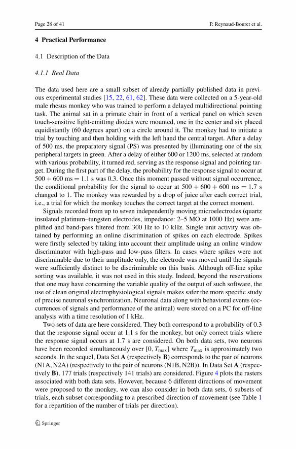
Two sets of data are here considered. They both correspond to a probability of 0.3that the response signal occur at 1.1 s for the monkey, but only correct trials wherethe response signal occurs at 1.7 s are considered. On both data sets, two neuronshave been recorded simultaneously over [0, Tmax] where Tmax is approximately twoseconds. In the sequel, Data Set A (respectively B) corresponds to the pair of neurons(N1A, N2A) (respectively to the pair of neurons (N1B, N2B)). In Data Set A (respec-tively B), 177 trials (respectively 141 trials) are considered. Figure 4 plots the rastersassociated with both data sets. However, because 6 different directions of movementwere proposed to the monkey, we can also consider in both data sets, 6 subsets oftrials, each subset corresponding to a prescribed direction of movement (see Table 1for a repartition of the number of trials per direction).

Journal of Mathematical Neuroscience (2014) 4:3 Page 29 of 41
Fig. 4 Raster plots of the data sets. In panel a the rasters associated to Data Set A i.e. (N1A, N2A). Inpanel b, the ones associated to Data Set B, i.e. (N1B, N2B). Each line corresponds to a trial, each dot to aspike
Table 1 Repartition of numberof trials on the real data sets Direction Total
1 2 3 4 5 6
Data Set A 28 31 30 35 28 25 177
Data Set B 23 24 26 18 30 20 141
Therefore, n, the total number of trials will be close to 200 if one aggregates overall the directions or will belong to the interval [20,35] if one considers the trialsaccording to the directions. Those trials are assumed to be i.i.d. This assumption ismore reasonable if one considers trials for a fixed given direction.
4.1.2 Simulated Data
To assess the performance of our procedure, simulated data for which the underly-ing model is known have also been simulated. Three different data sets have beensimulated, with the thinning method [63]:
• (S-HomPoi) Spikes are distributed according to an homogeneous Poisson pro-cesses of intensity 20 Hz on [0,2] s.
• (S-InPoi) Spikes are distributed according to an inhomogeneous Poisson processeswith piecewise continuous intensity on [0,2] s given by
t → λ(t) =3∑
i=1
[gi + hie
−4∗(t−ci )2/(r2
i −(t−ci )2)
]1t∈[ci−ri ;ci+ri ),
with g = [5,30,0], h = [12.5,15,12.5], c = [0.375,1.25,1.825], and r =[0.375,0.5,0.125].
• (S-Haw) Two spike trains are simulated according to a bivariate Hawkes processobserved on [0,2]. Each process is respectively denoted N(1) and N(2). Theirintensities are given by (17) with spontaneous parameters ν(1) = ν(2) = 20 Hz
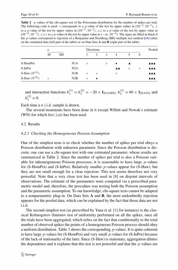
Page 30 of 41 P. Reynaud-Bouret et al.
Table 2 p-values of the chi-square test of the Poissonian distribution for the number of spikes per trial.The following code is used: ◦ corresponds to a p-value of the test by upper values in [10−2,10−1), �to a p-value of the test by upper values in [10−3,10−2), �� to a p-value of the test by upper value in[10−4,10−3), ��� to a p-value of the test by upper value in (−∞,10−4). The signs are filled in black ifthe p-values correspond to rejection of a Benjamini and Hochberg (BH) multiple test method [64] eitheron the simulated data (left part of the table) or on Data Sets A and B (right part of the table)
n Directions Pooled
40 200 1 2 3 4 5 6
S-HomPoi N1A ◦ ◦ • � ���S-InPoi N2A �� ◦ ◦ ���S-Haw (N(1)) N1B ◦ ◦ ◦ ���S-Haw (N(2)) ◦ N2B ◦ • ���
and interaction functions h(1)1 = h
(2)2 = −20 × 1[0,0.005], h
(1)2 = 60 × 1[0,0.01] and
h(2)1 = 0.
Each time a n i.i.d. sample is drawn.The several treatments have been done in R except Willett and Nowak’s estimate
(WN) for which Matlab has been used.
4.2 Results
4.2.1 Checking the Homogeneous Poisson Assumption
One of the simplest tests is to check whether the number of spikes per trial obeys aPoisson distribution with unknown parameter. Since the Poisson distribution is dis-crete, one can use a chi-square test with one estimated parameter, whose results aresummarized in Table 2. Since the number of spikes per trial is also a Poisson vari-able for inhomogeneous Poisson processes, it is reasonable to have large p-valuesfor (S-HomPoi) and (S-InPoi). Relatively smaller p-values appear for (S-Haw), butthey are not small enough for a clear rejection: This test seems therefore not verypowerful. Note that a very close test has been used in [8] on disjoint intervals ofobservations. The estimate of the parameters were computed via a prescribed para-metric model and, therefore, the procedure was testing both the Poisson assumptionand the parametric assumption. To our knowledge, chi-square tests cannot be adaptedto a nonparametric plug-in. On Data Sets A and B, the most undoubtedly rejectionappears for the pooled data, which can be explained by the fact that those data are noti.i.d.
The second simplest test (as prescribed by Yana et al. [1] for instance) is the clas-sical Kolmogorov–Smirnov test of uniformity performed on all the spikes, once allthe trials have been aggregated, which relies on the fact that conditionally to the totalnumber of observed spikes the points of a homogeneous Poisson process should obeya uniform distribution. Table 3 shows the corresponding p-values. It is quite coherentto have large p-values for (S-HomPoi) and very small p-values for (S-InPoi) becauseof the lack of stationarity of the later. Since (S-Haw) is stationary, aggregation dilutesthe dependence and it explains that this test is not powerful and that the p-values are

Journal of Mathematical Neuroscience (2014) 4:3 Page 31 of 41
Table 3 p-values of the classical K.S. test of uniformity on the spikes, all trials being aggregated. Samecodes as in Table 2. Note that none of the p-values were close enough to 1 to force a rejection by the testby lower values (i.e., rejection when the test statistic is smaller than kn,α , which corresponds to p-valuesof the test by upper values larger than 1 − α)
n Directions Pooled
40 200 1 2 3 4 5 6
S-HomPoi N1A ��� ��� ��� • ��� �� ���S-InPoi ��� ��� N2A ��� ��� ��� ��� ��� ��� ���S-Haw (N(1)) N1B ��� ��� ��� ��� ��� ��� ���S-Haw (N(2)) N2B ��� ��� ��� ��� ��� � ���
Table 4 p-values of Test 1 on the ISI, with a subsample size �[nISItot ]2/3�, where nISI
tot is the total numberof ISI that have been observed in all the trials. Same codes as in Table 2 for the p-values. Note that noneof the p-values were close enough to 1 to force a rejection by the test by lower values (i.e., rejection whenthe test statistic is smaller than kn,α , which corresponds to p-values of the test by upper values larger than1 − α)
n Directions Pooled
40 200 1 2 3 4 5 6
S-HomPoi N1A ��� ��� � • ◦ ���S-InPoi �� ��� N2A ��� ��� ��� � ��� ��� ���S-Haw (N(1)) ◦ � N1B ��� ��� ��� • ��� ��� ���S-Haw (N(2)) � ��� N2B • ��� � ◦ �� � ���
large in this case. This test clearly rejects for Data Sets A and B the homogeneousPoisson hypothesis.
Another test of first-order statistics as explained in [1] is the exponential test onthe ISI (see Table 4). Here, we apply our version of the exponential test, i.e., Test 1,using the subsampling scheme. As soon as there is enough trials, this test is power-ful enough to detect the nonstationarity (S-InPoi), but also the dependence (S-Haw),since there is no aggregation to dilute the dependence between consecutive points inone trial with respect to the previous test. On Data Sets A and B, the result is almostthe same as the previous test.
4.2.2 Checking the Inhomogeneous Poisson Assumption
Let us first look at the reconstructions of the underlying intensities. We first programtwo very basic kernel estimates (10): the sliding window (i.e., K = (1/2)1[−1,1])with length 0.1 s (i.e., bandwidth 0.05), denoted λ
SWhn , and the Gaussian kernel (used
for instance in [8]) with the same bandwidth and denoted λKhn . As [8], we also pro-
grammed a data-driven choice of bandwidth, called the thumb rule (here we followed[39] to construct it): it is denoted λ
Kh∗n . Finally, we programmed the three presented
adaptive method. The GL estimate, λGLn is programmed with the Gaussian kernel,
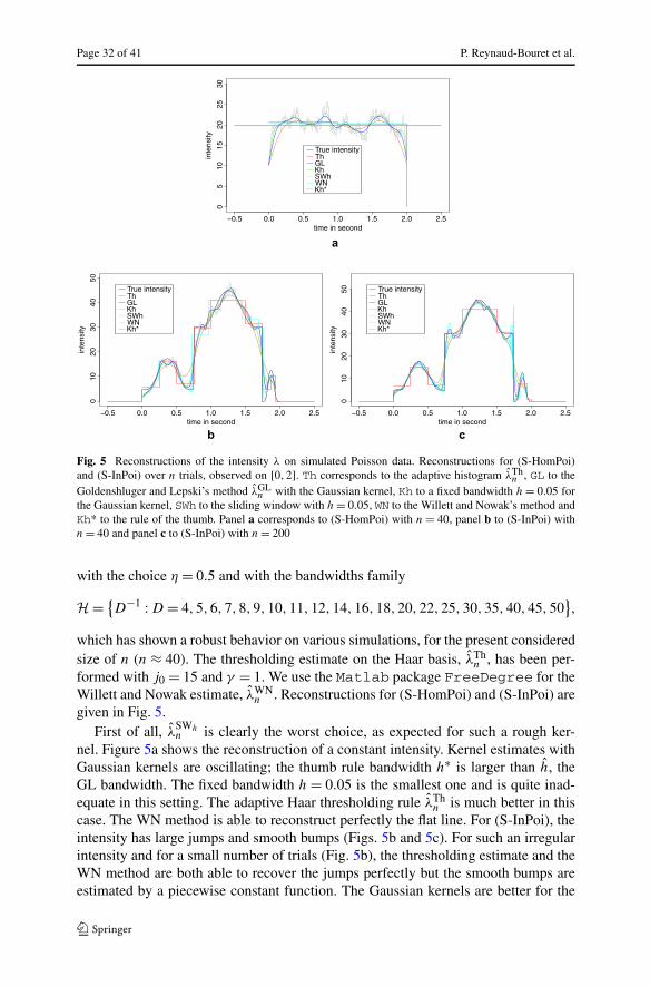
Page 32 of 41 P. Reynaud-Bouret et al.
Fig. 5 Reconstructions of the intensity λ on simulated Poisson data. Reconstructions for (S-HomPoi)and (S-InPoi) over n trials, observed on [0,2]. Th corresponds to the adaptive histogram λTh
n , GL to theGoldenshluger and Lepski’s method λGL
n with the Gaussian kernel, Kh to a fixed bandwidth h = 0.05 forthe Gaussian kernel, SWh to the sliding window with h = 0.05, WN to the Willett and Nowak’s method andKh* to the rule of the thumb. Panel a corresponds to (S-HomPoi) with n = 40, panel b to (S-InPoi) withn = 40 and panel c to (S-InPoi) with n = 200
with the choice η = 0.5 and with the bandwidths family
H = {D−1 : D = 4,5,6,7,8,9,10,11,12,14,16,18,20,22,25,30,35,40,45,50
},
which has shown a robust behavior on various simulations, for the present consideredsize of n (n ≈ 40). The thresholding estimate on the Haar basis, λTh
n , has been per-formed with j0 = 15 and γ = 1. We use the Matlab package FreeDegree for theWillett and Nowak estimate, λWN
n . Reconstructions for (S-HomPoi) and (S-InPoi) aregiven in Fig. 5.
First of all, λSWhn is clearly the worst choice, as expected for such a rough ker-
nel. Figure 5a shows the reconstruction of a constant intensity. Kernel estimates withGaussian kernels are oscillating; the thumb rule bandwidth h∗ is larger than h, theGL bandwidth. The fixed bandwidth h = 0.05 is the smallest one and is quite inad-equate in this setting. The adaptive Haar thresholding rule λTh
n is much better in thiscase. The WN method is able to reconstruct perfectly the flat line. For (S-InPoi), theintensity has large jumps and smooth bumps (Figs. 5b and 5c). For such an irregularintensity and for a small number of trials (Fig. 5b), the thresholding estimate and theWN method are both able to recover the jumps perfectly but the smooth bumps areestimated by a piecewise constant function. The Gaussian kernels are better for the
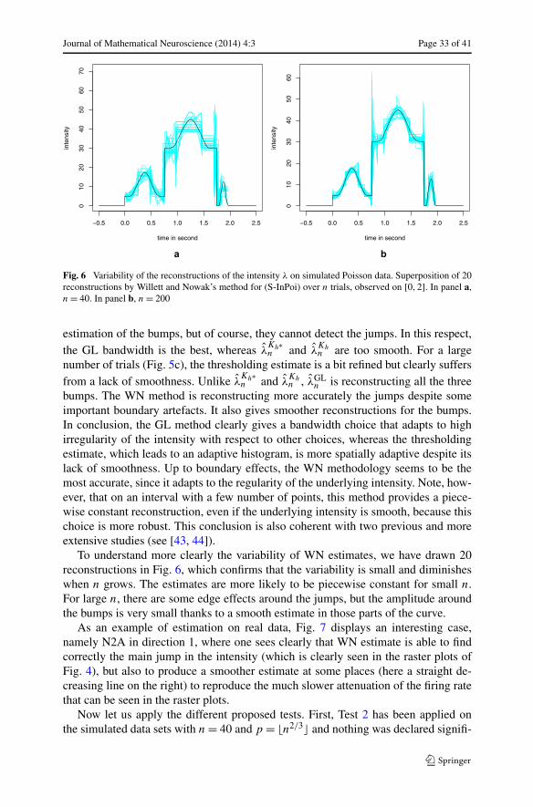
Journal of Mathematical Neuroscience (2014) 4:3 Page 33 of 41
Fig. 6 Variability of the reconstructions of the intensity λ on simulated Poisson data. Superposition of 20reconstructions by Willett and Nowak’s method for (S-InPoi) over n trials, observed on [0,2]. In panel a,n = 40. In panel b, n = 200
estimation of the bumps, but of course, they cannot detect the jumps. In this respect,the GL bandwidth is the best, whereas λ
Kh∗n and λ
Khn are too smooth. For a large
number of trials (Fig. 5c), the thresholding estimate is a bit refined but clearly suffersfrom a lack of smoothness. Unlike λ
Kh∗n and λ
Khn , λGL
n is reconstructing all the threebumps. The WN method is reconstructing more accurately the jumps despite someimportant boundary artefacts. It also gives smoother reconstructions for the bumps.In conclusion, the GL method clearly gives a bandwidth choice that adapts to highirregularity of the intensity with respect to other choices, whereas the thresholdingestimate, which leads to an adaptive histogram, is more spatially adaptive despite itslack of smoothness. Up to boundary effects, the WN methodology seems to be themost accurate, since it adapts to the regularity of the underlying intensity. Note, how-ever, that on an interval with a few number of points, this method provides a piece-wise constant reconstruction, even if the underlying intensity is smooth, because thischoice is more robust. This conclusion is also coherent with two previous and moreextensive studies (see [43, 44]).
To understand more clearly the variability of WN estimates, we have drawn 20reconstructions in Fig. 6, which confirms that the variability is small and diminisheswhen n grows. The estimates are more likely to be piecewise constant for small n.For large n, there are some edge effects around the jumps, but the amplitude aroundthe bumps is very small thanks to a smooth estimate in those parts of the curve.
As an example of estimation on real data, Fig. 7 displays an interesting case,namely N2A in direction 1, where one sees clearly that WN estimate is able to findcorrectly the main jump in the intensity (which is clearly seen in the raster plots ofFig. 4), but also to produce a smoother estimate at some places (here a straight de-creasing line on the right) to reproduce the much slower attenuation of the firing ratethat can be seen in the raster plots.
Now let us apply the different proposed tests. First, Test 2 has been applied onthe simulated data sets with n = 40 and p = �n2/3� and nothing was declared signifi-
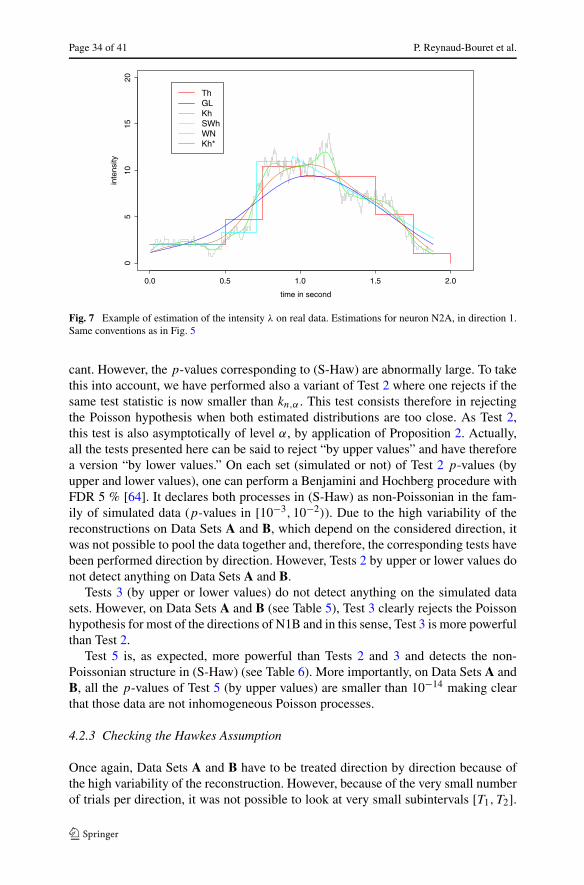
Page 34 of 41 P. Reynaud-Bouret et al.
Fig. 7 Example of estimation of the intensity λ on real data. Estimations for neuron N2A, in direction 1.Same conventions as in Fig. 5
cant. However, the p-values corresponding to (S-Haw) are abnormally large. To takethis into account, we have performed also a variant of Test 2 where one rejects if thesame test statistic is now smaller than kn,α . This test consists therefore in rejectingthe Poisson hypothesis when both estimated distributions are too close. As Test 2,this test is also asymptotically of level α, by application of Proposition 2. Actually,all the tests presented here can be said to reject “by upper values” and have thereforea version “by lower values.” On each set (simulated or not) of Test 2 p-values (byupper and lower values), one can perform a Benjamini and Hochberg procedure withFDR 5 % [64]. It declares both processes in (S-Haw) as non-Poissonian in the fam-ily of simulated data (p-values in [10−3,10−2)). Due to the high variability of thereconstructions on Data Sets A and B, which depend on the considered direction, itwas not possible to pool the data together and, therefore, the corresponding tests havebeen performed direction by direction. However, Tests 2 by upper or lower values donot detect anything on Data Sets A and B.
Tests 3 (by upper or lower values) do not detect anything on the simulated datasets. However, on Data Sets A and B (see Table 5), Test 3 clearly rejects the Poissonhypothesis for most of the directions of N1B and in this sense, Test 3 is more powerfulthan Test 2.
Test 5 is, as expected, more powerful than Tests 2 and 3 and detects the non-Poissonian structure in (S-Haw) (see Table 6). More importantly, on Data Sets A andB, all the p-values of Test 5 (by upper values) are smaller than 10−14 making clearthat those data are not inhomogeneous Poisson processes.
4.2.3 Checking the Hawkes Assumption
Once again, Data Sets A and B have to be treated direction by direction because ofthe high variability of the reconstruction. However, because of the very small numberof trials per direction, it was not possible to look at very small subintervals [T1, T2].
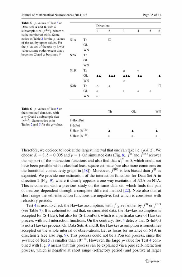
Journal of Mathematical Neuroscience (2014) 4:3 Page 35 of 41
Table 5 p-values of Test 3 onData Sets A and B, with asubsample size �n2/3�, where n
is the number of trials. Samecodes as Table 2 for the p-valuesof the test by upper values. Forthe p-values of the test by lowervalues, same codes except that ◦becomes � and � becomes �
Directions
1 2 3 4 5 6
N1A Th �GL
WN
N2A Th
GL
WN
N1B Th � ◦GL �� ��� ��� �� �WN �
N2B Th � ◦ �GL ◦ ◦ ◦ ◦WN ◦
Table 6 p-values of Test 5 onthe simulated data sets, withn = 40 and a subsample size�n2/3�. Same codes as inTables 2 and 5 for the p-values
Th GL WN
S-HomPoi
S-InPoi
S-Haw (N(1)) � � �S-Haw (N(2)) ◦ ◦ ◦
Therefore, we decided to look at the largest interval that one can take i.e. [Kδ,2]. Wechoose K = 8, δ = 0.005 and γ = 1. On simulated data (Fig. 8), f B and f BO recoverthe support of the interaction functions and also find that h
(2)1 = 0, which could not
have been possible with a classical least-square estimate (see also more comments onthe functional connectivity graph in [58]). Moreover, f BO is less biased than f B asexpected. We provide one estimation of the interaction functions for Data Set A indirection 2 (Fig. 9), where it clearly appears a one way excitation of N2A on N1A.This is coherent with a previous study on the same data set, which finds this pairof neurons dependent through a complete different method [22]. Note also that atshort range the self-interaction functions are negative, fact which is consistent withrefractory periods.
Test 4 is used to check the Hawkes assumption, with f given either by f B or f BO
(see Table 7). It is coherent to find that, on simulated data, the Hawkes assumption isaccepted for (S-Haw), but also for (S-HomPoi), which is a particular case of Hawkesprocess with null interaction functions. On the contrary, Test 4 detects that (S-InPoi)is not a Hawkes process. On Data Sets A and B, the Hawkes assumption is sometimesaccepted on the whole interval of observations. Let us focus for instance on N1A indirection 2 (see also Fig. 9). This process could not be a Poisson process, since thep-value of Test 5 is smaller than 10−14. However, the large p-value for Test 4 com-bined with Fig. 9 means that this process can be explained via a pure self-interactionprocess, which is negative at short range (refractory period) and positive at larger

Page 36 of 41 P. Reynaud-Bouret et al.
Fig. 8 Reconstruction of the interaction functions on simulated data. Reconstructions for (S-Haw) with
n = 40 trials, with T1 = 0.05 and T2 = 2. On the upper left, the interaction function h(1)1 , on the upper
right, h(1)2 , on the bottom left h
(2)1 and on the bottom right h
(2)2 . In black, the true interaction functions, in
green, reconstruction by method f B, in red, reconstruction by method f BO. On the top of each graphics,the true spontaneous parameter ν(1) on the top and the true parameter ν(2) on the bottom are referred byS*. The estimated spontaneous parameters by method f B are referred as SB and the estimated spontaneousparameters by method f BO are referred as SBO. We used K = 8, δ = 0.005, and γ = 1
range. Note that 9 processes on the 24 are not explained in this way (in particularN2A in direction 2), and are not Poisson either: Ihis can be due to a too large lack ofstationarity, combined with a large dependence between points.
5 Conclusion
When using the time-rescaling theorem to assess whether an observed spike trainobeys a certain probabilistic model (e.g., Poisson, Hawkes, etc.), a plug-in step iscurrently performed [1–3, 8, 24]. If this plug-in step is done without care the result-ing test may be much too conservative leading to poor detections (see Fig. 1). Wepropose here to use the subsampling as an almost universal solution when dealingwith Kolmogorov–Smirnov tests of uniformity, such a universal solution being com-pletely new. The main requirement is to have access to an estimate of the underlyingintensity, whose rate of convergence is known (see, for instance, (5)).
In classical previous works such as [8, 23], parametric estimates such as MLE overa prescribed parametric model are used as plug-in estimates, which are convergingtoward the true intensity when the underlying parametric model is true. Therefore,

Journal of Mathematical Neuroscience (2014) 4:3 Page 37 of 41
Fig. 9 Example of estimation of the interaction functions on real data. Estimations for Data Set A indirection 2 with n = 40 trials, with T1 = 0.05 and T2 = 2. Same conventions as in Fig. 8
Table 7 p-values of Test 4 with a subsample size �n2/3�. Same codes as in Tables 2 and 5 for the p-values
n = 40 Directions
1 2 3 4 5 6
S-HomPoi B N1A B ◦ ◦ ◦BO ◦ BO ��� ◦
S-InPoi B � N2A B ◦ �� � ◦BO BO ◦ ◦
S-Haw (N(1)) B N1B B � � ◦BO BO
S-Haw (N(2)) B N2B B ��� ��� ◦ �BO ◦ BO ◦ � �
when this parametric plug-in is used inside omnibus tests (and in particular the onespresented here), one has to be careful that we are not only testing the probabilis-tic assumption, but also the fact that the intensity belongs to the parametric model.To overcome this problem, we advertise for the use of nonparametric estimates andmore precisely to adaptive estimates, for which rates of convergence are known underlighter assumptions on the intensity than a prescribed parametric assumption. More-
Page 38 of 41 P. Reynaud-Bouret et al.
over, those adaptive methods have very good practical performance making them alsovery good in practice for estimation.
On some simulated data and on some real data sets, we have shown that ourmethod performs very well. However, there are still two main directions in whichour work need to be pursued in order to provide a more complete answer on real datasets. First of all, the KS test of exponentiality on the ISI can also be performed insteadof the KS test of uniformity [1]. If the method with subsampling can be adapted tothis case, we have presently no guarantee that this test would have a controlled level.Indeed we have no equivalent of Proposition 2 or Theorem 1 for the ISI repartition.The second main drawback is that we are clearly able to reject (at least on the pre-sented real data sets) both homogeneous and inhomogeneous Poisson assumptions.We are also able to test whether the processes are Hawkes or not, which in particulartakes into account refractory periods and dependence between several spike trains.However, the Hawkes model reflects stationary features, and cannot model nonsta-tionary data. Therefore, we would need a more general model, which includes thedependence as in the Hawkes model presented here, but also the non- stationarityas in the inhomogeneous Poisson process. At the present moment, models reflectingboth are not compatible with a full agnostic approach where no assumption is madeon the underlying functions, the estimation problem being not completely identifiable[16]. A first step will be therefore to provide a trade off between estimation capacityand not too restrictive assumptions on the process itself, with respect to real spiketrain data.
Competing Interests
The authors declare that they have no competing interests.
Authors’ Contributions
CTM is the main initiator of the project both from a theoretical and practical point of view and did most ofthe numerical experiments. PRB participated in both theoretical and practical aspects and did most of theredaction. VR participated in both theoretical aspects and redaction. FG highlighted the main questionsarising in neuroscience, thanks to his experience in this field.
Acknowledgements We are especially thankful to Alexa Riehle, leader of the Laboratory in which thedata used in this article were previously collected. The authors also wish to thank F. Picard for fruitfuldiscussions during several steps of this work. This research is partly supported by the French AgenceNationale de la Recherche (ANR 2011 BS01 010 01 projet Calibration) and by the PEPS BMI 2012-2013Estimation of dependence graphs for thalamo-cortical neurons and multivariate Hawkes processes.
References
1. Yana K, Takeuchi N, Takikawa Y, Shinomura M: A method for testing an extended Poisson hy-pothesis of spontaneous quantal transmitter release at neuromuscular junctions. Biophys J 1984,46(3):323-330.
2. Brown E, Barbieri R, Ventura V, Kass R, Frank L: The time rescaling theorem and its applicationto neural spike train analysis. Neural Comput 2002, 14(2):325-346.
3. Pouzat C, Chaffiol A: On goodness of fit tests for models of neuronal spike trains considered ascounting processes. Technical report; 2009. arXiv:0909.2785.

Journal of Mathematical Neuroscience (2014) 4:3 Page 39 of 41
4. Daley DJ, Vere-Jones D: An Introduction to the Theory of Point Processes. Volume I: ElementaryTheory and Methods. 2nd edition. New York: Springer; 2003. [Probability and Its Applications (NewYork).]
5. Pipa G, Grün S: Non-parametric significance estimation of joint-spike events by shuffling andresampling. Neurocomputing 2003, 52-54:31-37.
6. Pipa G, Diesmann M, Grün S: Significance of joint-spike events based on trial-shuffling by effi-cient combinatorial methods. Complexity 2003, 8(4):1-8.
7. Pouzat C, Chaffiol A: Automatic spike train analysis and report generation. An implementationwith R, R2HTML and STAR. J Neurosci Methods 2009, 181:119-144.
8. Ventura V, Carta R, Kass R, Gettner S, Olson C: Statistical analysis of temporal evolution in single-neuron firing rates. Biostatistics 2002, 3:1-20.
9. Dayan P, Abbott LF: Theoretical Neuroscience; 2011. [Computational Neuroscience.]10. Georgopoulos A, Schwartz A, Kettner R: Neuronal population coding of movement direction.
Science 1986, 233:1416-1419.11. Rizzolatti G, Craighero L: The mirror-neuron system. Annu Rev Neurosci 2004, 27:169-192.12. Shinomoto S: Estimating the firing rate. In Analysis of Parallel Spike Trains; 2010. [Springer Series
in Computational Neuroscience.]13. Grün S: Unitary Joint-Events in Multiple-Neuron Spiking Activity: Detection, Significance and Inter-
pretation. Thun: Verlag Harri Deutsch; 1996.14. Grün S, Diesmann M, Aertsen A: Unitary events analysis. In Analysis of Parallel Spike Trains; 2010.
[Springer Series in Computational Neuroscience.]15. Riehle A, Grammont F, Diesmann M, Grün S: Dynamical changes and temporal precision of syn-
chronised spiking activity in monkey motor cortex during movement preparation. J Physiol2000, 94:569-582.
16. Krumin M, Reutsky I, Shoham S: Correlation-based analysis and generation of multiple spiketrains using Hawkes models with an exogenous input. Front Comput Neurosci 2010, 4:147.
17. Pernice V, Staude B, Cardanobile S, Rotter S: How structure determines correlations in neuronalnetworks. PLoS Comput Biol 2012, 85:031916.
18. Pernice V, Staude B, Cardanobile S, Rotter S: Recurrent interactions in spiking networks witharbitrary topology. Phys Rev E, Stat Nonlinear Soft Matter Phys 2011, 7:e1002059.
19. Chornoboy E, Schramm L, Karr A: Maximum likelihood identification of neural point processsystems. Biol Cybern 1988, 59:265-275.
20. Pillow J, Shlens J, Paninski L, Sher A, Litke A, Chichilnisky E, Simoncelli E: Spatio-temporalcorrelations and visual signalling in a complete neuronal population. Nature 2008, 454:995-999.
21. Okatan M, Wilson M, Brown E: Analyzing functional connectivity using a network likelihoodmodel of ensemble neural spiking activity. Neural Comput 2005, 17:1927-1961.
22. Tuleau-Malot C, Rouis A, Grammont F, Reynaud-Bouret P: Multiple tests based on a Gaussianapproximation of the unitary events method. Technical report; 2012. http://hal.archives-ouvertes.fr/hal-00757323.
23. Ogata Y: Statistical models for earthquakes occurrences and residual analysis for point pro-cesses. J Am Stat Assoc 1988, 83(401):9-27.
24. Tuckwell H: Introduction to Theoretical Neurobiology. Volume 2: Nonlinear and Stochastic Theories;1988. [Cambridge Studies in Mathematical Biology.]
25. Barnard G: Time intervals between accidents—a note on Maguire, Pearson and Wynn’s paper.Biometrika 1953, 40(1/2):212-213.
26. Lawless J: Statistical Models and Methods for Lifetime Data. New York: Wiley-Interscience; 1982.27. Stephens M: EDF statistics for goodness of fit and some comparisons. J Am Stat Assoc 1974,
69(347):730-737.28. Bickel PJ, Doksum KA: Mathematical Statistics: Basic Ideas and Selected Topics. San Francisco:
Holden-Day; 1976. [Holden-Day Series in Probability and Statistics.]29. Andersen PK, Borgan Ø, Gill RD, Keiding N: Statistical Models Based on Counting Processes. New
York: Springer; 1993. [Springer Series in Statistics.]30. Shimazaki H, Shinomoto S: Kernel bandwidth optimization in spike rate estimation. J Comput
Neurosci 2010, 29:171-182.31. Brémaud P: Point Processes and Queues: Martingale Dynamics. New York: Springer; 1981. [Springer
Series in Statistics.]32. Papangelou F: Integrability of expected increments of point processes and a related random
change of scale. Trans Am Math Soc 1972, 165:483-506.
Page 40 of 41 P. Reynaud-Bouret et al.
33. Shorack GR, Wellner JA: Empirical Processes with Applications to Statistics. New York: Wiley; 1986.[Wiley Series in Probability and Mathematical Statistics: Probability and Mathematical Statistics.]
34. Hogg RV, Tanis EA: Probability and Statistical Inference. New York: Macmillan Co.; 1977.35. Roquain E: Type I error rate control in multiple testing: a survey with proofs. J. Soc. Fr. Stat.
2011, 152:3-38.36. Gerstein G, Perkel D: Simultaneous recorded trains of action potentials: analysis and functional
interpretation. Science 1969, 164:828-830.37. Tsybakov AB: Introduction to Nonparametric Estimation. New York: Springer; 2009. [Springer Se-
ries in Statistics.] Revised and extended from the 2004 French original, translated by Vladimir Zaiats.38. Rudemo M: Empirical choice of histograms and kernel density estimators. Scand J Stat 1982,
9(2):65-78.39. Silverman BW: Density Estimation for Statistics and Data Analysis. London: Chapman & Hall; 1986.
[Monographs on Statistics and Applied Probability.]40. Goldenshluger A, Lepski O: Bandwidth selection in kernel density estimation: oracle inequalities
and adaptive minimax optimality. Ann Stat 2011, 39(3):1608-1632.41. Reynaud-Bouret P: Adaptive estimation of the intensity of inhomogeneous Poisson processes via
concentration inequalities. Probab Theory Relat Fields 2003, 126:103-153.42. Rydén T: An EM algorithm for estimation in Markov-modulated Poisson processes. Comput Stat
Data Anal 1996, 21(4):431-447.43. Reynaud-Bouret P, Rivoirard V: Near optimal thresholding estimation of a Poisson intensity on
the real line. Electron J Stat 2010, 4:172-238.44. Reynaud-Bouret P, Rivoirard V, Tuleau-Malot C: Adaptive density estimation: a curse of support?
J Stat Plan Inference 2011, 141:115-139.45. Willett RM, Nowak RD: Multiscale Poisson intensity and density estimation. IEEE Trans Inf The-
ory 2007, 53(9):3171-3187.46. Perkel D, Gerstein G, Moore G: Neuronal spike trains and stochastic processes. II. Simultaneous
spike trains. Biophys J 1967, 7:419-440.47. Hawkes AG: Point spectra of some mutually exciting point processes. J R Stat Soc, Ser B 1971,
33:438-443.48. Gusto G, Schbath S: FADO: a statistical method to detect favored or avoided distances between
occurrences of motifs using the Hawkes’ model. Stat Appl Genet Mol Biol 2005, 4:24 (electronic).49. Carstensen L, Sandelin A, Winther O, Hansen N: Multivariate Hawkes process models of the oc-
currence of regulatory elements. BMC Bioinform 2010, 11:456.50. Brillinger D: The identification of point process systems. Ann Probab 1975, 3(6):909-924.51. Brillinger D, Bryant H, Segundo J: Identification of synaptic interactions. Biol Cybern 1976,
22:213-228.52. Brémaud P, Massoulié L: Stability of nonlinear Hawkes processes. Ann Probab 1996, 24(3):1563-
1588.53. Reynaud-Bouret P, Roy E: Some non asymptotic tail estimates for Hawkes processes. Bull Belg
Math Soc Simon Stevin 2007, 13(5):883-896.54. Vere-Jones D, Ozaki T: Some examples of statistical estimation applied to earthquake data. Ann
Inst Stat Math 1982, 34(B):189-207.55. Reynaud-Bouret P, Schbath S: Adaptive estimation for Hawkes processes; application to genome
analysis. Ann Stat 2010, 38(5):2781-2822.56. Blundell C, Heller K, Beck J: Modelling reciprocating relationships with Hawkes processes. In
Proceedings of NIPS; 2012.57. Hansen N, Reynaud-Bouret P, Rivoirard V: Lasso and probabilistic inequalities for multivariate
point processes. Bernoulli (to appear). arXiv:1208.0570.58. Reynaud-Bouret P, Rivoirard V, Tuleau-Malot C: Inference of functional connectivity in neuro-
sciences via Hawkes processes. In 1st IEEE Global Conference on Signal and Information Process-ing: Austin, Texas; 2013.
59. Aertsen A, Gerstein G, Habib M, Palm G: Dynamics of neuronal firing correlation: modulation of“effective connectivity”. J Neurophysiol 1989, 61(5):900-917.
60. Tibshirani R: Regression shrinkage and selection via the lasso. J R Stat Soc, Ser B 1996, 58:267-288.
61. Grammont F, Riehle A: Spike synchronisation and firing rate in a population of motor corticalneurons in relation to movement direction and reaction time. Biol Cybern 2003, 88:360-373.
62. Riehle A, Grammont F, MacKay A: Cancellation of a planned movement in monkey motor cortex.NeuroReport 2006, 17(3):281-285.

Journal of Mathematical Neuroscience (2014) 4:3 Page 41 of 41
63. Ogata Y: On Lewis’ simulation method for point processes. IEEE Trans Inf Theory 1981, 27:23-31.64. Benjamini Y, Hochberg Y: Controlling the false discovery rate: a practical and powerful approach
to multiple testing. J R Stat Soc, Ser B 1995, 57:289-300.