ChemicalScience

EDGE ARTICLE

Ope

n A

cces

s A

rtic

le. P

ublis

hed

on 1

2 O

ctob

er 2

021.

Dow

nloa

ded

on 2

/21/

2022

6:3

8:50

PM

. T

his

artic

le is

lice

nsed

und

er a

Cre

ativ

e C

omm

ons

Attr

ibut

ion

3.0

Unp

orte

d L

icen

ce.

View Article OnlineView Journal | View Issue

Golem: an algori

aVector Institute for Articial Intelligence,

aldeghi@vectorinstitute.ai; alan@aspuru.cobChemical Physics Theory Group, Departm

Toronto, ON, CanadacDepartment of Computer Science, UniversitdDepartment of Chemistry and Chemical Bio

USAeNational Research Council of Canada, OttafLebovic Fellow, Canadian Institute for Adva

† Electronic supplementary informa10.1039/d1sc01545a

Cite this: Chem. Sci., 2021, 12, 14792

All publication charges for this articlehave been paid for by the Royal Societyof Chemistry

Received 17th March 2021Accepted 11th October 2021

DOI: 10.1039/d1sc01545a

rsc.li/chemical-science

14792 | Chem. Sci., 2021, 12, 14792–1

thm for robust experiment andprocess optimization†

Matteo Aldeghi, *abc Florian Hase, abcd Riley J. Hickman, bc Isaac Tamblyn ae

and Alan Aspuru-Guzik *abcf

Numerous challenges in science and engineering can be framed as optimization tasks, including the

maximization of reaction yields, the optimization of molecular and materials properties, and the fine-

tuning of automated hardware protocols. Design of experiment and optimization algorithms are often

adopted to solve these tasks efficiently. Increasingly, these experiment planning strategies are coupled

with automated hardware to enable autonomous experimental platforms. The vast majority of the

strategies used, however, do not consider robustness against the variability of experiment and process

conditions. In fact, it is generally assumed that these parameters are exact and reproducible. Yet some

experiments may have considerable noise associated with some of their conditions, and process

parameters optimized under precise control may be applied in the future under variable operating

conditions. In either scenario, the optimal solutions found might not be robust against input variability,

affecting the reproducibility of results and returning suboptimal performance in practice. Here, we

introduce Golem, an algorithm that is agnostic to the choice of experiment planning strategy and that

enables robust experiment and process optimization. Golem identifies optimal solutions that are robust

to input uncertainty, thus ensuring the reproducible performance of optimized experimental protocols

and processes. It can be used to analyze the robustness of past experiments, or to guide experiment

planning algorithms toward robust solutions on the fly. We assess the performance and domain of

applicability of Golem through extensive benchmark studies and demonstrate its practical relevance by

optimizing an analytical chemistry protocol under the presence of significant noise in its experimental

conditions.

I. Introduction

Optimization problems, in which one seeks a set of parametersthat maximize or minimize an objective of interest, are ubiq-uitous across science and engineering. In chemistry, theseparameters may be the experimental conditions that control theyield of the reaction, or those that determine the cost-efficiencyof a manufacturing process (e.g., temperature, time, solvent,catalyst).1,2 The design of molecules and materials with specicproperties is also a multi-parameter, multi-objective optimiza-tion problem, with their chemical composition ultimately

Toronto, ON, Canada. E-mail: matteo.

m

ent of Chemistry, University of Toronto,

y of Toronto, Toronto, ON, Canada

logy, Harvard University, Cambridge, MA,

wa, ON, Canada

nced Research, Toronto, ON, Canada

tion (ESI) available. See DOI:

4807

governing their properties.3–7 These optimization tasks may, inprinciple, be performed autonomously. In fact, thanks to ever-growing automation, machine learning (ML)-driven experi-mentation has attracted considerable interest.8–14 Self-drivinglaboratories are already accelerating the rate at which theseproblems can be solved by combining automated hardware withML algorithms equipped with optimal decision-makingcapabilities.15–21

Recent efforts in algorithm development have focused onproviding solutions to the requirements that arise from thepractical application of self-driving laboratories. For instance,newly proposed algorithms include those with favorablecomputational scaling properties,22 with the ability to optimizemultiple objectives concurrently,23 that are able to handlecategorical variables (such as molecules) and integrate externalinformation into the optimization process.24 One practicalrequirement of self-driving laboratories that has received littleattention in this context is that of robustness against variabilityof experimental conditions and process parameters.

During an optimization campaign, it is typically assumedthat the experimental conditions are known and exactly repro-ducible. However, the hardware (e.g., dispensers, thermostats)

© 2021 The Author(s). Published by the Royal Society of Chemistry

Edge Article Chemical Science

Ope

n A

cces

s A

rtic

le. P

ublis

hed

on 1

2 O

ctob

er 2

021.

Dow

nloa

ded

on 2

/21/

2022

6:3

8:50

PM

. T

his

artic

le is

lice

nsed

und

er a

Cre

ativ

e C

omm

ons

Attr

ibut

ion

3.0

Unp

orte

d L

icen

ce.

View Article Online

may impose limitations on the precision of the experimentalprocedure such that there is a stochastic error associated withsome or all conditions. As a consequence, the optimal solutionfound might not be robust to perturbations of the inputs,affecting the reproducibility of the results and returningsuboptimal performance in practice. Another scenario is whena process optimized under precise control is to be adopted inthe future under looser operating conditions. For instance, inlarge-scale manufacturing, it might not be desirable (orpossible) to impose tight operating ranges on the processparameters due to the cost of achieving high precision. Thismeans that the tightly controlled input parameters used duringoptimization might not reect the true, variable operatingconditions that will be encountered in production.

In general, it is possible to identify two main types of inputvariability encountered in an experimental setting. The rst isdue to uncertainty in the experimental conditions that arecontrolled by the researchers, oen referred to as the controlfactors, corresponding to the examples discussed above. It canbe caused by the imprecision of the instrumentation, whichmay reect a fundamental limitation or a design choice, andcould affect the present or future executions of the experimentalprotocol. A second type of input variability that can affect theperformance of the optimization is due to experimental condi-tions that the researcher does not directly control. This may be,for instance, the temperature or the humidity of the room inwhich the experiments are being carried out. While it might notalways be possible or desirable to control these conditions, theymight be known and monitored such that their impact on theexperimental outcome can in principle be accounted for.25 Thework presented here focuses on the rst type of variability,related to control factors, although the approach presented maybe in principle extended and applied to environmental factorstoo.

Here, we introduce Golem, a probabilistic approach thatidenties optimal solutions that are robust to input uncertainty,thus ensuring the reproducible performance of optimizedexperiments and processes. Golem accounts for sources ofuncertainty and may be applied to reweight the merits ofprevious experiments, or integrated into popular optimizationalgorithms to directly guide the optimization toward robustsolutions. In fact, the approach is agnostic to the choice ofexperiment planning strategy and can be used in conjunctionwith both design of experiment and optimization algorithms.To achieve this, Golem explicitly models experimental uncer-tainty with suitable probability distributions that rene themerits of the collected measurements. This allows one to denean objective function that maximizes the average performanceunder variable conditions, while optionally also penalizing theexpected variance of the results.

The article is organized as follows. First, we review somebackground information and previous work on robust optimi-zation (Section II). Second, we introduce the core ideas behindthe Golem algorithm (Section III). We then present the analyt-ical benchmark functions used to test Golem together withdifferent optimization approaches (Section IV), as well as theresults of these benchmark studies (Section V). Finally, we show

© 2021 The Author(s). Published by the Royal Society of Chemistry

how Golem may be used in practice, taking the calibration ofa high-performance liquid chromatography (HPLC) protocol asan example application (Section VI).

II. Background and related work

Formally, an optimization task requires nding the set ofconditions x (i.e., the parameters, or control factors) that yield themost desirable outcome for f(x). If the most desirable outcomeis the one that minimizes f(x), then the solution of the optimi-zation problem is

x* ¼ arg minx˛X

f ðxÞ; (1)

where X is the domain of the optimization dening the range ofexperimental conditions that are feasible or that one is willingto consider. The objective function value f(x) determines themerit of a specic set of parameters x. This merit may reect theyield of a reaction, the cost-efficiency of a manufacturingprocess, or a property of interest for a molecule or material.Note that the objective function f(x) is a priori unknown, but canbe probed via experiment. Only a nite number K of samplesDK ¼ fx; f ðxÞgKk¼1 are typically collected during an optimizationcampaign, due to the cost and time of performing the experi-ments. A surrogate model of f(x) can be constructed based onDK: This model is typically a statistical or machine learning(ML) model that captures linear and non-linear relationshipsbetween the input conditions x and the objective functionvalues f(x).

An optimization campaign thus typically proceeds by itera-tively testing sets of parameters x, as dened via a design ofexperiment or as suggested by an experiment planning algo-rithm.26–28 Common design of experiment approaches rely onrandom or systematic searches of parameter combinations.Other experiment planning algorithms include sequentialmodel-based approaches, such as Bayesian optimization,29,30

and heuristic approaches like evolutionary and genetic algo-rithms.31–33 Experiment planning algorithms are now of partic-ular interest in the context of self-driving laboratories forchemistry and materials science,18,19,22,34,35 which aim to auton-omously and efficiently optimize the properties of moleculesand materials.

A. Robust optimization

The goal of robust optimization is to identify solutions to anoptimization problem that are robust to variation or sources ofuncertainty in the conditions under which the experiments areor will be performed.36 Robustness may be sought for differentreasons. For instance, the true location in parameter space ofthe query points being evaluated might be uncertain if experi-ments are carried out with imprecise instruments. In anotherscenario, a process might be developed in a tightly controlledexperimental setting, however, it is expected that future execu-tion of the same protocol will not. In such cases, a solution thatis insensitive to the variability of the experimental conditions isdesirable.

Chem. Sci., 2021, 12, 14792–14807 | 14793

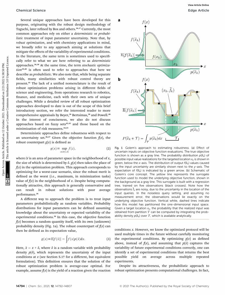
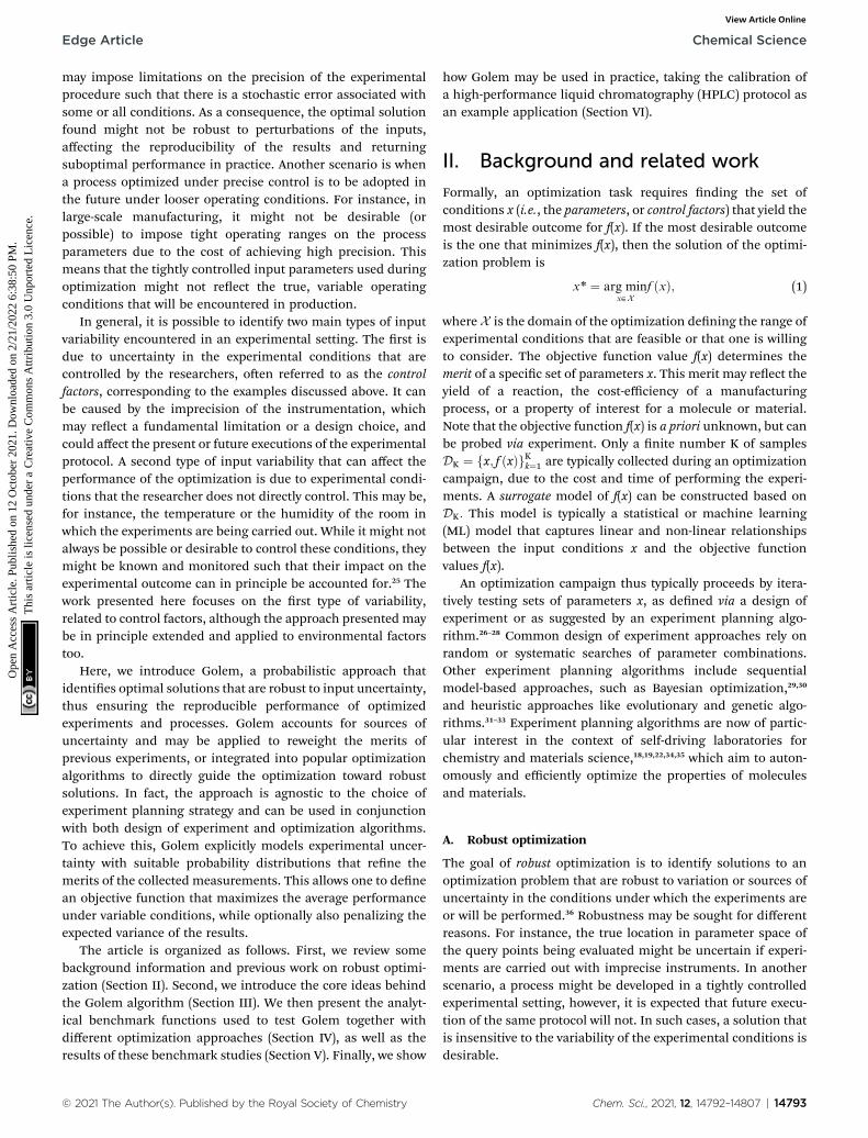
Fig. 1 Golem's approach to estimating robustness. (a) Effect ofuncertain inputs on objective function evaluations. The true objectivefunction is shown as a gray line. The probability distribution p(xk) ofpossible input value realizations for the targeted location xk is shown ingreen, below the x-axis. The distribution of output f(xk) values causedby the input uncertainty are similarly shown next to the y-axis. Theexpectation of f(xk) is indicated by a green arrow. (b) Schematic ofGolem's core concept. The yellow line represents the surrogatefunction used to model the underlying objective function, shown inthe background as a gray line. This surrogate is built with a regressiontree, trained on five observations (black crosses). Note how theobservations fk are noisy, due to the uncertainty in the location of theinput queries. In the noiseless query setting, and assuming nomeasurement error, the observations would lie exactly on theunderlying objective function. Vertical white, dashed lines indicatehow this model has partitioned the one-dimensional input space.Given a target location xk, the probability that the realized input wasobtained from partition T can be computed by integrating the prob-ability density p(xk) over T , which is available analytically.

Chemical Science Edge Article

Ope

n A

cces

s A

rtic

le. P

ublis

hed

on 1

2 O

ctob

er 2

021.

Dow

nloa

ded

on 2

/21/

2022

6:3

8:50

PM

. T

his

artic

le is

lice

nsed

und

er a

Cre

ativ

e C

omm

ons

Attr

ibut

ion

3.0

Unp

orte

d L

icen

ce.

View Article Online

Several unique approaches have been developed for thispurpose, originating with the robust design methodology ofTaguchi, later rened by Box and others.36,37 Currently, the mostcommon approaches rely on either a deterministic or probabi-listic treatment of input parameter uncertainty. Note that, byrobust optimization, and with chemistry applications in mind,we broadly refer to any approach aiming at solutions thatmitigate the effects of the variability of experimental conditions.In the literature, the same term is sometimes used to speci-cally refer to what we are here referring to as deterministicapproaches.36,38 At the same time, the term stochastic optimiza-tion39,40 is oen used to refer to approaches that here wedescribe as probabilistic. We also note that, while being separateelds, many similarities with robust control theory arepresent.41 The lack of a unied nomenclature is the result ofrobust optimization problems arising in different elds ofscience and engineering, from operations research to robotics,nance, and medicine, each with their own sets of uniquechallenges. While a detailed review of all robust optimizationapproaches developed to date is out of the scope of this briefintroductory section, we refer the interested reader to morecomprehensive appraisals by Beyer,36 Bertsimas,38 and Powell.40

In the interest of conciseness, we also do not discussapproaches based on fuzzy sets42,43 and those based on theminimization of risk measures.44,45

Deterministic approaches dene robustness with respect toan uncertainty set.46,47 Given the objective function f(x), therobust counterpart g(x) is dened as

gðxÞh supz˛Uðx;dÞ

f ðzÞ; (2)

where U is an area of parameter space in the neighborhood of x,the size of which is determined by d. g(x) then takes the place off(x) in the optimization problem. This approach corresponds tooptimizing for a worst-case scenario, since the robust merit isdened as the worst (i.e., maximum, in minimization tasks)value of f(x) in the neighborhood of x. Despite being computa-tionally attractive, this approach is generally conservative andcan result in robust solutions with poor averageperformance.36

A different way to approach the problem is to treat inputparameters probabilistically as random variables. Probabilitydistributions for input parameters can be dened assumingknowledge about the uncertainty or expected variability of theexperimental conditions.36 In this case, the objective functionf(x) becomes a random quantity itself, with its own (unknown)probability density (Fig. 1a). The robust counterpart of f(x) canthen be dened as its expectation value,

gðxÞhE½f ð~xÞ� ¼ðf ðxÞpð~xÞdx: (3)

Here, ~x ¼ x + d, where d is a random variable with probabilitydensity p(d), which represents the uncertainty of the inputconditions at x (see Section S.1† for a different, but equivalentformulation). This denition ensures that the solution of therobust optimization problem is average-case optimal. Forexample, assume f(x) is the yield of a reaction given the reaction

14794 | Chem. Sci., 2021, 12, 14792–14807

conditions x. However, we know the optimized protocol will beused multiple times in the future without carefully monitoringthe experimental conditions. By optimizing g(x) as denedabove, instead of f(x), and assuming that p(~x) captures thevariability of future experimental conditions correctly, one canidentify a set of experimental conditions that returns the bestpossible yield on average across multiple repeatedexperiments.

Despite its attractiveness, the probabilistic approach torobust optimization presents computational challenges. In fact,

© 2021 The Author(s). Published by the Royal Society of Chemistry

Edge Article Chemical Science

Ope

n A

cces

s A

rtic

le. P

ublis

hed

on 1

2 O

ctob

er 2

021.

Dow

nloa

ded

on 2

/21/

2022

6:3

8:50

PM

. T

his

artic

le is

lice

nsed

und

er a

Cre

ativ

e C

omm

ons

Attr

ibut

ion

3.0

Unp

orte

d L

icen

ce.

View Article Online

the above expectation cannot be computed analytically for mostcombinations of f(x) and p(~x). One solution is to approximateE½f ð~xÞ� by numerical integration, using quadrature or samplingapproaches.48–50 However, this strategy can become computa-tionally expensive as the dimensionality of the problemincreases and if g(x) is to be computed for many samples. As analternative numerical approach, it has been proposed to usea small number of carefully chosen points in x to cheaplyapproximate the integral.51 Selecting optimal points for arbi-trary probability distributions is not straightforward, however.52

In Bayesian optimization, it is common to use Gaussianprocess (GP) regression to build a surrogate model of theobjective function. A few approaches have been proposed in thiscontext to handle input uncertainty.53,54 Most recently, Frohlichet al.55 have introduced an acquisition function for GP-basedBayesian optimization for the identication of robust optima.This formulation is analytically intractable and the authorspropose two numerical approximation schemes. A similarapproach was previously proposed by Beland and Nair.56

However, in its traditional formulation, GP regression scalescubically with the number of samples collected. In practice, thismeans that optimizing g(x) can become costly aer collectingmore than a few hundred samples. In addition, GPs do notinherently handle discrete or categorical variables57 (e.g., type ofcatalyst), which are oen encountered in practical chemicalresearch. Finally, these approaches generally assume normallydistributed input noise, as this tends to simplify the problemformulation. However, physical constraints on the experimentalconditions may cause input uncertainty to deviate from thisscenario, such that it would be preferable to be able to modelany possible noise distribution.

In this work, we propose a simple, inexpensive, and exibleapproach to probabilistic robust optimization. Golem enablesthe accurate modeling of experimental conditions and theirvariability for continuous, discrete, and categorical conditions,and for any (parametric) bounded or unbounded uncertaintydistribution. By decoupling the estimation of the robustobjective g(x) from the details of the optimization algorithm,Golem can be used with any experiment planning strategy, fromdesign of experiment, to evolutionary and Bayesian optimiza-tion approaches.

III. Formulating golem

Consider a robust optimization problem in which the goal is tond a set of input conditions x˛X corresponding to the globalminimum of the function g : X/ℝ;

x* ¼ arg minx˛X

gðxÞ: (4)

We refer to g(x), as dened in eqn (3), as the robust objectivefunction, while noting that other integrated measures ofrobustness may also be dened.

Assume a sequential optimization in which we query a set ofconditions xk at each iteration k. If the input conditions arenoiseless, we can evaluate the objective function at xk (denotedfk). Aer K iterations, we will have built a dataset

© 2021 The Author(s). Published by the Royal Society of Chemistry

DK ¼ fxk; fkgKk¼1: However, if the input conditions are noisy, therealized conditions will be ~xk ¼ xk + d, where d is a randomvariable. As a consequence, we incur stochastic evaluations ofthe objective function, which we denote ~f k. This is illustrated inFig. 1a, where the Gaussian uncertainty in the inputs results ina broad distribution of possible output values. In this case, wewill have built a dataset ~D ¼ fxk; ~f kg

Kk¼1: Note that, while ~xk

generally refers to a random variable, when considered as partof a dataset ~D it may be interpreted as a specic sample of suchvariable. Hence, for added clarity, in Fig. 1 we refer to thedistributions on the y-axis as f(~xk), while we refer to functionevaluations on specic input values as ~f k.

A. General formalism

The goal of Golem is to provide a simple and efficient means toestimate g(x) from the available data, DK or ~DK: This wouldallow us to create a dataset GK ¼ fxk; gkgKk¼1 with robust merits,which can then be used to solve the robust optimization task ineqn (4). To do this, a surrogate model of the underlying objec-tive function f(x) is needed. This model should be able tocapture complex, non-linear relationships. In addition, itshould be computationally cheap to train and evaluate, and bescalable to high-data regimes. At the same time, we would liketo exibly model p(~x), such that it can satisfy physicalconstraints and closely approximate the true experimentaluncertainty. At the core of Golem is the simple observation thatwhen approximating f(x) with tree-based ML models, such asregression trees and random forest, estimates of g(x) can becomputed analytically as a nite series for any parametricprobability density p(~x). A detailed derivation can be found inSection S.1.†

An intuitive depiction of Golem is shown in Fig. 1b. Tree-based models are piece-wise constant and rely on the rectan-gular partitioning of input space. Because of this discretization,E½f ðxÞ� can be obtained as a constant contribution from eachpartition T , weighted by the probability of x being within eachpartition, Pðxk˛T Þ: Hence, an estimate of g(x) can be efficientlyobtained as a sum over all partitions (eqn (20)†).

Tree-based models such as regression trees and randomforests have a number of advantages that make them well-suited for this task. First, they are non-linear ML models thathave proved to be powerful function approximators. Second,they are fast to train and evaluate, adding little overhead to thecomputational protocols used. In the case of sequential opti-mization, the datasetDK grows at each iteration k, such that themodel needs to be continuously re-trained. Finally, they cannaturally handle continuous, discrete, and categorical variables,so that uncertainty in all type of input conditions can bemodeled. These reasons in addition to the fact that tree-basedmodels allow for a closed-form solution to eqn (3) makeGolem a simple yet effective approach for robust optimization.Note that while we decouple Golem's formulation from anyspecic optimization algorithm in this work, it is in principlepossible to integrate this approach into tree-ensemble Bayesianoptimization algorithms.58,59 This can be achieved via anacquisition function that is based on Golem's estimate of the

Chem. Sci., 2021, 12, 14792–14807 | 14795

Chemical Science Edge Article

Ope

n A

cces

s A

rtic

le. P

ublis

hed

on 1

2 O

ctob

er 2

021.

Dow

nloa

ded

on 2

/21/

2022

6:3

8:50

PM

. T

his

artic

le is

lice

nsed

und

er a

Cre

ativ

e C

omm

ons

Attr

ibut

ion

3.0

Unp

orte

d L

icen

ce.

View Article Online

robust objective, as well as its uncertainty, which can be esti-mated from the variance of g(x) across trees.

Fig. 2 shows a simple, one-dimensional example to provideintuition for Golem's behavior. In the top panel, the robustobjective function is shown for different levels of normally-distributed input noise, parameterized by the standard devia-tion s(x) reported. Note that, when there is no uncertainty ands(x) ¼ 0 (gray line), p(x) is a delta function and one recovers theoriginal objective function. As the uncertainty increases, theglobal minimum of the robust objective shis from being theone at x z 0.15 to that at x z 0.7. In the two panels at thebottom, the same effect is shown under a realistic low-datascenario, in which only a few observations of the objectivefunction are available (gray circles). Here, the dashed gray linerepresents the surrogate model used by Golem to estimate therobustness of each solution, given low (bottom le, greencircles) and high (bottom right, blue circles) input noise. As inthe top panel, which shows the continuous ground truth, heretoo the le-hand-side minimum is favored until the input noiseis large enough such that the right-hand-side minimumprovides better average-case performance.

Fig. 2 One-dimensional example illustrating the probabilisticapproach to robustness and Golem's behavior. The top panel showshow g(x), which is defined as E½f ðxÞ� ¼ Ð

f ðxÞpð~xÞdx; changes as thestandard deviation of normally-distributed input noise p(x) is increased.Note that the curve for s(x) ¼ 0 corresponds to the original objectivefunction. The panels at the bottom show the robust merits of a finiteset of samples as estimated by Golem from the objective functionvalues.

14796 | Chem. Sci., 2021, 12, 14792–14807

B. Multi-objective optimization

When experimental noise is present, optimizing for the robustobjective might not be the only goal. Oen, large variance in theoutcomes of an experimental procedure is undesirable, suchthat one might want to minimize it. For instance, in a chemicalmanufacturing scenario, one would like to ensure maximumoverall output across multiple plants and batches. However, itwould also be important that the amount of product manufac-tured in each batch does not vary considerably. Thus, theoptimal set of manufacturing conditions should not onlyprovide high yields on average, but also consistent ones. Theproblem can thus be framed as a multi-objective optimizationin which we would like to maximize E½f ðxÞ� while minimizing s

[f(x)] ¼ Var[f(x)]1/2. Golem can also estimate s[f(x)] (SectionS.1.D†), enabling such multi-objective optimizations. WithE½f ðxÞ� and s[f(x)] available, any scalarizing function may beused, including weighted sums and rank-based algorithms.23

IV. Benchmark surfaces and basicusage

The performance of Golem, in conjunction with a number ofpopular optimization algorithms, was evaluated on a set of two-dimensional analytical benchmark functions. This allowed usto test the performance of the approach under different, hypo-thetical scenarios, test which optimization algorithms are mostsuited to be combined with Golem, and demonstrate the waysin which Golem may be deployed.

A. Overview of the benchmark surfaces

Fig. 3 shows the benchmark functions that were used to eval-uate Golem. These benchmarks were chosen to both challengethe algorithm and show its exibility. We selected bothcontinuous and discrete surfaces, and bounded andunbounded probability distributions to describe the inputuncertainty. The objective functions considered are shown inthe second row of Fig. 3. The Bertsimas function is taken fromthe work of Bertsimas et al.,46 while Cliff and Sine are introducedin this work (Section S.2.A†). The rst row of Fig. 3 shows theuncertainty applied to these objective functions in both inputdimensions. These uncertainties induce the robust objectivefunctions shown in the third row. The location of the globalminimum is shown for each objective and robust objective,highlighting how the location of the global minimum is affectedby the variability of the inputs. The eight robust objectives in thethird row of Fig. 3 are labeled S1 to S8 and are the surfaces to beoptimized. While we can only probe the objective functions inthe second row, we use Golem to estimate their robust coun-terparts in the third row and locate their global minima.

These synthetic functions challenge Golem and the optimi-zation algorithms in different ways. The rougher the surfaceand its robust counterpart, the more challenging it is expectedto be to optimized. The smaller the difference in robust meritbetween the non-robust and robust minima (Section S.2.A,Table S1†), the harder it is for Golem to resolve the location ofthe true robust minimum, as more accurate estimates of g(x) are

© 2021 The Author(s). Published by the Royal Society of Chemistry

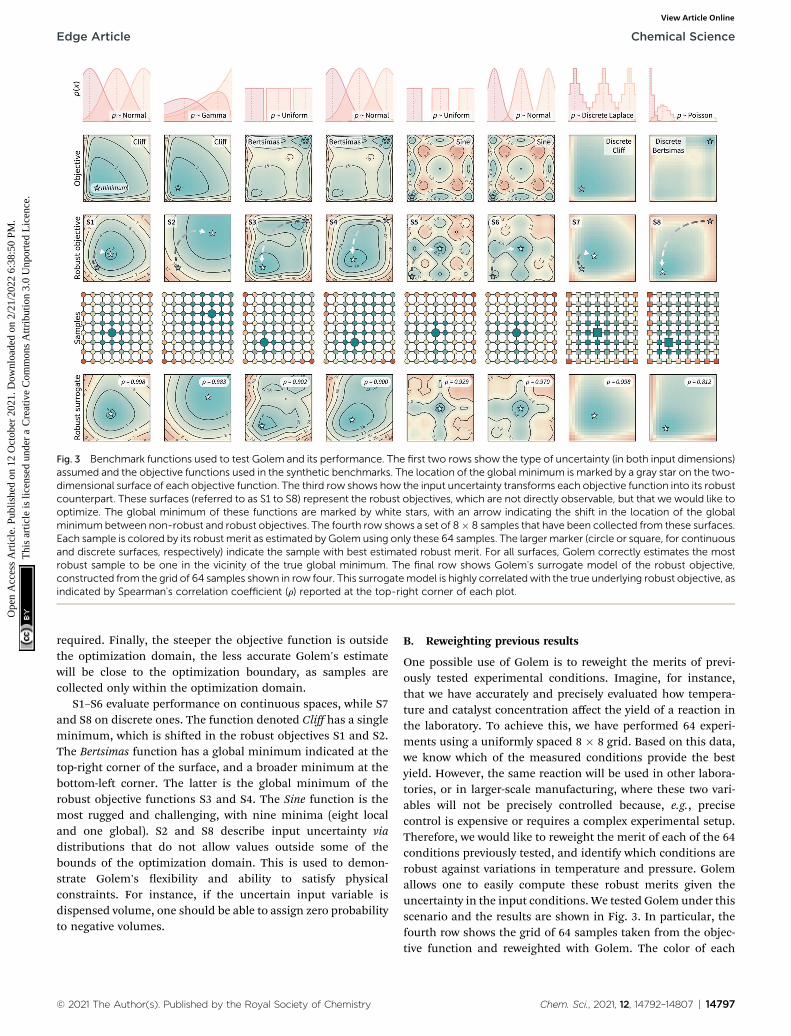
Fig. 3 Benchmark functions used to test Golem and its performance. The first two rows show the type of uncertainty (in both input dimensions)assumed and the objective functions used in the synthetic benchmarks. The location of the global minimum is marked by a gray star on the two-dimensional surface of each objective function. The third row shows how the input uncertainty transforms each objective function into its robustcounterpart. These surfaces (referred to as S1 to S8) represent the robust objectives, which are not directly observable, but that we would like tooptimize. The global minimum of these functions are marked by white stars, with an arrow indicating the shift in the location of the globalminimum between non-robust and robust objectives. The fourth row shows a set of 8� 8 samples that have been collected from these surfaces.Each sample is colored by its robust merit as estimated by Golem using only these 64 samples. The largermarker (circle or square, for continuousand discrete surfaces, respectively) indicate the sample with best estimated robust merit. For all surfaces, Golem correctly estimates the mostrobust sample to be one in the vicinity of the true global minimum. The final row shows Golem's surrogate model of the robust objective,constructed from the grid of 64 samples shown in row four. This surrogatemodel is highly correlatedwith the true underlying robust objective, asindicated by Spearman's correlation coefficient (r) reported at the top-right corner of each plot.

Edge Article Chemical Science

Ope

n A

cces

s A

rtic

le. P

ublis

hed

on 1

2 O

ctob

er 2

021.

Dow

nloa

ded

on 2

/21/

2022

6:3

8:50

PM

. T

his

artic

le is

lice

nsed

und

er a

Cre

ativ

e C

omm

ons

Attr

ibut

ion

3.0

Unp

orte

d L

icen

ce.

View Article Online

required. Finally, the steeper the objective function is outsidethe optimization domain, the less accurate Golem's estimatewill be close to the optimization boundary, as samples arecollected only within the optimization domain.

S1–S6 evaluate performance on continuous spaces, while S7and S8 on discrete ones. The function denoted Cliff has a singleminimum, which is shied in the robust objectives S1 and S2.The Bertsimas function has a global minimum indicated at thetop-right corner of the surface, and a broader minimum at thebottom-le corner. The latter is the global minimum of therobust objective functions S3 and S4. The Sine function is themost rugged and challenging, with nine minima (eight localand one global). S2 and S8 describe input uncertainty viadistributions that do not allow values outside some of thebounds of the optimization domain. This is used to demon-strate Golem's exibility and ability to satisfy physicalconstraints. For instance, if the uncertain input variable isdispensed volume, one should be able to assign zero probabilityto negative volumes.

© 2021 The Author(s). Published by the Royal Society of Chemistry

B. Reweighting previous results

One possible use of Golem is to reweight the merits of previ-ously tested experimental conditions. Imagine, for instance,that we have accurately and precisely evaluated how tempera-ture and catalyst concentration affect the yield of a reaction inthe laboratory. To achieve this, we have performed 64 experi-ments using a uniformly spaced 8 � 8 grid. Based on this data,we know which of the measured conditions provide the bestyield. However, the same reaction will be used in other labora-tories, or in larger-scale manufacturing, where these two vari-ables will not be precisely controlled because, e.g., precisecontrol is expensive or requires a complex experimental setup.Therefore, we would like to reweight the merit of each of the 64conditions previously tested, and identify which conditions arerobust against variations in temperature and pressure. Golemallows one to easily compute these robust merits given theuncertainty in the input conditions. We tested Golem under thisscenario and the results are shown in Fig. 3. In particular, thefourth row shows the grid of 64 samples taken from the objec-tive function and reweighted with Golem. The color of each

Chem. Sci., 2021, 12, 14792–14807 | 14797

Chemical Science Edge Article

Ope

n A

cces

s A

rtic

le. P

ublis

hed

on 1

2 O

ctob

er 2

021.

Dow

nloa

ded

on 2

/21/

2022

6:3

8:50

PM

. T

his

artic

le is

lice

nsed

und

er a

Cre

ativ

e C

omm

ons

Attr

ibut

ion

3.0

Unp

orte

d L

icen

ce.

View Article Online

sample indicates their robust merit as estimated by Golem, withblue being more robust and red less robust. The largest markerindicates the sample estimated to have the best robust merit,which is in close proximity to the location of the true robustminimum for all surfaces considered.

Based on these 64 samples, Golem can also build a surrogatemodel of the robust objective. This model is shown in the lastrow of Fig. 3. These estimates closely resemble the true robustsurfaces in the third row. In fact, the Spearman's rank correla-tions (r) between Golem's surrogates and the true robustobjectives were $0.9 for seven out of eight surfaces tested. ForS8 only, while the estimated location of the global robustminimum was still correct, r z 0.8 due to boundary effects. Infact, while the robust objective depends also on the behavior ofthe objective function outside of the dened optimizationdomain, we sample the objective only within this domain. Thislack of information causes the robustness estimates of pointsclose to the boundaries to be less accurate than for those fartherfrom them (Fig. S4†). Another consequence of this fact is thatthe robust surrogate does not exactly match the true robustobjective also in the limit of innite sampling within the opti-mization domain (Section S.2.B†).

To further clarify the above statement, by “dened optimi-zation domain” we refer to a subset of the physically-meaningful domain that the researcher has decided toconsider. Imagine, for instance, that we have a liquid dispenserwhich we will use to dispense a certain solvent volume. Thesmallest volume we can dispense is zero, while the largest mightbe the volume in the reservoir used (e.g., 1 L). These limits arephysical bounds we cannot exceed. However, for practicalpurposes, we will likely consider a maximum volume muchsmaller than the physical limit (e.g., 5 mL). In this example, 0–5 mL would constitute the dened optimization domain, while0–1 L are physical bounds on the domain. In the context ofuncertain experimental conditions, it can thus be the case thata noisy dispenser might provide 5.1 mL of liquid despite thisexceeding the desired optimization boundary. The samecannot, however, be the case for the lower bound in thisexample, since a negative volume is physically impossible. Asa consequence, while we allow an optimization algorithm toquery the objective function only within the user-dened opti-mization domain, a noisy experimental protocol might result inthe evaluation of the objective function outside of this domain.

Golem allows to take physical bounds into account bymodeling input uncertainty with bounded probability distri-butions. Yet, it cannot prevent boundary effects that are theconsequence of the unknown behaviour of the objective func-tion outside of the dened optimization domain. This issue,unfortunately, cannot be resolved in a general fashion, as itwould require a data-drivenmodel able to extrapolate arbitrarilyfar from the data used for training. A practical solution may beto consider a “data collection domain” as a superset of theoptimization domain, which is used for collecting data at theboundaries but which the optimization solution is not selectedfrom. In the examples in Fig. 3 (row 4), this would mean usingthe datapoints on the perimeter of the two-dimensional gridonly for estimating the robustness of the internal points more

14798 | Chem. Sci., 2021, 12, 14792–14807

accurately. We conclude by reiterating how, notwithstandingthis inescapable boundary effect, as shown in Fig. 3 there isa high correlation between Golem's estimates and the truerobustness values.

V. Optimization benchmarks

With increasing levels of automation and interest in self-drivinglaboratories, sequential approaches that make use of all datacollected to select the next, most informative experiment arebecoming the methods of choice for early prototypes of auton-omous science. In this case, rather than re-evaluating previouslyperformed experiments, one would like to steer the optimiza-tion towards robust solutions during the experimentalcampaign. Golem allows for this in combination with popularoptimization approaches, by mapping objective function eval-uations onto an estimate of their robust merits at each iterationof the optimization procedure. We evaluated the ability of sixdifferent optimization approaches to identify robust solutionswhen used with Golem and without. The algorithms testedinclude three Bayesian optimization approaches (Gryffin,22,24

GPyOpt,60 Hyperopt61), a genetic algorithm (Genetic),62 a randomsampler (Random), and a systematic search (Grid). Gryffin,GPyOpt, and Hyperopt use all previously collected data to decidewhich set of parameters to query next, Genetic uses part of thecollected data, while Random and Grid are totally agnostic toprevious measurements.

In these benchmarks, we allowed the algorithms to collect196 samples for continuous surfaces and 64 for the discreteones. We repeated each optimization 50 times to collect statis-tics. For Grid, we created a set of 14 � 14 uniformly-spacedsamples (8 � 8 for the discrete surfaces) and then selectedthem at random at each iteration. For all algorithms tested, weperformed the optimization with and without Golem. Algorithmperformance in the absence of Golem constitutes a naıvebaseline. Optimization performance in quantied usingnormalized cumulative robust regret, dened in S.2.C.† Thisregret is a relative measure of how fast each algorithm identiesincreasingly robust solutions, allowing the comparison ofalgorithm performance with respect to a specic benchmarkfunction.

A. Noiseless queries with uncertainty in future experiments

Here, we tested Golem under a scenario where queries duringthe optimization are deterministic, i.e., noiseless. It is assumedthat uncertainty in the inputs will arise only in future experi-ments. This scenario generally applies to the development ofexperimental protocols that are expected to be repeated underloose control of experimental conditions.

The results of the optimization benchmarks under thisscenario are summarized in Fig. 4, which shows the distribu-tions of cumulative regrets for all algorithms considered, withand without Golem, across the eight benchmark surfaces. Foreach algorithm, Fig. 4 also quanties the probability that theuse of Golem resulted in better performance in the identica-tion robust solutions. Overall, these results showed that Golem

© 2021 The Author(s). Published by the Royal Society of Chemistry

Fig. 4 Robust optimization performance of multiple algorithms, with and without Golem, in benchmarks where queries were noiseless. Boxplots show the distributions of cumulative regrets obtained across 50 optimization repeats with and without Golem, in purple and yellow,respectively. The boxes show the first, second, and third quartiles of the data, with whiskers extending up to 1.5 times the interquartile range. Atthe top of each plot, we report the probability that the use of Golem improved upon the performance of each algorithm. Probabilities are in greenif the performance with Golemwas significantly better (considering a 0.05 significance level) than without, and in red if it was significantly worse,as computed by bootstrap.

Edge Article Chemical Science

Ope

n A

cces

s A

rtic

le. P

ublis

hed

on 1

2 O

ctob

er 2

021.

Dow

nloa

ded

on 2

/21/

2022

6:3

8:50

PM

. T

his

artic

le is

lice

nsed

und

er a

Cre

ativ

e C

omm

ons

Attr

ibut

ion

3.0

Unp

orte

d L

icen

ce.

View Article Online

allowed the optimization algorithms to identify solutions thatwere more robust than those identied without Golem.

A few additional trends can be extracted from Fig. 4. TheBayesian optimization algorithms (Gryffin, GPyOpt, Hyperopt)and systematic searches (Grid) seemed to benet more from theuse of Golem than genetic algorithms (Genetic) and randomsearches (Random). In fact, the former approaches benetedfromGolem across all benchmark functions, while the latter didso only for half the benchmarks. The better performance of Gridas compared to Random, in particular, may appear surprising.We found that the main determinant of this difference is thefact that Grid samples the boundaries of the optimizationdomain, while Random is unlikely to do so. By forcing randomto sample the optimization boundaries, we recovered perfor-mances comparable to Grid (Section S.2.D†). We also hypothe-sized that uniformity of sampling might be benecial to Golem,given that the accuracy of the robustness estimate depends onhow well the objective function is modeled in the vicinity of theinput location considered. We indeed found that low-discrepancy sequences provided, in some cases, slightly betterperformance than random sampling. However, this effect wasminor compared to that of forcing the sampling of the opti-mization domain boundaries (Section S.2.D†).

Genetic likely suffered from the same pathology, given it isinitialized with random samples. Thus, in this context, initial-ization with a gridmay bemore appropriate. Genetic algorithmsare also likely to suffer from a second effect. Given that we canonly estimate the robust objective, Golem induces a history-

© 2021 The Author(s). Published by the Royal Society of Chemistry

dependent objective function. Contrary to Bayesian optimiza-tion approaches, genetic algorithms consider only a subset ofthe data collected during optimization, as they discard solu-tions with bad tness. Given that the robustness estimateschange during the course of the optimization, these algorithmsmay drop promising solutions early in the search, which arethen not recovered in the latter stages when Golem would havemore accurately estimated their robustness. The use of morecomplex genetic algorithm formulations, exploring a morediverse set of possible solutions,63 could improve this scenarioand is a possibility le for future work.

B. Noisy queries with uncertainty in current experiments

In a second scenario, queries during the optimization arestochastic, i.e., noisy, due the presence of substantial uncer-tainty in the current experimental conditions. This case appliesto any optimization campaign in which it is not possible toprecisely control the experimental conditions. However, weassume one can model the uncertainty p(~x), at least approxi-mately. For instance, this uncertainty might be caused by someapparatus (e.g., a solid dispenser) that is imprecise, but can becalibrated and the resulting uncertainty quantied. The opti-mization performances of the algorithms considered, with andwithout Golem, are shown in Fig. 5. Note that, to model therobust objective exactly, p(~x) should also be known exactly.While this is not a necessary assumption of the approach, theaccuracy of Golem's estimates is proportional to the accuracy ofthe p(~x) estimates. As the p(~x) estimate provided to Golem

Chem. Sci., 2021, 12, 14792–14807 | 14799

Fig. 5 Robust optimization performance of multiple algorithms, with and without Golem, in benchmarks where queries were noisy. Box plotsshow the distributions of cumulative regrets obtained across 50 optimization repeats with and without Golem, in purple and yellow, respectively.The boxes show the first, second, and third quartiles of the data, with whiskers extending up to 1.5 times the interquartile range. At the top of eachplot, we report the probability that the use of Golem improved the performance of each algorithm. Probabilities are in green if the performancewith Golem was significantly better (considering a 0.05 significance level) than without, and in red if it was significantly worse, as computed bybootstrap.

Chemical Science Edge Article

Ope

n A

cces

s A

rtic

le. P

ublis

hed

on 1

2 O

ctob

er 2

021.

Dow

nloa

ded

on 2

/21/

2022

6:3

8:50

PM

. T

his

artic

le is

lice

nsed

und

er a

Cre

ativ

e C

omm

ons

Attr

ibut

ion

3.0

Unp

orte

d L

icen

ce.

View Article Online

deviates from its true values, Golem under- or over-estimate therobustness of the optimal solution, depending on whether theinput uncertainty is under- or over-estimated. We will illustratethis point in more detail in Section VI.A.

Generally speaking, this is a more challenging scenario thanwhen queries are noiseless. As a consequence of the noisyexperimental conditions, the dataset collected does notcorrectly match the realized control factors x with their associ-ated merit f(x). Hence, the surrogate model is likely to bea worse approximation of the underlying objective functionthan when queries are noiseless. While the development of MLmodels capable of recovering the objective function f(x) basedon noisy queries ~x is outside the scope of this work, suchmodelsmay enable even more accurate estimates of robustness withGolem. We are not aware of approaches capable of performingsuch an operation, but it is a promising direction for futureresearch. In fact, being able to recover the (noiseless) objectivefunction from a small number of noisy samples ~f would bebenecial not only for robustness estimation, but for theinterpretation of experimental data more broadly.

Because of the above-mentioned challenge in the construc-tion of an accurate surrogate model, in some cases, theadvantage of using Golem might not seem as stark as in thenoiseless setting. This effect may be seen in surfaces S1 and S2,where the separation of the cumulative regret distributions islarger in Fig. 4 than it is in Fig. 5. Nonetheless, across allbenchmark functions and algorithms considered, the use of

14800 | Chem. Sci., 2021, 12, 14792–14807

Golem was benecial in the identication of robust solutions inthe majority of cases, and never detrimental, as shown by Fig. 5.In fact, Golem appears to be able to recover signicant corre-lations with the true robust objectives g(x) even when correla-tion with the objective functions f(x) is lost due to noise thequeried locations (Fig. S6†).

Optimization with noisy conditions is signicantly morechallenging than traditional optimization tasks with no inputuncertainty. However, the synthetic benchmarks carried outsuggest that Golem is able to efficiently guide optimizationcampaigns towards robust solutions. For example, Fig. 6 showsthe location of the best input conditions as identied by GPyOptwith and without Golem. Given the signicant noise present,without Golem, the optima identied by different repeatedexperiments are scattered far away from the robust minimum.When Golem is used, the optima identied are considerablymore clustered around the robust minimum.

C. Effect of forest size and higher input dimensions

All results shown thus far were obtained using a single regres-sion tree as Golem's surrogate model. However, Golem can alsouse tree-ensemble approaches, such as random forest64 andextremely randomized trees.65 We thus repeated the syntheticbenchmarks discussed above using these two ML models, withforest sizes of 10, 20, and 50 (Section S.2.F†). Overall, for thesetwo-dimensional benchmarks we did not observe signicantimprovements when using larger forest sizes. For the

© 2021 The Author(s). Published by the Royal Society of Chemistry

Fig. 6 Location of the optimal input parameters identified with andwithout Golem. The results shown were obtained with GPyOpt as theoptimization algorithm. A pink star indicates the location of the truerobust minimum. White crosses (one per optimization repeat, fora total of 50) indicate the locations of the optimal conditions identifiedby the algorithm without (on the left) and with (on the right) Golem.

Edge Article Chemical Science

Ope

n A

cces

s A

rtic

le. P

ublis

hed

on 1

2 O

ctob

er 2

021.

Dow

nloa

ded

on 2

/21/

2022

6:3

8:50

PM

. T

his

artic

le is

lice

nsed

und

er a

Cre

ativ

e C

omm

ons

Attr

ibut

ion

3.0

Unp

orte

d L

icen

ce.

View Article Online

benchmarks in the noiseless setting, regression trees appearedto provide slightly better performance against the Bertsimasfunctions (Fig. S7†). The lack of regularization may haveprovided a small advantage in this case, where Golem is tryingto resolve subtle differences between competing minima. Yet,a single regression tree performed as well as ensembles. For thebenchmarks in the noisy setting, random forest and extremelyrandomized trees performed slightly better overall (Fig. S8†).However, larger forests did not appear to provide considerableadvantage over smaller ones, suggesting that for these low-dimensional problems, small forests or even single trees cangenerally be sufficient.

To study the performance of different tree-ensembleapproaches also on higher-dimensional search spaces, weconducted experiments, similar to the ones described above, onthree-, four-, ve, and six-dimensional versions of benchmarksurface S1. In these tests, we consider two dimensions to beuncertain, while the additional dimensions are noiseless. Here,too, we studied the effect of forest type and size on the results,but we focused on the Bayesian optimization algorithms. In thiscase, we observed better performance of Golem when using

© 2021 The Author(s). Published by the Royal Society of Chemistry

random forest or extremely randomized trees as the surrogatemodel. In the noiseless setting, extremely randomized treesreturned slightly better performance than random forest, inparticular for GPyOpt and Hyperopt (Fig. S9†). The correlation ofoptimization performance with forest size was weaker. Yet, foreach combination of optimization algorithms and benchmarksurface, the best overall performance was typically achievedwith larger forest sizes of 20 or 50 trees. While less marked,similar trends were observed for the same tests in the noisysetting (Fig. S10†). In this scenario, random forest returnedslightly better performance than extremely randomized trees forHyperopt. Overall, surrogate models based on random forest orextremely randomized trees appear to provide better perfor-mance across different scenarios.

We then investigated Golem's performance across varyingsearch space dimensionality and number of uncertain condi-tions. To do this, we conducted experiments on three-, four-,ve, and six-dimensional versions of benchmark surface S1,with one to six uncertain inputs. These tests showed that Golemwas still able to guide the optimizations towards better robustsolutions. In the noiseless setting, the performance of GPyOptand Hyperopt was signicantly better with Golem for alldimensions and number of uncertain variables tested(Fig. S11†). The performance of Gryffin was signicantlyimproved by Golem in roughly half of the cases. Overall, givena certain search space dimensionality, the positive effect ofGolem becamemore marked with a higher number of uncertaininputs. This observation does not imply that the optimizationtask is easier with more uncertain inputs (it is in fact morechallenging), but that the use of Golem provides a moresignicant advantage in such scenarios. On the contrary, givena specic number of uncertain inputs, the effect of Golem wasless evident with increasing number of input dimensions.Indeed, additional input dimensions make it more challengingfor Golem to resolve whether the observed variability in theobjective function evaluations is due to the uncertain variablesor the expected behavior of the objective function along theadditional dimensions. Similar overall results were observed inthe noisy input setting (Fig. S12†). However, statisticallysignicant improvements were found in a smaller fraction ofcases. Here, we did not observe a signicant benet in usingGolem when having a small (1–2) number of uncertain inputs,but this became more evident with a larger (3–6) number ofuncertain inputs. In fact, the same trends with respect to thedimensionality of the search space and the number of uncertaininputs were observed also in the noisy query setting. Oneimportant observation is that Golem was almost never (one outof 108 tests) found to be detrimental to optimization perfor-mance, suggesting that there is very little risk in using theapproach when input uncertainty is present, as in the worst-case scenario Golem would simply leave the performance ofthe optimization algorithm used unaltered.

Overall, these results suggest that Golem is also effective onhigher-dimensional surfaces. In addition, it was found that theuse of surrogate models based on forests can, in some cases,provide a better optimization performance. Given the limitedcomputational cost of Golem, we thus generally recommend the

Chem. Sci., 2021, 12, 14792–14807 | 14801

Chemical Science Edge Article

Ope

n A

cces

s A

rtic

le. P

ublis

hed

on 1

2 O

ctob

er 2

021.

Dow

nloa

ded

on 2

/21/

2022

6:3

8:50

PM

. T

his

artic

le is

lice

nsed

und

er a

Cre

ativ

e C

omm

ons

Attr

ibut

ion

3.0

Unp

orte

d L

icen

ce.

View Article Online

use of an ensemble tree method as the surrogate model. Forestsizes of 20 to 50 trees were found to be effective. Yet, given thatlarger ensembles will not negatively affect the estimatorperformance, and that the runtime scales linearly with thenumber of trees, larger forests may be used as well.

VI. Chemistry applications

In this section, we provide an example application of Golem inchemistry. Specically, we consider the calibration of an HPLCprotocol, in which six controllable parameters (Fig. 7a, SectionS.3†) can be varied to maximize the peak area, i.e., the amountof drawn sample reaching the detector.26,66 Imagine we ran 1386experiments in which we tested combinations of these sixparameters at random. The experiment with the largest peakarea provides the best set of parameters found. The parametervalues corresponding to this optimum are highlighted in Fig. 7bby a gray triangle pointing towards the abscissa. With thecollected data, we can build a surrogate model of the responsesurface. The one shown as a gray line in Fig. 7b was built with200 extremely randomized trees.65 Fig. 7b shows the predictedpeak area when varying each of the six controllable parametersindependently around the optimum identied.

Fig. 7 Analysis of the robustness of an HPLC calibration protocol. (a)Flow path for the HPLC sampling sequence performed by a roboticplatform. The six parameters (P1–P6) are color coded. The yellowshade highlights the arm valve, and the gray shade the HPLC valve. (b)Golem analysis of the effect of input noise on expected protocolperformance. A surrogate model of the response surface is shown ingray. Uncertainties were modeled with truncated normal distributionswith standard deviations of 10%, 20%, 30% of each parameter's range.The corresponding robust surrogate models are shown in light green,dark green, and blue. Triangular markers and dashed lines indicate thelocation of the optima for each parameter under different levels ofnoise.

A. Analysis of prior experimental results

Golem allows us to speculate how the expected performance ofthis HPLC protocol would be affected by varying levels of noisein the controllable parameters. We modeled input noise viatruncated normal distributions that do not support valuesbelow zero. This choice satises the physical constraints of theexperiment, given that negative volumes, ows, and times arenot possible. We considered relative uncertainties correspond-ing to a standard deviation of 10%, 20%, and 30% of theallowed range for each input parameter. The protocol perfor-mance is most affected by uncertainty in the tubing volume(variable P3, Fig. 7b). A relative noise of 10% would result in anaverage peak area of around 1500 a.u., a signicant drop fromthe maximum observed at over 2000. It follows that to achieveconsistent high performance with this protocol, efforts shouldbe spent in improving the precision of this variable.

While the protocol performance (i.e., expected peak area) isleast robust against uncertainty in P3, the location of theoptimum setting for P3 is not particularly affected. Presence ofnoise in the sample loop (variable P1) has a larger effect on thelocation of its optimal settings. In fact, noise in P1 requireslarger volumes to be drawn into the sample loop to be able toachieve average optimal responses. The optimal parametersettings for the push speed (P5) and wait time (P6) are alsoaffected by the presence of noise. However, the protocolperformance is fairly insensitive to changes in these variables,with expected peak areas of around 2000 a.u. for any of theirvalues within the range studied.

Fig. 7 also illustrates the effect of under- or over-estimatingexperimental condition uncertainty on Golem's robustnessestimates. Imagine that the true uncertainty in variable P3 is20%. This may be the true uncertainty encountered in the future

14802 | Chem. Sci., 2021, 12, 14792–14807

deployment of the protocol, or it may be the uncertaintyencountered while trying to optimize it. If we assume, incor-rectly, the uncertainty to be 10%, Golem will predict theprotocol to return, on average, an area of �1500 a.u., while wewill nd that the true average performance of the protocolprovides an area slightly above 1000 a.u. That is, Golem willoverestimate the robustness of the protocol. On the other hand,

© 2021 The Author(s). Published by the Royal Society of Chemistry

Edge Article Chemical Science

Ope

n A

cces

s A

rtic

le. P

ublis

hed

on 1

2 O

ctob

er 2

021.

Dow

nloa

ded

on 2

/21/

2022

6:3

8:50

PM

. T

his

artic

le is

lice

nsed

und

er a

Cre

ativ

e C

omm

ons

Attr

ibut

ion

3.0

Unp

orte

d L

icen

ce.

View Article Online

if we assumed the uncertainty to be 30%, we would underestimatethe robustness of the protocol, as we would expect an average areabelow 1000 a.u. In the case of variable P3, however, the location ofthe optimum is only slightly affected by uncertainty, such thatdespite the incorrect prediction, Golem would still accuratelyidentify the location of the global optimum. That is, a tubingvolume of�0.3mL provides the best average outcome whether thetrue uncertainty is 10%, 20%, or 30%. In fact, while ignoringuncertainty altogether (i.e. assuming 0% uncertainty) would resultin the largest overestimate of robustness, it would still haveminimal impact in practice given that the prediction of theoptimum location would still be accurate. This is not the case if weconsidered P1. If we again assume that the true uncertainty in thisvariable is 20%, providing Golem with an uncertainty model with10% standard deviation would result in a protocol using a sampleloop volume of �0.04 mL, while the optimal one should be �0.06mL. Providing Golem with a 30% uncertainty instead would resultin an underestimate of the protocol robustness and an unneces-sarily conservative choice of�0.08 mL as the sample loop volume.

In summary, as anticipated in Section V.B, while anapproximate estimate of p(~x) does not prevent the use of Golem,it can affect the quality of its predictions. When uncertainty isunderestimated, the optimization solutions identied by Golemwill tend to be less robust than expected. On the contrary, whenuncertainty is overestimated, Golem's solutions will tend to beoverly conservative (i.e., Golem will favor plateaus in theobjective function despite more peaked optima would providebetter average performance). The errors in Golem's estimateswill be proportional to the error in the estimates of the inputuncertainty provided to it, but the magnitude of these errors isdifficult to predict as it depends on the objective function,which is unknown and application-specic. Note that, ignoringinput uncertainty corresponds to assuming p(~x) is a deltafunction in Golem. This choice, whether implicitly or explicitlymade, results in the largest possible overestimate of robustnesswhen uncertainty is in fact present. The associated error in theexpected robustness is likely to be small when the true uncer-tainty is small, but may be large otherwise.

It is important to note that, above, we analyzed only one-dimensional slices of the six-dimensional parameter space.Given interactions between these parameters, noise in oneparameter can affect the optimal setting of a different one(Section S.3.B†). Golem can identify these effects by studying itsmulti-dimensional robust surrogate model. Furthermore, forsimplicity, here we considered noise in each of the six control-lable parameters one at a time. It is nevertheless possible toconsider concurrent noise in as many parameters as desired.

This example shows how Golemmay be used to analyze priorexperimental results and study the effect of input noise onprotocol performance and the optimal setting of its controllableparameters.

B. Optimization of a noisy HPLC protocol

As a realistic and challenging example, we consider the opti-mization of the aforementioned HPLC sampling protocol underthe presence of signicant noise in P1 and P3 (noisy query

© 2021 The Author(s). Published by the Royal Society of Chemistry

setting). In this rst instance, we assume that the other condi-tions contain little noise and can thus be approximated asnoiseless. As before, we consider normally distributed noise,truncated at zero. We assume a standard deviation of 0.008 mLfor P1, and 0.08 mL for P3. In this example, we assume we areaware of the presence of input noise in these parameters, andare interested in achieving a protocol that returns an expectedpeak area, E½area�; of at least 1000 a.u. As a secondary objective,we would like to minimize the output variability, s[area], asmuch as possible while maintaining E½area�. 1000 a:u:

To achieve the optimization goals, we use Golem to estimateboth E½area� and s[area] as the optimization proceeds (Fig. 8a).We then use Chimera23 to scalarize these two objectives intoa single robust and multi-objective function, g[area], to beoptimized. Chimera is a scalarizing function that enables multi-objective optimization via the denition of a hierarchy ofobjectives and associated target values. As opposed to the post-hoc analysis discussed in the previous section, in this examplewe start with no prior experiment being available and let theoptimization algorithm request new experiments in order toidentify a suitable protocol. Here we perform virtual HPLC runsusing Olympus,26 which allows to simulate experiments viaBayesian Neural Network models. These probabilistic modelscapture the stochastic nature of experiments, such that theyreturn slightly different outcomes every time an experiment issimulated. In other words, they simulate the heteroskedasticnoise present in the experimental measurements. Whilemeasurement noise is not the focus of this work, it is anothersource of uncertainty routinely encountered in an experimentalsetting. As such, it is included in this example application.Bayesian optimization algorithms are generally robust to somelevel of measurement noise, as this source of uncertainty isinferred by the surrogate model. However, the combination ofoutput and input noise in the same experiment is particularlychallenging, as both sources of noise manifest themselves asnoisy measurements despite the different origin. In fact, inaddition to measurement noise, here we inject input noise intothe controllable parameters P1 and P3. Hence, while the opti-mization algorithm may request a specic value for P1 and P3,the actual, realized ones will differ. This setup thereforecontains noise in both input experimental conditions andmeasurements.

While large input noise would be catastrophic in moststandard optimization campaigns (as shown in Section 5.2,Fig. 6), Golem allows the optimization to proceed successfully.With the procedure depicted in Fig. 8a, on average, Gryffin wasable to identify parameter settings that achieveE½area�. 1000 a:u: aer less than 50 experiments (Fig. 8b).Equivalent results were obtained with GPyOpt and Hyperopt(Fig. S15†). The improvements in this objective are, however,accompanied by a degradation in the second objective, outputvariability, as measured by s[area] (Fig. 8c). This effect is due tothe inevitable trade-off between the two competing objectivesbeing optimized. Aer having reached its primary objective, theoptimization algorithm mostly focused on improving thesecond objective, while satisfying the constraint dened for therst one. This behavior is visible in Fig. 8d and e. Early in the

Chem. Sci., 2021, 12, 14792–14807 | 14803

Fig. 8 Setup and results for the optimization of an HPLC protocol under noisy experimental conditions. (a) Procedure and algorithms used forthe robust optimization of the HPLC protocol. First, the optimization algorithm selects the conditions of the next experiment to be performed.Second, the HPLC experiment is carried out and the associated peak's area recorded. Note that, in this example, P1 and P3 are noisy such thattheir values realized in the experiment do not correspond to those requested by the optimizer. Third, Golem is used to estimate the expectedpeak's area, E½area�; as well as its variability s[area], based on amodel of input noise for P1 and P3. Finally, theChimera scalarizing function is usedto combine these two objectives into a single figure of merit to be optimized. (b–e) Results of 50 optimization repeats performed with Gryffin.Equivalent results obtained with GPyOpt and Hyperopt are shown in Fig. S15.† (b) Optimization trace for the primary objective, i.e. the maxi-mization of E½area� above 1000 a.u. The average and standard deviation across 50 optimization repeats are shown. (c) Optimization trace for thesecondary objective, i.e. the minimization of s[area]. The average and standard deviation across 50 optimization repeats are shown. (d) Objectivefunction values sampled during all optimization runs. The arrows indicate the typical trajectory of the optimizations, which first try to achievevalues of E½area� above 1000 a.u. and then try to minimize s[area]. A Pareto front that describes the trade-off between the two objectivesbecomes visible, as larger area's expectation values are accompanied by larger variability. (e) Objective function values sampled during a sampleoptimization run. Each experiment is color-coded (yellow to dark green) to indicate at which stage of the optimization it was performed.Exploration (white rim) and exploitation (black rim) points are indicated, as Gryffin explicitly alternates between these two strategies. Laterexploitation points (dark green, black rim) tend to focus on the minimization of s[area], having already achieved E½area�. 1000 a:u:

Chemical Science Edge Article

Ope

n A

cces

s A

rtic

le. P

ublis

hed

on 1

2 O

ctob

er 2

021.

Dow

nloa

ded

on 2

/21/

2022

6:3

8:50

PM

. T

his

artic

le is

lice

nsed

und

er a

Cre

ativ

e C

omm

ons

Attr

ibut

ion

3.0

Unp

orte

d L

icen

ce.

View Article Online

optimization, Gryffin is more likely to query parameter settingswith low E½area� and s[area] values. At a later stage, with moreinformation about the response surface, the algorithm focusedon lowering s[area] while keeping E½area� above 1000 a.u. Due toinput uncertainty, the Pareto front highlights an irreducibleamount of output variance for any non-zero values of expectedarea (Fig. 8d). An analysis of the true robust objectives showsthat, given the E½area�. 1000 a:u: constraint, the best achiev-able s[area] values are �300 a.u. (Fig. S14†).

The traces showing the optimization progress (Fig. 8b–c)display considerable spread around the average performance.This is expected and due to the fact that both E½area� and s[area]are estimates based on scarce data, as they cannot be directlyobserved. As a consequence, these estimates uctuate as moredata is collected. In addition, it may be the case that whileGolem estimates E½area� to be over 1000 a.u., its true value fora certain set of input conditions may actually be below 1000,and vice versa. In fact, at the end of the 50 repeated optimizationruns, 10 (i.e., 20%) of the identied optimal solutions had trueE½area� below 1000 a.u. (this was the case for 24% of the opti-mizations with GPyOpt, and 34% for those with Hyperopt).However, when using ensemble trees as the surrogate model, itis possible to obtain an estimate of uncertainty for Golem'sexpectation estimates. With this uncertainty estimate, one cancontrol the probability that Golem's estimates satisfy the

14804 | Chem. Sci., 2021, 12, 14792–14807

objective's constraint that was set. For instance, to have a highprobability of the estimate of E½area� being above 1000 a.u., wecan setup the optimization objective in Chimera with theconstraint that E½area� � 1:96� sðE½area�Þ. 1000 a:u:; whichcorresponds to optimizing against the lower bound of the 95%condence interval of Golem's estimate. Optimizations set upin this way correctly identied optimal solutions withE½area�. 1000 a:u: in all 50 repeated optimization runs(Fig. S16†).

As a nal test, we simulate the example above, in which wetargeted the optimization of the lower-bound estimate ofE½area�; with all experimental conditions containing a consid-erable amount of noise. For all input variables we considernormally distributed noise truncated at zero, with a standarddeviation of 0.008 mL for P1, 0.06 mL for P2, 0.08 mL for P3, 0.2mL min�1 for P4, 8 Hz for P5, and 1 s for P6. This is an evenmore challenging optimization scenario, with input noisecompounding from all variables. In this case,Hyperopt achievedE½area�. 1000 a:u: aer about 100 experiments on average,Gryffin achieved E½area� values around the targeted value of 1000a.u. aer 120–130 experiments, and GPyOpt only when close to200 experiments (Fig. S17†). As expected, the noisier theexperimental conditions (larger noise and/or more noisy vari-ables) the less efficient the optimization. However, Golem stillenabled the algorithms tested to achieve the desired objective of

© 2021 The Author(s). Published by the Royal Society of Chemistry

Edge Article Chemical Science

Ope

n A

cces

s A

rtic

le. P

ublis

hed

on 1

2 O

ctob

er 2

021.

Dow

nloa

ded

on 2

/21/

2022

6:3

8:50

PM

. T

his

artic

le is

lice

nsed

und

er a

Cre

ativ

e C

omm

ons

Attr

ibut

ion

3.0

Unp

orte

d L

icen

ce.

View Article Online

E½area�. 1000 within the pre-dened experimental budget.Aer 200 experiments, Hyperopt correctly identied solutionswith E½area�. 1000 a:u: in 78% of the optimization runs,GPyOpt in 70%, and Gryffin in 42%. We stress that Golem is nota substitute to developing precise experimental protocols. Anoise-free (or reduced-noise) experimental protocol will alwaysallow for faster optimization and better average performance.While Golem can mitigate the detrimental effects of input noiseon optimization, it is still highly desirable to minimize noise inas many input conditions as possible.

This example application shows how Golem can easily beintegrated into a Bayesian optimization loop for the optimiza-tion of experimental protocols with noisy experimentalconditions.

VII. Conclusion

In summary, Golem provides a simple, inexpensive, yet exibleapproach for the optimization of experimental protocols undernoisy experimental conditions. It can be applied retrospectively,for the analysis of previous results, as well as on-the-y inconjunction with most experiment planning strategies to driveoptimizations toward robust solutions. The approach wasfound to perform particularly well when used with systematicsearches and Bayesian optimization algorithms. Optimizationunder noisy conditions is considerably more challenging thantypical optimization tasks. When such noise is known butcannot be removed or corrected for, Golem enables optimiza-tions that would otherwise be infeasible.

Data availability

An open-source implementation of the Golem algorithm isavailable on GitHub, at https://github.com/aspuru-guzik-group/golem, under an MIT license.

Author contributions

Matteo Aldeghi: conceptualization, methodology, soware,investigation, formal analysis, writing, visualization. FlorianHase: conceptualization, methodology, soware. Riley J. Hick-man: conceptualization, methodology. Isaac Tamblyn: supervi-sion, project administration, funding acquisition. Alan Aspuru-Guzik: conceptualization, resources, supervision, projectadministration, funding acquisition.

Conflicts of interest

A.A.-G. is the Chief Visionary Officer and a founding member ofKebotix, Inc.

Acknowledgements

The authors thank Melodie Christensen and Lars Yunker forvaluable and insightful discussions. The authors acknowledgethe generous support of the National Research Council (NRC) ofthe Government of Canada. M.A. is supported by a Postdoctoral

© 2021 The Author(s). Published by the Royal Society of Chemistry

Fellowship of the Vector Institute. F.H. acknowledges nancialsupport from the Herchel Smith Graduate Fellowship and theJacques-Emile Dubois Student Dissertation Fellowship. R.J.H.gratefully acknowledges the Natural Sciences and EngineeringResearch Council of Canada (NSERC) for provision of thePostgraduate Scholarships-Doctoral Program (PGSD3-534584-2019). A.A.-G. acknowledges support form the Canada 150Research Chairs program and CIFAR. A.A.-G. acknowledges thegenerous support from Anders G. Froseth. All computationsreported in this paper were completed on the computing clus-ters of the Vector Institute. Resources used in preparing thisresearch were provided, in part, by the Province of Ontario, theGovernment of Canada through CIFAR, and companies spon-soring the Vector Institute. Finally, we thank the anonymousreviewers for their critical reading and comments that resultedin a much-improved manuscript.

References

1 M. Christensen, L. Yunker, F. Adedeji, F. Hase, L. Roch,T. Gensch, G. dos Passos Gomes, T. Zepel, M. Sigman,A. Aspuru-Guzik and J. Hein, Data-science drivenautonomous process optimization, Commun. Chem., 2021,4(112), 11.

2 B. J. Shields, J. Stevens, J. Li, M. Parasram, F. Damani,I. Jesus, A. Martinez, J. M. Janey, R. P. Adams andA. G. Doyle, Bayesian reaction optimization as a tool forchemical synthesis, Nature, 2021, 590(7844), 89–96.

3 C. A. Nicolaou and N. Brown, Multi-objective optimizationmethods in drug design, Drug Discovery Today: Technol.,2013, 10(3), e427–e435.

4 R. Gomez-Bombarelli, J. N. Wei, D. Duvenaud,J. M. Hernandez-Lobato, B. Sanchez-Lengeling,D. Sheberla, J. Aguilera-Iparraguirre, T. D. Hirzel,R. P. Adams and A. Aspuru-Guzik, Automatic chemicaldesign using a data-driven continuous representation ofmolecules, ACS Cent. Sci., 2018, 4(2), 268–276.

5 N. T. Shijing Sun, P. Hartono, Z. D. Ren, F. Oviedo,A. M. Buscemi, M. Layurova, D. X. Chen, T. Ogunfunmi,J. Thapa, S. Ramasamy, C. Settens, B. L. DeCost,A. G. Kusne, Z. Liu, I. Siyu and P. Tian, Ian Marius Peters,Juan-Pablo Correa-Baena, and Tonio Buonassisi.Accelerated development of perovskite-inspired materialsvia high-throughput synthesis and machine-learningdiagnosis, Joule, 2019, 3(6), 1437–1451.

6 R. Winter, F. Montanari, A. Steffen, H. Briem, N. Frank andD.-A. Clevert, Efficient multi-objective molecularoptimization in a continuous latent space, Chem. Sci.,2019, 10, 8016–8024.

7 Z. Yao, B. Sanchez-Lengeling, N. Scott Bobbitt, B. J. Bucior,S. G. Hari Kumar, S. P. Collins, T. Burns, T. K. Woo,O. K. Farha, R. Q. Snurr and A. Aspuru-Guzik, Inversedesign of nanoporous crystalline reticular materials withdeep generative models, Nature Machine Intelligence, 2021,3(1), 76–86.

Chem. Sci., 2021, 12, 14792–14807 | 14805

Chemical Science Edge Article

Ope

n A

cces

s A

rtic

le. P

ublis

hed

on 1

2 O

ctob

er 2

021.

Dow

nloa

ded

on 2

/21/

2022

6:3

8:50

PM

. T

his

artic

le is

lice

nsed

und

er a

Cre

ativ

e C

omm

ons

Attr

ibut

ion

3.0

Unp

orte

d L

icen

ce.

View Article Online

8 F. Hase, L. M. Roch and A. Aspuru-Guzik, Next-GenerationExperimentation with Self-Driving Laboratories, TrendsChem., 2019, 1(3), 282–291.

9 P. S. Gromski, A. B. Henson, J. M. Granda and C. Leroy, Howto explore chemical space using algorithms and automation,Nat. Rev. Chem., 2019, 3(2), 119–128.

10 H. S. Stein and J. M. Gregoire, Progress and prospects foraccelerating materials science with automated andautonomous workows, Chem. Sci., 2019, 10, 9640–9649.

11 T. Dimitrov, C. Kreisbeck, J. S. Becker, A. Aspuru-Guzik andK. S. Semion, Autonomous molecular design: Then and now,ACS Appl. Mater. Interfaces, 2019, 11(28), 24825–24836.

12 C. W. Coley, N. S. Eyke and K. F. Jensen, Autonomousdiscovery in the chemical sciences part i: Progress, Angew.Chem., Int. Ed., 2020, 59(51), 22858–22893.

13 C. W. Coley, N. S. Eyke and K. F. Jensen, Autonomousdiscovery in the chemical sciences part ii: Outlook, Angew.Chem., Int. Ed., 2020, 59(52), 23414–23436.

14 M. M. Flores-Leonar, L. M. Mejıa-Mendoza, A. Aguilar-Granda, B. Sanchez-Lengeling, T. Hermann, C. Amador-Bedolla and A. Aspuru-Guzik, Materials accelerationplatforms: On the way to autonomous experimentation,Green Sustain. Chem., 2020, 25, 100370.

15 P. Nikolaev, D. Hooper, F. Webber, R. Rao, K. Decker,M. Krein, J. Poleski, R. Barto and B. Maruyama, Autonomyin materials research: a case study in carbon nanotubegrowth, npj Comput. Mater., 2016, 2(1), 1–6.

16 B. Maruyama, K. Decker, M. Krein, J. Poleski, R. Barto,F. Webber and P. Nikolaev, Autonomous experimentationapplied to carbon nanotube synthesis, Microsc. Microanal.,2017, 23(S1), 182.

17 J. M Granda, L. Donina, V. Dragone, D.-L. Long andL. Cronin, Controlling an organic synthesis robot withmachine learning to search for new reactivity, Nature,2018, 559(7714), 377–381.

18 B. P. MacLeod, F. G. L. Parlane, T. D. Morrissey, F. Hase,L. M. Roch, K. E. Dettelbach, R. Moreira, L. P. E. Yunker,M. B. Rooney, J. R. Deeth, V. Lai, G. J. Ng, H. Situ,R. H. Zhang, M. S. Elliott, T. H. Haley, D. J. Dvorak,A. Aspuru-Guzik, J. E. Hein and C. P. Berlinguette, Self-driving laboratory for accelerated discovery of thin-lmmaterials, Sci. Adv., 2020, 6(20), eaaz8867.

19 S. Langner, F. Hase, J. Darıo Perea, S. Tobias, J. Hauch,M. R. Loıc, T. Heumueller, A. Aspuru-Guzik andJ. B. Christoph, Beyond Ternary OPV: High-ThroughputExperimentation and Self-Driving Laboratories OptimizeMulticomponent Systems, Adv. Mater., 2020, 32(14),1907801.

20 J. Grizou, L. J. Points, A. Sharma and L. Cronin, A curiousformulation robot enables the discovery of a novelprotocell behavior, Sci. Adv., 2020, 6(5), eaay4237.

21 H. Tao, T. Wu, S. Kheiri, M. Aldeghi, A. Aspuru-Guzik andE. Kumacheva, Self-driving platform for metal nanoparticlesynthesis: Combining microuidics and machine learning,Adv. Funct. Mater., 2021, 2106725.

14806 | Chem. Sci., 2021, 12, 14792–14807

22 F. Hase, M. R. Loıc, C. Kreisbeck and A. Aspuru-Guzik,Phoenics: A bayesian optimizer for chemistry, ACS Cent.Sci., 2018, 4(9), 1134–1145.

23 F. Hase, L. M. Roch and A. Aspuru-Guzik, Chimera: enablinghierarchy based multi-objective optimization for self-drivinglaboratories, Chem. Sci., 2018, 9(39), 7642–7655.

24 F. Hase, M. Aldeghi, R. J. Hickman, L. M. Roch andA. Aspuru-Guzik, Gryffin: An algorithm for bayesianoptimization of categorical variables informed by expertknowledge, Appl. Phys. Rev., 2021, 8, 031406.

25 I. M. Pendleton, C. Gary, Z. Li, M. Ani Najeeb, S. A. Friedler,A. J. Norquist, E. M. Chan and J. Schrier, Experimentspecication, capture and laboratory automationtechnology (escalate): a soware pipeline for automatedchemical experimentation and data management, MRSCommun., 2019, 9(3), 846–859.

26 F. Hase, M. Aldeghi, R. J. Hickman, L. M. Roch,M. Christensen, E. Liles, J. E. Hein, and A. Aspuru-Guzik.,Olympus: a benchmarking framework for noisy optimizationand experiment planning, 2020.

27 K. Felton, R. Jan, and A. Lapkin. Summit: BenchmarkingMachine Learning Methods for Reaction Optimisation, 2020,vol. 12.

28 B. Rohr, H. S. Stein, D. Guevarra, Y. Wang, J. A. Haber,M. Aykol, S. K. Suram and J. M. Gregoire, Benchmarkingthe acceleration of materials discovery by sequentiallearning, Chem. Sci., 2020, 11, 2696–2706.

29 P. I. Frazier, A tutorial on bayesian optimization, 2018, arXiv,1807.02811.

30 B. Shahriari, S. Kevin, Z. Wang, R. P. Adams and N. DeFreitas, Taking the Human Out of the Loop: A Review ofBayesian Optimization Bobak, Proc. IEEE, 2015, 104(1),148–175.

31 M. Gen and L. Lin, Genetic Algorithms, American CancerSociety, 2008, pp. 1–15.

32 J. McCall, Genetic algorithms for modelling andoptimisation, J. Comput. Appl. Math., 2005, 184(1), 205–222,Special Issue on Mathematics Applied to Immunology.

33 M. Srinivas and L. M. Patnaik, Genetic algorithms: a survey,Computer, 1994, 27(6), 17–26.

34 B. Burger, P. M. Maffettone, V. V. Gusev, C. M. Aitchison,B. Yang, X. Wang, X. Li, B. M. Alston, B. Li, R. Clowes,N. Rankin, B. Harris, R. Sebastian Sprick and A. I. Cooper,A mobile robotic chemist, Nature, 2020, 583(7815), 237–241.

35 A. E. Gongora, B. Xu, W. Perry, C. Okoye, P. Riley, K. G. Reyes,E. F. Morgan and K. A. Brown, A bayesian experimentalautonomous researcher for mechanical design, Sci. Adv.,2020, 6(15), eaaz1708.

36 H. G. Beyer and B. Sendhoff, Robust optimization - Acomprehensive survey, Comput. Methods Appl. Mech. Eng.,2007, 196(33–34), 3190–3218.

37 S. P. Jones, George Box and robust design, Appl. Stoch ModelBus. Ind., 2014, 30(1), 46–52.

38 D. Bertsimas, D. B. Brown and C. Caramanis, Theory andapplications of robust optimization, SIAM Rev., 2011, 53(3),464–501.

© 2021 The Author(s). Published by the Royal Society of Chemistry

Edge Article Chemical Science

Ope

n A

cces

s A

rtic

le. P

ublis

hed

on 1

2 O

ctob

er 2

021.

Dow

nloa

ded

on 2

/21/

2022

6:3

8:50

PM

. T

his

artic

le is

lice

nsed

und

er a

Cre

ativ

e C

omm

ons

Attr

ibut

ion

3.0

Unp

orte

d L

icen

ce.

View Article Online

39 B. George, Dantzig. Linear programming under uncertainty,Manage. Sci., 1955, 1(3–4), 197–206.

40 W. B. Powell, A unied framework for stochastic optimization,2019.

41 K. Zhou, J. C. Doyle, and K. Glover, Robust and OptimalControl, Prentice-Hall, Inc., USA, 1996.

42 Q. Chen, Comparing Probabilistic and Fuzzy Set Approachesfor Designing in the Presence of Uncertainty, PhD thesis,Virginia Polytechnic Institute and State University, 2000.

43 M. Inuiguchi, Fuzzy programming approaches to robustoptimization, in Modeling Decisions for Articial Intelligence,ed. Vicenç Torra, Yasuo Narukawa, Beatriz Lopez, andMateu Villaret, Springer Berlin Heidelberg, Berlin,Heidelberg, 2012, pp. 11–12.

44 L. Jeff Hong and G. Liu, Simulating sensitivities ofconditional value at risk, Manag. Sci., 2009, 55(2), 281–293.

45 S. Cakmak, R. Astudillo Marban, P. Frazier, and E. Zhou,Bayesian optimization of risk measures, in Advances inNeural Information Processing Systems, ed. H. Larochelle, M.Ranzato, R. Hadsell, M. F. Balcan, and H. Lin, CurranAssociates, Inc., 2020, vol. 33, pp. 20130–20141.

46 D. Bertsimas, O. Nohadani and K. Meng Teo, RobustOptimization for Unconstrained Simulation-BasedProblems, Oper. Res., 2009, 58(1), 161–178.

47 I. Bogunovic, S. Jegelka, J. Scarlett and V. Cevher,Adversarially robust optimization with Gaussian processes,Adv. Neural Inf. Process. Syst., 2018, 5760–5770.

48 P. Dellaportas and A. David, Stephens. Bayesian analysis oferrors-in-variables regression models, Biometrics, 1995,51(3), 1085–1095.

49 M. Pearce and J. Branke, Bayesian simulation optimizationwith input uncertainty, in 2017 Winter SimulationConference, WSC, 2017, pp. 2268–2278.

50 S. Toscano-Palmerin and P. I. Frazier, Bayesian optimizationwith expensive integrands, 2018.

51 J. Nogueira, R. Martinez-Cantin, A. Bernardino, andL. Jamone, Unscented bayesian optimization for safe robotgrasping, in 2016 IEEE/RSJ International Conference onIntelligent Robots and Systems (IROS), 2016, pp. 1967–1972.

52 S. J. Julier, The scaled unscented transformation, inProceedings of the 2002 American Control Conference, IEEECat. No.CH37301, 2002, vol. 6, pp. 4555–4559.

© 2021 The Author(s). Published by the Royal Society of Chemistry

53 A. Girard and R. Murray-Smith, Learning a Gaussian ProcessModel with Uncertain Inputs.(c), 2003, pp. 1–10.

54 A. C. Damianou, M. K. Titsias, and N. D. Lawrence,Variational Inference for Uncertainty on the Inputs ofGaussian Process Models, 2014, pp. 1–51.

55 L. P. Frohlich, E. D. Klenske, V. Julia, C. Daniel, andM. N. Zeilinger. Noisy-input entropy search for efficientrobust bayesian optimization, 2020.

56 J. J. Beland and P. B. Nair, Bayesian Optimization UnderUncertainty, 31st Conference on Neural InformationProcessing Systems (NIPS 2017) Workshop on Bayesianoptimization (BayesOpt 2017), (1), 2017, pp. 1–5.

57 E. C. Garrido-Merchan and D. Hernandez-Lobato, Dealingwith categorical and integer-valued variables in BayesianOptimization with Gaussian processes, Neurocomputing,2020, 380, 20–35.

58 M. Lindauer, K. Eggensperger, M. Feurer, S. Falkner,A. Biedenkapp, and F. Hutter, Smac v3: Algorithmconguration in python, 2017, https://github.com/automl/SMAC3.

59 M. Mistry, R. M. Lee, N. Sudermann-Merx, A. Thebelt,J. Kronqvist and R. Misener, ENTMOOT: A Framework forOptimization over Ensemble Tree Models, 2020, arXiv,2003.04774.

60 The GPyOpt authors, Gpyopt: A bayesian optimizationframework in python, 2016, http://github.com/SheffieldML/GPyOpt.

61 J. S. Bergstra, D. Yamins, and D. D. Cox, Making a science ofmodel search: Hyperparameter optimization in hundreds ofdimensions for vision architectures, 2013.

62 F.-A. Fortin, F.-M. De Rainville, M.-A. Gardner, M. Parizeauand C. Gagne, DEAP: Evolutionary algorithms made easy,Journal of Machine Learning Research, 2012, 13, 2171–2175.

63 A. K. Nigam, P. Friederich, M. Krenn, and A. Aspuru-Guzik.Augmenting genetic algorithms with deep neural networks forexploring the chemical space, 2020.

64 L. Breiman, Random Forests,Mach. Learn., 2001, 45(1), 5–32.65 P. Geurts, D. Ernst and L. Wehenkel, Extremely randomized

trees, Mach. Learn., 2006, 63(1), 3–42.66 M. R. Loıc, F. Hase, C. Kreisbeck, T. Tamayo-Mendoza,

L. P. E. Yunker, J. E. Hein and A. Aspuru-Guzik, Chemos:An orchestration soware to democratize autonomousdiscovery, PLoS One, 2020, 15(4), 1–18.

Chem. Sci., 2021, 12, 14792–14807 | 14807