U.S. Department of the InteriorU.S. Geological Survey

Open-File Report 2018–1067

Prepared in cooperation with San Diego Association of Governments, U.S. Fish and Wildlife Service, Bureau of Land Management, California Department of Fish and Wildlife

Golden Eagle (Aquila chrysaetos) Habitat Selection as a Function of Land Use and Terrain, San Diego County, California

Cover: Photograph showing golden eagle (Aquila chysaetos) bait station at Ramona Grasslands County Preserve, San Diego County, California. Golden eagle in the center of the photograph is unbanded, as is the eagle on the lower right. The eagle dropping has patagial tags on its wings from a previous researcher. Mount Woodson in the background. Photograph by U.S. Geological Survey trailcam, November 6, 2014.

Golden Eagle (Aquila chrysaetos) Habitat Selection as a Function of Land Use and Terrain, San Diego County, California

By Jeff A. Tracey, Melanie C. Madden, Peter H. Bloom, Todd E. Katzner, and Robert N. Fisher

Prepared in cooperation with San Diego Association of Governments, U.S. Fish and Wildlife Service, Bureau of Land Management, California Department of Fish and Wildlife

Open-File Report 2018–1067

U.S. Department of the Interior U.S. Geological Survey

U.S. Department of the Interior RYAN K. ZINKE, Secretary

U.S. Geological Survey William H. Werkheiser, Deputy Director

exercising the authority of the Director

U.S. Geological Survey, Reston, Virginia: 2018

For more information on the USGS—the Federal source for science about the Earth, its natural and living resources, natural hazards, and the environment—visit https://www.usgs.gov/ or call 1–888–ASK–USGS.

For an overview of USGS information products, including maps, imagery, and publications, visit https:/store.usgs.gov.

The findings and conclusions in this article are those of the author(s) and do not necessarily represent the views of the U.S. Fish and Wildlife Service.

Any use of trade, firm, or product names is for descriptive purposes only and does not imply endorsement by the U.S. Government.

Although this information product, for the most part, is in the public domain, it also may contain copyrighted materials as noted in the text. Permission to reproduce copyrighted items must be secured from the copyright owner.

Suggested citation: Tracey, J.A., Madden, M.C., Bloom, P.H., Katzner, T.E., and Fisher, R.N., 2018, Golden eagle (Aquila chrysaetos) habitat selection as a function of land use and terrain, San Diego County, California: U.S. Geological Survey Open-File Report 2018–1067, 13 p., https://doi.org/10.3133/ofr20181067.

ISSN 2331-1258 (online)

iii

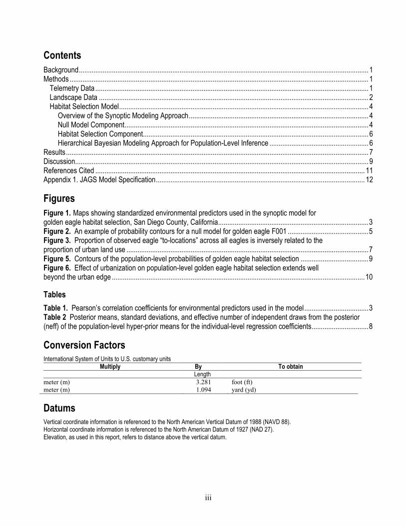
Contents Background .............................................................................................................................................................. 1 Methods ................................................................................................................................................................... 1

Telemetry Data ..................................................................................................................................................... 1 Landscape Data ................................................................................................................................................... 2 Habitat Selection Model ........................................................................................................................................ 4

Overview of the Synoptic Modeling Approach .................................................................................................. 4 Null Model Component ..................................................................................................................................... 4 Habitat Selection Component ........................................................................................................................... 6 Hierarchical Bayesian Modeling Approach for Population-Level Inference ...................................................... 6

Results ..................................................................................................................................................................... 7 Discussion................................................................................................................................................................ 9 References Cited ................................................................................................................................................... 11 Appendix 1. JAGS Model Specification .................................................................................................................. 12

Figures Figure 1. Maps showing standardized environmental predictors used in the synoptic model for golden eagle habitat selection, San Diego County, California .................................................................................. 3 Figure 2. An example of probability contours for a null model for golden eagle F001 ............................................ 5 Figure 3. Proportion of observed eagle “to-locations” across all eagles is inversely related to the proportion of urban land use .................................................................................................................................... 7 Figure 5. Contours of the population-level probabilities of golden eagle habitat selection ..................................... 9 Figure 6. Effect of urbanization on population-level golden eagle habitat selection extends well beyond the urban edge .......................................................................................................................................... 10

Tables Table 1. Pearson’s correlation coefficients for environmental predictors used in the model ................................... 3 Table 2 Posterior means, standard deviations, and effective number of independent draws from the posterior (neff) of the population-level hyper-prior means for the individual-level regression coefficients ............................... 8

Conversion Factors International System of Units to U.S. customary units

Multiply By To obtain Length

meter (m) 3.281 foot (ft) meter (m) 1.094 yard (yd)

Datums Vertical coordinate information is referenced to the North American Vertical Datum of 1988 (NAVD 88). Horizontal coordinate information is referenced to the North American Datum of 1927 (NAD 27). Elevation, as used in this report, refers to distance above the vertical datum.

iv

This page left intentionally blank

1

Golden Eagle (Aquila chrysaetos) Habitat Selection as a Function of Land Use and Terrain, San Diego County, California

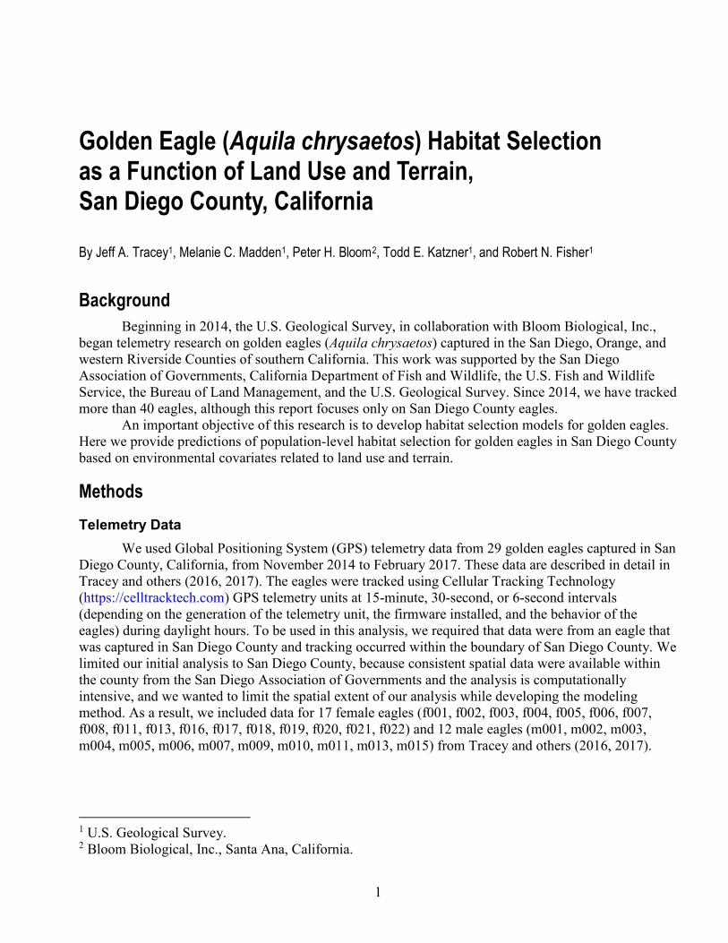
By Jeff A. Tracey1, Melanie C. Madden1, Peter H. Bloom2, Todd E. Katzner1, and Robert N. Fisher1

Background Beginning in 2014, the U.S. Geological Survey, in collaboration with Bloom Biological, Inc.,

began telemetry research on golden eagles (Aquila chrysaetos) captured in the San Diego, Orange, and western Riverside Counties of southern California. This work was supported by the San Diego Association of Governments, California Department of Fish and Wildlife, the U.S. Fish and Wildlife Service, the Bureau of Land Management, and the U.S. Geological Survey. Since 2014, we have tracked more than 40 eagles, although this report focuses only on San Diego County eagles.

An important objective of this research is to develop habitat selection models for golden eagles. Here we provide predictions of population-level habitat selection for golden eagles in San Diego County based on environmental covariates related to land use and terrain.

Methods Telemetry Data

We used Global Positioning System (GPS) telemetry data from 29 golden eagles captured in San Diego County, California, from November 2014 to February 2017. These data are described in detail in Tracey and others (2016, 2017). The eagles were tracked using Cellular Tracking Technology (https://celltracktech.com) GPS telemetry units at 15-minute, 30-second, or 6-second intervals (depending on the generation of the telemetry unit, the firmware installed, and the behavior of the eagles) during daylight hours. To be used in this analysis, we required that data were from an eagle that was captured in San Diego County and tracking occurred within the boundary of San Diego County. We limited our initial analysis to San Diego County, because consistent spatial data were available within the county from the San Diego Association of Governments and the analysis is computationally intensive, and we wanted to limit the spatial extent of our analysis while developing the modeling method. As a result, we included data for 17 female eagles (f001, f002, f003, f004, f005, f006, f007, f008, f011, f013, f016, f017, f018, f019, f020, f021, f022) and 12 male eagles (m001, m002, m003, m004, m005, m006, m007, m009, m010, m011, m013, m015) from Tracey and others (2016, 2017).

1 U.S. Geological Survey. 2 Bloom Biological, Inc., Santa Ana, California.

2

Landscape Data In this model, we used four environmental predictors: (1) the proportion of urban development

within a 1,000-m radius circular moving window, (2) the proportion of exurban development within a 1,000-m radius circular moving window, (3) vector ruggedness measure (VRM; Sappington and others, 2007) calculated within a 500-m radius circular moving window, and (4) topographic position index (TPI; De Reu and others, 2013) calculated within a 500-m radius circular moving window (fig. 1). The radii used to calculate environmental predictors were postulated to be representative of the scale at which eagles interacted with these features. Layers for the proportion of urban and exurban development were derived from reclassified and rasterized 2014 land use data produced and maintained by the San Diego Association of Governments (SanDAG; SanGIS, 2015). Terrain metrics were calculated using 10-m USGS digital elevations that were rescaled to 100-m resolution. VRM describes heterogeneity of the slope and aspect of the terrain within the moving window, and hence, is a measure of ruggedness. TPI quantifies the elevation of a point in relation to the average elevation within the moving window centered on the point; if the point is higher than its average surroundings, TPI is positive and if it is lower, TPI is negative. All predictors were stored in rasters with 100×100-m cells covering the same extent. All four predictors had low Pearson’s correlation coefficients (table 1) and were standardized (to have a mean of 0 and standard deviation of 1) prior to use in modeling which allows us to directly compare regression coefficients to evaluate the relative influence of each predictor.

3

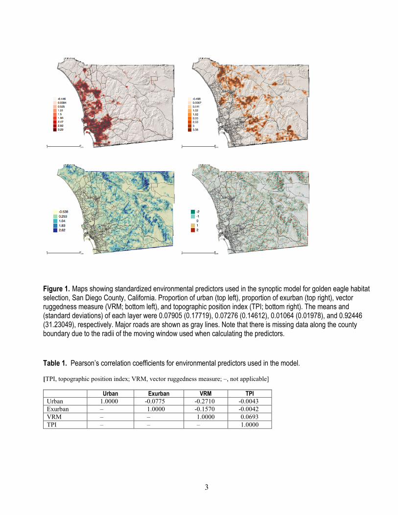
Figure 1. Maps showing standardized environmental predictors used in the synoptic model for golden eagle habitat selection, San Diego County, California. Proportion of urban (top left), proportion of exurban (top right), vector ruggedness measure (VRM; bottom left), and topographic position index (TPI; bottom right). The means and (standard deviations) of each layer were 0.07905 (0.17719), 0.07276 (0.14612), 0.01064 (0.01978), and 0.92446 (31.23049), respectively. Major roads are shown as gray lines. Note that there is missing data along the county boundary due to the radii of the moving window used when calculating the predictors.

Table 1. Pearson’s correlation coefficients for environmental predictors used in the model.

[TPI, topographic position index; VRM, vector ruggedness measure; –, not applicable]

Urban Exurban VRM TPI Urban 1.0000 -0.0775 -0.2710 -0.0043Exurban – 1.0000 -0.1570 -0.0042VRM – – 1.0000 0.0693 TPI – – – 1.0000

4

Habitat Selection Model

Overview of the Synoptic Modeling Approach We modeled habitat selection using a hierarchical Bayesian implementation of the synoptic

modeling approach, which provides a natural way to incorporate non-uniform availability of spatial locations at the individual level (Thomas and others, 2006; Horne and others, 2008; Tinker and others, 2017). The synoptic model consists of a null model for an individual’s space-use and a regression component that weights the null model as a function of environmental predictors. Conceptually, the null models reflect what is available to individual eagles given their tendency to remain in a general area (Horne and others, 2008). The null model for each individual is further weighted by a function of environmental predictors. This weighting describes habitat selection. The estimated population-level parameters of this function are then used to predict habitat selection across the entire area.

Null Model Component For each eagle, we developed kernel-based null models for the probability of space-use in the

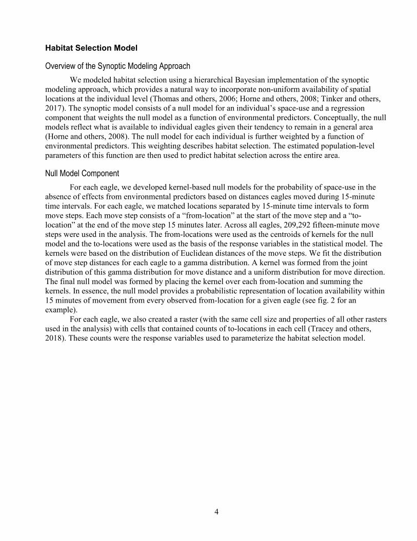
absence of effects from environmental predictors based on distances eagles moved during 15-minute time intervals. For each eagle, we matched locations separated by 15-minute time intervals to form move steps. Each move step consists of a “from-location” at the start of the move step and a “to-location” at the end of the move step 15 minutes later. Across all eagles, 209,292 fifteen-minute move steps were used in the analysis. The from-locations were used as the centroids of kernels for the null model and the to-locations were used as the basis of the response variables in the statistical model. The kernels were based on the distribution of Euclidean distances of the move steps. We fit the distribution of move step distances for each eagle to a gamma distribution. A kernel was formed from the joint distribution of this gamma distribution for move distance and a uniform distribution for move direction. The final null model was formed by placing the kernel over each from-location and summing the kernels. In essence, the null model provides a probabilistic representation of location availability within 15 minutes of movement from every observed from-location for a given eagle (see fig. 2 for an example).

For each eagle, we also created a raster (with the same cell size and properties of all other rasters used in the analysis) with cells that contained counts of to-locations in each cell (Tracey and others, 2018). These counts were the response variables used to parameterize the habitat selection model.

5

Figure 2. An example of probability contours for a null model for golden eagle F001. The eagle “from-locations” on which the null model is based are shown as white points with black fill. The contours are 100 percent (dark gray), 99 percent (teal), 95 percent (dark teal), 90 percent (lightest orange), 80, 70, 60, and 50 percent (darkest orange).

6

Habitat Selection Component Following the synoptic modeling approach for habitat suitability, we weight the null model

within each grid cell by an exponential function of the four environmental predictors in that cell (Thomas and others, 2006; Johnson and others, 2008). This represents the selection of grid cells by the individual at a level above or below that specified by the null model.

More formally, the general form of the synoptic model at the individual level is:

𝑝𝑝𝑖𝑖�𝒔𝒔�𝒙𝒙𝑠𝑠, β𝒊𝒊� = 𝑎𝑎𝑖𝑖𝑠𝑠 × exp(∑ 𝑥𝑥𝑠𝑠,𝑗𝑗

4𝑗𝑗=1 × 𝛽𝛽𝑖𝑖,𝑗𝑗)

∑ 𝑎𝑎𝑖𝑖𝑠𝑠 × exp(∑ 𝑥𝑥𝑠𝑠,𝑗𝑗4𝑗𝑗=1 × 𝛽𝛽𝑖𝑖,𝑗𝑗)𝑠𝑠

where ais is the probability density from the null model for individual eagle i in raster cell s, xs = (xs,1, …, xs,4)′ is a vector of environmental predictors (in order of urban, exurban, VRM, and TPI) for raster cell s, and βi = (βi,1, …, βi,4)′ is a vector of regression coefficients for individual i that must be estimated. The function exp(∑ 𝑥𝑥𝑠𝑠,𝑗𝑗

4𝑗𝑗=1 × 𝛽𝛽𝑖𝑖,𝑗𝑗) modifies the null distribution. In the denominator, the

function is summed over all raster cells to yield a normalizing constant. This individual-level spatial probability distribution represents the probability that a given eagle

will select each raster cell in the study area. Thus, when we multiply this probability density by the total number of to-locations for that individual, we get an expected count of that eagle’s locations within each raster cell. Following Tinker and others (2017), we assume a Poisson distribution for the counts; hence, the final statistical model at the individual level is:

𝑝𝑝�𝑐𝑐𝑖𝑖,𝑠𝑠�𝒙𝒙𝑠𝑠, β𝒊𝒊�~𝑃𝑃𝑃𝑃𝑃𝑃𝑃𝑃𝑃𝑃𝑃𝑃𝑃𝑃(𝑁𝑁𝑖𝑖 × 𝑝𝑝𝑖𝑖�𝒔𝒔�𝒙𝒙𝑠𝑠, β𝒊𝒊�)

Where cis is the count of the telemetry locations for the ith eagle in raster cell s and Ni is the total number of to-locations for eagle i, as described at the end of the section on null models.

Hierarchical Bayesian Modeling Approach for Population-Level Inference Raster cells were the unit of analysis. Each cell contained a vector of values for each of the four

environmental predictors and a vector of response variables which were the to-location counts for each of the 29 eagles in the cell. Hence, our response variable was multivariate. Due to the number of cells (i.e. 1,049,102 data-containing cells) in the spatial raster storing the data, we randomly sampled 100,000 cells without replacement to form the final dataset used for the Bayesian analysis.

We took a hierarchical Bayesian modeling approach to allow estimation of the regression parameters for each individual eagle (the βi values) that are drawn from population-level distributions, each distribution with population-level mean and standard deviation hyper-parameters. The individual-level regression coefficients depend on population-level hyper-priors ϕj and σj by 𝛽𝛽𝑖𝑖,𝑗𝑗~𝑁𝑁𝑃𝑃𝑁𝑁𝑁𝑁𝑎𝑎𝑁𝑁(𝜑𝜑𝑗𝑗, 1/𝜎𝜎𝑗𝑗). The population-level priors are uninformative priors 𝜑𝜑𝑗𝑗~𝑁𝑁𝑃𝑃𝑁𝑁𝑁𝑁𝑎𝑎𝑁𝑁(0, 1/1000) and 𝜎𝜎𝑗𝑗~𝑈𝑈𝑃𝑃𝑃𝑃𝑈𝑈𝑃𝑃𝑁𝑁𝑁𝑁(0, 100). This provided simultaneous individual-level and population-level inference of habitat selection parameters. Samples from the posterior distribution of 124 (8 population-level hyper-parameters and 4 individual-level parameters for each of the 29 eagles) were simulated using JAGS (Just Another Gibbs Sampler; Plummer, 2015) from R (R Core Team, 2017) via the runjags package (Denwood, 2016).

The final population-level predictions of habitat selection are based on a null model of uniform availability weighted by the function of environmental covariates using the population-level parameter estimates (Tinker and others, 2017).

7

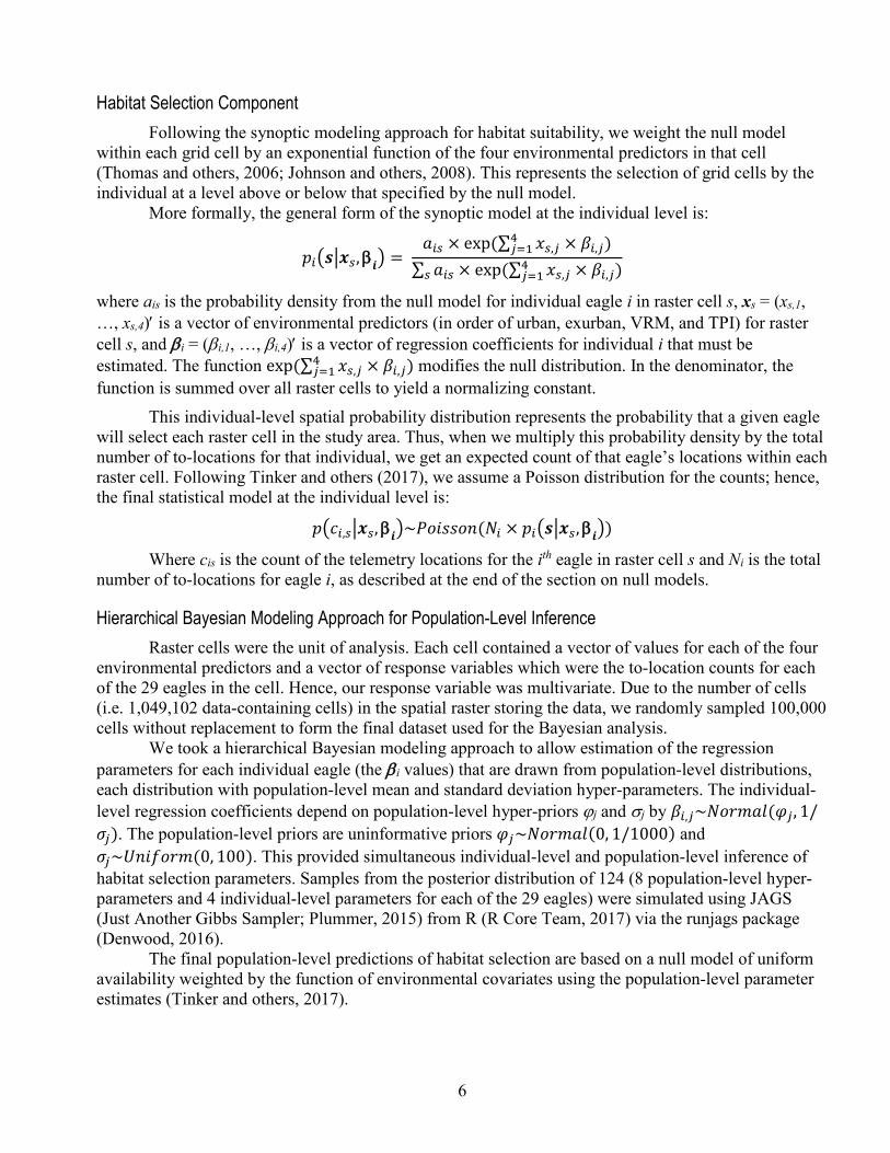
Results An exploration of the data shows that the count of all eagle to-locations divided by the total

number of to-locations increases as the proportion of urban land use within 1,000 m within cells decreases (fig. 3).

Figure 3. Proportion of observed eagle “to-locations” across all eagles is inversely related to the proportion of urban land use. On the y-axis is 1 + the count of all eagle locations in the cell divided by 1 + the count of eagle locations across all cells (on a log scale). One was added so the natural logarithm of the normalized count would be finite if the count was zero. The proportion of urban land use within 1,000-meter radius circular window around the cell is shown on the x-axis.

Four independent chains of 5,000 samples (after discarding 1,000 burn-in samples) from the

joint posterior distribution of 155 unknown model parameters were generated using JAGS. All 155 model parameters (10 population-level parameters (mean and standard deviation hyper-priors) and 5 individual-level parameters for 29 eagles) successfully converged based on diagnostic output (effective samples sizes were greater than 1,700, R-hat values were ≈ 1, and autocorrelation was small for all individual-level and population-level parameters). Population-level parameter posterior means are given in table 2. The population-level parameter values indicate strong avoidance of urban development including areas near urban development, moderate avoidance of exurban development, weak selection in favor of rugged terrain (as quantified by VRM), and moderate selection in favor of areas higher than those surrounding it (as quantified by TPI).

8

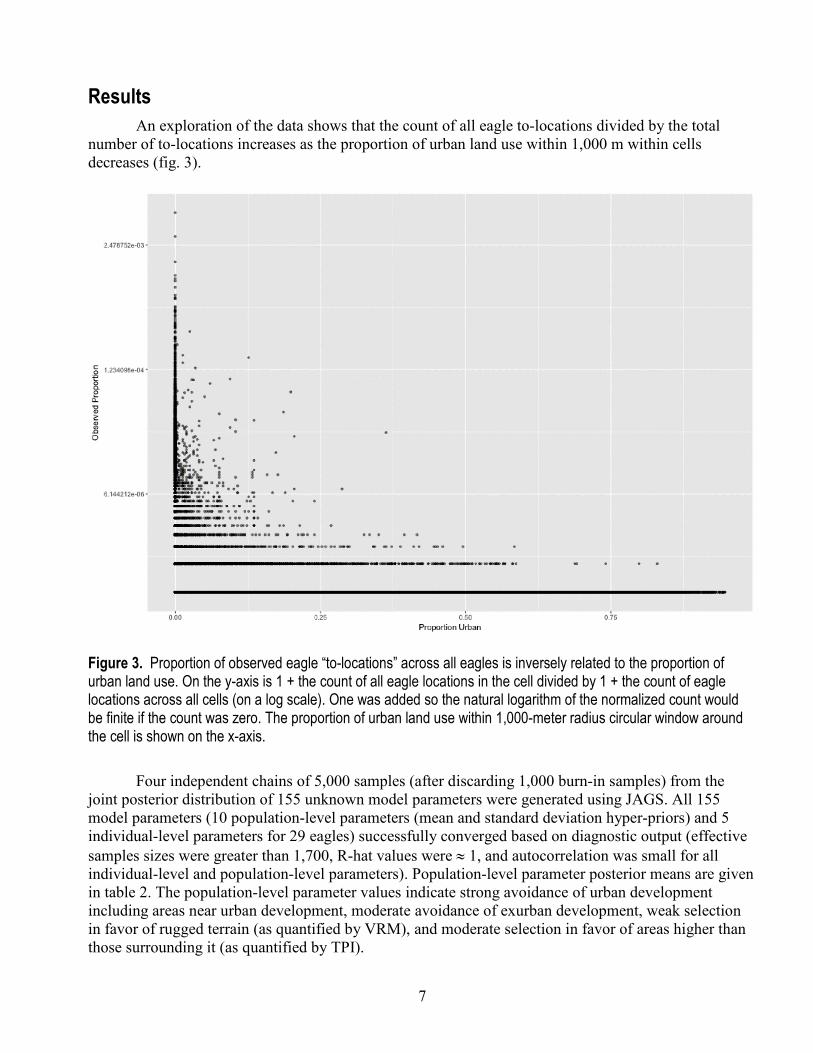
Table 1 Posterior means, standard deviations, and effective number of independent draws from the posterior (neff) of the population-level hyper-prior means for the individual-level regression coefficients.

Parameter Predictor Mean SD neff ϕ1 Proportion urban -2.879988 0.704036 3,260 ϕ2 Proportion exurban -0.790471 0.181360 8,216 ϕ3 VRM 0.130581 0.116530 12,922 ϕ4 TPI 0.681908 0.100178 15,580

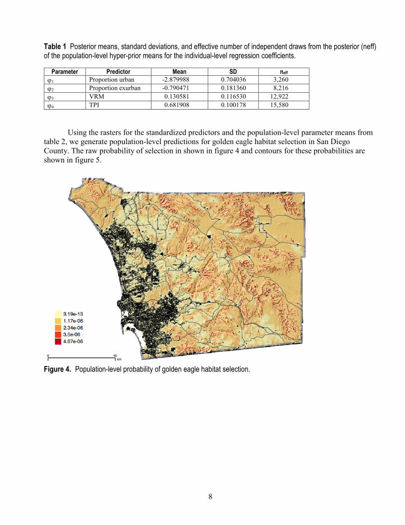
Using the rasters for the standardized predictors and the population-level parameter means from

table 2, we generate population-level predictions for golden eagle habitat selection in San Diego County. The raw probability of selection in shown in figure 4 and contours for these probabilities are shown in figure 5.

Figure 4. Population-level probability of golden eagle habitat selection.

9

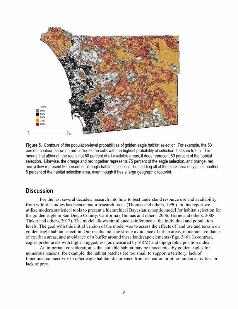
Figure 5. Contours of the population-level probabilities of golden eagle habitat selection. For example, the 50 percent contour, shown in red, includes the cells with the highest probability of selection that sum to 0.5. This means that although the red is not 50 percent of all available areas, it does represent 50 percent of the habitat selection. Likewise, the orange and red together represents 75 percent of the eagle selection, and orange, red, and yellow represent 90 percent of all eagle habitat selection. Thus adding all of the black area only gains another 5 percent of the habitat selection area, even though it has a large geographic footprint.

Discussion For the last several decades, research into how to best understand resource use and availability

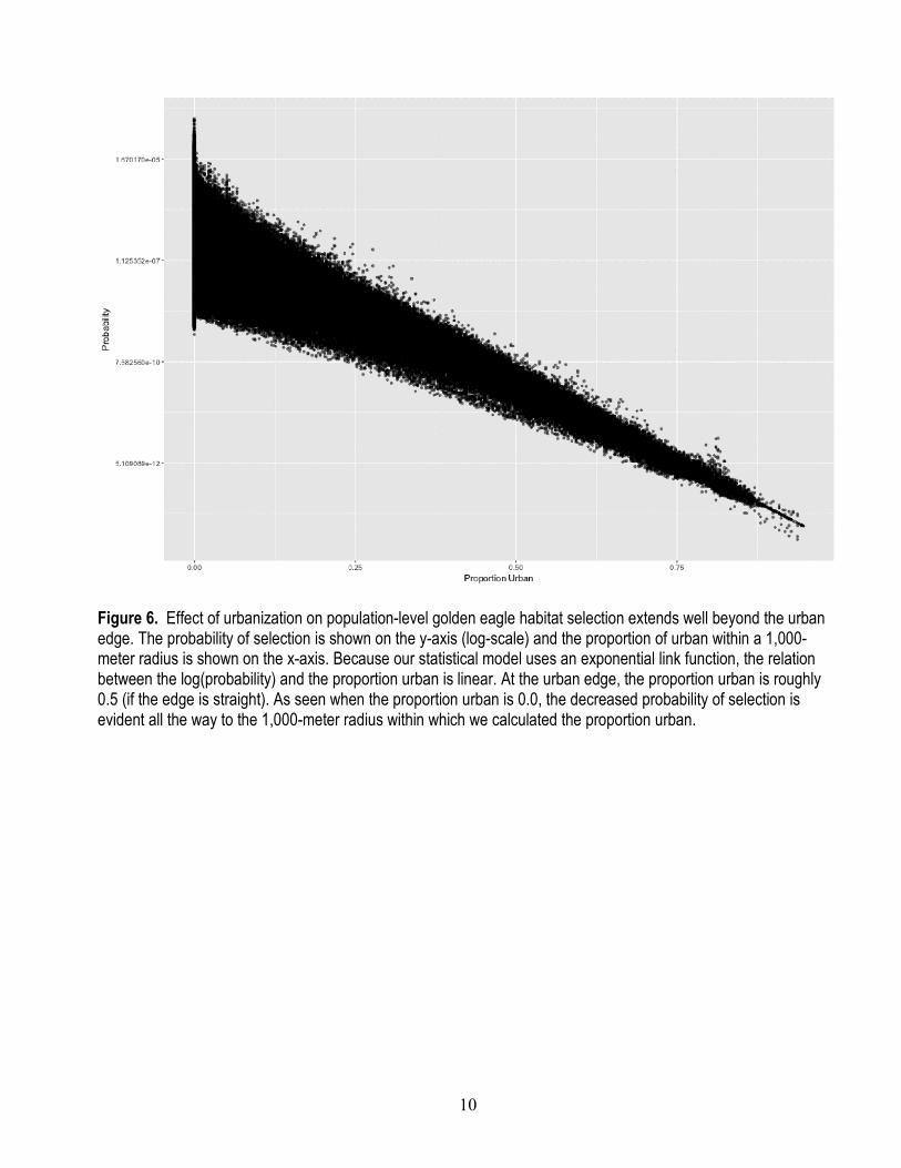
from wildlife studies has been a major research focus (Thomas and others, 1990). In this report we utilize modern statistical tools to present a hierarchical Bayesian synoptic model for habitat selection for the golden eagle in San Diego County, California (Thomas and others, 2006; Horne and others, 2008; Tinker and others, 2017). The model allows simultaneous inference at the individual and population levels. The goal with this initial version of the model was to assess the effects of land use and terrain on golden eagle habitat selection. Our results indicate strong avoidance of urban areas, moderate avoidance of exurban areas, and avoidance of a buffer around these landscape elements (figs. 3–6). In contrast, eagles prefer areas with higher ruggedness (as measured by VRM) and topographic position index.

An important consideration is that suitable habitat may be unoccupied by golden eagles for numerous reasons; for example, the habitat patches are too small to support a territory, lack of functional connectivity to other eagle habitat, disturbance from recreation or other human activities, or lack of prey.

10

Figure 6. Effect of urbanization on population-level golden eagle habitat selection extends well beyond the urban edge. The probability of selection is shown on the y-axis (log-scale) and the proportion of urban within a 1,000-meter radius is shown on the x-axis. Because our statistical model uses an exponential link function, the relation between the log(probability) and the proportion urban is linear. At the urban edge, the proportion urban is roughly 0.5 (if the edge is straight). As seen when the proportion urban is 0.0, the decreased probability of selection is evident all the way to the 1,000-meter radius within which we calculated the proportion urban.

11

References Cited De Reu, J., Bourgeois, J., Bats, M., Zwertvaegher, A., Gelorini, V., De Smedt, P., Chu, W., Antrop, M.,

De Maeyer, P., Finke, P., and Van Meirvenne, M., 2013, Application of the topographic position index to heterogeneous landscapes: Geomorphology, v. 186, p. 39–49.

Denwood, M.J., 2016, runjags: An {R} package providing interface utilities, odel templates, parallel computing methods and additional distributions for {MCMC} models in JAGS: Journal of Statistical Software, v. 71, no. 9, p. 1–25, doi 10.18637/jss.v071.i09.

Horne, J.S., Garton, E.O., and Rachlow, J.L., 2008, A synoptic model of animal space use—Simultaneous estimation of home range, habitat selection, and inter/intra-specific relationships: Ecological Modelling, v. 214, nos. 2–4, p. 338–348.

Johnson, C.J., and Gillingham, M.P., 2008, Sensitivity of species-distribution models to error, bias, and model design: An application to resource selection functions for woodland caribou: Ecological modelling, v. 213, no. 2, 143-155.

Plummer, M., 2015, JAGS Version 4.0. 0 user manual: JAGS, Just Another Gibbs Sampler, open-source software, user manual, accessed April 10, 2018, at https://sourceforge.net/projects/mcmc-jags/files/Manuals/4.x.

R Core Team, 2017, R—A language and environment for statistical computing: Vienna, Austria, R Foundation for Statistical Computing, accessed April 10, 2018, at https://www.R-project.org/.

SanGIS, 2015, LAND_USE_2015, at http://rdw.sandag.org/Account/gisdtview?dir=Land%20Use. Sappington, J.M., Longshore, K.M., and Thompson, D.B., 2007, Quantifying landscape ruggedness for

animal habitat analysis—A case study using bighorn sheep in the Mojave Desert: Journal of wildlife management, v. 71, no. 5, 1419–1426.

Thomas, D.L., Johnson, D., and Griffith, B., 2006, A Bayesian random effects discrete-choice model for resource selection: population-level selection inference: Journal of Wildlife Management, v. 70, no. 2, p. 404-412.

Thomas, D.L., and Taylor, E.J., 1990, Study designs and tests for comparing resource use and availability: Journal of Wildlife Management, v. 54, no. 2, p. 322-330.

Tinker, M.T., Tomoleoni, J., LaRoche, N., Bowen, L., Miles, A.K., Murray, M., Staedler, M., and Randell, Z., 2017, Southern sea otter range expansion and habitat use in the Santa Barbara Channel, California: U.S. Geological Survey Open-File Report 2017–1001 (OCS Study BOEM 2017-002), 76 p., https://doi.org/10.3133/ofr20171001.

Tracey, J.A., Madden, M.C., Bloom, P.H., Katzner, T.E., and Fisher, R.N., 2018, Predictor, null model, response variable, and habitat suitability prediction rasters for a golden eagle hierarchical Bayesian synoptic model used for habitat selection in San Diego County, California, derived from golden eagle data collected from November 2014–February 2017: U.S. Geological Survey data release, https://doi.org/10.5066/P9OZVGEG.

Tracey, J.A., Madden, M.C., Sebes, J.B., Bloom, P.H., Katzner, T.E., and Fisher, R.N., 2016, Biotelemetry data for golden eagles (Aquila chrysaetos) captured in coastal southern California, November 2014–February 2016: U.S. Geological Survey Data Series 994, 32 p., http://dx.doi.org/10.3133/ds994.

Tracey, J.A., Madden, M.C., Sebes, J.B., Bloom, P.H., Katzner, T.E., and Fisher, R.N., 2017, Bioltelemetery data for golden eagles (Aquila chrysaetos) captured in coastal southern California, February 2016–February 2017: U.S. Geological Survey Data Series 1051, 35 p., https://doi.org/10.3133/ds1051.

12

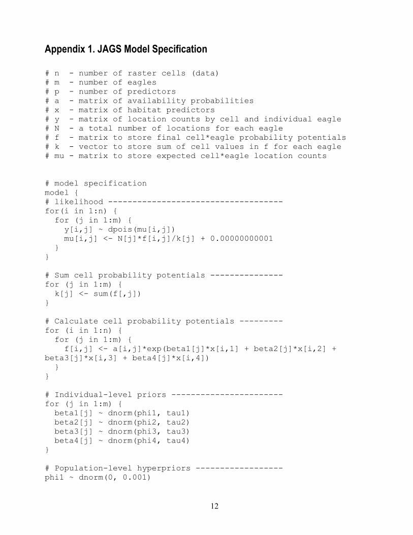
Appendix 1. JAGS Model Specification # n - number of raster cells (data) # m - number of eagles # p - number of predictors # a - matrix of availability probabilities # x - matrix of habitat predictors # y - matrix of location counts by cell and individual eagle # N - a total number of locations for each eagle # f - matrix to store final cell*eagle probability potentials # k - vector to store sum of cell values in f for each eagle # mu - matrix to store expected cell*eagle location counts # model specification model { # likelihood ------------------------------------ for(i in 1:n) { for (j in 1:m) { y[i,j] ~ dpois(mu[i,j]) mu[i,j] <- N[j]*f[i,j]/k[j] + 0.00000000001 } } # Sum cell probability potentials --------------- for (j in 1:m) { k[j] <- sum(f[,j]) } # Calculate cell probability potentials --------- for (i in 1:n) { for (j in 1:m) { f[i,j] <- a[i,j]*exp(beta1[j]*x[i,1] + beta2[j]*x[i,2] + beta3[j]*x[i,3] + beta4[j]*x[i,4]) } } # Individual-level priors ----------------------- for (j in 1:m) { beta1[j] ~ dnorm(phi1, tau1) beta2[j] ~ dnorm(phi2, tau2) beta3[j] ~ dnorm(phi3, tau3) beta4[j] ~ dnorm(phi4, tau4) } # Population-level hyperpriors ------------------ phi1 ~ dnorm(0, 0.001)

13

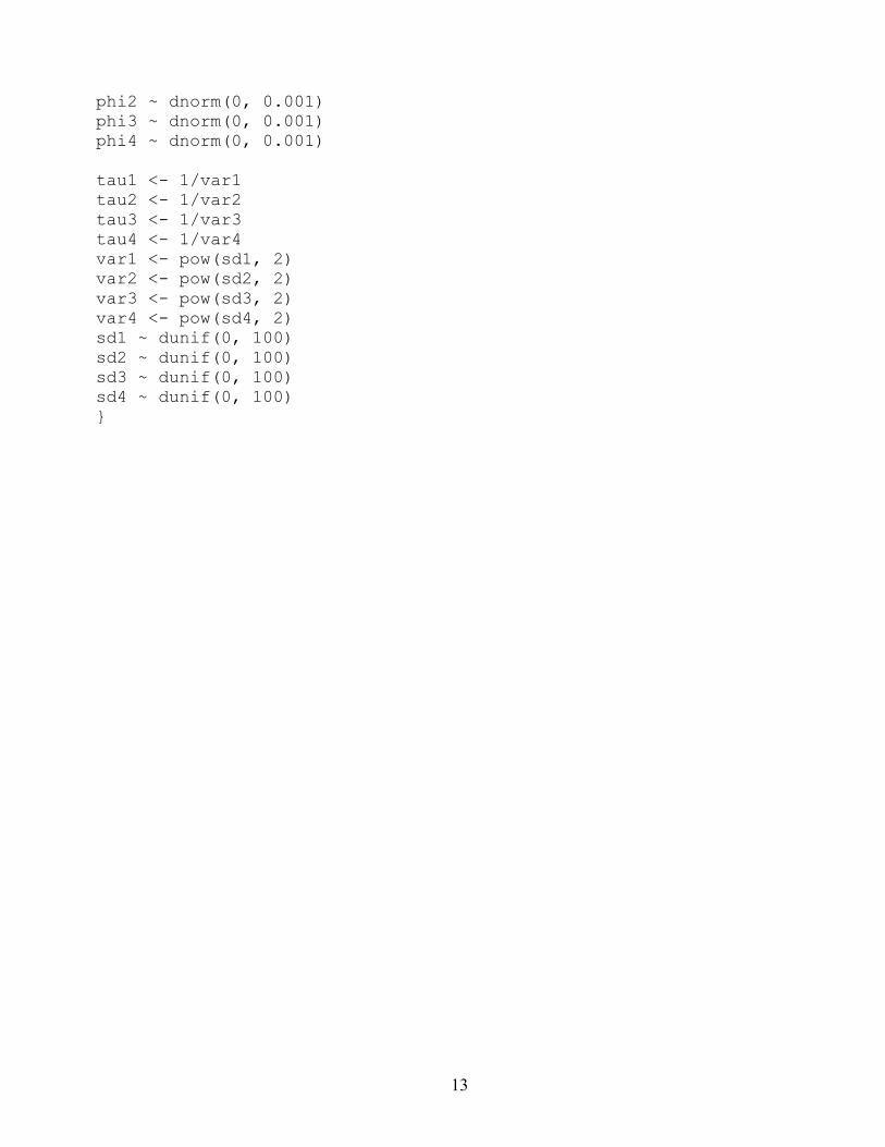
phi2 ~ dnorm(0, 0.001) phi3 ~ dnorm(0, 0.001) phi4 ~ dnorm(0, 0.001) tau1 <- 1/var1 tau2 <- 1/var2 tau3 <- 1/var3 tau4 <- 1/var4 var1 <- pow(sd1, 2) var2 <- pow(sd2, 2) var3 <- pow(sd3, 2) var4 <- pow(sd4, 2) sd1 ~ dunif(0, 100) sd2 ~ dunif(0, 100) sd3 ~ dunif(0, 100) sd4 ~ dunif(0, 100) }

Publishing support provided by the U.S. Geological SurveyScience Publishing Network, Tacoma Publishing Service Center

For more information concerning the research in this report, contact the Director, Western Ecological Research CenterU.S. Geological Survey3020 State University Drive EastSacramento, California 95819https://www.werc.usgs.gov/

Tracey and others—Golden Eagle (Aquila chrysaetos) Habitat Selection as a Function of Land Use and Terrain, San Diego County, California—

Open-File Report 2018-1067ISSN 2331-1258 (online)https://doi.org/10.3133/ofr20181067