GOING FROM 12-KM TO 250-M RESOLUTION

Josephine Bates1, Audrey Flak2, Howard Chang2, Heather Holmes3, David Lavoue1, Mitchel Klein2, Matthew Strickland2, Lyndsey Darrow2, James

Mulholland1, Armistead Russell11Georgia Institute of Technology 2 Emory University 3 University of Nevada, Reno

Comparison of Two Downscaling Techniques

R834799

SCAPE

2

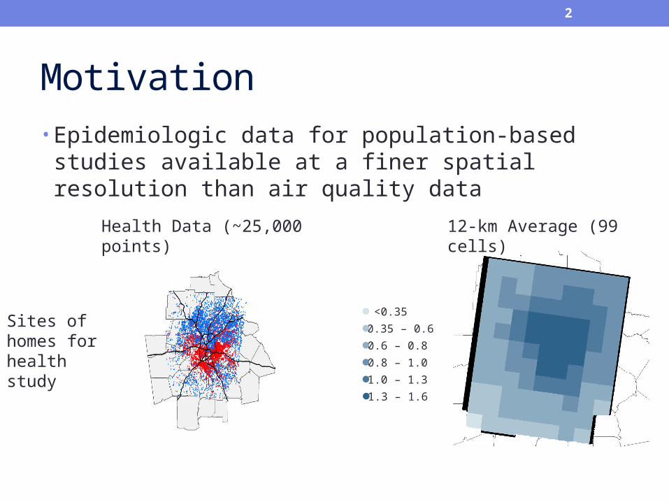
Motivation• Epidemiologic data for population-based studies available

at a finer spatial resolution than air quality data

0.6 – 0.8

0.8 – 1.0

1.0 – 1.3

0.35 – 0.6

<0.35

1.3 – 1.6

12-km Average (99 cells)Health Data (~25,000 points)

Sites of homes for health study

3

Goal• Goal: Develop a method for estimating daily exposure

estimates at 250-m grid resolution using 12-km CMAQ data for a birth cohort study

• Two approaches:

1. Bayesian Statistical Downscaler

2. CTM - Dispersion Model Fusion

4

APPROACH 1Bayesian Statistical Downscaler

5

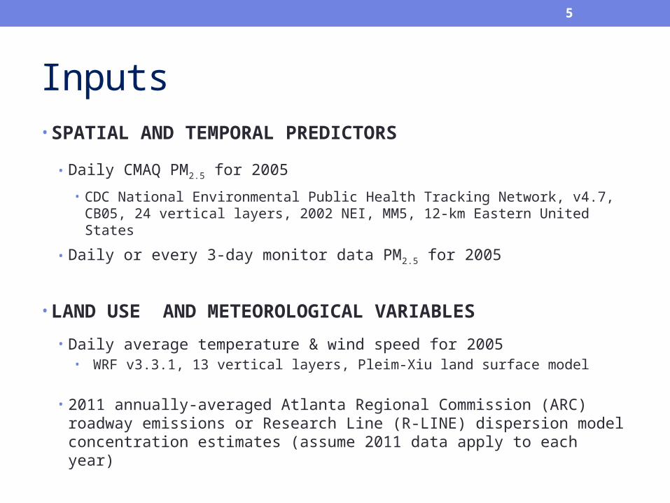
Inputs• SPATIAL AND TEMPORAL PREDICTORS

• Daily CMAQ PM2.5 for 2005

• CDC National Environmental Public Health Tracking Network, v4.7, CB05, 24 vertical layers, 2002 NEI, MM5, 12-km Eastern United States

• Daily or every 3-day monitor data PM2.5 for 2005

• LAND USE AND METEOROLOGICAL VARIABLES

• Daily average temperature & wind speed for 2005• WRF v3.3.1, 13 vertical layers, Pleim-Xiu land surface model

• 2011 annually-averaged Atlanta Regional Commission (ARC) roadway emissions or Research Line (R-LINE) dispersion model concentration estimates (assume 2011 data apply to each year)

6

Inputs

2011 ARC Emissions

Link-based emissions

in g/day/m provided by the

Atlanta Regional Commission

7

Inputs

R-LINE is a line-source dispersion model for near-surface releases developed by the EPA

ΔPM2.5 = 10 [0.32*log(RLINE_PM2.5) - 0.05)

We adjusted the R-LINE estimates using a three-step process

1. Fit R-LINE estimates to Chemical Mass Balance (CMB) vehicle source estimates

2. Fit R-LINE estimates to monitor values (after subtracting out background PM2.5)

3. Average the coefficients from each fitXinxin Zhai, et al. “Comparison and calibration of Research-Line (RLINE) model results with measurement-based and CMAQ-based source impacts” , 14th Annual CMAS Conference. Chapel Hill, NC. 2015

8

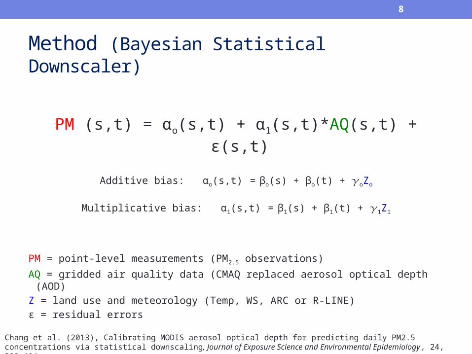
Method (Bayesian Statistical Downscaler)

PM (s,t) = αo(s,t) + α1(s,t)*AQ(s,t) + ε(s,t)

Additive bias: αo(s,t) = βo(s) + βo(t) + 𝛾oZo

Multiplicative bias: α1(s,t) = β1(s) + β1(t) + 𝛾1Z1

PM = point-level measurements (PM2.5 observations)

AQ = gridded air quality data (CMAQ replaced aerosol optical depth (AOD)

Z = land use and meteorology (Temp, WS, ARC or R-LINE)

ε = residual errorsChang et al. (2013), Calibrating MODIS aerosol optical depth for predicting daily PM2.5 concentrations via statistical downscaling , Journal of Exposure Science and Environmental Epidemiology, 24, 398-404.

9

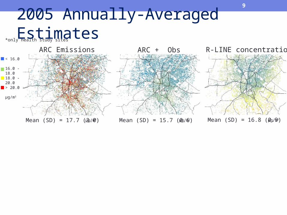
ARC Emissions R-LINE concentrationsARC + Obs

2005 Annually-Averaged Estimates*only health study sites

Mean (SD) = 16.8 (0.9) Mean (SD) = 17.7 (3.0) Mean (SD) = 15.7 (0.6)

μg/m3

μg/m3 μg/m3 μg/m3

18.0 - 20.0

< 16.0

16.0 - 18.0

> 20.0

10

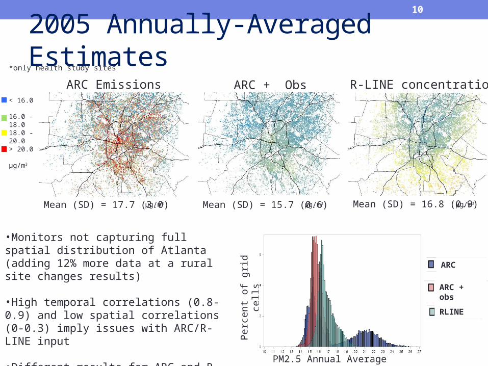
ARC Emissions R-LINE concentrationsARC + Obs

2005 Annually-Averaged Estimates*only health study sites

Mean (SD) = 16.8 (0.9) Mean (SD) = 17.7 (3.0) Mean (SD) = 15.7 (0.6)

Per

cen

t of

grid

cel

ls

RLINE

ARC

ARC + obs

μg/m3 μg/m3 μg/m3

PM2.5 Annual Average Estimates

•Monitors not capturing full spatial distribution of Atlanta (adding 12% more data at a rural site changes results)

•High temporal correlations (0.8-0.9) and low spatial correlations (0-0.3) imply issues with ARC/R-LINE input

•Different results for ARC and R-LINE inputs

μg/m3

18.0 - 20.0

< 16.0

16.0 - 18.0

> 20.0

11

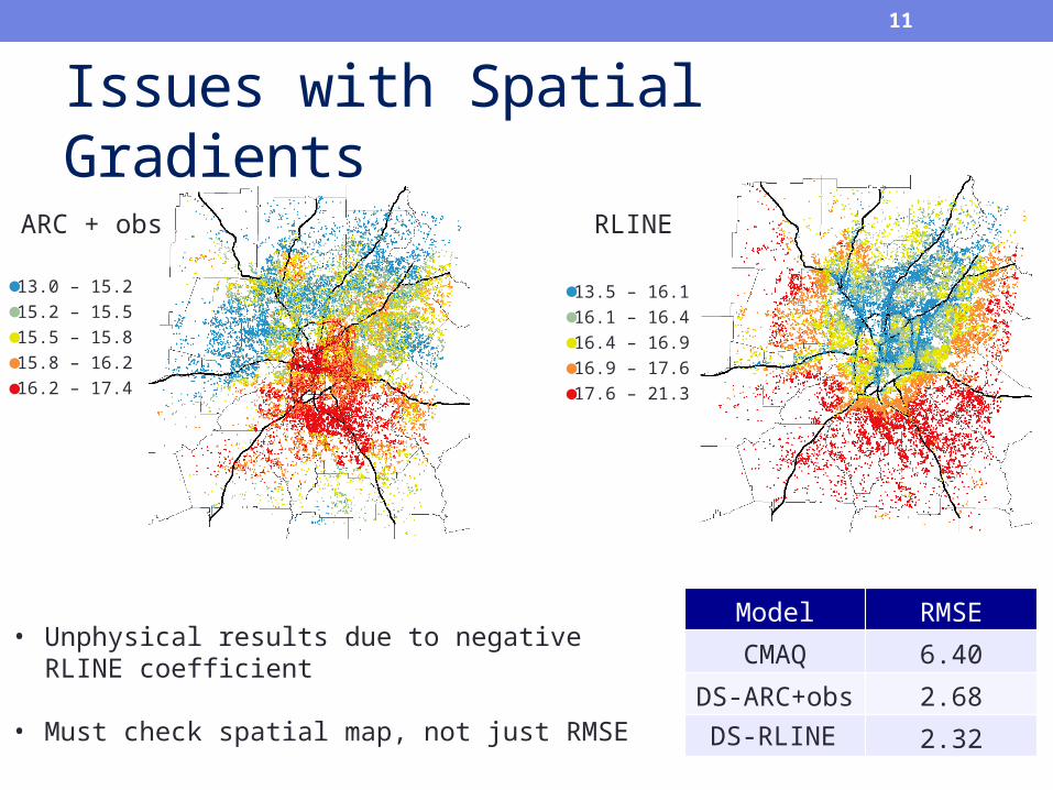
Issues with Spatial Gradients

13.5 – 16.1

16.1 – 16.4

16.4 – 16.9

16.9 – 17.6

17.6 – 21.3

13.0 – 15.2

15.2 – 15.5

15.5 – 15.8

15.8 – 16.2

16.2 – 17.4

ARC + obs RLINE

Model RMSE

CMAQ 6.40

DS-ARC+obs 2.68

2.32

• Unphysical results due to negative RLINE coefficient

• Must check spatial map, not just RMSEDS-RLINE

12

Conclusions (Bayesian Statistical Downscaler)

• Results very dependent on number of monitor values it is trained on (CO, NO2)

• Results very dependent on land-use variables (ARC vs. R-LINE)

• Downscaler not yet ready to be used with CMAQ and

R-LINE

13

APPROACH 2CTM – Dispersion Model Fusion

14

Inputs• Dispersion Model

• 2011 RLINE estimations adjusted using observations• Assume 2011 RLINE estimations apply to each year• 250-m resolution

• Chemical Transport Model• CMAQ-OBS : must adjust CMAQ values using observations before

inputting into CTM-Dispersion model• 12-km resolution

Scale 12-km CMAQ using fine-scale dispersion model

vehicle source impact estimates from R-LINE

15

25

0

1

0

21* )1( RFRFR 21

* )1( CFCFC

Fused Field andTemporal Correlation Estimation

C*

CMAQ

Observations

PM2.5 (g/m3), 7/23/08

Data-Fused CMAQ-OBS

optimized for temporal variation

temporal variation from OBS;spatial structure from mean CMAQ

temporal variation & spatial structure from CMAQ; scaled to mean OBS

Zhai, et al. “Spatiotemporal error assessment for ambient air pollution estimates obtained using an observation-CMAQ data fusion technique”, 13th annual CMAS Conference

16

Method (CTM-Dispersion Model Fusion)

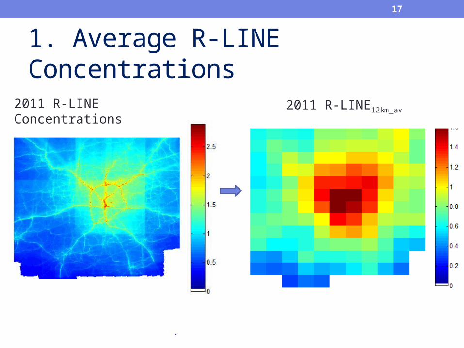
1. Spatially average R-LINE values to grid scale of CMAQ-OBS (12-km)

2. Subtract averaged R-LINE concentrations from CMAQ-OBS values to remove mobile impacts on PM2.5

3. Spatially interpolate this result using bilinear interpolation to obtain spatially smooth estimates at the grid scale of R-LINE concentrations (250-m)

4. Add R-LINE estimated PM2.5 to results of step 3 to add mobile PM2.5 back into model

17

2011 R-LINE12km_av

1. Average R-LINE Concentrations

2011 R-LINE Concentrations

18

2. Subtract R-LINE (12-km) from CMAQ-OBS

2011 R-LINE12km_av2005 Annually Averaged CMAQ-OBS

19

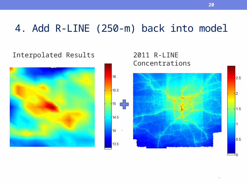
3. Spatial Bilinear Interpolation

CMAQ-OBS – R-LINE12km_av Interpolated Results

20

4. Add R-LINE (250-m) back into model

2011 R-LINE ConcentrationsInterpolated Results

21

2005 Annual Average PM2.5 Results

μg/m3

22

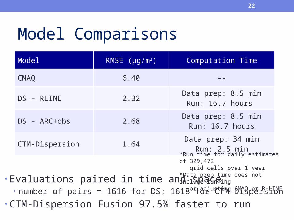
Model Comparisons

• Evaluations paired in time and space• number of pairs = 1616 for DS; 1618 for CTM-Dispersion

• CTM-Dispersion Fusion 97.5% faster to run

Model RMSE (µg/m3) Computation Time

CMAQ 6.40 --

DS – RLINE 2.32Data prep: 8.5 minRun: 16.7 hours

DS – ARC+obs 2.68Data prep: 8.5 min

Run: 16.7 hours

CTM-Dispersion 1.64Data prep: 34 min

Run: 2.5 min

*Run time for daily estimates of 329,472 grid cells over 1 year*Data prep time does not include running or adjusting CMAQ or R-LINE

23

Conclusions (CTM-Dispersion Model Fusion )

• Data fusion of CMAQ and R-LINE successfully created spatially resolved exposure estimates. Daily estimates will be used for a spatially-resolved birth cohort study in Atlanta from 2002-2010

• This approach can be applied to any pollutant with CMAQ and R-LINE estimates and any CMAQ grid size ≤ 12km

• Evaluation statistics depend heavily on performance of input estimates (better at roadways)

• This approach is much faster than the statistical downscaler

24

Acknowledgments• Collaborators at Georgia Tech and Emory University

*This publication was made possible by US EPA grant R834799. This publication’s contents are solely the responsibility of the grantee and do not necessarily represent the official views of the US EPA. Further, US EPA does not endorse the purchase of any commercial products or services mentioned in the publication.

Southeastern Center for Air Pollution & Epidemiology (SCAPE)www.scape.gatech.edu

Josephine Batesjbates2019@gatech.edu

THANKS!