GO-SHIP Repeat Hydrography Nutrient Manual, 2019:

The precise and accurate determination of dissolved inorganic nutrients in seawater;

Continuous Flow Analysis methods and laboratory practices.

Susan Becker1, Michio Aoyama2, E. Malcolm S. Woodward3, Karel Bakker4, Stephen Coverly5, Claire

Mahaffey6 Toste Tanhua7

1. UC San Diego, Scripps Institution of Oceanography 9500 Gilman Dr. MC 0236 San Diego CA 92093

2. RCGC, JAMSTEC/IER, Fukushima University, Japan

3. Plymouth Marine Laboratory, Prospect Place, The Hoe, Plymouth, PL1 3DH. United Kingdom

4. Royal Netherlands Institute for Sea Research, Department of Ocean Science, and Utrecht University, PO Box 59

Den Burg 1790 AB, The Netherlands

5. BLTEC, #1607, 1 Dong, 775, Gyeongin-Ro Yeongdeungpo-Gu, Seoul, 150-972, Korea

6. Department of Earth, Ocean and Ecological Sciences, SOES, University of Liverpool, Liverpool, L69 3GP. United

Kingdom

7. GEOMAR, Helmholtz Centre for Ocean Research Kiel, Duesternbrooker Weg 20, D-24105 Kiel, Germany

Table of Contents:

1. Introduction

1.1 Nutrient Data Comparability: GEOSECS to GO-SHIP

1.2 Methods and Instrumentation

2. Sample Collection and Storage

2.1 Sample collection

2.2 Filtering and gloves

2.3 Sample Preservation

3. Instrumentation

3.1 Sampler

3.2 Pump

3.3 Manifold

3.4 Detectors

3.5 Software

4. Measurement and concentration determination

4.1 Baseline determinations

4.2 Calibration

4.3 Measure sample peak heights

4.4 Corrections

4.5 Calculate initial sample concentrations

4.6 Post processing corrections

5. Methods

5.1 Nitrate and Nitrite Analysis

5.2 Phosphate Analysis

5.3 Silicate Analysis

5.4 Ammonia Analysis

6. Standards and Standardization

6.1 Primary standards

6.2 Secondary standards

6.3 Working standards

7. Quality Control and Quality Assessment (QC/QA)

7.1 Definitions and Determination of accuracy and precision

7.2 Standard Operating Procedures (SOPs)

7.3 Internal Checks: duplicates, check samples and tracking Standards

7.4 External Checks: use of Reference Materials and/or Other QC Samples

7.5 Data Comparisons

8. Documentation

8.1 Cruise reports, Metadata,

8.2 Bottle data files

References

Appendices

A: Applying air buoyancy corrections

B: Gravimetric calibration of volume contained in volumetric flasks and pipettes using water

C: Establishing the linearity of standard calibrations

D: Low-level (nano-molar) nutrients

E: Determination of nutrient concentrations in LNSW

F: Detailed methods utilized at SIO for AA3

G: Detailed JAMSTEC methods for QuAAtro

H: Experimental results: NIOZ and SIO sample freezing and thawing on silicate results

GO-SHIP Repeat Hydrography Nutrient Manual:

The precise and accurate determination of dissolved inorganic nutrients in seawater; Continuous Flow

Analysis (CFA) methods and laboratory practices.

1. Introduction

1.1 Nutrient Data Comparability: GEOSECS to GO-SHIP

The availability of inorganic macronutrients (nitrate (NO3), phosphate (PO4), silicic acid (Si(OH)4), ammonium (NH4), and nitrite

(NO2)) in upper ocean waters frequently limits and regulates the amount of organic carbon fixed by phytoplankton, thereby

constituting a key control mechanism of carbon and biogeochemical cycling. There are a number of biogeographic regions in the

open ocean characterized by different macronutrient regimes, either permanently or seasonally limiting the growth of

phytoplankton (Moore 2016). Accurately measuring temporal changes in macronutrient concentrations is essential to constraining

net biological production and export fluxes, detecting shifts in biogeographic regimes, and for monitoring eutrophication

phenomena. For open ocean work an accuracy of 1% should be aimed for by the GO-SHIP program (e.g. Talley et al., 2015) in

order to be able to quantify decadal trends in the deep ocean. An internal consistency of nutrient data in the order of 1to 3% has

been achieved through secondary quality control (QC) procedures implemented in GLODAPv2 (Olsen et al., 2016).

The Geochemical Ocean Sections Study (GEOSECS) in the 1970s was one of the first efforts to provide a global survey of

chemical, isotopic, and radiochemical tracers in the world’s oceans. Since then there have been numerous international

collaborations to map and study different chemical, physical, and biological aspects of the oceans. These programs include

JGOFS (late 80s), WOCE (mid to late 90s), and the current global programs CLIVAR, GEOTRACES, and GO-SHIP. In

addition to these large international efforts, there are many other programs being carried out by individual laboratories and

countries that studied, and continue to study, specific areas and processes in the world’s oceans, including ocean time-series

stations.

All of these efforts have led to large data synthesis studies, including CARINA, PACIFICA, GLODAPv1, and GLODAPv2.

These synthesis studies include analysis from different international laboratories. It is imperative that the data sets produced by

the different laboratories are comparable and differences in concentrations in time or space are real, and not artifacts of differing

methods, standards and instrumentation. In an effort to verify the comparability of the nutrient data sets there have been a

number of inter-laboratory comparability exercises (UNESCO 1965, 1967; ICES 1967, 1977; Kirkwood et al. 1991; Aminot and

Kirkwood 1995. There are commercially available nutrient standard solutions, eg. OSIL (http://osil.com/) and other programs

supply stock standards solutions that allow laboratories to validate their methods (Topping 1997). However, there is a need for a

reference material for nutrients that will allow laboratories to closely monitor and verify data quality.

There have been inter-laboratory comparison studies using reference materials with the first being NOAA/NRC MOOS-1 and

MOOS-2. The Meteorological Research Institute (MRI) in Japan has led the most recent series of international inter-laboratory

comparisons in 2003, 2006, 2008 and 2012 (Aoyama 2006, 2007, 2008, 2010). The motivation of the exercises led by MRI was

the development of reference materials for nutrients in seawater (RMNS). In 2014/2015 and 2017/2018 the International Ocean

Carbon Coordination Project (IOCCP) and Japan Agency for Marine-Earth Science and Technology (JAMSTEC) conducted

inter-laboratory comparison study of Certified Reference Material of Nutrients in Seawater and Reference Material of Nutrients

in Seawater. These two intercomparison exercises used CRMs as known samples (2014/2015) or as unknown samples

(2017/2018). The availability and use of these CRMS and RMNS has been instrumental in improving the global comparability of

nutrient data sets. These recent exercises were carried out as part of the terms of reference of the International SCOR working

group #147: Towards comparability of global oceanic nutrient data; (http://www.scor-int.org/SCOR_WGs_WG147.htm)

1.2 Methods and Instrumentation

The basic analytical methods and chemistries that are used to determine concentrations of inorganic nutrients in seawater are well

established. Strickland and Parsons outlined the manual methods in their book, “A Practical Handbook of Seawater Analysis”

(Strickland and Parsons 1972). The chemical methods have been changed, optimized and automated over the decades by

numerous authors, but the basic chemistries remain the same and are based on colorimetric reactions. The exception to this is the

newer methods for ammonia determination, which are based on fluorimetry.

Nitrate is determined using a procedure described by Armstrong (1967), which involves passing a seawater sample through a

copper-cadmium reduction column where the nitrate is reduced to nitrite. Nitrite is then diazotized with sulfanilamide and

coupled with N-(1-naphthyl)-ethylenediamine (N-1-N) to form a red azo dye, and the peak absorbance is between 520 and

540nm

Phosphate is determined by adding acidified ammonium molybdate to the seawater sample to produce phosphomolybdic acid,

which is then reduced to phosphomolybdous acid (a blue compound) following the addition of dihydrazine sulfate (Bernhardt

1967), or ascorbic acid (Murphy and Riley 1962), which was optimized by Zhang (Talanta 49 (1999) 293-304). The absorbance

is measured at ~850 – 880nm.

Silicate is analyzed according to Armstrong (1967) by producing a silicomolybdic acid with the addition of ammonium

molybdate. Silicomolybdous acid (a blue compound) is formed following the addition of stannous chloride, and the absorbance

is measured at ~660nm. An alternative method uses ascorbic acid (Grasshoff 1983) to reduce the silicomolybdic complex to a

blue compound, and the absorbance is measured at ~820nm.

There are two different ammonium methods. The colorimetric method uses the Berthelot reaction, and involves the reaction of

hypochlorous acid and phenol with ammonium in an alkaline solution to form indophenol blue. The sample absorbance is at

660nm. This method is a modification of the procedure by Koroleff (1969,1970). A highly sensitive fluorimetric method using

ammonia diffusion across a teflon membrane and fluorimetric detection was published by Jones (1991), but obtaining the

membrane proved difficult. A simplified sensitive technique using fluorimetry but without the use of a membrane, was published

by Holmes (1999), which was adapted from Kerouel and Aminot (1997). The seawater sample is combined with a working

reagent containing ortho-phthaldialdehyde, sodium sulfite, and borate buffer and heated to 75°C. Fluorescence proportional to

the ammonium concentration is emitted at 460nm following excitation at 370nm.

Laboratories started using Continuous Flow Analysis (CFA) and Auto-Analyzers (AA) in the mid-1970s. The two main forms of

CFA are flow injection (FIA) and gas-segmented analyzers. While there are some laboratories that are using FIA for nutrient

analysis, most global laboratories that carry out ‘at-sea’ analysis use gas-segmented flow analyzers. This manual focuses

primarily on methods for gas-segmented analyzers.

The chapter on nutrient analysis using segmented flow analysis by Aminot et al. (2009) in “Practical Guidelines for the Analysis

of Seawater” provides an excellent background on continuous flow analysis. We recommend the reader reviews this document as

it contains useful information on the technical aspects of the instrument(s), the measurement of nutrients, as well as details on

sources of error and contamination.

This GO-SHIP document reviews basic sample collection and storage, aspects of CFA using an Auto-Analyzer, and specific

nutrient methods in use by many laboratories doing repeat hydrography. The document also covers laboratory practices including

QC/QA procedures to obtain the best results and suggests protocols for the use of reference materials and certified reference

materials.

2. Sample Collection and Storage

2.1 Sample collection

Nutrient samples should be collected from the rosette/Niskin bottles immediately after the collection of samples for gases. This

can be challenging if samples for organic properties or biologically sensitive properties are also being taken.

Ideally, samples are collected into new, sterile plastic (HDPE, PP) containers that will then fit directly onto the AA sampler

carousel. However, using a new sample container can be costly and produces a tremendous amount of plastic waste on the long

repeat hydrography research cruises. Sample containers can be re-used if proper cleaning procedures are followed between

stations. For macro-nutrient analysis (micro-molar concentrations), rinsing the sample containers with distilled deionized water

followed by a rinse with 10% HCl (hydrochloric acid) is sufficient. This stops any biological growth in bottles. The bottles

should be rinsed well with deionized water prior to the collection of the next samples. Glass sample containers should not be used

due to silicate contamination. If nano-molar nutrient levels are being measured, other cleaning and sample collection procedures

will be necessary (see Appendix D).

When taking the seawater samples from the rosette, rinse the clean sample containers and caps three times before filling. Avoid

touching the sampling spigots on the Niskin bottles and take care to rinse the spigots as well as the nutrient sample containers.

Samples can be collected without the use of a Tygon or silicon sampling tube. If a sampling tube is used, rinse it thoroughly

before going out to the rosette to take a series of samples, and make sure to rinse it with each seawater sample prior to collecting

the sample. Between CTD sampling events it is important to clean any sampling tube with clean deionized water and 10% HCl.

Once rinsed then fill the sample containers two thirds full, and cap immediately. The samples should be analyzed as soon after

sample collection as possible. If analysis will be delayed for longer than a couple hours (1-2 hrs), then store the samples in the

dark and cool place, for example in a refrigerator, however the samples should be returned to room temperature before analysis.

Cigarette smoke can contaminate samples, particularly for ammonium and nitrate/nitrite, so it is imperative that smoking is

banned close to the area where samples are collected. Likewise people who have been recently smoking should stay away from

any open samples.

2.2 Filtering and gloves

Some laboratories filter nutrient samples, while many other laboratories do not. In general, filtering is not necessary for samples

taken in the (sub) tropical open ocean, where particle loading is low in these are oligotrophic environments. The decision to filter

or not is dependent on the particulate loading in the water being sampled. For example samples from near shore or productive

environments may require filtering. In these cases, great care must be taken not to contaminate the samples during the sample

handling and filtering process. Sample collection tubes, filter holders, and filters should be clean and well rinsed prior to sample

collection. Types of filters often used to filter seawater include cellulose acetate, hydrophilic polypropylene Gelman membrane,

and Acrodisc syringe filters. Glass Fiber filters (GFF) (silicate contamination) or cellulose nitrate filters (nitrate contamination)

should NOT be used. Filter size is another consideration. A pore size of 0.45µm filter is commonly used, and in the past this

was considered the ideal filter size to remove the majority of partilces. However new insight from microscopy and genomics has

received that a 0.45µm filter does not capture all bacteria and phytoplankton. Instead a 0.2µm filter is now the preferred size of

filter to be used. The flow rate through these filters is low and if filtration is done under pressure or high vacuum, there is a risk

of cell rupture and sample contamination. Gravity, low pressure, or low vacuum filtration is recommended. It is imperative that

tests are performed to check that the method of filtering, filter type, and size do not lead to contamination of the samples.

Gloves are another source of debate regarding possible contamination. Neither Neoprene or colored nitrile gloves should ever be

used in the lab or for sampling for nutrients; they are a high source of contamination especially for nitrate, nitrite and ammonium.

If care is taken, a clean sample can be collected with bare hands without the use of gloves. However, vinyl, powder-free, gloves

are recommended for use in the lab and for sample collection.

In general, it is good practice to wear gloves when taking water samples and only experienced scientists who are confident in

their techniques should consider sampling without gloves. Likewise it is important that any sampling procedures (like gas

sampling) being carried out prior to the nutrient sampling from the CTD, then those scientists should also wear non-nutrient

contaminating gloves.

2.3 Sample Preservation

There are many instances when nutrient analysis at sea is not possible or is delayed for any number of reasons. If analysis will be

delayed by more than 24 hours the samples must be preserved. There are many different types of preservation methods,

including poisoning, acidification, pasteurization (Daniel et al. 2012), and freezing. We do not recommend poisoning samples

with mercuric chloride or by acidification. Freezing is the most commonly used method, and there are studies that show that

freezing can be a reliable method of sample preservation (Aminot 1995; Dore et al. 1996).

It is imperative that frozen seawater samples have sufficient head space in the bottles to allow for expansion during freezing.

Freeze the samples upright and check that the caps are tightened before and after the samples have frozen. Do not freeze samples

in a freezer that has had organic material (fish samples or food) stored in it. Analyze frozen samples as soon as possible after

returning to the lab.

There is still debate within the nutrient community about the effects of freezing samples on the accuracy and precision of the

nutrient concentration, especially for silicate. It is well known that the reactive silica polymerizes when frozen, especially at high

concentrations (Burton et al. 1970; MacDonald et al. 1982; MacDonald et al. 1986). Much of the current debate centers on the

proper thaw techniques to depolymerize the reactive silica to get complete recovery. Many laboratories have done studies of

thaw techniques to recover silica, but there are only a few published references. Sakamoto et al. (1990) recommend that samples

be thawed overnight in the dark at room temperature or thawed in a water bath for 30 minutes and then cooled back down to

room temperature before actual analysis. Zhang and Ortner (1998) suggest that it can take up to 4 days to thaw samples at room

temperature to get complete recovery of silica. Recent tests done at the Royal Netherlands Institute for Sea Research and Scripps

Institution of Oceanography confirm the 1990 recommendation by Sakamoto of thawing frozen samples in a 50 degree C water

bath for 30-45 minutes and then allowing the samples to come back to room temperature before analysis (Appendix H).

Variables, which affect the recovery of silica from frozen samples, include salinity, turbidity, and silica concentration. The

nutrient community and authors of this manual are carrying out systematic tests to determine the best thaw techniques for the

types of samples being collected (coastal, estuarine, oligotrophic, etc), some initial results are presented in appendix H.

3. Instrumentation

Aminot et al. (2009) provide a detailed description of the specific AA components, including potential problems.

Most seagoing laboratories are using SEAL (AA3), Skalar, Alpkem, or similar analytical systems. Users should refer to the

manufacturer's manuals that came with the instrument for the specifics on methods, operation, and maintenance. A nutrient auto-analyzer from any manufacturer will consist of the same basic components listed and described here.

3.1 Sampler

The sampler should be robust and able to handle different size sample cups, and a number of samples. It should have a

continuously refreshed wash station. A non-metallic or platinum probe should be used, and the internal diameter of the probe

should normally be no greater than that of the largest sample pump tube. Having a sampler modified to accept the bottles that you

sample straight from a CTD for example will eliminate possible contamination issues if decanting a sample into another sampling

vessel.

3.2 Pump

The peristaltic pump(s) delivers the sample/baseline water and the reagents to the manifolds for each channel/chemistry and

throughout the entire AA system. For precise measurements at low concentrations, a regular bubble pattern and stable baseline

are absolutely key, and this is one area that is extremely important to get correct for good analyses.

The composition and quality of pump tubes can vary between manufactures and from batch to batch. Replacing a method’s

pump tubes may improve the sensitivity and bubble flow. Wear will also affect the tube’s flow rate and method sensitivity,

which is why a complete set of standards should be run with every station/set of samples. Consult the operations manual of

individual instruments for the recommended frequency to change out pump tubes, however generally pump tubes should be

changed on a regular basis as the correct delivery of the sample, and particularly for some reagents being pumped through some

of the smaller bore pump tubes (eg: orange/green or orange/yellow), will become a lot less accurate as the tubes wear. For

optimum performance then changing tubes after between 60-80 hours of use will ensure that the liquid delivery remains reliable.

It is a false economy to run pump tubes right to the end of their useable life as the results will not be as good or reliable as with

newer tubes. Some laboratories make a full change of pump tubes and reagents at the same time to co-ordinate machine down

time.

3.3 Manifold

The manifold consists of glassware and injection fittings and is the site of the chemical reactions between the seawater samples

and reagents. It is imperative that the glass pieces, reaction coils, and connectors are maintained regularly in order to provide

consistent mixing and flow and to allow reactions to reach steady state and ensure a full color development.

Introduction of air (or nitrogen) bubbles allows for complete mixing between segments and maximizes color development. The

bubbles must be large enough to prevent carryover and/or smearing from one segment to another but not too long, which makes

them prone to breaking up in the manifold. It is very important to maintain a regular bubble pattern throughout the system in

order to reduce noise and optimize sensitivity. Reference is always made to the segmented gas bubbles as being ‘air’ bubbles,

however ideally these segmenting bubbles should be either nitrogen or another inert gas so as to avoid potential contamination

from the air. Some laboratories have gas lines direct from cylinders to deliver the gas, but a simpler solution is to use small

plastic Tedlar bags (or similar) that contain up to 5 litres of nitrogen that can be easily refilled. These are particularly useful when

working at sea.

There are many factors to consider when building a manifold to ensure consistent flow and bubble pattern. Below is a list of

considerations:

1. Match the inner diameter (ID) of the tubing used from the pump to the injection fittings and into the glassware on the

manifold as closely as possible.

2. Use the shortest possible length of tubing between connections. Long un-segmented streams can cause hydraulic

problems, which will manifest in various ways (e.g. smearing or carryover of samples).

3. Make sure there are no gaps/dead spaces between connections. It is important that all glass to glass joints a held close

together by plastic sleeving.

4. Add enough wetting agent in each flow to maintain rounded edges at the front and back of each bubble throughout the

entire flow stream, including the drain to waste.

5. Bubbles must completely fill the tubing through which they pass. The length of bubble in contact with the tubing walls

should be 1 - 1.5 times the tubing diameter.

6. Maintain the cleanliness of the glass coils to maintain flow. Dirty glass can cause bubbles to stick or break up.

7. Clean the manifolds periodically with a a phosphate-free laboratory detergent. A dilute bleach or acidic solution can

also be used. Consult the instructions for your particular instrument for the cleaning frequency and solution.

8. The segmented flowcell waste line should open to the atmosphere at about bench or flowcell height

9. Replace any glass pieces that continue to cause the air bubbles to stick or break up.

3.4 Detectors

The detectors consist of a light source (eg: lamp, LED ), flowcell, photometer and inlet and outlet tubing (either plastic or glass).

As with the manifold, there should be no gaps at the connections, and there should be regular bubble pattern maintained from the

manifold through the detector unit to waste. Depending on the manufacturer, the ability to monitor changes in light output,

voltage, and other variables through the software may be available, and should be utilized. In the past the sample flow was

always debubbled immediately prior to the sample entering the flowcells, but now software developments have allowed the air

bubbles to also pass through the cells eliminating the need to debubble. The optical design of the new photometers and flowcells

have nearly eliminated the need for refractive index blanks (RIB) and some other effects that have interfered with peak detection

in the past. For more details on these corrections see section 4.6.

3.5 Software

The AA will come with software from the manufacturer to control the entire system, program the autosampler, acquire the raw

data output from the detectors, display the output real-time, and perform some corrections and calculate initial concentration

values.

There are usually different options for the calibration fit to use within the software packages. If using a linear fit or higher order

fit the concentration of nutrients in the matrix, and the blanks for the matrix and the samples, must be carefully determined and

corrected for. Most software programs will correct for carryover, baseline, and sensitivity drifts but may not have options to make

other corrections such as refractive index blanks or non-zero matrix concentrations. Please refer to the software manual for your

own type of analyzer to learn the specifics for your instrument.

Calibration fits and blank corrections are discussed in more detail later (Appendix C).

4. Measurement and determination of nutrient concentrations:

The basic steps for sample analysis include:

1) Baseline determinations for ultrapure water (distilled deionized water, MilliQ, Nanopure, or equivalent) and ultrapure water

plus reagents.

2) Calibration curve determination from standard concentrations and measured peak heights.

3) Measurement of sample peak heights.

4) Corrections to peak heights for any baseline drift, sensitivity drift, and carryover.

5) Determination of initial concentrations of samples based on calibration curve and sample peak heights.

6) Application of other corrections including RI blanks, salt effect, etc.

4.1 Baseline determinations

The common baseline solution used throughout the nutrient analysis community is ultrapure fresh water. However in some cases

analysts use low nutrient seawater (if they have plentiful supplies) and some labs make their own ‘artificial’ seawater by adding

salts to ultrapure water. Here is an example of one recipe for ASW,:

41g of NaCl and add 2mM or HCO3- or 168mg NaHCO3 per liter. Here we will discuss using ultrapure water as the baseline

water as this is a reliable ‘zero’ for nutrients and can be obtained easily and quickly within a research laboratory.

Determination of the baseline should be straightforward if the correct procedures are followed. The ultrapure water should be at

least 18.2 megohm resistance, and be free of organics. Ultraviolet (UV) sterilization is preferred but not strictly necessary. Most

commercially available water purification systems (e.g. MilliQ, Nanopure, Aquapure) will provide ultrapure water that is

acceptable for establishing a zero baseline. The wash pot on the sampler and the container that feeds into the wash pot can

become contaminated with nutrients. These should be cleaned once per day. Some manufacturers offer a ‘travelling washpot’

which is a sealed system and hence stays uncontaminated and clean during daily operations so could be an option to consider. In

rare cases it is possible that the ultrapure water is not pure, even if the resistivity reading is 18.2 megohm. One indicator of poor

quality baseline water is negative absorbance readings samples with a low nutrient concentration.

The water baseline is determined after the instrument has been running long enough with fresh ultrapure water and the baselines

are stable. It may be necessary in rare cases to add wetting agent to the ultrapure water to establish a good bubble pattern and

stable baselines. Once the ultrapure water baseline has been established, the reagents can be added and the reagents plus

ultrapure water baseline established. It is often useful to add the reagents one at a time if a large reagent blank has been noted, or

for other troubleshooting. The reagent baseline is the reference when the standard curve is determined and subsequent

calculation of sample concentration. It is good practice to establish a regular setting up process for the analyser that can be

followed for every day and every run.

To minimize the reagent blank, analytical grade (or better) chemicals and fresh ultrapure water should be used. The reagent

blank is the difference between the ultrapure water baseline and the reagent baseline after all the reagents are online.

It is crucial that the nutrient concentrations for low nutrient seawater (LNSW) or artificial seawater (ASW) are calculated if they

are being used as a baseline instead of ultrapure water. Aoyama et al. (2015) detail a procedure which includes analyzing a

known value of each standard added to the LNSW, followed by a baseline of LNSW with and without color reagent, and a

baseline of distilled water with and without reagent. The differences are used to calculate the concentration of each nutrient in

LNSW. See Appendix E for details.

There are different ways to obtain low nutrient seawater (LNSW). One option is to collect large batches of surface seawater from

oligotrophic waters during a research cruise. It is recommended that the water be filtered and sterilized to ensure the nutrient

levels remain low, e.g. pumped through a 0.45µm filter, past a UV light source, and then through a 0.1µm filter, and recirculated

for a total of ~16 hours. Alternatively, it is possible to collect seawater, remove grazers using a 0.1/0.2 m filter and then allow

the seawater to age, stored at room temperature for some period of time (1-2 years), allowing the already oligotrophic water

nutrient concentrations to decrease over this time period. The carboys used to store the seawater should allow light penetration

(clear or opaque).

4.2 Calibration

A series of at least four working standards should be analyzed with every set of samples. The standard concentrations should be

evenly distributed over the entire concentration range and not skewed toward either end, with the top concentration standard

having a higher concentration than the highest sample. Standards are generally analyzed at the beginning of an analytical run

with the protocols set up on the analyzer software. Working standards should be prepared fresh at least once a day, or every 8 to

12 hours when the nutrient analyzer is in operation 24 h a day, e.g. when working at sea. Working standards are prepared from

concentrated secondary or primary standards that are pre-made in ultrapure water (see section 6 for standard preparations). For

the working standard curve, the concentrated standards are diluted using water that has a similar matrix to the samples. For

example using aged low nutrient seawater or from the surface waters if working in an oligotrophic ocean region can be used as

the standard martrix. The standard curve should cover the full range of expected sample concentrations. It is important that

LNSW be used for the dilutions (see section 4.1). Once the peak heights from the standards have been measured, then the

calibration curve can be produced. Analytical software form the instrument manufacturers will supply this with modern

analyzers so see their guidance notes for details. See Appendix C for details on how to determine the correct calibration fit.

4.3 Measure sample peak heights

Most software uses an algorithm to determine the peak height and will automatically place a peak marker where it considers the

correct peak height should be. However, the computer readouts should always be checked for spikes and other anomalies that

may affect the validity of the initial value, with adjustments made as necessary within the software package. Refer to the

software manual for details on how the peaks are measured and how to adjust and save the readings if needed.

4.4 Corrections

Carryover is based on the difference of peak heights between two successive low peaks measured directly following a high peak.

Baseline drift accounts for any linear drift between successive baseline measurements, which should be placed throughout the

run. Sensitivity is measured by any linear change between “drift” samples, which are analyzed near the beginning and end of the

run, if not more frequently.

4.5 Calculate initial sample concentrations

Most software has the option of applying baseline, carryover and drift corrections, and can give both corrected and uncorrected

sample concentrations. It is recommended that users review how the calculations are applied to ensure the validity of any post-

run corrections. It may be necessary to output the raw data to apply corrections and calculate concentrations.

4.6 Post processing corrections

Refractive index blanks (RIB) assign a value to samples with a concentration of zero, and can be subtracted from actual sample

concentrations. The procedure for determining these values for each analytical chemistry involves analyzing samples with

different RIB reagents, which involves removing one or more of the color forming reagent chemicals (Aminot et al. 2009). For

many systems, these values are usually positive, though negligible, but should be determined and then any corrections measured

are necessary to be applied to the results before the sample concentrations are finalized. In fluorimetric methods, such as for

ammonia, no RIB is produced.

New detectors minimize the effects of salinity on the analysis of seawater samples and a correction isn’t necessary. For older

instruments, see Aminot et al. (2009) for the procedure.

Likewise, the Schlieren effect, which is present when a distilled water wash is used to separate seawater samples, is reduced in

newer systems by flowcells and detectors that allow the inter-sample bubble to pass through. Use of a debubbler before the

flowcell increases the Schlieren effect, leading to tails on peaks of lower concentration, and should thus be avoided (Aminot et al.

2009).

5. Chemical analytical Methods

Analytical methods, including reagent recipes and coil configurations, are supplied from the manufacturers of all AA

instruments. They can and should be used reliably. Some laboratories have optimized methods for their own use and are often

passed down over many years through different analysts. One reason to optimize/change methods is to allow for greater

sensitivity at lower nutrient concentrations if working mostly in oligotrophic waters. See Aminot 2009 and Appendix F for

detailed methods in use by some specific laboratories. These are only supplied as examples to allow comparison with local

methods and reagent recipes.

5.1 Nitrate and Nitrite Analysis

Most laboratories are using a method where N-(1-Naphthyl) ethylenediamine dihydrochloride (known as N-1-N or NEDD) and

sulfanilamide are reacted with the sample to form a red dye which is measured at an absorbance of 520-540 nm. For the nitrate

analysis the sample is first mixed with a buffer solution and passed over a cadmium column that has been treated with copper

sulfate, which catalyzes the reduction of nitrate to nitrite. The resulting Nitrite is then analyzed and so the final output for the

‘Nitrate’ channel is a sum of both Nitrate and Nitrite.

The efficiency of the cadmium column should be determined and tracked over time. Two standards are prepared, one with a high

concentration of nitrate and the other with the same concentration of nitrite. A dilution of secondary standards can be used for

this purpose. The difference in these values gives the column efficiency. If the column efficiency is lower than 95%, the

cadmium column should be reconditioned, but if this does not regenerate the column then it should be replaced.

5.2 Phosphate Analysis

There are two commonly used methods for phosphate determination. With both, an acidic solution of molybdate is added,

followed by the addition of a reducing compound (dihydrazine sulfate or ascorbic acid) to form phosphomolybdous acid (a blue

compound), and absorbance measured at ~820 or 880nm depending on the method.

5.3 Silicate Analysis

As with phosphate, there are two commonly used methods for silicate determination. Acidified ammonium molybdate is added

to a seawater sample to produce silicomolybdic acid, which is then reduced to silicomolybdous acid (a blue compound) following

the addition of stannous chloride or ascorbic acid, and measured at 660 or 820nm depending on the method.

NB: It is important to ensure the Silicate and Phosphate methodologies have the correct reagent chemistry make ups, eg: the

Phosphate reactions should take place at a pH of <1.0, this is to ensure there is no competitive reaction from Silicate ions. eg:

Oxalic or Tartaric acids are used to prevent phosphate interferences in the silicate methods. Some methods with incorrect

chemistries can have cross contamination and hence incorrect Phosphate and Silicate concentrations reported.

5.4 Ammonia Analysis:

The two common methods for determining ammonia concentrations are the phenol based colorimetric determination and a

fluorometric method.

Colorimetric method:

Ammonium is analyzed via the Berthelot reaction in which hypochlorous acid and phenol react with ammonium in an alkaline

solution to form the indophenol blue complex. The sample absorbance is measured at 640nm. The method is a modification of

the procedure by Koroleff (1969,1970).

Fluorometric method:

In the fluorometric method, without using any membrane diffusion, the sample is combined with a working reagent made up of

ortho-phthalaldehyde, sodium sulfite, and borate buffer and heated to 75°C. Fluorescence proportional to the NH4 concentration

is emitted and measured at 460nm following excitation at 370nm.

6. Standard Preparation and Standardization

It is important to determine the exact concentration of standard solutions, taking into account buoyancy corrections, glassware,

and pipette calibrations, and temperature corrections (Appendices A and B).

Glass Volumetric flasks, when being used, should be of Class A quality because their nominal tolerances are 0.05 % or less over

the size ranges. Class A flasks are made of borosilicate glass, and the standard solutions should be transferred to plastic bottles as

quickly as possible after they are made up to volume and well mixed in order to prevent excessive dissolution of silicate from the

glass. PMP volumetric flasks should be gravimetrically calibrated and used only within 4 K of the calibration temperature.

The computation of volume contained by glass flasks at various temperatures other than the calibration temperatures are carried

out by using the coefficient of linear expansion of borosilicate crown glass.

Because of their larger temperature coefficients of cubical expansion and lack of tables constructed for these materials, the plastic

volumetric flasks should be gravimetrically calibrated over the temperature range of intended use and used at the temperature of

calibration within 4 K. The weights obtained in the calibration weightings are corrected for the density of water and air buoyancy.

Pipettes and pipettors

All pipettes whether they are manual or electronic must be regularly calibrated according to the manufacturers recommendations

and should be within the tolerances as stated. Calibration can be carried out by the analyst or by commercial companies who will

provide certificates. Certainly before going on a research cruise the pipettes should have their calibrations checked, and also at

regular times during the year. If pipettes are dropped they should be calibrated before being used for making analytical solutions.

Pipettes normally have calibration tolerances of 0.1 % or better. These tolerances should be checked with gravimetric calibration.

6.1 Primary Standards

Primary standard-grade salts for phosphate (anhydrous potassium dihydrogen phosphate, KH2PO4), nitrate (potassium nitrate,

KNO3) and nitrite (Sodium Nitrite, NaNO2) are available with purities of 99.995% or better. No corrections for purity are needed

if these salts are used when preparing primary standards. . Silicate standards are made with analytical grade sodium

hexafluorosilicate or from a silica standard solution (SiO2). Ammonia standards are made with analytical grade ammonium

sulfate (NH4SO4), which is available with purity of >99.0%. The purity of the salt or solution used for the primary standards in

these cases should be adjusted as appropriate and clearly stated in the documentation. Care must be taken to neutralize the silica

standard solution if it is prepared in dilute sodium hydroxide.

The powder or salts should be dried for 2 to 4 hours at 105°C and completely cool in a desiccator. The salts should be weighed

out to a precision of 0.1mg, and the exact weight recorded. Dissolve the standard salts in ultrapure water and record the

temperature of the solution. Use Class A volumetric flasks should be used and the calibration (Appendix B) periodically checked

(~once/year).

Adjust the weight of the salt for a buoyancy correction (Appendix A) when determining the exact final concentration of the

primary standard solutions.

The following examples of primary standard preparation are supplied here only as a guide. You should record the temperature of

the final solutions and calculate the concentration of the primary standard using the volumetric flask volume, temperature, and

the true mass of powder. Eash soliution should bet ransfered each solution to a clean, dry HDPE bottle and stored ready for use.

It is very important that Silicate standards should never be stored in glass.

Nitrate Standard (~15,000 micro-mole/L):

In a 1 liter calibrated class A volumetric flask, dissolve ~1.5xxx g of high purity dried KNO3 in ultrapure water to make a 1 liter

final volume solution.

Nitrite Standard (~5,000 micro-mole/L):

In a 1 liter calibrated class A volumetric flask, dissolve ~0.34xx g of high purity dried NaNO2 in ultrapure water to make a 1 liter

final volume solution.

Phosphate Standard (~6,000 micro-mole/L):

In a 1 liter calibrated class A volumetric flask, dissolve ~0.81xx g of dried high purity KH2PO4 in ultrapure water to make a 1

liter final volume solution.

Ammonium Standard (~ 4,000 micro-mole/L):

In a 1 liter calibrated volumetric "A" flask, dissolve ~0.26xx g of dried high purity (NH4)2SO4 in ultrapure water to a 1 liter final

volume solution.

Silicate Standard: (10, 000 µmole/L (=10mmole/L))

In a 1L HDPE plastic volumetric, dissolve 1.8806g of sodium fluorosilicate in about 700mls of ultrapure water. This will take a

minimum of 5 hours to dissolve using ultrasonics or by stirring. In all cases clean protocols must be adhered to. Make the

dissolved solution up to 1 Litre with ultrapure water. Add 300µl of chloroform as a preservative.

Alternative commercial Liquid silicate standard:

Add 90.13ml of a 1000 ppm sodium metasilicate nonahydrate solution to 1L of secondary standard for a 1,500 micro-mole/L

concentration. Add 180.25mL to 1L of secondary standard solution for a 3,000 micro-mole/L concentration.

NB: If the commercial silicate solution used is alkaline then care must taken to neutralize the final solution.

6.2 Secondary (Sub-primary) Standards

Depending on the desired concentrations for the final working standards, either separate nutrient standards, or a mixed secondary

standard can be prepared by diluting the primary standards with ultrapure water. A secondary solution for nitrate, phosphate, and

silicate can be made up at the same frequency as the primary standards. The secondary standard for nitrite and ammonia should

be made up each time there is the requirement also for a set of working standards, ie: every analytical run. The final concentration

of the secondary standards should take into account glassware and pipette calibrations (see Appendix B).

6.3 Working standards

Working standards are made up in LNSW, ASW, or in the water matrix/same salinity water as the samples if LNSW and ASW

are not available. These are prepared from the secondary, or primary solutions, depending on what the desired final

concentrations are. At least four different concentrations of working standards should be analyzed with every station/set of

samples.

7. Quality Control and Quality Assessment (QC/QA):

7.1 Definitions and Determination

Quality control procedures and quality assessment of the data provide means to determine the accuracy and precision of the

measurements.

Definitions are provided, as it is important that the analyst understand the difference between quality control, quality assessment,

accuracy, and precision. From Chapter 3 of “Guide to Best Practices for Ocean CO2 Measurement” (Dickson 2007):

Quality control — The overall system of activities whose purpose is to control the quality of a measurement so that it meets the

needs of users. The aim is to ensure that data generated are of known accuracy to some stated, quantitative degree of

probability, and thus provides quality that is satisfactory, dependable, and economic.

Quality assessment — The overall system of activities whose purpose is to provide assurance that quality control is being done

effectively. It provides a continuing evaluation of the quality of the analyses and of the performance of the analytical system.

Precision is a measure of how reproducible a particular experimental procedure is. It can refer either to a particular stage of

the procedure, e.g., the final analysis, or to the entire procedure including sampling and sample handling. It is estimated by

performing replicate measurements and estimating a mean and standard deviation from the results obtained.

Accuracy, however, is a measure of the degree of agreement of a measured value with the “true” value. An accurate method

provides unbiased results. It is a much more difficult quantity to estimate and can only be inferred by careful attention to

possible sources of systematic error.

7.2 Standard Operating Procedures (SOPs)

Quality control begins with setup of the instrument and attention to details in the manifold assembly and maintenance that are

outlined in section 3.3 of this manual. Once the instrument is set up and running a set of standard operating procedures should be

put in place and followed for the analysis of the samples.

The SOPs should include:

• Calibration of glassware and pipettes (Appendix B).

• Careful determination of standards and calibration fits (section 6 and Appendix C).

• Daily checks on the system, including visual inspection of bubble patterns, tracking the baseline with and without

reagents, and a test sample (usually a high standard) to ensure everything is working properly and to the same settings and

sensitivities as previously obtained for that test sample. This is also a broad good quality control measure in that for

example for the same test sample concentration then the analyzer sensitivity (gain) settings should stay the same, even

after changing reagents or pump tubes. If it changes it is an early indication that there is a problem that needs to be

investigated, probably associated with whatever changes have been made (eg: a reagent has been incorrectly prepared,

incorrect pump tubes replaced).

• An established tray protocol in the software, see example in Figure 1 below. This is used to ensure standards, samples,

and other peaks are included and run in the same order for each analysis. It can include carryover, drift, baseline, and

other corrections.

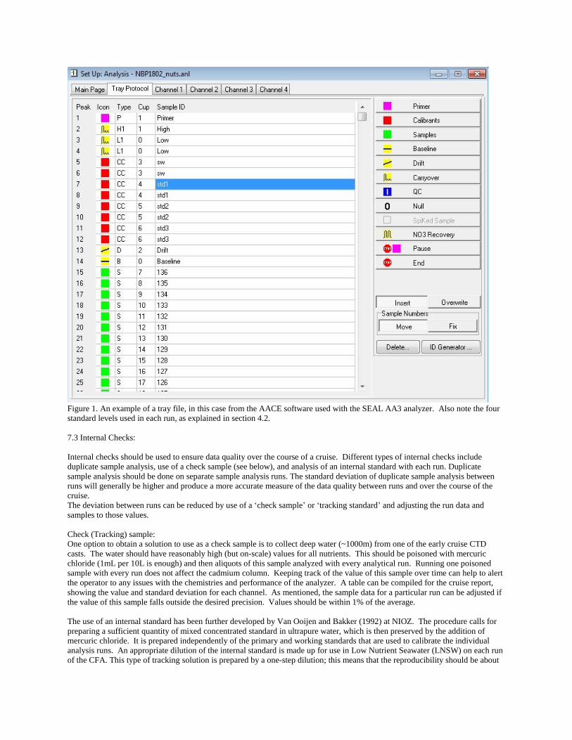
Figure 1. An example of a tray file, in this case from the AACE software used with the SEAL AA3 analyzer. Also note the four

standard levels used in each run, as explained in section 4.2.

7.3 Internal Checks:

Internal checks should be used to ensure data quality over the course of a cruise. Different types of internal checks include

duplicate sample analysis, use of a check sample (see below), and analysis of an internal standard with each run. Duplicate

sample analysis should be done on separate sample analysis runs. The standard deviation of duplicate sample analysis between

runs will generally be higher and produce a more accurate measure of the data quality between runs and over the course of the

cruise.

The deviation between runs can be reduced by use of a ‘check sample’ or ‘tracking standard’ and adjusting the run data and

samples to those values.

Check (Tracking) sample:

One option to obtain a solution to use as a check sample is to collect deep water (~1000m) from one of the early cruise CTD

casts. The water should have reasonably high (but on-scale) values for all nutrients. This should be poisoned with mercuric

chloride (1mL per 10L is enough) and then aliquots of this sample analyzed with every analytical run. Running one poisoned

sample with every run does not affect the cadmium column. Keeping track of the value of this sample over time can help to alert

the operator to any issues with the chemistries and performance of the analyzer. A table can be compiled for the cruise report,

showing the value and standard deviation for each channel. As mentioned, the sample data for a particular run can be adjusted if

the value of this sample falls outside the desired precision. Values should be within 1% of the average.

The use of an internal standard has been further developed by Van Ooijen and Bakker (1992) at NIOZ. The procedure calls for

preparing a sufficient quantity of mixed concentrated standard in ultrapure water, which is then preserved by the addition of

mercuric chloride. It is prepared independently of the primary and working standards that are used to calibrate the individual

analysis runs. An appropriate dilution of the internal standard is made up for use in Low Nutrient Seawater (LNSW) on each run

of the CFA. This type of tracking solution is prepared by a one-step dilution; this means that the reproducibility should be about

0.1% due to the inherent errors of pipetting. Note: The use of this tracking solution is only allowed if its value is in the same

range as the samples in the field, and in a range of about 60-80% of full scale values.

The tracking solution is diluted in LNSW and measured in between the samples as part of each analysis run. At the end of the

cruise, a mean value for the tracking solution or the check sample is calculated and the data for each run can be adjusted to the

mean value by calculating and applying a factor for each run.

The tracking solution or check sample should be analyzed multiple times within one analysis run to monitor performance within

each run as well as between runs, over the course of the cruise. These internal checks can be used to normalize data for each

station. At the end of the cruise the a mean value for the internal check is calculated and the data for each run is adjusted by the

ratio of value for the internal check on that run to the mean value for the whole cruise.

7.4 External Quality Checks:

External checks help assess the comparability of data from different cruises and laboratories. Participation in national or

international inter-comparison (intercalibration) exercises are one example of an external check. Another recommended external

check is to include the analysis of Certified Reference Materials (CRMs), or reference materials (RMs), within an analytical run.

CRMs and RMs are preserved seawater samples with well-defined nutrient concentrations that are used to ensure consistency of

measurements within a cruise (i.e. station to station; after new batch of reagents or standards has been prepared etc.), and between

different cruises, most likely executed by different laboratory groups. CRMs can be obtained in various concentrations and with

various seawater matrices, representing various ocean conditions/salinities. It is strongly recommended to use nutrient CRMs for

all research cruises and for lab analysis, especially so for cruises and data where high accuracy is required, such as for the repeat

hydrography programs GO-SHIP (CLIVAR) and GEOTRACES.

Reference Material for Nutrients in Seawater (RMNS) have been developed and produced in recent years by KANSO Technos.

The SCOR Nutrient working group #147 (http://www.scor-int.org/SCOR_WGs_WG147.htm) in association with JAMSTEC,

have had produced a series of 5 sets of RMNS, with 2 Pacific and 3 Atlantic concentration range solutions now being available to

the global nutrient community. These are sold on a non-profit basis to benefit the community and to encourage a wider use of

CRM’s. They are available for purchase through JAMSTEC (https://www.jamstec.go.jp/scor/), and have been produced in order

to make the use of the RMNS cheaper and hence more accessible to a greater number of global laboratories. These come in 100

mL plastic containers, which can be opened and transferred to clean sample tubes and analyzed with every run, or at least once

per day. The nutrient analytical values should be tracked so that any changes are noted and investigated. There are other

manufacturers of the RMNS, eg. Korea, Eurofins.

The certified values of SCOR-JAMSTEC CRMs and KANSO CRMs are traceable to the International System of Units (SI)

through an unbroken chain of calibrations. For nitrate, nitrite and phosphate values, Japan Calibration Service System (JCSS) of

Chemicals Evaluation and Research Institute (CERI) and the National Metrology Institute of Japan (NMIJ) standard solutions

with stated uncertainties are used. For silicate values, silicon standard solution produced by Merck KGaA and silicon standard

solution (SRM3150) of National Institute of Standards and Technology (NIST), each having stated uncertainties are used. CRMs

are available and associated methods of measurement for nutrients as shown in this manual are used to calibrate measurement

instruments, we can get comparability of the results of measurements of nutrients can and the results can be traceable to SI

explicitly.

How to use CRMS/RMNS:

CRMs should be run as a sample within each analytical run, similar to the internal check sample or tracking standard described

above. A CRM or RM should be run least once a day. Ideally a new bottle of (C)RM should be opened for each new run.

Another, less desirable use of the CRMs is to utilize multiple batches actually as the working standards for each analysis run.

Again new bottles should be opened for each run, but this would for most laboratories be prohibitively expensive. The

laboratories at Scripps Institution of Oceanography and Royal Netherlands Institure for Sea Research have found that a open

RMNS bottle can be used for 1 to 2 days (pers comm, S Becker and K Bakker). Care must be taken that the open RMNS bottles

does not get contaminated though.

A table should be included with the cruise report showing the true or assigned value, the average value determined during the

cruise, and standard deviations for each channel. Ideally the values obtained for the CRMs or RMs agree with the true value and

no other adjustments to the data would be needed. If the value(s) for the reference materials obtained in the analysis runs do not

agree with the true or assigned value then this must be noted. There is still debate on the best method of adjusting or correcting

data to the CRM or RM values. If the recommended use of the CRM or RM (analyzed as an unknown with each run) is followed,

then the data set would need to be adjusted to the true or assigned value of the material. The analysts running the samples are the

most informed about the analysis conditions and any adjustments or corrections done to the data set(s) based on the use of CRMS

or RMs are best done by them. It is imperative that any adjustments made are well documented. The original values of the

CRMs should be reported as well as the adjusted/corrected values obtained. Details on how adjustments were performed should

be included in the cruise report data.

If the CRM or RMs are being used for standardization the effect is that the data set is adjusted/corrected to the values of the

material used. This must be specifically and clearly outlined in the meta-data and cruise report.

7.5 Data Comparisons

Once the initial checks and corrections have been performed, primary and secondary quality assessment (QA) checks should be

performed, Primary QA is a process in which data are studied in order to identify outliers and obvious errors. These outliers are

either flagged, or the data revised if a correctable error can be identified. Secondary QA is a process in which the data are

objectively studied in order to quantify systematic biases in the reported values (e.g. Tanhua et al, 2010).

7.5.1 Primary QA Checks:

Data from each channel/chemistry should be plotted as a function of pressure or depth in order to elucidate any abnormalities that

may occur from the CTD bottle tripping incorrectly, or leaking, or from contamination issues. This data can then be plotted with

and compared to other physical and chemical properties of samples analyzed onboard. It is recommended to compare nutrient

profiles to salinity, temperature, oxygen, and dissolved inorganic carbon profiles to see if features or outliers are observed in

those parameters also.

Plots of nitrate plus nitrite (and ammonia if analyzed) versus phosphate and plots of silicate versus oxygen values, also allow for

the identification of any problem values. This can be done for each station once all data for the other parameters being measured

are available. Values from concurrent stations should also be scrutinized to ensure that any shifts in values are real, and not an

indication of a sensitivity, analytical, or contamination problem.

7.5.2 Secondary QA Checks:

Historical data can be utilized to detect systematic biases. Records from GO-SHIP (formerly CLIVAR) and WOCE transects

covering every ocean are in the public record and can be accessed via databases such as CCHDO (cchdo.ucsd.edu), although it is

recommended to use the bias adjusted data product from GLODAP (e.g. Lauvsed and Tanhua, 2015). If a potential bias in the

data is detected during the cruise, efforts should be taken to identify any possible issues in the analytical procedure. A bias

corrections should never be applied to the data reported from a cruise. Instead a note should be made in the meta-data on a

possible bias issue.

8. Documentation

8.1 Cruise reports

The following should be included in cruise reports:

• i) Cruise designation and principle investigator(s)

• ii) Names and affiliations of technicians who analyzed samples

• iii) Numbers of samples analyzed, batches of standards used, pump tube and column changes, and other relevant statistics

• iv) Equipment, methodology, and reagents used

• v) Sampling and storage procedures if any.

• vi) Calibration standard information, methods, and values

• vii) Data collection and processing procedures

• viii) Glassware and pipette calibration

• ix) Details of any problems and trouble-shooting that occurred

• x) QC/QA:

• stated accuracy and precision,

• minimum detection limits,

• values of check samples and/or tracking standards

• values of reference materials (including which batch was used and assigned values)

• if and how adjustments were made to the data, based on the internal check/tracking samples or the CRM

• xi) Scientific References

8.2 Bottle data files:

Data from nutrient analyses should be merged into files with CTD bottle trip values, sensor data, and other chemical parameters

that are measured during the cruise/research expedition. Each parameter should include a field for associated quality control

flags.

Nutrients will be measured and the initial results reported from the autoanalyser will be in µmol/l, so it is imperative to also

measure and record the laboratory analytical temperature so as to then enable the final reporting of the results in µmol/kg.

If reference materials were run, the manufacturer, batch number, and given values should be included with the bottle file.

References:

Aminot, A. and Kirkwood, D.S. 1995. Report on the results of the fifth ICES Inter-comparison study for Nutrients in Seawater.

ICES Cooperative Research Report No. 213, 79 pp.

Aminot, A. and Kerouel, R. 1995. Reference material for nutrients in seawater: stability of nitrate, nitrite, ammonium and

phosphate in autoclaved samples. Mar. Chem., 49, 221–232.

Aminot, A., Kerouel, R., and Coverly, S. 2009. Nutrients in Seawater Using Segmented Flow Analysis. Chapter 8 in Practical

Guidelines for the Analysis of Seawater. Oliver Wurl, ed., 143-178.

Aoyama, M., 2006: 2003 Intercomparison Exercise for Reference Material for Nutrients in Seawater in a Seawater Matrix.

Technical Reports of the Meteorological Research Institute No. 50, 91 pp.

Aoyama, M., Becker, S., Minhan, D., Hideshi, D., Louis, I. G., Kasai, H., Roger, K., Nurit, K., Doug, M., Murata, A., Nagai, N.,

Ogawa, H., Ota, H., Saito, H., Saito, K., Shimizu, T., Takano, H., Tsuda, A., Yokouchi, K., and Agnes, Y. 2007. Recent

Comparability of Oceanographic Nutrients Data: Results of a 2003 Intercomparison Exercise Using Reference Materials.

Analytical Sciences, 23, 1151-1154.

Aoyama M., Barwell-Clarke, J., Becker, S., Blum, M., Braga, E.S., Coverly, S.C., Czobik, E., Dahllof, I., Dai, M.H., Donnell,

G.O., Engelke, C., Gong, G.C., Gi-Hoon Hong, Hydes, D.H., Jin, M.M., Kasai, H., Kerouel, R., Kiyomono, Y., Knockaert, M.,

Kress, N., Krogslund, K.A., Kumagai, M., Leterme, S., Yarong Li, Masuda, S., Miyao, T., Moutin, T., Murata, A., Nagai, N.,

Nausch, G., Ngirchechol, M.K., Nybakk, A., Ogawa, H., van Ooijen, J., Ota, H., Pan, J.M., Payne, C., Pierre-Duplessix, O., Pujo-

Pay, M., Raabe, T., Saito, K., Sato, K., Schmidt, C., Schuett, M., Shammon, T.M., Sun, J., Tanhua, T., White, L., Woodward,

E.M.S., Worsfold, P., Yeats, P., Yoshimura, T., Youenou, A., and Zhang, J.Z. 2008: 2006 Intercomparison Exercise for

Reference Material for Nutrients in Seawater in a Seawater Matrix, Technical Reports of the Meteorological Research Institute

No. 58, 104 pp.

Aoyama, M ; Abad, M ; Anstey, C ; Ashraf, MP ; Bakir, A ; Becker, S ; Bell, S ; Berdalet, E ; Blum, M ; Briggs, R ; Caradec, F ;

Cariou, T ; Church, MJ ; Coppola, L ; Crump, M ; Curless, S ; Dai, MH ; Daniel, A ; Davis, C ; de Santis Braga, E ; Solis, ME ;

Ekern, L ; Faber, D ; Fraser, T ; Gundersen, K ; Jacobsen, S ; Knockaert, M ; Komada, T ; Kralj, M ; Kramer, R ; Kress, N ;

Lainela, S ; Ledesma, J ; Li, X ; Lim, J-H ; Lohmann, M ; Lonborg, C ; Lukwichowski, K-U ; Mahaffey, C ; Malien, F ;

Margiotta, F ; McCormack, T ; Murillo, I ; Naik, H ; Nausch, G ; Olafsdottir, SR ; van Ooijen, J ; Paranhos, R ; Payne, C ; Pierre-

Duplessix, O ; Prove, G ; Rabiller, E ; Raimbault, P ; Reed, L ; Rees, C ; Rho, TK ; Roman, R ; Woodward, EMS ; Sun, J ;

Szymczycha, B ; Takatani, S ; Taylor, A ; Thamer, P ; Torres-Valdés, S ; Trahanovsky, K ; Waldron, HN ; Walsham, P ; Wang,

L ; Wang, T ; White, L ; Yoshimura, T ; Zhang, JZ . 2016 IOCCP-JAMSTEC 2015 Inter-laboratory Calibration Exercise of a

Certified Reference Material for Nutrients in Seawater . Publisher: Yokosuka, 237-0061 Japan, Japan Agency for Marine-Earth

Science and Technology, June 2016. ISBN: 978-4-901833-23-3.

Aoyama, M. 2010. 2008 Inter-laboratory Comparison Study of a Reference Material for Nutrients in Seawater. Technical

Reports of the Meteorological Research Institute No. 60, 134 pp.

Aoyama, M., Bakker, K., van Ooijen, J., Ossebaar, S., Woodward, E.M.S. 2015. Report from an International Nutrient Workshop

focusing on Phosphate Analysis. Yang Yang, 78 pp.

Armstrong, F.A.J., Stearns, C.A., and Strickland, J.D.H. 1967. The measurement of upwelling and subsequent biological

processes by means of the Technicon Autoanalyzer and associated equipment. Deep-Sea Research, 14, 381-389.

Bernhardt, H., and Wilhelms, A. 1967. The continuous determination of low level iron, soluble phosphate and total phosphate

with the AutoAnalyzer. Technicon Symposia, I, 385-389.

Burton, J.D., Leatherland, T.M., and Liss, P.S. 1970. The reactivity of dissolved silicon in some natural waters. Limnol.

Oceanogr., 15, 472-476.

Daniel, A., Kerouel, R., and Aminot, A. 2012. Pasteurization: A reliable method for preservation of nutrient in seawater samples

for inter-laboratory and field applications. Marine Chemistry, 128–129, 57–63.

Dickson, A.G., Sabine, C.L., and Christian, J.R. (Eds.) 2007. Guide to best practices for ocean CO2 measurements. PICES

Special Publication 3, 191 pp.

Dore, J.E., Houlihan, T., Hebel, D.V., Tien, G., Tupas, L., and Karl, D.M. 1996. Freezing as a method of sample preservation for

the analysis of dissolved inorganic nutrients in seawater. Marine Chemistry, 53, 173-185.

Grasshoff, K., Kremling, K., and Ehrhardt, M. eds. 1983. Determination of nutrients. In Methods of seawater analysis, Wiley-

VCH, Weinheim, Germany. 2nd edition.

Holmes, R.M., Aminot, A., Kerouel, R., Hooker, B.A., and Peterson, B.J. 1999. A simple and precise method for measuring

ammonium in marine and freshwater ecosystems. Can. J. Fisheries and Aquatic Sciences, 56, 1801-1808.

[ICES] International Council for the Exploration of the Sea. 1967. Report on the analysis of phosphate at the ICES

intercalibration trials of chemical methods held at Copenhagen, 1966. ICES CM 1967/C: 20.

[ICES] International Council for the Exploration of the Sea. 1977. The International Intercalibration Exercise for Nutrient

Methods. ICES Cooperative Research Report No. 67, 44 pp.

Jones, R, 1991. An improved fluorescence method for the determination of nanomolar concentrations of ammonium in natural

waters. Limnol. Oceanogr., 36(4), 1991, 814-819.

Kerouel, R., and Aminot, A. 1997. Fluorometric determination of ammonia in sea and estuarine waters by direct segmented flow

analysis. Marine Chemistry, 57, 265-275.

Kirkwood, D.S., Aminot, A., and Perttila, M. 1991. Report on the results of the fourth ICES Intercomparison Exercise for

Nutrients in Seawater. ICES Cooperative Research Report No. 174, 83 pp.

MacDonald, R.W., and McLaughlin, F.A. 1982. The effect of storage by freezing on dissolved in-organic phosphate, nitrate and

reactive silicate for samples from coastal and estuarine waters. Water Res., 1, 95-104.

MacDonald, R.W., McLaughlin, F.A., and Wong, C.S. 1986. Storage of reactive silicate samples by freezing. Limnol. Oceanogr.,

31, 1139-1142.

Moore, C.M. (2016) Diagnosing oceanic nutrient deficiency. Phil. Trans. Roy. Soc. A. DOI: 10.1098/rsta.2015.0290

Murphy, J. and Riley, J.P. 1962. A Modified Single Solution Method for the Determination of Phosphate in Natural Waters.

Analytica Chimica Acta, 27, 31-36.

Olsen, A., Key, R. M., van Heuven, S., Lauvset, S. K., Velo, A., Lin, X., Schirnick, C., Kozyr, A., Tanhua, T., Hoppema, M.,

Jutterström, S., Steinfeldt, R., Jeansson, E., Ishii, M., Pérez, F. F., and Suzuki, T.: An internally consistent data product for the

world ocean: the Global Ocean Data Analysis Project, version 2 (GLODAPv2), Earth Syst. Sci. Data Discuss., 2016, 1-78,

10.5194/essd-2015-42, 2016.

Sakamoto, C.M., Friederich, G.E., and Codispoti, L.A., 1990. MBARI procedures for automated nutrient analyses using a

modified Alpkem Series 300 Rapid Flow Analyzer. Monterey Bay Aquarium Res. Inst.. Tech. Rep. No. 90-2, 84 pp.

Strickland, J.D.H. and Parsons, T.R. 1972. A practical handbook of sea-water analysis (2nd Edition). J. Fish. Res. Bd. Canada,

167, 311 pp.

Talley, L. D., Feely, R. A., Sloyan, B. M., Wanninkhof, R., Baringer, M. O., Bullister, J. L., Carlson, C. A., Doney, S. C., Fine,

R. A., Firing, E., Gruber, N., Hansell, D. A., Ishii, M., Johnson, G. C., Katsumata, K., Key, R. M., Kramp, M., Langdon, C.,

Macdonald, A. M., Mathis, J. T., McDonagh, E. L., Mecking, S., Millero, F. J., Mordy, C. W., Nakano, T., Sabine, C. L.,

Smethie, W. M., Swift, J. H., Tanhua, T., Thurnherr, A. M., Warner, M. J., and Zhang, J.-Z.: Changes in Ocean Heat, Carbon

Content, and Ventilation: A Review of the First Decade of GO-SHIP Global Repeat Hydrography, Annual Review of Marine

Science, 8, null, doi:10.1146/annurev-marine-052915-100829, 2016.

Tanhua, T., van Heuven, S., Key, R. M., Velo, A., Olsen, A., and Schirnick, C.: Quality control procedures and methods of the

CARINA database, Earth Syst. Sci. Data, 2, 35-49, 2010.

Topping, G. 1997. QUASIMEME: quality measurements for marine monitoring. Review of the EU project 1993-1996. Marine

Pollution Bulletin, 35, 1-201.

[UNESCO] United Nations Educational, Scientific and Cultural Organization. 1965. Report on the intercalibration

measurements. UNESCO Technical Papers in Marine Science No. 3, 14 pp.

[UNESCO] United Nations Educational, Scientific and Cultural Organization. 1967. Report on intercalibration measurements.

UNESCO Technical Papers in Marine Science No. 9, 114 pp.

Zhang, J.Z. and Ortner, P.B. 1998. Effect of thawing conditions on the recovery of reactive silicic acid from frozen natural water

samples. Water Research, 32, 2553-2555.

Appendix A:

Applying air buoyancy corrections

Taken directly from SOP 21 in Dickson (2007)

1. Scope and field of application

If uncorrected, the effect of air buoyancy is frequently the largest source of error in mass measurements. This procedure provides

equations to be used to correct for the buoyant effect of air. An air buoyancy correction should be made in all high accuracy

mass determinations.

2. Principle

The upthrust due to air buoyancy acts both on the sample being weighed and on the counter-balancing weights. If these are of

different densities and hence of different volumes, it will be necessary to allow for the resulting difference in air buoyancy to

obtain an accurate determination of mass.

3. Requirements

3.1 Knowledge of the air density at the time of weighing

For the most accurate measurements, the air density is computed from a knowledge of air pressure, temperature, and relative

humidity. Tolerances for the various measurements are given in Table 2.

Table 2: Tolerances for various physical parameters.

Variable

Uncertainty in computed air density

± 0.1% ± 1.0%

Relative humidity (%) ± 11.3% –

Air temperature (°C) ± 0.29 K ± 2.9 K

Air pressure (kPa) ± 0.10 kPa ± 1.0 kPa

Barometer accurate to ± 0.05 kPa,

Thermometer accurate to ± 0.1°C,

Hygrometer accurate to 10%.

An error of 1% in air density results in an error of approximately 1 part in 105 in the mass corrected for air buoyancy. Although

meteorological variability can result in variations of up to 3% in air density, the change of pressure (and hence of air density)

with altitude can be much more significant. For measurements of moderate accuracy, made at sea level and at normal laboratory

temperatures, an assumed air density of 0.0012 g cm–3 is often adequate.

3.2 Knowledge of the apparent mass scale used to calibrate the balance

There are two apparent mass scales in common use. The older one is based on the use of brass weights adjusted to a density of

8.4 g cm–3, the more recent one on the use of stainless steel weights adjusted to a density1 of 8.0 g cm–3.

3.3 Knowledge of the density of the sample

The density of the sample being weighed is needed for this calculation.

4. Procedure

1 Strictly, these densities apply only at 20°C. The conversion factor from the “apparent mass” obtained by using these values to

“true” mass is defined by the expression Q = ρ(weights)(D20 − 0.0012)

D20[ρ(weights)−0.0012]

where D20 is the apparent mass scale to which the weights are adjusted. This factor may be considered as unity for most

purposes.

4.1 Computation of air density

The density of air in g cm–3 can be computed from measurements of pressure, temperature, and relative humidity (Jones 1978):

(1)

where

p = air pressure (kPa),

U = relative humidity (%),

t = temperature (°C),

es = saturation vapor pressure (kPa),

. (2)

4.2 Computation of mass from weight

The mass, m, of a sample of weight, w, and density, ρ(sample), is computed from the expression

(3)

(see Annex for the derivation)

5. Example calculation

The following data were used for this calculation2:

weight of sample, w = 100.00000 g,

density of sample, ρ (sample) = 1.0000 g cm–3.

Weighing conditions:

p = 101.325 kPa (1 atm),

U = 30.0%,

t = 20.00°C,

ρ (weights) = 8.0000 g cm–3.

5.1 Computation of air density

es = 2.338 kPa,

ρ (air) = 0.0012013 g cm–3.

5.2 Computation of mass

m = 100.10524 g.

Annex: Derivation of the expression for buoyancy correction

An expression for the buoyancy correction can be derived from a consideration of the forces shown in Figure 4. Although the

majority of balances nowadays are single-pan, the principles remain the same, the difference being that the forces are compared

sequentially using a force sensor rather than simultaneously using a lever. At balance, the opposing forces are equal:

(4)

2 The seemingly excessive number of decimal places is provided here so that users of this procedure can check their

computation scheme.

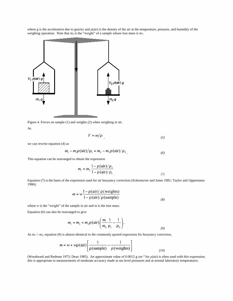
where g is the acceleration due to gravity and ρ(air) is the density of the air at the temperature, pressure, and humidity of the

weighing operation. Note that m2 is the “weight” of a sample whose true mass is m1.

Figure 4. Forces on sample (1) and weights (2) when weighing in air.

As

, (5)

we can rewrite equation (4) as

. (6)

This equation can be rearranged to obtain the expression

. (7)

Equation (7) is the basis of the expression used for air buoyancy correction (Schoonover and Jones 1981; Taylor and Oppermann

1986):

(8)

where w is the “weight” of the sample in air and m is the true mass.

Equation (6) can also be rearranged to give

(9)

As m1 ≈ m2, equation (9) is almost identical to the commonly quoted expression for buoyancy correction,

(10)

(Woodward and Redman 1973; Dean 1985). An approximate value of 0.0012 g cm–3 for ρ(air) is often used with this expression;

this is appropriate to measurements of moderate accuracy made at sea level pressures and at normal laboratory temperatures.

6. References

Dean, J.A. 1985. Lange’s Handbook of Chemistry. McGraw-Hill Book Company, New York, 1792 pp.

Jones, F.E. 1978. The air density equation and the transfer of the mass unit. J. Res. Natl. Bureau Stand., 83, 419–428.

Schoonover, R.M. and Jones, F.E. 1981. Air buoyancy correction in high-accuracy weighing on analytical balances. Anal.

Chem., 53, 900–902.

Taylor, J.K. and Oppermann, H.V. 1986. Handbook for the quality assurance of metrological measurements. National Bureau of

Standards Handbook, 145.

Woodward, C. and Redman, H.N. 1973. High-precision Titrimetry. The Society for Analytical Chemistry, London, 63 pp.

Appendix B:

Gravimetric calibration of volume contained in volumetric flasks and pipettes using water

Taken directly from SOP 13 (Dickson 2007), with additions from Batista (2006)

1. Scope and field of application

This procedure describes how to calibrate the volume of solution contained by volumetric flasks, pipettes or other container

capable of being filled to a reproducible mark. This is expressed as the volume contained at a standard temperature (usually

20.0°C). This procedure is capable of achieving a reproducibility of better than 0.01% (1 relative standard deviation).

“Eppendorf” type air displacement pipettes are commonly used along with volumetric flasks for the preparation of calibration

solutions. These have precision of 0.1% if used carefully. The accuracy is expected to be about 0.1% of the stated value when

the pipette is new. Their precision and accuracy should be checked on regular basis.

2. Principle

The mass of water contained by the flask at a measured calibration temperature is used to compute the volume of water contained

at that temperature. The volume that would be contained at the standard temperature (20°C) can be calculated by taking account

of the volumetric expansion of the flask. The volume of liquid contained at any desired temperature can be calculated in a

similar fashion.

Warning. This requires that the temperature of the calibration solution is known. Taking solutions directly from a refrigerator

and preparing a standard solution should be avoided for this reason. Similarly, pipetting cold solution in an air displacement

pipette can cause an increase in the volume by 5% if a pipette calibrated at 20°C is used to pipette a solution at 5°C. Once in the

pipette, the cold solution can cause the air above it to contract.

Warning. If using micro pipettes for preparing working solutions in LNSW or ASW, first pre-rinse the pipet-tip at its

maximum setting before use, displaced volume can differ up to 0.5%.

3. Apparatus

Analytical balance capable of weighing the quantity of water contained with a sensitivity of 1 part in 105 while having the

capacity to weigh the water together with the container being calibrated.

Thermometer accurate to ± 0.1°C.

Container large enough to retain more than 10 aliquots dispensed by the pipette being calibrated.

4. Reagents

Deionized water (ultrapure) in equilibrium with the temperature of the laboratory.

5. Procedure for the calibration of volumetric flasks

• Weigh the clean, dry, empty container together with the associated closure.

• Fill the container being calibrated to the mark with deionized water, allowing the temperature of the container and contained

water to reach an equilibrium value. Note this temperature.

• Close the container and reweigh it.

6. Calculation and expression of results

6.1 Volume of the water contained at the calibration temperature

Compute the weight of the water contained from the difference between weights of the filled and empty container:

. (11)

Compute the mass of water contained, correcting for air buoyancy (see Appendix A):

(12)

The volume contained at the noted temperature (t) is

(13)

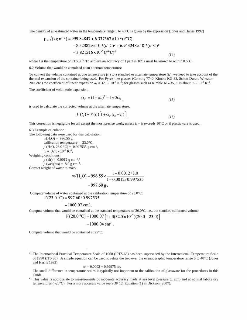
The density of air-saturated water in the temperature range 5 to 40°C is given by the expression (Jones and Harris 1992)

(14)

where t is the temperature on ITS 903. To achieve an accuracy of 1 part in 104, t must be known to within 0.5°C.

6.2 Volume that would be contained at an alternate temperature

To convert the volume contained at one temperature (t1) to a standard or alternate temperature (t2), we need to take account of the

thermal expansion of the container being used. For Pyrex-like glasses (Corning 7740, Kimble KG-33, Schott Duran, Wheaton

200, etc.) the coefficient of linear expansion αl is 32.5 10–7 K–1; for glasses such as Kimble KG-35, αl is about 55 10–7 K–1.

The coefficient of volumetric expansion,

, (15)

is used to calculate the corrected volume at the alternate temperature,

. (16)

This correction is negligible for all except the most precise work; unless t2 – t1 exceeds 10°C or if plasticware is used.

6.3 Example calculation

The following data were used for this calculation:

w(H2O) = 996.55 g,

calibration temperature = 23.0°C,

ρ (H2O, 23.0 °C) = 0.997535 g cm–3,

al = 32.5 10–7 K–1,

Weighing conditions:

ρ (air) = 0.0012 g cm–3,4

ρ (weights) = 8.0 g cm–3.

Correct weight of water to mass:

Compute volume of water contained at the calibration temperature of 23.0°C:

Compute volume that would be contained at the standard temperature of 20.0°C, i.e., the standard calibrated volume:

Compute volume that would be contained at 25°C.

3 The International Practical Temperature Scale of 1968 (IPTS 68) has been superseded by the International Temperature Scale

of 1990 (ITS 90). A simple equation can be used to relate the two over the oceanographic temperature range 0 to 40°C (Jones

and Harris 1992):

t90 = 0.0002 + 0.99975 t68.

The small difference in temperature scales is typically not important to the calibration of glassware for the procedures in this

Guide. 4 This value is appropriate to measurements of moderate accuracy made at sea level pressure (1 atm) and at normal laboratory

temperatures (~20°C). For a more accurate value see SOP 12, Equation (1) in Dickson (2007).

7. Calibration of micro-liter pipettes (Batista 2006)

Weigh the clean dry empty container.

Dispense 10 aliquots of deionized water, recording the weight of each aliquot.

Correct the weight of each aliquot for air buoyancy (see Appendix A).

Calculate the precision achieved, and record the precision and accuracy of the pipette.

8. References

Jones, F.E. and Harris, G.L. 1992. ITS-90 density of water formulation for volumetric standards calibration. J. Res. Natl. Inst.

Stand. Technol., 97, 335–340.

Batista, E., Pinto, L., Filipe, E., and van der Veen, A.M.H. 2006. Calibration of micropipettes: Test methods and uncertainty

analysis. Measurement, 40, 338-342.

Appendix C:

Establishing the linearity of standard calibrations

1. Scope and field of application

If insufficient attention is paid to determining the correct calibration fit to auto-analyzer data, errors of several percent can be

generated. The tests suggested here should be carried out whenever a method is set up or modified, in order to establish whether

a linear or quadratic equation gives the better slope fit to the data. It is particularly important to carry out such tests when

analyzing sample concentrations that are higher than the normal concentration range. Some laboratories have run such tests on a

regular basis during cruises to control the behavior of their system as, particularly when working in high concentration ranges

close to end of the linear range of a method, changes such as a contaminated reagent could shift the output into a non-linear

range.

2. Principle

Non-linearity in the output from an auto-analyzer can come from two sources:

(1) True non-Beer’s Law non-linearity, i.e. when the absorbance of a reacted solution exceeds that for which the

particular method is linear. (In this case, the method should become linear if the reaction mixture is diluted.)

(2) A non-linear output related to the linearization performed by the electronics of the detector.

(In this case the method will not become linear if the reaction mixture is diluted.)

The linearity of a method can be tested by running an appropriate number of standard solutions over the concentration range of

interest and then examining the spread of residual differences between the data, and the best fit linear and quadratic calibration

equations when fitted to that data.

The degree of likely error can then be estimated at the mid-point of the calibration range; ideally this offset should be <0.5%.

3. Requirements

• An auto-analyzer system

• System software set to provide raw data output for peak heights

• Ten standard solutions

• Spreadsheet or statistical software to calculate best fit and residuals

4. Method

1. Set up the auto-analyzer to run the method of interest over the required concentration range.

2. Load the system table (and sample tray) with an appropriate number of standards at the start of the run for the particular

peak height measurement software to work. Load the system with the ten standards. Ensure that each sample is

measured sufficient times to assess the noise of the run, and to take into account variations resulting from peak height

carryover. For ten samples numbered 0 to 9 the order might be 0123456789 9876543210 9876543210 0123456789.

3. Run the samples and download the peak heights for the ten standards at the end of the run.

4. Load the results into Excel or similar software.

5. Plot sample concentration against peak height.

6. Calculate the best fit for both linear and quadratic equations.

7. Calculate the residual difference between the observed and the best fit data points.

8. Plot the residual values against the concentration of the standards. For a good fit, the residuals should vary around zero

with a spread similar to the precision of the method.

5. Example results

Table 3: Example data for linearity check

Std conc Peak height Linear fit Quadratic fit

analyzer data Calculated residuals

0 0 0.0 0.0

1 100 2.2 -1.2

2 200 4.4 -1.4

3 300 6.6 -0.4

4 400 8.7 1.8

5 495 5.9 0.0

6 590 3.1 -0.6

7 685 0.3 -0.1

8 780 -2.5 1.5

9 870 -10.3 -0.8

0 0 0.0 0.0

1 102 4.2 0.8

2 202 6.4 0.6

3 303 9.6 2.6

4 404 12.7 5.8

5 500 10.9 5.0

6 596 9.1 5.4

7 691 6.3 5.9

8 785 2.5 6.5

9 876 -4.3 5.2

0 0 0.0 0.0

1 98 0.2 -3.2

2 198 2.4 -3.4

3 297 3.6 -3.4

4 396 4.7 -2.2

5 490 0.9 -5.0

6 584 -2.9 -6.6

7 679 -5.7 -6.1

8 775 -7.5 -3.5

9 864 -16.3 -6.8

0 0 0.0 0.0

1 101 3.2 -0.2

2 199 3.4 -2.4

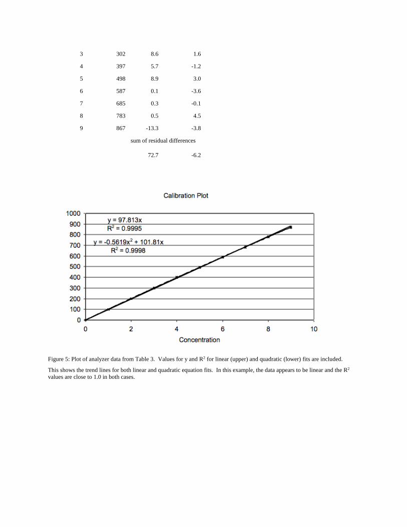
3 302 8.6 1.6

4 397 5.7 -1.2

5 498 8.9 3.0

6 587 0.1 -3.6

7 685 0.3 -0.1

8 783 0.5 4.5

9 867 -13.3 -3.8

sum of residual differences

72.7 -6.2

Figure 5: Plot of analyzer data from Table 3. Values for y and R2 for linear (upper) and quadratic (lower) fits are included.

This shows the trend lines for both linear and quadratic equation fits. In this example, the data appears to be linear and the R2

values are close to 1.0 in both cases.

Figure 6: Plot of the residual difference between the measured values at each standard concentration and the best fit value,

calculated from equations for a linear and a quadratic fit to the data.

A quadratic fit is then applied to both the linear and quadratic sets of residual data.

6. Discussion

The data in Table 3 shows a method that gives a linear response up to the mid-point of the concentration range over which it is

being applied. When both linear and quadratic equations are fitted to the data (Figure 5), relatively high R2 values of 0.9995 and

0.9998, respectively, are returned, and the method appears to be close to linear.

Plotting the residual values between the observed data and the best fit value of the peak height gives a magnified view of the

differences (Figure 6). Clearly, when a linear fit forced through the origin is applied to the data, the values at intermediate

concentrations are overestimated, but underestimated at high concentrations. The sum of the residuals is 73 in this case. Less

bias is shown in the residuals estimated with the quadratic equation; the data is scattered around zero with the sum of the

residuals also close to zero (-6).

Fitting a quadratic equation to the plotted residuals in Figure 6 suggests that the estimate using a linear fit would be 0.7 % high at

mid concentrations and 1.0% low at high concentrations.

7. Conclusions

Before samples are analyzed using a specific method, the linearity of the output for all concentrations should be checked. This is

best done by looking at the residual differences between the observed concentration of standard solutions, and the value obtained

when applying the calibration equation to the peaks of the standard solutions. The most appropriate equation (linear or quadratic)

for calibrating the data can then be selected. A linear slope-only fit can be used if the concentrations of the matrix used to make

the standards is unknown and the standards are all additions to the matrix, as is the case with low nutrient seawater.

Note: If the quadratic equation gives a better fit, the method can then be adjusted to run with a greater degree of dilution to see if

the results become more linear. This will identify if the non-linearity is due to an absorbance which is beyond the Beer’s Law

limit of the method, or due to an inherent problem with the linearity of output from the auto-analyzer’s detector.

Appendix D:

Low-level (nanomolar) nutrients

Different analytical techniques are required to measure nutrient concentrations at the nanomolar level that are typically found in

oligotrophic waters. These nanomolar techniques either use the standard colorimetric analytical techniques but have a more

sensitive detection flow cell like liquid waveguide capillary cells (LWCC), or use different technologies to analyze the nanomolar

concentrations of the nutrients.

The limits of detection for standard autoanalytical techniques is typically 20 nM for phosphate, and nitrate and 10 nM for nitrite.

Although the modern autoanalyser outputs generate data to 5 decimal points, this does not reflect the sensitivity of the instrument

and it is not possible to achieve a limit of detection better than 20 nM on a standard autoanalyzer. Therefore, there are a number

of published methods using liquid waveguides as the detection flowcells, and also other published methodologies, that provide

the means to achieve nutrient values below 20 nM.

Comparison of phosphate concentrations in the ultra-oligotrophic eastern Mediterranean using a conventional CFA system versus

a LWCC revealed that results were comparable between 20 and 100 nM. However, I is seen that the results are more accurate

below 50nM from a LWCC analyser, and certainly below 20 nM, results from the CFA system were deemed unreliable.

Sampling and Storage:

It is imperative that sampling of low nutrient concentration seawater is carried out in as clean conditions as possible.

Samples should be collected in clean, either new or ‘aged’ HDPE sample bottles that are cleaned with 10% HCl and rinsed with

Ultrapure fresh water. Bottles should be stored dry between cruises. In order to avoid the build-up of microbial films whilst at sea

it is recommended to add a small spray of 10% HCl to the bottles between sampling CTD’s. Bottles should be rinsed with

Ultrapure water before sample collection.

To prevent contamination during sample collection, nutrient free gloves should be worn and sampling with bare hands should be

avoided. Vinyl powder-free gloves are currently recommended and coloured nitrile or neoprene gloves should be avoided due to

significant risk of contamination. .

Collection of samples for nanomolar nutrient analysis should occur immediately after collection of samples for oxygen and trace

gases, especially if samples are to be analysed for nanomolar ammonium. Persons sampling before seawater is collected for

nanomolar nutrients should wear vinyl gloves.

Seawater can be taken directly from the spigot of the Niskin bottle. However, it is possible to contaminate samples from water

running of the outside of the Niskin bottle and CTD frame. For consistency, it is recommended to collect samples using an ‘aged’

silicon tube attached to the Niskin bottle spigot. This tube must be clean by soaking in 10% HCL solution between sampling

events and rinsing with Ultrapure water and sample seawter before sample collection. Sample bottles should be rinsed three times

with sample seawater prior to sample collection.

Analysis of seawater samples for nanomolar nutrient concentrations should be carried out as soon as possible after sample

collection. We do not recommend freezing samples for nanomolar nutrient analysis as this can lead to errors of up to 300%.

Atmospheric contamination is an important consideration especially for ammonium. All outside sources like ships emissions, air

vents, and smoking should be avoided if possible. People who have been recently smoking should not be involved in nutrient

sampling because the smoke lingers in the lungs for a number of minutes and this will cause contamination, particularly of

ammonia.

Filtration:

As stated in Section 2.2 above, in general, filtering is not necessary for samples taken in the oligotrophic open ocean, where these

are oligotrophic environments with a very small number of particles in the waters. If sampling is deemed necessary then great

care must be taken not to contaminate the samples during the sample handling and filtering process, all considerations relating to

this are discussed in Section 2.2. It is preferable if filtration is not carried out to avoid any possible contamination.

Analytical Procedures:

a) Nitrate, nitrite and phosphate

A review of the methods used for analysis of nutrients at nanomolar concentrations has been published by Ma et al., 2014.

The chemistry used for nanomolar detection of nutrients is the same for micromolar detection as described above. The most

commonly used sea going analytical detection technique uses the liquid waveguide capillary cells (LWCC), which can vary in

size from 50 cm to 2 m in length. The longer cells are more sensitive but can be more troublesome due to micro bubbles and

analytical noise. Air bubbles need to be removed prior to the flow entering the LWCC but this can often be the source of

problems if small air bubbles are not removed. This is especially problematic for cold water samples that have not reached room

temperature. Cleaning the LWCC is essential and a consistent cleaning protocol is required before and after the analytical run.

The sequential use of Methanol, 10% HCL, and then finally Ultrapure water will keep the LWCC clean.

b) Ammonium

A summary of the more commonly used analytical methods for nanomolar ammonium using colorimetric and fluorimetric

analytical methods are detailed above in Section 5.4.

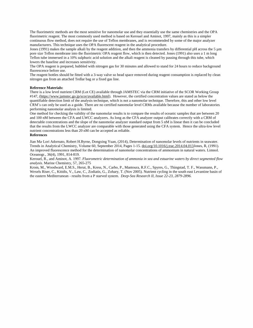
The fluorimetric methods are the most sensitive for nanomolar use and they essentially use the same chemistries and the OPA

fluorimetric reagent. The most commonly used method is based on Kerouel and Aminot, 1997, mainly as this is a simpler

continuous flow method, does not require the use of Teflon membranes, and is recommended by some of the major analyzer

manufacturers. This technique uses the OPA fluorescent reagent in the analytical procedure.

Jones (1991) makes the sample alkali by the reagent addition, and then the ammonia transfers by differential pH across the 5 µm

pore size Teflon membrane into the fluorimetric OPA reagent flow, which is then detected. Jones (1991) also uses a 1 m long

Teflon tube immersed in a 10% sulphuric acid solution and the alkali reagent is cleaned by passing through this tube, which

lowers the baseline and increases sensitivity.

The OPA reagent is prepared, bubbled with nitrogen gas for 30 minutes and allowed to stand for 24 hours to reduce background

fluorescence before use.

The reagent bottles should be fitted with a 3-way valve so head space removed during reagent consumption is replaced by clean

nitrogen gas from an attached Tedlar bag or a fixed gas line.

Reference Materials:

There is a low level nutrient CRM (Lot CE) available through JAMSTEC via the CRM initiative of the SCOR Working Group

#147, (https://www.jamstec.go.jp/scor/available.html). However, the certified concentration values are stated as below the

quantifiable detection limit of the analysis technique, which is not a nanomolar technique. Therefore, this and other low level

CRM’s can only be used as a guide. There are no certified nanomolar level CRMs available because the number of laboratories

performing nanomolar analysis is limited.

One method for checking the validity of the nanomolar results is to compare the results of oceanic samples that are between 20

and 100 nM between the CFA and LWCC analyzers. As long as the CFA analyzer output calibrates correctly with a CRM of

detectable concentrations and the slope of the nanomolar analyzer standard output from 5 nM is linear then it can be concluded

that the results from the LWCC analyzer are comparable with those generated using the CFA system. Hence the ultra-low level

nutrient concentrations less than 20 nM can be accepted as reliable.

References

Jian Ma, Lori Adornato, Robert H.Byrne, Dongxing Yuan, (2014), Determination of nanomolar levels of nutrients in seawater.

Trends in Analytical Chemistry, Volume 60, September 2014, Pages 1-15. doi.org/10.1016/j.trac.2014.04.013Jones, R, (1991).

An improved fluorescence method for the determination of nanomolar concentrations of ammonium in natural waters. Limnol.

Oceanogr., 36(4), 1991, 814-819.

Kerouel, R., and Aminot, A. 1997. Fluorometric determination of ammonia in sea and estuarine waters by direct segmented flow

analysis. Marine Chemistry, 57, 265-275

Krom, M., Woodward, E.M.S., Herut, B., Kress, N., Carbo, P., Mantoura, R.F.C., Spyres, G., Thingstad, T. F., Wassmann, P.,

Wexels Riser, C., Kitidis, V., Law, C., Zodiatis, G., Zohary, T. (Nov 2005). Nutrient cycling in the south east Levantine basin of

the eastern Mediterranean - results from a P starved system. Deep-Sea Research II, Issue 22-23, 2879-2896.

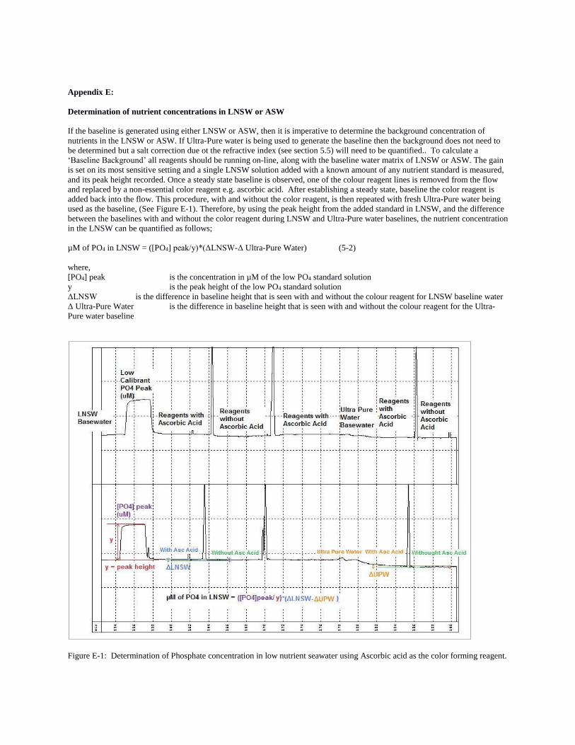
Appendix E:

Determination of nutrient concentrations in LNSW or ASW

If the baseline is generated using either LNSW or ASW, then it is imperative to determine the background concentration of

nutrients in the LNSW or ASW. If Ultra-Pure water is being used to generate the baseline then the background does not need to

be determined but a salt correction due ot the refractive index (see section 5.5) will need to be quantified.. To calculate a

‘Baseline Background’ all reagents should be running on-line, along with the baseline water matrix of LNSW or ASW. The gain

is set on its most sensitive setting and a single LNSW solution added with a known amount of any nutrient standard is measured,

and its peak height recorded. Once a steady state baseline is observed, one of the colour reagent lines is removed from the flow

and replaced by a non-essential color reagent e.g. ascorbic acid. After establishing a steady state, baseline the color reagent is

added back into the flow. This procedure, with and without the color reagent, is then repeated with fresh Ultra-Pure water being

used as the baseline, (See Figure E-1). Therefore, by using the peak height from the added standard in LNSW, and the difference

between the baselines with and without the color reagent during LNSW and Ultra-Pure water baselines, the nutrient concentration

in the LNSW can be quantified as follows;

µM of PO4 in LNSW = ([PO4] peak/y)*(ΔLNSW-Δ Ultra-Pure Water) (5-2)

where,

[PO4] peak is the concentration in µM of the low PO4 standard solution

y is the peak height of the low PO4 standard solution

ΔLNSW is the difference in baseline height that is seen with and without the colour reagent for LNSW baseline water

Δ Ultra-Pure Water is the difference in baseline height that is seen with and without the colour reagent for the Ultra-

Pure water baseline

Figure E-1: Determination of Phosphate concentration in low nutrient seawater using Ascorbic acid as the color forming reagent.

Reference: M. Aoyama, K. Bakker, J. van Ooijen, S. Ossebaar, E.M.S. Woodward (2015). Report from an International Nutrient

Workshop focusing on Phosphate Analysis, 2015, Yang Yang Publisher, Fukushima, Japan. ISBN 978 -4-908583-01-8

Appendix F:

Please note that the analytical methods that follow in Appendix F and G are just examples of the methods used at Scripps and at

JAMSTEC. They not prescriptive as there are many methods available in the literature and supplied by the analytical intrument

suppliers, choice of an analytical method is up to the analysts and individual laboratories themselves.

Detailed methods utilized at SIO/STS/ODF on AA3

NITRATE plus NITRITE ANALYSIS

A modification of the Armstrong et al. (1967) procedure is used for the analysis of nitrate and nitrite. For nitrate analysis, a

seawater sample is passed through a cadmium column where the nitrate is reduced to nitrite. This nitrite is then diazotized with

sulfanilamide and coupled with N-(1-naphthyl)-ethylenediamine to form a red dye. The sample is then passed through a 10mm

flowcell and absorbance measured at 540nm. The procedure is the same for the nitrite analysis but without the cadmium column.

The efficiency of the cadmium column should be determined and tracked over time. Two standards are prepared, one with a high

concentration of nitrate and the other with the same concentration of nitrite. A dilution of secondary standards can be used for

this purpose. The difference in these values gives the column efficiency. If the column efficiency is lower than 95%, the

cadmium column should be reconditioned or replaced.

REAGENTS

Sulfanilamide

Dissolve 10g sulfanilamide in 1.2N HCl and bring to 1 L volume. Add 2 drops of 40% surfynol 465/485 surfactant.

Store at room temperature in a dark poly bottle.

Note: 40% Surfynol 465/485 is 20% 465, plus 20% 485 in DIW.

N-(1-Naphthyl)-ethylenediamine dihydrochloride (N-1-N)

Dissolve 1g N-1-N in DIW, bring to 1 L volume. Add 2 drops 40% surfynol 465/485 surfactant.

Store at room temperature in a dark poly bottle. Discard if the solution turns dark reddish brown.

Imidazole Buffer

Dissolve 13.6g imidazole in ~3.8 L DIW. Stir for at least 30 minutes to completely dissolve. Add 60 ml of CuSO4 + NH4Cl mix

(see below). Add 4 drops 40% Surfynol 465/485 surfactant. Let this sit overnight before proceeding.

Using a calibrated pH meter, adjust to a pH of 7.83-7.85 with 10% (1.2N) HCl (about 20-30 mL of acid, depending on exact

strength). Bring the final solution to 4 L with DIW.

Store at room temperature.

NH4Cl + CuSO4 mix:

Dissolve 2g cupric sulfate in DIW, bring to 100 mL volume (2%)

Dissolve 250g ammonium chloride in DIW, bring to l liter volume.

Add 5ml of 2% CuSO4 solution to this NH4Cl stock. This should last many months.

Nitrate Standard:

In a 1 L calibrated volumetric "A" flask, dissolve ~1.5xxgm of high purity dried KNO3 in DIW to make a 1 L final volume

solution. Record the temperature of the final solution. Calculate the concentration of this primary nitrate standard using the

volumetric flask volume, temperature and exact weight of powder.

Dilute secondary and working standards as necessary.

Nitrite Standard:

In a 1 L calibrated volumetric "A" flask, dissolve ~0.34xxgm of high purity dried NaNO2 in DIW to make a 1 liter final volume

solution. Record the temperature of the final solution. Calculate concentration of this primary standard.

Dilute secondary standard as. Prepare secondary nitrite std daily.

PREPARATION OF PACKED CADMIUM COLUMNS

Cadmium columns are typically prepared on land and shipped ready for use at sea. They can be stored stored in a HDPE

container filled with 50% buffer solution. Before using, the column should be primed (see instructions below). As the columns

wear, they should be topped off with the loose, processed cadmium also stored in the HDPE container. Remember that cadmium

is a toxic substance and it should not be exposed to air once it is processed.

Items needed for Preparation of cadmium column:

Cadmium granules Glass beaker

Buffer Glass stir rod

0.2 M Nitric Acid (N~15.8) 2 % CuSO4

1.2 N (10%) HCl

Processing the cadmium:

Use cadmium granules of approximately 2mm in size. Consolidate all of the cadmium in an oversized glass. Rinse glass column

tubes and end caps with 10% HCl and then DIW. Rinse the cadmium granules with DIW approximately ~ 10 times. Rinses

should be collected as hazardous waste. Stir vigorously between rinses. The rinse water may become cloudy. Then rinse the

cadmium with 1.2N HCl, stir with a stirring rod for a few minutes, and decant the excess. Do this at least twice and until the

solution is clear and the cadmium is shiny. Rinse with ultrapure water 5 to 10 times, being careful to completely rinse all traces

of the HCl. Rinse the cadmium granuals 0.2N nitric acid (~1% solution). This pits the surface of the cadmium to increase the

surface area and may make the solution a bit cloudy. Alternatively pit the surface of the cadmium by using a more concentrated

HCl solution. Do NOT let this solution sit. Rinse with ultrapure water a few times, being sure to rinse away all of the nitric acid.

Rinse a few times with 1.2N HCl again (until the solution is clear again) to get rid of all traces of the nitric acid, then several

rinses (20) with ultrapure water. Add enough ultrapure water to the cadmium to cover the granules, and then begin adding 2%

CuSO4, a little at a time. From this point on, stir gently to protect the copper coating. Stir with a rod in between each addition,

but do not decant. Keep adding slowly until the solution is still slightly bluish in tone, and becomes cloudy. Add CuSO4 until

the blue ceases to disappear and the cadmium turns blackish with lots of particulates (black colloidal particles - broken off pieces

of cadmium). The cadmium is now treated. Do not let this solution sit. Decant almost all of the solution from the cadmium,

minimizing air exposure. Rinse and decant many times with DIW, stirring gently between the rinses. During this entire

procedure, do not stir too vigorously with the glass rod to avoid breaking up the cadmium granules. To remove the fine particles,

stir the liquid above the cadmium to make them rise to the surface and decant them. Continue rinsing until the rinse water is no

longer cloudy, and the cadmium appears dark, spotty, and grayish. Store the granules with imidazole solution.

Packing the columns:

Use an approximately 12mm glass rod with a 1mm wall and 4mm ID. Soak ~ one inch pieces of floss in DIW to prevent bubbles

and make them easier to work with. Pack the bottom with a small ball of dental floss, being sure that it is not too tight and allows

flow). Attach the bottom nipple with silicone tubing (~ID: 1/8” OD: ¼”). Attach a funnel to the top of the empty column and

secure it to a ring stand. Fill a large (~60 ml) syringe with buffer (50%). Attach the syringe to the bottom of the column with

tubing (ID:1/16”). Make sure the tubing is long enough to tie off when finished. Using the syringe, fill the column with buffer

and load the cadmium through the funnel on the top end being sure not to expose the cadmium to the air. Tap the column with a

pencil to pack the cadmium and fill until there is no dead space. Remove the funnel, and insert a ball of dental floss at the top

end. Cap off with the appropriate nipple and silicon tubing. Cap both ends with tied-off tygon tubing. When packing the

column, avoid loading small particulates by scooping cadmium from the bottom of the beaker (the heavier/larger particles).

TOPPING UP THE COLUMN WITH CADMIUM

It is very important to keep the column full of cadmium to minimize dead space. As samples are run, the cadmium volume will

be reduced (through use and settling). This dead space WILL AFFECT THE DATA. To top off the column, turn the AA on and

the column off. Remove the

tubing cap and the floss from the top of the column. Attach the funnel to the top of the column and fill the funnel with buffer.

With a spatula, transfer prepared column granules to the column on the AA, tap with a pencil and continue filling. Leave enough

head space for the dental floss. Remove the excess buffer with the syringe, remove the funnel, reinsert the dental floss ball, and

reconnect the tubing cap to the top of the column. Turn the column on to flush the cadmium, then prime the column.

PRIMING THE COLUMN

The column needs to be primed whenever it is new, or has been topped off with new granules. If the column is not primed, the

response will not be stable. For a new column, prime by running approximately 200 mL of 50uM NO3 standard through the

system with the column turned on. Flush the column afterward by running imidazole and ultrapure water through the system for

30-45mins. If the column has just been topped off, run 100 mLs of 25 to 50 M standard through the system, then flush with

imidazole.

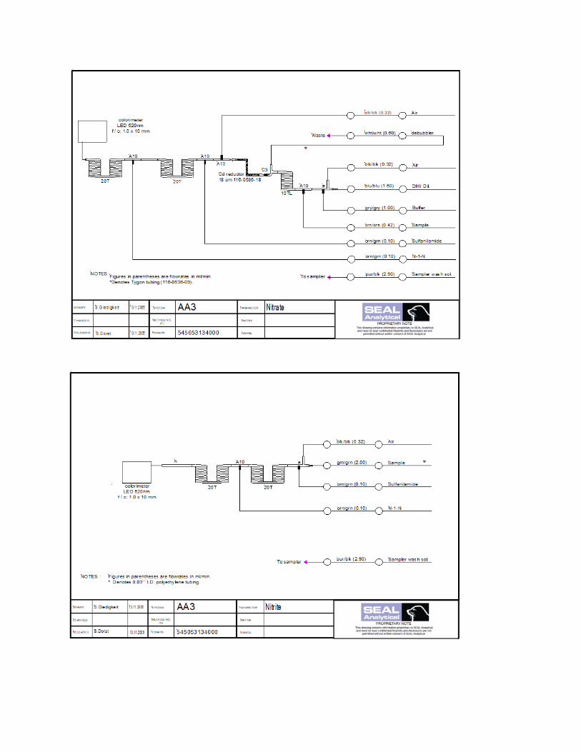
PHOSPHATE ANALYSIS

Ortho-phosphate is analysed using a modification of the Bernhardt and Wilhelms (1967) method. Acidified ammonium

molybdate is added to a seawater sample to produce phosphomolybdic acid, which is then reduced to phosphomolybdous acid (a

blue compound) following the addition of dihydrazine sulfate. The sample is passed through a 10mm flowcell and absorbance

measured at 820nm.

REAGENTS

Ammonium Molybdate

Sulfurica acid sol'n:

Pour 420 ml of ultrapure water into a 2 L Ehrlenmeyer flask or beaker, place this flask or beaker into an ice bath. SLOWLY add

330 ml of concentreated sulfuric acid.

This solution gets VERY HOT!! Cool in the ice bath. Make up as much as necessary in the above proportions.

Dissolve 27g ammonium molybdate in 250 mLof ultrapure. Bring to 1 L volume with the cooled sulfuric acid sol'n. Add 3 drops

of 15% DDS surfactant. Store in a dark poly bottle.

Dihydrazine Sulfate

Dissolve 6.4g dihydazine sulfate in ultrapure water, bring to 1 L volume and refrigerate.

Phosphate Standard:

In a 1 L calibrated volumetric "A" flask, dissolve ~0.81xxgm of dried high purity potassium phosphate in ultrapure water. Record

the temperature. Dilute to the mark with ultrapure water. Calculate the concentration of this primary phosphate standard using

the volumetric flask volume, temperature and exact weight of powder. Dilute a secondary and working standards as necessary.

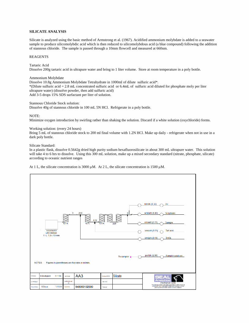
SILICATE ANALYSIS

Silicate is analyzed using the basic method of Armstrong et al. (1967). Acidified ammonium molybdate is added to a seawater

sample to produce silicomolybdic acid which is then reduced to silicomolybdous acid (a blue compound) following the addition

of stannous chloride. The sample is passed through a 10mm flowcell and measured at 660nm.

REAGENTS

Tartaric Acid

Dissolve 200g tartaric acid in ultrapure water and bring to 1 liter volume. Store at room temperature in a poly bottle.

Ammonium Molybdate

Dissolve 10.8g Ammonium Molybdate Tetrahydrate in 1000ml of dilute sulfuric acid*.

*(Dilute sulfuric acid = 2.8 mL concentrated sulfuric acid or 6.4mL of sulfuric acid diluted for phosphate moly per liter

ultrapure water) (dissolve powder, then add sulfuric acid)

Add 3-5 drops 15% SDS surfactant per liter of solution.

Stannous Chloride Stock solution:

Dissolve 40g of stannous chloride in 100 mL 5N HCl. Refrigerate in a poly bottle.

NOTE:

Minimize oxygen introduction by swirling rather than shaking the solution. Discard if a white solution (oxychloride) forms.

Working solution: (every 24 hours)

Bring 5 mL of stannous chloride stock to 200 ml final volume with 1.2N HCl. Make up daily - refrigerate when not in use in a

dark poly bottle.

Silicate Standard:

In a plastic flask, dissolve 0.5642g dried high purity sodium hexafluorosilicate in about 300 mL ultrapure water. This solution

will take 4 to 6 hrs to dissolve. Using this 300 mL solution, make up a mixed secondary standard (nitrate, phosphate, silicate)

according to oceanic nutrient ranges

At 1 L, the silicate concentration is 3000 M. At 2 L, the silicate concentration is 1500 M.

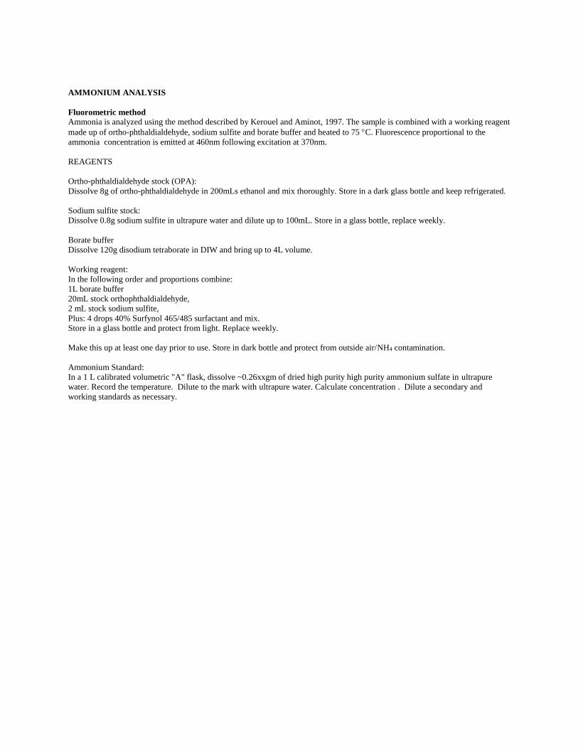
AMMONIUM ANALYSIS

Fluorometric method

Ammonia is analyzed using the method described by Kerouel and Aminot, 1997. The sample is combined with a working reagent

made up of ortho-phthaldialdehyde, sodium sulfite and borate buffer and heated to 75 C. Fluorescence proportional to the

ammonia concentration is emitted at 460nm following excitation at 370nm.

REAGENTS

Ortho-phthaldialdehyde stock (OPA):

Dissolve 8g of ortho-phthaldialdehyde in 200mLs ethanol and mix thoroughly. Store in a dark glass bottle and keep refrigerated.

Sodium sulfite stock:

Dissolve 0.8g sodium sulfite in ultrapure water and dilute up to 100mL. Store in a glass bottle, replace weekly.

Borate buffer

Dissolve 120g disodium tetraborate in DIW and bring up to 4L volume.

Working reagent:

In the following order and proportions combine:

1L borate buffer

20mL stock orthophthaldialdehyde,

2 mL stock sodium sulfite,

Plus: 4 drops 40% Surfynol 465/485 surfactant and mix.

Store in a glass bottle and protect from light. Replace weekly.

Make this up at least one day prior to use. Store in dark bottle and protect from outside air/NH4 contamination.

Ammonium Standard:

In a 1 L calibrated volumetric "A" flask, dissolve ~0.26xxgm of dried high purity high purity ammonium sulfate in ultrapure

water. Record the temperature. Dilute to the mark with ultrapure water. Calculate concentration . Dilute a secondary and

working standards as necessary.

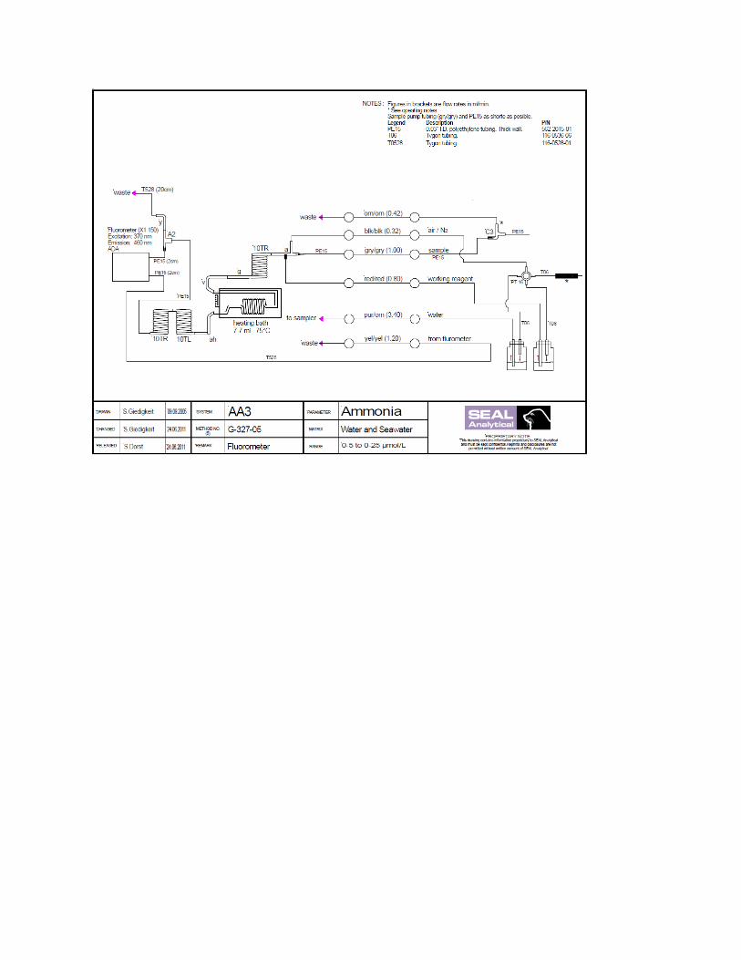
Appendix G:

Detailed methods for QuAAtro 2-HR utilized at JAMSTEC

Nitrate + Nitrite Analysis Nitrate + nitrite and nitrite are analyzed following a modification of the method of Grasshoff (1976). The sample nitrate is

reduced to nitrite in a cadmium tube the inside of which is coated with metallic copper. The sample stream after reduction is

treated with an acidic, sulfanilamide reagent to produce a diazonium ion. N-1-Naphthylethylenediamine Dihydrochloride is

added to the sample stream to produce a red azo dye. With the reduction of the nitrate to nitrite, both nitrate and nitrite react and

are measured together, without reduction, only nitrite reacts. Thus, for the nitrite analysis, no reduction is performed and the

alkaline buffer is not necessary. Nitrate is computed by difference.

REAGENTS for Nitrate: 50 % Triton solution

50 mL TritonTM X-100 provided by Sigma-Aldrich Japan G. K. (CAS No. 9002-93-1) .were mixed with 50 mL Ethanol (99.5 %).

Imidazole (buffer), 0.06 M (0.4 % w/v)

Dissolve 4 g Imidazole (CAS No. 288-32-4), in 1000 mL Ultra-pure water, add 2 mL Hydrogen chloride (CAS No. 7647-01-0).

After mixing, 1 mL 50 % Triton solution is added.

Sulfanilamide, 0.06 M (1 % w/v) in 1.2 M HCl

Dissolve 10 g 4-Aminobenzenesulfonamide (CAS No. 63-74-1), in 900 mL of Ultra-pure water, add 100 mL Hydrogen chloride

(CAS No. 7647-01-0). After mixing, 2 mL 50 % Triton solution is added.

NED, 0.004 M (0.1 % w/v)

Dissolve 1 g N-(1-Naphthalenyl)-1,2-ethanediamine, dihydrochloride (CAS No. 1465-25-4), in 1000 mL of Ultra-pure water and

add 10 mL Hydrogen chloride (CAS No. 7647-01-0). After mixing, 1 mL 50 % Triton solution is added. This reagent is stored in

a dark bottle.

NO3 + NO2 Flow diagram.

REAGENTS for Nitrite: 50 % Triton solution

50 mL TritonTM X-100 provided by Sigma-Aldrich Japan G. K. (CAS No. 9002-93-1) .were mixed with 50 mL Ethanol (99.5 %).

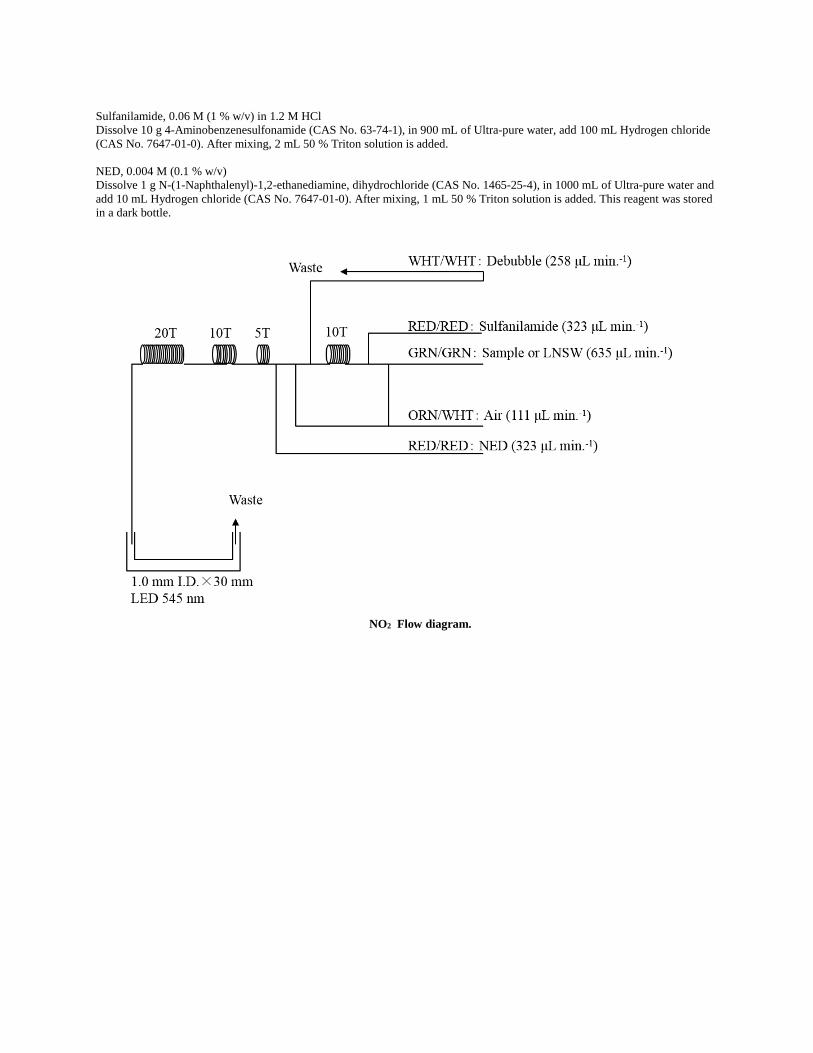
Sulfanilamide, 0.06 M (1 % w/v) in 1.2 M HCl

Dissolve 10 g 4-Aminobenzenesulfonamide (CAS No. 63-74-1), in 900 mL of Ultra-pure water, add 100 mL Hydrogen chloride

(CAS No. 7647-01-0). After mixing, 2 mL 50 % Triton solution is added.

NED, 0.004 M (0.1 % w/v)

Dissolve 1 g N-(1-Naphthalenyl)-1,2-ethanediamine, dihydrochloride (CAS No. 1465-25-4), in 1000 mL of Ultra-pure water and

add 10 mL Hydrogen chloride (CAS No. 7647-01-0). After mixing, 1 mL 50 % Triton solution is added. This reagent was stored

in a dark bottle.

NO2 Flow diagram.

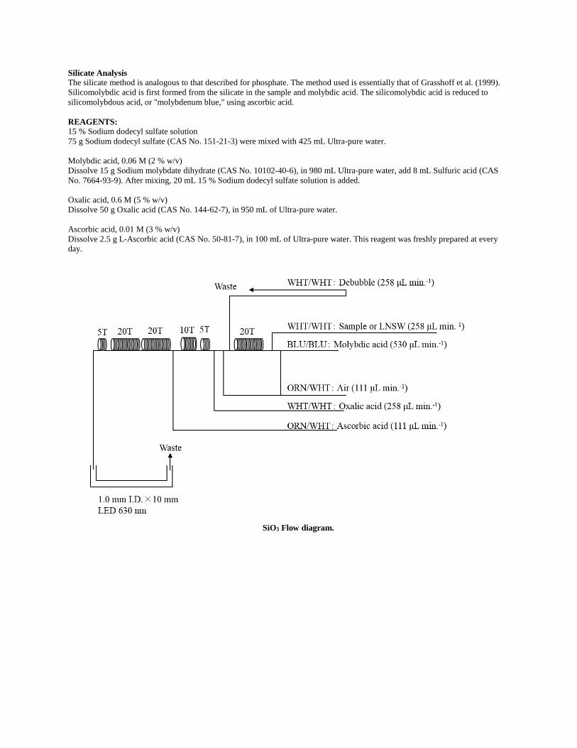
Silicate Analysis The silicate method is analogous to that described for phosphate. The method used is essentially that of Grasshoff et al. (1999).

Silicomolybdic acid is first formed from the silicate in the sample and molybdic acid. The silicomolybdic acid is reduced to

silicomolybdous acid, or "molybdenum blue," using ascorbic acid.

REAGENTS: 15 % Sodium dodecyl sulfate solution

75 g Sodium dodecyl sulfate (CAS No. 151-21-3) were mixed with 425 mL Ultra-pure water.

Molybdic acid, 0.06 M (2 % w/v)

Dissolve 15 g Sodium molybdate dihydrate (CAS No. 10102-40-6), in 980 mL Ultra-pure water, add 8 mL Sulfuric acid (CAS

No. 7664-93-9). After mixing, 20 mL 15 % Sodium dodecyl sulfate solution is added.

Oxalic acid, 0.6 M (5 % w/v)

Dissolve 50 g Oxalic acid (CAS No. 144-62-7), in 950 mL of Ultra-pure water.

Ascorbic acid, 0.01 M (3 % w/v)

Dissolve 2.5 g L-Ascorbic acid (CAS No. 50-81-7), in 100 mL of Ultra-pure water. This reagent was freshly prepared at every

day.

SiO3 Flow diagram.

Phosphate Analysis The phosphate analysis is a modification of the procedure of Murphy and Riley (1962). Molybdic acid is added to the seawater

sample to form phosphomolybdic acid which is in turn reduced to phosphomolybdous acid using L-ascorbic acid as the reductant.

REAGENTS: 15 % Sodium dodecyl sulfate solution

75 g Sodium dodecyl sulfate (CAS No. 151-21-3) were mixed with 425 mL Ultra-pure water.

Stock molybdate solution, 0.03 M (0.8 % w/v)

Dissolve 8 g Sodium molybdate dihydrate (CAS No. 10102-40-6), and 0.17 g Antimony potassium tartrate trihydrate (CAS No.

28300-74-5), in 950 mL of Ultra-pure water and added 50 mL Sulfuric acid (CAS No. 7664-93-9).

PO4 color reagent

Dissolve 1.2 g L-Ascorbic acid (CAS No. 50-81-7), in 150 mL of stock molybdate solution. After mixing, 3 mL 15 % Sodium

dodecyl sulfate solution is added. This reagent was freshly prepared before every measurement.

PO4 Flow diagram.

Ammonia Analysis The ammonia in seawater is mixed with an alkaline containing EDTA, ammonia as gas state is formed from seawater. The

ammonia (gas) is absorbed in sulfuric acid by way of 0.5 µm pore size membrane filter (ADVANTEC PTFE) at the dialyzer

attached to analytical system. The ammonia absorbed in sulfuric acid is determined by coupling with phenol and hypochlorite to

form indophenol blue. Wavelength for ammonia analysis is 630 nm, which is absorbance of indophenol blue.

REAGENTS: 30 % Triton solution

30 mL TritonTM X-100 provided by Sigma-Aldrich Japan G. K. (CAS No. 9002-93-1) .was mixed with 70 mL Ultra-pure water.

EDTA

Dissolve 41 g tetrasodium;2-[2-[bis(carboxylatomethyl)amino]ethyl- (carboxylatomethyl)amino]acetate;tetrahydrate (CAS No.

13235-36-4), and 2 g Boric acid (CAS No. 10043-35-3), in 200 mL of Ultra-pure water. After mixing, 1 mL 30 % Triton solution

is added. This reagent is prepared weekly.

NaOH liquid

Dissolve 5 g Sodium hydroxide (CAS No. 1310-73-2), and 16 g tetrasodium;2-[2-[bis(carboxylatomethyl)amino]ethyl-

(carboxylatomethyl)amino]acetate;tetrahydrate (CAS No. 13235-36-4) in 100 mL of Ultra-pure water. This reagent is prepared

weekly.

Stock nitroprusside

Dissolve 0.25 g Sodium nitroferricyanide dihydrate (CAS No. 13755-38-9) in 100 mL of Ultra-pure water and add 0.2 mL 1M

Sulfuric acid. Stored in a dark bottle and prepared monthly.

Nitroprusside solution

Mix 4 mL stock nitroprusside and 5 mL 1M Sulfuric acid in 500 mL of Ultra-pure water. After mixing, 2 mL 30 % Triton

solution is added. This reagent is stored in a dark bottle and prepared every 2 or 3 days.

Alkaline phenol

Dissolve 10 g Phenol (CAS No. 108-95-2), 5 g Sodium hydroxide (CAS No. 1310-73-2) and 2 g Sodium citrate dihydrate (CAS

No. 6132-04-3), in 200 mL Ultra-pure water. Stored in a dark bottle and prepared weekly.

NaClO solution

Mix 3 mL Sodium hypochlorite (CAS No. 7681-52-9) in 47 mL Ultra-pure water. Stored in a dark bottle and fleshly prepared

before every measurement. This reagent is prepared 0.3 % available chlorine.

NH4 Flow diagram.

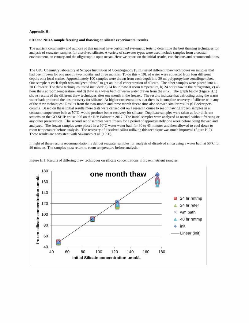
Appendix H:

SIO and NIOZ sample freezing and thawing on silicate experimental results

The nutrient community and authors of this manual have performed systematic tests to determine the best thawing techniques for

analysis of seawater samples for dissolved silicate. A variety of seawater types were used include samples from a coastal

environment, an estuary and the oligotrophic open ocean. Here we report on the initial results, conclusions and recommendations.

The ODF Chemistry laboratory at Scripps Institution of Oceanography (SIO) tested different thaw techniques on samples that

had been frozen for one month, two months and three months. To do this ~ 10L of water were collected from four different

depths on a local cruise. Approximately 100 samples were drawn from each depth into 30 ml polypropylene centrifuge tubes.

One sample at each depth was analyzed “fresh” to get an initial concentration of silicate. The other samples were placed into a -

20 C freezer. The thaw techniques tested included: a) 24 hour thaw at room temperature, b) 24 hour thaw in the refrigerator, c) 48

hour thaw at room temperature, and d) thaw in a water bath of warm water drawn from the sink.. The graph below (Figure H.1)

shows results of the different thaw techniques after one month in the freezer. The results indicate that defrosting using the warm

water bath produced the best recovery for silicate. At higher concentrations that there is incomplete recovery of silicate with any

of the thaw techniques. Results from the two-month and three month freeze time also showed similar results (S Becker pers

comm). Based on these initial results more tests were carried out on a research cruise to see if thawing frozen samples in a

constant temperature bath at 50C would produce better recovery for silicate. Duplicate samples were taken at four different

stations on the GO-SHIP cruise P06 on the R/V Palmer in 2017. The initial samples were analyzed as normal without freezing or

any other preservation. The second set of samples were frozen for a period of approximately one week before being thawed and

analyzed. The frozen samples were placed in a 50C water water bath for 30 to 45 minutes and then allowed to cool down to

room temperature before analysis. The recovery of dissolved silica utilizing this technique was much improved (figure H.2).

These results are consistent with Sakamoto et al. (1990).

In light of these results recommendation is defrost seawater samples for analysis of dissolved silica using a water bath at 50C for

40 minutes. The samples must return to room temperature before analysis.

Figure H.1: Results of differing thaw techniques on silicate concentrations in frozen nutrient samples

40

60

80

100

120

140

160

180

40 60 80 100 120 140 160 180

fro

zen

silic

ate

co

ncen

trati

on

um

ol/L

initial Silicate concentration umol/L

one month thaw

24 hr rmtmp

24 hr refer

wm bath

48 hr rmtmp

init

Linear (init)

Figure H.2:

Figure H1 and H2 need edited. For example, axis need units and units in the correct format. Also, H1 isnt that clear. Is it possible

to plot the different from the initial rather than the absolute value. The differences between defrosting technqiues may be more

obvious then.

y = 0.9917x + 0.0089R² = 1

0

20

40

60

80

100

120

140

0 50 100 150

fro

zen

/50

bat

h t

haw

co

nc

initial concentration

Silicate (umol/L)

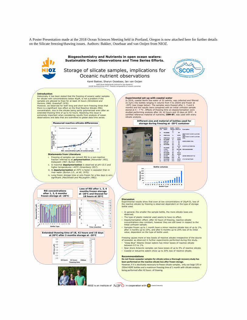
A Poster Presentation made at the 2018 Ocean Sciences Meeting held in Portland, Oregon is now attached here for further details

on the Silicate freezing/thawing issues. Authors: Bakker, Ossebaar and van Ooijen from NIOZ.

Biogeochemistry and Nutrients in open ocean waters: Sustainable Ocean Observations and Time Series Efforts.

Storage of silicate samples, implications for Oceanic nutrient observations

Karel Bakker, Sharyn Ossebaar, Jan van OoijenNIOZ Royal Netherlands Institute for Sea Research;

(SCOR Working Group #147: Towards comparability of oceanic nutrients)

DiscussionExperimental results show that even at low concentrations of 20µM Si, loss of the reactive silicate by freezing is observed dependent on the type of storage bottle used.

• In general, the smaller the sample bottle, the more silicate loses are observed.

• The type of plastic material used seems to have no effect.

• Depolymerisation effect; after 42 hours of thawing, reactive silicate concentrations stay constant, however they are still lower in respect to the initial unfrozen sample.

• Samples frozen up to 1 month have a minor reactive silicate loss of up to 1%, after 3 months up to 10%, and after 6 months up to 25% loss of its initial value, dependent on the type of bottle used.

Freezing causes more or less losses of reactive silicate irrespective of the source of seawater as observed in further experiments performed during this study.

• “Deep Blue” Atlantic Ocean waters has minor losses of reactive silicate between 0.5 to 1%.

• Near shore Antarctic samples can have losses of up to 5% of reactive silicate.

• Coastal or estuarine waters show up to 20% loss of reactive silicate.

Recommendations

Do not freeze seawater samples for silicate unless a thorough recovery study has been performed on the reactive silicate loss after frozen storage. However, if it is absolutely necessary to freeze silicate samples, only use large 125 or 250ml HDPE bottles and a maximum freezing time of 1 month with silicate analysis being performed after 42 hours of thawing.

IntroductionHistorically it has been stated that the freezing of oceanic water samples for silicate with concentrations below 40µM, is not a problem if the samples are allowed to thaw for at least 24 hours (Strickland and Parsons 1968; Grasshoff 1976).However, we observed for both long and short term freezing times that there is a significant loss effect on the final Reactive Silicate (RSi)concentration, due to the silicate being partly polymerized even after an extended thawing time of up to 42 hours. Resolving this issue is extremely important when considering results from analysis of ocean observations and data that are submitted to global data time series.

RSi concentrations after 1, 3, 6 months

frozen storage at -20ºC

Different size and material of bottles used for storage during freezing at -20ºC container

-6

-5

-4

-3

-2

-1

0

1 3 6

RS

ilo

ss (

µM

)

Time (months)

PQA

MOBKJ

NILEC

HFGD

Loss of RSi after 1, 3, 6 months frozen storage

at -20ºC and thawed for 18 hours at 20ºC

Measured reactive silicate differences

-3.0

-2.5

-2.0

-1.5

-1.0

-0.5

0.0

0.5

18 hours 42 hours 10days

RS

ilo

ss (

µM

)

Thawing time

CooledABCDEFGHIJKLMNO

Extended thawing time of 18, 42 hours and 10 days at 20ºC after 3 months storage at -20ºC

Experimental set-up with coastal waterIn 2016, coastal North Sea water of 32 salinity, was collected and filtered (0.7µm) into bottles ranging in volume from 4 to 250ml and frozen at -20ºC (see image below). The samples were thawed after 1, 3 and 6 months and the results were compared with an initial unfrozen sample stored at 4 – 7 ºC . Effects of thawing time on depolymerisation were studied performing analysis after 18, 42 hours and 10 days at 20ºC . A certified reference material of nutrients, CRM-BT, was used with every silicate analysis.

Statements from Literature

i. Freezing of samples can convert RSi to a non-reactive fraction referred to as polymerisation (Alexander 1953, Kobayashi 1967, Burton 1970).

ii. Si maximal depolymerisation is observed at pH>10.5 and higher temperatures >40ºC (Greenberg 1957).

iii. Si depolymerisation at 25ºC is faster in seawater than in river water (Burton.J.D., et All, 1970).

iv. Long frozen storage time or only frozen for a few days is very significant (MacDonald and McLaughlin 1982).

0

10

20

30

40

50

0 20 40 60 80 100 120 140Dif

feren

ce in

RS

i(µ

M)

co

ole

d -

fro

zen

RSi concentration (µM) of cooled sample

14

15

16

17

18

19

20

21

22

Measu

red

RS

i(µ

M)

Bottle Type

1 month

3 month

6 month

Southern Ocean samples