GNR401M Remote Sensing and Image Processing - IIT …avikb/GNR401/DIP/BKM-NRM401-GL3-4... ·...

10/17/2013

1

GNR401M Remote Sensing and Image

ProcessingGuest Instructor: Prof. B. Krishna

Mohan

CSRE, IIT Bombay

[email protected] 5

Guest Lectures 3 – 4 Neighborhood Operations

Sept. 25, 27 2013

9.30 AM – 11.00 AM

Contents of the Lectures

Neighborhood Operations

• Concept of Neighborhood Operations

• Utility of neighborhood in smoothing and edge enhancement

• Image smoothing algorithms

• Gradient operations

• Edge enhancement using gradient operators

IIT Bombay Slide 1

GNR607 GL 3 - 4 B. Krishna Mohan

Sept. 25, 27 2013 GL 3 – 4 Neighborhood Opns

10/17/2013

2

NEIGHBORHOOD OPERATIONS

IIT Bombay Slide 2


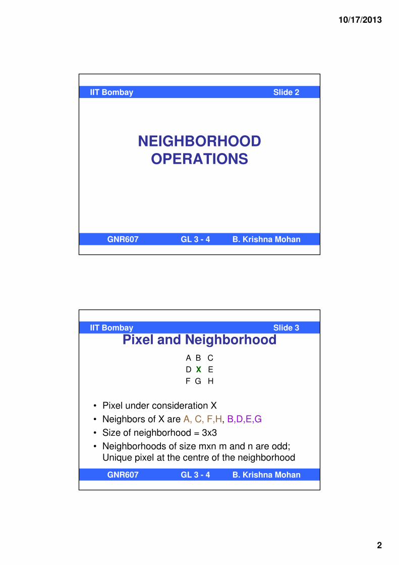
Pixel and Neighborhood

A B C

D X E

F G H

• Pixel under consideration X

• Neighbors of X are A, C, F,H, B,D,E,G

• Size of neighborhood = 3x3

• Neighborhoods of size mxn m and n are odd; Unique pixel at the centre of the neighborhood


IIT Bombay Slide 3

10/17/2013

3

4-neighborhoods

A B C

D X E

F G H

• B,D,E and G are the 4-neighborhood of X

• 4-neighbors are physically closest to X, at

one-unit distance


IIT Bombay Slide 4

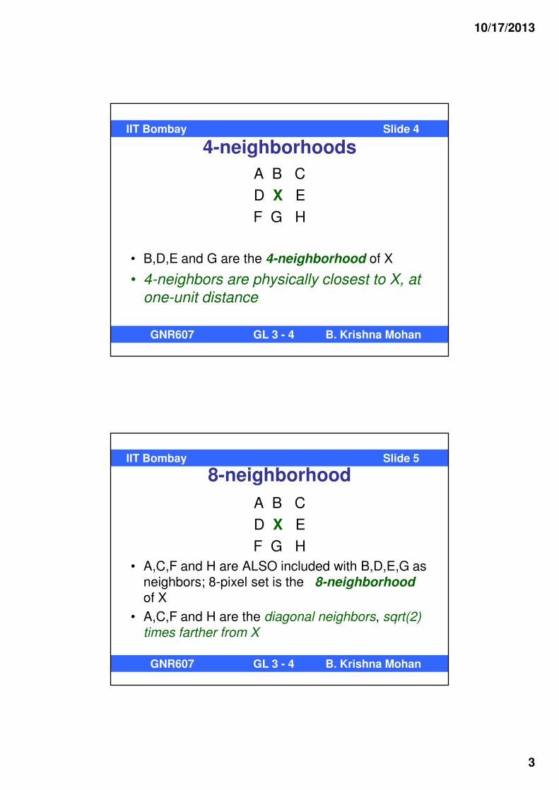
8-neighborhood

A B C

D X E

F G H

• A,C,F and H are ALSO included with B,D,E,G as neighbors; 8-pixel set is the 8-neighborhoodof X

• A,C,F and H are the diagonal neighbors, sqrt(2)

times farther from X


IIT Bombay Slide 5

10/17/2013

4

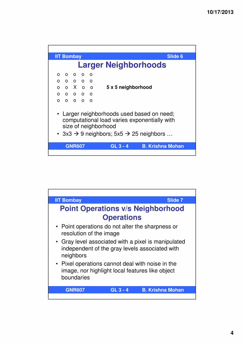
Larger Neighborhoodso o o o o

o o o o o

o o X o o 5 x 5 neighborhood

o o o o o

o o o o o

• Larger neighborhoods used based on need; computational load varies exponentially with size of neighborhood

• 3x3 � 9 neighbors; 5x5 � 25 neighbors …


IIT Bombay Slide 6

Point Operations v/s Neighborhood Operations

• Point operations do not alter the sharpness or resolution of the image

• Gray level associated with a pixel is manipulated independent of the gray levels associated with neighbors

• Pixel operations cannot deal with noise in the image, nor highlight local features like object boundaries


IIT Bombay Slide 7

10/17/2013

5

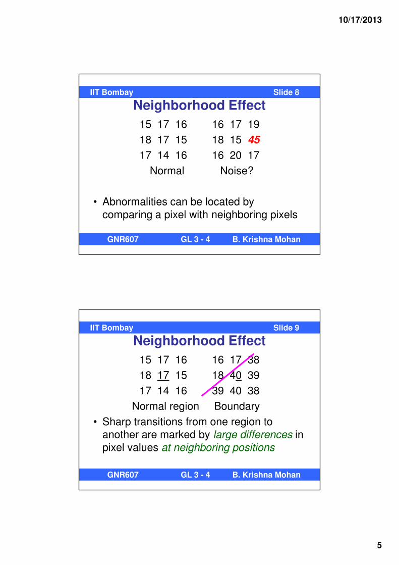
Neighborhood Effect

15 17 16 16 17 19

18 17 15 18 15 45

17 14 16 16 20 17

Normal Noise?

• Abnormalities can be located by

comparing a pixel with neighboring pixels


IIT Bombay Slide 8

Neighborhood Effect

15 17 16 16 17 38

18 17 15 18 40 39

17 14 16 39 40 38

Normal region Boundary

• Sharp transitions from one region to

another are marked by large differences in

pixel values at neighboring positions


IIT Bombay Slide 9

10/17/2013

6


• Results of operations performed on the neighborhood are posted at the location of the central pixel

• The values in the input image are not overwritten, instead the results are stored in an output array or file

• Cannot be computed in real time since the configurations of gray levels in the neighborhood are very large


IIT Bombay Slide 10


• Simple averaging

A B C

D X E

F G H

• g(X) = (1/9)[f(A) + f(B) + f(C) + f(D) + f(X) +

f(E) + f(F) + f(G) + f(H)]

• The output gray level is the average of the gray levels of all the pixels in the 3x3 neighborhood


IIT Bombay Slide 11

10/17/2013

7

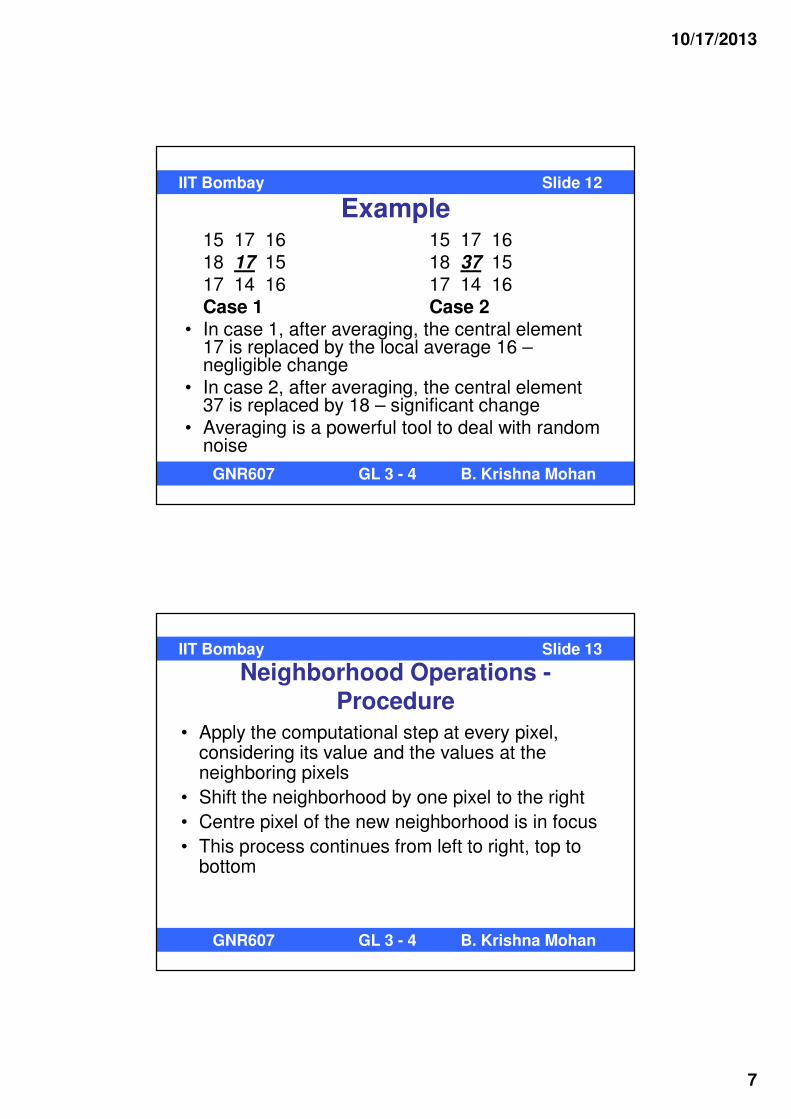
Example15 17 16 15 17 1618 17 15 18 37 1517 14 16 17 14 16Case 1 Case 2

• In case 1, after averaging, the central element 17 is replaced by the local average 16 –negligible change

• In case 2, after averaging, the central element 37 is replaced by 18 – significant change

• Averaging is a powerful tool to deal with random noise


IIT Bombay Slide 12

Neighborhood Operations -Procedure

• Apply the computational step at every pixel, considering its value and the values at the neighboring pixels

• Shift the neighborhood by one pixel to the right

• Centre pixel of the new neighborhood is in focus

• This process continues from left to right, top to bottom


IIT Bombay Slide 13

10/17/2013

8

Image

Processing step


IIT Bombay Slide 14

Mathematical form for averaging

• In general, we can write

g(X) =

where K is the number of neighbors Ai. A5 refers to X, the central pixel for a 3x3 neighborhood.

• It is obvious that all neighbors are given equal weightage during the averaging process

1

( )

| ( ) |

K

i

i

f A

N X

=

∑


IIT Bombay Slide 15

10/17/2013

9

General form for averaging• To assign different weights for different neighbors,

g(X) =

• For simple averaging over a 3x3 neighborhood, wi = (1/9), i=1,2,…,9

• Weights can be altered for 4-neighbors and 8-neighbors. In such a case, wi is not a constant for all values of i.

1

1

( )K

i i

i

K

i

i

w f A

w

=

=

∑

∑


IIT Bombay Slide 16

Averaging as Space Invariant Linear Filtering

• Simple averaging can be represented as a linear space

invariant operation:

k,l= -w, …, 0, …, w

For a 3x3 window, w=1; For 5x5 window, w=2, …

, , ,

,

1

(2 1)(2 1)

l j wk w

i j k l i k j l

k w l j w

k l

g h f

hw w

= +=

− −= = −

=

=+ +

∑ ∑

2-d discrete convolution of h with f; g = f*h


IIT Bombay Slide 17

10/17/2013

10

Concept of Convolution

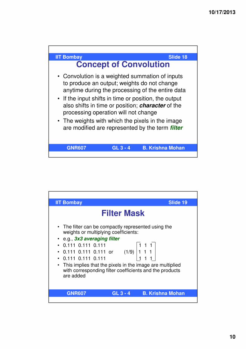
• Convolution is a weighted summation of inputs to produce an output; weights do not change anytime during the processing of the entire data

• If the input shifts in time or position, the output also shifts in time or position; character of the processing operation will not change

• The weights with which the pixels in the image are modified are represented by the term filter


IIT Bombay Slide 18

Filter Mask

• The filter can be compactly represented using the weights or multiplying coefficients:

• e.g., 3x3 averaging filter

• 0.111 0.111 0.111 1 1 1

• 0.111 0.111 0.111 or (1/9) 1 1 1

• 0.111 0.111 0.111 1 1 1

• This implies that the pixels in the image are multiplied with corresponding filter coefficients and the products are added


IIT Bombay Slide 19

10/17/2013

11

Reduced neighborhood influence

0.05 0.15 0.05

0.15 0.20 0.15

0.05 0.15 0.05

• Central pixel is given 20% weight, 4-neighbors 15% weight. Diagonal neighbors given 5% weight.

• Note that the weights are all positive, and sum to unity


IIT Bombay Slide 20

Discrete Convolution

• In general, all the filter coefficients need

not be equal or symmetric

• In that case, the weighted averaging

operation has to be performed using a

discrete convolution procedure

• This is a general operation, assuming that

the process is space invariant.


IIT Bombay Slide 21

10/17/2013

12

Discrete Convolution

• gi,j =

• The filter coefficients are mirror-reflected around the central element, and then the filter is slid on the input image

• The filter moves from top left to bottom right, moving one position at a time

• For each position of the filter, an output value is computed

, ,

w w

k l i k j l

k w l w

h f − −=− =−

∑ ∑


IIT Bombay Slide 22

Image

Filter Mask

IIT Bombay Slide 23


10/17/2013

13

Border Effect

• The computation of the filtering operation

is applicable at those positions of the

image where the filter completely fits

inside.

• At the boundary positions, only part of the

filter fits inside the image. At such

positions, the computation is arbitrarily

defined

IIT Bombay Slide 24


Smoothing• Weighted averaging also referred to as image smoothing

• By smoothing, local differences between pixels are reduced

• Images are often filtered using the same operator throughout, implying shift-invariance

• Most image display adaptors, have hardware convolvers built in to perform 3x3 convolutions in real-time.

• Shift-variant filtering is chosen when local information is to be preserved.

IIT Bombay Slide 25


10/17/2013

14

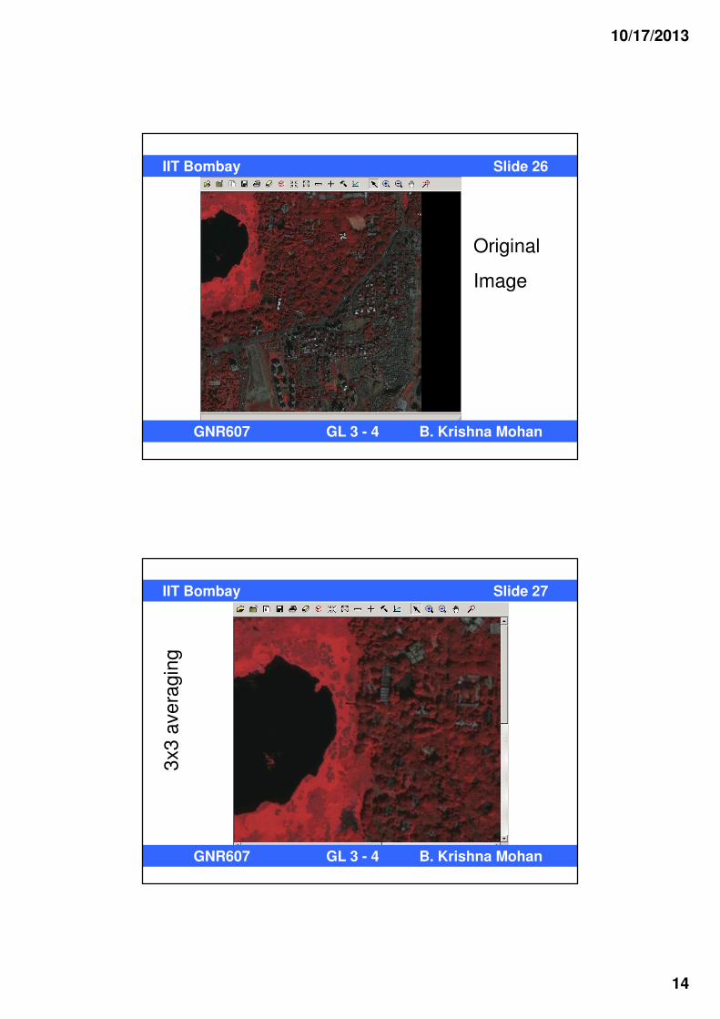
Original

Image

IIT Bombay Slide 26


3x3

ave

rag

ing

IIT Bombay Slide 27


10/17/2013

15

Gaussian smoothing

• Gaussian filter: linear smoothing

• weight matrix

for all

W: one or two σ from center

)(2

12

22

),( σ

cr

kecrw

+−

=

,),( Wcr ∈

∑∈

+−

=

Wcr

cr

e

k

),(

)(2

12

22

1

σ

IIT Bombay Slide 28


Gaussian smoothing• Specify neighborhood size, and σ, get W(r,c) by varying

r,c in the range [–W/2 +W/2]

• Alternatively, find the size of the neighbourhood from 3 σ

limits

• About 99% of the Gaussian distribution is covered within the range mean±3 3 σ

-3 σ ≤ r,c ≤ 3 σ

• If σ = 1, -3 ≤ r,c ≤ 3, size of neighbourhood is 7x7

IIT Bombay Slide 28a


10/17/2013

16

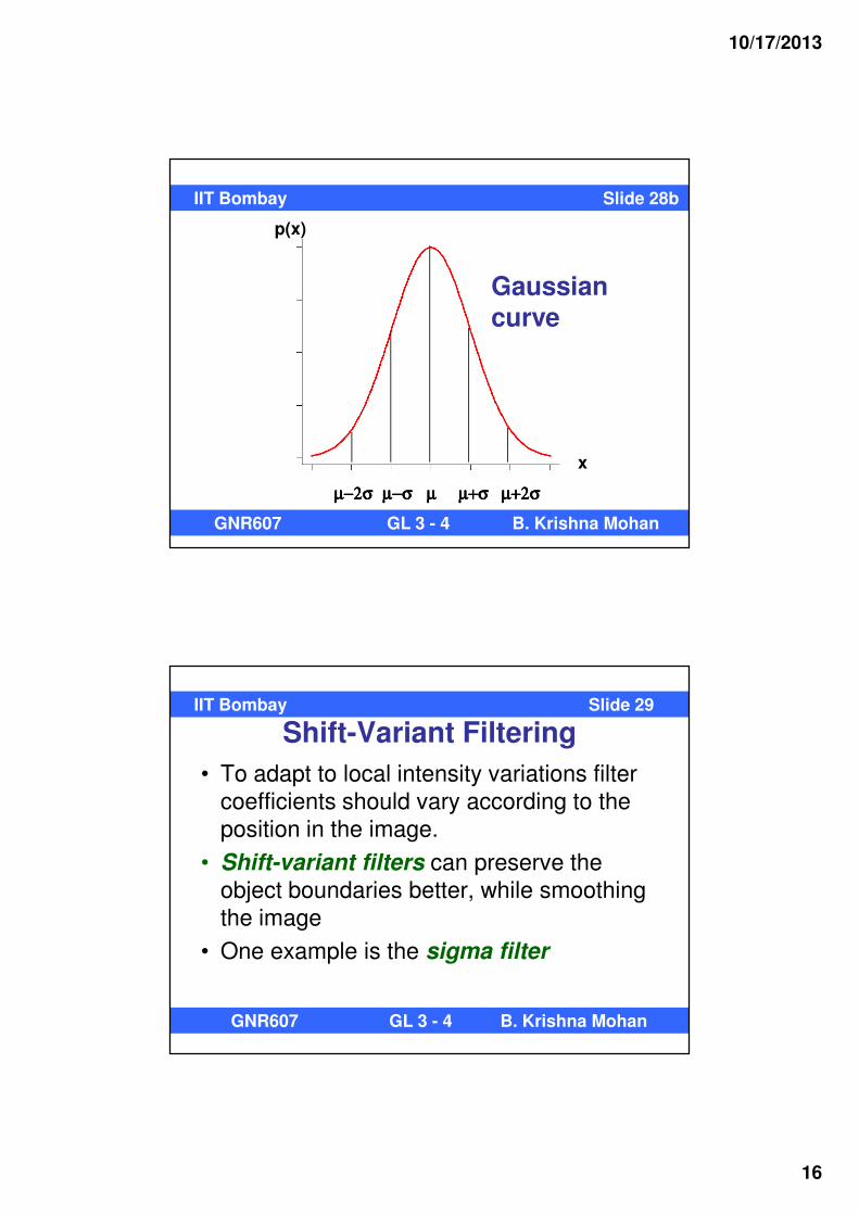
IIT Bombay Slide 28b


x

p(x)

µµµµ−−−−2σ2σ2σ2σ µµµµ−−−−σσσσ µ µ+σ µ+2σµ µ+σ µ+2σµ µ+σ µ+2σµ µ+σ µ+2σ

Gaussian curve

Shift-Variant Filtering

• To adapt to local intensity variations filter

coefficients should vary according to the

position in the image.

• Shift-variant filters can preserve the

object boundaries better, while smoothing

the image

• One example is the sigma filter

IIT Bombay Slide 29


10/17/2013

17

Sigma filter• The underlying principle here is to take the subset of

pixels in the neighborhood whose gray levels lie within c.σof the central pixel gray level

• hi,j,k,l = 0 if |fi-j,k=l – fij | > c.σij ; hi,j,k,l = 1 otherwise

σij is the local standard deviation of the gray levels within

the neighborhood centred at pixel (i,j)

• To save time, one can also use global std. dev.

• c = 1 or 2 depending on the size of neighborhood

, , , , , l j wk i w

i j i j k l i k j l

k i w l j w

g h f= += +

− −= − = −

= ∑ ∑

IIT Bombay Slide 30


Sigma Filter Algorithm• Consider neighborhood size, and value of c

• Find the mean and standard deviation of the pixels within the neighborhood

• Find the neighbors of the central pixel whose gray levels are within c.σ of the central pixel’s gray level

• Compute the average of the pixels meeting the above criterion

• Replace the central pixel’s value by the average

• This cannot be replaced by a convolution since the filter response varies for each position in the image

IIT Bombay Slide 31


10/17/2013

18

Comments on Sigma Filter• Degradation of a smoothed image is due to blurring of

object boundaries

• Here boundaries are better preserved by limiting the smoothing only to a homogeneous subset of pixels in the neighborhood

• The selected subset comprises those pixels that have similar intensities

• Pixels with very different intensities are excluded by making corresponding weights equal to 0



Lee filter

Simple Lee filter

• gij = fmean + k.(fij – fmean)

• k varies between 0 and 1 for smoothing

�k = 0, gij = fmean � simple averaging

�k = 1, gij = fij � no smoothing at all

�k = 2, gij = fij + (fij – fmean)

IIT Bombay Slide 32


10/17/2013

19

Lee filter

IIT Bombay Slide 33


a. Original image

b. Wallis filterc. K=2d. K=3e. K=0.5f. K=0

General form of Lee filter

• The general form of Lee filter is given by

• kij is given by

• Greater noise, smaller kij, hence more smoothing

( )ij mean ij ij meang f k f f= + −

2

2 2 2

ij

ij

mean v ij

kf

σ

σ σ=

+

IIT Bombay Slide 34


10/17/2013

20

Comments on General form of Lee filter

• Noise variance has to be estimated from homogeneous areas

• Unless noise variance is very low, this filter smoothes the image like average filter

• Greater noise, smaller kij, hence more smoothing

2

2 2 2

ij

ij

mean v ij

kf

σ

σ σ=

+



Gradient Inverse Filter

• The gradient inverse filter applies weights to the neighbors in an inverse proportion to their difference to the central pixel (i,j)’s gray level

• Let u(i,j,k,l)=

• Else, u(i,j,k,l) = 2.0

1, ( , ) ( , )

| ( , ) ( , ) |if f i k j l f i j

f i k j l f i j+ + ≠

+ + −

IIT Bombay Slide 35


10/17/2013

21

Gradient Inverse Filter

• The gradient inverse filter is defined by

• hi,j,0,0 = p (=weight for centre pixel), p ≤1

• hi,j,k,l = (1-p)[ui,j,k,l / ] for other pixels∑ i,j,k,lk,l

u

IIT Bombay Slide 36


, , , , , k w l w

i j i j k l i k j l

k w l w

g h f=+ =+

− −=− =−

= ∑ ∑

K-Nearest Neighbor algorithm• Find k-nearest neighbors – k neighbors whose

gray levels are closest to the central pixel in the neighborhood

• Sort the neighbors on the basis of similarity of gray level to the central pixel

• Compute the average of centre pixel and the k nearest neighbors

IIT Bombay Slide 37


10/17/2013

22

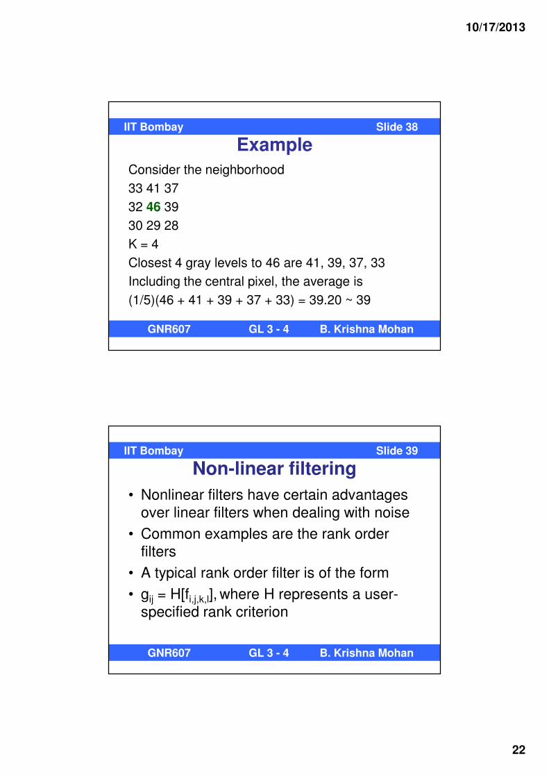
Example

Consider the neighborhood

33 41 37

32 46 39

30 29 28

K = 4

Closest 4 gray levels to 46 are 41, 39, 37, 33

Including the central pixel, the average is

(1/5)(46 + 41 + 39 + 37 + 33) = 39.20 ~ 39

IIT Bombay Slide 38


Non-linear filtering

• Nonlinear filters have certain advantages

over linear filters when dealing with noise

• Common examples are the rank order

filters

• A typical rank order filter is of the form

• gij = H[fi,j,k,l], where H represents a user-

specified rank criterion

IIT Bombay Slide 39


10/17/2013

23

Rank filtering

• Modal filter

• Central pixel is assigned the gray level that occurs most frequently in the neighborhood

• gij = mode {fi-k,j-l | k,l=-w, …, o, …, w}

• e.g., fn = 11 12 14 15 12 16 11 15 15

• Modal filter output = 15

IIT Bombay Slide 40


Median Filter

• Most common non-linear filter for image

smoothing

• Images corrupted by random salt-and-

pepper noise, are effectively smoothed,

without degrading the input image

• gij = median {fi-k,j-l | k,l=-w, …, o, …, w}

IIT Bombay Slide 41


10/17/2013

24

Mean v/s Median filterExample

• 15 17 16 15 17 17

• 18 17 15 157 18 15

• 17 14 16 17 14 16

• Case 1 Case 2• Mean=16 Mean=32

• Median=16 Median=17

• In arithmetic averaging, noise is distributed over the neighbours; in median filtering, the extreme values are pushed to the extremes of the sequence

IIT Bombay Slide 42


Algorithm• Consider the size of the window around the pixel

• Collect all the pixels in the window and sort them in ascending / descending order

• Select the gray level after sorting, according to the rank criterion

• It can easily be verified that median and mode filters are nonlinear, according to the definition of linearity

IIT Bombay Slide 43


10/17/2013

25

Example

Median

filtering

Example here

is over 7x7

neighborhood

IIT Bombay Slide 44


Trimmed Mean Filter

• Trimmed-Mean Operator:

• trimmed-mean: first k and last k gray levels not used

• trimmed-mean: equal weighted average of central N-2k elements

∑−

+=−=

kN

kn

nmeantrimmed xkN

z1

)(2

1

IIT Bombay Slide 45


10/17/2013

26

Some Comments• Shift variant filters can adapt to the image

conditions better

• More computations are involved in shift variant filtering

• Gaussian smoothing has some optimal properties for which it is popular

• Degree of smoothing can be controlled by

varying the width σ of the Gaussian filter

IIT Bombay Slide 46


Comments contd…• Simple averaging type filters fare poorly in

case of signal dependent noise

• Particularly with SAR images noise suppression is challenging

• Noise filtering is performed in case of SAR prior to image formation or after image formation

• Shift variant and nonlinear filters more successful with SAR images

IIT Bombay Slide 47


10/17/2013

27

Comments contd…• An important requirement of image smoothing:

the sharpness in the image should be least affected

• Many comparative studies to evaluate methods

• Estimating noise statistics key to improving quality of data like SAR images

• Additional techniques – based on mathematical morphology

IIT Bombay Slide 48


Edge Enhancement Methods

10/17/2013

28

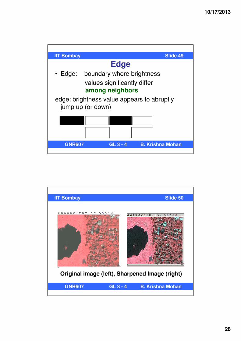
Edge• Edge: boundary where brightness

values significantly differ

among neighbors

edge: brightness value appears to abruptly

jump up (or down)

IIT Bombay Slide 49


IIT Bombay Slide 50


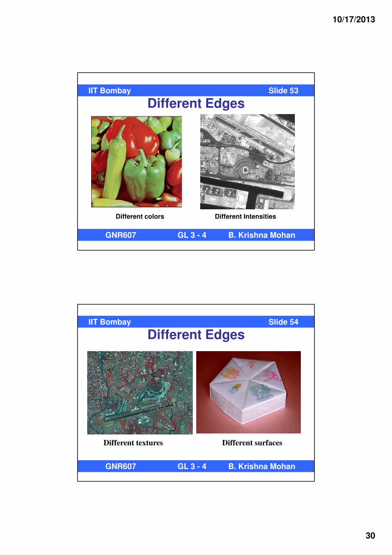
Original image (left), Sharpened Image (right)

10/17/2013

29

Edge Detection

Essential to mark the boundaries of objects

Area, shape, size, perimeter, etc. can be computed from clearly

identified object boundaries

Intensity / color / texture / surface orientation gradient

employed to detect edges

Gradient magnitude denotes the strength of edge

Gradient direction relates to direction of change of intensity /

color

IIT Bombay Slide 51


How is an edge perceived?

• An edge is a set of connected pixels that lie

on the boundary between two regions

• The pixels on an edge are called edge

points

• Gray level / color / texture discontinuity

across an edge causes edge perception

• Position & orientation of edge are key

properties

IIT Bombay Slide 52


10/17/2013

30

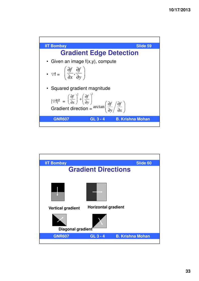
Different Edges

A

Different colors

Different brightness

IIT Bombay Slide 53


Different Intensities

Different Edges

Different textures Different surfaces

IIT Bombay Slide 54


10/17/2013

31

Types Of EdgesGray level profile derivatives

• Step edge:

• Ramp edge:

• Peak edge:

2nd

1st

1st

IIT Bombay Slide 55


Locating an Edge

• Locating an edge is important, since the

shape of an object, its area, perimeter and

other such measurements are possible

only when the boundary is accurately

determined

• Edge is a local feature, marked by sharp

discontinuity in the image property on

either side of it

IIT Bombay Slide 56


10/17/2013

32

Edge• Edge: boundary where brightness

values significantly differ

among neighbors

edge: brightness value appears to abruptly

jump up (or down)

IIT Bombay Slide 57


Principle of Gradient Operator

The interpretation of this operator is that the

intensity gradient is computed in two

perpendicular directions, followed by the

resultant whose magnitude and orientation

are computed by treating the values from

the two masks as two projections of the

edge vector

IIT Bombay Slide 58


10/17/2013

33

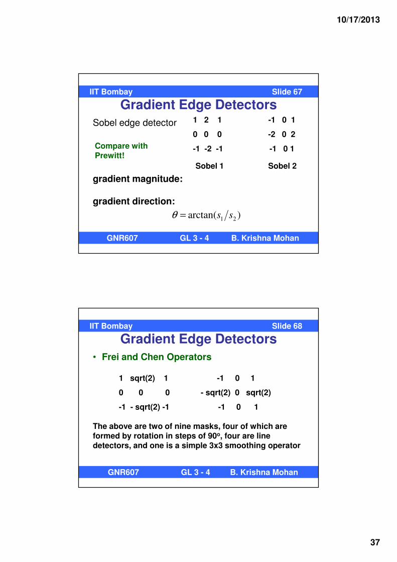
Gradient Edge Detection• Given an image f(x,y), compute

• �f =

• Squared gradient magnitude

|�f|2 =

Gradient direction =

,f f

x y

∂ ∂

∂ ∂

22f f

x y

∂ ∂ +

∂ ∂ arctan

f f

y x

∂ ∂

∂ ∂

IIT Bombay Slide 59


Gradient Directions

Vertical gradient Horizontal gradient

Diagonal gradient

IIT Bombay Slide 60


10/17/2013

34

Gradient Edge Detectors

• As seen, two mutually perpendicular gradient detectors are required to detect edges in an image, since edges may occur in any orientation.

• Using two mutually perpendicular orientations, an edge in any direction can be resolved in terms of these two orthogonal components

IIT Bombay Slide 61


Roberts Operator• Roberts operator: two 2X2 masks to

calculate gradient; Operates on 2x size neighborhood

gradient magnitude: r1 = f(A) – f(D); r2 = f(B) – f(C) r1, r2 gradient outputs from the masks; direction = arctan(r2/r1)

2

2

2

1 rr +

1 0 0 1

0 -1 -1 0

A B

C D

IIT Bombay Slide 62


10/17/2013

35

Gradient Edge Detectors• Prewitt Operator

• gradient magnitude:

• gradient direction: clockwise w.r.t. column axis

• p1, p2 are gradient outputs from the masks

2

2

2

1 ppg +=

)arctan( 21 pp=θ

1 1 1 -1 0 1

0 0 0 -1 0 1

-1 -1 -1 -1 0 1

Prewitt 1 Prewitt 2

IIT Bombay Slide 63



• Prewitt Edge Detector (one part of it)

)()1()(' xfxfxf −+=

)1()()1(' −−=− xfxfxf+

x-1 x x+1

-1 0 1

-1 0 1

-1 0 1 = f (x+1) – f (x -1)

More stable than Roberts, robust to noise in the image, and produces better edges. More time consuming,

IIT Bombay Slide 64


10/17/2013

36

Input image

IIT Bombay Slide 65


Prewitt Operator Output

IIT Bombay Slide 66


10/17/2013

37


Sobel edge detector

)arctan( 21 ss=θ

gradient magnitude:

gradient direction:

1 2 1 -1 0 1

0 0 0 -2 0 2

-1 -2 -1 -1 0 1

Sobel 1 Sobel 2

Compare with Prewitt!

IIT Bombay Slide 67



• Frei and Chen Operators

The above are two of nine masks, four of which are formed by rotation in steps of 90o, four are line detectors, and one is a simple 3x3 smoothing operator

1 sqrt(2) 1 -1 0 1

0 0 0 - sqrt(2) 0 sqrt(2)

-1 - sqrt(2) -1 -1 0 1

IIT Bombay Slide 68


10/17/2013

38

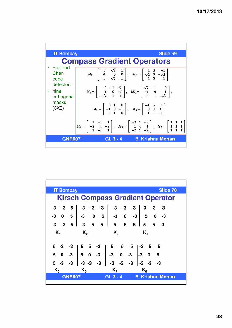
Compass Gradient Operators• Frei and

Chen

edge

detector:

• nine

orthogonal

masks

(3X3)

IIT Bombay Slide 69


Kirsch Compass Gradient Operator

-3 - 3 5 -3 - 3 -3 -3 - 3 -3 -3 -3 -3

-3 0 5 -3 0 5 -3 0 -3 5 0 -3

-3 -3 5 -3 5 5 5 5 5 5 5 -3

K1 K2 K3 K4

5 -3 -3 5 5 -3 5 5 5 -3 5 5

5 0 -3 5 0 -3 -3 0 -3 -3 0 5

5 -3 -3 -3 -3 -3 -3 -3 -3 -3 -3 -3

K5 K6 K7 K8

IIT Bombay Slide 70


10/17/2013

39

Kirsch Gradient Edge Detectors

• Kirsch: set of eight compass template edge masks

gradient magnitude:

gradient direction:

kmax , k = 1,2, ..., 9kg e=

45 arg max keθ = �

IIT Bombay Slide 71


Robinson Gradient Detector

� Robinson: compass template mask set with only ∓0, ∓1, ∓2

Other four masks are mirror reflections of the first fourGradient magnitude and direction same as Kirsch

-1 0 1 -2 -1 0 -1 -2 -1 0 -1 -2

-2 0 2 -1 0 1 0 0 0 1 0 -1

-1 0 1 0 1 2 1 2 1 2 1 0

R1 R2 R3 R4

IIT Bombay Slide 72


10/17/2013

40

Actual Edges

• The edge enhanced images are

thresholded in order to suppress the

interior portions of the image and retain

only the edges

• This helps in identifying the outlines of the

objects of interest

IIT Bombay Slide 73


Prewitt operator output thresholded at 40

IIT Bombay Slide 74


10/17/2013

41

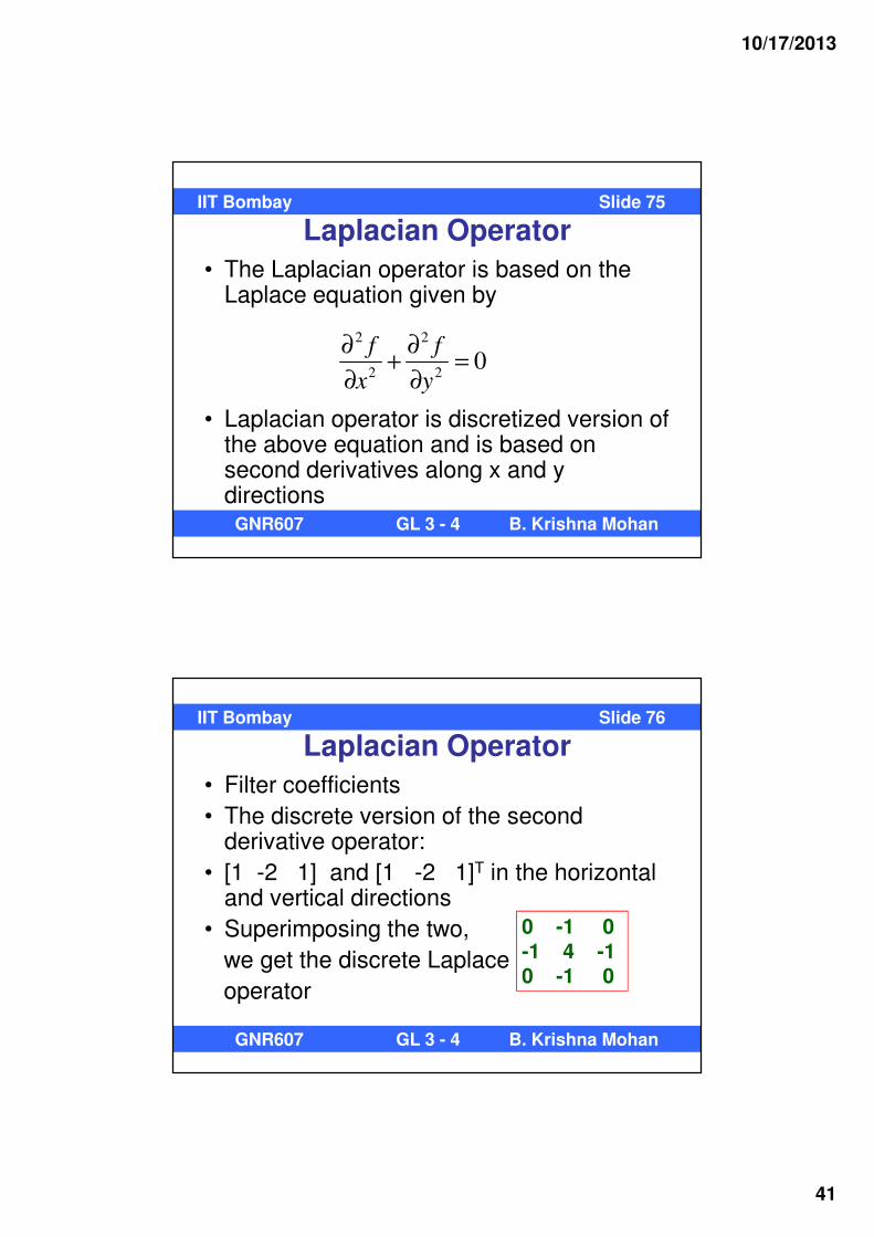
Laplacian Operator

• The Laplacian operator is based on the Laplace equation given by

• Laplacian operator is discretized version of the above equation and is based on second derivatives along x and y directions

2 2

2 20

f f

x y

∂ ∂+ =

∂ ∂

IIT Bombay Slide 75


Laplacian Operator

• Filter coefficients

• The discrete version of the second derivative operator:

• [1 -2 1] and [1 -2 1]T in the horizontal and vertical directions

• Superimposing the two,

we get the discrete Laplace

operator

0 -1 0-1 4 -10 -1 0

IIT Bombay Slide 76


10/17/2013

42

Properties of Laplace Operator

• Isotropic operator – cannot give orientation information

• Any noise in image gets amplified

• Faster since only one filter mask involved

• Smoothing the image first prior to Laplace operator is often needed for reliable edges

IIT Bombay Slide 77


Zero-Crossing Edge Detectors• First derivative maximum: exactly where

second derivative zero crossing• In order to detect edges, we look at pixels

where the intensity gradient is high, or the first derivative magnitude is maximum

• First derivative maximum implies a zero when the second derivative is computed

• Edges are located at those positions where there is a positive value on one side and a negative value on the other side, in other words a zero-crossing

IIT Bombay Slide 78


10/17/2013

43

A step edge, whose first derivative is an impulse, and whose second derivative shows a transition from a positive to a negative

Edge location corresponds to the point where a sign change occurs from positive to negative (or vice versa)

IIT Bombay Slide 79


Zero-Crossing Edge Detectors

• Laplacian of a function I(r,c)

2

2

2

2

2

2

2

22 )(

c

I

r

II

crI

∂

∂+

∂

∂=

∂

∂+

∂

∂=∇

Two commonly used masks for Laplacian operator

IIT Bombay Slide 80


10/17/2013

44

Zero Crossing Edge Detector

• Direct operation on the image using the

Laplacian operator results in a very noisy

result

• Derivative operator amplifies the high

frequency noise

• Preprocess the input image by a

smoothing operator prior to application of

the Laplacian

IIT Bombay Slide 81


Zero Crossing Edge Detector

• The Gaussian shaped smoothing operator

is found to be ideal as a preprocessing

operator

• Therefore the Laplacian operator is

applied on Gaussian smoothed input

image

• ZC(image) = Laplacian [gaussian(image)]

IIT Bombay Slide 82


10/17/2013

45

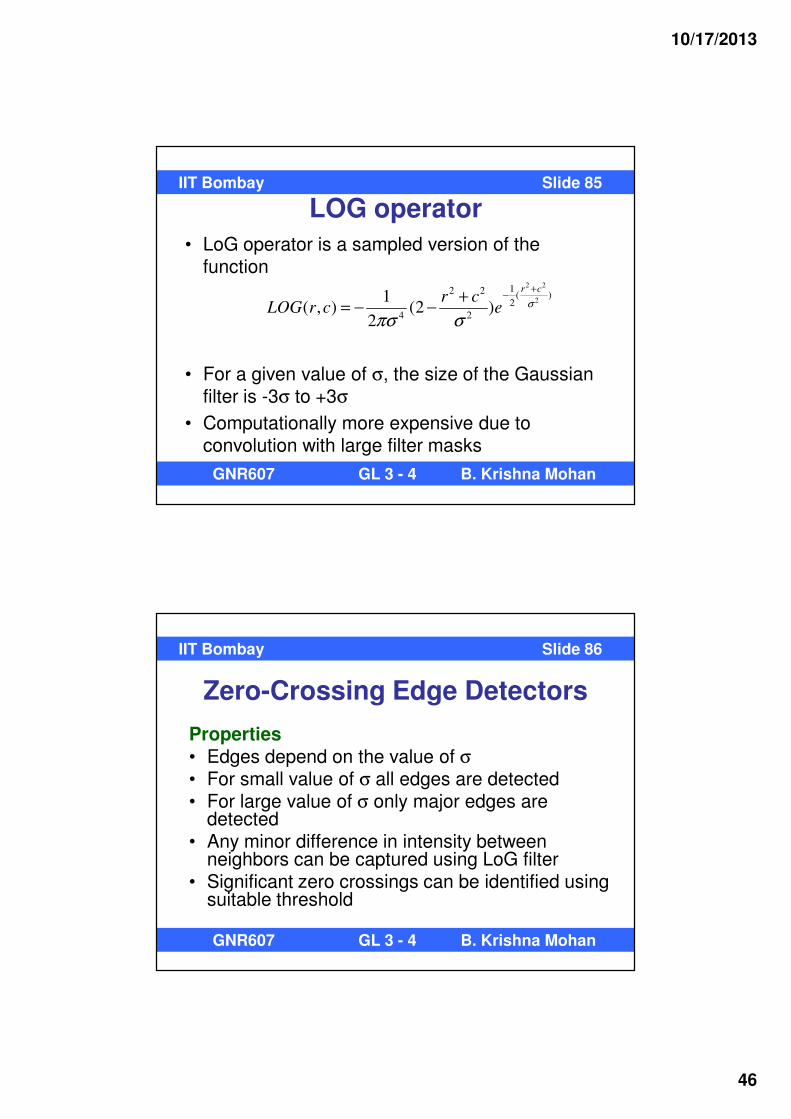
LOG operator

• Both Laplacian operator and Gaussian

operator are linear, and hence can be

combined into one Laplacian of Gaussian

(LoG) operator

• Laplacian[Gaussian(image)] =

[Laplacian(Gaussian)](image)

IIT Bombay Slide 83


LOG operator• Laplacian[Gaussian(image)] =

[Laplacian(Gaussian)](image)

2 2

2

2 2

2

2 2

2

1 2( )2

4 2

1 2( )2

4 2

12 2 ( )2

4 2

1( , ) (1 )

2

1 [ (1 )]

2

1(2 )

2

r c

r c

r c

rLOG r c e

ce

r ce

σ

σ

σ

πσ σ

πσ σ

πσ σ

+−

+−

+−

= − − +

− −

+= − −

Verify!

IIT Bombay Slide 84


10/17/2013

46

LOG operator

• LoG operator is a sampled version of the function

• For a given value of σ, the size of the Gaussian filter is -3σ to +3σ

• Computationally more expensive due to convolution with large filter masks

2 2

2

12 2 ( )2

4 2

1( , ) (2 )

2

r cr c

LOG r c e σ

πσ σ

+−+

= − −

IIT Bombay Slide 85



Properties

• Edges depend on the value of σ• For small value of σ all edges are detected• For large value of σ only major edges are

detected• Any minor difference in intensity between

neighbors can be captured using LoG filter• Significant zero crossings can be identified using

suitable threshold

IIT Bombay Slide 86


10/17/2013

47


• A pixel at (m,n) is declared to have a zero

crossing if

f’’(m,n) > T and f’’(m+δm, n+δn) < -T

OR

f’’(m,n) < -T and f’’(m+δm, n+δn) > T

IIT Bombay Slide 87


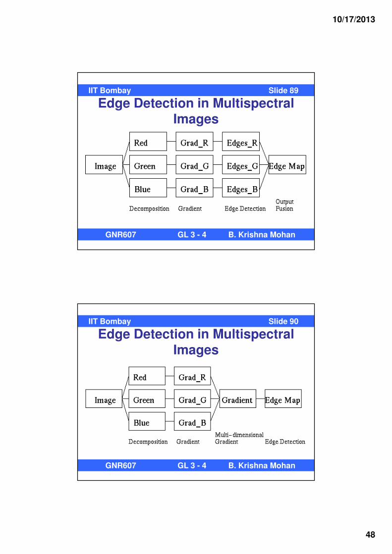
Edge Detection in Multispectral Images

• Simple approaches:

– Compute gradient by taking Euclidean distance

between multispectral vectors of data at adjacent

pixels instead of differences in gray levels

– Find independent gradients for different bands, edges

and combine edges

– Find independent gradients, combine gradients, and

find edge from multiband gradient

IIT Bombay Slide 88


10/17/2013

48


IIT Bombay Slide 89



IIT Bombay Slide 90


10/17/2013

49

Image Sharpening

For example,

• Sharpened image =

Original image + k. gradient magnitude

• Scale factor k can determine whether

gradient magnitude is added as it is or a

fraction of it. The sum may be rescaled to

0-255 to display like an image

IIT Bombay Slide 92


IIT Bombay Slide 93


Original image (left), Sharpened Image (right)

10/17/2013

50

Unsharp Masking

• Sample convolution mask

0 0 0 0 0 0 1 1 1

0 1 0 + 0 1 0 - (1/9) 1 1 1

0 0 0 0 0 0 1 1 1

G = F + | (F – Fmean) |

IIT Bombay Slide 94

NR607 GL 3 - 4 B. Krishna Mohan

IIT Bombay Slide 95

NR607 GL 3 - 4 B. Krishna Mohan

10/17/2013

51

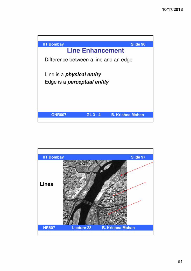
Line Enhancement

Difference between a line and an edge

Line is a physical entity

Edge is a perceptual entity

IIT Bombay Slide 96


IIT Bombay Slide 97

NR607 Lecture 28 B. Krishna Mohan

Lines

10/17/2013

52

Line Enhancement

Detection of a physical line involves

High to low transition � Low to high transition

OR

Low to high transition � High to low transition

IIT Bombay Slide 98


Line Enhancement Masks

• These masks look for positive to negative and negative to positive transitions in vertical/horizontal/diagonal directions

IIT Bombay Slide 99


10/17/2013

53

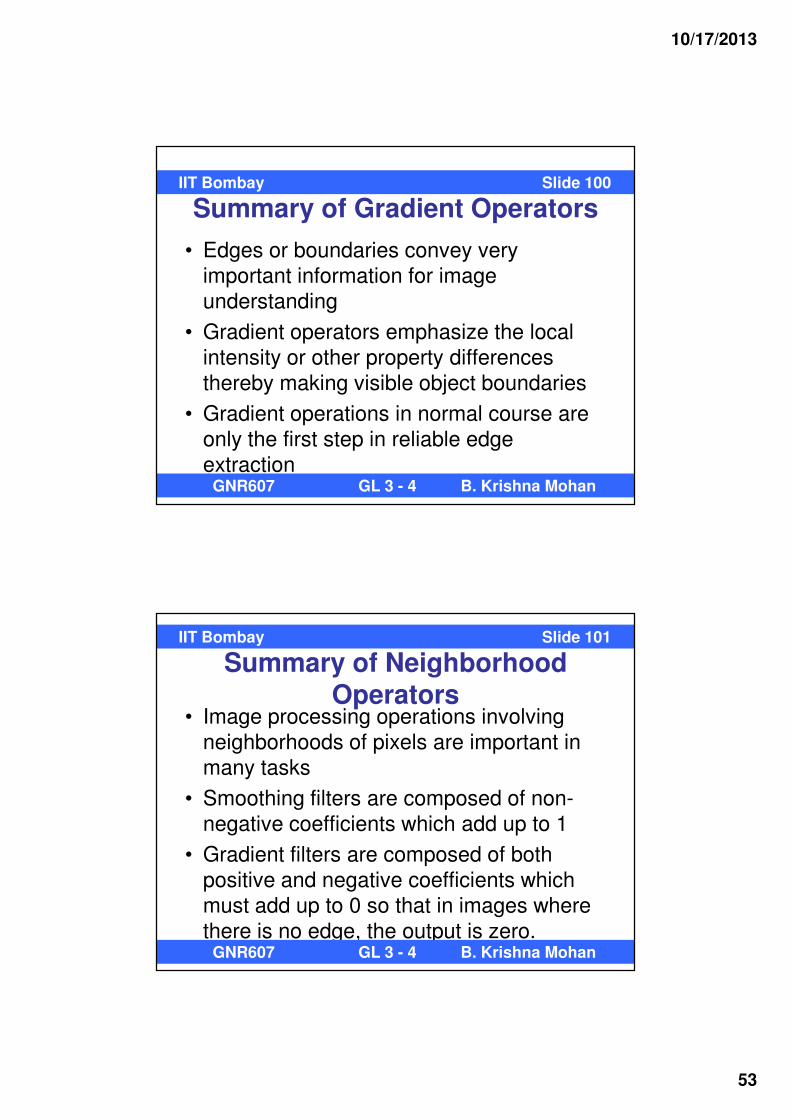
Summary of Gradient Operators

• Edges or boundaries convey very

important information for image

understanding

• Gradient operators emphasize the local

intensity or other property differences

thereby making visible object boundaries

• Gradient operations in normal course are

only the first step in reliable edge

extraction

IIT Bombay Slide 100


Summary of Neighborhood Operators

• Image processing operations involving

neighborhoods of pixels are important in

many tasks

• Smoothing filters are composed of non-

negative coefficients which add up to 1

• Gradient filters are composed of both

positive and negative coefficients which

must add up to 0 so that in images where

there is no edge, the output is zero.



10/17/2013

54

Shape Fitting by Hough Transform



Hough Transform• A method for finding global relationships

between pixels.

Example: We want to find straight lines in an image

• Apply Hough transform to the edge enhanced –thresholded image

• Any curve that can be represented by a parametric equation can be extracted by Hough transform



10/17/2013

55

Line Fitting



EdgesLines fit to the edges

Hough transform ProcedureConsider a set of points xi, yi on a line y = a.x + b; a and

b are parameters (slope and intercept)

All the above points satisfy the equation yi = a.xi + b

Let xi and yi be the parameters; then b = -a.xi + yi

Vary a and find corresponding b. In the “a-b” space, it is a line

For each xi, yi there is a line in the “a-b” space



10/17/2013

56

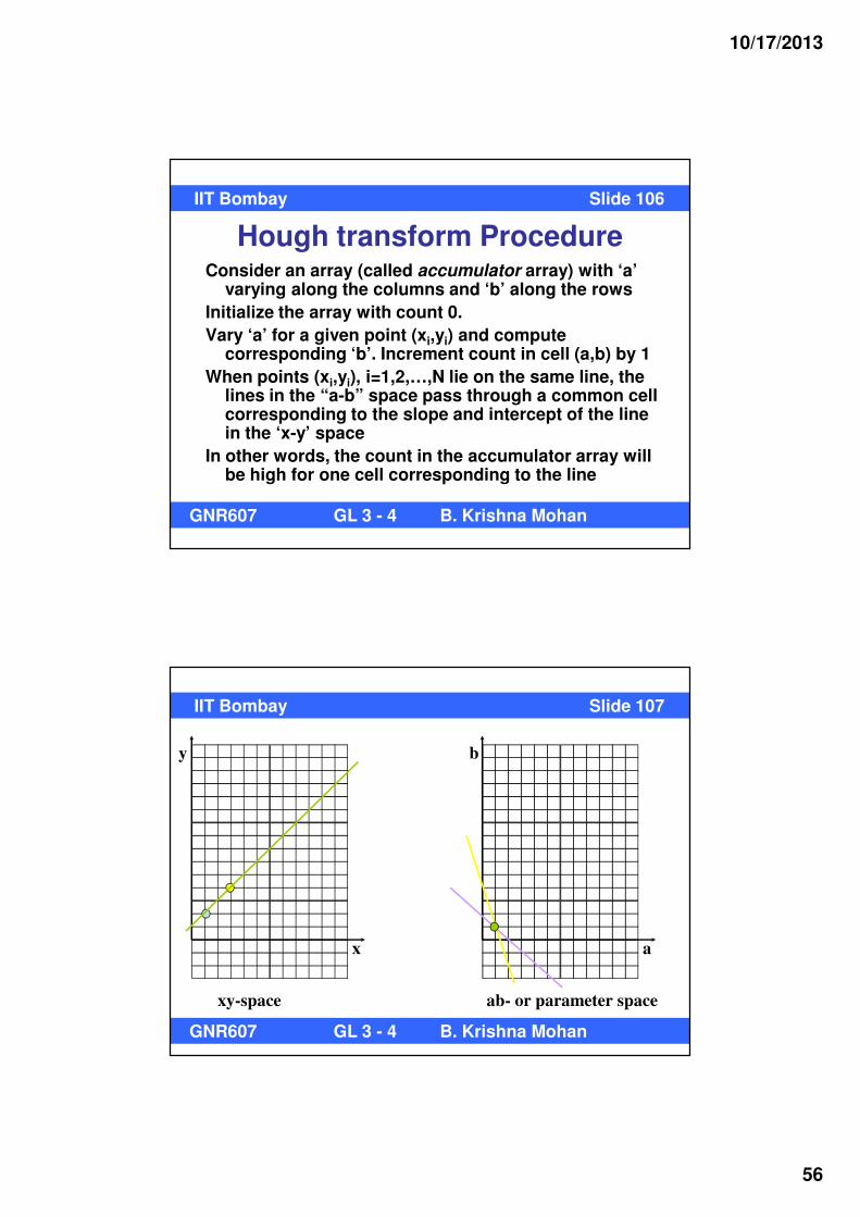
Hough transform ProcedureConsider an array (called accumulator array) with ‘a’

varying along the columns and ‘b’ along the rows

Initialize the array with count 0.

Vary ‘a’ for a given point (xi,yi) and compute corresponding ‘b’. Increment count in cell (a,b) by 1

When points (xi,yi), i=1,2,…,N lie on the same line, the lines in the “a-b” space pass through a common cell corresponding to the slope and intercept of the line in the ‘x-y’ space

In other words, the count in the accumulator array will be high for one cell corresponding to the line



y

xy-space

x

ab- or parameter space

b

a



10/17/2013

57

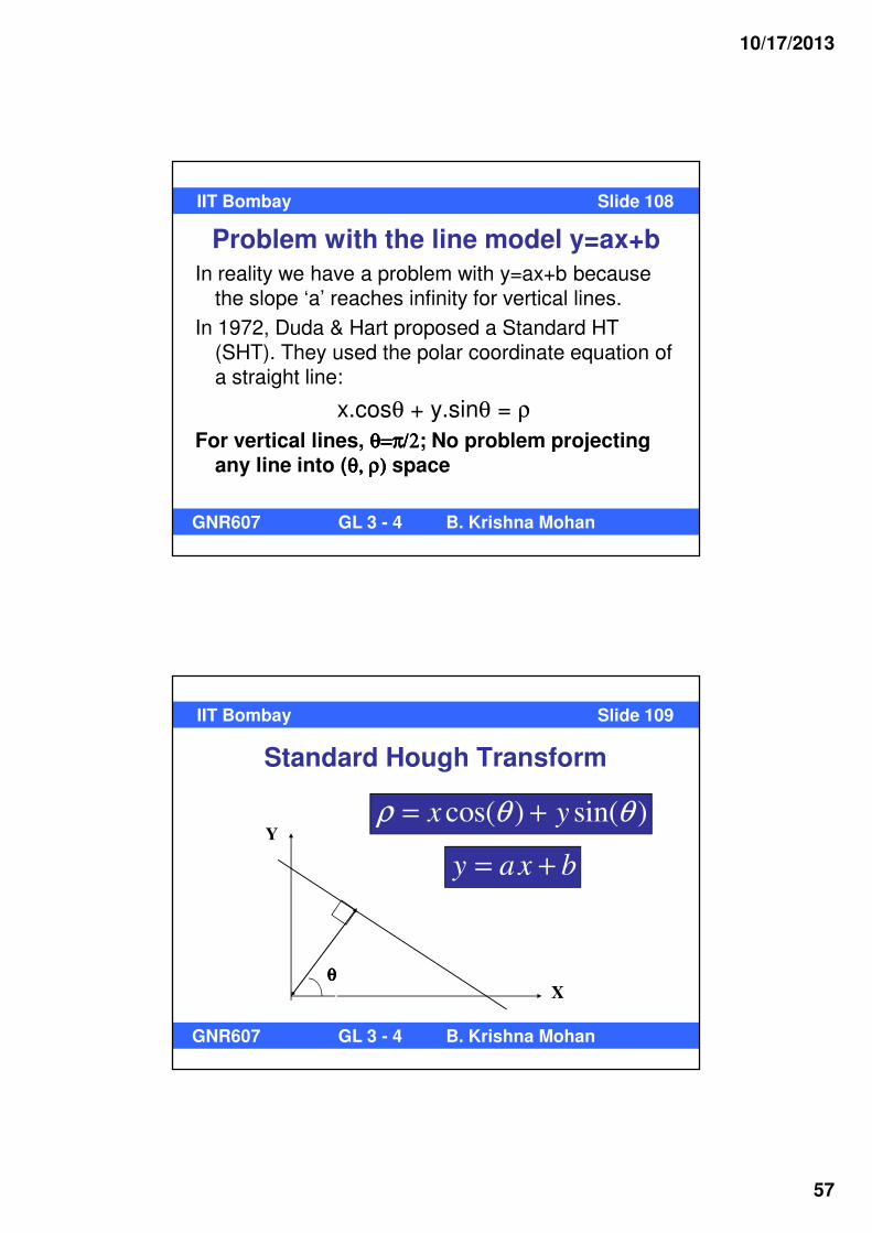
Problem with the line model y=ax+b

In reality we have a problem with y=ax+b because the slope ‘a’ reaches infinity for vertical lines.

In 1972, Duda & Hart proposed a Standard HT (SHT). They used the polar coordinate equation of a straight line:

x.cosθ + y.sinθ = ρ

For vertical lines, θ=π/2θ=π/2θ=π/2θ=π/2; No problem projecting any line into (θ, ρ)θ, ρ)θ, ρ)θ, ρ) space



Standard Hough Transform

cos( ) sin( )x yρ θ θ= +

X

Y

θθθθρ

θ

y ax b= +



10/17/2013

58

Accumulator Array CreationSelect the point (x,y) on a line

Create an array in which θθθθ varies along columns, from θ = 0 θ = 0 θ = 0 θ = 0 to θ = 2π θ = 2π θ = 2π θ = 2π in small increments (e.g., 15o)

For each θ,θ,θ,θ, find the value of ρρρρ. Increment the count in accumulator array for cell (θ,ρθ,ρθ,ρθ,ρ) by 1

For each point (x,y) there is a sinusoid in the (θ,ρθ,ρθ,ρθ,ρ) space.

All points (xi, yi) on a given line will have some (θ,ρθ,ρθ,ρθ,ρ) common





Original artwork from the book Digital Image Processing by R.C. Gonzalez and R.E. Woods © R.C. Gonzalez and R.E. Woods, reproduced with permission granted to instructors by authors on the website www.imageprocessingplace.com

Hough Space

10/17/2013

59

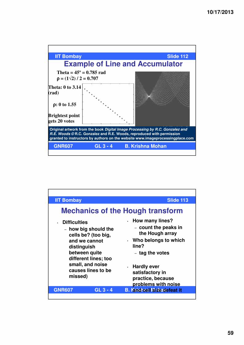
Example of Line and AccumulatorIIT Bombay Slide 112


Theta = 45º = 0.785 rad

ρρρρ = (1√2) / 2 = 0.707

Theta: 0 to 3.14 (rad)

Brightest point gets 20 votes

ρρρρ: 0 to 1.55


Mechanics of the Hough transform



• Difficulties

– how big should the cells be? (too big, and we cannot distinguish between quite different lines; too small, and noise causes lines to be missed)

• How many lines?

– count the peaks in the Hough array

• Who belongs to which line?

– tag the votes

• Hardly ever satisfactory in practice, because problems with noise and cell size defeat it

10/17/2013

60



Brightest point = 6 votes

Noisy Line


Totally Chaotic!




10/17/2013

61

Improvements to Simple Hough Transform

Noise tolerance: Most edge detectors give edge direction. Consider only those directions in accumulator array corresponding to edge direction at pixels

Speed up: A two-stage process can be considered. First, generate coarse (ρ,θ) array. Find approximate lines. Next, find precise values of (ρ,θ) by searching around the coarse values



High Order Parametric CurvesCircle: (x-a)2 + (y-b)2 = r2

Parameter space is 3-dimensionalHighly computation intensiveSearching for maxima in 3-D arrays is

computationally expensiveEfficient data structures are importantRef: A.M. Cross, Detection of circular

geological features using the Hough transform, International Journal of Remote Sensing, vol. 9, no. 9, pp. 1519-1528, 1988



10/17/2013

62

Cir

cle

Dete

cti

on



a

b

Contd…

GNR401M Remote Sensing and Image Processing - IIT …avikb/GNR401/DIP/BKM-NRM401-GL3-4... ·...

Documents

Transcript of GNR401M Remote Sensing and Image Processing - IIT …avikb/GNR401/DIP/BKM-NRM401-GL3-4... ·...