GLOTTAL EXCITATION EXTRACTION OF VOICED SPEECH - …

Clemson UniversityTigerPrints

All Dissertations Dissertations

5-2012

GLOTTAL EXCITATION EXTRACTION OFVOICED SPEECH - JOINTLY PARAMETRICAND NONPARAMETRIC APPROACHESYiqiao ChenClemson University, [email protected]

Follow this and additional works at: https://tigerprints.clemson.edu/all_dissertations

Part of the Electrical and Computer Engineering Commons

This Dissertation is brought to you for free and open access by the Dissertations at TigerPrints. It has been accepted for inclusion in All Dissertations byan authorized administrator of TigerPrints. For more information, please contact [email protected].

Recommended CitationChen, Yiqiao, "GLOTTAL EXCITATION EXTRACTION OF VOICED SPEECH - JOINTLY PARAMETRIC ANDNONPARAMETRIC APPROACHES" (2012). All Dissertations. 897.https://tigerprints.clemson.edu/all_dissertations/897

https://tigerprints.clemson.edu?utm_source=tigerprints.clemson.edu%2Fall_dissertations%2F897&utm_medium=PDF&utm_campaign=PDFCoverPages

https://tigerprints.clemson.edu/all_dissertations?utm_source=tigerprints.clemson.edu%2Fall_dissertations%2F897&utm_medium=PDF&utm_campaign=PDFCoverPages

https://tigerprints.clemson.edu/dissertations?utm_source=tigerprints.clemson.edu%2Fall_dissertations%2F897&utm_medium=PDF&utm_campaign=PDFCoverPages

https://tigerprints.clemson.edu/all_dissertations?utm_source=tigerprints.clemson.edu%2Fall_dissertations%2F897&utm_medium=PDF&utm_campaign=PDFCoverPages

http://network.bepress.com/hgg/discipline/266?utm_source=tigerprints.clemson.edu%2Fall_dissertations%2F897&utm_medium=PDF&utm_campaign=PDFCoverPages

https://tigerprints.clemson.edu/all_dissertations/897?utm_source=tigerprints.clemson.edu%2Fall_dissertations%2F897&utm_medium=PDF&utm_campaign=PDFCoverPages

mailto:[email protected]

i

GLOTTAL EXCITATION EXTRACTION OF VOICED SPEECH－

JOINTLY PARAMETRIC AND NONPARAMETRIC APPROACHES

A Dissertation

Presented to

the Graduate School of

Clemson University

In Partial Fulfillment

of the Requirements for the Degree

Doctor of Philosophy

Electrical Engineering

by

Yiqiao Chen

May, 2012

Accepted by:

John N. Gowdy, Committee Chair

Robert J. Schalkoff

Stanley T. Birchfield

Elena Dimitrova

ii

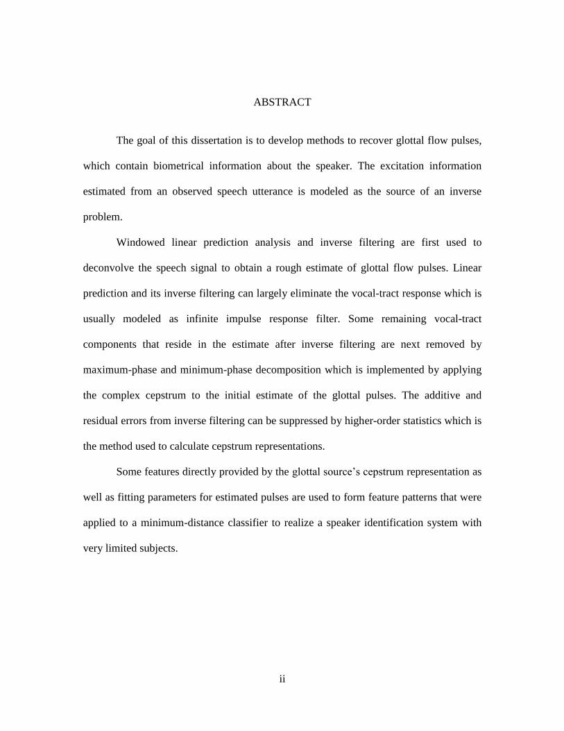
ABSTRACT

The goal of this dissertation is to develop methods to recover glottal flow pulses,

which contain biometrical information about the speaker. The excitation information

estimated from an observed speech utterance is modeled as the source of an inverse

problem.

Windowed linear prediction analysis and inverse filtering are first used to

deconvolve the speech signal to obtain a rough estimate of glottal flow pulses. Linear

prediction and its inverse filtering can largely eliminate the vocal-tract response which is

usually modeled as infinite impulse response filter. Some remaining vocal-tract

components that reside in the estimate after inverse filtering are next removed by

maximum-phase and minimum-phase decomposition which is implemented by applying

the complex cepstrum to the initial estimate of the glottal pulses. The additive and

residual errors from inverse filtering can be suppressed by higher-order statistics which is

the method used to calculate cepstrum representations.

Some features directly provided by the glottal source’s cepstrum representation as

well as fitting parameters for estimated pulses are used to form feature patterns that were

applied to a minimum-distance classifier to realize a speaker identification system with

very limited subjects.

iii

ACKNOWLEDGMENTS

I would like to appreciate the long-term support over the years provided by Dr.

John N. Gowdy, my advisor, since the first time I met him. This dissertation cannot be

completed without his guidance and patience.

Meanwhile, I wish to express my appreciation to Dr. Robert Schalkoff, Dr.

Stanley Birchfield and Dr. Elena Dimitrova for their valuable comments and helpful

suggestions in terms of this dissertation.

iv

TABLE OF CONTENTS

Page

TITLE PAGE .................................................................................................................... i

ABSTRACT ..................................................................................................................... ii

ACKNOWLEDGMENTS .............................................................................................. iii

LIST OF TABLES .......................................................................................................... vi

LIST OF FIGURES ....................................................................................................... vii

CHAPTER

I. INTRODUCTION AND OVERVIEW ......................................................... 1

Overview of Extraction of Glottal Flow Pulses ....................................... 1

Structure of the dissertation ..................................................................... 2

II. PHONETICS.................................................................................................. 4

The Physical Mechanism of Speech Production ...................................... 4

Classifications of Speech Sounds ............................................................ 7

III. MODELS ..................................................................................................... 11

Glottal Flow Pulse Modeling ................................................................. 11

Discrete-Time Modeling of Vocal Tract and Lips Radiation ................ 19

Source-Filter Model for Speech Production .......................................... 24

IV. THE ESTIMATION OF GLOTTAL SOURCE .......................................... 27

Two Methods of Linear Prediction ........................................................ 27

Homomorphic Filtering ......................................................................... 32

Glottal Closure Instants Detection ......................................................... 33

Parametric Approaches to Estimate Glottal Flow Pulses ...................... 35

Nonparametric Approaches to Estimate Glottal Flow Pulses ................ 37

v

Summary ................................................................................................ 39

V. JOINTLY PARAMETRIC AND NONPARMETRIC ESTIMATION

APPROACHES OF GLOTTAL FLOW PULSES I .............................. 40

Introduction ............................................................................................ 40

Odd-Order Linear Prediction Preprocessing and Inverse Filtering ....... 44

Phase Decomposition ............................................................................. 47

Waveform Simulations .......................................................................... 49

Simulations of Data Fitting .................................................................... 52

Summary ................................................................................................ 64

VI. JOINTLY PARAMETRIC AND NONPARMETRIC ESTIMATION

APPROACHES OF GLOTTAL FLOW PULSES II............................. 66

Brief backgrounds on High-Order Statistics .......................................... 67

Odd-Order Linear Prediction ................................................................. 69

Higher-Order Homomorphic Filtering ................................................... 72

Simulation Results ................................................................................. 77

Summary ................................................................................................ 81

VII. A SMALL SCALE SPEAKER IDENTIFIER WITH LIMITED

EXCITING INFORMATION ................................................................ 83

Overall Scheme of the Speaker Identifier .............................................. 84

Selection of Distinct Feature Patterns for Identifier .............................. 86

VIII. CONCLUSIONS.......................................................................................... 93

Jointly Parametric and Nonparametric Excitation Estimation

For Real and Synthetic Speech ........................................................ 93

Features from Estimated Glottal Pulses for Speaker Identifier ............. 95

Suggested Directions of Research ......................................................... 96

APPENDICES ............................................................................................................... 98

A: Third-Order Cumulant and Bicepstrum of Output from a Linear System

Excited by White Processes ................................................................... 99

REFERENCES ............................................................................................................ 102

vi

LIST OF TABLES

Table Page

2.1 Phonetic category of American English ........................................................ 9

5.1 Comparison of parameters of synthetic and fitting excitation pulses

from different methods .......................................................................... 63

6.1 Comparison of parameters of synthetic and fitted excitation pulses ........... 81

7.1 Speaker identification results for two different features .............................. 91

vii

LIST OF FIGURES

Figure Page

2.1 Illustration of human speech production........................................................ 5

2.2 The short-time frequency representation of a female speech utterance:

"What is the mid-way?" ........................................................................... 6

3.1 Normalized Rosenberg glottal model .......................................................... 12

3.2 Lijencrants-Fant model with shape-control parameters ............................... 14

3.3 LF models set by 3 different Rd values and their corresponding

frequency responses ............................................................................... 16

3.4 Time and frequency response of Rosenburg and LF model ........................ 17

3.5 Acoustic tube model of vocal tract .............................................................. 20

3.6 Illustration of -3 dB bandwidth between two dot lines

for a resonance frequency at 2,000 Hz................................................... 22

3.7 Resonance frequencies of a speaker’s vocal tract ........................................ 23

3.8 The discrete-time model of speech production ............................................ 26

5.1 Illustration of vocal-tract response from linear prediction analysis

with overlapped Blackman windows ..................................................... 43

5.2 Analysis region after LP analysis ................................................................ 46

5.3 Finite-length complex cepstrum of ...................................................... 48

5.4 The odd-order LP and CC flow ................................................................... 49

5.5 Estimation of glottal pulse for a real vowel /a/ ............................................ 50

5.6 Comparison between (a) Original pulse and (b) Estimated pulse ................ 51

5.7 (a) Synthetic LF excitation pulse (b) Estimated pulse (black dash line)

by LP+CC method ................................................................................. 60

viii

List of Figures (Continued)

Figure Page

5.8 Estimated pulse (black dash line) by IAIF method ...................................... 62

5.9 Estimated pulse (black dash line) by ZZT method ...................................... 62

6.1 Illustration of bispectrum of

............................................ 69

6.2 Analysis region after LP analysis ................................................................ 72

6.3 The 3rd-order cumulant of the finite-length sequence ........................... 73

6.4 Normalized GFP estimation of a real vowel /a/ ........................................... 77

6.5 Illustration of (a) Original GFP used to generate voiced Speech sequence

(b) Estimated GFP resulting from LP and bicepstrum-decomposition .. 78

6.6 Workflow to recover exciting synthetic glottal pulse .................................. 79

6.7 (a) Synthetic LF excitation pulse (b) Estimated pulse (black dash line)

and fitted pulse (gray solid line) ............................................................ 80

7.1 Speaker identification system to choose models ......................................... 85

7.2 Decision boundaries for centroids based on Minimum Euclidean

Distance.................................................................................................. 85

7.3 Illustrations of a single estimated glottal flow derivatives and their

fitting pulses ........................................................................................... 87

. 7.4 Illustrations of complex cepstrum coefficients of a single estimated glottal

flow pulse and extraction of low cepstrum-frequency quantities .......... 90

1

CHAPTER ONE

INTRODUCTION AND OVERVIEW

The topic of the dissertation, the extraction of glottal flow pulses for vowels, has a

potential benefit for a wide range of speech processing applications. Though some

progress has been made in extracting glottal source information and applying this data to

speech synthesis and recognition, there is still room for enhancement of this process. This

chapter gives a brief overview of research on this topic, and the motivation for extraction

of glottal flow pulses. The structure of the dissertation is also presented.

Overview of Extraction of Glottal Flow Pulses

The extraction of glottal flow pulses can provide important information for many

applications in the field of speech processing since it can provide information that is

specific to the speaker. This information is useful for speech synthesis, voiceprint

processing, and speaker recognition. Three major components: glottal source, vocal tract

and lips radiation, form human speech sounds based on Fant’s acoustic discoveries [1]. If

we can find a way to estimate the glottal source, the vocal-tract characteristics can be

estimated by extracting the glottal source from the observed speech utterance. As voiced

sounds are produced, the nasal cavity coupling with oral cavity is normally not a major

factor. Therefore, speech researchers focused on properties and effects of vocal-tract

response. The high percentage of voiced sounds, especially vowels, has been another

motivation for research of this domain.

2

Given observed speech signals as input data, we can formulate a task to extract

the glottal source as an inverse problem. There is no way to know what actual pulses are

like for any voiced sounds. It makes the problem much harder than those ones in

communication channels for which information source is known. Some glottal pulse

extraction methods [2], [3] have been proposed as a result of acoustic experiments and

statistical analysis. They might not be very accurate but they at least can provide rough

shapes for pulses. The earliest result came from establishing an electrical network for

glottal waveform analog inverse filtering [2]. Thereafter, some better improvements have

been made in the past two decades to recover these pulses using signal processing

methods that involve recursive algorithms for linear prediction analysis. However,

existing methods here not been able to attain both high accuracy and low complexity. The

time-variance of these excitation pulses and vocal tract expands the difficulty of the

extraction problem. The lack of genuine pulses makes it challenging for researchers to

evaluate their results accurately. In past papers [4], [5] researchers adapted the direct

shape comparison between an estimated pulse from a synthesized speech utterance and

the original synthetic excitation pulse. As part of our evaluation, we will parameterize our

estimated pulses and use these as inputs of a small scale speaker identification system.

Structure of the dissertation

The next two chapters present backgrounds for basic phonetics, glottal models

and the source-filter model as well as its discrete-time representations. After a

background discussion, we will introduce the theme of the dissertation on how to extract

3

glottal flow pulses. Mainstream glottal flow pulses estimation methods are discussed in

Chapter 4. Two jointly parametric and nonparametric methods are extensively discussed

in Chapter 5 and 6. The parameterization of estimated glottal flow pulses and their results

from a vector quantization speaker identification system with limited subjects will be

discussed in Chapter 7. Then a summary section concludes the dissertation.

4

CHAPTER TWO

PHONETICS

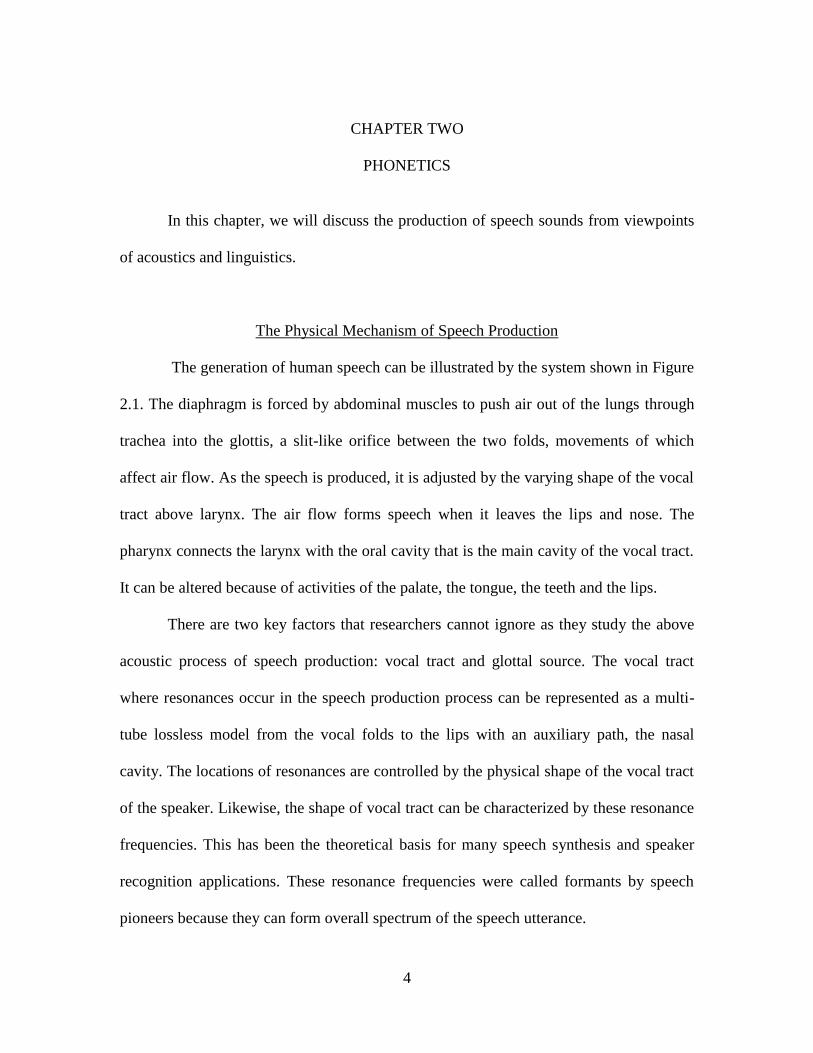
In this chapter, we will discuss the production of speech sounds from viewpoints

of acoustics and linguistics.

The Physical Mechanism of Speech Production

The generation of human speech can be illustrated by the system shown in Figure

2.1. The diaphragm is forced by abdominal muscles to push air out of the lungs through

trachea into the glottis, a slit-like orifice between the two folds, movements of which

affect air flow. As the speech is produced, it is adjusted by the varying shape of the vocal

tract above larynx. The air flow forms speech when it leaves the lips and nose. The

pharynx connects the larynx with the oral cavity that is the main cavity of the vocal tract.

It can be altered because of activities of the palate, the tongue, the teeth and the lips.

There are two key factors that researchers cannot ignore as they study the above

acoustic process of speech production: vocal tract and glottal source. The vocal tract

where resonances occur in the speech production process can be represented as a multi-

tube lossless model from the vocal folds to the lips with an auxiliary path, the nasal

cavity. The locations of resonances are controlled by the physical shape of the vocal tract

of the speaker. Likewise, the shape of vocal tract can be characterized by these resonance

frequencies. This has been the theoretical basis for many speech synthesis and speaker

recognition applications. These resonance frequencies were called formants by speech

pioneers because they can form overall spectrum of the speech utterance.

5

The formants, shown the spectrogram in the Figure 2.2, ordered from lowest

frequency to highest frequency, are symbolized by , , ,…. They are represented by

horizontal darker strips, and they vary with time. This phenomenon indicates that our

vocal tract has dynamic characteristics. The lower-frequency formants dominate the

speaker’s vocal-tract response from an energy perspective.

In above process, air flow from vocal folds results in a rhythmic open and closed

Trachea

Air Flow

from Lungs

Oral Cavity

Lips

s

Nasal Cavity

Pharyngeal Cavity

Vocal Folds

Figure 2.1 Illustration of human speech production

6

Figure 2.2 The short-time frequency representation of a female speech utterance:

"What is the mid-way?"

phase of glottal source. In the frequency domain, the glottal flow pulses are normally

characterized as a low-pass filtering response [6]. On the other hand, the time interval

between two adjacent vocal-folds opens is called pitch or fundamental period, the

reciprocal of which is called fundamental frequency. The period of glottal source is an

important physical feature of a speaker along with the vocal tract determining formants.

The glottal source in fact plays a role of excitation to both the oral and nasal

cavities. Speech has two elementary types: voiced and unvoiced, or a combination of

them [7], e.g., plosives, and voiced fricatives.

7

Voiced excitations are produced from a sort of quasi-periodic movement of vocal-

folds while air flow is forced through glottis. Consequently, a train of quasi-periodic

puffs of air occurs. The unvoiced excitation is a disordering turbulence caused by air flow

passing a narrow constriction at some point inside the vocal tract. In most cases, it can be

treated as noise. These two excitation types and their combinations can be utilized by

continuous or discrete-time models.

Classifications of Speech Sounds

In linguistics, a phoneme is the smallest unit of speech distinguishing one word

(or word element) from another. And phones triggered by glottal excitations refer to

actual sounds in a phoneme class.

We briefly list some categories of phonemes and their corresponding acoustic

features [7]:

Fricatives: Fricatives are produced by exciting the vocal tract with a stable air

flow which becomes turbulent at some point of constriction along the oral tract. There are

voiced fricatives in which vocal folds vibrate simultaneously with noise generation, e.g.,

/v/. But vocal folds in terms of unvoiced fricatives are not vibrating, e.g., /h/.

Plosives: Plosives are almost instantaneous sounds that are produced by suddenly

releasing the pressure built up behind a total constriction in the vocal tract. Vocal folds in

terms of voiced plosives vibrate, e.g., /g/. But there are no vibrations for unvoiced

plosives, e.g., /k/.

8

Affricates: Affricates are formed by rapid transitions from the oral shape

pronouncing a plosive to that pronouncing a fricative. There can be voiced, e.g., /J/, or

unvoiced, e.g., /C/.

Nasals: These are produced when there is voiced excitation and the lips are

closed, so that the sound emanates from the nose.

Vowels: These are produced by using quasi-periodic streams of air flows though

vocal folds to excite a speaker’s vocal-tract in constant shape, e.g., /u/. Different vowels

have different vocal-tract configurations of the tongue, the jaw, the velum and the lips of

the speaker. Each of the vowels is distinct from others due to their specific vocal-tract’s

shape that results in distinct resonance, locations and bandwidths.

Diphthongs: These are produced by rapid transition from the position to

pronounce one vowel to another, e.g., /W/.

The list of phonemes used in American English language is summarized in Table

2.1.

The study of vowels has been an important topic for almost any speech

applications ranging from speech and speaker recognition to language processing. There

are a number of reasons that make vowels so important.

The frequency of occurring of vowels leads them to be the major group of

subjects in the field of speech analysis. As vowels are present in any word in the English

language, researchers can find very rich information for all speech processing

applications. And they can be distinguished by locations, widths and magnitudes of

formants. These parameters are determined by the shape of a speaker’s oral cavity.

9

Finally, the glottal puffs as excitations to vowels are speaker-specific and quasi-periodic.

Intuitively, the characteristics of these pulses as glottal excitations can be considered as a

type of features [8] - [11] used for speaker recognition and other applications.

Continuant

Vowels

Front

Mid

Back

Consonants

Fricatives Voiced

Unvoiced

Whisper

Affricates

Nasals

Noncontinuant

Diphthongs

Semivowels Liquids

Glides

Consonants Voiced

Unvoiced

Table 2.1 Phonetic category of American English

However, not until some physical characteristics of speech waves were calibrated

by experiments that researchers started to assume some important properties of these

excitation signals [2]. These characteristics laid a milestone to investigate the excitation,

10

channel and lips radiation quantitatively in terms of human speech. Excitation, or glottal

sources, will be the subject through the dissertation. Some existing models of glottal

source will be extensively discussed in next chapter.

11

CHAPTER THREE

MODELS

The study of speech production has existed for several decades ago. However,

little progresses in analyzing the excitation of speech sounds had been made until some

researchers purposed methods modeling glottal flow pulses [6] - [10]. By combining the

glottal flow pulses models, glottal noise models and vocal tract resonance frequencies

transmission models, we can build an overall discrete-time speech production system.

Furthermore, the synthesis of a whole utterance of speech depends on the analysis of

interactions between glottal sources and vocal tract of speakers by using digital

processing techniques.

Glottal Flow Pulse Modeling

For voiced phonemes, typically vowels, researchers have endeavored to recover

the glottal flows to characterize and represent distinct speakers in speech synthesis and

speaker recognition. The term, glottal flow, is an acoustic expression of air flow that

interacts with vocal tract. Consequently, it is helpful to find some parameters to describe

models and regard these parameters as some features of speakers. The periodic

characteristic of the flow is determined by the periodic variation of glottis: Each period

includes an open phase, return phase and close phase. The time-domain waveform

representing volume velocity of glottal flows as excitations coming from glottis has been

an object for modeling in the past decades.

Rosenberg, Liljencrants and Fant were among those most successful pioneers who

12

contributed to find non-interactive glottal pulse models.

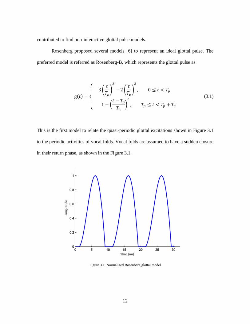
Rosenberg proposed several models [6] to represent an ideal glottal pulse. The

preferred model is referred as Rosenberg-B, which represents the glottal pulse as

( )

{

(

)

(

)

(

)

(3.1)

This is the first model to relate the quasi-periodic glottal excitations shown in Figure 3.1

to the periodic activities of vocal folds. Vocal folds are assumed to have a sudden closure

in their return phase, as shown in the Figure 3.1.

Figure 3.1 Normalized Rosenberg glottal model

13

Klatt and Klatt [9] introduced different parameters to control the Rosenberg glottal

model.

A derivative model of glottal flow pulse [10], was proposed in 1986 by Fant. The

Liljencrants-Fant (LF) model contains the parameters clearly showing the glottal open,

closed and return phases, and the speeds of glottal opening and closing. It allows for an

incomplete closure or for a return phase of growing closure rather than a sudden closure,

a discontinuity in glottal model output.

Let ( ) be a single pulse. We might assume

∫ ( )

(3.2)

then the net gain of the ( ) within both close and open phase is zero.

The derivative of ( ) can be modeled by [11]

( ) {

( ) ( )

[ ( ) ( )]

(3.3)

where and are defined in terms of a parameter by

( )

and

( ) ( )

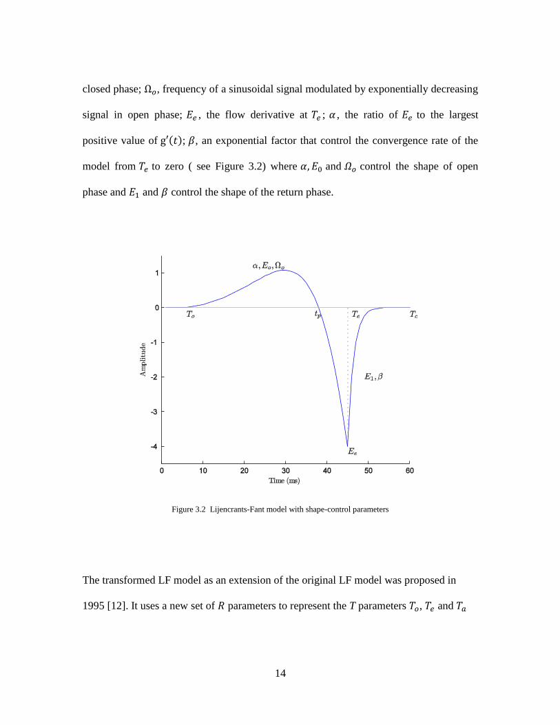
Thus, the glottal model can be expressed by 7 parameters [11]: , the starting

time of opening phase; , the starting time of return phase1; , the starting time of

1 The starting time of return phase is not defined as the peak value of a complete glottal pulse.

14

closed phase; , frequency of a sinusoidal signal modulated by exponentially decreasing

signal in open phase; , the flow derivative at ; , the ratio of to the largest

positive value of ( ); , an exponential factor that control the convergence rate of the

model from to zero ( see Figure 3.2) where and control the shape of open

phase and and control the shape of the return phase.

Figure 3.2 Lijencrants-Fant model with shape-control parameters

The transformed LF model as an extension of the original LF model was proposed in

1995 [12]. It uses a new set of parameters to represent the T parameters , and

15

involved in the LF model (effective duration of the return phase) and (the time of zero

glottal derivative). And a basic shape parameter is

( ) (

) ⁄ (3.4)

where , and are obtained as

{

(3.5)

Figure 3.3 shows a variety of LF models corresponding to different values.

The use of the parameter largely simplifies the means to control the LF model. If there

is a need for fitting a glottal flow pulse ( ) by an LF mode ( ), then a least-squares

optimization problem exists with the objective function and its constraints which can be

represented as

‖ ‖ (3.6)

subject to

Both the Rosenberg and Liljencrants-Fant models had been proved to have spectral tilt in

their frequency representations. The location of the peak of the spectral tilt is right at the

origin for a Rosenberg model and close to the origin for LF model shown in Figure 3.4.

16

Figure 3.3 LF models set by 3 different Rd values and their corresponding

frequency responses

17

Figure 3.4 Time and frequency response of Rosenburg and LF model (a) Rosenburg

model (b) Frequency response of (a) (c) LF model (d) Frequency response of (c)

18

Consequently, low-pass filtering effects in terms of the magnitude of frequency response

can be approximations to these glottal models.

After they reviewed the glottal source in the time domain and frequency domain,

Henrich, Doval and d’Alessandro proposed another Causal-Anticausal Linear Model

(CALM) [13] which considers the glottal source the impulse response of a linear filter.

They also quantitatively analyzed the spectral tilt with different model parameters.

Expressions of Rosenberg and Klatt as well as LF models were investigated in both

magnitude frequency and phase frequency domain. They proposed that the LF glottal

model itself can be regarded as a result of the convolution of two truncated signals, one

causal and one anti-causal, based on its analytical form. The open phase is contributed by

a causal signal; on the other hand, the return phase is contributed by an anti-causal signal.

Glottal flow pulse modeled by the LF model consists of minimum-phase and maximum-

phase components, so it is mixed-phase. In this case, the finite-length anti-casual signal

can be represented by zeros [13] which result in a simple polynomial rather than a ratio of

polynomials which includes poles. The existence of the discontinuity at the tail of the

return phase becomes a criterion for extracting the phase characteristic of glottal models.

Thus, the Rosenburg model is maximum-phase, but the LF model is mixed-phase.

Aspiration, which is the turbulence caused by the vibration in terms of vocal-

folds’ tense closure, is considered to introduce random glottal noise to the glottal pulse.

This may occur in a normal speech with phoneme /h/, but it seldom occurs in vowels.

19

Discrete-Time Modeling of Vocal Tract and Lips Radiation

As the major cavity involving in the production of voiced phonemes, the oral tract

has a variety of cross-sections caused by altering the tongue, teeth, lips and jaw; its

lengths varies from person to person. Fant [1] firstly modeled the vocal tract as a

frequency-selective transmission channel.

The simplest speech model consists of a single uniform lossless tube with one end

open end. The resonance frequencies of this model were called formants. The th

resonance frequency can be calculated by

( )

where is the transmission rate of the sound wave and is the length of the vocal tract as

a single tube. Therefore, the length of the vocal tract will determine the resonance

frequencies. The vocal tract was found to play a role as filter from acoustic analysis.

Some acoustics pioneers [1], [14], [15] made great contributions to investigate the

transfer function for vocal tract. This study involves a more complex but realistic model

represented by multiple concatenated lossless tubes having different cross-sectional area,

which is the extension of the single lossless tube model.

The vocal tract considered as the concatenation of tubes with different lengths and

different cross-section area , , and is shown in Figure 2.4. The cross-section

areas of tubes will determine the transmission coefficient and reflection

coefficient between adjacent tubes. (The concatenated vocal tract with

transmission and reflection coefficients ,

can be modeled by a lattice-ladder

20

discrete-time filter). The transfer function ( ) of vocal tract together with glottis and

lips can be represented by these coefficients ,

from impedance, two-port and T-

network analysis [16].

Glottis Vocal tract Lips

With discrete-time processing ( ), formants and a vocal tract consisting of

th order concatenated tubes can be modeled by the multiplication of second-order

infinite impulse response (IIR) resonance filters

( ) ( ) (

) ( ) ( ) (3.7)

where

Figure 3.5 Acoustic tube model of vocal tract

21

( )

( )( )

and , determine the location of a resonance frequencies in the discrete-time

frequency domain of ( ). As the impulse response of vocal tract ( ) is always a

BIBO stable system, we have | |, | | . Moreover, (

) can be be expressed as

(

)

| | | |

(3.8)

Then the impulse response corresponding to ( ) is

( ) | |

( )

The magnitude | | determines the decreasing rate of , and the angle determines

the frequency of modulated sinusoidal wave. So a resonance frequency can be shown

as

(

)

where is the sampling frequency for the observed continuous-time speech signal. Then

can be re-expressed as

( ) | |

( )

where ⁄ is the radian frequency of .

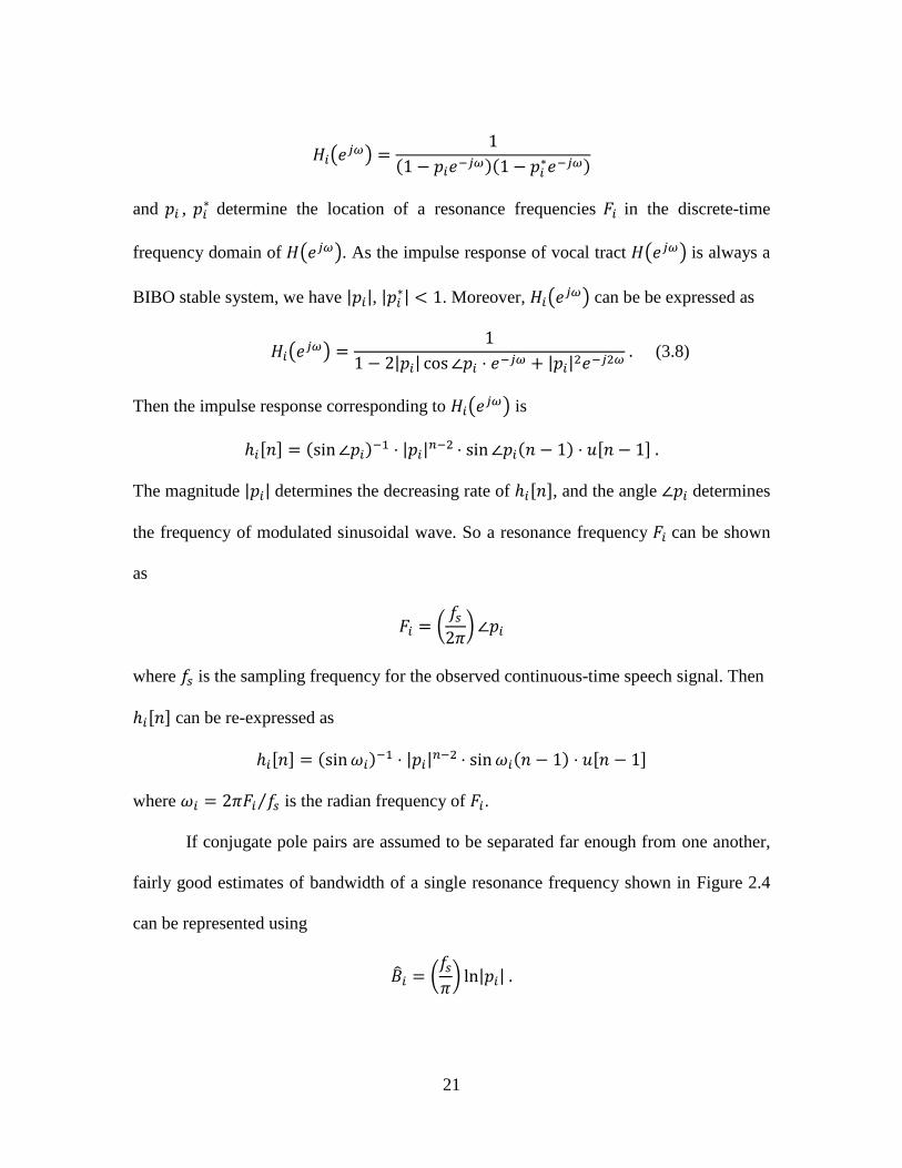
If conjugate pole pairs are assumed to be separated far enough from one another,

fairly good estimates of bandwidth of a single resonance frequency shown in Figure 2.4

can be represented using

( ) | |

22

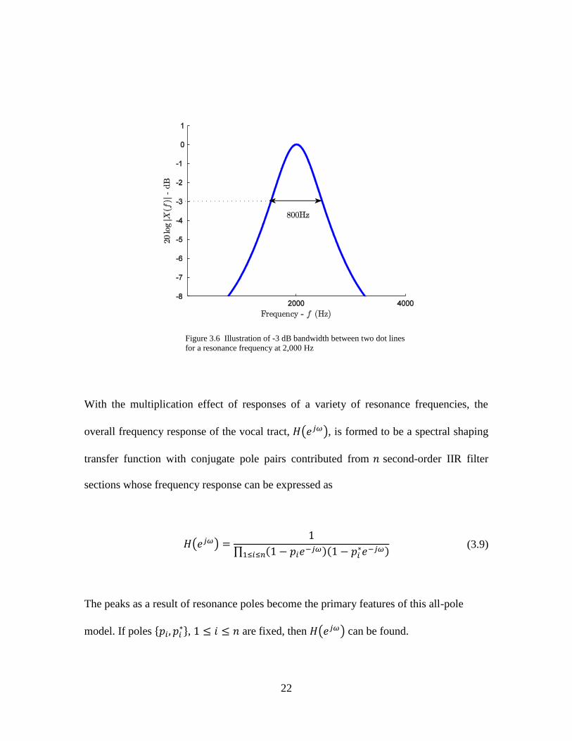
Figure 3.6 Illustration of -3 dB bandwidth between two dot lines

for a resonance frequency at 2,000 Hz

With the multiplication effect of responses of a variety of resonance frequencies, the

overall frequency response of the vocal tract, ( ), is formed to be a spectral shaping

transfer function with conjugate pole pairs contributed from second-order IIR filter

sections whose frequency response can be expressed as

( )

∏ ( )( )

(3.9)

The peaks as a result of resonance poles become the primary features of this all-pole

model. If poles { }, are fixed, then ( ) can be found.

23

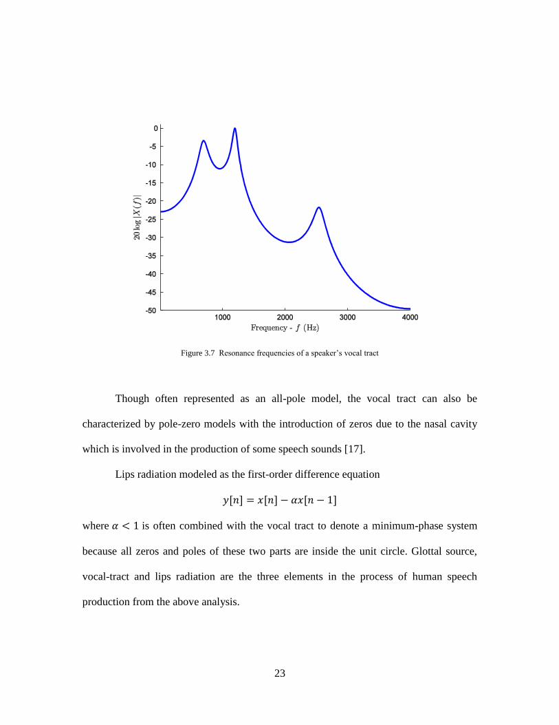
Figure 3.7 Resonance frequencies of a speaker’s vocal tract

Though often represented as an all-pole model, the vocal tract can also be

characterized by pole-zero models with the introduction of zeros due to the nasal cavity

which is involved in the production of some speech sounds [17].

Lips radiation modeled as the first-order difference equation

where is often combined with the vocal tract to denote a minimum-phase system

because all zeros and poles of these two parts are inside the unit circle. Glottal source,

vocal-tract and lips radiation are the three elements in the process of human speech

production from the above analysis.

24

Source-Filter Model for Speech Production

Now we are all set to discuss a complete model about speech production: the

source-filter model. This model serves as the key of many speech analysis methods and

applications.

Fant [1] considered that the human speech signal can be regarded as the output of

a system where the excitation signal is filtered by harmonics at resonance frequencies of

the vocal tract. This model is based on the hypothesis that the operation of acoustic

dynamics for the overall system is linear and there is no coupling or interaction between

source and the vocal tract. Time invariance is assumed. This system basically consists of

three independent blocks: periodic or non-periodic excitations (source), the vocal tract

(filter) and the effect of lips radiation.

The periodic excitations are caused by the vocal folds’ quasi-periodic vibrations.

Vowels can be considered as results of this sort of excitations. But the non-periodic

excitations are noises occurring when air is forced past a constriction. The transfer

function of vocal tract ( ) behaves as a spectral shaping function affecting the glottal

source ( ). So the observed speech signal can be represented by

( ) ( ) ( ) ( )

where ( ) denotes the lips radiation response. The above expression provides us a

frequency domain relation among these important blocks involved in the speech

production process.

25

A general discrete-time speech production model was proposed in 1978 by

Rabiner and Shafer [18]. It deems that any speech utterance can be represented by linear

convolution of glottal source, vocal tract and lips radiation shown in Figure 3.8. For

discrete-time version this model can be represented as

( ) ( ) ( ) ( ) (3.10)

It can be expanded as

( ) ( )

∏ ( )( )

( ) (3.11)

The glottal source ( ) represents white noise for unvoiced sounds and the periodic

glottal pulses for voiced sounds.

The time-domain response of the corresponding speech signal can be represented

as

( ) (3.12)

where ↔ ,

↔ ,

↔ and

↔ . The convolution relation in (3.12) as a

linear operation provides a way to decompose the observed speech signal and find

parameters to estimate signal components using digital techniques. The glottal source

signal , if it is not noise, can be recovered from the observed speech signal by

applying deconvolution. This process uses estimate of the vocal tract response

modeled as an all-pole model and lips radiation modeled as a first-order difference

equation with parameter . Properties and assumptions about glottal models

discussed in this chapter are based on the work of [1].

26

Given the overall discrete-time model of speech production in Figure 3.8,

consisting of glottal flow pulses models, all-pole and first-order difference for lips

radiation, we are able to apply digital signal processing techniques to produce a voiced

speech utterance using the glottal models introduced previously and recover glottal flow

pulses whose information is embedded in the waveforms of observed human speech

sounds. These discrete-time signal processing techniques including linear prediction and

phase separation are core aspects of the algorithms used to estimate glottal pulses in next

chapter.

Glottal flow pulses

model

Uncorrelated noise

All-pole

model 𝛼𝑒 𝑗𝜔 Voiced/Unvoiced

Figure 3.8 The discrete-time model of speech production

27

CHAPTER FOUR

THE ESTIMATION OF GLOTTAL SOURCE

This chapter is devoted to details involved in existing methods to extract glottal

waveforms of flow pulses. All these methods can be categorized into two classes: those

based on parametric models and those that are parameters free. Linear prediction is a

major tool for those belonging to the first class. The latter depends on homomorphic

filtering to implement phase decomposition as well as glottal closure instants (GCI)

detection to determine the data analysis region.

Two Methods of Linear Prediction

Until very recently, the linear prediction based methods have dominated the task

of building models to find the glottal flow pulses waveform [20], [21], [22] for different

speakers. Normally, either an estimator based on the second order statistics or an

optimization algorithm is required to find the best parameters in statistical and

optimization senses with respect to the previously chosen model. Two methods, the

autocorrelation method and the covariance method [23], are available to estimate the

parametric signal model in the minimum-mean-square estimation (MMSE) sense and the

least-squares estimation (LSE) sense, respectively. The autocorrelation method assumes

the short-time wide sense stationarity of human speech sounds to set up the Yule-Walker

equation set.

Given a th-order linear predictor and an observed quasi-stationary random

vector { } sampled from a speech signal ( ) a residual error signal is

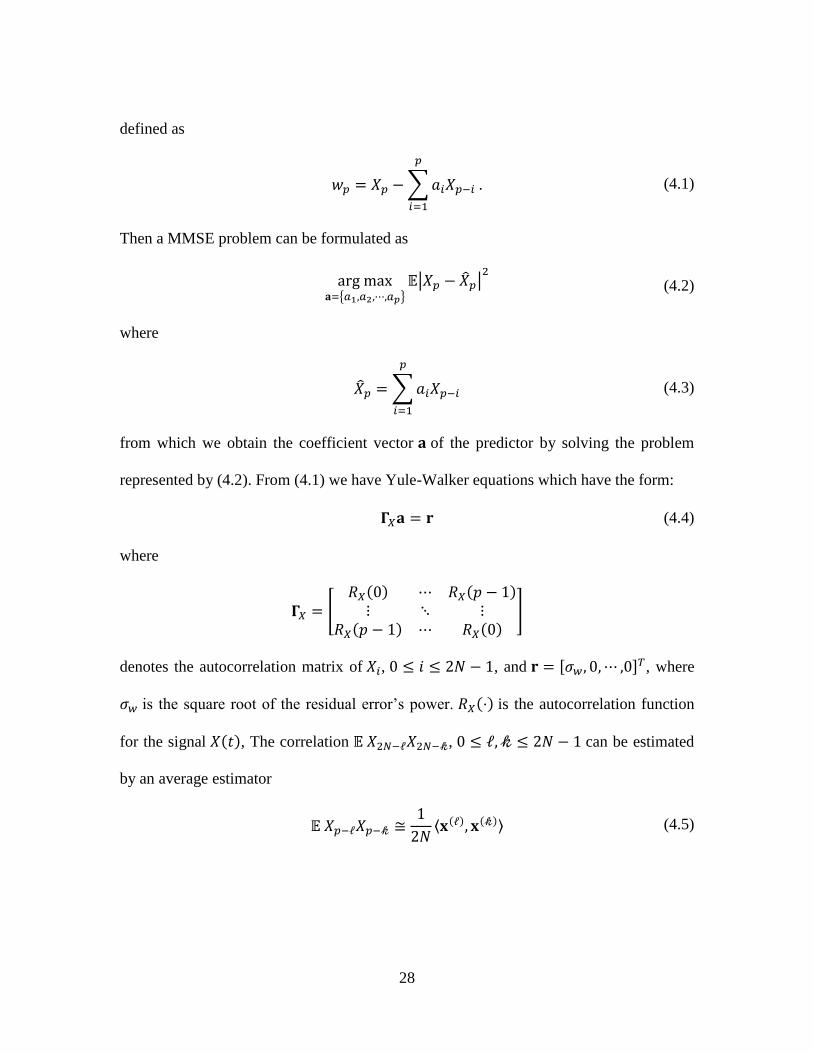
28

defined as

∑

(4.1)

Then a MMSE problem can be formulated as

{ }

| | (4.2)

where

∑

(4.3)

from which we obtain the coefficient vector of the predictor by solving the problem

represented by (4.2). From (4.1) we have Yule-Walker equations which have the form:

(4.4)

where

[ ( ) ( )

( ) ( )

]

denotes the autocorrelation matrix of , , and , where

is the square root of the residual error’s power. ( ) is the autocorrelation function

for the signal ( ), The correlation , can be estimated

by an average estimator

⟨ ( ) ( )⟩ (4.5)

29

where ( ) and ( ) denote -unit and -unit right shift of . Levinson Recursion is able

to efficiently find the optimum solution of the Yule-Walker equation set in the MSEE

sense.

In the autocorrelation method, the order of linear prediction fixes the dimension

of the Toeplitz matrix . It gives a rise to fairly large error since the order of the

predictor can’t be high. Additionally, since the autocorrelation method just minimizes the

mean-square error and requires strong stationarity for a fairly accurate second order

statistical result, it has limitations to achieving the good performance in some

environments if it is compared with the covariance method [23].

The covariance method is based on linear least-squares regression of linear

equations without relying on any statistical feature of the observed sequence. To set up its

own data matrix, the acquisition of observed data is realized by an analysis window on

the objective speech signal. As in the autocorrelation method, the dimension of columns

is uniquely determined by the order of linear prediction. But the dimension of rows for

the covariance method depends on the number of shift positions of linear predictor inside

the external analysis window. The number of rows is often larger than that of columns.

Given a th-order linear predictor and a length- analysis window of random

vector sampled from a speech signal ( ) , by shifting the

predictor inside the window we can form an data matrix which leads to solving a

problem of the form by a variety of windowing ways. Here is an over-

determined system with rank that might not equal to or . That is, can be a rank-

30

deficient matrix. A LSE problem to minimize the -norm of ‖ ‖ can be formulated

as

‖ ‖ (4.6)

There exists a method of algorithms to solve above over-determined least-squares

problem. One option is to employ Singular Value Decomposition (SVD) in its

computation [24].

The minimum -norm can also be found by decomposing shown as [25]

‖ ‖ ‖ ‖ ‖ ‖ (4.7)

where contains singular values of and are orthogonal matrices

with and [ ] . That is, and . Let

and be projections of and ; then we can obtain another equivalent

expression

‖ ‖ (4.8)

where

‖ ‖ ∑|

|

∑ | |

which is minimized if and only if

for and

for

. The least-squares solution is

∑(

)

or

31

where ∑ ( ⁄ )

is the pseudo-inverse of .

The determination of the rank of a low dimensional matrix is easy theoretically,

but it becomes more complicated in practical applications. The conventional recursive

least-squares (RLS) algorithm has been the major tool for speech processing

implementations since there doesn’t exist special consideration about the rank of . The

overall procedure can be summarized as below [25], [26]

i. Initialize the coefficient vector and the inverse correlation matrix by ( )

and ( ) where is the forgetting factor.

ii. , where is the length of the analysis window using

{ ( ) ( ) ( )

( ) ( ) ( )

we can compute the adaptation gain and update the inverse correlation matrix

( ) ( )

( )

and

( ) [ ( ) ( ) ( )]

iii. Filter the data and update coefficients

( ) ( ) ( ) ( )

and

( ) ( ) ( ) ( )

There are other versions [27], [28] of RLS algorithms used for the covariance

method to solve (4.7).

32

The autocorrelation method of MMSE has low computation costs to solve Yule-

Walker equations; however, the RLS method involves more computational costs. And it

has been proven to have better performance on voiced signals than autocorrelation

method [29]. Basically, the covariance method is considered as a pure optimization

problem; however, the autocorrelation method works on second-order statistics. These

two methods share a mutual characteristic: the model type and order for linear prediction.

For the covariance method, the length of the analysis window should be known as a priori

information.

In some cases, we need other methods, which don’t rely on any a priori

information of the given signal, to process the speech signal and extract the information

of interest.

Homomorphic Filtering

Suppose an observed sequence is the output of a system excited by a

sequence as represented by

( )

We have

( ) | ( )| ( )

which will result in phase discontinuities in the principal value of the phase at if

there exists a linear phase response in ( ).

33

From another viewpoint, let ↔ ( ) ,

↔ ( ) and

↔ ( ) then the logarithm can be applied to ( ) to separate logarithm

transformations of ( ) and ( ) as

( ) ( ) ( ) (4.9)

The cepstral relation can be obtained

( ) ( ) ( ) (4.10)

where ( ) ↔ ( ) , ( )

↔ ( ) and ( )

↔ ( ) . Based on

this relation, the linear deconvolution of and can be implemented. If ( ) and

( ) are not overlapped in the quefrency domain, then a “lifter” can be used to separate

these two cepstral representations. The deconvolution in the homomorphic domain

provides a way to discriminate a glottal-excitation response and a vocal-tract response if

their cepstral representations are separable in the quefrency domain [13], [19]. Note:

phase unwrapping is used to compensate for the issue of phase discontinuities, as

described in chapter 5.

Glottal Closure Instants Detection

In terms of voiced speech, the major acoustic excitation in the vocal tract usually

occurs at instants of vocal-fold closure defined as the glottal closure instants. Each glottal

closure indicates the beginning of the closed phase, during which there is little or no

glottal airflow through the glottis, of the volume velocity of the glottal source. The

34

detection of glottal closure instants plays an important role in extracting glottal flow

pulses synchronously and tracking the variation of acoustic features of speakers.

Automatic identification of glottal closure instants has been an important topic for

speech researchers in the past two decades. Because the measured speech signal is the

response of the vocal tract to the glottal excitation, it is a challenge to perform accurate

estimation of these instants in a recorded speech utterance.

Many methods have been proposed about this topic. A widely used approach is to

detect a sharp minimum in a signal corresponding to a linear model of speech production

[30], [31]. In [30], the detection of glottal closure instants is obtained by the lower ratio

between residual errors and original signal after the linear prediction analysis is applied

to a speech utterance. Group delay measures [30], [32] can be another method to

determine these instants hidden in the observed voiced speech sounds. They estimate the

frequency-averaged group delay with a sliding window on residual errors after linear

prediction. An improvement was achieved by employing a Dynamic Programming

Projected Phase-Slope Algorithm (DYPSA) [31]. Best results come from analysis on the

differentiated Electroglottograph (EGG) [33] (or Laryngograph signal [34]) from the

measurement of the electrical conductance of the glottis captured during speech

recordings. However, good automatic GCI detection methods with better estimations

have a high computation cost.

35

Parametric Approaches to Estimate Glottal Flow Pulses

Applications of covariance analysis to the problem of extraction of glottal flow

pulses have been performed successfully for short voiced phoneme utterances by some

researchers [20], [21]. All parametric estimation methods to extract glottal flow pulses

have three components: application of linear prediction analysis, normally using the

covariance method; selection of the optimum linear prediction coefficients set to

represent the vocal-tract response; and deconvolution of the original speech using

estimated linear prediction coefficients to extract glottal flow pulses.

Wong, Markel and Gray proposed the first parametric approach [21] using

covariance analysis. Their approach can be summarized as follows. Assume an all-pole

model ( ) for the vocal-tract and fix the model order. The size of an analysis frame is

selected to ensure that the sliding window has all data needed between the two ends of

the analysis frame. Then set up an over-determined system using data inside all sliding

windows and employ the least square algorithm to find the optimum parameters. Then the

parameter set and the -norm of the residual error vector are both recorded

corresponding to the current specific location of the sliding window. Finally, access the

recorded parameters corresponding to the location where the power ratio between

residual errors and the original signal is minimized. Consequently, that chosen parameter

set is used to form the inverse system of the vocal-tract model, through which the inverse

filtering for deconvolution is applied to the original speech sequence. The result of the

operation is the combination of the glottal pulse and lips radiation. Furthermore, we can

estimate the glottal pulse waveform by removing lips radiation ( ) from the overall

36

response of the speech utterance denoted by ( ). The procedure for estimating the

glottal pulse is described by

{ ( ) ( ) ( )} (4.11)

The mismatch of locating the glottal closure phase estimated as above will introduce

inaccuracies to the final estimation of pulses.

Alku proposed another method [4], iterative adaptive inverse filtering (IAIF), to

extract glottal flow pulses by two iterations. It requires a priori knowledge about the

shape of the vocal tract transfer function which can be firstly estimated by covariance

analysis of linear prediction after the tilting effect of glottal pulse in frequency domain

has been eliminated from the observed speech. In the first iteration, the effect of the

glottal source estimated by a first-order linear prediction all-pole model was used to

inverse filter the observed speech signal. A higher-order covariance analysis was applied

to the resulting signal after inverse filtering. Then a second coarse estimate is obtained by

integration to remove the lips radiation from last inverse filtering result. Another two

rounds of covariance analysis are applied in a second process. Correspondingly, two

inverse-filtering procedures are involved in the whole iteration. A refined glottal flow

pulse is estimated after another stage of lips radiation cancellation. Compared with the

previous method, an improvement in the quality of estimation has been achieved with a

sophisticated process, in which four stages of linear prediction have been used.

In addition to these two approaches based on all-pole models, there are other

approaches based on different model types [22]. Using a priori information about model

type and order, these parametric methods can estimate and eliminate the vocal-tract

37

response. However, the number of resonance frequencies needed to represent a specific

speaker and his pronounced phonemes is unknown. This uncertainty about orders of the

all-pole model might largely affect the accuracy of the estimation of the vocal-tract

response. Some researchers found another way to extract the glottal excitations to

circumvent these uncertainties about linear prediction models. These are summarized

below.

Nonparametric Approaches to Estimate Glottal Flow Pulses

The LF model has been widely accepted as a method for representing the

excitation for voiced sounds since it contains an asymptotically closing phase to

correspond to the activity of speaker’s closing glottis.

The LF model’s closed and open phases have been shown to consist of

contributions by maximum-phase components [13]. The LF model offers an opportunity

to use nonparametric models to recover an individual pulse. Meanwhile, a linear system’s

phase information becomes indispensable in the task of glottal pulse estimation. The

Zeros of -transform (ZZT) method and the complex cepstrum (CC) method [19], [20]

have been applied to the speech waveform present within one period of vocal-folds

between closed phases of two adjacent pulses. Then maximum-phase and minimum-

phase components can be classified as the source (glottal pulse) and tract (vocal-tract)

response, respectively. For nonparametric approaches the vocal tract is considered to be

contributing only to the minimum-phase components of the objective sequence. And

maximum-phase components correspond to the glottal pulse.

38

It has been recognized that human speech is a mixed-phase signal where the

maximum-phase contributions corresponds to the glottal open phase while the vocal tract

component is assumed to be minimum-phase. The “zeros of the -transform” method [19]

technique can be used to achieve causal and anti-causal decomposition.

It has been discussed that the complex cepstrum representation can be used for

source-tract deconvolution based on pitch-length duration with glottal closure as its two

ends. But there are some weaknesses in terms of nonparametric methods as discussed

below.

The pinpoint of the two instants to fix the analysis region will be necessary for all

these existing nonparametric methods. Although there have been some glottal closure

instants detection algorithms proposed, selecting the closed phase portion of the speech

waveform has still been a challenge to ensure the high-quality glottal closure instants

detection. This adds computational costs to the estimation of glottal flow pulses. On the

other hand, the minimum-phase and maximum-phase separation assumes the finite-length

sequence is contributed by zeros which contradicts the fact that vocal-tract response is

usually regarded as the summation of infinite attenuating sinusoidal sequences that might

be longer than one pitch.

Any finite-length speech utterance can be viewed as the impulse response of

a linear system containing both maximum-phase and minimum-phase components. The

-transform of the signal can be represented as

( ) ∏ (

) ∏ ( )

∏ ( )( )

(4.12)

39

where { } { } { } all have magnitude less than one and is the linear phase

terms as the result of maximum-phase zeros.

With the homomorphic filtering operation, the human speech utterance as a

system response can be separated into maximum and minimum phase components. The

factors of ( ) are classified into time-domain responses contributed by maximum-phase

and minimum-phase components. Then both maximum-phase and minimum-phase parts

can be separated by calculating the complex cepstrum of the speech signal

during adjacent vocal fold periods. As we indicated before, pitch detection will be needed

to ensure those two types of phase information can be included in the analysis window.

Summary

In this chapter, we summarized both parametric and nonparametric methods

involving linear prediction, homomorphic filtering, and GCI detection to estimate glottal

flow pulses from a voiced sound excited by periodic glottal flow pulses. However, these

two major classes of methods have their own weaknesses caused by the characteristics of

these respective processing schemes. These weaknesses sometimes can largely reduce the

accuracies of the estimation of pulses and introduce distortions to them. For the

remaining chapters, the challenge confronting us changes from extracting excitation

pulses to preserving recognizable features of pulses with the largest possible fidelity.

40

CHAPTER FIVE

JOINTLY PARAMETRIC AND NONPARMETRIC ESTIMATION

APPROACHES OF GLOTTAL FLOW PULSES I

Linear prediction and complex cepstrum approaches have been shown to be

effective for extracting glottal flow pulses. However, all of these approaches have their

limited effectiveness. After the weaknesses of both parametric and nonparametric

methods [17], [18], [19] presented had been considered seriously, a new hybrid

estimation scheme is proposed in this chapter. It employs an odd-order LP analyzer to

find parameters of an all-pole model by least-squares methods and obtains the coarse

GFP by deconvolution. It then applies CC analysis to refine the GFP by eliminating the

remaining minimum-phase information contained in the glottal source estimated by the

first step.

Introduction

We present here a jointly parametric and nonparametric approach to use an odd-

order all-pole predictor to implement the LP analysis. Covariance methods of linear

prediction analysis typically based on all-pole models representing the human vocal tract

once dominated the task of glottal pulse extraction [20], [21]. They adapted a least-square

optimization algorithm to find parameters for their models given the order of models, and

the presence or absence of zeros. These models with a priori information involve strong

assumptions, which ignore some other information that might be potentially helpful for

more accurate separation.

41

The introduction of the residual errors from LP analysis, normally regarded as

Gaussian noise, affects the glottal pulse extraction results. On the other hand, an

individual LF model [10], [12] has a return phase corresponding to the minimum-phase

components [19]. The return phase can recovered by polynomial roots analysis. This

method can be used to perform decomposition of the maximum-phase part and minimum-

phase part of speech signals. Decomposition results have proven helpful for achieving the

source-tract separation. The decompositions are carried out on a finite-length windowed

speech sequence where the window end points are set to the glottal closure instants [19],

[35]. ZZT and CC, which involve polynomial factorization are effective for the

decomposition in terms of the phase information of the finite-length speech sequence.

There are two factors that might affect the final separation results. The finite number of

zeros might be insufficient to represent the vocal tract. Also, accurate detection of GCIs

involves high computation costs.

If the vocal-tract is not lossless [17], it is assumed to be minimum-phase and

represented by complex conjugate poles of an all-pole model. Any individual glottal

pulse is forced to be represented using at least one real pole from the model.

Based on the above consideration, we refined previous separation results using the

CC to realize the phase decomposition. Simulation results shown later in this chapter

demonstrate that, compared with existing parametric and nonparametric approaches, the

presented approach has better performance to extract the glottal source.

The vocal-tract is assumed to be a minimum-phase system represented by

complex conjugate poles of an all-pole model. With extending the covariance analysis

42

window, the variance coming from different locations of the window will be largely

reduced as Figure 5.1 shows. We can therefore utilize the covariance methods in the

normal LP analysis applications free of sensitive location of the window [36], [37].

Therefore, any individual glottal pulse is forced to be represented using at least one real

pole in the LS regression process. Then we refined separation results with CC to realize

the phase decomposition.

Based on the estimated performance for both synthetic and real speech utterances,

our simulation results demonstrate, like existing completely parametric and

nonparametric approaches, that the presented approach also has effective and promising

performance to extract the glottal flow pulses. Additionally, the new approach won’t

consume much computational resource.

43

Figure 5.1 Illustration of vocal-tract response from linear prediction

analysis with overlapped Blackman windows

44

Odd-Order Linear Prediction Preprocessing and Inverse Filtering

Consider the voiced speech signal for which the -transform is denoted by

( ) ( ) ( ) (5.1)

where ( ) is response of glottal flow pulses (GFPs) and the lip radiation, and ( ) is

the response of vocal tract that is a minimum-phase system and it might contain zeros.

( ) can be represented by

( ) ( ) ( )

Here ( ) denotes all-zero part and ( ) denotes all-pole part of the vocal-tract

response. The determination of ( ) and ( ) leads to the source-tract separation.

Covariance methods of LP analysis, usually with even order, have become a

major tool for the parametric analysis of voiced speech utterances. On the other hand, an

odd-order all-pole model expressed by

( )

∑

guarantees that at least one real pole is included to represent the low-pass tilting effect of

the glottal source. We can separate ( ) into two systems ( ) contributed by

complex pole pairs and ( ) contributed by real poles.

Let [ ( )

( )

]

be a windowed discrete-time speech frame and

be the optimum estimate of in the Least-Squares (LS) sense. Then the all-

pole model coefficients vector [ ( )

( )

]

is found to minimize the norm

error between the observed signal and its estimate . In general,

45

‖ ‖ (5.2)

where ( ) is defined by

[

( )

( )

( )

( )

( )

( )

( )

( )

( )

( )

( )

( )

]

(5.3)

which is a data matrix formed with a shifted version of the current observation data frame;

and can be determined by recursive LS algorithms.

Given a predictor coefficient vector with odd elements, there exists at least one

real root , such that

( ) ∑

as the result of LS estimation. Then the remaining complex poles , excluding

from the set , are reserved for the representation of the coarse vocal-tract response.

Here is the set of all roots of the above polynomial.

These estimated complex conjugate poles further form a linear filter which can be

used to deconvolve the observed speech signal to obtain the coarse representation of the

glottal source corresponding to the current speech frame. Thus, it results in the estimated

glottal excitation ↔ ( ) expressed by

( ) ( )

( ) ( ) ( ) ( ) ( ) (5.4)

where ( ) on the right hand side of (7) can be further expressed by

46

( ) ( )

( ) (5.5)

which denotes the ratio between ( ) and its estimate ( ). Because

| | , , ( ) is minimum-phase. The ratio ( ) is a minimum-phase

system as well. Therefore, the coarse estimate of GFPs will still be a mixed-phase system

affected by cancelling effects of the ratio between ( ) and ( ). A new

estimate can be defined by

( ) (5.6)

where is an individual glottal pulse, is the error introduced by the inverse

filtering and is an impulse train defined by

∑

(5.7)

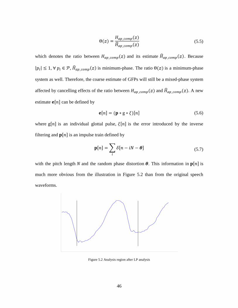
with the pitch length and the random phase distortion . This information in is

much more obvious from the illustration in Figure 5.2 than from the original speech

waveforms.

Figure 5.2 Analysis region after LP analysis

47

This enables us to employ a simpler system to obtain the GFP information using the

phase decomposition to extract the minimum phase parts in which is mixed-phase.

Phase Decomposition

Results from the covariance method of odd-order LP analysis form a good

foundation for further processing. After the inverse filtering, phase decomposition can be

used to refine the estimate of the glottal pulse by removing the minimum-phase part. It

also can be used for synchronized GFP recovery.

Fixing for each pulse, we are able to detect the glottal closure instants in

for its pulses’ refinements. Let be a portion of the glottal excitation between

two adjacent GCIs and ↔ ( ) where

( ) (5.8)

can be analyzed by homomorphic filtering to separate the minimum-phase

and maximum-phase sequences. The region between the two solid lines in Figure 5.2 for

CC analysis spans slightly longer than one pitch between two GCIs. Notice the tilting

effect due to the bias [21].

After phase unwrapping and determination of the algebraic sign of the gain of

( ), the computation of the finite-length CC of , which can be regarded as a higher-

order polynomial can be performed using [23]

48

{ ( ) }

{

| |

∑

∑

(5.9)

where coefficients and are the polynomial’s minimum-phase roots and maximum-

phase roots’ reciprocals, respectively. The quantities of the cepstrum representation on

the left side of the origin contribute to the maximum-phase components of for the

current pulse. Due to time-domain aliasing, the low-index terms of the maximum-phase

components are not taken into account for the following inverse transform to recover the

current GFP. As shown in Figure 5.3 round dots for the maximum-phase are reserved as

the input for the following operation that converts the response from the cepstrum

domain back to the time-domain.

Figure 5.3 Finite-length complex cepstrum of . (Round dots

will be reserved for the inverse transform to recover the pulse.)

49

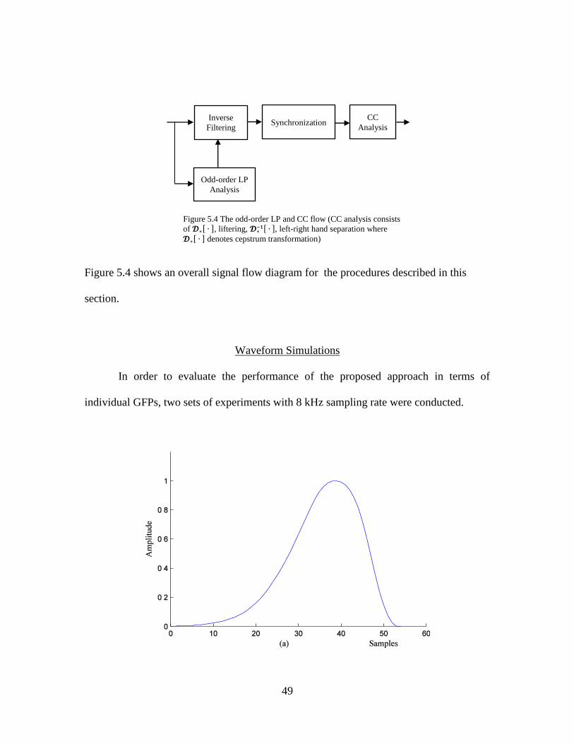
Figure 5.4 shows an overall signal flow diagram for the procedures described in this

section.

Waveform Simulations

In order to evaluate the performance of the proposed approach in terms of

individual GFPs, two sets of experiments with 8 kHz sampling rate were conducted.

CC

Analysis

Inverse

Filtering

Odd-order LP

Analysis

Synchronization

Figure 5.4 The odd-order LP and CC flow (CC analysis consists

of 𝓓 , liftering, 𝓓 −𝟏 , left-right hand separation where

𝓓 denotes cepstrum transformation)

50

Figure 5.5 Estimation of glottal pulse for a real vowel /a/. (a) Normalized GFP

(b) Derivative waveform

Figure 5.5 shows the estimation of an individual GFP and its derivative waveform

for a real vowel from a male speaker after 13th-order LP analysis and phase

decomposition. We notice the smooth curve occurring at the tail of the return phase of the

glottal flow pulses in (a).. In Figure 5.5(b), the derivative of the signal of Figure 5.5(a)

demonstrates the effects of lips radiation.

Another individual glottal flow pulse estimated for a synthetic voice sound

generated by source-filter model is shown in Figure 5.6. The original glottal flow pulses

were synthesized by the convolution of two exponential sequences [39] which guarantees

the generated individual glottal flow pulses are of maximum-phase. Six pairs of complex

conjugate poles were used to represent the vocal-tract response. Based on Figure 5.6(a)

there is no curve present in the tail of the return phase. Note that a time shift occurs in

51

Figure 5.6(b), and there are some subtle distortions present in the open phase compared

with Figure 5.6(a).

Figure 5.6 Comparison between (a) Original pulse and (b) Estimated pulse

52

Though the above comparison in Figure 5.6(a) and Figure 5.6(b) is direct, it is

still an intuitive evaluation of our approach based on checking the difference between

waveforms.

Simulations of Data Fitting

We can formulate a nonlinear least-square problem to evaluate the performance of

the extraction approach by following steps:

Use LF pulses determined by a fixed parameter sets to produce excitation pulses.

Then apply the excitation pulses to artificial vocal-tract response modeled by several

pairs of complex conjugate poles to generate a speech signal. Next, employ the

estimation approach to recover the original glottal derivative pulse used. Comparing the

nonlinear LS fitting result of estimation with the original synthetic

LF derivative pulses, we can make the evaluation more quantitatively than before.

Let be the discrete form of derivative pulse (see equation (3.3)) fitting the estimated

pulse [39] by our approach. Then we can formulate an objective value which is defined

by

‖ ‖

∑| |

∑

∑ { ( ) ( ) }

∑ { [ ( ) ( )]}

53

(5.10)

where and are discrete correspondances of and ;

( ) ⁄

and

( ) ( ) ⁄ .

So the objective function is formulated as

There are many potential algorithms to solve this nonlinear programming LS

problem [40] - [47]. However, some standard optimization methods, like Gauss–Newton

with convenient and effective approximations for the Hessians, are not good candidates

for a large that might give rise to a rank-deficient Jacobian matrix occurring in

iterations for the current piecewise data-fitting problem [11], [48]. This sort of weakness

can be overcome by the introduction of a trust-region strategy.

The Levenberg-Marquardt method [49] - [51] or other Trust-Region methods [52]

-[60] using the trust-region framework work well concerning this optimization case,

especially the Interior-Point Trust-Region version, which were used in our experiments

about nonlinear fitting. They can be regarded as an improvement on the limited memory

quasi-Newton [52] method within trust regions.

The Interior-Point Trust-Region approach defines a region, normally represented

by distance from the current reference point. The next stage of iteration is constrained

to be within this region to present an overly long step from the current reference point.

An objective function modeled within this region chooses the direction and size

54

simultaneously for the next step. If the next potential step is not successful, the method

will adaptively reduce the size of current region and formulate the next minimizer. On the

other hand, if the potential step is successful, the size of the current region will be

enlarged. The size of the trust region is central to each step. The objective function value

won’t move much closer to the minimum point in the next step if the region is too small;

otherwise, the objective function value of the model will be far from the minimum point

of the objective function. Thus, the previous iteration’s performance will uniquely

determine the size of the region. A successful step explained below indicates that the

current model is good over the current region and its size can be increased. A failed step

indicates that the current modeling of the objective function is an inadequate expression

of the objective function, and then the step size will be decreased.

A trust-region method will yield longer steps and a larger reduction in the

function to be minimized, towards its potential minimum point in its trust region, than

line search methods. With the iterations and adjustments of the trust region included in

the optimization procedure, the algorithm converges to the local extreme value in the

trust region.

For a nonlinear objective function

{ ( ) } (5.11)

is the objective function with lower and upper bounds interior with a

feasible set { } where is an interior box-bounded region. Thus,

the scaled feasible point maintains the equivalent unit distance to all nearest bounds in

the region . Distance can be determined using

55

( ) (5.12)

where

( )

More flexibility is provided for reducing the value of the objective function [61] - [65].

By Taylor’s theorem associated with the objective function at a value , we

have the expression

( ) ( ) [ ( )

]

[ ( )

]

where and the term ( )

[ ( )

] is the mean-value

form of remainder. Then we are seeking the solution to the subproblem below for the th

step

{ ( ) [ ( )

]

[ ( )

] ‖ ‖ } (5.13)

where within a sufficiently small neighborhood of elliptical trust region

‖ ‖ centered at for current variable ; is a scaling matrix and is the

size of trust region.

Combining both lower and upper bounds of , a new function can

be defined by

56

( )( )

{

( ) ( )

( )

( ) ( )

( ) ( ) ( )

( ) ( )

( )

( ) ( )

( )

( ) ( )

(5.14)

Let be a diagonal matrix for affine scaling such that

( √| ( )|⁄ ) (5.15)

Then

( )

will be the solution to the above subproblem if the trust region size is sufficiently

large in the interior neighborhood of a local minimizer. By the affine transformation,

we have

,

(| ( )| )

and

( )

( )

where is the Jacobian for | ( )|, is an approximation for

( )

and

( )

where is a positive semi-definite diagonal matrix that contains the information of

constraints.

57

The nonlinear function

( ) ( )

can be approximated by the quadratic ( ) using the Taylor Theorem. Let

; then

{ ( ) ( )

( ( )

) ‖ ‖ } (5.16)

where

( )

In the neighborhood of a local minimum value, the Newton step [66] used to solve

( )

is in fact a solution to the above trust-region problem if is sufficiently

large.

Then the trust region is computed for use in the th step or iteration. Since

( ) is an approximation to ( ) ( )

, the size of trust region

would be updated by a rule based on a degree of approximation that can be

measured by the ratio between actual reduction of and predictive reduction of :

( ) ( )

( ) ( ) (5.17)

If which is a predefined threshold between 0 and 1, the current trust region will

be enlarged by adjusting to indicate that the objective function was reduced

successfully at the th step. If , then the trust region would be compacted to imply

58

that the objective function was not reduced successfully at the th step. The overall

procedure can be summarized in [53] as below:

Initialization: Find a point for

For

1. Find ( ), , , and .

2. Compute as an approximate solution based on the quadratic model

( )

( )

to ensure .

3. Compute .

4. If , then set . Otherwise, let .

5. Update and .

6. Repeat, stating at stage 1.

The convergence analysis of the above algorithm is shown in [53].

For an arbitrary single pulse estimated by different approaches ranging from

LP+CC, IAIF to ZZT to be fitted by Trust-Region methods, the pulse will be aligned with

the location - of the maximum negative value of the glottal pulse in Figure 5.7(a) and

normalized by dividing the value of the flow derivative at - . Then the fitting

operation is applied to the normalized version of the estimated waveform with fixed.

To minimize the error, the shifted and normalized version is nonlinearly fitted by

fixing the location of and normalizing the amplitude of at according to the

procedure summarized above. Furthermore, the estimated and fitted waveforms spanning

59

an interval of one pitch period will be parameterized quantitatively if the data fitting

process converges successfully [67] - [73] by the above nonlinear least-square optimizer

with or without constraint about net gain of the overall fitting pulse shape. By comparing

the predetermined parameter set for generating the LF excitation pulse and the parameter

values resulting in the fitting pulses, we can evaluate the estimation performance with a

variety of approaches listed before. The parameters associated with different methods are

summarized in Table 5.1.

60

Figure 5.7 (a) Synthetic LF excitation pulse (b) Estimated pulse (black dash line) by LP+CC method

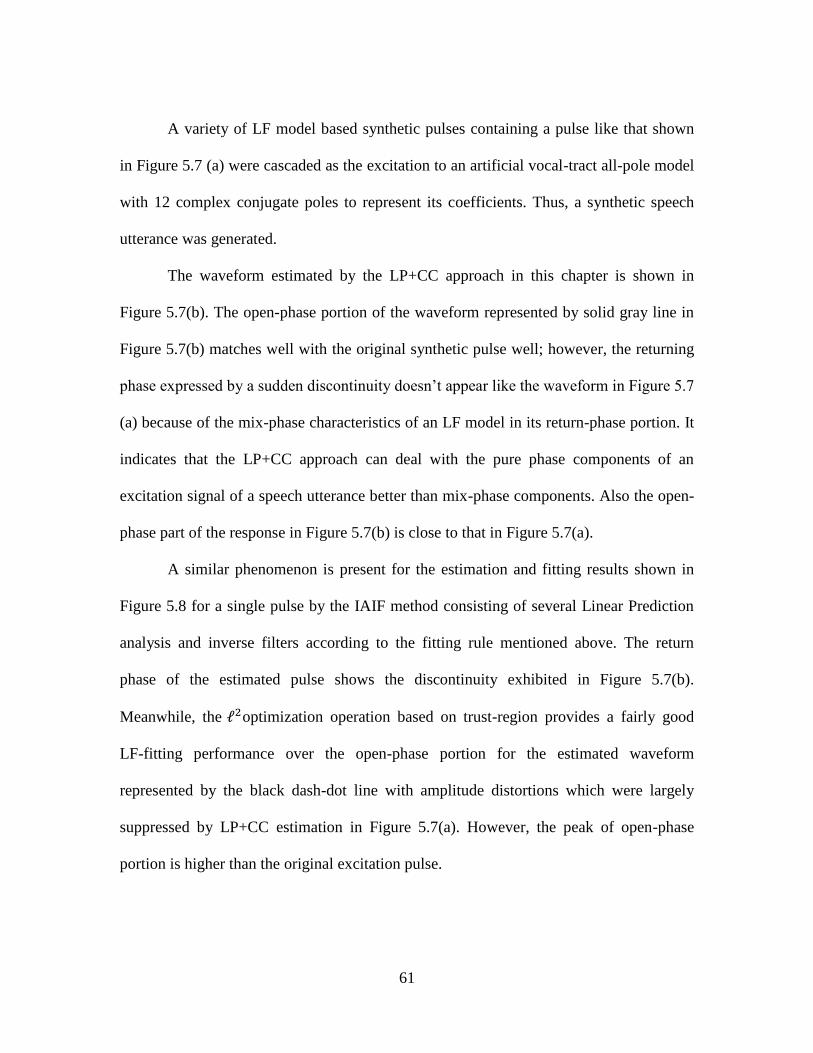
61

A variety of LF model based synthetic pulses containing a pulse like that shown

in Figure 5.7 (a) were cascaded as the excitation to an artificial vocal-tract all-pole model

with 12 complex conjugate poles to represent its coefficients. Thus, a synthetic speech

utterance was generated.

The waveform estimated by the LP+CC approach in this chapter is shown in

Figure 5.7(b). The open-phase portion of the waveform represented by solid gray line in

Figure 5.7(b) matches well with the original synthetic pulse well; however, the returning

phase expressed by a sudden discontinuity doesn’t appear like the waveform in Figure 5.7

(a) because of the mix-phase characteristics of an LF model in its return-phase portion. It

indicates that the LP+CC approach can deal with the pure phase components of an

excitation signal of a speech utterance better than mix-phase components. Also the open-

phase part of the response in Figure 5.7(b) is close to that in Figure 5.7(a).

A similar phenomenon is present for the estimation and fitting results shown in

Figure 5.8 for a single pulse by the IAIF method consisting of several Linear Prediction

analysis and inverse filters according to the fitting rule mentioned above. The return

phase of the estimated pulse shows the discontinuity exhibited in Figure 5.7(b).

Meanwhile, the optimization operation based on trust-region provides a fairly good

LF-fitting performance over the open-phase portion for the estimated waveform

represented by the black dash-dot line with amplitude distortions which were largely

suppressed by LP+CC estimation in Figure 5.7(a). However, the peak of open-phase

portion is higher than the original excitation pulse.

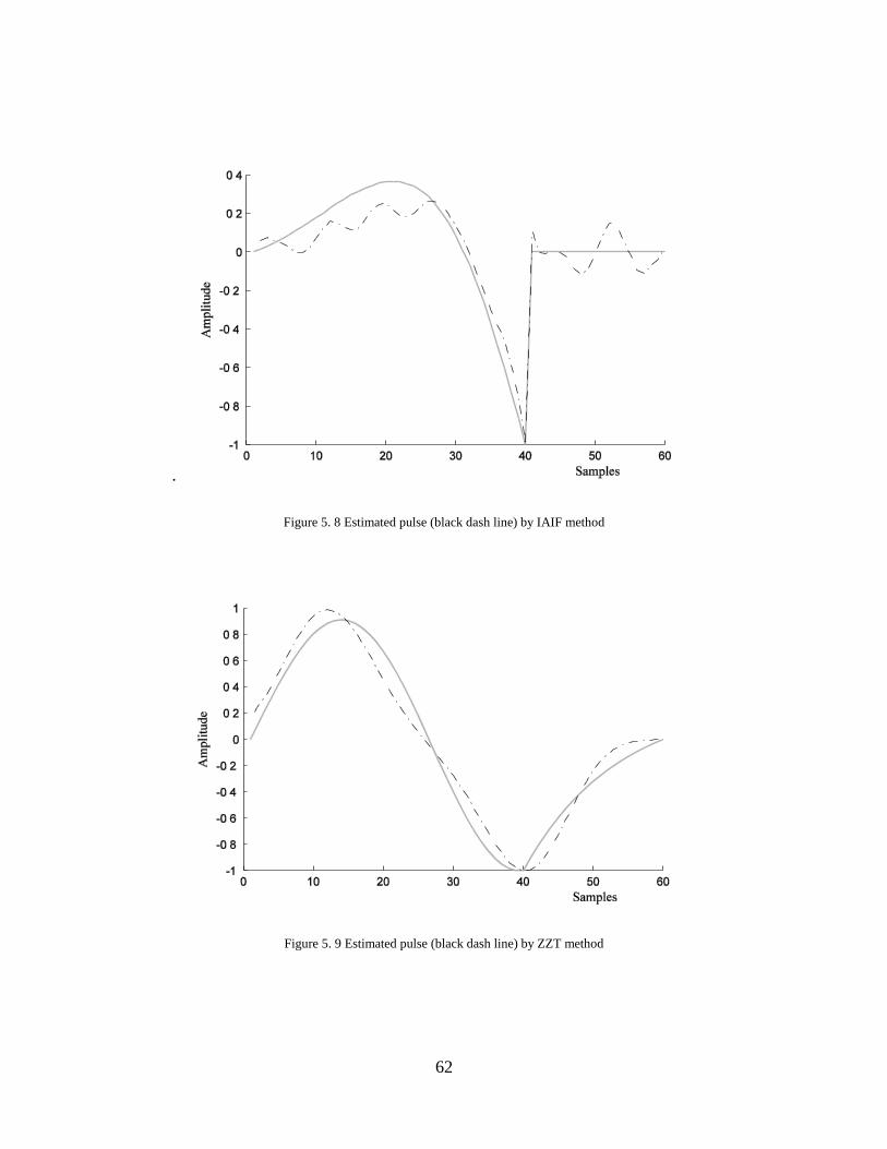
62

.

Figure 5. 8 Estimated pulse (black dash line) by IAIF method

Figure 5. 9 Estimated pulse (black dash line) by ZZT method

63

The ZZT method that separates maximum-phase from minimum-phase of speech

signal has an inferior estimation and resulting fitting results in Figure 5.9 comparing with

its counterpart in Figure 5.7(b) and Figure 5.8.

Although methods like LP+CC and IAIF have noticeable distortion when used to

recover the information contained in the close-phase region of LF model, they still

recover valuable information inside the open-phase region. All LF shaping parameters

and their quantities associated with these three distinct excitation estimation methods are

listed in Table 5.2 with their sample estimated pulses truncated by the window with

length of the synthetic pulse positioned at .

Table 5.1 Comparison of parameters of synthetic and fitting excitation pulses from different methods

Based on the quantities summarized in Table 5.1, we conclude that the two

estimation methods involving LP analysis and inverse filtering (LP+CC and IAIF) have

an advantage over the ZZT method. The separation of vocal-tract and GFP information

based on phase separation can be used to improve the result. But this approach lacks

β

error/ Energy

(Percent)

Synthetic Pulse 1 32 0.095 0.69 N/A

Fitting Pulse

( LP+CC) 1.881 30.22 0.094 15.451 12.18

Fitting Pulse

( IAIF) 1.004 30.197 0.058 12.4346 16.64%

Fitting Pulse

( ZZT) 1 25.55 0.0037 0.0756 63.21

64

some accuracy while dealing with the LF synthetic model in this set of experiments. The

fidelity of the open-phase portion of the original excitation information can be largely

preserved by LP analysis and its inverse filtering. Thus, it becomes at least a practical

benefit to extract real speakers’ excitation pulses for vowels and voiced sounds as their

private physical features as described in chapter 7.

Summary

In this chapter, we presented an improved approach based on the jointly

parametric and nonparametric estimation for vowels. Unlike most existing conventional

LP applications, we formulated an odd-order all-pole model to cancel the formants from

the vocal-tract response by inverse filtering, the result of which gives a way for further

refinement in terms of GFPs because of the obtaining of rough pulses after LP analysis

and inverse filtering. The phase characteristics of GFP and vocal-tract responses enable

us to employ the CC as a phase-decomposition based method to split the maximum-phase

and minimum-phase components of the signal from each another. Thus, this gives us an

effective way to enhance the estimation results from LP analysis.

As we employ limited data for each shifted LP window and apply inverse filtering

to estimate individual glottal pulses represented by open, return and close phase, we can

easily cascade these estimated pulses together to form a train together with the

information of pitch length variation. Therefore, the estimation results can be further

developed synchronously to recover a pulse train. The high computation-cost closely

associated with the detection of GCIs to locate an adequate pitch for analysis in phase-

65

decomposition methods can be avoided. According to what we have achieved in this

chapter, we can evaluate the effectiveness of the proposed method for extracting features

of real speech for a number of speech processing applications. An example of these

applications will be introduced in chapter 7 as another approach to evaluate our method.

66

CHAPTER SIX

JOINTLY PARAMETRIC AND NONPARMETRIC ESTIMATION

METHODS OF GLOTTAL FLOW PULSES II

Covariance methods of LP analysis typically based on all-pole models

representing the human vocal tract once dominated the glottal pulse extraction task [17],

[18]. They adapt LS algorithms to find the parameters for their models given the model

type and the number of parameters. Model-based approaches must assume model types

and model orders as a priori information; however, a priori information is generally

unknown. Thus, there are always some inaccuracies in these model-base approaches.

As a single LF model [7] was found by polynomial analysis to have the glottal

pulse return phase being mixed-phase [10]. Some nonparametric methods [31], [32] have

been used for the decomposition between the maximum-phase and minimum-phase parts

of speech signals. The decomposition results proved helpful to perform the source-tract

separation. Also the introduction of LS residual errors as a result of LP analysis affects

the extraction. Both of these two concerns will be taken into accounts while we design a

further processing procedure.

Higher-order homomorphic filtering is able to deal with the phase decomposition

and the suppression of noise introduced by the LP analysis and its corresponding inverse

filtering upon the speech sequence. The bicepstrum expression can be used to separate

the maximum and minimum-phase components [74]. The cumulant and cepstrum are

based on higher-order statistical (HOS) methods which help suppress effects of additive

noise and whitening residual errors which are byproducts of inverse filtering by

coefficients of LP analysis.

67

We here design an odd-order all-pole predictor to implement the LP analysis. If

the vocal-tract is lossy, it is assumed to be minimum-phase and represented by inside-

unit-circle complex conjugate poles of an all-pole model. Therefore, any individual

glottal pulse will be represented by at least one real pole from the model. First, we can

get a rough representation after the inverse filtering was applied to the original observed

speech sequence. Then we can improve the inverse-filtering results by applying HOS

processing to perform phase decomposition. And the bicepstrum representation of coarse

pulses will largely help suppress the errors coming from LS estimation in LP covariance

analysis.

Brief Background on Higher-Order Statistics

The covariance method of LP analysis together with an optimization algorithm

results in lower residual error level than the autocorrelation method which is based on

second-order statistics. Also, the autocorrelation function used in the autocorrelation

method will eliminate all phase information. Fortunately, we can look beyond second-

order statistics with help of higher-order cumulants given by [75]

( )

( )

where ( ) is the moment generating function of random variable .

If the order of statistical analysis is increased enough to look beyond the domain

of correlation and its frequency counterpart, we are able to find the magnitude and phase

information without the assumption about models, the number of model parameters, and

linearities of the system. The third-order cumulants, bispectrum and bicepstrum have

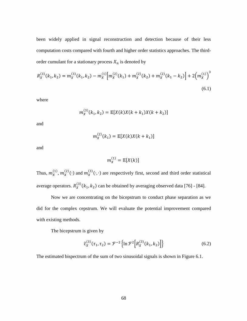
68

been widely applied in signal reconstruction and detection because of their less

computation costs compared with fourth and higher order statistics approaches. The third-

order cumulant for a stationary process is denoted by

( )( )

( )( ) ( )

[ ( )( )

( )( ) ( )( )] (

( ))

(6.1)

where

( )( ) ( ) ( ) ( )

and

( )( ) ( ) ( )

and

( )

( )

Thus, ( )

, ( )( ) and

( )( ) are respectively first, second and third order statistical

average operators. ( )( ) can be obtained by averaging observed data [76] - [84].

Now we are concentrating on the bicepstrum to conduct phase separation as we

did for the complex cepstrum. We will evaluate the potential improvement compared

with existing methods.

The bicepstrum is given by

( )( ) { [

( )( )]} (6.2)

The estimated bispectrum of the sum of two sinusoidal signals is shown in Figure 6.1.

69

Figure 6.1 Illustration of bispectrum of

Odd-Order Linear Prediction

Consider a speech signal , for which the -transform is denoted by

( ) ( ) ( ) (6.3)

Equation (6.3) represents the response of GFPs and the lip radiation modeled by the first-

order difference equation, and ( ) is the response of vocal tract that is a minimum-

phase system [25], which might contain zeros. ( ) can be represented by

70

( ) ( ) ( )

( ) ( ) ( )

where ( ) denotes all-zero part and ( ) denotes all-pole part of vocal-tract

response. The estimate of ( ) and ( ) leads to the source-tract separation.

Covariance methods of LP analysis, usually with even order, have become a

major tool for the parametric analysis of voiced speech utterances [17], [18] since they

can represent resonance frequencies characterizing the speaker’s vocal tract. On the other

hand, an odd-order all-pole model expressed by

( )

∑

guarantees that at least one real pole represents the low-pass tilting effect of the glottal

source. Then we can separate ( ) into two systems ( ) contributed by

complex pole pairs and ( ) contributed by real poles.

( ) ( ) ( ) (6.4)

holds after inverse filtering with ( ) obtained from LP analysis applied to ( ). Here

↔ ( ) and denotes the vector of LP residual errors.

Let [ ( )

( )

]

be a windowed discrete-time speech frame and

be the optimum estimate of in LS sense, then the all-pole model

coefficients vector [ ( )

( )

]

is found to minimize the norm error

between the observed signal and its estimation . In general,

‖ ‖

71

where ( ) is a data matrix shown in (5.3) and can be determined by

recursive LS algorithms.

Given a predictor coefficient vector with an odd number of elements, there

exists at least one real root , such that

( ) ∑

as the result of LS estimation. Then the remaining complex poles from excluding

are reserved for the representation of the coarse vocal-tract response, here is the set of

all roots of the above polynomial.

These estimated complex conjugate poles form a linear filter to deconvolve the

observed speech signal to obtain the coarse representation of the glottal source

corresponding to the current windowed speech frame. This leads to the estimated glottal

excitation ↔ ( ) expressed by

( ) ( )

( ) ( ) ( ) (6.5)

where ( ), the estimation of ( ), might contain some components from

the resonances ( ) of the speaker’s vocal tract.

In next step, we need to refine the glottal source estimates by removing those

remaining components of the vocal-tract response after the LP analysis and inverse

filtering. Meanwhile, how to suppress LS residual errors ( ) and the additive noise is

another concern in our approach.

72

High-Order Homomorphic Filtering

Rough results from the odd-order LP analysis and inverse filtering form a good

beginning for synchronized processing since the glottal closure instants becomes obvious.

From the phase characteristics of glottal source and vocal-tract responses, the phase

decomposition could be effective [31], [32] for dealing with the results from inverse

filtering, in which complex conjugate poles play an important role to cancel formants in

speech. HOS methods can be invoked to suppress the residual errors which are akin to

white noise. Based on the bicepstrum from the third-order cumulants of the current

speech sequence frame, we are able to achieve the refinement of individual glottal flow

pulses.

Consider a finite-length segment spanning slightly larger than one pitch period

within the estimated glottal source in Figure 6.1, and let ( )( ) denote the third-

cumulant in Figure 6.2 from an indirect estimator [85]. Notice the tilting effect due to the

bias [21].

Figure 6.2 Analysis region after LP analysis

73

Figure 6.3 The 3rd-order cumulant of the finite-length sequence

From (6.5), a linear convolution relation holds

(6.6)

where denotes the impulse response of the estimated glottal source corresponding to

the real pole or poles of ( ) in (6.5), and denotes estimated excitation.

Applying the two-dimensional -transfrom to ( )( ), we obtain

( )( ) {

( )( )}

to suppress additive noise where ( )( ) is the bispectrum of . If the residual error

response is assumed to have white noise-like properties between two successive

impulses, then from Appendix A, we have the bicepstrum ( )( ) corresponding to

the random output of linear system ( ) shown below

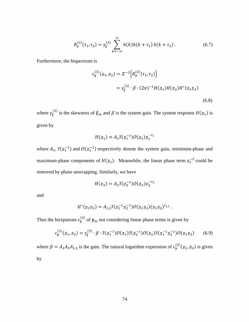
74

( )( )

( )∑ ( ) ( )

( ) (6.7)

Furthermore, the bispectrum is

( )( ) {

( )( )}

( )

( ) ( ) ( ) ( )

(6.8)

where ( )

is the skewness of and is the system gain. The system response ( ) is

given by

( ) ( ) ( )

where , ( ) and (

) respectively denote the system gain, minimum-phase and

maximum-phase components of ( ). Meanwhile, the linear phase term could be

removed by phase unwrapping. Similarly, we have

( ) ( ) ( )

and

( ) (

) ( )( )

Thus the bicepstrum ( )

of not considering linear phase terms is given by

( )( )

( ) (

) ( ) ( ) ( ) (

) ( ) (6.9)

where is the gain. The natural logarithm expression of ( )( ) is given

by

75

( )( ) |

( ) | (

) ( ) (

)

( ) ( ) ( ) (6.10)

The bicepstrum ( )( ) in the two-dimensional plane after taking inverse

transform of ( )( ) is given by [74]

( )( ) {

( )( )}

{

|

( ) |

( )

( )

( )

( )

( )

( )

(6.11)

All bicepstrum quantities except those at the origin along the axis can be

expressed as

( )

( ) {

− ( )

− ( )

(6.12)

where ( ) and ( )as differential cepstrum [85] terms are mapped to the bicepstrum

plane to derive the complex cepstrum ( ) with the property [74], [87]

76

( )( ) ( )

Since maximum-phase components ( )( ) and minimum-phase components

( )( )

lie in the left and right hand of origin of cepstrum plane, we can recover both maximum-

phase and minimum-phase impulse response by applying an operator − to

( )( ) and

( )( ). Here − is the reverse transform of where

( ). Then the maximum-phase component can be reserved as a refined GFP [19].

However, we need to consider linear phase terms in (6.10) and corresponding

effects from those. Note that two-dimensional phase unwrappings to overcome phase

discontinuities before applying the natural logarithm to the bispectrum will be much

harder than what we did to calculate the cepstrum in one-dimensional case. We can

circumvent the two-dimensional phase unwrapping by utilizing the relation [74], [85]

( )

( ) [ ( )

( )] ( )

( ) (6.13)

where “ ” denotes two-dimensional convolution operator. A set of cepstral equations

derived from above expression are listed in [85] as

∑ ( )[ ( )( )

( )( )]

∑ ( )[ ( )( )

( )( )]

( )( )

(6.14)

where and are parameters to restrict the numbers of coefficients ( ) , ( ) and

, .

77

Simulation Results

In order to evaluate the performance of the proposed approach of estimating

individual GFPs, two sets of experiments were performed. A sampling rate of 8kHz was

used.

An estimation of a GFP from a real vowel from a male speaker is shown in

Figure 6.4. The pulse which results from the inverse filtering in Figure 6.2 behaves as an

input to a conventional indirect estimator [84] for the third-order cumulant with

and after comparing different combinations of and values [86], [87].

Figure 6.4 Normalized GFP estimation from a real vowel /a/

Another single pulse is generated in Figure 6.5(a) by convolution of two

exponential sequences [39].

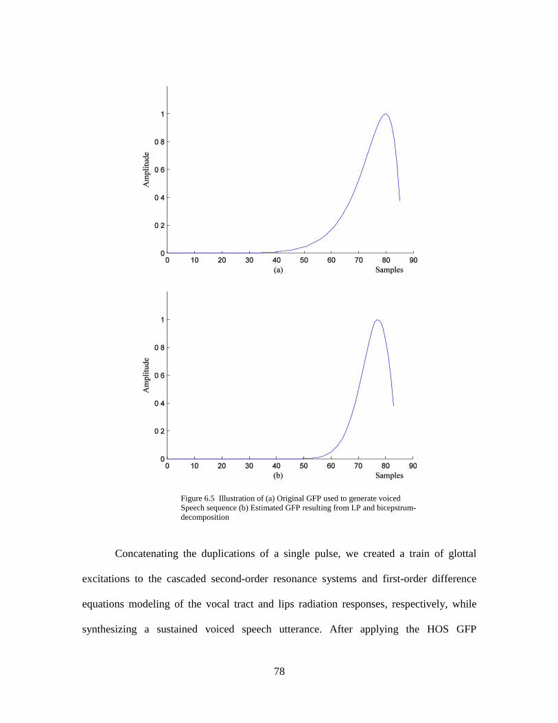
78

Figure 6.5 Illustration of (a) Original GFP used to generate voiced

Speech sequence (b) Estimated GFP resulting from LP and bicepstrum-

decomposition

Concatenating the duplications of a single pulse, we created a train of glottal

excitations to the cascaded second-order resonance systems and first-order difference

equations modeling of the vocal tract and lips radiation responses, respectively, while

synthesizing a sustained voiced speech utterance. After applying the HOS GFP

79

estimation approach, we can recover the excitation signal, especially, individual pulses.

The process can be summarized by Figure 6.6.

Figure 6.6 Workflow to recover exciting synthetic glottal pulse

A comparison can be made through the single pulse estimation shown in Figure

6.5(b) as the result of 12-pole inverse filtering and HOS homomorphic filtering of one

segment of observed data. Notice that the estimated GFP shown in Figure 6.5(b) has a

steeper decreasing attenuation than that of in Figure 6.4(a) in its open-phase portions.

This distortion is normally introduced by insufficient samples while calculating the

average [88]. The waveform shown in Fig. 6.5(b) is free of whitening residue errors since

they were suppressed by the bicepsturm method already described. The bicepstrum

quantities along the axis axis are obtained, while the origin is discarded.

A quantitative comparison was calculated of parameter sets between the synthetic

pulse and fitted waveform to analyze the performance of the estimation methods based on

our observations of data excited by cascaded synthetic LF models with those known

parameters.

GFP

Estimation

Vocal-tract

Model Lips

Radiation

Synthetic LF

model Recovered

Pulses

80

Figure 6.7 (a) Synthetic LF excitation pulse (b) Estimated pulse (black dash line)

and fitted pulse (gray solid line)

81

Table 6.1 Comparison of parameters of synthetic and fitted excitation pulses

The peak value of overshoot of the estimated pulse in the open phase in Figure 6.7

(b) exceeds that of the pulse shown in Figure 6.7(a). Also, the values of the parameter

and for the synthetic pulse differ from those of the fitted pulses. These three

parameters and β determine the shape of fitted pulse in open phase. See Table 6.1.

The overall fitting error implies that it has better performance than the pure phase

separation method with the LF model used to represent the excitation pulse. Several

papers [84], [89] mentioned that higher-order statistics are immune to Gaussian noises.

The distortions shown in Figure 5.6(b) can be suppressed.

Summary

In this chapter, we presented a technique combining LP and HOS processing to

estimate and model the GFP waveform for voiced speech sounds. The return-phase

information can be estimated and the residue errors from LP analysis due to the inverse

filtering after LP covariance analysis can be suppressed. A large computation cost of

accurate GCI detections [9] can be avoided if the inverse filtering is applied to find

β

error/ Energy

(Percent)

Synthetic Pulse 1 32 0.095 0.69 N/A

Fitting Pulse 16.6 16.8 0.0177 0.144 35.54%

82

coarse estimation of GFPs with the reciprocal of complex conjugate poles from an all-

pole LP model. However, the lack of prior information while setting parameter and

might bring distortions to estimated pulses.

83

CHAPTER SEVEN

A SMALL SCALE SPEAKER IDENTIFIER WITH LIMITED

EXCITING INFORMATION

As glottal pulses had been intuitively to consider containing excitation

information from a specific speaker, the estimated glottal pulse in chapter 5 gives us a

direct representation of the continuous information as pulses in waveform. Extracting

parameter values from the continuous information to form speaker’s features, we can try

to apply these new feature values to training models for speaker recognition. Followed by

a maximum and minimum phase separation operation, the glottal pulses are estimated

using linear prediction followed by its inverse filtering by estimated LP all-pole

coefficients. These estimated waveforms can be fitted by a new LF glottal flow derivative

model whose shape can be adjusted through its parameters to minimize the least-square

errors between target waveform and fitting model as previously described in chapter 5.

Estimating these LF model parameters obtained from the inverse filtering of

linear prediction applying to the original speech, and complex cepstrum coefficients, we

set up a training set for each speaker who was used as a test subject later on in the

realization of a speaker identification system. Then a classification system based on

minimum distance rule is applied to testing data for each subject to decide which centroid

is nearest to the current testing subject among all centroids in the sense of least

Minkowski-distance or by other metrics. Then labels corresponding to centroids can be

assigned to all observed testing features in this way. The identifiability of speech features

in terms of estimated glottal flow pulses of all subjects is thus determined as a result of

the experiment.

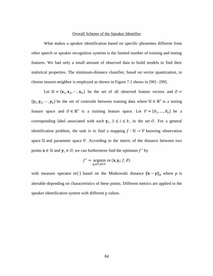
84

Overall Scheme of the Speaker Identifier

What makes a speaker identification based on specific phonemes different from

other speech or speaker recognition systems is the limited number of training and testing

features. We had only a small amount of observed data to build models to find their

statistical properties. The minimum-distance classifier, based on vector quantization, to

choose nearest neighbor is employed as shown in Figure 7.1 shows in [90] - [99].

Let { } be the set of all observed feature vectors and

{ } be the set of centroids between training data where is a testing

feature space and is a training feature space. Let { } be a

corresponding label associated with each , , in the set . For a general

identification problem, the task is to find a mapping knowing observation

space and parameter space . According to the metric of the distance between two

points and , we can furthermore find the optimum by

( )

with measure operator ( ) based on the Minkowski distance ‖ ‖ where is

alterable depending on characteristics of these points. Different metrics are applied to the

speaker identification system with different p values.

85

OBJECTIVE MODELS

Feature Identified

Figure 7.1 Speaker identification system to choose models

Figure 7.2 Decision boundaries for centroids based on Minimum Euclidean Distance

.

.

.

Speaker

Select

Models With

Minimum

Distance

Speaker 𝑘

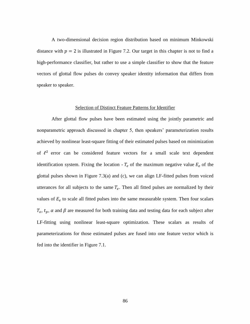
86

A two-dimensional decision region distribution based on minimum Minkowski

distance with is illustrated in Figure 7.2. Our target in this chapter is not to find a

high-performance classifier, but rather to use a simple classifier to show that the feature

vectors of glottal flow pulses do convey speaker identity information that differs from

speaker to speaker.

Selection of Distinct Feature Patterns for Identifier

After glottal flow pulses have been estimated using the jointly parametric and

nonparametric approach discussed in chapter 5, then speakers’ parameterization results

achieved by nonlinear least-square fitting of their estimated pulses based on minimization

of error can be considered feature vectors for a small scale text dependent

identification system. Fixing the location - of the maximum negative value of the

glottal pulses shown in Figure 7.3(a) and (c), we can align LF-fitted pulses from voiced

utterances for all subjects to the same . Then all fitted pulses are normalized by their

values of to scale all fitted pulses into the same measurable system. Then four scalars

, , and are measured for both training data and testing data for each subject after

LF-fitting using nonlinear least-square optimization. These scalars as results of

parameterizations for those estimated pulses are fused into one feature vector which is

fed into the identifier in Figure 7.1.

87

Figure 7.3 Illustrations of a single estimated glottal flow derivatives and their

fitting pulses. (a) Estimated pulse for Speaker A (b) LF-fitting pulse with estimate

parameters: , , , (c) Estimated pulse

for Speaker B (d) LF-fitting pulse with estimate parameters: , ,

,

88

The difference vector between a testing feature pattern and each training

centroid can be easily obtained by | | where an element

( )

| ( ) ( )

|. A deviation ratio vector between the current testing vector and all

centroids will be scaled by applying the Kronecker product of between and

which is vector of reciprocals of the elements of centroid . Furthermore, the class label

will be decided based on the minimum norm on between the current

testing pattern and the th centroid .

The parameters shown in Figure 7.3 come from the optimum coefficients of

Trust-Region fitting with the LF model (3.3) based on estimated pulses for a real speech

voiced phoneme for the limited speaker population involved in the experiment. These LF

model parameters , , and or other ones used for the geometrical representation of

a class of waveforms will increasingly reduce the distance among distinct patterns if the

body of subjects is expanded. Meanwhile, the fitting task, which is in fact an

approximation to the observed function or sequence, will automatically remove some

valuable information that probably contained in the estimation of glottal flow pulses or

derivatives. Therefore, these two weaknesses closely associated with fitting parameters as

feature patterns of speakers will increase the challenge of performing discrimination

when more subjects are included in the tests.

Some existing mature identification systems [100] – [106] employing cepstrum

coefficients or a variety of frequency coefficients as speaker features have demonstrated

good performance. If any method of estimating information about glottal pulses is

89

effective, it should be possible to use this information to improve the overall

identification performance.

A brief summary of a speaker-identification system based on complex cepstrum

performance is now given. A group of complex cepstrum quantities ( ) for each pulse

within one-pitch interval, generated by the windowed all-pole LP analysis and

corresponding inverse filtering with those estimated coefficients for the LP model, are

used to investigate whether excitation information of a speaker is contained in the

estimated representation of complex cepstrum. Because ( ) ( ) ( )

where ( ) and ( ) denote cepstrum quantities in terms of maximum-phase and

minimum-phase components [23], we can apply linear liftering to split ( ) and

( ) as what we did in chapter 5.

Complex cepstrum quantities corresponding to maximum-phase components of

the estimated pulse after LP analysis and inverse filtering are therefore collected as

feature vectors for the current speaker. As cepstrum quantities related to maximum-phase

components mainly comes from LF model excitation source [13], [19], the

representations of these components, with negative index in cepstrum frequency domain,

can be used to formulate features for all subjects involved in the identifier. To check

whether the glottal flow pulses carry information which can be used to help identify

distinct subjects, training and testing features coming from estimated pulses for each

subject are applied to the identifier in Figure 7.1.

90

Additionally, the complex cepstrum coefficients for a single glottal flow pulse for

each term of two distinct speakers and the extracted portion to form feature vectors for

these two speakers are shown in Figure 7.4.

Figure 7.4 Illustrations of complex cepstrum coefficients of a single estimated

glottal flow pulse and extraction of low cepstrum-frequency quantities. (a) complex

cepstrum coefficients for Speaker A (b) quantities used for feature pattern

about speaker A (c) complex cepstrum coefficients for Speaker B (d) quantities

used for feature pattern about Speaker B

91

With glottal flow pulses estimated with the jointly parametric and nonparametric

approach, 13 complex-cepstrum coefficient vectors corresponding to maximum-

phase components for all speakers’ were collected to form both training space and

testing space as what we did when using LF fitting parameters. Difference vector

between a testing feature pattern and each training centroid can be obtained by

| | as for LF model feature vectors. Furthermore, the class parameter

will be decided based on the minimum Euclidean distance, ‖ ‖

, between the current

testing pattern and the th centroid . With 8 kHz sampled testing and training

utterances of vowel from 12 distinct subjects, the identification performance for

features from the LF-model and complex cepstrum coefficients corresponding to

maximum-phase are summarized in Table 7.1.

Features Correctness - %

LF-model parameters 83.3

CC parameters 75.0

Table 7.1 Speaker identification results for two different features

Inconsistent modes of phonation in terms of each subject: normal, pressed or

breathy, could result in variations of estimated excitation waveforms even for the same

speaker. This introduces variations and sensitivities to feature patterns used in the

identifier. Thus, an identifier which employs only excitation information might be very

inadequate without other speech information, especially with a large number of subjects.

92

However, combining features from the LF model with other speech features such as pitch

or vocal-tract response will be expected to enhance speaker recognition system based on

only one of these two feature sets.

93

CHAPTER EIGHT

CONCLUSIONS

This dissertation has investigated human speech production, source-tract

interaction mechanisms and a variety of proposed glottal models that are central to the

problem of estimating the periodic glottal excitation for voiced sounds or vowels.

Although there exist some estimation schemes and some progress in the area of

recovering the excitation information, they were restricted by some negative factors like

strict assumptions and high computational complexities. Based on concerns about these

limitations, we proposed two jointly parametric and nonparametric excitation estimation

approaches, which employ phase decomposition without any assumed model type and

just one step of LP analysis and inverse filtering for each flexible sliding window, to

improve estimation results by using LP inverse filtering and homomorphic processing.

Estimated glottal pulse parameters were evaluated for their effectiveness for a speaker

identification using LF fitting model parameters and complex cepstrum coefficients as

features. These features are used to estimate a speaker’s glottal characteristics as voiced

phonemes are pronounced.

Jointly Parametric and Nonparametric Excitation Estimation

For Real and Synthetic Speech

Recovering the excitation signal of a voiced speech utterance is in fact an inverse

problem where the source cannot be observed directly. This fact adds complexities to the

evaluation of estimation results. The speech signal results from interactions of glottal

94

excitation, vocal-tract response and lips radiation. Linear system theory provides a

theoretical basis for estimating the glottal excitations as is proposed in this dissertation.

Different aspects of glottal excitation and vocal tract together with their combinational

effects have been employed, including least-squares inverse filtering, IAIF, ZZT and CC.

Each approach has its own advantages and restrictions. Our ultimate research goal was to

discover new strategies to employ their advantages and minimize their weaknesses in a

way to extract the glottal source information from speech utterances for voiced phonemes

and to suppress the response of vocal tract in the process of recovering glottal source

waveforms. Linear prediction and phase separation as two mature tools in speech analysis

were combined to produce an enhancement to generate a smooth glottal pulse curve as

shown in chapter 5. With the efficient use of frame-by-frame, odd-order LP analysis and

its corresponding inverse filtering, the response of excitations from a speaker can be

recovered. Multiple inverse filtering sections in IAIF [4] are no longer necessary in the

process of recovering excitation information. Also, the accurate detection of glottal

closure instants to fix two ending points of the analysis region for the following phase

separation section to split maximum-phase components from minimum-phase

components is also no longer necessary. Additionally, our method of frame-by-frame LP

analysis and inverse filtering saves computation costs without precise detection of

glottal closure instants and largely increases the robustness of the detection of these

points in phase-separation.

Another approach employing third-order cummulants and the bicepstrum to refine

the glottal waveform estimated from the previous LP analysis and inverse filtering was

95

thoroughly described in chapter 6. The third-order cumulants and the bicepstrum can

largely reject the distortions because of mismatch in the process of cancelling vocal-tract

effects due to inverse filtering. The estimated pulses were smooth and free of noises after

the LP inverse filtering.

Two different evaluation schemes were used to evaluate the validity of the

estimated pulses. Firstly, these two jointly parametric and nonparametric approaches

were applied to a real vowel utterance from human speech and the results of estimating

the glottal pulse were presented. Secondly, two synthetic pulses produced by different

generation methods (1) convolution of two exponential sequences [39] and (2) using the

LF model, are used to synthesize pulse trains to excite an artificial vocal-tract model

represented by complex pole pairs, to generate a synthetic voiced speech utterance. The

glottal pulse estimation method was applied to the synthetic utterance generated by the

first method was directly compared with the synthetic pulse. And the estimation based

on the utterance generated by the second method was be nonlinearly fitted by an LF

model whose shape can be adjusted by several parameters [9]. These fitted parameters

were further compared with those parameters used to synthesize LF-modeling pulses

originally. Then the performance of the jointly parametric and nonparametric approaches

was evaluated in terms of distinct types of synthetic excitation pulses as described above.

Features from Estimated Glottal Pulses for Speaker Identifier

The LF-fitted parameterization of estimated pulses for a speaker provides a

feature vector as excitation information for him. The complex cepstrum quantities

96

corresponding to maximum-phase components were also clustered as feature vectors for

different speakers. For either type of feature vectors, a small scale text-dependent speaker

identification system was implemented. This system was based on the minimum-distance

decision between the observed feature and centroids for all speakers. Although the

population involved was small, the speaker identification experiments showed that glottal

excitation parameters estimated by the proposed method performed better than complex

cepstrum parameters obtained from the same data.

Suggested Directions of Research

The field of extraction of glottal source information is young and full of

challenges. All speech processing domains that potentially employ bioinformatics could

benefit from the addition of this type of information.

The problem of separating glottal source from vocal-tract information still

presents challenges. The solution to this inverse problem will largely depend on new

experimental and theoretical discoveries about interaction between source and vocal-tract

components. With the help of these physical and theoretical explorations, better

understanding of the roles played by both glottal pulses and vocal tract in the generation

of voiced utterances will help researchers apply this knowledge to a variety of speech

processing applications. Features which are byproducts of pulse estimation, along with

maximum-phase cepstrum coefficients and other features from speakers, may be applied

to speaker indentification with larger populations. The development of a robust speaker

97

identification system that can perform well in a degraded environment, like in telephone

speech, should also benefit from the methods proposed in this dissertation.

98

APPENDICES

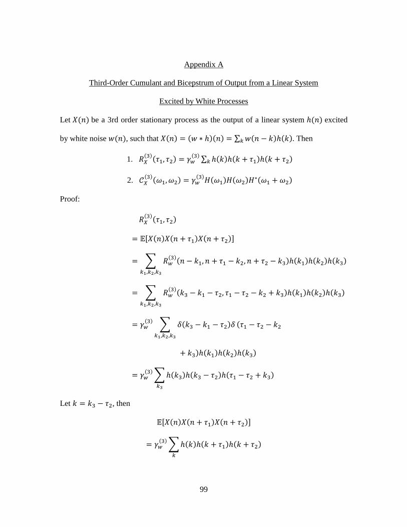
99

Appendix A

Third-Order Cumulant and Bicepstrum of Output from a Linear System

Excited by White Processes

Let ( ) be a 3rd order stationary process as the output of a linear system ( ) excited

by white noise ( ), such that ( ) ( )( ) ∑ ( ) ( ) . Then

1. ( )( )

( ) ∑ ( ) ( ) ( )

2. ( )( )

( ) ( ) ( )

( )

Proof:

( )( )

( ) ( ) ( )

∑ ( )( ) ( ) ( ) ( )

∑ ( )( ) ( ) ( ) ( )

( )

∑ ( )

(

) ( ) ( ) ( )

( )

∑ ( ) ( ) ( )

Let , then

( ) ( ) ( )

( )

∑ ( ) ( ) ( )

100

Here, the proof of the 1st part is completed.Now we express the bispectrum

( )( )

in terms of ( )( ) . Let

( )( ) ( )(

) by setting and . Then

( )( )

( )( ) ∑ ( )( ) ( ) ( ) ( )

So

( )( ) ∑ ∑

( )( ) ( )

after arrangements,

( )( ) ∑ ( ) ( ) ( ) (∑

( )(

) ( ))

Substitute

∑ ( )( )

( )

( ) ( ) ( )

into ( )( ), we get

( ) ∑ ( ) ( ) ( ) ( )

( ) ( )

Since ( ) ( )

for statistical independent process, the above expression

becomes

∑ ( ) ( ) ( )

( )

101

Thus ( )( )

( ) ( ) ( )

( ). The proof is completed.

102

REFERENCES

[1] G. Fant. Acoustic theory of speech production. Mouton, The Hague, The

Netherlands. 1960.

[2] R. Miller. Nature of the vocal cord wave. Journal of the Acoustical Society of

America, 31: 667–677, 1959.

[3] M. Matausek and V. Batalov. A new approach to the determination of the glottal

waveform. IEEE Transactions on Acoustics, Speech and Signal Processing,

28:616-622, Dec. 1980.

[4] P. Alku. Glottal wave analysis with pitch synchronous iterative adaptive inverse

filtering. Speech Communication, 11(2):109–118, 1992.

[5] P. Alku. An automatic method to estimate the time-based parameters of the glottal

pulseform. Proceeding of IEEE International Conference on Acoustics, Speech,

and Signal Processing, 2:29-32, 1992.

[6] A. Rosenberg. Effect of glottal pulse shape on the quality of natural vowels.

Journal of the Acoustical Society of America, 49(2B):583–590, 1971.

[7] J. Deller, J. Hansen and J. Proakis. Discrete-time processing of speech signals,

New York, Wiley-IEEE Press. 1999.

[8] T. Raitio, A. Suni, J. Yamagishi, H. Pulakka, J. Nurminen, M. Vainio and P. Alku.

HMM-based speech synthesis utilizing glottal inverse filtering. IEEE

Transactions on Audio, Speech & Language Processing, 19(1): 153-165, 2011

[9] D. Klatt and L. Klatt. Analysis, synthesis, and perception of voice quality

variations among female and male talkers. Journal of the Acoustical Society of

America, 87(2):820–857, 1990.

[10] G. Fant, J. Liljencrants, and Q.-G. Lin. A four-parameter model of glottal flow.

STL-QPSR, 26(4):1–13, 1985.

[11] M. Plumpe, T. Quatieri and D. Reynolds. Modeling of the glottal flow derivative

waveform with application to speaker identification. IEEE Transactions on

Speech and Audio Processing, 7(5):569–586, Sep. 1999.

[12] G. Fant. The LF-model revisited. Transformations and frequency domain

analysis. STL-QPSR, 36(2-3):119–156, 1995.

103

[13] B. Doval, C. d’Alessandro, and N. Henrich. The voice source as a

causal/anticausal linear filter. Proceeding of ISCA Voice Quality: Functions,

Analysis and Synthesis (VOQUAL), 16–20, 2003.

[14] J. Flanagan. Note on the design of “terminal-analog” speech synthesizers. Journal

of the Acoustical Society of America, 29:306–310, 1957b.

[15] J. Flanagan. Some properties of the glottal sound source. Journal of Speech and

Hearing Research, 1:99–116, 1958.

[16] W. Mason. The approximate networks of acoustic filters. Journal of the

Acoustical Society of America, 1(2A): 263-272, 1930.

[17] I. Lim and B. Lee. Lossless pole-zero modeling of speech signals. IEEE

Transactions on Speech and Audio Processing, 1(3):269–276, Jul. 1993.

[18] L. Rabiner and R. Schafer. Digital processing of speech signals. Englewood

Cliffs, Prentice Hall, 1978.

[19] B. Bozkurt, B. Doval, C. D’Alessandro and T. Dutoit. Zeros of Z-transform

representation with application to source-filter separation in speech. IEEE Signal

Processing Letters, 12(4):344–347, Apr. 2005.

[20] J. Deller. On the time domain properties of the two-pole model of the glottal

waveform and implications for LPC. Speech Communication: An

Interdisciplinary Journal, 2:57–63, 1983.

[21] D. Y. Wang, J. D. Markel and A.H. Gray. Least squares glottal inverse filtering

from the acoustic speech waveform. IEEE Transactions on Acoustics, Speech,

And Signal Processing, ASSP-27(4):350–355, Aug. 1979.

[22] K. Funaki, Y. Miyanaga and K. Tochinai. Recursive ARMAX speech analysis

based on a glottal source model with phase compensation. Signal Processing,

74:279–295, 1999.

[23] A. Oppenheim. Discrete-Time Signal Processing. 3rd ed., Upper Saddle River,

Prentice Hall. 2009.

[24] J. Demmel. Applied Numerical Linear Algebra, SIAM. Aug. 1997.

[25] D. Manolakis, V. Ingle and S. Kogon. Statistical and adaptive signal processing:

spectral estimation, signal modeling, adaptive filtering and array processing.

Artech House Signal Processing Library. 2005.

104

[26] J. Proakis, C. Rader, F. Lin, M. Moonen, I. Proudler, C. Nikias. Algorithms for

statistical signal processing. Prentice Hall, 2002.

[27] A. Yeredor. The extended least squares criterion: minimization algorithms and

application. IEEE Transactions on Signal Processing. 49(1):74–86, Jan. 2000.

[28] D. Feng, Z. Bao and L. Jiao. Total least mean squares algorithm. IEEE

Transactions on Signal Processing. 46(8):2122–2130, Aug. 1998.

[29] S. Chandra and L. Wen. Experimental comparison between stationary and

nonstationary formulations of linear prediction applied to voiced speech analysis.

IEEE Transactions on Signal Processing. 22(6):403–415, 1974.

[30] P. Murthy and B. Yegananarayana. Robustness of group-delay-based method for

extraction of significant instants of excitation from speech signals, IEEE

Transactions on Speech and Audio Processing. 7(6):609–619, Nov. 1999.

[31] P. Naylor, A. Kounoudes, J. Gudnason, and M. Brookes. Estimation of glottal

closure instants in voiced speech using the DYPSA algorithm. IEEE Transactions

on Speech Audio Processing. 15(1):34–43, Jan. 2007.

[32] R. Smits and B. Yegnanarayana. Determination of instants of significant

excitation in speech using group delay function. IEEE Transactions on Speech

and Audio Processing. 3(5):325-333, Sep. 1995.

[33] M. Thomas and P. Naylor. The sigma algorithm: A glottal activity detector for

electroglottographic signals. IEEE Transactions on Audio, Speech, and Lang.

Processing. 17(8):1557–1566, Nov. 2009.

[34] E. Abberton, D. Howard, and A. Fourcin. Laryngographic assessment of normal

voice: A tutorial. Clinical Linguist. Phon., 3:281–296, 1989.

[35] T. Drugman, B. Bozkurt and T. Dutoit. Complex cepstrum-based decomposition

of speech for glottal source estimation. Proceedings of Interspeech, 2009.

[36] J. Makhoul. Linear prediction: A tutorial review. Proceedings of the IEEE,

63:561–580, Apr. 1975.

[37] T. Tremain. The government standard linear predictive coding algorithm: LPC-

10. Speech Technology, 1:40–49, Apr. 1982.

[38] T. Drugman, B. Bozkurt and T. Dutoit. Causal–anticausal decomposition of

speech using complex cepstrum for glottal source estimation. Speech

Communication. 53(6):740–741, Jul. 2011.

105

[39] T. Quatieri. Discrete-Time Speech Signal Processing. Upper Saddle River,

Prentice Hall. 2001.

[40] R. Schaback. Convergence analysis of the general Gauss-Newton method.

Numerische Mathematik, 46:281-309, 1985.

[41] L. Lasdon and A. Waren. Survey of Nonlinear Programming Applications.

Operations Research. 28(5):1029–1073, 1980

[42] N. Jorge and J. Stephen. Numerical Optimization. 2nd ed., Springer. Jul. 2006

[43] C. Kelley. Iterative Methods for Optimization. SIAM Frontiers in Applied

Mathematics, 18, 1999

[44] T. Strutz. Data Fitting and Uncertainty: A practical introduction to weighted least

squares and beyond. Vieweg and Teubner. Nov. 2010

[45] S. Gratton. A. Lawless and N. Nichols. Approximate Gauss-Newton methods for

nonlinear least squares problems. SIAM Journal on Optimization, 18(1), Feb.

2007

[46] D. Bates and D. Watts. Nonlinear Regression and Its Applications. New York:

Wiley, 1988.

[47] D. Gorinevsky. An approach to parametric nonlinear least square optimization

and application to task-level learning control. IEEE Transactions on Automatic

Control, 42(7):912–927, Jul. 1997

[48] J. Dennis, D. Gay and R. Welsch. An adaptive nonlinear least-squares algorithm.

ACM Transactions on Mathematical Software, 7:348–368, Sept. 1981.

[49] K. Levenberg. A method for the solution of certain problems in least squares.

Quarterly of Applied Mathematics, 2:164–168, 1944.

[50] D. Marquardt. An Algorithm for Least-Squares Estimation of nonlinear

parameters. Journal of the Society for Industrial and Applied Mathematics,

11(2):431–441, 1963

106

[51] X. Luo, L. Liao and H. Tam. Convergence analysis of the Levenberg-Marquardt

method. Optimization Methods and Software, 22(4):659–678, Aug. 2007

[52] J. Dennis and L. Vincente. Trust-region interior-point algorithms for minimization

problems with simple bounds. SIAM Journal of Control and Optimization, TR94–

42, Nov, 1994

[53] T. Coleman and Y. Li. An interior trust region approach for nonlinear

minimization subject to bounds. SIAM Journal on Optimization, 6(2):418–445,

1996

[54] J. Dennis, M. Heinkenschloss and L. Vincente. Trust-Region Interior-Point SQP

Algorithms for a Class of Nonlinear Programming Problems. SIAM Journal of

Control and Optimization, 36(5):1750–1794, 1998

[55] R. Byrd, J. Gilbert and J. Nocedal. A Trust Region Method Based on Interior

Point Techniques for Nonlinear Programming. Mathematical Programming,

89(1):149–185, 2000.

[56] J. More. Recent developments in algorithms and software for trust-region

methods. In A. R. Bachem, M. Grotshel and B. Korte, Eds., Mathematical

Programming: The State of the Art, Springer-Verlag, Berlin, 258–287, 1983.

[57] Y. Yuan. On the convergence of trust region algorithm. Mathematica Numerica

Sinica, 16(3):333–346, 1996.

[58] A. Conn, N. I. Gould and P. Toint. Trust region methods. Philadelphia, MPS-

SIAM Series on Optimization, SIAM, 2000.

[59] F. Bastin, V. Malmedy, M. Mouffe, P. Toint and D. Tomanos. A retrospective

trust-region method for unconstrained optimization. Mathematical Programming,

123(2): 395–418, 2010.

[60] X. Zhang, Z. Chen and J. Zhang. A self-adaptive trust region method

unconstrained Optimization. Operations Research Transactions, 5(1):53–62,

2001.

[61] N. Karmarkar. A new polynomial time algorithm for linear programming.

Combinatorica, 4(4):373–395, 1984.

107

[62] S. Mehrotra. On the implementation of a primal-dual interior point method. SIAM

Journal on Optimization, 2(4): 575–601, 1992.

[63] F. Potra and S. Wright. Interior-point methods. Journal of Computational and

Applied Mathematics, 124:281–302, 2000.

[64] A. Forsgren, P. Gill and M. Wright. Interior methods for nonlinear optimization.

SIAM Rev.44, 525–597, 2002.

[65] F. Potra. Q-superlinear convergence of the iterates in primal-dual interior-point

methods. Math. Programming, 91(Ser.A):99–115, 2001.

[66] C. Kelley, Solving nonlinear equations with Newton's method. SIAM. 2003.

[67] W. Press, B. Flannery, S. Teukolsky and W. Vetterling. “General Curve Fit”,

Numerical Recipes in C. Cambridge University Press. 1988.

[68] W. Press, B. Flannery, S. Teukolsky and W. Vetterling. “Cubic Spline Curve Fit”,

Numerical Recipes in C. Cambridge University Press. 1988.

[69] J. Wolberg. Data analysis using the method of least squares: Extracting the most

information from experiments. 1st ed., Springer, Feb. 2006.

[70] S. Ahn. Least squares orthogonal distance fitting of curves and surfaces in space.

1st ed., Springer. Jan. 2005.

[71] H. Wang, Y. Ge, Z. Liu; H. Liu, L. Xu. One curve-fit method for the

evaluation of the total distortion of sinusoidal signal. Proceedings of IEEE

International Conference on Information and Automation (ICIA), 2010.

[72] P. Scott. Minimax and L1 curve fitting in non-Gaussian MAP estimation. IEEE

Transactions on Automatic Control, 20(5):690–691, 1975.

[73] N. Greggio, A. Bernardino, C. Laschi, P. Dario and J. Santos-Victor. An

Algorithm for the Least Square-Fitting of Ellipses. Proceedings of IEEE

International Conference on Tools with Artificial Intelligence (ICTAI), 351–353,

2010.

[74] A. Papoulis and S. Pillai. Probability, random variables and stochastic processes.

4th ed., McGraw-Hill. 2002.

108

[75] W. Collis, P. White and J. Hammond. High-order spectra: the bespectrum and

trispectrum. Mechanical Systems and Signal Processing, 12(3):375–394, May

1998.

[76] T. Hall and G. Giannakis. Bispectral Analysis and Model validation of Texture

Images. IEEE Transactions on Image Processing, 4(7):996–1009, Jul. 1995.

[77] Y. Wu and A. Leyman. Time delay estimation in unknown spatially correlated

Gaussion noises using higher-order statistics, Proceedings of IEEE International

Conference on Acoustics, Speech and Signal Processing, 2813–2816, 1999.

[78] D. Ruiz and A. Gallego. Bispectrum estimation using AR-modelling. The

International Journal for Computation and Mathematics in Electrical and

Electronic Engineering, 18(1):43–60, 1999.

[79] A. Petropulu, and C. Nikias. The complex cepstrum and bicepstrum: analytic

performance evaluation in the presence of Gaussian noise. IEEE Transactions on

Acoustics, Speech and Signal Processing, 38(7):1246–1256, Jul. 1990.

[80] P. Molchanov, J. Astola, K. Egiazarian and A. Totsky. Moving target

classification in ground surveillance radar ATR system by using novel bicepstral-

based information features. European Radar Conference (EuRAD), 194–197,

2011.

[81] Y. Zhou, Y. Liu, H. An and L. Che. Higher order spectral analysis for vibration

signals of the large steam turbine in slow-down process. Proceedings of IEEE

International Conference on Intelligent Control and Information Processing

(ICICIP), 1149–1154, 2011.

[82] H. Hsieh, H. Chang and M. Ku. Higher-order statistics based sequential spectrum

sensing for cognitive radio. Proceedings of IEEE International Conference on ITS

Telecommunications (ITST), 696–701, Aug. 2011.

[83] P. Shih and D. Chang. An automatic modulation classification technique using

high-order statistics for multipath fading channels. Proceedings of IEEE

International Conference on ITS Telecommunications (ITST), 691–695, Aug.

2011.

[84] C. Nikias and J. Mendel. Signal Processing with Higher-Order Spectra. IEEE

Signal Processing Magazine, 10:10–37, Jul. 1993.

109

[85] E. Nemer, R. Goubran and S. Mahmoud. Robust voice activity detection using

higher-order statistics in the LPC residual domain. IEEE Transactions on Speech

and Audio Processing, 9(3):217–231, Mar. 2001.

[86] R. Pan and C. Nikias. The complex cepstrum of higher order cumulants and

nonminimum phase system identification. IEEE Transactions on Acoustics,

Speech and Signal Processing, 36(2):186–205, Feb. 1988.

[87] A. Petropulu and U. Abeyratne. System reconstruction from higher order spectra

slices. IEEE Transactions on Signal Processing, 45(9):2241–2251, Sept. 1997.

[88] D. Newland. An Introduction to Random Vibrations, Spectral & Wavelet Analysis.

3rd ed., Dover Publications, Jul. 2005.

[89] J. Mendel. Tutorial on higher-order statistics (spectra) in signal processing and

system theory: theoretical results and some applications. Proceedings of the IEEE,

79(3):278–305, Mar. 1991.

[90] J. Campbell. Speaker recognition: a tutorial. Proceedings of the IEEE,

85(9):1437–1462, Mar. 1997.

[91] D. Reynolds. A Gaussian mixture modeling approach to text-independent speaker

identification. Ph.D. Thesis, Georgia Institute of Technology, Sept. 1992.

[92] H. Gish and M. Schmidt. Text-independent speaker identification. IEEE Signal

Processing Magazine, 11(4):18–32, 1994.

[93] R. Gray. Vector Quantization. IEEE Transactions on Acoustics, Speech and

Signal Processing, 1(2):4–29, Apr. 1984.

[94] C. Yen, C. Young and M. Nagurka. A vector quantization method for nearest

neighbor classifier design. Pattern Recognition Letters, 25(6): 725–731, Apr.

2004.

[95] B. Dasarathy. Nearest neighbor: pattern classification techniques. Hoboken,

IEEE Press, 1990.

[96] P. Fränti, O. Virmajoki and V. Hautamäki. Fast agglomerative clustering using a

k-nearest neighbor graph. IEEE Trans. on Pattern Analysis and Machine

Intelligence, 28 (11):1875-1881, Nov. 2006.

[97] S. Dasgupta and Y. Freund. Random projection trees for vector quantization.

IEEE Transactions on Information Theory, 55(7): 3229–3242, Jul. 2009.

110

[98] P. Nguyen, M. Akagi, T. Ho. Temporal decomposition: a promising approach to

VQ-based speaker identification. Proceedings of IEEE International Conference

on Acoustics, Speech and Signal Processing (ICASSP), I184–I187, 2003.

[99] S. Garcia, J. Derrac, J. Cano and F. Herrera. Prototype selection for nearest

neighbor classification: taxonomy and empirical study. IEEE Transactions on

Pattern Analysis and Machine Intelligence, 34(3): 417–435, Mar. 2012.

[100] A. Jain, N. Prakash and S. Agrawal. Evaluation of MFCC for emotion

identification in Hindi speech. Proceedings of IEEE International Conference on

Communication Software and Networks (ICCSN), 189–193, 2011.

[101] A. Revathi and Y. Venkataramani. Text independent composite speaker

identification/verification using multiple features. Proceedings of IEEE World

Congress on Computer Science and Information Engineering, 257–261, 2009.

[102] Y. Shao and D. Wang. Robust speaker recognition using binary time-frequency

masks. Proceedings of IEEE International Conference on Acoustics, Speech and

Signal Processing (ICASSP), 1520–6149, 2006.

[103] J. Gudnason and M. Brookes. Voice source cepstrum coefficients for speaker

identification. Proceedings of IEEE International Conference on Acoustics,

Speech and Signal Processing (ICASSP), 4821–4824, 2008.

[104] S. Biswas, S. Ahmad and M. Islam Mollat. Speaker identification using cepstral

based features and discrete hidden markov model. Proceedings of IEEE

International Conference on Information and Communication Technology

(ICICT), 303–306, 2007.

[105] F. Castaldo, E. Dalmasso, P. Laface, D. Colibro and C. Vair. Language

identification using acoustic models and speaker compensated cepstral-time

matrices. Proceedings of IEEE International Conference on Acoustics, Speech

and Signal Processing (ICASSP), IV1013–IV1016, 2007.

[106] F. Xing and J. Hansen. Speaker identification within whispered speech audio

streams. IEEE Transactions on Audio, Speech, and Language Processing,

19(5):1408–1421, Jul. 2011.

GLOTTAL EXCITATION EXTRACTION OF VOICED SPEECH - …

Documents

Transcript of GLOTTAL EXCITATION EXTRACTION OF VOICED SPEECH - …