Globalization and poverty changes in Colombia - World...

Globalization and poverty changes in

Colombia

Maurizio Bussolo OECD Development Centre

Jann Lay Kiel Institute for World Economics

April 2003

Abstract. Assessing the final impact of globalization on poverty is a difficult task: (a) globalization affects poverty through numerous channels; (b) some linkages are positive and some are negative and therefore cannot be analyzed qualitatively but require quantitative assessments, i.e. formal numerical models; and (c) trade expansion and growth (key aspects of globalization) are essentially macro phenomena, whereas poverty is fundamentally a micro phenomenon. In this paper we use a new method that combines a micro-simulation model and a standard CGE model. These two models are used in a sequential fashion (as in a recent paper by Robilliard et al (2002)). The CGE model and the micro-simulation model are calibrated using a recent SAM and household survey for Colombia and together they capture the structural features of the economy and its detailed income generation mechanisms. We use this framework to analyze the important income distribution and poverty changes occurred with the great trade liberalization of the 90’s. A major policy conclusion is that trade liberalization can substantially contribute to improve the poverty situation. Abstracting from simultaneous additional shocks and labor supply growth, the beginning of the 90s tariff abatement seems to have accounted for a very large share of the total reduction in poverty recorded from 1988 to 1995. This holds in particular for rural areas. Furthermore distributional impacts differ fundamentally between rural and urban areas, and our methodology highlights that aggregate net results, such as the change in the poverty ratio (headcount), conceal important flows in and out of poverty. This framework allows us to capture important channels through which macro shocks affect household incomes and possibly to help in designing corrective pro-poor policies.

Pub

lic D

iscl

osur

e A

utho

rized

Pub

lic D

iscl

osur

e A

utho

rized

Pub

lic D

iscl

osur

e A

utho

rized

Pub

lic D

iscl

osur

e A

utho

rized

Pub

lic D

iscl

osur

e A

utho

rized

Pub

lic D

iscl

osur

e A

utho

rized

Pub

lic D

iscl

osur

e A

utho

rized

Pub

lic D

iscl

osur

e A

utho

rized

Administrator

28734

1 Introduction

During the last two decades, bilateral and multilateral donors’ policy advice to developing

countries has been centered on greater market openness and better integration into the global

economy. This advice is based on two major assumptions. First, that outward-oriented economies

are not only more efficient and less prone to resource waste, but have also performed well in

terms of overall development. Second, that raising average incomes benefit all groups within

countries, i.e., the notion that as long as inequality is not increasing, economic progress will

reduce poverty. However, these assumptions have recently been challenged, and the effects of

globalization on poverty are generating growing concern.

To address these concerns and, at the same time, to assist in the formulation of better pro-poor

policies, a clearer understanding of the complex relationship between globalization and poverty is

needed. This paper’s main objective is to determine the sign and strength of the effects of trade

liberalization, an important globalization shock, on poverty in the context of a case study for

Colombia.

At the beginning of the 90’s Colombia abandoned its import substitution industrialization

policy and started a process of trade liberalization which culminated with the drastic tariffs cuts

of the 1990-91. Colombian trade reform has been one of the most swift import liberalization of

Latin America, within a few months tariffs were more than halved and a series of institutions

delegated to regulate commercial policy, including the Ministry of Foreign trade, had been

created or reformed. In addition to the trade liberalization policy, the government implemented a

series of other structural reforms ranging from labor reform and foreign exchange deregulation, to

financial markets reforms, including establishing the independence of the central bank, and to the

promulgation of a new constitution.

In the same period, poverty recorded some improvements in the urban areas but stagnated in

the rural ones, and inequality registered a significant countrywide increase. Identifying the

poverty and inequality effects of each of the mentioned reforms, as well as those originating from

additional technology and external shocks that affected Colombia in the first half of the 90’s is a

complex task, even when two well conducted households surveys provide data before and after

the reform effort, namely for the years 1988 and 1995.

To tackle this task, this paper follows an approach quite different from that of a large, although

not uncontroversial, literature that analyses the links between openness and growth (Rodriguez

3

and Rodrik (2000) and references cited therein), or from those studies that extend these links to

include poverty (Dollar and Kraay, (2000)). This literature relies on cross-national regressions

and, although they provide some evidence on the positive relationship linking openness to growth

and poverty, in the words of Srinivasan and Bhagwati (1999) “nuanced, in-depth analyses of

country experiences […] taking into account numerous country-specific factors” are needed to

plausibly appraise the connections between openness and growth. Their arguments apply, even

more strongly, to the case of the links between globalization and poverty. In this case, country-

specific characteristics – such as: a) the type and duration of globalization shocks, b) the structure

of the economy, and c) the poor’ socio-economic characteristics – are crucial to assess the final

effects of globalization on poverty.

Single country studies have their own limitations. They mainly suffer from having too few

degrees of freedom, which makes identifying and separating the effects of simultaneous different

shocks almost impossible. The use of detailed household surveys reveals many characteristics of

the income distribution but it is not enough to understand whether trade opening improves or

worsens income distribution. Often, together with tariff abatement, other policy reforms are

implemented, or other shocks affect the income distribution. Multi-year surveys that follow

households for long periods of time overcome these problems by applying panel data techniques;

however, these types of survey are still quite rare for most developing countries.

An alternative method allowing the analysis of single well- identified shocks is represented by

numerical simulation models. When a shock is applied to these models, they determine sectoral

production changes, resources reallocations, and factors and goods price changes. These macro

adjustments can then be translated into micro effects on the level of individual and households’

incomes. This “translation” normally relies on aggregating households in different groups

according to the main sources of income or to other important socioeconomic characteristics of

the head of the household. Finally, for each household group, a parametric income distribution is

assumed, so that the initial shock is translated in changes of the average income of the household

heads of each group, and, through the parametric distribution, poverty and inequality effects are

assessed.

This method, known in the literature as the representative household group (RHG) approach,

can produce insightful results with parsimonious data requirements and straightforward

assumptions and it has therefore been applied in numerous cases (Adelman and Robinson (1978),

Bussolo and Round (2003)). However it has two mayor drawbacks: firstly, the only endogenously

4

determined income distribution variations are those due to changes between household groups,

given that within household groups variance is fixed. Second ly, the composition of the household

income is also fixed, therefore changes of occupational status, for instance, from formal wage-

work to informal self-employment of the household head – or even increased labor participation

or other important variations in income-generation processes of other non-head members of the

households – are not accounted for. Often though, within groups income changes and alterations

in the composition of income, such as the dramatic income shift due to a household member

finding a job or becoming unemployed, are the crucial factors explaining poverty and inequality

fluctuations.

This paper, following a pioneer study on Indonesia (Robilliard et al. (2002)), attempts to get

the best of two worlds by using a novel methodology that links the macro numerical simulation

model with a micro-simulation model, and thus it can estimate full sample poverty and inequality

effects without the drawbacks of the multi-country regressions or RHG single country

approaches.

Beyond these important methodological innovations, this paper aims at providing policy-

relevant results. By clarifying the mechanisms through which important reforms as trade

liberalization affect income distribution, policy makers can adopt counter-balancing strategies to

assist the poorest or to improve their chances to escape poverty altogether.

Summarizing the main results for Colombia, we find that trade liberalization triggers two types

of changes: a) in the labor force composition, from self-employment to more wage-employment,

and b) in the levels of income, an increase of agricultural profits. This latter increase in income is

found not to be sufficient to lift the poorest peasants out of poverty, moving from self-

employment into much higher remunerated wage-employment however may do the job.

Besides these income-related changes, increased openness affects the expenditure side as well

by altering the relative prices of consumption goods. Our results point out that the income

channel, namely occupational status and factor prices fluctuations, is more important for the poor

than the expenditure channel, i.e. the change in prices of the goods bought by the poor.

Finally, compared to the full sample approach, we find that the RHG approach does not

correctly measure the distributional impact of the income channel. More importantly, the sign of

the bias due to the RHG assumption cannot be established ex-ante and it entails overestimation of

poverty effects for certain households and underestimation for others, thus making the

implementation of pro-poor corrective measures very difficult.

5

Our dual-model methodology clearly illustrates which policy- induced changes are pro-poor,

and through which channels the poor are negatively affected. Such detailed insights become

essential for a successful pro-poor globalization strategy.

The paper is organized as follows. The next section presents the main economic policy

reforms and the simultaneous poverty and inequality changes for Colombia at the beginning of

the 1990s, section 3 discusses the methodology more in detail, section 4 presents the results and

the final section concludes.

2 Economic Policy, Poverty and Inequality in Colombia

On the 7th of August 1990, Cesar Gaviria was inaugurated as Colombia constitutional

president. During the next eighteen months a set of policies aimed at drastically changing the

nature of Colombia’s economic structure were put into effect. Even before elected, Gaviria was

talking about a “revolcon” of the economy.1 Among the various reforms the most relevant were

the so-called “Apertura” or trade liberalization and the labor market reform.

Colombia’s trade reform was announced as a gradual and selective process that should have

liberalized imports during a five-year period lasting until the end of 1994. It is important to notice

that Gaviria’ strategy for smoothing the adjustments imposed by the liberalization of imports was

to accompany this liberalization with a monetary policy aimed at a real depreciation of the peso.

However, in 1990 the real exchange rate was at a most depreciated level in decades, and efforts to

further depreciation were contrasted by increasing speculations of an appreciation, which were

also fuelled by the discovery of new oil fields. Facilitated by the opening of the capital account

(another of the structural reforms implemented in that period), large capital inflows and

stagnating imports generated a balance of payment surplus that entailed international reserves

accumulation. This situation created increasing difficulties of monetary management and, in

September 1991, the government took the brave decision to drastically reduce tariffs almost

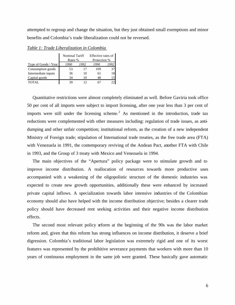
overnight. Table 1 gives some indications of the magnitude of the “Apertura”: in just a few

months, nominal average tariffs went from almost 40% to about 10% and the sectoral dispersion

of the protection rates also went down as shown by a dramatic reduction of the average effective

rate from almost 70% to just 22%. This move finally showed the government’s commitment to

free trade and imports surged. At a later stage in 1994, vested interests in protected sectors

1 This may be translated as “major shake-up”.

6

attempted to regroup and change the situation, but they just obtained small exemptions and minor

benefits and Colombia’s trade liberalization could not be reversed.

Table 1: Trade Liberalization in Colombia

Type of Goods \ Year 1990 1992 1990 1992Consumption goods 53 17 109 37Intermediate inputs 36 10 61 18Capital goods 34 10 48 15TOTAL 39 12 67 22

Nominal Tariff Rates %

Effective rates of Protection %

Quantitative restrictions were almost completely eliminated as well. Before Gaviria took office

50 per cent of all imports were subject to import licensing, after one year less than 3 per cent of

imports were still under the licensing scheme.2 As mentioned in the introduction, trade tax

reductions were complemented with other measures including: regulation of trade issues, as anti-

dumping and other unfair competition; institutional reform, as the creation of a new independent

Ministry of Foreign trade; stipulation of International trade treaties, as the free trade area (FTA)

with Venezuela in 1991, the contemporary reviving of the Andean Pact, another FTA with Chile

in 1993, and the Group of 3 treaty with Mexico and Venezuela in 1994.

The main objectives of the “Apertura” policy package were to stimulate growth and to

improve income distribution. A reallocation of resources towards more productive uses

accompanied with a weakening of the oligopolistic structure of the domestic industries was

expected to create new growth opportunities, additionally these were enhanced by increased

private capital inflows. A specialization towards labor intensive industries of the Colombian

economy should also have helped with the income distribution objective; besides a clearer trade

policy should have decreased rent seeking activities and their negative income distribution

effects.

The second most relevant policy reform at the beginning of the 90s was the labor market

reform and, given that this reform has strong influences on income distribution, it deserve a brief

digression. Colombia’s traditional labor legislation was extremely rigid and one of its worst

features was represented by the prohibitive severance payments that workers with more than 10

years of continuous employment in the same job were granted. These basically gave automatic

7

tenure to workers with more than 10 years on the job, but also reduced the possibility of a worker

to achieve that 10-year limit. In fact it has been calculated that only 2.5 workers out of 100 were

continuously employed for more than 10 years. This rigidity created serious employment stability

problems in the labor market and was eliminated with its reform. This also regulated more clearly

the hiring of temporary workers generating new employment opportunities especially for

unskilled workers. Kugler (1999) and Kugler and Cardenas (1999) provide empirical evidence

that this reform increased the Colombian labor market flexibility and its employment turnover.

As already mentioned, the late 80’s and the beginning of the 90’s witnessed a series of other

important structural reforms such as those affecting taxes, housing policy, exchange controls, port

regulations, central bank independence, financial (de)regulation, decentralization, social security

and privatization. Additionally, international prices for coffee and oil (the most important

exports) fluctuated around a lowering trend and other external shocks (mainly capital flows

volatility) affected the overall performance of Colombia.

Against this background of economic policy reforms and external shocks, the remaining part

of this section summarizes the evolution of poverty and inequality. At first sight, the described

economic reforms seem to have brought substantial welfare gains to Colombians. Between 1988

and 1995, mean per capita income had increased at a yearly rate of approximately 2.3 percent.

This increase only partially resulted in poverty reduction, since inequality, particularly between

rural and urban populations, worsened. Whereas urban mean per capita income rose by 3.2

percent per annum, rural incomes almost stagnated, growing at a rate lower than 1 percent per

annum.3

As shown in Table 2, a recent World Bank Poverty report (2002) finds that urban poverty has

declined significantly throughout the 1980s and the first half of the 1990s. According to this

assessment, rural poverty has remained relatively stable at high levels between 1988 and 1995

after important improvements in the 1980s. A UNDP study (1998) comes to different

conclusions. Overall poverty is found to be stable between 1988 and 1995. This stability is

mainly due to slightly improving poverty situation in urban areas, whereas rural poverty increases

significantly with a headcount ratio up from 63 to 69 percent.

2 It should be noted that, due to data deficiencies, the abolition of quantitative restrictions is not simulated in the

current version of the model. For more details on this sort of policy experiments see Bussolo and Roland-Holst (1999).

3 See World Bank (2002, p. 13). It should be noted that 1988 was an exceptionally prosperous year for agriculture due to the devaluation and a higher coffee production combined with higher coffee prices.

8

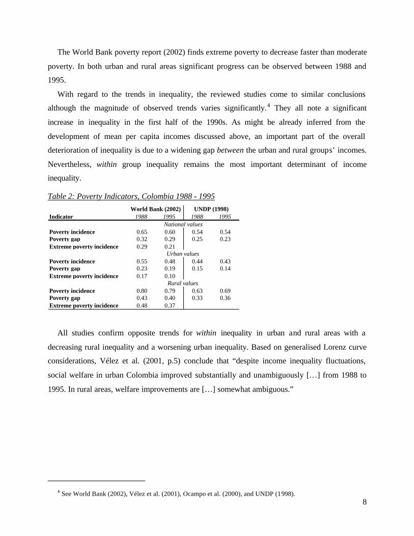
The World Bank poverty report (2002) finds extreme poverty to decrease faster than moderate

poverty. In both urban and rural areas significant progress can be observed between 1988 and

1995.

With regard to the trends in inequality, the reviewed studies come to similar conclusions

although the magnitude of observed trends varies significantly.4 They all note a significant

increase in inequality in the first half of the 1990s. As might be already inferred from the

development of mean per capita incomes discussed above, an important part of the overall

deterioration of inequality is due to a widening gap between the urban and rural groups’ incomes.

Nevertheless, within group inequality remains the most important determinant of income

inequality.

Table 2: Poverty Indicators, Colombia 1988 - 1995

Indicator 1988 1995 1988 1995

Poverty incidence 0.65 0.60 0.54 0.54Poverty gap 0.32 0.29 0.25 0.23Extreme poverty incidence 0.29 0.21



National values

Urban values

Rural values

World Bank (2002) UNDP (1998)

All studies confirm opposite trends for within inequality in urban and rural areas with a

decreasing rural inequality and a worsening urban inequality. Based on generalised Lorenz curve

considerations, Vélez et al. (2001, p.5) conclude that “despite income inequality fluctuations,

social welfare in urban Colombia improved substantially and unambiguously […] from 1988 to

1995. In rural areas, welfare improvements are […] somewhat ambiguous.”

4 See World Bank (2002), Vélez et al. (2001), Ocampo et al. (2000), and UNDP (1998).

9

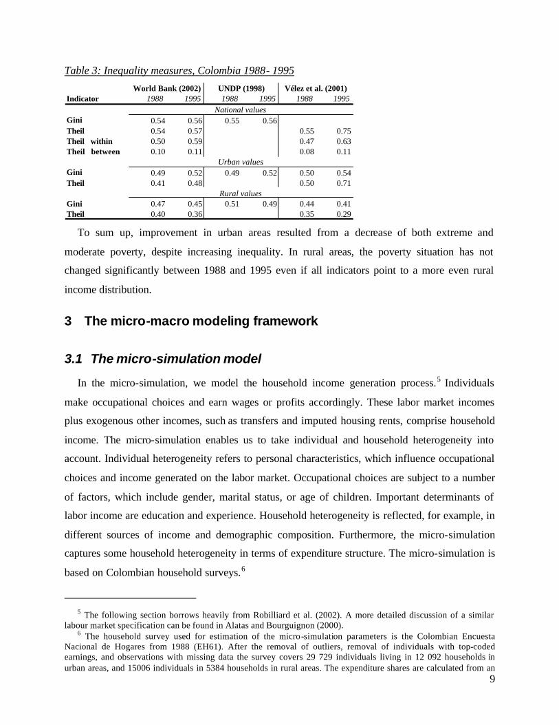
Table 3: Inequality measures, Colombia 1988- 1995

Indicator 1988 1995 1988 1995 1988 1995

Gini 0.54 0.56 0.55 0.56Theil 0.54 0.57 0.55 0.75Theil within 0.50 0.59 0.47 0.63Theil between 0.10 0.11 0.08 0.11

Gini 0.49 0.52 0.49 0.52 0.50 0.54Theil 0.41 0.48 0.50 0.71

Gini 0.47 0.45 0.51 0.49 0.44 0.41Theil 0.40 0.36 0.35 0.29

Urban values

Rural values

National values

Vélez et al. (2001)UNDP (1998)World Bank (2002)

To sum up, improvement in urban areas resulted from a decrease of both extreme and

moderate poverty, despite increasing inequality. In rural areas, the poverty situation has not

changed significantly between 1988 and 1995 even if all indicators point to a more even rural

income distribution.

3 The micro-macro modeling framework

3.1 The micro-simulation model

In the micro-simulation, we model the household income generation process.5 Individuals

make occupational choices and earn wages or profits accordingly. These labor market incomes

plus exogenous other incomes, such as transfers and imputed housing rents, comprise household

income. The micro-simulation enables us to take individual and household heterogeneity into

account. Individual heterogeneity refers to personal characteristics, which influence occupational

choices and income generated on the labor market. Occupational choices are subject to a number

of factors, which include gender, marital status, or age of children. Important determinants of

labor income are education and experience. Household heterogeneity is reflected, for example, in

different sources of income and demographic composition. Furthermore, the micro-simulation

captures some household heterogeneity in terms of expenditure structure. The micro-simulation is

based on Colombian household surveys.6

5 The following section borrows heavily from Robilliard et al. (2002). A more detailed discussion of a similar

labour market specification can be found in Alatas and Bourguignon (2000). 6 The household survey used for estimation of the micro-simulation parameters is the Colombian Encuesta

Nacional de Hogares from 1988 (EH61). After the removal of outliers, removal of individuals with top-coded earnings, and observations with missing data the survey covers 29 729 individuals living in 12 092 households in urban areas, and 15006 individuals in 5384 households in rural areas. The expenditure shares are calculated from an

10

Income Generation Model

The components of the income generation model are an occupational choice and an earnings

model. Individual agents can choose between inactivity, wage-employment, and self-

employment. In rural areas, there is a fourth option of being both wage-employed and self-

employed. The occupational choice model is assumed to be slightly different for household

heads, spouses, and other family members. As the possible occupational choices imply, earnings

are generated either in the form of wages for employees or as profits for the self-employed.

Individuals in rural areas can receive a mixed income from both types of activities. This latter

option will be ignored in the following illustration of the model. Being self-employed means

being part of wha t might be called a “household-enterprise”. All self-employed members of a

household pool their incomes. This pooled income is then called profit. The mechanisms of

profits earned in agriculture on the one hand side and other activities, such as petty trade, on the

other are assumed to be different. Since agriculture plays a negligible role in urban areas, this

differentiation is only implemented for rural areas.

The wage-employment market is segmented: the wage setting mechanisms are assumed to

differ between urban and rural areas, for skilled and unskilled labor, and for females and males,

which implies that there are eight wage labor market segments.

Household income comprises the labor income of all active household members and other

income. Wages and profits are thus the endogenous income sources of the household. All other

incomes are assumed to be exogenous and constant over time. The resulting total household

income is deflated with a household group specific price index, which takes into account the

differences in budget shares for food and non-food.

The income generation process, which consists of the occupational choice and the earnings

models, is first estimated using data from the Colombian household survey from 1988.7 The

estimated benchmark coefficients are then employed and changed in the micro-simulation.

Links to the CGE model

The micro-simulation and the CGE models are linked sequentially by a set of aggregate

variables. Specifically, firstly the CGE calculates the new equilibrium for a specific scenario, and

income and expenditure survey and matched with the EH61 based on household groups. For the problems of these datasets see Núñez and Jiménez (1997).

7 The occupational choice model was estimated using a multinomial logit. The wage equations were estimated by Ordinary Least Squares. Correcting for selection bias in these equations did not lead to major changes in the results

11

determines the following aggregate results: the average wage in each labor market segment, the

average profits for different activities, the shares of self- and wage-employed for each segment

(labor force composition), and the relative price of food and non-food commodities. Then, these

aggregate variables are used as targets for the micro-simulation model where individual changes

in earnings and labor force composition are computed. These micro changes are obtained by

varying coefficients in the occupational choice and the earnings models. Coefficients are

adjusted, and occupational choices and earnings change accordingly, until the results of the

micro-simulation are consistent, at an aggregate level, with the results from the CGE model.

Elements of the Model

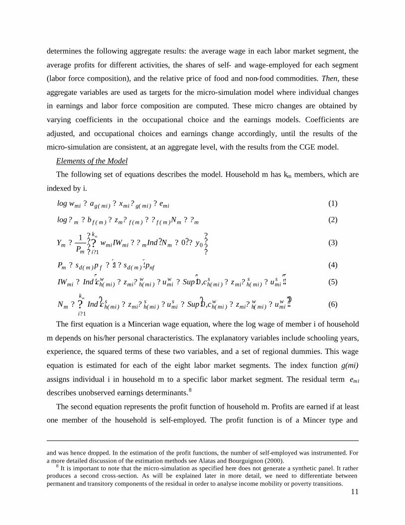
The following set of equations describes the model. Household m has km members, which are

indexed by i.

mi)mi(gmi)mi(gmi exawlog ??? ? (1)

mm)m(f)m(fm)m(fm Nzblog ???? ???? (2)

? ? ???

????

????? ?

?0

10

1yNIndIWw

PY mm

k

imimi

mm

m

? (3)

? ? nf)m(df)m(dm pspsP ??? 1 (4)

? ?? ?smi

s)mi(hmi

s)mi(h

wmi

w)mi(hmi

w)mi(hmi uzc,SupuzcIndIW ?????? ?? 0 (5)

? ?? ???

??????mk

i

wmi

w)mi(hmi

w)mi(h

smi

s)mi(hmi

s)mi(hm uzc,SupuzcIndN

10 ?? (6)

The first equation is a Mincerian wage equation, where the log wage of member i of household

m depends on his/her personal characteristics. The explanatory variables include schooling years,

experience, the squared terms of these two variables, and a set of regional dummies. This wage

equation is estimated for each of the eight labor market segments. The index function g(mi)

assigns individual i in household m to a specific labor market segment. The residual term emi

describes unobserved earnings determinants.8

The second equation represents the profit function of household m. Profits are earned if at least

one member of the household is self-employed. The profit function is of a Mincer type and

and was hence dropped. In the estimation of the profit functions, the number of self-employed was instrumented. For a more detailed discussion of the estimation methods see Alatas and Bourguignon (2000).

8 It is important to note that the micro-simulation as specified here does not generate a synthetic panel. It rather produces a second cross-section. As will be explained later in more detail, we need to differentiate between permanent and transitory components of the residual in order to analyse income mobility or poverty transitions.

12

includes as explanatory variables the schooling of the household head, her/his experience plus the

squared terms the former two variables, and regional dummies. Of course, profits also depend on

the number of self-employed in household m, Nm. The residual ?m captures unobserved effects.

The index function f(m) denotes whether a household earns profits in urban or rural areas.

Furthermore, different profit functions for agricultural, non-agricultural, and mixed activities are

estimated in rural areas.

Family income is defined by the third equation. It consists of the wages and profits earned by

the family members and an exogenous income y0m . This exogenous income corresponds to “other

income” in the survey and may include government transfers, transfers from abroad, capital

income, etc.. IWmi is a dummy variable that equals 1 if member i of the household is wage-

employed and 0 otherwise. Likewise, profits will only be earned if at least one family member is

self-employed (Nm>0). Family income is deflated by a household specific price index.

This household specific price index is defined by equation (4). The parameter s denotes the

expenditure shares for food- and non-food. These shares are calculated by household income

quintiles. Note that the prices pf for food and pnf for non-food are generated in the CGE model.

The index function d(m) indicates to which of the five income brackets household m belongs and

which food expenditure share is assigned to the household.

The fifth equation explains the aforementioned dummy IWmi. The individual will be wage-

employed if the utility associated with wage-employment is higher than the utility of being self-

employed or inactive. The utility of being inactive is arbitrarily set to zero, whereas the utilities of

the employment options depend on a set of personal and family characteristics, zmi. These

characteristics include gender, marital status, education, experience, other income, the

educational attainments of other family members, and the number of children. Unobserved

determinants of occupational choices are represented by the residuals.

Equation (6) gives the number of self-employed. Similar to the choice in equation (5), the

individual i of household m will prefer self-employment if the associated utility is higher than the

utility of inactivity or wage-employment. The self-employed household members form the

“household enterprise” with Nm working members. Thus, the last two equations represent the

occupational choices of the household members. The occupational choice model is estimated

separately for household heads, spouses, and other family members in urban and rural areas. The

index function h(mi) assigns the individual to the corresponding group.

13

The model just described gives the household income as a non- linear function of individual

and household characteristics, unobserved characteristics, and the household budget shares. This

function depends on three sets of parameters, which are estimated based on the 1988 survey.

These parameters include (1) the parameters of the wage equation for each labor market segment,

(2) the parameters of the profit function for “household enterprises” in urban areas and different

activities in rural areas, (3) the parameters in the utility associated with different occupational

choices for heads, spouses, and other family members. As will be explained later in more detail,

some of these parameters are changed in order to produce the aggregate results with regard to

wages, profits, and employment shares given by the CGE. The CGE also gives the price vector,

which in a last step is used to deflate family income.

Remarks on the Labor Market Specification

The income generation model requires some comments on the assumptions behind its

formulation. First of all, despite the availability of data on working time we decided to model the

occupational choice as a discrete choice.9 Secondly, our model assumes that the Colombian labor

market is segmented along different lines. One line of segmentation separates wage-employment

from self-employment. In a perfectly competitive labor market, the returns to labor would be

equal for these two types of employment. Yet, segmentation may be justified because income

from self-employment is likely to contain a rent from non- labor assets used, and its clearing

mechanism may differ from that of wage employment. Information on non- labor assets, land in

rural areas and at least a small amount of capital in urban areas, is not available for Colombia,

hence distinct equations need to be estimated even if the labor markets were competitive. In

addition, even in those cases where information on non-labor assets is available, a segmented

labor market can be justified by the fact that wage-employment may be rationed and self-

employment thus “absorbs” those who do not get a job in the preferred wage work. Wage work

could be preferred for generating a more steady income stream or for fringe benefits related to

this type of employment. Conversely, self-employment might exhibit important externalities, for

example for families in which children have to be taken care of. Self-employment of the

household head may also create employment opportunities for other family members.

Additional segmentation is assumed within the wage labor market. The segmentation

hypothesis along the lines of different gender, skill, and area is strongly supported by the

9 However, estimating wage equations based on hourly wages did not make a major difference in the coefficients.

14

regression results. The same holds for the estimation of different profit functions for agricultural

and non-agricultural activities in rural areas.

Estimation of the occupational choice and earnings equations

As mentioned above, the occupational choice model and the wage and profits equations are

estimated in a first step in order to obtain an initial set of coefficients (aG, ? G, bF, ? F, cHw, ? H

w,

cHs, ? H

s) and unobserved characteristics (emi, ?mi, uwmi, us

mi). Unobserved characteris tics say for

the wage equation can of course only be obtained for those who are actually wage-employed. For

self-employed or inactive individuals the unobserved characteristics in the wage-equation are

generated by drawing random numbers from a normal distribution. In the same way, we generate

unobserved characteristics for the profit function for households in which nobody is self-

employed. As we estimate wage and profit functions using ordinary least squares, we assume

these unobserved characteristics to be normally distributed. Additionally, unobserved

characteristics need to be generated for the occupational choice model. These residuals are

assumed to be distributed according to the double exponential law since we estimate a

multinomial logit model. They were drawn randomly consistent with the observed occupational

choice, i.e. the utility a wage earner relates to wage-employment has to be higher than the utility

associated with inactivity or self-employment.

Macro-Micro Links in Detail

As already mentioned, the micro-simulation and the CGE models are linked in a sequential

fashion. In a first stage a shock is simulated in the CGE model and then the micro-simulation

adjusts micro data so that values for its aggregate variables are consistent with the CGE macro

equilibrium. Consistency requires that across the two models the following items are equal: (1)

the changes in average wages in each segment, (2) the changes in average profits in each activity,

(3) the changes in employment shares in each segment, i.e. the shares of wage-earners, self-

employed, and inactive individuals per segment, and (4) the food and non food commodities price

changes. The CGE is initially calibrated in such a way that it is consistent with the benchmark

micro-simulation. This benchmark micro-simulation is produced by using the set of initial

coefficients and unobserved characteristics obtained through the estimation work just described.10

Formally, the following constraints describe the consistency requirements.

10 By doing this, we simply reproduce the original dataset.

15

? ?? ? GG)mi(g,i

smi

s)mi(hmi

s)mi(h

wmi

w)mi(hmi

w)mi(h

m

G)mi(g,imi

^

m

Euˆzc,SupuˆzcInd

IW

??????

?

??

??

?

?

?? 0 (7)

? ?? ? GG)mi(g,i

wmi

w)mi(hmi

w)mi(h

smi

s)mi(hmi

s)mi(h

mSuˆzc,SupuˆzcInd ????????

??? 0 (8)

? ????

???G)mi(g,i

Gmi^

miGmiGm

wIWeˆxaexp ? (9)

? ? ? ? FF)m(f,m

mmGmG NIndˆˆzbexp ?? ???????

0 (10)

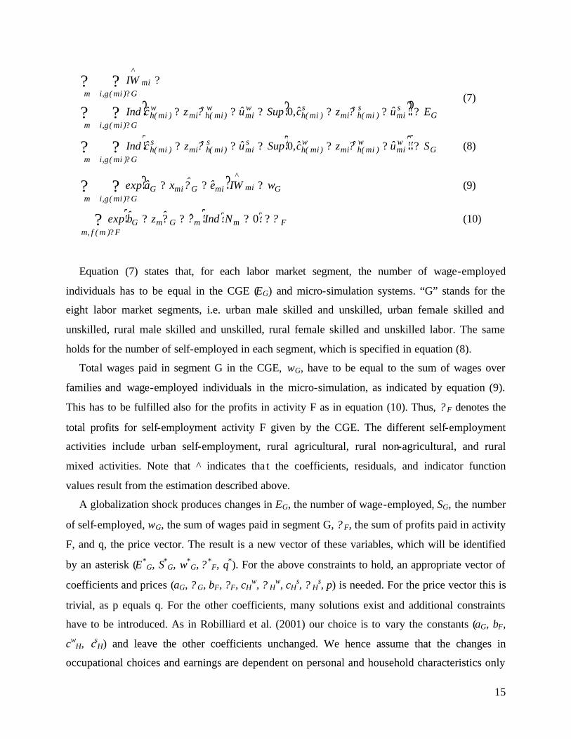
Equation (7) states that, for each labor market segment, the number of wage-employed

individuals has to be equal in the CGE (EG) and micro-simulation systems. “G” stands for the

eight labor market segments, i.e. urban male skilled and unskilled, urban female skilled and

unskilled, rural male skilled and unskilled, rural female skilled and unskilled labor. The same

holds for the number of self-employed in each segment, which is specified in equation (8).

Total wages paid in segment G in the CGE, wG, have to be equal to the sum of wages over

families and wage-employed individuals in the micro-simulation, as indicated by equation (9).

This has to be fulfilled also for the profits in activity F as in equation (10). Thus, ? F denotes the

total profits for self-employment activity F given by the CGE. The different self-employment

activities include urban self-employment, rural agricultural, rural non-agricultural, and rural

mixed activities. Note that ^ indicates tha t the coefficients, residuals, and indicator function

values result from the estimation described above.

A globalization shock produces changes in EG, the number of wage-employed, SG, the number

of self-employed, wG, the sum of wages paid in segment G, ? F, the sum of profits paid in activity

F, and q, the price vector. The result is a new vector of these variables, which will be identified

by an asterisk (E*G, S*

G, w*G, ? *

F, q*). For the above constraints to hold, an appropriate vector of

coefficients and prices (aG, ? G, bF, ?F, cHw, ? H

w, cHs, ? H

s, p) is needed. For the price vector this is

trivial, as p equals q. For the other coefficients, many solutions exist and additional constraints

have to be introduced. As in Robilliard et al. (2001) our choice is to vary the constants (aG, bF,

cwH, cs

H) and leave the other coefficients unchanged. We hence assume that the changes in

occupational choices and earnings are dependent on personal and household characteristics only

16

to a limited degree. Changing the intercept in one of the wage equations implies that all

individuals of the respective segment experience the same increase in log earnings. This increase

does not depend on individual characteristics. The same holds for the profit functions. With

regard to the occupational choice, it should be noted that the CGE does not allow for

distinguishing between the choices of heads, spouses, and others. The changes are thus the same

across these groups.

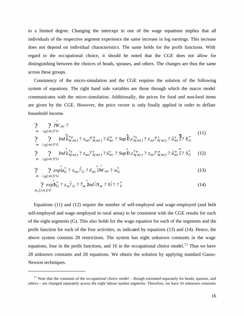
Consistency of the micro-simulation and the CGE requires the solution of the following

system of equations. The right hand side variables are those through which the macro model

communicates with the micro-simulation. Additionally, the prices for food and non-food items

are given by the CGE. However, the price vector is only finally applied in order to deflate

household income.

? ?? ? *G

smi

s)mi(hmi

s*)mi(h

wmi

w)mi(hmi

w*)mi(h

G)mi(g,im

G)mi(g,imi

^

m

Euˆzc,SupuˆzcInd

IW

??????

?

??

??

?

?

?? 0 (11)

? ?? ? *G

wmi

w)mi(hmi

w*)mi(h

smi

s)mi(hmi

s*)mi(h

G)mi(g,imSuˆzc,SupuˆzcInd ????????

??? 0 (12)

? ????

???G)mi(g,i

*Gmi

^

miGmi*G

mwIWeˆxaexp ? (13)

? ? ? ? *F

F)m(f,mmmGm

*G NIndˆˆzbexp ?? ??????

?0 (14)

Equations (11) and (12) require the number of self-employed and wage-employed (and both

self-employed and wage-employed in rural areas) to be consistent with the CGE results for each

of the eight segments (G). This also holds for the wage equation for each of the segments and the

profit function for each of the four activities, as indicated by equations (13) and (14). Hence, the

above system contains 28 restrictions. The system has eight unknown constants in the wage

equations, four in the profit functions, and 16 in the occupational choice model.11 Thus we have

28 unknown constants and 28 equations. We obtain the solution by applying standard Gauss-

Newton techniques.

11 Note that the constants of the occupational choice model – though estimated separately for heads, spouses, and

others – are changed separately across the eight labour market segments. Therefore, we have 16 unknown constants

17

Solving the above system gives us a new set of constants (a*G, b*

F, c*wH, c*s

H), which is then

used to compute occupational choices, wages, and profits. The resulting household incomes are

deflated by the household group specific price index derived from the CGE results for food and

non-food prices.

Linking the CGE and the micro-simulation in the way described above goes beyond simply

rescaling various household income sources or reweighing households dependent on the

occupation of its members, which is what the RHG approach does. The simulation model takes

the different sources of household income into account and mimics individual occupational

choices, based on a wide range of individual characteristics, and it is therefore a more accurate

method than just rescaling household groups incomes.

An Artificial Panel data set?

At first sight, one may be inclined to think that the simulation method generates a kind of

artificial panel, which would be most helpful and interesting from an analytical point of view. If

we want to analyze poverty dynamics, we need to trace individuals and households across time.

However, to produce a synthetic panel further assumptions need to be introduced. For brevity, the

arising problems are illustrated for the case of the wage equation, but they apply to all the

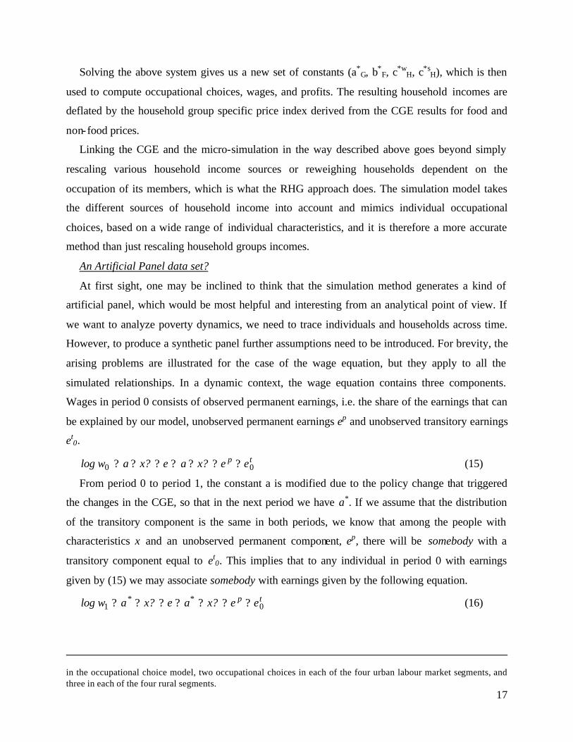
simulated relationships. In a dynamic context, the wage equation contains three components.

Wages in period 0 consists of observed permanent earnings, i.e. the share of the earnings that can

be explained by our model, unobserved permanent earnings ep and unobserved transitory earnings

et0.

tp eexaexawlog 00 ??????? ?? (15)

From period 0 to period 1, the constant a is modified due to the policy change that triggered

the changes in the CGE, so that in the next period we have a*. If we assume that the distribution

of the transitory component is the same in both periods, we know that among the people with

characteristics x and an unobserved permanent component, ep, there will be somebody with a

transitory component equal to et0. This implies that to any individual in period 0 with earnings

given by (15) we may associate somebody with earnings given by the following equation.

tp** eexaexawlog 01 ??????? ?? (16)

in the occupational choice model, two occupational choices in each of the four urban labour market segments, and three in each of the four rural segments.

18

The individual with earnings given by (16) is not the same as the individual whose earnings

were represented by (15). Since this is what we do in the micro-simulation, as set up to this point,

we do not generate a synthetic panel, but two cross-sections. Based on two-cross-sections it is of

course not possible to trace individuals through time. Yet, there is no problem if we compute

aggregate inequality and poverty indicators, which we compare across time. In order to study

poverty dynamics though we would have to make sure that we could identify the individuals of

the households who cross the poverty line. It is therefore not sufficient to associate somebody

with unobserved earnings, but a specific individual.

The reason why we cannot simulate a panel arises from the fact that we cannot differentiate

between the two unobserved components. However, introducing a set of assumptions with regard

to these two terms helps. First, we assume the transitory component to be independent and

identically distributed across time. Second, we have to make an assumption about the proportions

of the variance of the entire residual term e that is due to the respective components. There are

though a number of difficulties related to this method, in particular to the specification of the

variance proportions. Some empirical estimates of these proportions can be found in Atkinson et

al. (1992) where a number of empirical studies on earnings mobility are surveyed. They find the

proportions of the three components in an earnings panel model to differ substantially across

different studies. Of course, the total unobserved component is smaller the better the model

explains log earnings. The proportion of the transitory component in log earnings covariance

varies between less than 10 and 30 percent over long time horizons of more than 10 years. We are

not aware of empirical work on earnings mobility in developing countries, which would analyze

these issues in detail. There is scope for further research on earnings mobility as some panel

datasets have become available. Assuming a small proportion of transitory earnings in developing

economies in general may be justified by a number of arguments. Social mobility is generally

lower in developing countries.12 From this, we may infer that transitory earnings account for a

smaller proportion of earnings. Additionally, recent research has shown that income shocks

remain after a considerable period of time, which also would imply less importance of a

transitory component, at least in the short run. 13 On the other hand, the transitory component may

12 For social mobility in Latin America see Andersen (2000). 13 See Newhouse (2001) who studies the persistence of transient income shocks to farm households in rural

Indonesia. He finds, for example that “about 40 percent of household income shocks remain after four years.”

19

be particularly important for small farms, which are exposed to a number of transitory, primarily

environmental, risks.

For the purpose of the poverty transition analysis, we simulated a panel based on the

aforementioned assumptions. These panel-based results are of a preliminary character and should

be treated with caution, as further research in this field is needed. Experimenting with different

proportions in the micro-simulation had a substantial impact on the results. Reducing the

proportion of the variance of the residual term e, which is due to the transitory component, to 10

percent produced results in the historical simulation, which were close to those of the original

simulation of two cross-sections. Using higher proportions due to the transitory component

resulted in considerable increases in inequality indicators. The poverty transition analysis is thus

based on the assumption that only 10 percent of the unobserved effects are transitory. 14

3.2 The CGE model

The 1988 Social Accounting Matrix (SAM) has been used as the initial benchmark

equilibrium for the CGE model. The SAM, which includes 36 sectors, 20 commodities, 9 factors

(8 labor categories and 1 composite capital), 2 households (urban and rural), and other accounts

(government, savings and investment, and rest of the world), has been assembled from various

sources incorporating data from the 1988 Input Output table, the 1988 households surveys and

from a 1994 SAM.15

The CGE model is based on a standard neoclassical general equilibrium model; however, to

take into account special features of the Colombian economy, it differs from the typical

specification in two important aspects: production sectors are distinguished between formal and

informal activities, and the associated labor markets present structural imperfections with

different clearing mechanisms for the formal and informal sectors.16

14 As mentioned before, aggregate inequality indicators increased under the synthetic panel approach. This

increase was more pronounced the higher the share of the transitory component. We understood these results when we had a look at the distribution of unobserved earnings. For lower incomes, the distribution of unobserved earnings is skewed to the right, hence implying relatively high unobserved earnings. For higher incomes, the distribution of the entire residual resembles a normal distribution. If we substitute these unobserved earnings or a portion of it by generated normally distributed unobserved earnings, we thus “redistribute” income from the poor to the rich, thereby increasing inequality.

15 For more details on the SAM see Bussolo and Correa (1999). 16 The CGE model used here is the result of merging the CGE model built for Colombia and described in Bussolo

et al (1998), and that constructed for the Indonesia case study mentioned in Robilliard et al (2001) and more fully discussed in Löfgren et al (2001).

20

Production

Output results from nested CES (Constant Elasticity of Substitution) functions that, at the top

level, combine intermediate and value added aggregates. At the second level, on the one hand, the

intermediate aggregate is obtained combining all products in fixed proportions (Leontief

structure), and, on the other hand, value added results by aggregating the 9 primary factors.

Formal and informal activities differ primarily by employing different labor types, with the

former using exclusively wage-workers and the latter using exclusively self-employment.

Additionally, informal activities are, on average, less capital intensive. These features, together

with the disaggregation of 8 labor categories, allow to model in a more realistic way the

segmented Colombian labor markets and to capture the dualistic nature of the economy of this

country. On the demand side, each commodity is represented by a composite which includes

outputs from formal and informal activities. Imperfect substitutability between formal and

informal components of the same commodity is assumed and flexible domestic prices adjust to

reach equilibrium between domestic demand and supply.

Income Distribution and Absorption

Labor income and capital revenues are allocated to households according to a fixed coefficient

distribution matrix derived from the original SAM. Private consumption demand is obtained

through maximization of household specific utility function following the Linear Expenditure

System (LES). Household utility is a function of consumption of different goods. Income

elasticities are different for each household and product and vary in the range 0.20, for basic

products consumed by the household with highest income, to 1.30 for services. Once their total

value is determined, government and investment demands17 are disaggregated in sectoral

demands according to fixed coefficient functions.

International Trade

In the model we assume imperfect substitution among goods originating in different

geographical areas.18 Imports demand results from a CES aggregation function of domestic and

imported goods. Export supply is symmetrically modeled as a Constant Elasticity of

Transformation (CET) function. Producers decide to allocate their output to domestic or foreign

markets responding to relative prices. As Colombia is unable to influence world prices, the small

17 Aggregate investment is set equal to aggregate savings, while aggregate government expenditures are

exogenously fixed. 18 See Armington (1969) for details.

21

country assumption holds, and its imports and exports prices are treated as exogenous. The

assumptions of imperfect substitution and imperfect transformability grant a certain degree of

autonomy of domestic prices with respect to foreign prices and prevent the model to generate

corner solutions; additionally they also permit to model cross-hauling a feature normally

observed in real economies. The balance of payments equilibrium is determined by the equality

of foreign savings (which are exogenous) to the value for the current account. With fixed world

prices and capital inflows, all adjustments are accommodated by changes in the real exchange

rate: increased import demand, due to trade liberalization must be financed by increased exports,

and these can expand owing to the improved resource allocation. Price decreases in importables

drive resources towards export sectors and contribute to falling domestic resource costs (or real

exchange rate depreciation).

Factor Markets

Labor is distinguished into 8 categories: Urban Male Skilled, Urban Male Unskilled, Urban

Female Skilled, Urban Female Unskilled, Rural Male Skilled, Rural Male Unskilled, Rural

Female Skilled, and Rural Female Unskilled. These categories are considered imperfectly

substitutable inputs in the production process; additionally, to take into account the fact that the

labor market for self-employment and that for wage-employment adjust differently, the model

assumes that labor markets are segmented between formal and informal sectors. In particular,

given that wage-employment enjoys formal protection, such as unions wage setting and minimum

wages, a certain degree of formal wage inflexibility is implemented in the model through a wage

curve. The equilibrium in the formal market is thus determined by the intersection of the firms’

labor demand and this wage curve. The informal labor market adjusts residually so that, for each

of the eight mentioned categories, total supply (formal plus informal labor) is kept fixed. Capital

is an aggregate factor and includes fixed capital as well as land; formal sectors show higher

capital intensities than informal ones.

To take into account the medium term horizon of the model, i.e. the time period considered

necessary to a trade shock to work through the economy, both labor and capital are perfectly

mobile across sectors but their aggregate supplies are fixed.

Model Closures

The equilibrium condition on the balance of payments is combined with other closure

conditions so that the model can be solved for each period. Firstly consider the government

budget. Its surplus is fixed and the household income tax schedule shifts in order to achieve the

22

predetermined net government position. Secondly, investment must equal savings, which

originate from households, corporations, government and rest of the world. Aggregate investment

is set equal to aggregate savings, while aggregate government expenditures are exogenously

fixed.

4 Simulations and Results

Two main scenarios have been analyzed with the methodology described in the previous

section: in the first ‘historical’ scenario, the micro-simulation system, which was estimated on the

1988 survey, is shocked in such a way that its final aggregate variables for employment

composition and wages correspond to the values recorded in the 1995 survey; in this scenario, the

CGE model is not used. In the second ‘trade liberalization’ scenario, the CGE model is used to

simulate tariff abatement and to obtain general equilibrium values for employment and wages

which are then used to shock the micro-simulation model. In this way, two new income

distributions are derived: the first includes all the shocks (as reflected in the observed historical

changes in aggregate employment and wages) occurred between 1988 and 1995, and the second

includes only the shocks directly attributable to trade policy. Before comparing these two new

distributions and thus assessing the weight trade shocks have in explaining overall poverty and

inequality evolutions, a closer look at the socio-economic characteristics and income sources of

the poor, and at the ‘historical’ and ‘trade’ shocks on aggregate variables is quite useful.

4.1 The Colombian Poor, and the Historical and Trade Shocks

The 1988 Colombia poverty profile corresponds quite closely to that of a typical developing

country: the majority of the poor live in rural areas, are unemployed, or, when working, they are

in the unskilled informal segment of the labor market. To facilitate the interpretation of the micro

results of the next sub-section, the poverty data from the 1988 survey have been reorganized to

correspond directly to the labor market specification chosen for our model: Table 4 shows a

poverty profile according to the occupational choice of the household head, and Table 5 considers

the rural/urban distribution and the labor market segments.

23

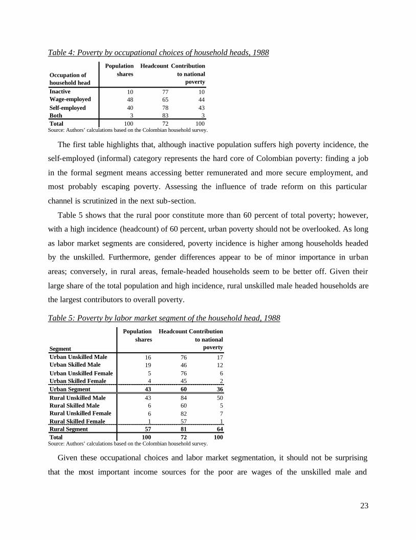
Table 4: Poverty by occupational choices of household heads, 1988

Occupation of household head

Population shares

Headcount Contribution to national

poverty

Inactive 10 77 10Wage-employed 48 65 44Self-employed 40 78 43Both 3 83 3Total 100 72 100

Source: Authors’ calculations based on the Colombian household survey.

The first table highlights that, although inactive population suffers high poverty incidence, the

self-employed (informal) category represents the hard core of Colombian poverty: finding a job

in the formal segment means accessing better remunerated and more secure employment, and

most probably escaping poverty. Assessing the influence of trade reform on this particular

channel is scrutinized in the next sub-section.

Table 5 shows that the rural poor constitute more than 60 percent of total poverty; however,

with a high incidence (headcount) of 60 percent, urban poverty should not be overlooked. As long

as labor market segments are considered, poverty incidence is higher among households headed

by the unskilled. Furthermore, gender differences appear to be of minor importance in urban

areas; conversely, in rural areas, female-headed households seem to be better off. Given their

large share of the total population and high incidence, rural unskilled male headed households are

the largest contributors to overall poverty.

Table 5: Poverty by labor market segment of the household head, 1988

Segment

Population shares

Headcount Contribution to national

poverty

Urban Unskilled Male 16 76 17Urban Skilled Male 19 46 12Urban Unskilled Female 5 76 6Urban Skilled Female 4 45 2Urban Segment 43 60 36Rural Unskilled Male 43 84 50Rural Skilled Male 6 60 5Rural Unskilled Female 6 82 7Rural Skilled Female 1 57 1Rural Segment 57 81 64Total 100 72 100

Source: Authors’ calculations based on the Colombian household survey.

Given these occupational choices and labor market segmentation, it should not be surprising

that the most important income sources for the poor are wages of the unskilled male and

24

agricultural profits; once again, significant poverty reduction can be achieved when these types of

income are positively affected.

The effects of historical and trade scenarios on the aggregate employment and income

categories are analyzed in the remaining part of this section.

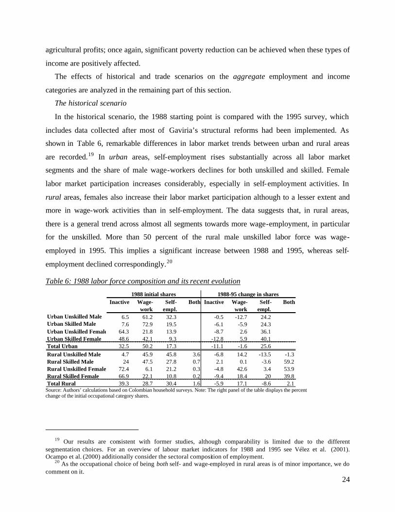
The historical scenario

In the historical scenario, the 1988 starting point is compared with the 1995 survey, which

includes data collected after most of Gaviria’s structural reforms had been implemented. As

shown in Table 6, remarkable differences in labor market trends between urban and rural areas

are recorded.19 In urban areas, self-employment rises substantially across all labor market

segments and the share of male wage-workers declines for both unskilled and skilled. Female

labor market participation increases considerably, especially in self-employment activities. In

rural areas, females also increase their labor market participation although to a lesser extent and

more in wage-work activities than in self-employment. The data suggests that, in rural areas,

there is a general trend across almost all segments towards more wage-employment, in particular

for the unskilled. More than 50 percent of the rural male unskilled labor force was wage-

employed in 1995. This implies a significant increase between 1988 and 1995, whereas self-

employment declined correspondingly.20

Table 6: 1988 labor force composition and its recent evolution

Inactive Wage-work

Self-empl.

Both Inactive Wage-work

Self-empl.

Both

Urban Unskilled Male 6.5 61.2 32.3 -0.5 -12.7 24.2Urban Skilled Male 7.6 72.9 19.5 -6.1 -5.9 24.3Urban Unskilled Female 64.3 21.8 13.9 -8.7 2.6 36.1Urban Skilled Female 48.6 42.1 9.3 -12.8 5.9 40.1Total Urban 32.5 50.2 17.3 -11.1 -1.6 25.6Rural Unskilled Male 4.7 45.9 45.8 3.6 -6.8 14.2 -13.5 -1.3Rural Skilled Male 24 47.5 27.8 0.7 2.1 0.1 -3.6 59.2Rural Unskilled Female 72.4 6.1 21.2 0.3 -4.8 42.6 3.4 53.9Rural Skilled Female 66.9 22.1 10.8 0.2 -9.4 18.4 20 39.8Total Rural 39.3 28.7 30.4 1.6 -5.9 17.1 -8.6 2.1

1988 initial shares 1988-95 change in shares

Source: Authors’ calculations based on Colombian household surveys. Note: The right panel of the table displays the percent change of the initial occupational category shares.

19 Our results are consistent with former studies, although comparability is limited due to the different

segmentation choices. For an overview of labour market indicators for 1988 and 1995 see Vélez et al. (2001). Ocampo et al. (2000) additionally consider the sectoral composition of employment.

20 As the occupational choice of being both self- and wage-employed in rural areas is of minor importance, we do comment on it.

25

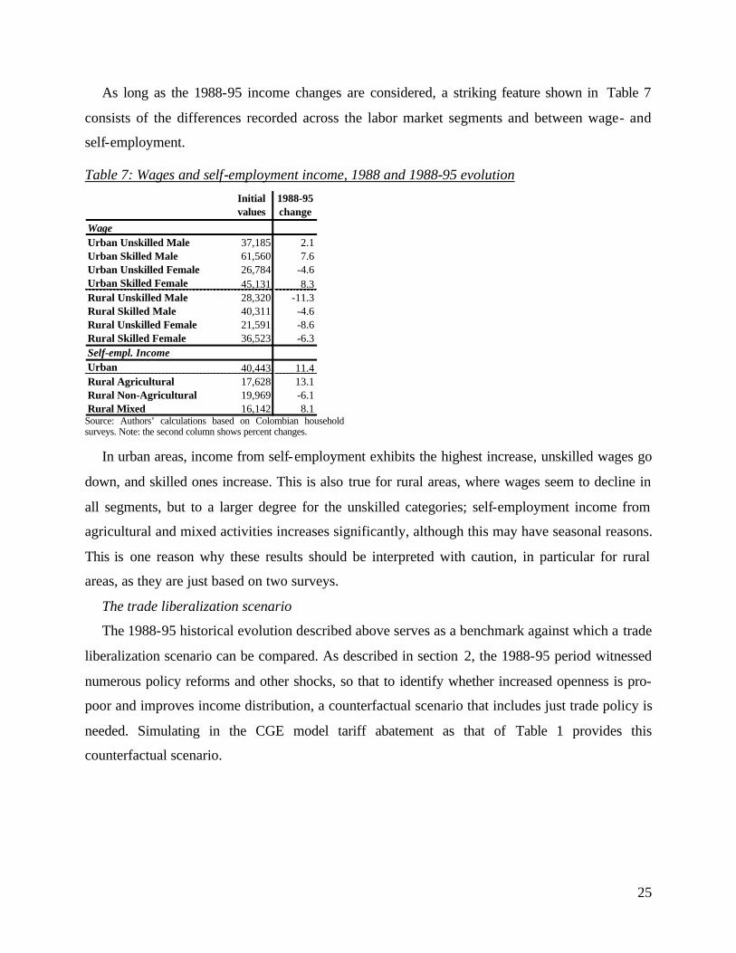
As long as the 1988-95 income changes are considered, a striking feature shown in Table 7

consists of the differences recorded across the labor market segments and between wage- and

self-employment.

Table 7: Wages and self-employment income, 1988 and 1988-95 evolution

Initial values

1988-95 change

WageUrban Unskilled Male 37,185 2.1Urban Skilled Male 61,560 7.6Urban Unskilled Female 26,784 -4.6Urban Skilled Female 45,131 8.3Rural Unskilled Male 28,320 -11.3Rural Skilled Male 40,311 -4.6Rural Unskilled Female 21,591 -8.6Rural Skilled Female 36,523 -6.3Self-empl. IncomeUrban 40,443 11.4Rural Agricultural 17,628 13.1Rural Non-Agricultural 19,969 -6.1Rural Mixed 16,142 8.1

Source: Authors’ calculations based on Colombian household surveys. Note: the second column shows percent changes.

In urban areas, income from self-employment exhibits the highest increase, unskilled wages go

down, and skilled ones increase. This is also true for rural areas, where wages seem to decline in

all segments, but to a larger degree for the unskilled categories; self-employment income from

agricultural and mixed activities increases significantly, although this may have seasonal reasons.

This is one reason why these results should be interpreted with caution, in particular for rural

areas, as they are just based on two surveys.

The trade liberalization scenario

The 1988-95 historical evolution described above serves as a benchmark against which a trade

liberalization scenario can be compared. As described in section 2, the 1988-95 period witnessed

numerous policy reforms and other shocks, so that to identify whether increased openness is pro-

poor and improves income distribution, a counterfactual scenario that includes just trade policy is

needed. Simulating in the CGE model tariff abatement as that of Table 1 provides this

counterfactual scenario.

26

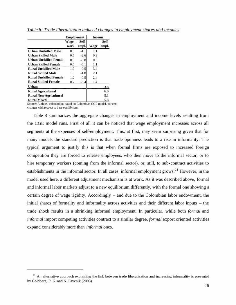
Table 8: Trade liberalization induced changes in employment shares and incomes

Wage-work

Self-empl. Wage

Self-empl.

Urban Unskilled Male 0.5 -1.1 1.1Urban Skilled Male 0.5 -2.6 0.9Urban Unskilled Female 0.3 -0.8 0.5Urban Skilled Female 0.5 -6.1 1.1Rural Unskilled Male 1.7 -0.5 3.4Rural Skilled Male 1.0 -1.8 2.1Rural Unskilled Female 1.2 -0.5 2.4Rural Skilled Female 0.7 -5.4 1.4Urban 3.8Rural Agricultural 6.6Rural Non-Agricultural 5.1Rural Mixed 5.8

Employment Income

Source: Authors’ calculations based on Colombian CGE model, per cent changes with respect to base equilibrium.

Table 8 summarizes the aggregate changes in employment and income levels resulting from

the CGE model runs. First of all it can be noticed that wage employment increases across all

segments at the expenses of self-employment. This, at first, may seem surprising given that for

many models the standard prediction is that trade openness leads to a rise in informality. The

typical argument to justify this is that when formal firms are exposed to increased foreign

competition they are forced to release employees, who then move to the informal sector, or to

hire temporary workers (coming from the informal sector), or, still, to sub-contract activities to

establishments in the informal sector. In all cases, informal employment grows.21 However, in the

model used here, a different adjustment mechanism is at work. As it was described above, formal

and informal labor markets adjust to a new equilibrium differently, with the formal one showing a

certain degree of wage rigidity. Accordingly – and due to the Colombian labor endowment, the

initial shares of formality and informality across activities and their different labor inputs – the

trade shock results in a shrinking informal employment. In particular, while both formal and

informal import competing activities contract to a similar degree, formal export oriented activities

expand considerably more than informal ones.

21 An alternative approach explaining the link between trade liberalization and increasing informality is presented

by Goldberg, P. K. and N. Pavcnik (2003).

27

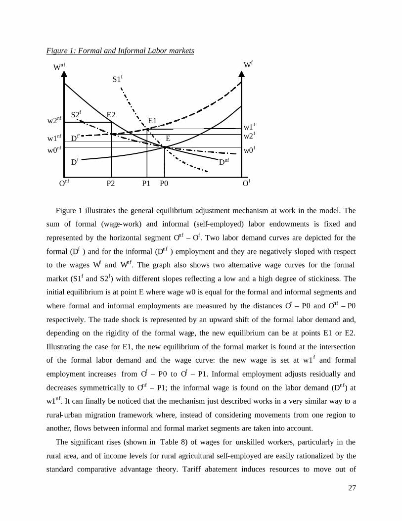
Figure 1: Formal and Informal Labor markets

E

E1 E2

Wnf S1f

S2f

Df

Df’

Dnf

Wf

Onf Of

w2f w1 f

w0f

P0 P1 P2

w2nf

w0nf

w1nf

Figure 1 illustrates the general equilibrium adjustment mechanism at work in the model. The

sum of formal (wage-work) and informal (self-employed) labor endowments is fixed and

represented by the horizontal segment Onf – Of. Two labor demand curves are depicted for the

formal (Df ) and for the informal (Dnf ) employment and they are negatively sloped with respect

to the wages Wf and Wnf. The graph also shows two alternative wage curves for the formal

market (S1f and S2f) with different slopes reflecting a low and a high degree of stickiness. The

initial equilibrium is at point E where wage w0 is equal for the formal and informal segments and

where formal and informal employments are measured by the distances Of – P0 and Onf – P0

respectively. The trade shock is represented by an upward shift of the formal labor demand and,

depending on the rigidity of the formal wage, the new equilibrium can be at points E1 or E2.

Illustrating the case for E1, the new equilibrium of the formal market is found at the intersection

of the formal labor demand and the wage curve: the new wage is set at w1f and formal

employment increases from Of – P0 to Of – P1. Informal employment adjusts residually and

decreases symmetrically to Onf – P1; the informal wage is found on the labor demand (Dnf) at

w1nf. It can finally be noticed that the mechanism just described works in a very similar way to a

rural-urban migration framework where, instead of considering movements from one region to

another, flows between informal and formal market segments are taken into account.

The significant rises (shown in Table 8) of wages for unskilled workers, particularly in the

rural area, and of income levels for rural agricultural self-employed are easily rationalized by the

standard comparative advantage theory. Tariff abatement induces resources to move out of

28

contracting import competing sectors and into expanding export oriented ones. These use

intensively Colombian most abundant resources – unskilled (especially rural) wage and self-

employed workers – which thus enjoy increasing returns.

In summary, implemented in isolation from any other shocks, the Colombian tariff abatement

of the beginning of the 90’s would have produced significant employment gains for wage

workers and a slight reduction of informal self-employment; more in details, these gains would

have been greater for the unskilled categories and more pronounced in the rural area.

Correspondingly, wages for these categories would have recorded important increases. These

results rest on two important assumptions: that the formal labor market shows a certain degree of

wage rigidity and that labor supplies are fixed.

4.2 Income distribution and poverty results

The micro-simulation model maps the above-described aggregate values of employment, wage

and income levels of the historical and trade scenarios into two new income distributions, so that

poverty and inequality micro effects can be carefully appraised.

First of all it should be reiterated that the trade shock is of quite lesser proportions than the

historical one and that explains why it produces, almost always, smaller effects. However, as

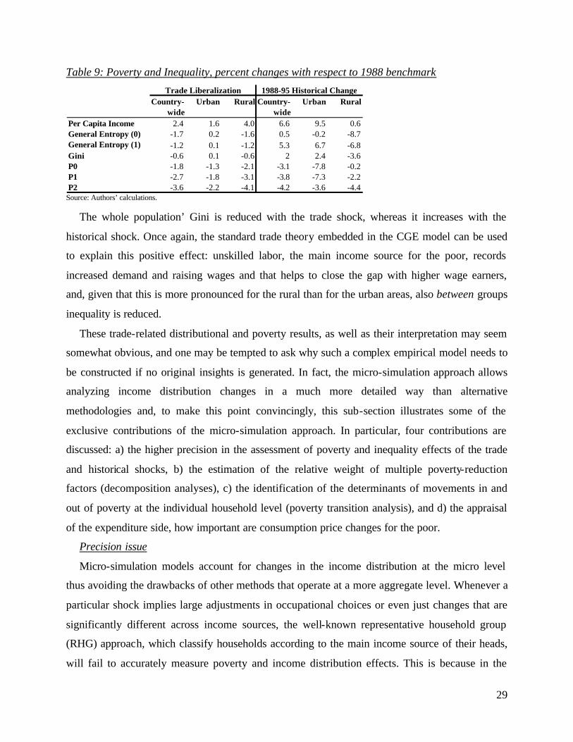
shown in Table 9, a pure trade shock accounts for a large share of overall poverty reduction: for

the whole population the head count (P0) is reduced by 1.8 percent with increased openness,

more than half of the total decrease of 3.1 percent. Trade seems to be particularly beneficial for

the rural poor, given that it reduces the headcount more than in the historical scenario; the reverse

is recorded for the urban poor. This should not be too surprising given that trade liberalization

induces specialization in agricultural exports and other activities requiring rural labor inputs and

that this increased demand is reflected in increased wage and income levels (see Table 8).

Trade also scores well when the poverty severity (P2) index is examined. Even for the urban

areas, trade- induced reduction of P2 is close to the overall historical reduction. This positive

distributional effect is confirmed by looking at inequality indicators.

29

Table 9: Poverty and Inequality, percent changes with respect to 1988 benchmark

Country-wide

Urban Rural Country-wide

Urban Rural

Per Capita Income 2.4 1.6 4.0 6.6 9.5 0.6General Entropy (0) -1.7 0.2 -1.6 0.5 -0.2 -8.7General Entropy (1) -1.2 0.1 -1.2 5.3 6.7 -6.8Gini -0.6 0.1 -0.6 2 2.4 -3.6P0 -1.8 -1.3 -2.1 -3.1 -7.8 -0.2P1 -2.7 -1.8 -3.1 -3.8 -7.3 -2.2P2 -3.6 -2.2 -4.1 -4.2 -3.6 -4.4

Trade Liberalization 1988-95 Historical Change

Source: Authors’ calculations.

The whole population’ Gini is reduced with the trade shock, whereas it increases with the

historical shock. Once again, the standard trade theory embedded in the CGE model can be used

to explain this positive effect: unskilled labor, the main income source for the poor, records

increased demand and raising wages and that helps to close the gap with higher wage earners,

and, given that this is more pronounced for the rural than for the urban areas, also between groups

inequality is reduced.

These trade-related distributional and poverty results, as well as their interpretation may seem

somewhat obvious, and one may be tempted to ask why such a complex empirical model needs to

be constructed if no original insights is generated. In fact, the micro-simulation approach allows

analyzing income distribution changes in a much more detailed way than alternative

methodologies and, to make this point convincingly, this sub-section illustrates some of the

exclusive contributions of the micro-simulation approach. In particular, four contributions are

discussed: a) the higher precision in the assessment of poverty and inequality effects of the trade

and historical shocks, b) the estimation of the relative weight of multiple poverty-reduction

factors (decomposition analyses), c) the identification of the determinants of movements in and

out of poverty at the individual household level (poverty transition analysis), and d) the appraisal

of the expenditure side, how important are consumption price changes for the poor.

Precision issue

Micro-simulation models account for changes in the income distribution at the micro level

thus avoiding the drawbacks of other methods that operate at a more aggregate level. Whenever a

particular shock implies large adjustments in occupational choices or even just changes that are

significantly different across income sources, the well-known representative household group

(RHG) approach, which classify households according to the main income source of their heads,

will fail to accurately measure poverty and income distribution effects. This is because in the

30

RHG method, all households belonging to a particular group are considered identical, and even

when a group’s income is generated across different sources – thus avoiding the extreme case of a

one-to-one income-type-to-household-category mapping – the initial shares across income

sources are fixed. However, in reality not only households heads (or other members) change

occupation and therefore become members of different groups (in a standard RHG method this

‘migration’ is not allowed), but also households within the same group do record heterogeneous

shares of their income sources, so that, for certain shocks, this heterogeneity may determine

whether they escape or not poverty.

A direct comparison between the results obtained using the RHG assumption and those of the

full sample micro-simulation illustrates these precision issues for the Colombian case. It should

be stressed that the RHG method applied here takes into account changes in the occupational

choice of the household heads and so it is quite more flexible than a standard RHG application.

In the case of the trade scenario, as shown in Table 10, the full sample and RHG approaches

produce similar results: changes always show the same sign and are of similar magnitude. The

RHG approach does not account for shifts of spouses (and other non-head household members)

from, say, self-employment in subsistence agriculture to highly paid wage-employment.

However, given that such shifts are of minor importance in the trade scenario, the RHG estimates

are not strongly biased. Besides, in the current trade scenario, both wages of the unskilled and

agricultural profits register similar increases, and the advantages of accounting for full

heterogeneity in sources of income do not matter.

Conversely, important differences between the results of the two methods arise for the

historical simulation. In general, the reasons for these differences are major occupational choice

changes, which significantly altered the composition of household income, and large differences

in the relative gains and losses across labor income sources.

Consider first the differences in poverty indicators. Interestingly, as indicated in Table 10, the

deviations between the two approaches appear to be minor on a countrywide level. Looking at

urban and rural areas separately however reveals that this is coincidental. The reduction of the

poverty gap and the poverty severity index are overestimated under the RHG approach in urban

areas, whereas they are underestimated in rural areas. This demonstrates that the RHG approach

does not introduce a systematic upward or downward bias. The sign of the bias is shock specific.

The RHG’s overestimation of the decrease of the poverty gap and the severity index in urban

areas is due to the large increase of self-employment profits: the entire household income rises by

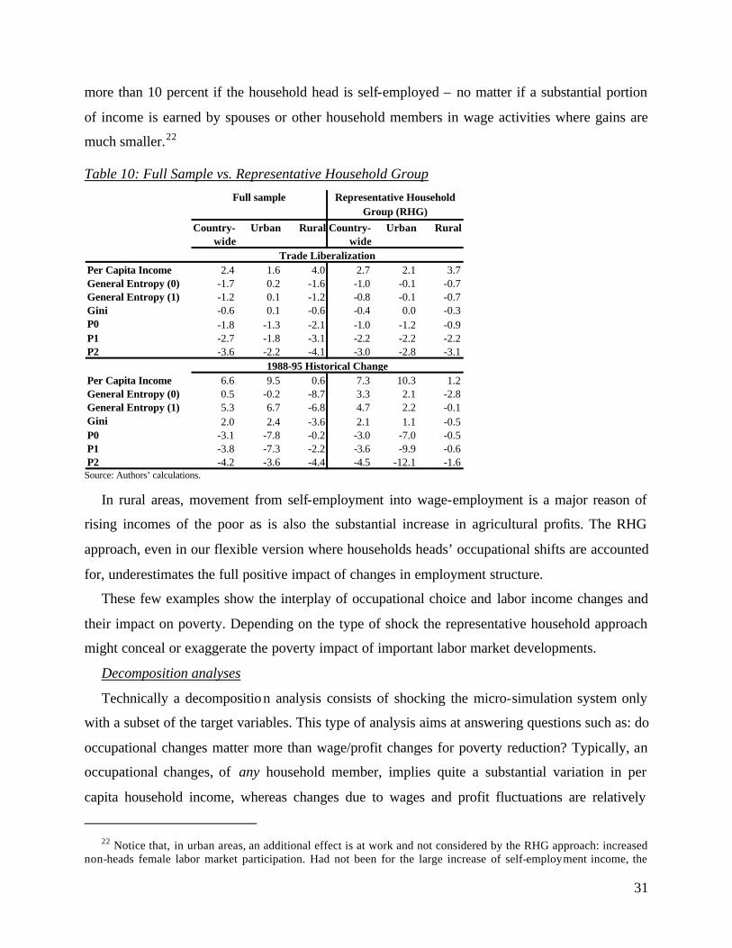
31

more than 10 percent if the household head is self-employed – no matter if a substantial portion

of income is earned by spouses or other household members in wage activities where gains are

much smaller.22

Table 10: Full Sample vs. Representative Household Group

Country-wide


Urban Rural

Per Capita Income 2.4 1.6 4.0 2.7 2.1 3.7General Entropy (0) -1.7 0.2 -1.6 -1.0 -0.1 -0.7General Entropy (1) -1.2 0.1 -1.2 -0.8 -0.1 -0.7Gini -0.6 0.1 -0.6 -0.4 0.0 -0.3P0 -1.8 -1.3 -2.1 -1.0 -1.2 -0.9P1 -2.7 -1.8 -3.1 -2.2 -2.2 -2.2P2 -3.6 -2.2 -4.1 -3.0 -2.8 -3.1

Per Capita Income 6.6 9.5 0.6 7.3 10.3 1.2General Entropy (0) 0.5 -0.2 -8.7 3.3 2.1 -2.8General Entropy (1) 5.3 6.7 -6.8 4.7 2.2 -0.1Gini 2.0 2.4 -3.6 2.1 1.1 -0.5P0 -3.1 -7.8 -0.2 -3.0 -7.0 -0.5P1 -3.8 -7.3 -2.2 -3.6 -9.9 -0.6P2 -4.2 -3.6 -4.4 -4.5 -12.1 -1.6

Full sample Representative Household Group (RHG)

Trade Liberalization

1988-95 Historical Change


In rural areas, movement from self-employment into wage-employment is a major reason of

rising incomes of the poor as is also the substantial increase in agricultural profits. The RHG

approach, even in our flexible version where households heads’ occupational shifts are accounted

for, underestimates the full positive impact of changes in employment structure.

These few examples show the interplay of occupational choice and labor income changes and

their impact on poverty. Depending on the type of shock the representative household approach

might conceal or exaggerate the poverty impact of important labor market developments.

Decomposition analyses

Technically a decomposition analysis consists of shocking the micro-simulation system only

with a subset of the target variables. This type of analysis aims at answering questions such as: do

occupational changes matter more than wage/profit changes for poverty reduction? Typically, an

occupational changes, of any household member, implies quite a substantial variation in per

capita household income, whereas changes due to wages and profit fluctuations are relatively

22 Notice that, in urban areas, an additional effect is at work and not considered by the RHG approach: increased

non-heads female labor market participation. Had not been for the large increase of self-employment income, the

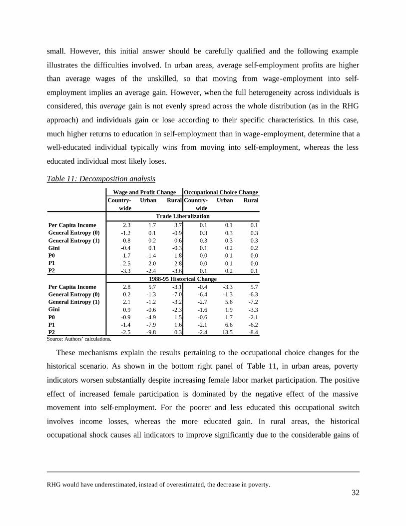
32

small. However, this initial answer should be carefully qualified and the following example

illustrates the difficulties involved. In urban areas, average self-employment profits are higher

than average wages of the unskilled, so that moving from wage-employment into self-

employment implies an average gain. However, when the full heterogeneity across individuals is

considered, this average gain is not evenly spread across the whole distribution (as in the RHG

approach) and individuals gain or lose according to their specific characteristics. In this case,

much higher returns to education in self-employment than in wage-employment, determine that a

well-educated individual typically wins from moving into self-employment, whereas the less

educated individual most likely loses.

Table 11: Decomposition analysis

Country-wide


Urban Rural

Per Capita Income 2.3 1.7 3.7 0.1 0.1 0.1General Entropy (0) -1.2 0.1 -0.9 0.3 0.3 0.3General Entropy (1) -0.8 0.2 -0.6 0.3 0.3 0.3Gini -0.4 0.1 -0.3 0.1 0.2 0.2P0 -1.7 -1.4 -1.8 0.0 0.1 0.0P1 -2.5 -2.0 -2.8 0.0 0.1 0.0P2 -3.3 -2.4 -3.6 0.1 0.2 0.1

Per Capita Income 2.8 5.7 -3.1 -0.4 -3.3 5.7General Entropy (0) 0.2 -1.3 -7.0 -6.4 -1.3 -6.3General Entropy (1) 2.1 -1.2 -3.2 -2.7 5.6 -7.2Gini 0.9 -0.6 -2.3 -1.6 1.9 -3.3P0 -0.9 -4.9 1.5 -0.6 1.7 -2.1P1 -1.4 -7.9 1.6 -2.1 6.6 -6.2P2 -2.5 -9.8 0.3 -2.4 13.5 -8.4



Wage and Profit Change Occupational Choice Change


These mechanisms explain the results pertaining to the occupational choice changes for the

historical scenario. As shown in the bottom right panel of Table 11, in urban areas, poverty

indicators worsen substantially despite increasing female labor market participation. The positive

effect of increased female participation is dominated by the negative effect of the massive

movement into self-employment. For the poorer and less educated this occupational switch

involves income losses, whereas the more educated gain. In rural areas, the historical

occupational shock causes all indicators to improve significantly due to the considerable gains of

RHG would have underestimated, instead of overestimated, the decrease in poverty.

33

moving from agricultural self-employment into wage-employment. The occupational choice

effects dominate the overall impact on the poor.

As far as the trade scenario is considered, a striking feature highlighted in Table 11 is that

almost only change of wage and profit count for the poverty and inequality improvements;

changes of occupational choice seem to be of minor importance. It should also be emphasized

that increased trade openness does not cause the deterioration of rural poverty observed in the

historical scenario, but, on the contrary, trade seems to be quite helpful in reducing poverty in

rural areas due to significant income increases. Additional non-trade-related shocks must then

explain the worsening situation of the rural population in the historical scenario.

Decomposition exercises can be used to analyze the contribution of developments in particular

labor market segments to the overall distributional trends and this may provide valuable insight to

policy makers interested, for example, in the effect of female labor market behavior.

Poverty transition

As explained in section 3.1, the micro-simulation model was modified to allow tracing

individuals through time so that poverty transition analyses could be conducted. One of the main

advantages of these analyses consist of identifying movements in and out of poverty (not only the

net final effect as described in Table 9) so that studying the characteristics of the persistent poor

or understanding which factors help specific individuals escaping poverty becomes possible.

According to their position with respect to the poverty line before and after the shock,

households were grouped in four categories: i) households becoming non-poor, ii) households

falling into poverty, iii) households remaining poor, and iv) households remaining non-poor. The

first three columns of Table 12 show the size of these four categories for the trade liberalization

and historical shock.

It is noticeable that the movements out of poverty of the trade shock are a large proportion of

those caused by the overall shock, but, most importantly, it seems that increased openness

generates less poverty than the overall shock, especially in the rural area. The group of those who

remained poor and especially that of the constantly non-poor show comparable sizes across the

two scenarios. Different characteristics of these groups could be examined and columns 4, 5, 6

and 7 of the table show some preliminary results when the initial distance from the poverty line

and the household’s numbers of active members ratio are considered.

The table’s figures show that, looking at countrywide averages, those escaping from and those

falling into poverty appear to experience similar gains and losses. This is true for both scenarios

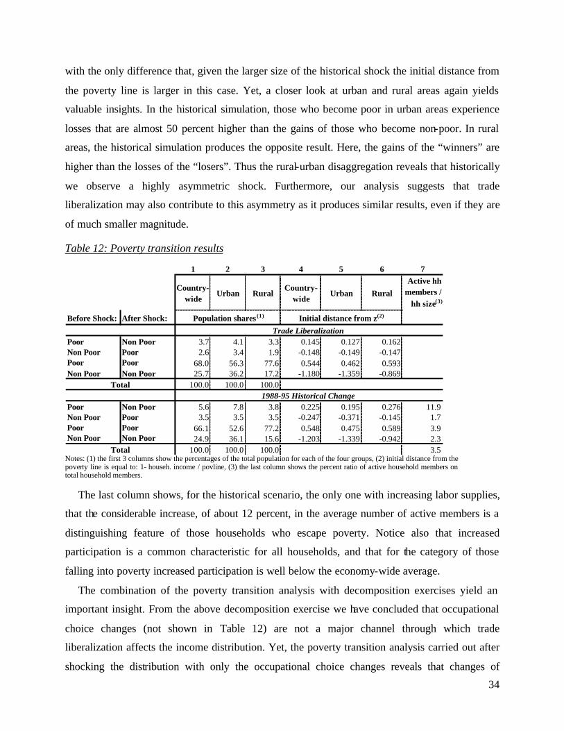
34

with the only difference that, given the larger size of the historical shock the initial distance from

the poverty line is larger in this case. Yet, a closer look at urban and rural areas again yields

valuable insights. In the historical simulation, those who become poor in urban areas experience

losses that are almost 50 percent higher than the gains of those who become non-poor. In rural

areas, the historical simulation produces the opposite result. Here, the gains of the “winners” are

higher than the losses of the “losers”. Thus the rural-urban disaggregation reveals that historically

we observe a highly asymmetric shock. Furthermore, our analysis suggests that trade

liberalization may also contribute to this asymmetry as it produces similar results, even if they are

of much smaller magnitude.

Table 12: Poverty transition results

1 2 3 4 5 6 7

Country-wide

Urban RuralCountry-

wideUrban Rural

Active hh members /

hh size(3)

Before Shock: After Shock:

Poor Non Poor 3.7 4.1 3.3 0.145 0.127 0.162Non Poor Poor 2.6 3.4 1.9 -0.148 -0.149 -0.147Poor Poor 68.0 56.3 77.6 0.544 0.462 0.593Non Poor Non Poor 25.7 36.2 17.2 -1.180 -1.359 -0.869

100.0 100.0 100.0

Poor Non Poor 5.6 7.8 3.8 0.225 0.195 0.276 11.9Non Poor Poor 3.5 3.5 3.5 -0.247 -0.371 -0.145 1.7Poor Poor 66.1 52.6 77.2 0.548 0.475 0.589 3.9Non Poor Non Poor 24.9 36.1 15.6 -1.203 -1.339 -0.942 2.3

100.0 100.0 100.0 3.5

Initial distance from z(2)


1988-95 Historical ChangeTotal

Total

Population shares (1)

Notes: (1) the first 3 columns show the percentages of the total population for each of the four groups, (2) initial distance from the poverty line is equal to: 1- househ. income / povline, (3) the last column shows the percent ratio of active household members on total household members.

The last column shows, for the historical scenario, the only one with increasing labor supplies,

that the considerable increase, of about 12 percent, in the average number of active members is a

distinguishing feature of those households who escape poverty. Notice also that increased

participation is a common characteristic for all households, and that for the category of those

falling into poverty increased participation is well below the economy-wide average.

The combination of the poverty transition analysis with decomposition exercises yield an

important insight. From the above decomposition exercise we have concluded that occupational

choice changes (not shown in Table 12) are not a major channel through which trade

liberalization affects the income distribution. Yet, the poverty transition analysis carried out after

shocking the distribution with only the occupational choice changes reveals that changes of

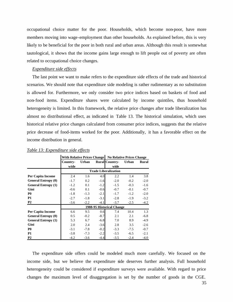
35

occupational choice matter for the poor. Households, which become non-poor, have more

members moving into wage-employment than other households. As explained before, this is very

likely to be beneficial for the poor in both rural and urban areas. Although this result is somewhat

tautological, it shows that the income gains large enough to lift people out of poverty are often

related to occupational choice changes.

Expenditure side effects

The last point we want to make refers to the expenditure side effects of the trade and historical

scenarios. We should note that expenditure side modeling is rather rudimentary as no substitution

is allowed for. Furthermore, we only consider two price indices based on baskets of food and

non-food items. Expenditure shares were calculated by income quintiles, thus household

heterogeneity is limited. In this framework, the relative price changes after trade liberalization has

almost no distributional effect, as indicated in Table 13. The historical simulation, which uses

historical relative price changes calculated from consumer price indices, suggests that the relative

price decrease of food-items worked for the poor. Additionally, it has a favorable effect on the

income distribution in general.

Table 13: Expenditure side effects

Country-wide


Urban Rural

Per Capita Income 2.4 1.6 4.0 2.2 1.4 3.8General Entropy (0) -1.7 0.2 -1.6 -2.0 -0.2 -2.0General Entropy (1) -1.2 0.1 -1.2 -1.5 -0.3 -1.6Gini -0.6 0.1 -0.6 -0.7 -0.1 -0.7P0 -1.8 -1.3 -2.1 -1.7 -1.2 -2.0P1 -2.7 -1.8 -3.1 -2.8 -1.9 -3.2P2 -3.6 -2.2 -4.1 -3.7 -2.5 -4.2

Per Capita Income 6.6 9.5 0.6 7.4 10.4 1.3General Entropy (0) 0.5 -0.2 -8.7 2.1 2.1 -6.8General Entropy (1) 5.3 6.7 -6.8 7.0 8.9 -4.9Gini 2.0 2.4 -3.6 2.8 3.5 -2.6P0 -3.1 -7.8 -0.2 -3.3 -7.5 -0.7P1 -3.8 -7.3 -2.2 -3.5 -6.5 -2.1P2 -4.2 -3.6 -4.4 -3.5 -2.4 -4.0



With Relative Prices Change No Relative Prices Change

The expenditure side offers could be modeled much more carefully. We focused on the

income side, but we believe the expenditure side deserves further analysis. Full household

heterogeneity could be considered if expenditure surveys were available. With regard to price

changes the maximum level of disaggregation is set by the number of goods in the CGE.

36

Furthermore, changes in expend iture shares could be passed from the CGE to the micro-

simulation, or endogenized in the micro-simulation module.

5 Conclusions

This paper employs a novel methodology, pioneered for Indonesia by Robilliard et al (2002),

to study poverty and inequality consequences of trade liberalization, a quintessential globalization

shock. This methodology entails combining in a sequential fashion a numerical simulation

general equilibrium macro model with a micro simulation income distribution model. The former

provides counter factual scenarios and estimates aggregate results, the latter evaluates the poverty

and inequality micro impacts due to these scenarios. This approach overcomes the main difficulty

of single-country case studies based on single year household survey or on multi year surveys

where households cannot be identified through time. Namely our method allows to identify the

income distribution effects due to a particular shock and to estimate the magnitude of these

effects separately from other simultaneous shocks.

When this methodology is applied for Colombia and the particular shock under study is trade

liberalization our main results and policy conclusion can be summarized as follows. Trade

liberalization can substantially contribute to improve the poverty situation. Abstracting from

simultaneous additional shocks and labor supply growth, the beginning of the nineties tariff

abatement seems to have accounted for a very large share of the total reduction in poverty

recorded from 1988 to 1995. This holds in particular for rural areas. Furthermore distributional

impacts differ fundamentally between rural and urban areas. Structural change and the

corresponding occupational choice changes trigger large income gains in particular for the poor.

Generating more wage-employment in formal sectors or increasing female labor market

participation are identified as important sources of higher incomes. Given their diverting

performances, an analysis aggregating rural and urban areas, would only estimate smaller net

effects and potentially mislead policy decisions.

Finally it should also be emphasized that in the case of trade liberalization, the income

channel, i.e. employment status and wage levels, is more important to the poor than the

expenditure channel, i.e. the variation in the price of consumption goods.

37

6 Bibliography

Adelman, I. and S. Robinson (1978), “Income Distribution Policy in Developing Countries: A Case Study of Korea”, New York, Oxford University Press

Alatas, V. and F. Bourguignon (2000), “ The Evolution of the Distribution of Income During Indonesian Fast Growth: 1980-96”, mimeo, Princeton University.

Andersen, L.E. (2000), “Social Mobility in Latin America”, IISEC Working Paper. Armington, P. (1969), “A Theory of Demand for Products Distinguished by Place of

Production”, IMF Staff Papers , Vol. 16, pp. 159-178. Atkinson, A. B., F. Bourguignon, and C. Morrisson (1992), “Empirical Studies of Earnings

Mobility”, Fundamentals of Pure and Applied Economics, 52, Harwood Academic Publishers, Switzerland.

Bussolo M. and D. Roland-Holst. (1999) “Colombia and the NAFTA”, Integration and Trade , September-December 99, INTAL, Washington D.C.

Bussolo M. and R. Correa (1999), “A 1994 Detailed Social Accounting Matrix for Colombia”, Technical Paper no 5, Fedesarrollo. Bogotá, 1999.

Bussolo M., D. Roland-Holst, and D. van der Mensbrugghe (1998), “The Technical Specification of FEDESARROLLO's Long Run General Equilibrium Model” Technical Paper no 4. Fedesarrollo. Bogotá, 1998.

Bussolo M. and J. I. Round (2003), ”Poverty Reduction Strategies in a Budget -Constrained Economy: The Case of Ghana”, Paper presented at the OECD Development Centre Conference on Globalization and Poverty.

Dollar, David and Aart Kraay, (2000), “Trade, Growth, and Poverty”, World Bank Policy Research Working Paper no. 2615.

Goldberg, P. K. and N. Pavcnik (2003), “The Response of the Informal Sector to Trade Liberalization” NBER Working Paper No 9443.

Kugler, A. (1999) “The Impact of Firing Costs on Turnover and Unemployment: Evidence from The Colombian Labour Market Reform”, International Tax and Public Finance Journal, Vol. 6, no. 3, pp. 389-410.

Kugler, A. and M. Cardenas (1999), “The Incidence of Job Security Regulation on Labour Market Flexibility and Compliance in Colombia”, mimeo.

Loefgren, H.; Harris, R. L. and S. Robinson (2001), “ A Standard Computable General Eqilibrium Model in GAMS”, TMD Discussion Paper, No. 75, IFPRI, Washington D.C:.

Newhouse, D. (2001), “Do Negative Income Shocks Last Longer, and Do They Hurt the Poor More? Evidence from Rural Indonesia.”, mimeo, Cornell University.

Núñez, J. A. and J.A. Jiménez (1997), “Correcciones a los Ingresos de la Encuestas de Hogares y Distributcion del IngresoUrbano en Colomia”, mimeo, República de Colombia, Departamento de Planeación.

Ocampo, J.A., F. Sánchez, and C. E. Tovar (2000) “Mercado Laboral y Distribución del Ingreso en Colombia en los Años Noventa”, Revista de la CEPAL, No. 72.

Robilliard, A.-S., F. Bourguignon, and S. Robinson (2002), “Examining the Social Impact of the Indonesian Financial Crisis Using a Micro-Macro Model”, mimeo.

Rodriguez, Francisco and Dani Rodrik (2000), “Trade Policy and Economic Growth: A Skeptic’s Guide to the Cross-National Evidence,” in Ben Bernanke and Kenneth S. Rogoff, eds., NBER Macro Annual 2000, Cambridge, MA: NBER.

Srinivasan, T.N., and Jadgish Bhagwati, (1999), “Outward-Orientation and Development: Are Revisionists Right?” Yale U. mimeo.

38

UNDP (1998), “Informe de Desarrollo Humano para Colombia – 1998”. Vélez, C. E., J. Leibovich, A. Kugler, C. Bouillón, and J. Núñez (2001), “The reversal of

inequality trends in Colombia 1978-1995: A combination of persistent and fluctuating forces”, mimeo, World Bank.

World Bank (2002), “Colombia Poverty Report”.

Globalization and poverty changes in Colombia - World...

Documents

Transcript of Globalization and poverty changes in Colombia - World...