Global VSAT Forumold.gvf.org/approvals/images/pdf/typeapprovalsdoc/GVF... · 2019-05-04 · Global...

Global VSAT Forum

GVF-105 Rev 8

Global VSAT Forum PERFORMANCE AND TEST GUIDELINES FOR TYPE APPROVAL OF 'COMMS ON THE MOVE' MOBILE SATELLITE COMMUNICATIONS TERMINALS Released document.

GVF-105

This document defines the applicable performance requirements and test procedures for GVF Type Approval of "Comms on the Move" mobile satellite communications antenna systems. Revision History: Document Status Notes GVF105 Released Original Document (Tim Shroyer 08/09)

Revised Document (Colin Robinson 02/11) Revised Document (Rami Adada 12/12) Revised Document (Tim Shroyer 04/13) Revised Document (Rami Adada 05/13) Revised Document (Rami Adada & Colin Robinson 07/13) Released Document (Rami Adada 08/13) Revised Document (Markus Landmann, Mostafa Alazab, Colin Robinson 01/16)

Global VSAT Forum

GVF-105 Rev 8

TableofContents 1 Purpose .................................................................................................................................... 32 Terminal Definition ................................................................................................................... 3

3 Background .............................................................................................................................. 3

4 Reference Performance Requirements .................................................................................... 4

4.1 ETSI EN 302 977 (Ku-Band COTM) ................................................................................. 44.2 FCC 25.226 (Ku-Band COTM) .......................................................................................... 54.3 On-Satellite Cross-Pol EIRPSD Limit References ............................................................ 64.4 Antenna Radiation Pattern Limit Reference ...................................................................... 6

5 Type Approval Test Requirements ........................................................................................... 6

5.1 Pre-defined parameters .................................................................................................... 75.2 Required Tests .................................................................................................................. 85.3 Test Methods .................................................................................................................... 8

5.3.1 Pointing Accuracy Testing of Terminals with Small Antennas (ie. ≤ ~ 0.8m Diameter at Ku-Band) .............................................................................................................................. 85.3.2 Verification testing of the “Transmit Inhibit” function ................................................ 115.3.3 Verification testing of the level of Cross-Pol interference that the terminal emits towards the desired satellite under normal operating conditions ........................................... 125.3.4 Verification testing of antenna "skew" corrections for non-circular apertures .......... 145.3.5 Motion Profile Definition for verification of pointing accuracy, cross pol, skew correction ............................................................................................................................... 16

Appendices .................................................................................................................................... 30Appendix A: Additional Notes on Pointing Accuracy Verification Method ..................................... 31

Appendix B: The Faciltiy for Over-the-air Research and Testing FORTE at Fraunhofer IIS ......... 43

Appendix C: Additional Notes on Standard Motion Profiles .......................................................... 57

Appendix D: Literature .................................................................................................................. 77

Appendix E: List of acronyms ........................................................................................................ 78

Global VSAT Forum

GVF-105 Rev 8

1 Purpose The GVF type approval process is defined in detail in document GVF-101. This document adds guidance for testing parameters that are unique to COTM terminals. These include the terminal tracking accuracy and the up-link inhibit functions should the tracking accuracy exceed published specifications. This testing is in addition to the test requirements outlined in GVF-101 [Mutual Recognition of Performance Measurement Guidelines and Procedures for Satellite System Operator Type approvals].

2 Terminal Definition A COTM terminal is defined for the purposes of this document as follows:

1) C, X, Ku or Ka-Band operation.

2) Intended for operation on geostationary (non-inclined) satellites.

3) Automatically deploys, and accurately points, its antenna towards a designated target satellite.

4) Fully stabilized and suitable for vessels and moving vehicles.

5) Either (1) operates as part of a managed network, in which there is a hub or other

counterpart earth station that is required for the terminal to operate and which supports terminal operations, or (2) operates as a standalone uplink station and all control functions are self-contained.

6) The type approval is granted to an agreed unique configuration, comprising the antenna (identified by manufacturer, model and diameter), mount, antenna control system, RF chain and modem. The maximum allowed EIRP density will be defined on the basis of the antenna RF performance and the results of the auto-deploy tests. The existing communication between modem and the platform shall be described by the manufacturer e.g. presence of power control in the modem, modem locking signal characteristics etc. In case of a different type of modem replacing the one of the originally type approved configuration, additional test plans will have to be mutually agreed between the applicant and the ATE (Authorized test Entity). If the manufacturer demonstrates that the pointing and RF parameters are not subject to a high level of modem dependency, other types of modems can be validated by analysis only.

3 Background COTM applications place severe restrictions on the size of the antenna used as profile drag and limited footprint are key design elements for vehicles where these terminals are mounted. In many cases, this entails the use of Ultra Small Aperture Terminals (USATs) (i.e. < 1.0m at Ku-Band) that are inherently restricted in their focusing ability and thus produce wider beams. The combination of these wider beams with the increase risk of miss-pointing, due to the dynamic nature of the platform these terminals are mounted on, makes it critical to ensure that these terminals don’t cause excessive levels of interference.

For example, with respect to Vehicle Mounted Earth Stations (VMES), ETSI EN 302 977 and FCC 25.226 address the issue of adjacent satellite interference by imposing limits on the levels of

Global VSAT Forum

GVF-105 Rev 8

off-axis emissions produced by the COTM terminal as well as requiring the terminal to inhibit transmission when a pointing error exceeding the manufacturer’s declared threshold occurs as this would imply that the off-axis emissions limits are possibly being exceeded by the terminal if transmission is uninhibited. ETSI EN 302 977 also addresses the issue of on satellite cross-polarization interference that linearly polarized COTM terminals may cause due to tracking error on the antenna’s transmit polarization axis.

These however don’t provide test methodologies to verify compliance. It is therefore the intent of this document to present test methods, for conditions unique to COTM terminals that would be required in addition to the general VSAT test requirements outlined in GVF-101.

4 Reference Performance Requirements For VMES, specifications such as ETSI EN 302 977, FCC 25.226 and ITU-R S.1857 exist. For Earth Stations on Trains (EST) at Ku-Band, ETSI EN 302 448 is defined. For Earth Stations on Vessels (ESV) or Aircraft Earth Stations (AES), other specifications exist. For example, ETSI EN 302 340 and FCC 25.222 are specified for ESVs at Ku-Band. ETSI EN 302 186 and FCC.222 are specified for AESs at Ku-Band. At Ka-Band, ETSI EN 303 978 and FCC 25.138 are specified for all types of Earth Stations On Mobile Platforms (ESOMP). As an example, the ETSI EN 302 977 and the FCC 25.226 norms for VMES at Ku-Band are discussed below. It is important to note that some satellite operators may require additional/different performance specifications.

4.1 ETSI EN 302 977 (Ku-Band COTM) Off-Axis EIRP Spectral Density Limits: • Co-Pol:

• 33 - 25 log (φ + δφ) - H dBW/40KHz for 2,5 ° ≤ φ + δφ ≤ 7,0 °

• 12 - H dBW/40KHz for 7,0 ° < φ + δφ ≤ 9,2 °

• 36 - 25 log (φ + δφ) - H dBW/40KHz for 9,2 ° < φ + δφ ≤ 48 °

• - 6 - H dBW/40KHz for φ + δφ > 48 °

• Cross-Pol:

• 23 - 25 log (φ + δφ) - H dBW/40KHz for 2,5 ° ≤ φ + δφ ≤ 7,0 °

• 2 - H dBW/40KHz for 7,0 ° < φ + δφ ≤ 9,2 °

Notes: • φ is the angle, in degrees, between the main beam axis and the direction considered

• δφ is the pointing error threshold, in degrees, as declared by the applicant

• H (in dB) is 10logN where N is the maximum number of VMESs which may transmit in the same

carrier frequency band as declared by the applicant.

•The radiation pattern planes for which these restrictions apply can be limited if documentary

evidence is provided that not all directions are concerned. TR 102 375 gives guidance on

determination of the concerned subset.

Global VSAT Forum

GVF-105 Rev 8

Pointing Error and Cessation of Emissions: • The maximum pointing error requirement is to be set by the applicant as long as the terminal

meets their off-axis EIRP spectral density limits when mispointed by this value.

• The terminal shall cease transmission if the maximum pointing error is exceeded for a period

of T seconds (T is set by the applicant).

• The terminal will not restart transmission unless the pointing error is within the limit for a

period of 2xT seconds.

• T is not to exceed 2 seconds

4.2 FCC 25.226 (Ku-Band COTM) Off-Axis EIRP Spectral Density Limits: • Co-Pol in the GSO plane:

• 15–10log(N)–25logΘ dBW/4kHz for 1.5° ≤ Θ ≤ 7°

• −6 −10log(N) dBW/4kHz for 7° < Θ ≤ 9.2°

• 18 −10log(N)–25logΘ dBW/4kHz for 9.2° < Θ ≤ 48°

• −24 −10log(N) dBW/4kHz for 48° < Θ ≤ 85°

• −14 −10log(N) dBW/4kHz for 85° < Θ ≤ 180°

For Θ > 7° the envelope can be exceeded by up to 10% of the sidelobes by a maximum of 3dB • Co-Pol in all other planes:

• 18−10log(N)−25logΘ dBW/4kHz for 3.0° ≤ Θ ≤ 48°

• −24−10log(N) dBW/4kHz for 48° < Θ ≤ 85°

• −14−10log(N) dBW/4kHz for 85° < Θ ≤ 180°

Envelope can be exceeded by up to 10% of the sidelobes by a maximum of 6dB • Cross Pol:

• 5−10log(N)−25logΘ dBW/4kHz for 1.8° ≤ Θ ≤ 7.0°

• −16−10log(N) dBW/4kHz for 7.0° < Θ ≤ 9.2°

Pointing Error and Cessation of Emissions: • Requires compliance to one of the following 2 conditions regarding maximum pointing error,

each of which has a specific cessation of emission requirement:

A. Maximum pointing error ≤ 0.2°

• Cessation of emission occurs within 100 msec if pointing error

exceeds 0.5°

• Transmission to resume when pointing error ≤ 0.2°

Global VSAT Forum

GVF-105 Rev 8

Or

B. Determined by the applicant based on the terminal still meeting the FCC off-axis

EIRP density limits when mispointed by this value (Similar to the ETSI definition)

• Cessation of emissions occurs within 100 msec if pointing error

exceeds specified pointing error threshold

• Transmission to resume when pointing error is below threshold

4.3 On-Satellite Cross-Pol EIRPSD Limit References Within the stated pointing error threshold of the terminal, the EIRPSD of the cross-polarized signal should not exceed:

• For Ku-Band Terminals:

o 0 dBW/4KHz (Equivalent to a 1.2m antenna compliant with FCC 25.209 and FCC 25.218 for digital Ku-Band earth-station operation, having an on satellite Cross-Pol isolation of 30dB).

o 8 dBW/4KHz (Equivalent to a 1.2m antenna compliant with FCC 25.209 and ITU-R S.728-1, having an on satellite Cross-Pol isolation of 30dB).

4.4 Antenna Radiation Pattern Limit Reference In addition to the limit on EIRPSD, some satellite operators may require a limit on the antenna gain radiation pattern. One such limit can be found in ITU-R S.465-6 summarized below: • Gain ≤ 32–25logΘ dBi for Θmin ≤ Θ ≤ 7° Where: Θmin = 1° or 100 λ/D degrees, whichever is the greater, for D/λ ≥ 50. Θmin = 2° or 114 (D/λ)–1.09 degrees, whichever is the greater, for D/λ < 50. It should be noted that for non-rotationally symmetric apertures, D is the dimension of the aperture along the plane of the antenna radiation pattern being assessed.

5 Type Approval Test Requirements Type approval for COTM terminals shall include the following provisions:

a) COTM Terminals employing Traditional VSAT antennas: Antennas included in this classification shall be tested per the requirements of this document [GVF-105] and GVF-101 in general and section 4 of GVF-101 in particular.

b) COTM Terminals employing ESA technology or other solutions in which the antenna performance (pattern, gain, polarization and G/T) changes as the antenna pattern is scanned off axis: COTM terminals falling in this classification require special test procedures in addition to the requirements of this document [GVF-105]. This is because of the volume of test measurements that would otherwise have to be undertaken if standard measurement

Global VSAT Forum

GVF-105 Rev 8

procedures were employed. In summary, the pattern characteristics of any COTM terminal falling in to this grouping shall include the following elements. These procedures are outlined in section 4.4 of GVF-101. [GVF-101 is being updated to include Sect 4.4 as an addition.]

1) Provide predicted, principal plane, co- and cross pol antenna pattern coverage plots at the lower, mid and upper frequencies in the transmit and receive bands of interest.

2) Conduct physical antenna pattern measurements corresponding to the pattern predictions for the step (1) above.

3) Compare predicted vs. measured pattern coverage to validate the accuracy of the pattern prediction software.

4) Use the pattern prediction software to identify other regions where specification violations may occur or for areas with minimal performance margins.

5) Conduct physical pattern measurements over the same angular and skew angle regions identified in step (4) above.

The rationale for this approach is simple. First, the accuracy of the prediction software requires validation by comparing predicted performance against measured performance. Second, having established the accuracy of the predicted performance, the process moves to characterize the actual antenna performance for conditions where the predictions indicate areas of risk or non-compliance.

c) COTM Terminals employing Radomes: Radomes can degrade the performance of the

antenna being protected by the radome. The provisions of GVF-105 and GVF-101 shall require that any terminal [COTM, Auto-Deploy or Stationary terminal] normally supplied with a radome as part of its Bill or Materials, be characterized with the radome in place. The radome shall be positioned with respect to the terminal antenna as would be encountered in normal terminal operation. This provision shall apply to all antennas falling on the classifications of paragraphs a) and b) above.

5.1 Pre-defined parameters The manufacturer or type approval applicant must propose the following parameters:

1) Maximum BPE under normal operating conditions†.

2) The length of time T that when the BPE defined above is exceeded for will cause a cessation of emission.

3) For linearly polarized terminals, the cross-pol isolation within the BPE of the terminal.

4) Measured antenna radiation patterns for both Co and Cross polarized components showing an angular range of +/- 7° from bore-sight with a resolution better than 0.1°:

a. For circular aperture antennas these should include 2 orthogonal cuts (e.g. AZ and EL) for 2 orthogonal polarization settings (e.g. Vertical and Horizontal)

b. For elliptical apertures these should include 19 cuts, starting with the AZ cut (i.e. 0° skew cut) going thru to the EL cut (i.e. 90° skew cut) in 5° increments. It is important to note that the maximum compliant on-axis EIRPSD for COTM terminals with non-aligning elliptical aperture antennas will depend on the skew angle of the operating scenario (See appendix for example).

Global VSAT Forum

GVF-105 Rev 8

5.2 Required Tests In addition to testing defined in GVF-101 (VSAT level), COTM terminal testing should include:

• The verification that the manufacturer’s stated pointing error threshold is not exceeded under normal operating conditions†.

• The verification of the “transmit inhibit” function when the stated pointing error threshold is exceeded for the stated time T.

• The verification of the level of Cross-Pol interference that the terminal emits towards the desired satellite under normal operating conditions†.

• The verification of antenna pattern "skew" corrections for non-circular apertures. †Normal operating conditions are minimum profiles to be agreed upon between the terminal manufacturer and the approved GVF test entity based on the target customer application for the terminal. A description of these profiles is to be included in the type approval certificate.

These tests, in combination with the terminal’s radiation pattern measurement (per GVF-101) will allow for determination of a maximum compliant level of on-axis EIRP density for the terminal as shown in Figure 1.

Figure 1: Determination of maximum compliant on-axis EIRP density

5.3 Test Methods

5.3.1 Pointing Accuracy Testing of Terminals with Small Antennas (ie. ≤ ~ 0.8m Diameter at Ku-Band)

Typically, for terminals with large antennas where gain of the main lobe quickly varies away from boresight, pointing accuracy can be accurately determined by monitoring the signal level received by the target satellite since fluctuation of this signal is dominated by changes in pointing error.

Global VSAT Forum

GVF-105 Rev 8

When dealing with terminals with small apertures, as is the case for many COTM terminals, the signal fluctuation at the target satellite caused by pointing error becomes very small, due to the beam flatness near the beam peak, making accurate measurement of pointing error impractical using this approach. The alternative herein described utilizes the fact that these small antennas have a radiation pattern main lobe that is wide enough to be detected at an adjacent satellite providing signal levels suited for calibrated measurements. Essentially, a signal is uplinked to the primary satellite of interest and the downlink signal is simultaneously monitored on both the primary and adjacent satellites. The COTM VSAT terminal is then driven over a course, suggested by the manufacturer and agreed upon by the GVF test entity, which will be representative of typical use of the terminal. The COTM VSAT terminal can equally be installed on a motion table set up to replicate movement of the vehicle. When monitoring the downlink signal on the primary satellite, very small (and often hard-to-detect) changes in received strength may be seen due to small pointing errors as the terminal antenna attempts to compensate for vehicle motion. However, the changes in signal strength recorded on the adjacent satellite downlink will be amplified due to the rapidly changing gain for small angular errors. Once differences between propagation paths (SFD, Receiving aperture G/T …) have been corrected for, the difference between both measured signals referred to as Δ will correspond to the antenna radiation pattern. Since the adjacent satellite is around 2 degrees offset from the beam peak this Δ is quite sensitive to pointing error. Δ (dB) = Measured received signal from adjacent satellite - Measured received signal from desired satellite + Correction Factor Given linear operation of the Terminal under Test, the link via the primary satellite of interest, and the adjacent satellite, it can be shown that the following relationships exist: Prcv Sat1 = Pup Sat1 - Lup Sat1 + GSat1 - LdownSat1 + GMon ET1 and Prcv Sat2 = Pup Sat2 - Lup Sat2 + GSat2 - LdownSat2 + GMon ET2 Where: Prcv Satx =Power received from Satellite x, either primary(1) or adjacent(2) Pup Satx = Power uplinked from Terminal Under Test towards Satellite x Lup Satx = Uplink loss from Terminal Under Test towards Satellite x GSatx = Gain through Satellite x transponder Ldown Satx = Downlink loss from Terminal Under Test towards Satellite x GMon ETx = Gain through Measurement Earth Terminal x With linear operation of links via the primary and adjacent satellites during the period of measurement, the Correction Factor can combine the individual Loss and Gain terms into one factor. If the Correction Factor is time varying, it might still be possible to combine into one term, but with added measurement complexity. Correction Factor can be calculated by determining that value for which: Fcorrection = Prcv Sat1 - Prcv Sat2 - Gup TUT at spacing Where: Fcorrection = Correction Factor Gup TUT at spacing = Gain difference in uplink antenna pattern of Terminal Under Test at the offset angle of the orbital spacing of Satellite 1 and Satellite 2.

Global VSAT Forum

GVF-105 Rev 8

An example of a radiation pattern of a terminal under test along the GSO arc is shown in Figure 2. It can be seen that when the pointing error is 0°, a Δ = -16.7dB should be measured. When a pointing error of 0.5° towards the adjacent satellite occurs, an increase to Δ = -8.2dB will be recorded.

Figure 2: Typical Radiation pattern for COTM terminal with small antenna

The correction factor can be obtained while the terminal is static, by manually peaking the antenna using the -6dB points. The difference between the expected Δ (obtained from the radiation pattern and knowledge of the adjacent satellites relative position with respect to bore-sight) and the measured one while the terminal under test is peaked corresponds to the correction factor. The essential element of this Test Plan is to operate a mobile VSAT terminal under controlled conditions such that:

- Mobile VSAT transmit antenna input power spectral density is maintained as constant as possible.

- Calibrated measurements are made simultaneously on the downlink power spectral

density of the desired satellite and the downlink power spectral density of the adjacent satellite or satellites.

Assuming that the entire satellite communications link remains within the linear region on both the satellite of interest and the adjacent satellites, any impact on EIRP spectral density will result in a direct dB for dB downlink spectral density change. Simultaneous measurements of the downlink spectral density from each of the satellites should result in data which can then be converted from EIRP spectral density to antenna angular offsets. It is that principle which forms the basis of the Test Plan presented here.

Global VSAT Forum

GVF-105 Rev 8

The details of the test procedure may be adapted to accommodate a particular terminal configuration, however "live" on-air test presents an effective method to accurately determine the pointing accuracy for a VSAT terminal when in motion. Using this approach, the pointing accuracy stated by the manufacturer can be verified thru several trials where the terminal is operated under conditions mimicking standard user operation. A typical processed data capture from such a trial is shown in Figure 3.

Figure 3: Typical processed data plot of a trial of the pointing accuracy verification

5.3.2 Verification testing of the “Transmit Inhibit” function Using the same method of measuring pointing accuracy described in 5.3.1, it is possible to verify the transmit inhibit parameters (pointing error threshold and time T) stated by the manufacturer by repeatedly inducing a pointing error that exceeds the error threshold for a period longer than T. Figure 4 shows a typical processed data capture of this testing. In this case, the system inhibits transmit when a pointing error threshold of 0.5° is exceeded for >100ms. As can be seen, when the system is muted, Δ goes to ~ 0dB (this is not exactly 0 because of the noisiness of the measured signal when the terminal is muted).

Global VSAT Forum

GVF-105 Rev 8

Figure 4: Typical processed data plot of a profile used for transmit inhibit verification

5.3.3 Verification testing of the level of Cross-Pol interference that the terminal emits towards the desired satellite under normal operating conditions

The purpose of this test is to verify the level of Cross-Pol interference emitted by the terminal towards the desired satellite under normal operating conditions relative to the peak Co-Pol signal level that can be seen on the desired satellite for the same terminal settings and EIRP level. The test should be conducted in under clear sky conditions. The test starts by manually (i.e. using a “jog” type function on the controller) peaking the terminal by finding the -6dB points. Next transmission from the terminal under test is established. The Co-Pol signal received by the desired satellite is monitored by the hub station for a few minutes. The maximum received signal level is recorded. The COTM terminal is then operated under the agreed upon operating profiles while the hub station is monitoring the Cross-Pol level recorded. Figure 5 shows a typical processed data capture of this testing.

Global VSAT Forum

GVF-105 Rev 8

Figure 5: Typical processed data plot of a profile used for Cross-Pol Interference level testing.

Global VSAT Forum

GVF-105 Rev 8

5.3.4 Verification testing of antenna "skew" corrections for non-circular apertures

COTM terminals can utilize antenna apertures having circular or non-circular radiation patterns. Circular apertures exhibit radiation patterns which are essentially equal in all directions away from the center of the beam. Non-circular apertures, elliptical or other shapes, exhibit narrower effective beamwidths along the longest axis of the aperture. They exhibit wider effective beamwidths along the narrowest axis. This results in a "skew" of non-circular radiation patterns along the geostationary arc which must be considered as it relates to ASI. An example of the definition of antenna radiation pattern "skew", using a rectangular aperture radiation pattern, is provided in Figure 6.

Figure 6: Non-circular antenna aperture radiation pattern "Skew". COTM terminal antenna pattern "skew" will be present in terminals utilizing non-circular apertures. The effects of antenna radiation pattern Skew can be compensated with one of three methods:

1) Establish the COTM terminal's EIRP power spectral density at a level which will satisfy the ASI requirements and radiation in directions other than the geostationary arc under the worst condition.

• Terminals employing this method require no skew angle compensation testing.

2) Establish the COTM terminal's EIRP power spectral density at a level which is intended to satisfy ASI requirements and radiation in directions other than the geostationary arc up to a defined maximum skew angle, and for higher Skew angles to mute the COTM transmitter.

• Terminals employing this method require verification testing of this mute functionality. This can be performed using the following procedure:

Global VSAT Forum

GVF-105 Rev 8

a. Mount a 2 axis inclinometer on the azimuth rotating part of the antenna while aligning one axis such as it is parallel to the elevation axis (Pitch) and the other parallel to the beam direction if the antenna were pointed at 0° elevation (roll).

b. Mount the terminal to a base.

c. Acquire a satellite that is within the terminal’s allowable skew range but close to

the manufacturer’s maximum stated value.

d. While monitoring the RF input power of the antenna (using BUC M&C function or a coupler…), gradually tilt the base to which the terminal is mounted until the antenna RF input power is seen to drop to the noise floor of the test setup.

e. Note the Pitch and Roll values at which the transmission was muted.

f. Using the following equations from [1] (where Pol corresponds to skew) calculate

the corresponding skew of the tilted antenna at which transmission was muted and compare with the manufacturer’s stated value:

Where:

3) Dynamically adjust the COTM terminal's EIRP power spectral density using a determination of the radiation patterns Skew along the geostationary arc, where it affects ASI, and in directions other than the geostationary arc as defined in regulatory requirements.

• Terminals employing this method require verification testing of this functionality. This can be performed using the following procedure:

a. Mount a 2 axis inclinometer on the azimuth rotating part of the antenna while aligning one axis such as it is parallel to the elevation axis (Pitch) and the other parallel to the beam direction if the antenna were pointed at 0° elevation (roll).

b. Mount the terminal to a level base.

c. Acquire a satellite and set the antenna’s input PSD to within 1 dB of the

allowable limit for the corresponding location/satellite combination.

d. Tilt the base so as to increase the terminal skew.

e. Note the input PSD to the antenna at the new terminal skew.

f. Using the above equations from [1] (where Pol corresponds to skew) calculate the corresponding skew of the tilted antenna.

g. Compare the on-axis EIRP density of the tilted terminal to the corresponding

Skew specific EIRP density value specified by the manufacturer.

Global VSAT Forum

GVF-105 Rev 8

Other potential verification test methodologies could be utilized to verify the radiation pattern skew compensation process, subject to minimum profiles to be agreed upon between the terminal manufacturer and the approved GVF test entity based on the target customer application for the terminal. Using any methodology, results of verification tests and any imposed operational constraints of antenna skew compensation should be documented for COTM terminals utilizing non-circular antenna apertures

5.3.5 Motion Profile Definition for verification of pointing accuracy, cross pol, skew correction

In order to offer a fair basis of comparison for different COTM systems, the motion profiles over which the system test is performed have to be defined. The approach here is to define different Classes of equipment in each environment (land mobile, maritime, aeronautic, train). The applicant has to decide on which Class the equipment has to be tested. A successful test under the most challenging class would give automatically an approval for all lower classes. If the test with a higher class fails the test on a lower class could be performed if the applicant agrees. The classes for land mobile and maritime are derived based on the results of an extensive measurement campaign that was performed by Fraunhofer IIS under the ESA Contract: 4000103870/11/NL/NR (under the ESA ARTES 5.1). For the mentioned environments different terrain types and platforms are measured and a database was populated with the motion dynamics of each measurement.

5.3.5.1 Land mobile motion profile definition With respect to the Land Mobile environment, the statistical analysis of the measured data shows two main classes. Class A which include the data with harsh motion dynamics and Class B with lower motion dynamics. Roughly speaking Class A contains harsh terrains as Off-road and Class B covers paved surfaces and relaxed Off-road conditions. Table 1 lists the 95% percentile values (Q95) for the motion dynamics of the two classes. For each parameter the average value over all measurements of Class A & B and the standard deviation are listed.

Parameter Class A Class B Angular Rate [°/s] 29 ± 6 10 ± 6 Angular Acceleration [°/s2] 368 ± 188 242 ± 205 Translational Acceleration [m/s2] 5 ± 2 3 ± 2

Table 1 The Q95 statistics of Class A and Class B for the Land Mobile environment

For each class, one measurement is selected as the standard motion profile for this class. In Appendix B, the detailed selection process is explained. The statistics in terms of the Cumulative Distribution Function (CDF) of the two standard profiles are show in Figure 7 and Figure 8 for the vector norm of the angular rate and the angular acceleration, respectively. The statistics of the well-known ChurchVilleB track are also plotted for comparison.

Global VSAT Forum

GVF-105 Rev 8

Figure 7 CDFs of angular rate vector norm of Class A, Class B and ChurchVilleB tracks

Figure 8 CDFs of angular acceleration vector norm of Class A, Class B and ChurchVilleB tracks

Global VSAT Forum

GVF-105 Rev 8

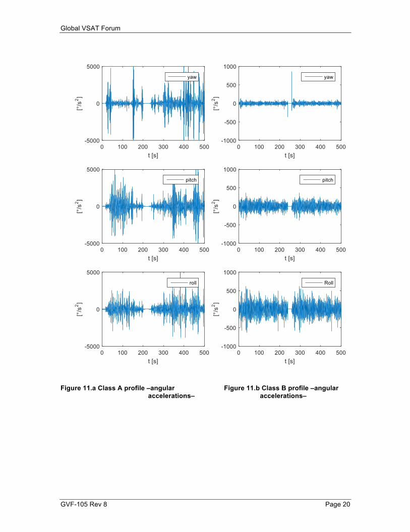
The time series of the standard motion profiles The time series of the motion profiles from Class A and Class B are depicted in Figures 9, 10, 11 and 12 for the angles, angular rates, angular accelerations and translational accelerations, respectively.

Figure 9.a Class A profile –angles– Figure 9.b Class B profile –angles–

Global VSAT Forum

GVF-105 Rev 8

Figure 10.a Class A profile –angular rates– Figure 10.b Class B profile –angular rates–

Global VSAT Forum

GVF-105 Rev 8

Figure 11.a Class A profile –angular Figure 11.b Class B profile –angular accelerations– accelerations–

Global VSAT Forum

GVF-105 Rev 8

Figure 12.a Class A profile –translational Figure 12.b Class B profile

accelerations– –translational accelerations–

The motion profiles can be downloaded from the ESA Database [3]

Global VSAT Forum

GVF-105 Rev 8

5.3.5.2 Maritime motion profile definition With respect to the Maritime environment, the statistical analysis of the measured data shows again two main classes. Class A which include the scenarios with high motion dynamics and Class B with lower motion dynamics. Table 2 lists the 95% percentile values (Q95) for the motion dynamics of the two classes. For each parameter the average value over all measurements of Class A & B and the standard deviation are listed.

Parameter Class A Class B Angular Rate [°/s] 14 ± 3 1.5 ± 2 Angular Acceleration [°/s2] 222 ± 170 16 ± 20 Translational Acceleration [m/s2] 4 ± 1 0.6 ± 0.6

Table 2 The Q95 statistics of Class A and Class B for the Maritime environment

For each class, one measurement is selected as the standard motion profile for this class. In Appendix B, the detailed selection process is explained. The statistics in terms of the Cumulative Distribution Function (CDF) of the two Maritime standard profiles are shown in Figure 13 and Figure 14 for the vector norm of the angular rate and the angular acceleration, respectively.

Figure 13: CDFs of angular rate vector norm of Class A, Class B tracks

Global VSAT Forum

GVF-105 Rev 8

Figure 14: CDFs of angular acceleration vector norm of Class A, Class B tracks

Global VSAT Forum

GVF-105 Rev 8

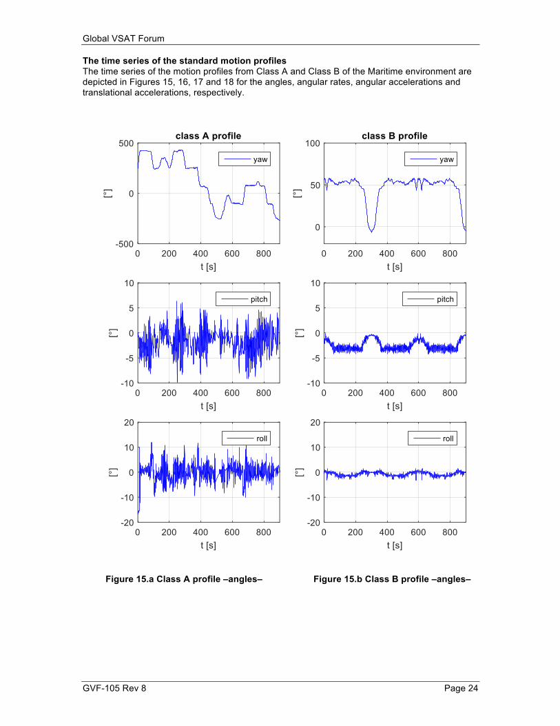
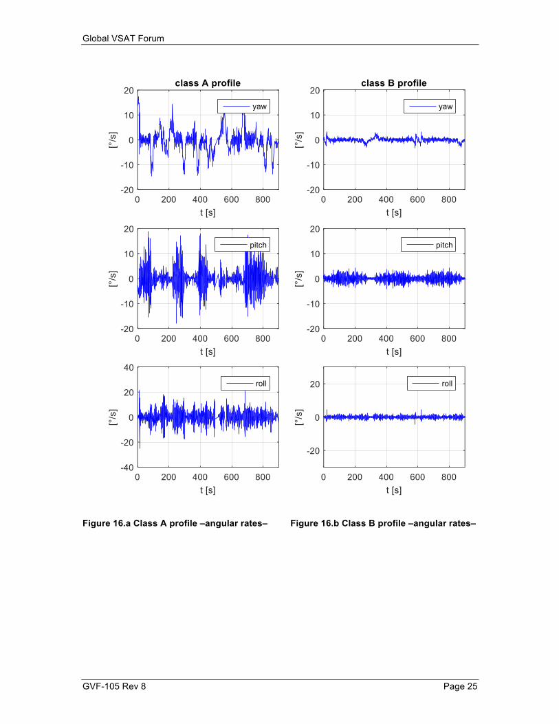
The time series of the standard motion profiles The time series of the motion profiles from Class A and Class B of the Maritime environment are depicted in Figures 15, 16, 17 and 18 for the angles, angular rates, angular accelerations and translational accelerations, respectively.

Figure 15.a Class A profile –angles– Figure 15.b Class B profile –angles–

Global VSAT Forum

GVF-105 Rev 8

Figure 16.a Class A profile –angular rates– Figure 16.b Class B profile –angular rates–

Global VSAT Forum

GVF-105 Rev 8

Figure 17.a Class A profile –angular Figure 17.b Class B profile –angular accelerations– accelerations–

Global VSAT Forum

GVF-105 Rev 8

Figure 18.a Class A profile –translational Figure 18.b Class B profile

accelerations– –translational accelerations–

The motion profiles can be downloaded from the ESA Database [3]

Global VSAT Forum

GVF-105 Rev 8

5.3.5.3 Comparison of the Land mobile and maritime standard profiles The CDFs of the standard motion profiles are plotted in Figure 19 and Figure 20 along with the CDF of the land mobile motion profiles. The CDFs are plotted w.r.t. the vector norm of the angular rate and angular acceleration. It can be see that the land mobile class A represents the upper bound of the motion dynamics and the Maritime class B represents the lower bound. The land mobile class B and the Maritime class A tracks are in the middle.

Figure 19 CDFs of angular rate vector norm of the Land mobile as well as the Maritime

selected profiles

Global VSAT Forum

GVF-105 Rev 8

Figure 20 CDFs of angular acceleration vector norm of the Land mobile as well as the Maritime selected profiles

5.3.5.4 Application of motion profiles in Type Approval A COTM terminal can be approved either in: 1. A laboratory environment where the dynamics and the actual time series of the motion profiles from Class A and Class B can be replayed and the tracking performance in terms of de-pointing and/or off axis EIRP can be measured. One of these facilities is the Facility for Over-the-air Research and Testing (FORTE [3,4]) which is built and operated by the Fraunhofer IIS in Germany as ATE of the GVF. FORTE is explained further in this document in Appendix B. 2. or a free-field environment. In this case, it has to be ensured that the statistics of the test track matches at least the statistics of the motions profiles of the defined motion profiles for the different environments and classes. It has to be also ensured to use an accurate Inertial Measurement Unit (IMU) to record the dynamics of the motion profile during the test. A pointing accuracy verification method based on a free-field test is explained in Appendix A. Attention: The applicant has to decide on a satellite elevation to test as with higher elevations the dynamics in the antenna coordinate frame will increase. That means, the highest elevation of a satellite which the antenna will track has to be specified. The approval will not be valid above this elevation.

Global VSAT Forum

GVF-105 Rev 8

Appendices In Appendix A it is explained how to test a SOTM terminal in a free-field with operational satellites. In Appendix B, an example of a test which can be performed in laboratory environment without the involvement of operational satellites is described. The Facility for Over-the-air Research and Testing FORTE built by the Fraunhofer IIS in Germany is introduced. The process of testing and approving the performance of a SOTM terminal is explained showing the accurate de-pointing measurement setup. Measurement results for off the shelf SOTM terminals tested at FORTE are also presented. In Appendix C, the details of the standard motion profiles definition are explained for the land mobile as well as the maritime environments.

Global VSAT Forum

GVF-105 Rev 8

Appendix A: Additional Notes on Pointing Accuracy Verification Method EIRP spectral-density levels anticipated from various different mobile VSAT antenna apertures and the FCC EIRP spectral-density limits are graphically illustrated in Figure A.1 below. In this case, the individual mobile VSAT antenna is presumed to be perfectly pointed towards the desired satellite, thus shown as the 0 Degrees angle in Figure A.1. Input power spectral-density for each of the different mobile VSAT apertures illustrated in Figure A.1 was adjusted to a maximum value of -22 dBW/ 4kHz. The FCC VMES EIRP spectral-density limit is similarly shown graphically for comparison.

EIRP Density Per FCC VMES.

-10

-5

0

5

10

15

20

25

0 0.5 1 1.5 2 2.5 3 3.5 4

ANGLE, deg

EIR

P D

ensi

ty, d

BW/4

KHz

FCC VMES18" Dish20" Dish24" Dish30" Dish

Figure A.1 VMES /mobile VSAT EIRP spectral-density comparison

Using the 24-inch aperture as an example, we can describe the expected measurement performance during the test. On the satellite of interest, this antenna should exhibit a maximum EIRP spectral-density of approximately 15 dBW/4 kHz. Simultaneously, an adjacent satellite spaced 2 Degrees away on the GSO arc should see an EIRP spectral-density of approximately 5 dBW/4 kHz. If the mobile VSAT antenna were to remain perfectly pointed these levels should remain constant, within the measurement tolerances driven by the accuracies of the test system and any propagation fade conditions. If the antenna was to be pointed towards the adjacent satellite by 0.25 Degrees, the on-axis EIRP spectral-density would degrade by approximately 0.1 dB or less, but the EIRP spectral-density towards the adjacent satellite would increase by approximately 3 dB. Similarly, if the antenna was to be pointed away from the adjacent satellite by 0.25 Degrees, the on-axis EIRP spectral-density would degrade by approximately the same 0.1 dB or less, but the EIRP spectral-density towards the adjacent satellite would decrease by approximately 3.5 dB. From Figure A.1 it can be seen that this same approach could be utilized to measure the difference in EIRP spectral-density, and thus calculate angular offset, for any of the mobile VSAT

Global VSAT Forum

GVF-105 Rev 8

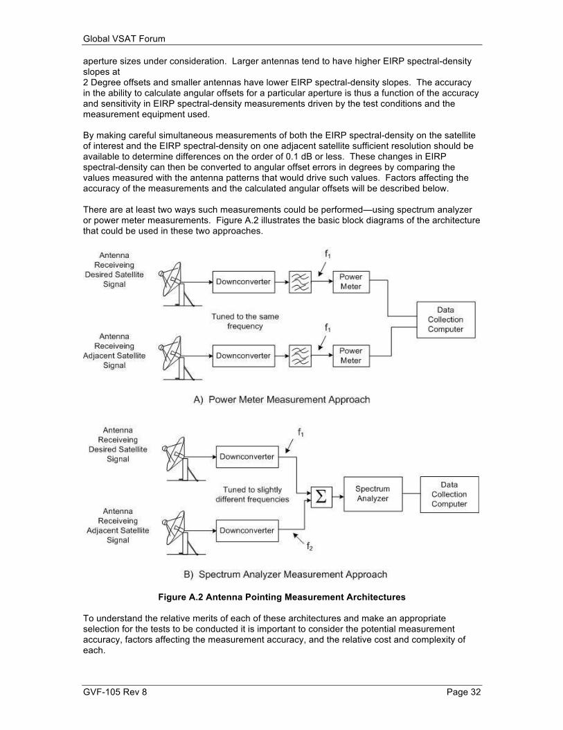
aperture sizes under consideration. Larger antennas tend to have higher EIRP spectral-density slopes at 2 Degree offsets and smaller antennas have lower EIRP spectral-density slopes. The accuracy in the ability to calculate angular offsets for a particular aperture is thus a function of the accuracy and sensitivity in EIRP spectral-density measurements driven by the test conditions and the measurement equipment used. By making careful simultaneous measurements of both the EIRP spectral-density on the satellite of interest and the EIRP spectral-density on one adjacent satellite sufficient resolution should be available to determine differences on the order of 0.1 dB or less. These changes in EIRP spectral-density can then be converted to angular offset errors in degrees by comparing the values measured with the antenna patterns that would drive such values. Factors affecting the accuracy of the measurements and the calculated angular offsets will be described below. There are at least two ways such measurements could be performed—using spectrum analyzer or power meter measurements. Figure A.2 illustrates the basic block diagrams of the architecture that could be used in these two approaches.

Figure A.2 Antenna Pointing Measurement Architectures To understand the relative merits of each of these architectures and make an appropriate selection for the tests to be conducted it is important to consider the potential measurement accuracy, factors affecting the measurement accuracy, and the relative cost and complexity of each.

Global VSAT Forum

GVF-105 Rev 8

A.1 Signal + Noise Measurements The downlink signals present at each downlink antenna will consist of the desired signal plus noise, or (C+N). The objective of the measurement in each case is to measure the signal, or Carrier power spectral-density levels, C, and not the noise. Noise is present in each of the downlink signals so accurate measurements of Carrier power spectral-density can only be made if the noise energy is sufficiently low as to be insignificant to the Carrier measurements or it must be mathematically removed. Power meters measure all the RF power, P, within their detector’s broad frequency coverage range. In general, that amounts to several GHz of potential sensitivity bandwidth. Spectrum analyzers combine a filter and detector function in one package. They make several (C+N) measurements, always reduced to power spectral-density because they use a pre-detector filter to limit the power P arriving at the detector, with each sweep. Thus, with the Power Meter method we begin with Power measurements and with the spectrum analyzer we begin with power spectral-density measurement. However, with either technique we are faced with the need to reliably measure Carrier power spectral-density while eliminating the effects of Noise power spectral-density. The downlink signals of interest can be considered to simultaneously consist of: Downlink Power = P = C+N (Equation 1) Where P = Power (observed at the measurement device) C = Carrier Power (the signal desired to be measured) N = Noise Power (which must be eliminated) Noise power present in the downlink signal can be further characterized as a specific Noise Power spectral-density in the bandwidth of interest. (In the case of a Power Meter, the bandwidth of interest is, unfortunately, the entire detector sensitivity bandwidth.) This relationship can be shown mathematically as: Noise Power = N = N0 x B (Equation 2) Where N = Noise Power (which must be subtracted for accuracy) N0 = Noise Power spectral-density B = Bandwidth (of the measurement bandwidth) The value desired for measurement is the Carrier Power, C. Since Equation 1 demonstrates that the value observed is actually Downlink Power, C+N, we must mathematically remove the contribution of Noise Power, N, to make the desired measurement. This leads to our true measurement objective being: Carrier Power = C = (C+N) - N (combining from Equation 2 produces) C = (C+N) - N0 x B (Equation 3) Where C = Carrier Power (the signal desired to be measured) (C+N) = Carrier plus Noise power (observed in measurement) N0 = Noise Power spectral-density B = Bandwidth (of the measurement bandwidth) N = Noise Power (which must be eliminated) A.2 Consideration of the Power Meter approach Power Meters are designed to make very accurate absolute RF power measurements. With the very broad bandwidth associated with Power Meter detectors it would be virtually impossible to

Global VSAT Forum

GVF-105 Rev 8

make accurate measurements of the downlink signal using a Power Meter directly. The reason for that is simply that even a very low value of N0 would be multiplied by the very broad measurement bandwidth and it would then be difficult to utilize Equation 3 above to calculate the Carrier Power C. They are not designed to make power spectral-density measurements but can make such measurements with the aid of a pre-detector filter as shown in Figure A.2 A above. As illustrated in Figure A.2 A, a filter can be inserted ahead of the Power Meter detector for the specific purpose of reducing the bandwidth B affecting the (C+N) measurement values. As bandwidth B is reduced to a very small value, and the Carrier Power C remains very narrow in frequency such as resulting from a CW signal, the contribution of C in Equation 1 above becomes much more significant than N. The complications induced in the measurements by utilizing such a filter are:

- measurement accuracy/calibration of each Power Meter detector must remain well-matched to ensure maximum accuracy.

- gain stability of the downconverter in each measurement leg can affect accuracy - absolute bandwidth accuracy of each filter must be well-matched to ensure maximum

accuracy - for very narrow filter bandwidths, the center frequency of each signal must remain reliably

within the filter passband to ensure maximum accuracy For absolute accuracy, C is determined using Equation1 and Equation 3 above. However, for the cases where C is significantly larger than N, or C >> N, then the effect of N is lower than the measurement system accuracy. One can mathematically consider the measurement impact Noise contributions would have. With the Power Meter approach, it is very difficult to generate a strong enough (C+N) signal as to make the contribution of N insignificant. A good test of such conditions is to eliminate the C energy, by turning off the transmit signal, and observing the resulting N component on its own. A value of N that is significantly below the value of (C+N) can be shown mathematically to have an impact on the value of C because the bandwidth B factor can be very wide in a Power Meter. At higher differences between C and N, the impact on determination of the value of C is less significant but must still be considered. Using a Power Meter to make the measurements without a pre-detector filter would be impossible because it would be impossible to characterize N0 across the entire measurement Bandwidth B. With a pre-detector filter one need only calibrate the N0 value within the filter bandwidth. A.3 Consideration of the Spectrum Analyzer approach Spectrum analyzers are designed to make very accurate relative power spectral-density measurements. They do not exhibit great degrees of absolute power measurement accuracy, and must be periodically calibrated to ensure the best possible accuracy in such measurements. However, spectrum analyzers have other inherent advantages. One is that they can make very rapid measurements. While Power Meters have some specific settling time, which is based on the absolute RF energy levels arriving at their detectors, spectrum analyzers are designed for rapid swept-frequency measurements. Spectrum analyzers can be considered to perform the type of measurements represented by half of Figure A.2 A above in one box. They utilize an oscillator, operating either in fixed-tuned or frequency sweeping modes, to convert frequencies entering the input to the spectrum analyzer to a fixed IF frequency which then passes through a bank of selectable filter bandwidths to a fast power detector. In the type of measurements anticipated here, spectrum analyzers contain a range of available IF filters which can closely match the characteristics of the downlink signal. A very narrow filter has the effect of significantly reducing the Noise power component N contained in the (C+N) measurement. The reason for that is that a narrow filter imposes a narrow bandwidth, B, on the (C+N) measurements and from Equation 3 above the result is less total N energy in the (C+N) measurement. Spectrum analyzers make these measurements by collecting the individual detector power spectral-density measurements on a periodic basis. Typical Agilent spectrum analyzers, for example, record 700 or 1000 individual power spectral density measurements on each sweep.

Global VSAT Forum

GVF-105 Rev 8

(An HP 8566 spectrum analyzer, for example, records 1001 measurement points in each sweep which can be as fast as 20 ms per sweep. The measurements are spaced evenly as a fraction of the spectrum analyzer frequency span in scanning measurements, or evenly as a fraction of the total time in a time-based sweep.) These individual measurements are available on the screen and for output to a recording device. Additionally, spectrum analyzers utilize measurement “markers” which can quickly report the power spectral-density measurements of specific frequencies or time offsets. On a spectrum analyzer one observes (C+N) spectral-density directly. Each one of the spectrum analyzer measurements described above actually represents the total (C+N) power contained within the spectrum analyzer Resolution Filter bandwidth at the frequency of the measurement. One could utilize two separate spectrum analyzers to independently measure the downlink signal from both the satellite of interest and the adjacent satellite. Such an approach would essentially simply replace the filters and Power Meters in Figure A.2 A with separate spectrum analyzers. However, the approach in Figure A.2 B goes one step further in simplifying the measurement configuration while actually improving measurement accuracy. The approach illustrated in Figure A.2 B takes advantage of the fact that spectrum analyzers have improved relative measurement accuracy over absolute measurement accuracy. It also takes advantage of spectrum analyzers’ inherent ability to make multiple quasi-simultaneous measurements with no degradation in measurement accuracy. Essentially, the two downlink signals in Figure A.2 B arrive at the respective terminal downlink IF outputs at essentially the same frequency. (The only factor causing any potential differences in downlink IF frequency from each terminal would be differences in the terminal Block Downconverter Local Oscillator frequencies, different satellite transponder Local Oscillators, or different Doppler effects on the two satellites. The probability of differences being significant enough to differentiate the downlink signals in a spectrum analyzer measurement is very low.) The two downconverters in Figure A.2 B are then tuned to slightly different frequencies. Such tuning can be accomplished by using slightly different 10 MHz reference input frequencies for the downconverters, as it will permit differences smaller than the typical tuning step size of synthesized downconverters. This step will permit the two signals to arrive at the spectrum analyzer at frequencies sufficiently different that the (C+N) measurement from one is not affected by the (C+N) energy from the other. To permit both signals to be measured by a single spectrum analyzer, a power combiner is utilized ahead of the spectrum analyzer input. Under such conditions, the Noise energy from the two terminals combines to potentially degrade (C+N) measurement accuracy. If the N0 energy from both terminals were exactly the same, the observed N energy would increase by 3 dB from that produced by a single terminal. If one were to be significantly less than the other, as in the (C+N) measurement discussion above, one would be dominant. However, if the sum of the two Noise power signals is still 10 dB below each of the (C+N) measurements, the impact on determining C would be low. Figure A.3 illustrates how a spectrum analyzer display of the two downlink signals, measured simultaneously, might appear. In this case, the desired signal is the lower frequency signal. It is measured on the spectrum analyzer display with a Marker on the signal peak—in this example at a frequency of 69.900 MHz and amplitude of 8.20 dBm. The second signal, from the adjacent satellite, is shown with a Delta Marker, in this case showing a Delta frequency of 200 kHz and Delta amplitude of -3.60 dBm. To make accurate measurements under such conditions, it is important that the (C+N) energy of each carrier is clearly distinct, as illustrated in Figure A.3, and do not overlap in frequency. There will already be some measurement contribution from the Noise energy of both downlinks, as described above, but if the (C+N) energy also overlaps in frequency it will be very difficult to subtract the adjacent C power to maximize measurement accuracy. Additionally, as described in previous sections the peak (C+N) power measurement should be at least 10 dB above the Noise Floor (approximately -4 dBm in this example) to ensure the effect of the Noise contribution to (C+N) is low. In the example, the Marker Delta shows approximately 8.4 dB in excess of the

Global VSAT Forum

GVF-105 Rev 8

noise floor so the measurement setup should actually be changed to ensure that both (C+N) signal peaks are 10 dB or more above the Noise Floor to provide improved accuracy.

Figure A.3 Simultaneous dual CW Signal Measurement Spectrum Analyzer Display Utilizing this technique, simultaneous measurements of the (C+N) energy contained in the downlink from the desired satellite as well as (C+N) energy contained in the downlink from the adjacent satellite can be made. The results of the measurements could be recorded by a Data Collection Computer in two ways. The first approach would be to simply record the complete trace data from each sweep of the spectrum analyzer. This would result in the accumulation of a large amount of recorded data for relatively little measurement information, since the measured (C+N) values of each carrier are all that are really required. However, it would provide a record of the spectrum actually being observed that might preclude any doubts about (C+N) above the Noise Floor and interference issues. Additionally, the time required for the spectrum analyzer to report the complete trace data to the Data Collection Computer is often significantly longer than the actual sweep time. In such cases, the test and measurement system would be limited by the spectrum analyzer / Data Collection Computer communication time rather than the actual spectrum analyzer sweep time. The alternative approach would be to record simply the Marker and Delta Marker information from the spectrum analyzer. This is a much smaller data set for each measurement point and is thus much faster to communicate from the spectrum analyzer to the Data Collection Computer. It would thus be limited simply by the spectrum analyzer sweep time and not by the spectrum analyzer / Data Collection Computer communication time. The only drawbacks to this approach

Global VSAT Forum

GVF-105 Rev 8

are that there would be no absolute record that each measurement resulted in (C+N) values sufficiently above the Noise Floor to ensure maximum accuracy, and there would be no record that interference did not affect the measurements. Still, an operator conducting the measurements could ensure through observations prior to the commencement of data collection that these two desired conditions are met. The spectrum analyzer will continue to display the full sweep data visually during the test process, so ongoing visual observation could confirm that the desired measurement conditions were met. An additional measurement simplicity is also offered by this measurement approach. If the spectrum analyzer is set to “Max Hold” during the measurement period, it will record the highest signal level for each “bin” in the continuous spectrum analyzer sweeps during the measurements. Thus, the highest values observed by the spectrum analyzer for the (C+N) of the satellite of interest downlink signal as well as the (C+N) of the adjacent satellite downlink signal will be recorded. This would give an absolute maximum tracking error signal indication because it would record the highest level observed in the downlink of the adjacent satellite. For measurements in which it is desired to ensure that antenna pointing and tracking are within some preset limit, this would provide absolute assurance of such conditions without even the need for a Data Collection Computer. For conditions of considerable variation in either or both of the downlink signals, this measurement may be of little value. However, for the normal VMES operating case where antenna tracking is expected to be extremely accurate, it can provide a quick “Go / No-Go” confirmation of satisfying tracking performance objectives. A.4 How to make accurate CW signal measurements using a Spectrum Analyzer Since a spectrum analyzer will be used to make the downlink (C+N) measurements, it is imperative that the tests be conducted by an operator who knows how to make accurate spectrum analyzer measurements under these conditions. Specifically:

- The downlink signals will consist of essentially CW tones. - Peak (C+N) values will be 10 dB or more above the Noise Floor of the measurement

setup.

- Peak (C+N) values will be far enough in frequency that the presence of C energy from one carrier will have negligible impact on the C energy measured from the adjacent carrier.

- The spectrum analyzer will perform swept frequency measurements at sweep speeds

consistent with the spectrum analyzer maximum measurement accuracy. Spectrum analyzers make power spectral-density measurements by tuning an oscillator such that a precise IF filter can be used to select the bandwidth of power spectral-density that is measured by the spectrum analyzer detector. In conducting this operation, there are several significant factors which affect measurement accuracy. The IF filter used by the spectrum analyzer to select the increment of RF spectrum reaching the detector is called the “Resolution Bandwidth” filter. It must be very precisely measured and controlled to ensure spectrum analyzer measurement accuracy and repeatability. Spectrum analyzers typically have internal calibration routines which use a CW tone input to the spectrum analyzer which then adjusts the shaping and amplitude of the raw measurement data based upon the designed Resolution Bandwidth characteristics. After the spectrum analyzer has run its internal calibration routine, it should be able to make very accurate power spectral-density measurements that are repeatable from one Resolution Bandwidth to another. Agilent spectrum analyzers typically contain a range of Resolution Bandwidth filters in 1,3, 10 bandwidth increments. For example, a particular Agilent spectrum analyzer might have Resolution Bandwidths of 10 Hz, 30 Hz, 100 Hz, 300 Hz, 1 kHz, 3 kHz, 10 kHz, 30 kHz, 100 kHz, 300 kHz, and 1 MHz available. The bandwidth selected for CW measurements is critical because the highest sensitivity of (C+N) measurements above the Noise Floor occur when the narrowest

Global VSAT Forum

GVF-105 Rev 8

possible Resolution Bandwidth filter is employed. Even though CW signals are essentially 0 Hz wide, the spectrum analyzer may not be able to use its smallest Resolution Bandwidth filter to make the desired measurement due to drift in the frequencies of conversion oscillators anywhere in the system of interest, or in the spectrum analyzer itself. Additionally, a very narrow Resolution Bandwidth filter takes longer for the detector to make a measurement than a wider filter, unless Digital Signal Processing (using Fast-Fourier Transforms, or FFTs) are employed. For those two reasons it is usually prudent to select a Resolution Bandwidth filter as small as possible while still providing reasonable sweep times and tolerance for combined frequency inaccuracies. After the spectrum analyzer detector, there is another filter which provides “smoothing” of the measurement result. In Agilent spectrum analyzers it is called the “Video Bandwidth” filter. A narrow Video Bandwidth filter tends to smooth out the random nature of noise effects on signal measurements. It has the effect of essentially “averaging” the detector output for a small time period following each measurement across the sweep. Wide Video Bandwidth filters permit the spectrum analyzer to observe very rapid signal fluctuations, such as modulation, which can affect the measurement data. Smaller Video Bandwidth filters require more time for the spectrum analyzer to pause and smooth the results after each detector measurement so they will slow the spectrum analyzer sweep speed. When measuring CW tones in the presence of a Noise Floor significantly below the (C+N) energy levels, it is best to select a Video Bandwidth that permits faster sweep times while still providing a noticeably “smooth” Noise Floor. If the Video Bandwidth filter is selected at too broad a bandwidth, the apparent Noise Floor might have fluctuations of several dB and thus impose random variations in the resultant C measurements when N is subtracted from (C+N). Another factor in Agilent and other spectrum analyzers is Video Averaging. That technique is quite similar in results to narrowing the Video Bandwidth, but it is achieved by averaging multiple sets of spectrum analyzer sweep data, point by point. For example, if Video Averaging is set to 4, 4 separate spectrum sweeps are performed and the data at each point in the spectrum analyzer display is averaged for the measurements at that exact frequency point in each of the 4 sweeps. As additional sweeps are performed, the spectrum analyzer continues to display a “running average” calculated by averaging the prescribed number of previous sweeps. Video averaging can effectively flatten the Noise Floor and permit reliable measurements of Noise energy in a way which is faster than using a narrow Video Bandwidth, and that is the main reason it was developed. For the purposes of our measurements here, we should be able to make reasonably fast measurements using a suitably small Video Bandwidth filter rather than resorting to Video Averaging which could degrade the absolute (C+N) measurements. Finally, spectrum analyzers typically conservatively calculate the sweep time requirement to make a particular measurement based on the operator-selected values of Resolution Bandwidth and Video Bandwidth. It does that by calculating the time required for the spectrum analyzer detector to accurately respond to the input signal power spectral-density given the established filter settings. In most spectrum analyzers this internal calculation can be “over-ridden” by direct operator input of Sweep Time. There are some cases in which this might make sense, such as when observing the signal modulation characteristics rather than making accurate power spectral-density measurements. However, CW measurements as described here are not such a case. For the maximum CW measurement accuracy, the spectrum analyzer’s internally-calculated Sweep Time should be used, and not forced by operator intervention. Most spectrum analyzers will report a special “Uncalibrated” message when a Sweep Time below that calculated by the spectrum analyzer is selected. It is important for best measurement accuracy here that such messages are not generated during operation. Figure A.4 illustrates a spectrum analyzer display for a representative CW signal measurement. In this example, the signal of interest is centered at 70 MHz and Marker 1 displays its measurement frequency of 70.000 MHz and amplitude of 8.01 dBm. It should be recalled for the earlier discussion that the value of 8.01 dBm actually represents the (C+N) valued observed by the spectrum analyzer, and not the value of C itself.

Global VSAT Forum

GVF-105 Rev 8

Figure A.4 Single CW Signal Measurement Spectrum Analyzer Display To be able to make an accurate measurement of C, it is necessary to have a reference of the N value contained in the (C+N) value so it can be mathematically subtracted. In the example of Figure A.4 this Noise measurement is made with Marker 2 and shown at frequency 70.08 MHz and amplitude -4.00 dBm. One of the considerations when making such measurements is where to make the Noise measurement. The value of N needed is that exactly at the frequency of the (C+N) measurement. Since we can’t perform the measurement at that exact frequency, we select one as close as possible which will represent the apparent Noise value. In the case of Figure A.4 the Noise Floor is relatively flat so an N measurement could be made almost anywhere in the spectrum analyzer trace outside the (C+N) represented by the carrier. In cases where the Noise Floor has an apparent slope, the most accurate N measurements are actually made by assuming the Noise Floor to be smooth in the dB domain, and making measurements on each side of the carrier of interest and then averaging the two. Having collected the measurement data represented by Figure A.4 one could then calculate the amplitude of the Carrier Power, C. To do so, we utilize Equation 3 above, which is: C = (C+N) - N0 x B (Equation 3) The essential steps in calculating accurate values of C from the spectrum analyzer observations are to:

Global VSAT Forum

GVF-105 Rev 8

1) Convert (C+N) values to linear power units 2) Calculate N by multiplying N0 over the Resolution Bandwidth B, or use the N value

from the spectrum analyzer directly 3) Convert N into linear power units 4) Subtract N from (C+N) to determine C, in linear power units 5) Convert C from linear power units to dBm or dBW

These steps will be performed below using the measurements in Figure A.4 as an example. Marker 1 represents (C+N), but in log units of dBm. Converting (C+N) from log (dBm) units to linear power units we determine that: 8.01 dBm = 6.324 milliwatts = (C+N) Spectrum analyzers can measure the Noise Floor by setting a marker, as shown in Figure A.4, or the “Marker Noise” function can be selected on the spectrum analyzer in which case it will calculate N0 directly from the measurement. In the example of Figure A.4 we conclude that the marker 2 measurement is the total N power contained in one Resolution Bandwidth of the spectrum analyzer. Thus, it can be used directly and we must simply convert it to linear power units. We calculate that: -4.00 dBm = 0.3981 milliwatts = N Now, we calculate C by subtracting N from (C+N) as described in Equation 3. C = 6.324 milliwatts – 0.3981 milliwatts = 5.926 milliwatts Converting to dBm: C = 5.926 milliwatts = 7.728 dBm It would be this value, C, that would be utilized in the antenna pointing measurements to compare the changes in downlink power that would be expected for a given antenna pointing error. A.6 Factors which might affect signal measurement accuracy Several different factors should be considered which might affect the accuracy of the measurements obtained. Some of these are a function of the test equipment setup and can be controlled while establishing test conditions and others are environmental which should be monitored during the period of the test. The description below will consider these potential factors and propose methods to constrain their affects.

1) Propagation impacts. Obviously, VMES operations are susceptible to all the same propagation effects as all FSS Ku-Band signals. Additionally, the VMES environment produces a large number of signal blockage conditions when antenna look angles are obstructed by buildings, utility poles, vegetation, and other objects. Careful VMES testing should only be performed under reasonably “clear sky” conditions to ensure rain fades or other similar propagation degradations are not encountered. Signal blockage cannot reasonably be avoided in VMES operation, so about the only mitigation for these effects is to attempt to utilize conditions which would block the signal path to the target satellite and adjacent satellite used for the test in the same way. This can likely be best confirmed if suspicious results appear in the measurement data. For example, in most VMES blockage conditions a vehicle would pass from “clear” to “blocked” conditions in a way that would result in downlink levels on the target and adjacent satellite about equally. If the test data suggests this not to be the case, consideration should be given to the exact blockage conditions which might produce such results.

Global VSAT Forum

GVF-105 Rev 8

2) Vehicle dynamics. VMES terminals are designed to satisfy operational requirements under a specific set of dynamic conditions. While these conditions are not specified by the FCC, they are often specified in customer requirements documents or specifications. Such levels of vehicle dynamics are actually one of the differences in the design of different VMES systems and can serve as market differentiators. VMES testing can be performed using carefully instrumented vehicle dynamics or it can be performed using available test vehicles, road surfaces, or “test track conditions”. For repeatability, VMES testing should be performed in some controlled way such that the vehicle dynamics are either carefully measured or repeatable. Excessively high dynamics should be expected to have the result of degrading VMES antenna pointing test data.

3) Satellite transponder linearity. Measuring antenna offset angles in the approach

described here presumes that the transponders on both the desired and adjacent satellites are operating in a linear mode. Thus, efforts should be made to ensure that signal levels on both satellites are significantly below saturation and well within the linear region. Additionally, efforts should be made to confirm that during the period of the test there are no unusual satellite transponder operations like gain state changes, transponder signal level fluctuations that might be caused by high-level TDMA signals, etc. Linear operation can be confirmed by observing transponder power prior to beginning the test. Transponder gain stability can be confirmed by a period of signal monitoring prior to beginning the test.

4) Test system linearity and stability. Just as transponder linearity can affect the test

data, the test setup itself can also affect measurement accuracy. All amplifiers and frequency converters used in the test setup must be confirmed to be operating in their linear range and without any variations in gain or frequency. For maximum accuracy the test setup should be in operation for a considerable period of time before actually beginning the tests to ensure that all associated equipment has stabilized in temperature and frequency prior to making any measurements. Frequency sources in every converter should be confirmed to be phase-locked and stable. Gain of all amplifiers and frequency converters in the test setup should be confirmed stable and free from any significant fluctuation in temperature, primary power, or other factors. It should be confirmed by monitoring that during the entire test period the frequency of the downlink signals both on the desired and adjacent satellites have not drifted enough to degrade spectrum analyzer measurements. (This would likely be most significant if the spectrum analyzer were to be used in a fixed Marker mode. In such cases the spectrum analyzer marker stays on exactly the frequency set at the start of measurements. Frequency drift farther than a single Resolution Bandwidth filter bin in the spectrum analyzer would then cause the Marker to produce faulty measurements.) Obviously, no changes in any element of the test setup should be made while measurements are actually being collected.

5) Test signal levels sufficiently above the Noise Floor. Since the test measurements

require accurate determination of C power above the satellite transponder and test equipment Noise Floor, steps should be taken to ensure RF and IF power levels are sufficient for measurement. This should be confirmed through multiple verifications prior to conducting the test. Specifically:

a. To ensure the spectrum analyzer noise floor is not affecting measurements,

after the test setup is configured, including the specific spectrum analyzer frequency, amplitude, sweep, and filter settings, the input from the spectrum analyzer can be temporarily disconnected. The Noise Floor on the spectrum analyzer in the absence of any input signal should be confirmed to be more than 10 dB below the Noise Floor for the test signals themselves.

b. The G/T of the downlink test terminals can degrade measurement accuracy if

it is not high enough to make reliable Noise measurements. If the two

Global VSAT Forum

GVF-105 Rev 8

downlink test terminals have differing G/T performance, the terminal with the better G/T should be utilized on the adjacent satellite rather than the desired satellite because the adjacent satellite will operate at lower absolute signal levels. Each downlink signal should be temporarily removed from the power combiner ahead of the spectrum analyzer and expected changes in measured Noise Floor confirmed. (If the G/T of the downlink test terminals, removing either input should cause a 3 dB decrease in measured Noise Floor. If one is significantly better than the other, removal of the signal from the terminal having the higher G/T should have relatively little impact on the measured Noise Floor.)

6) Inaccuracies in antenna patterns. The test technique utilized here presumes that the

VMES transmit antenna radiation patterns are performing as previously measured. There are several factors which might cause the measurements to diverge from the previous antenna pattern measurement conditions. These include such factors as:

a. Antenna patterns are measured in the azimuth and elevation planes. The

desired and adjacent satellites will rarely be in exactly only the azimuth plane. Circular VMES antennas will have radiation patterns that are similar in all planes. Non-circular VMES antennas will have radiation patterns that could exhibit differences in planes that further pattern estimation may well be required.

b. Radomes mounted on the VMES antennas will have some impact on the

antenna radiation patterns. As a first approximation, the tests describe here will disregard the radome effects. Depending upon the results obtained, it may be prudent to run a series tests with the radome installed and another with the radome removed to quantify the potential impact on radiation patterns.

Global VSAT Forum

GVF-105 Rev 8

Appendix B: The Faciltiy for Over-the-air Research and Testing FORTE at Fraunhofer IIS As an Authorized Test Entity ATE of the GVF, the Facility for Over-the-air Research and Testing FORTE offers an environment for testing SOTM terminals under realistic conditions. FORTE was built by Fraunhofer IIS in collaboration with the Teschniche Univeraität in Ilmenau. FORTE offers emulation of the complete SOTM reality on earth without the involvement of operational satellites or real motion platforms (vehicles). Hardware in Ku- and Ka- frequency bands mounted on a 50 meters antenna tower is used to emulate the operational GSO satellite. The terminal under test is fixed on a 3-axis motion emulator which can replay the movement introduced by the vehicle. A channel emulator reproduces both the fading caused by obstructions to the Line-of-Sight (LoS) and the one caused by adverse weather conditions. Moreover, a GPS emulator is available to be used for terminals which need GPS lock. A block diagram with the full structure of FORTE is shown in Figure B.1.

channelemulator

channelemulator

+

motionemulator

anechoicchamber

SatComterminal(deviceundertest)

GPSemulator

laboratorybuilding

antennatower

synchronizedprofileplayback

IF=140MHzL-Bandcontrol

downlink:12/20GHz

uplink:14/30GHz

Ku/Ka-Band

wiredconnection(optional)

depointingmeasurement

cross

TestbedSatCom

networknetwork

datastream

SatComterminals

satelliteemulator

network

Testfacility»AmVogelherd«inIlmenau Figure B.1 Components of FORTE

The distance between the terminal and the antenna tower is about 100 m. This distance allows for far-field tests for most high gain antennas (e.g. dishes with up to 90 cm diameter in Ku-Band, or 70 cm in Ka-Band). The structure at FORTE enables also for XPD measurements in far-field. In order to test and validate the antenna pointing accuracy, a cross shaped sensor array with six antennas is mounted on the antenna tower. The detailed process of the antenna de-pointing measurements is described in section B.1. FORTE compared to the traditional testing approaches which use operational satellites, yields the following advantages:

•a higher accuracy in evaluating the pointing errors •independence of the weather and of the satellite availability •allows for repeatability, while choosing any arbitrary parameter set (motion profile, fading profiles, etc.).

B.1 Antenna De-pointing Measurements

Global VSAT Forum

GVF-105 Rev 8

De-pointing estimation at FORTE is done using a cross shaped sensor array as shown in Figure B.2. The distance d between the sensors on the tower can be changed w.r.t. the 3dB beam width of the antenna under test in order to improve the estimation accuracy. Based on simulations, an empirical formula for the optimum positions of the sensors w.r.t. the SNR and the 3 dB beam width of the antenna (ω) is derived:

Δ = [a•ρ3+b•ρ2+c•ρ +d] •ω --(EquationB.1) Where

• Δis the distance of the outer sensor to the centered sensor along horizontal as well as vertical axes (cf. Figure B.2)

• ρ is the SNR in dB • ωis the 3 dB beam-width of the antenna in degrees • with the polynomial coefficients a=−1.3•10-6, b=1.8•10-4, c=−7.2•10-3and d=0.709

Figure B.2 De-pointing Measurements at FORTE

The maximum achievable estimation accuracy (expressed in terms of standard deviation of the estimated antenna de-pointing) corresponding to the optimum sensor positions is plotted in Figure B.3. From Figure B.3, if we fix the beam width (ω) and look along a horizontal line it can be seen that the higher the available SNR, the better the estimation accuracy can be. If we fix the SNR (ρ) and look along a vertical line, it can be seen that the wider the beam width, the worse the estimation accuracy will be.

Global VSAT Forum

GVF-105 Rev 8

Figure B.3 Estimation accuracy (expressed in terms of standard deviation of the

estimated antenna de-pointing) for the optimum sensor positions Δ w.r.t. the 3 dB antenna beam width ω and SNR in dB ρ.

However, in practice the adjustment of the sensors can be very time consuming. If one wanted to test subsequently various terminals with different antenna beam widths, it would be preferable to keep the sensors at fixed positions for all tests. By defining a minimum de-pointing estimation accuracy (e.g., 0.05deg) that has to be achieved in any case, a region w.r.t. sensor position and antenna beam width can be defined achieving at least the minimum accuracy at a certain SNR. According to Figure B.4, the sensor position can be chosen in a wider range.

Figure B.4 Minimum SNR regions for which an estimation accuracy better than

0.05deg can be achieved. For a higher SNR a larger region is obtained.

Global VSAT Forum

GVF-105 Rev 8

In a preliminary measurement for the determination of antenna de-pointing, the received power at the six sensors is measured for different known antenna de-pointing directions while the tracking mechanism of the SOTM terminal is disabled. This data serves as reference for the de-pointing estimation, in which the motion emulator replays a certain motion profile while the tracking system is active. At this point, the estimation is carried out in three steps (cf. Figure B.2):

1) measure the received signal from the antenna at the six sensors 2) calculate the correlation between the measured signal and the reference data 3) the antenna de-pointing estimate results from the maximum of the correlation.

B.2 Image Based Land mobile Satellite LMS Channels The channel emulators at FORTE can emulate realistic fading profiles. An image-based approach to determine the Land Mobile to Satellite (LMS) channel was developed at Fraunhofer IIS [6]. The channel fading is characterized by a statistical based approach to distinguish between good (Line Of Sight LOS) and bad (Light shadowing and Non-LOS) states. A hemispheric image of the environment is obtained from a fisheye camera pointing towards the sky. Such an image is depicted in Figure B.5(a). A categorization algorithm divides the hemispheric image into the region sky, where a satellite would be visible and the region obstruction, where it would be shadowed by an object. An example of this categorization is given in Figure B.5(b), where sky is depicted in blue and obstruction in red.

(a) An exemplary hemispheric image (b) An overlay consisting of the original and the binary categorization into sky and obstruction

Figure B.5 The images show the original hemispheric image and the result of

the image categorization.

In a second step, the conversion from the processed fisheye images to rectangular binary image in landscape panoramic form is performed, as shown in Figure B.6. The reception state can be extracted directly from this image, where white represents good and black bad state, respectively. By simple geometric considerations, knowing the time and location information of the vehicle, we can extract the reception states for any possible satellite position using the panoramic images.

Figure B.6 The converted panoramic binary images are of size 90×360 pixels, where the

resolution is one degree in elevation and in azimuth. White represents the receptions state good and black bad, respectively.

The channel emulator at FORTE is based on the sequence of reception states derived from images. An extensive validation of the method can be found in [6], where we consider simultaneously recorded Radio

Global VSAT Forum

GVF-105 Rev 8

Frequency (RF) signal levels as a reference. The results of the verification demonstrate that the image-based approach is a reliable method for availability prediction for arbitrary satellite positions. Figure B.7 shows an exemplary fading sequence which can be emulated at FORTE. The sequence is for a satellite at 25° in elevation and 10° in azimuth for two different environment types: suburban and highway. Weather conditions can be also added to the emulation process e.g. rain fades where the whole time sequence will be shifted down by the rain fade factor as shown in Figure B.8.

Figure B.7 Examples of fading profiles as power levels over time for different environments suburban and highway for a satellite positioned at 25° elevation and 10°

azimuth.

Figure B.8 Exemplary fading profiles as power levels over time in urban environment for a

satellite positioned at 25° elevation and 10° azimuth. The received satellite signal characteristic for sunny weather is plotted in violet and for rainy weather in red,

respectively. The vertical axis represents the signal level in dB where 0 dB corresponds to LOS

B.3 Performance Measurements at FORTE The motion profiles for Class A and Class B have been applied at FORTE on real SOTM terminals from key market actors. The results from one terminal are presented in this section.

B.3.1 Antenna measurements: The terminal has a 65 cm dish antenna operating in Ka-band. The transmit (Tx) and receive (Rx) patterns are measured as a first step. The transmit frequency is 30.095 GHz and the receive frequency is 20.295 GHz. Figures B.9, B.10 and B.11 show the Tx, Tx_XPol and Rx patterns of the antenna at the defined frequencies.

Global VSAT Forum

GVF-105 Rev 8

Figure B.9: Tx absolute gain pattern of the SOTM antenna under test

Figure B.10: Tx_XPol pattern of the SOTM antenna under test

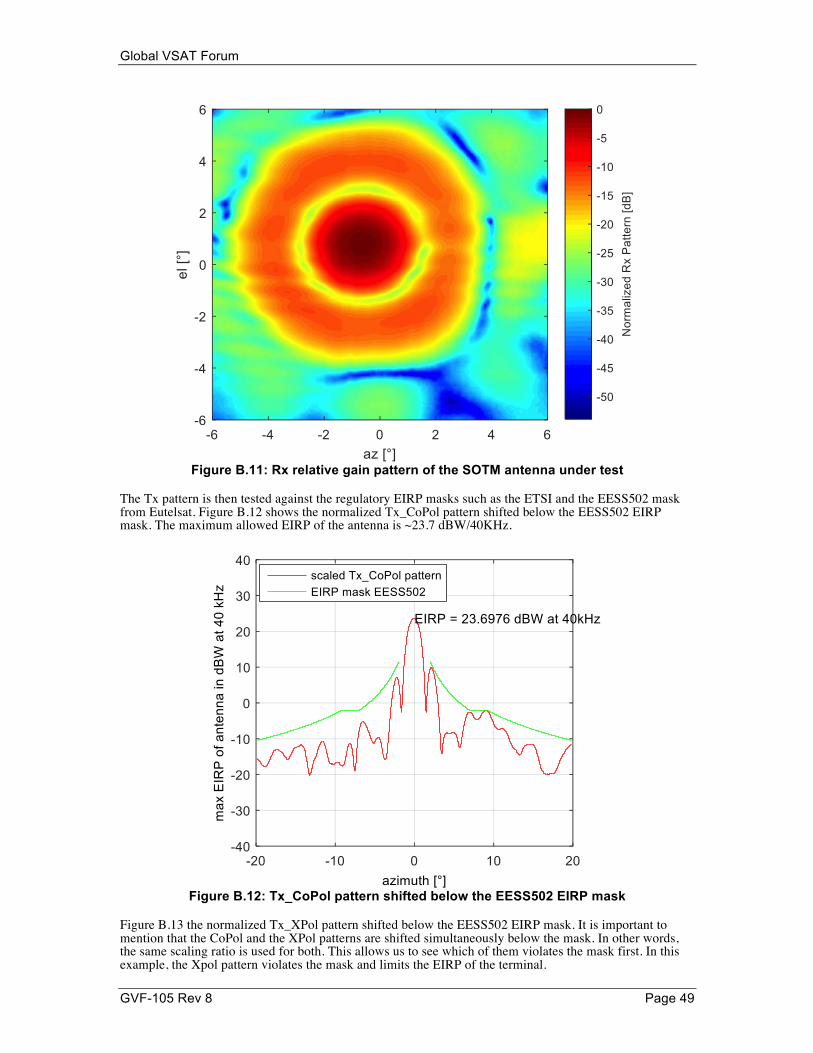
Global VSAT Forum

GVF-105 Rev 8

Figure B.11: Rx relative gain pattern of the SOTM antenna under test

The Tx pattern is then tested against the regulatory EIRP masks such as the ETSI and the EESS502 mask from Eutelsat. Figure B.12 shows the normalized Tx_CoPol pattern shifted below the EESS502 EIRP mask. The maximum allowed EIRP of the antenna is ~23.7 dBW/40KHz.

Figure B.12: Tx_CoPol pattern shifted below the EESS502 EIRP mask

Figure B.13 the normalized Tx_XPol pattern shifted below the EESS502 EIRP mask. It is important to mention that the CoPol and the XPol patterns are shifted simultaneously below the mask. In other words, the same scaling ratio is used for both. This allows us to see which of them violates the mask first. In this example, the Xpol pattern violates the mask and limits the EIRP of the terminal.

Global VSAT Forum

GVF-105 Rev 8

Figure B.13: Tx_XPol pattern shifted below the EESS502 EIRP mask

B.3.2 Tracking Performance: FORTE has an accurate de-pointing estimation system for SOTM terminal [6]. A sensor array is mounted on an antenna tower and a motion emulator is holding the SOTM terminal in an anechoic chamber 100 m away. This setup enables full system test in a controlled environment for the SOTM terminals. The tracking performance of the antenna is evaluated by measuring the de-pointing of the antenna while being in motion. The motion profile of the Class A and Class B have been applied to the terminal under test.

B.3.2.1 Performance under Class A profile:

Figure B.14 shows the performance of the antenna under Class A motion profile. The de-pointing is estimated for the azimuth and elevation axes. The CDF of the estimated de-pointing is plotted in Figure B.15. Figure B.14 shows that the antenna has a constant de-pointing offset (~ -0.2°) in elevation due to manufacturing. For most of the satellite operators, the antenna de-pointing in elevation is not of interest.

Global VSAT Forum

GVF-105 Rev 8

Figure B.14: De-pointing estimation of the terminal under test for azimuth and elevation

under Class A motion profile

Figure B.15: CDF of the de-pointing estimation of the terminal under test for azimuth and

elevation under Class A motion profile

Global VSAT Forum

GVF-105 Rev 8

B.3.2.2 Performance under Class B profile: Figure B.16 shows the performance of the antenna under Class B motion profile.


under Class B motion profile The CDF of the estimated de-pointing is plotted in Figure B.17.

. Figure B.17: CDF of the de-pointing estimation of the terminal under test for azimuth and

elevation under Class B motion profile

Global VSAT Forum

GVF-105 Rev 8

B.3.2.3 Performance under ChurchvilleB profile: The performance of the terminal has also been tested under the well-known ChurchvilleB motion track. Figure B.18 shows the corresponding de-pointing estimation results. Figure B.19 shows the CDFs of the estimation results.


under the ChurchvilleB motion profile

Figure B.19: CDF of the de-pointing estimation of the terminal under test for azimuth and

elevation under the ChurchvilleB motion profile

B.3.2.3 Performance under sinusoidal profile:

Global VSAT Forum

GVF-105 Rev 8

It is often desirable to test the maximum angular rate the terminal can achieve before the tracking unit starts to face troubles. A sinusoidal motion profile is synthesized and replayed at FORTE for this purpose. Figure B.20 shows the yaw stimulation profile of a sinusoidal track with amplitude of 10° and frequency of 0.75 Hz. In this example, the profile is stimulated at all axes, yaw, pitch and roll, simultaneously. Figure B.21 shows the de-pointing estimation results.

Figure B.20: The yaw stimulations of the sinusoidal motion profile

Figure B.21: De-pointing estimation of the terminal under test for azimuth and elevation under the sinusoidal motion profile with amplitude 10° and frequency 0.75 Hz at all axes

The de-pointing estimation is not shown in the interval beyond 30 seconds because the antenna was totally de-pointed. Figure B.22 shows the de-pointing estimation results versus the angular rate vector norm of the motion profile. It can be seen that above 35 °/s the tracking unit starts to face problems.

Global VSAT Forum

GVF-105 Rev 8

Figure B.22: De-pointing estimation plotted versus angular rate under the sinusoidal motion profile with amplitude 10° and frequency 0.75 Hz at all axes

For the sake of comparison, the results as well as the CDFs of the azimuth estimation for the different tracks are plotted together as shown in Figures B.23 and B.24, respectively.

Figure B.23: Azimuth de-pointing for the different motion tracks

Global VSAT Forum

GVF-105 Rev 8

Figure B.24: CDFs of azimuth de-pointing for the different motion tracks

Figure B.24 shows that the azimuth de-pointing stays below 0.2° for more than 99% of the time for all motion tracks.

Global VSAT Forum

GVF-105 Rev 8

Appendix C: Additional Notes on Standard Motion Profiles The definition of the standard motion classes in Section 5.3.5.1 (Land mobile motion profile definition) and Section 5.3.5.2 (Maritime motion profile definition) is based on an extensive measurement campaign that was performed by Fraunhofer IIS under the ESA Contract: 4000103870/11/NL/NR (under the ESA ARTES 5.1). The campaign covered various environments, terrain types and platforms. Motion dynamics were measured using a sophisticated IMU (ADMA from GENSYS http://www.genesys-adma.de/downloads.php?ID=6935&IDADMA=f9001afefe8ecc0a5543ac9a87e6cb36&IDADMA=f9001afefe8ecc0a5543ac9a87e6cb36). The motion dynamics are defined by the angular and translational behavior. Positions, rates and accelerations are the parameters which are commonly used in this sense. C.1 Data Analysis: Statistical analysis can be used efficiently to show the behavior of motion parameters. More specifically, the statistical percentiles are of interest. For example, the 95.45% percentile (Q95) indicates the value below which 95.45% of the analyzed parameter fall. The Cumulative Distribution Function (CDF) is often used to show the percentiles as in Figure C.1.

0 5 10 150

10

20

30

40

50

60

70

80

90

100

110

Parameter e.g. Angular Rate [°/s]

CDF

[%]

Q68 Q95 Q99

Figure C.1 statistical percentiles shown using the CDF

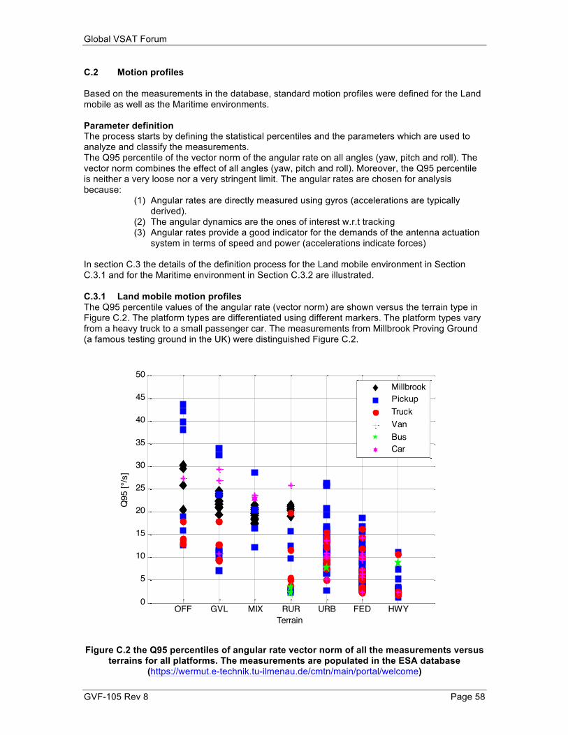
Global VSAT Forum

GVF-105 Rev 8

C.2 Motion profiles Based on the measurements in the database, standard motion profiles were defined for the Land mobile as well as the Maritime environments. Parameter definition The process starts by defining the statistical percentiles and the parameters which are used to analyze and classify the measurements. The Q95 percentile of the vector norm of the angular rate on all angles (yaw, pitch and roll). The vector norm combines the effect of all angles (yaw, pitch and roll). Moreover, the Q95 percentile is neither a very loose nor a very stringent limit. The angular rates are chosen for analysis because:

(1) Angular rates are directly measured using gyros (accelerations are typically derived).

(2) The angular dynamics are the ones of interest w.r.t tracking (3) Angular rates provide a good indicator for the demands of the antenna actuation

system in terms of speed and power (accelerations indicate forces) In section C.3 the details of the definition process for the Land mobile environment in Section C.3.1 and for the Maritime environment in Section C.3.2 are illustrated. C.3.1 Land mobile motion profiles The Q95 percentile values of the angular rate (vector norm) are shown versus the terrain type in Figure C.2. The platform types are differentiated using different markers. The platform types vary from a heavy truck to a small passenger car. The measurements from Millbrook Proving Ground (a famous testing ground in the UK) were distinguished Figure C.2.

OFF GVL MIX RUR URB FED HWY0

5

10

15

20

25

30

35

40

45

50

Terrain

Q95

[°/s

]

MillbrookPickupTruckVanBusCar

Figure C.2 the Q95 percentiles of angular rate vector norm of all the measurements versus

terrains for all platforms. The measurements are populated in the ESA database (https://wermut.e-technik.tu-ilmenau.de/cmtn/main/portal/welcome)

Global VSAT Forum

GVF-105 Rev 8

C.3.1.1 Class definition Sorting all Q95 percentile angular rate values in a descending order –as in Figure C.2–, a (Quasi-) turning point can be found. At this turning point, a separation threshold can be set. Above the threshold, the curve has a relatively high slope, while below the threshold the slope starts to decrease.

0 20 40 60 80 100 120 140 160 180 2000

5

10

15

20

25

30

35

40

45

X: 24Y: 22.24

Measuements count

Q95

[°/s

]

Figure C.3 the Q95 percentiles of angular rate vector norm of all the measurements sorted

in a descending order

Two classes can be defined based on this threshold value as shown in Figure C.4. Class A with all the measurements having Q95 percentile values above the threshold (harsh terrains as Off-road) and Class B with all the measurements having Q95 percentile values below the threshold (Paved terrains and relaxed Off-roads). The centroid and the confidence interval (standard deviation) for each class are shown in Figure C.5.

Global VSAT Forum

GVF-105 Rev 8


5

10

15

20

25

30

35

40

45

50

Terrain

Q95

[°/s

]


Figure C.4 the two classes based on the threshold value defined in Figure C.3

classA classB0

5

10

15

20

25

30

35

40

45

50

Q95

[°/s

]

Figure C.5 the centroid and confidence interval for the two classes

ClassA

ClassB

centroid

Global VSAT Forum

GVF-105 Rev 8

C.3.1.2 Profile Selection The measurement with the closest Q95 percentile value is selected as the standard representative of each class as shown in Figure C.6.


10

20

30

40

50

Terrain

Q95

[°/s

]


0

10

20

30

40

50

classA

classB

Figure C.6 the selection of the standard motion profiles based on angular rate vector norm

C.3.1.2.1 Class A standard Profile From Figure C.6 it can be seen that an off-road sinusoidal test track at the Millbrook Proving Ground has the closest angular rate norm to the Class A centroid. The effect of the individual axes on the overall dynamics of the track is then inspected. Figure C.7 shows the CDFs of the angular rates for the overall vector norm as well as the individual axes.

0 5 10 15 20 25 30 350

20

40

60

80

100

Angular Rate [°/s]

CDF

[%]

Allyawpitchroll

Figure C.7 the CDFs of the angular rates (vector norm and individual axes) for the

sinusoidal off-road track

ClassA

ClassB

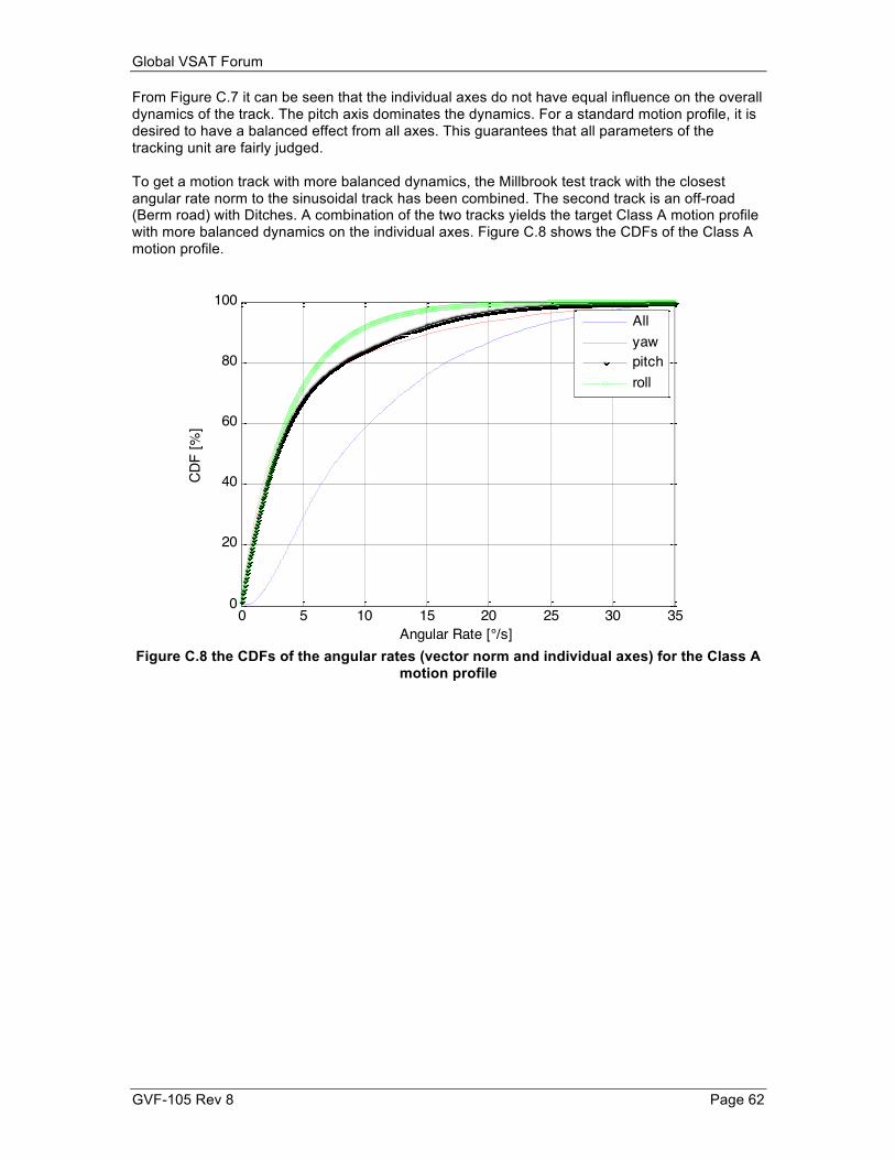
Global VSAT Forum

GVF-105 Rev 8

From Figure C.7 it can be seen that the individual axes do not have equal influence on the overall dynamics of the track. The pitch axis dominates the dynamics. For a standard motion profile, it is desired to have a balanced effect from all axes. This guarantees that all parameters of the tracking unit are fairly judged. To get a motion track with more balanced dynamics, the Millbrook test track with the closest angular rate norm to the sinusoidal track has been combined. The second track is an off-road (Berm road) with Ditches. A combination of the two tracks yields the target Class A motion profile with more balanced dynamics on the individual axes. Figure C.8 shows the CDFs of the Class A motion profile.

0 5 10 15 20 25 30 350

20

40

60

80

100

X: 27.76Y: 95.47

Angular Rate [°/s]

CDF

[%]

Allyawpitchroll

Figure C.8 the CDFs of the angular rates (vector norm and individual axes) for the Class A

motion profile

Global VSAT Forum

GVF-105 Rev 8

Figures C.9, C.10 and C.11 show the GPS data, satellite view and a location view of the Class A profile, respectively.

52.03552.036

52.03752.038

52.03952.04

52.04152.042

-0.545

-0.54

-0.535

-0.5360

80

100

120

longitude [°]

latitude [°]

heig

ht [m

]

Figure C.9 Class A profile -GPS profile-

Figure C.10 Class A profile –satellite view–

Global VSAT Forum

GVF-105 Rev 8

Figure C.11.a part1 “Sinusoidal off-road”

Figure C.11.b part2 “Berm-road with Ditches”

Figure C.11 Class A profile–platform and location view–

Global VSAT Forum

GVF-105 Rev 8

C.3.1.2.2 Class B standard Profile The same process which leaded to a classA motion profile which has balanced dynamics on all axes has been repeated for classB. The best-fit profile for Class B is a repetition of a gravel track twice. It defines a Van on a gravel/dirt road. Figures C.12, C.13 and C.14 show the GPS data, satellite view and the platform of the Class B profile, respectively.

Figure C.12 Class B profile -GPS profile-

Global VSAT Forum

GVF-105 Rev 8

Figure C.13 Class B profile –satellite view–

Figure C.14 Class B profile –platform–

Global VSAT Forum

GVF-105 Rev 8

C.3.2 Maritime motion profiles The Q95 percentile values of the angular rate (vector norm) are shown versus the sea condition in Figure C.15. The vessel types are differentiated using different markers. The vessel types vary from a small lifeboat to large ferries and supply vessels.

Figure C.15 the Q95 percentiles of angular rate vector norm of all the measurements versus sea conditions for all vessels. The measurements are populated in the ESA

database (https://wermut.e-technik.tu-ilmenau.de/cmtn/main/portal/welcome) C.3.2.1 Class definition All Q95 percentile angular rate values were sorted in a descending order as in Figure C.16. A threshold level has been drawn at 10 °/s. This ensures that almost 12% of the measurements belong to class A. This ratio represents the reality where it is more likely to meet calm sea conditions than to meet a storm or a hurricane. Moreover, the same ratio has been chosen for the land mobile environment.

Global VSAT Forum

GVF-105 Rev 8

Figure C.16 the Q95 percentiles of angular rate vector norm of all the measurements

sorted in a descending order

Two classes have been defined using the threshold level in Figure C.16, Class A with all measurements having Q95 values above the threshold level and Class B with all measurements having Q95 values below the threshold level. Class A is a class which represents scenarios with high motion dynamics while Class B is representing scenarios with lower motion dynamics (c.f. Figure C.17). More classes can be defined based on the needs however, for the sake of simplicity and for the standard to be widely admitted by the different market sectors, we defined only two classes. The mean and the confidence interval (standard deviation) for the values in each class have been calculated and plotted in Figure C.18.

Global VSAT Forum

GVF-105 Rev 8

Figure C.17: The two classes based on the threshold value defined in Figure C.16

ClassA

ClassB

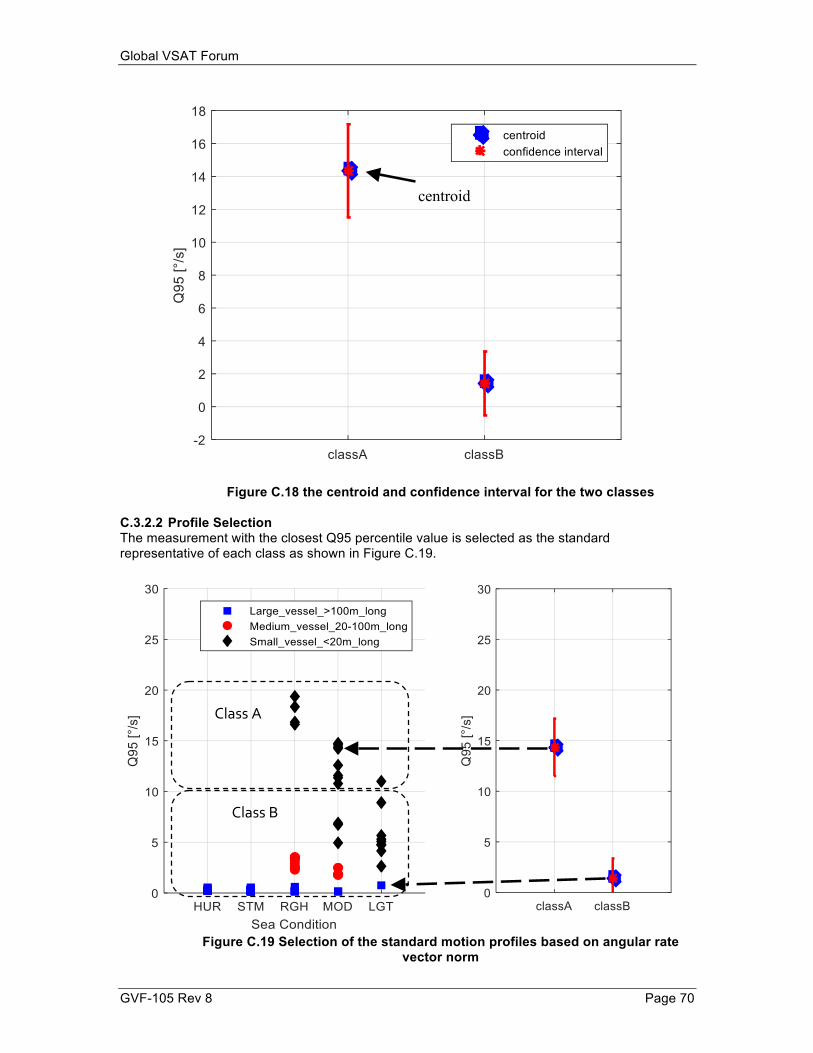
Global VSAT Forum

GVF-105 Rev 8

Figure C.18 the centroid and confidence interval for the two classes

C.3.2.2 Profile Selection The measurement with the closest Q95 percentile value is selected as the standard representative of each class as shown in Figure C.19.

Figure C.19 Selection of the standard motion profiles based on angular rate

vector norm

centroid

ClassB

ClassA

Global VSAT Forum

GVF-105 Rev 8

C.3.2.2.1 Class A standard Profile A motion track with a small vessel (KNRM lifeboat) on moderate sea conditions is selected for Class A. The CDF of the angular rates of the selected profile are shown in Figure C.20. The three individual axes, yaw, pitch and roll share in a balanced way to the overall motion dynamics. The selected profile is 15 minutes long. This is considered long enough to measure the dynamics performance of the terminal.

Figure C.20 the CDFs of the angular rates (vector norm and individual axes) of the class A

track

Global VSAT Forum

GVF-105 Rev 8

Figures C.21, C.22 and C.23 show the GPS data, satellite view and the vessel of the Class A profile, respectively.

Figure C.21: Class A profile -GPS profile-

Figure C.22: Class A profile –satellite top view-

Global VSAT Forum

GVF-105 Rev 8

Figure C.23: Class A vessel

C.3.2.2.2 Class B standard Profile Selecting the closest to the class B mean Q95 value leads to a motion profile which does not show balanced contribution of the individual axes to the overall motion dynamics. As plotted in Figure C.24, the yaw axis dominates. Moreover, the selected profile is only 2 minutes long. For a representative selection a longer profile is preferable. In order to have balanced excitation of the three individual axes, the measurement space around the mean Q95 value for class B was investigated. A measurement with a small vessel (KNRM lifeboat) on light sea conditions was showing balanced excitation for the individual axes. The profile is 5 minutes long. In order to get a longer profile (with 15 minutes to be of the same duration as in class A), the motion profile is repeated three consecutive times. It was ensured that the transitions between the repetitions are smooth such that the profiles do not have sudden jumps in the angular rates or accelerations. The CDFs of the final class B profile are shown in Figure C.25.

Global VSAT Forum

GVF-105 Rev 8

Figure C.24: CDF of the individual sub-axes of the initial selection of the Class B profile

the selected profile do not show balanced excitations for the individual axes

Figure C.25: CDF of the individual sub-axes of the final selection of the Class B profile the

selected profile show more balanced excitations for the individual axes compared to Figure C.24

Global VSAT Forum

GVF-105 Rev 8

Figures C.26, C.27 and C.28 show the GPS data, satellite view and the vessel of the Class B profile, respectively.

Figure C.26: Class B profile -GPS profile-

Figure C.27: Class B profile –satellite top view-

Global VSAT Forum

GVF-105 Rev 8

Figure C.28: Class B profile vessel

Global VSAT Forum

GVF-105 Rev 8

Appendix D: Literature [1] Technische Universität München – Institute of Astronautics in Co-operation with Eutelsat

Communications “Calculation of Azimuth, Elevation and polarization for non-horizontal aligned Antennas, Analytic Formulas”, Technical Document TD-1205-b

[2] H. Beljour, S. Foresta, et al. Army SATCOM OTM Full Elevation Performance Characterization. In The Military Communications Conference, 2011 [3] https://wermut.e-technik.tu-ilmenau.de/cmtn/main/portal/welcome [4] http://www.iis.fraunhofer.de/en/profil/standorte/forte.html [5] Gregor Siegert, Wolfgang Felber, Florian Raschke, Mostafa Alazab, Markus Landmann, “Advances of far field test range for SatCom On-the-Move terminals”, 7th Advanced Satellite Multimedia tems Conferenceand 13th Signal Processing for Space Communications Worshop, Sept.2014, Livorno, Italy [6] M. Alazab, M. Rieche, et al. On-Earth Performance Evaluation of SatCom On-the-Move (SOTM) Terminals, In The Military Communications Conference, 2013, San Diego, USA [7] M. Rieche, D. Arndt, A. Ihlow, and G. D. Galdo, “State modeling of the land mobile satellite channel by an image-based approach,” in 7th European Conference on Antennas and Propagation (EuCAP), Apr. 2013.

Global VSAT Forum

GVF-105 Rev 8

Appendix E: List of acronyms Acronyms utilized in this document are included in this appendix. Acronym Definition ASI Adjacent Satellite Interference - RF Energy radiated towards satellites adjacent to those intended for communication ATE Authorized Test Entity - An entity which performs verification tests in accordance with GVF authorization BER Bit Error Rate BPE Beam Pointing Error - error in earth terminal antenna pointing direction from desired direction CDF Cumulative Distribution Function COTM Communications On The Move - VSAT terminal capable of operating while mobile as well as in a fixed location. CW Continuous Wave EIRP Effective Isotropic Radiated Power EIRPSD Effective Isotropic Radiated Power Spectral Density - EIRP within a specific measurement bandwidth ETSI European Telecommunications Standards Institute FCC United States Federal Communications Commission FFT Fast Fourier Transform GSO Geo-Stationary Orbit IF Intermediate Frequency IMU Inertial Measurement Unit RF Radio Frequency - in this context, satellite uplink or downlink frequencies TDMA Time Division Multiple Access - an RF transmission scheme in which multiple transmissions are separated in time on a given RF frequency. QoS Quality of Service UDP User Datagram Protocol UPC Uplink Power Control - an automatic method of controlling uplink power in an earth terminal transmitter to compensate for changes in link losses, antenna radiation patterns, or other effects. USAT Ultra Small Aperture Terminal VMES Vehicle-Mounted Earth Station VSAT Very Small Aperture Terminal

Global VSAT Forumold.gvf.org/approvals/images/pdf/typeapprovalsdoc/GVF... · 2019-05-04 · Global...

Documents

Transcript of Global VSAT Forumold.gvf.org/approvals/images/pdf/typeapprovalsdoc/GVF... · 2019-05-04 · Global...