Global Trade, Contracts and Poverty Alleviation in ......the Nocheztlicalli: Museo Vivo de la Grana...

Global Trade, Contracts and Poverty Alleviation inIndigenous Communities:

Cochineal in MexicoPreliminary and incomplete

Alberto Diaz-CayerosUCSD

Saumitra Jha∗

Stanford GSB

July 5, 2012

Abstract

We explore the role played by contractual incentives generated by non-replicablefactors, high risk and costly verifiability in securing long term, sustained gains fromworld trade for indigenous communities. We examine the long term effects on in-digenous populations on cultivating one of the world’s most valuable traded com-modities: the “Spanish Red” dye extracted from the cochineal insect. We exploitthe discontinuous fragility of cochineal with respect to micro-climatic differencesduring the growing season to identify the effect of a legacy of cochineal production.We find that a legacy of cochineal production lowered the headcount poverty ratioin Mexican municipalities by 0.1, comparable to the entire effect of the Progressaconditional cash transfer program over a ten year period. Furthermore, cochinealproduction raised female literacy by 0.6 percentage points. Municipalities that con-tained pueblos that once produced cochineal are significantly more unequal, how-ever, have significantly fewer indigenous households and are less likely to formalizeindigenous local government institutions. We interpret these results as reflectingthe long-term effects of cochineal and the Repartimento contract that emerged tosupport the cochineal trade, provided opportunities to women and provided analternative to indigenous institutions as a means to manage risk.

∗Address: [email protected]; [email protected]. We would like to thank Sergio Juarez ofthe Nocheztlicalli: Museo Vivo de la Grana Cochinilla in Oaxaca for sharing his expertise on cochinealcultivation and Rodolfo Acuna and David Stahle for sharing their tree-ring reconstructions of historicalclimate. We are also grateful to Angeles Frizzi, Dorothy Kronick, Jessica Leino, Beatriz Magaloni andseminar participants at Stanford and in the US-Mexico conference on the Great Death for valuablecomments. Katrina Kosec provided excellent research assistance.

1

1 Introduction

Poor, disenfranchised or indigenous populations that live in regions with resources that

can be extracted for sale on world markets have long been seen as the accursed of global-

isation. Indeed, given the often dramatic differences in military and technological capa-

bilities between those seeking to acquire geographically-delimited resources and non-elite

indigenous populations that inhabit those areas, it is perhaps not surprising that this

is the case. Where such groups are able to employ the “weapons of the weak”, these

usually persist in marginal occupations that have relatively small gains (Scott, 1985).

Whether through violent coercion, the generation of inequality that results in oligarchic

political arrangements or due to the direct introduction by external actors of extractive

institutions, a large body of work suggests that openness to trade can lead indigenous

groups to face a long-term future of low growth and stunted development (Engerman and

Sokoloff, 2000, Acemoglu, Johnson, and Robinson, 2002, Nunn, 2008, Dell, forthcoming)

A related, but relatively unexplored aspect of the effects of openness on many indige-

nous communities lies in the replicability of their human capital, intellectual property

and natural resources. The ability to replicate and outsource the skilled production of

artisanal goods to lower-cost regions of the world has often meant that communities do

not benefit from world demand for goods researched and developed by their cultures over

centuries. Similarly, the ability of communities to gain from the exploitation of their

indigenous biological resources or processes of exploitation, such as spices, silkworms,

dyes or rubber, have often proved less durable sources of wealth as these processes and

goods are replicated elsewhere.1

Further, little empirical evidence is available on the conditions under which indige-

1For a description of the desolation of the Spice Islands following the transplantation of the nutmeg,see (Keay, 1991). On the importance of non-replicable sources of complementarity in supporting alegacy of inter-ethnic tolerance in South Asia, see Jha (2008b), and more generally, Jha (2008a).

An irony of being the originating region of biological resources is that the indigenous flora or faunaare often more difficult to cultivate there than in new areas– being indigenous, they also tend to havenatural predators that are absence elsewhere (Donkin, 1977)

2

nous societies are able to secure and sustain gains from indigenous human capital or

commodity trades valued by global demand over time, even in the absence of benign

third party intervention that could protect such gains. In this paper, we explore the role

played by contractual incentives generated by non-replicable factors, high risk and costly

verifiability in securing long term, sustained gains from world trade for indigenous com-

munities. We examine in particular the long term effects on indigenous populations on

cultivating one of the world’s most valuable traded commodities up until the late 19th

century: the “Spanish Red” dye extracted from the fragile cochineal insect. We per-

form this study in Mexico, a country where indigenous, colonial and modern identities

and institutions of governance have co-existed for centuries, and thus provides a useful

laboratory for understanding the long-term effects of trade on indigenous communities.

From the conquest of Mexico until the development of synthetic dyes in the late 1880s,

cochineal was the best source of red dye known to the West, and was highly prized in

the production of textiles, of which dyeing could constitute close to 40% of the overall

cost (Marichal, 2001). Crimsons and reds in particular were highly prized as colours

denoting status, both among the church and among royalty. Cochineal-dyed textiles,

further, were ten to twelve times more brilliant and remained fast compared to those of the

known alternatives derived from madder and the also-rare Mediterranean kermes (Lee,

1948, Marichal, 2001). As a result, from the 16th century to the independence of Mexico

in 1820, cochineal was also the most valuable processed good exported to Spain from the

Indies, second in value only to silver and gold. The average exports of cochineal between

1580-1600 were worth 550,000 pesos, close to 9% of the value of the silver exports from

New Spain (Lee, 1948). At its peak in 1771, cochineal had risen to be worth more than

4,200,750 pesos (Baskes, 2000).2

Fine cochineal – la grana cochinilla fina– was thus a highly prized commodity in

world trade. However, the domesticated cochineal insect also had one key distinguishing

2This price is based on the market price of cochineal in Oaxaca, near the main production areas ofcochineal. Naturally European prices would be considerably higher.

3

feature from other types of agricultural or mineral commodity: it was extremely fragile.

Unlike wild cochineal (cochinilla silvestre), fine cochineal only survived in regions with

particular combinations of precipitation, heat and cold. A sudden rain, frost or elevation

in temperature could kill the entire harvest (Donkin, 1977).

The fragility of cochineal had two effects: first, despite numerous attempts by Spain’s

rivals– England and France– it proved very difficult to transplant and replicate in experi-

mental farms outside of New Spain.3 Thus, unlike other prized agricultural commodities,

such as Brazilian rubber, Chinese silkworms or Indian indigo, cochineal was secure from

world competition and continued to prove a lucrative (New) Spanish monopoly for two

hundred and fifty years. Its fragility made cochineal much less transplantable and much

more localized in its production, in this sense, more like mineral resources than many

agricultural goods.

Second, because of its fragility, cochineal differed from mineral resources in that it

was both highly risky and required great care and attention to cultivate. Domesticated

cochineal had to be ‘seeded’ onto the paddles of the opuntia cactus. Immobile and

virtually defenseless itself, cochineal had also to be shielded from many potential threats.

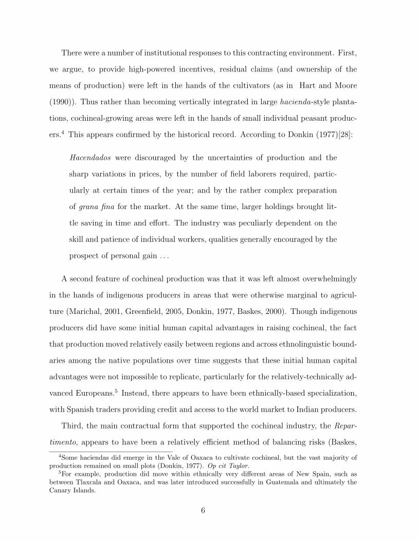
The 16th century chronicler of New Spain, Gonzalo Gomez de Cervantes devoted several

sections to cochineal, listing the “enemies” that ranged from wild cochineal and other

insects to the gusano tolero worm, and chickens and other birds that required constant

vigilance (Figure 1.)

We argue that the fragility of cochineal led both to the need for high-powered incen-

tives to care for the crop, as well as a basic problem of moral hazard or hidden action: it

was difficult for a principal to verify whether a cochineal crop had been destroyed due to

lack of effort, had been secretly sold on the market due to high prices or had been lost

due to the multiple natural threats that cochineal faced.

3French spies attempted to smuggle live cochineal to Haiti, while the English made similar attemptsat establishing cochineal plantations in India, but the cochineal insects were not to survive sea-bornetransplantation until the independence of Mexico and successful attempts by Spaniards to raise cochinealin the Canary Islands (Greenfield, 2005).

4

VOL. 67, PT. 5, 1977]

mm and a dry season of th!ree to four months were close to the minimum requirements.

The question whether D. coccus derives from a superior wild form which has now disappeared, or is a product of the improvement of one of the known wild species cannot be satisfactorily resolved. The notable differences between the present wild and cultivated forms at first suggest the former. Early commentators, however, generally assumed that the two were directly related, the differences being ascribed solely to cultivation.43 Certainly, the domestic Dactylopius is a deli- cate and vulnerable insect, closely dependent on man.

Improvement has come about through the selection and care of breeding populations, management of the host nopals, and partial protection from a large number of enemies, besides inclement weather. Gomez de Cer- vantes described in some detail the creatures that de- voured or attacked cochineal larvae and the immobile insects (fig. 3). They included turkeys and chickens

(gallinas de la tierra, gallinas de Castilla), birds generally, and various pests that called for constant sur- veillance-lizards (lagartijas), a kind of leech (sangui- juela), an insect "resembling a spider," 44 and several

grubs or worms (gusanos).45 Rats and mice arma- dillos, and some snakes were similarly harmful.46 In well-tended gardens, wild cochineal was removed,47 primarily to conserve the nopals and also to guard against interbreeding. The wild population must al-

ways have been kept severely in check by natural

enemies, and it is difficult to visualize an improved and

less robust species surviving at all. D. coccus tends

quickly to disappear when cultivation and protection cease.48 The differences between fina and silvestre forms appear to be largely the result of processes of

domestication operating over a considerable period of

time.

43Memorial (1620), 1931: p. 50 ("la silvestre fue el mismo genero que el de la fina y en la cultivacion esta la diferencia"). Discussed by Humboldt (1811: 3: pp. 65-66) and Dahlgren de Jordan (1963: p. 12).

44According to Diguet (1928: p. 520), spiders themselves were welcomed, chiefly because they fed on harmful insects, but not cochineal.

45 Gmez de Cervantes (1599), 1944: pp. 172-174. He also gives the Nahuatl names. Cf. Vasco (1776), 1963: p. 53; Magan (1776), 1963: p. 81.

46Clavijero (ca. 1780), 1964: p. 233; Alzate (1777-1794), 1852: p. 84; Humboldt, 1811: 3: p. 74. See also Leon Pinelo (1650), 1943: p. 248; Landivar (1781), 1948: p. 195; Dunlop, 1847: p. 130; Squier, 1858: p. 523; M. Herrera, 1919: p. 120.

47 Vasco (1776), 1963: p. 46; Magan (1776), 1963; p. 76; Alzate (1777-1794), 1852: pp. 84-85; Humboldt, 1811: 3: p. 75. Cf. Sahag6n (ca. 1570), 1938: 3: p. 288 (grana falsa, ixqui- miliuhqui).

48Alzate ([1777], 1794: p. 228) refers to the testimony of the alcade mayor of Nexapa (southern Oaxaca), according to which grana requisima was to be found, seven leagues or so from Nexapa, without cultivation, either of nopals or insects. This has no clear explanation, and falls short of proof of the existence, then or earlier, of a superior wild species.

FIG. 3. Enemies of cochineal. Gonzalo G6mez de Cervantes (1599), 1944.

CULTURE

The cycle of events associated with the cultivation of cochineal varied somewhat in different parts of the New World,49 chiefly according to the length and

49Remarked by Ulloa (1748), 1760: 1: pp. 341-347; but

COCHINEAL 15

Figure 1: Enemies of cochineal– Gonzalo Gomez de Cervantes (1599), La vidaeconomica y social de Nueva Espana el finalizar el siglo XVI , reproduced inDonkin (1977)

5

There were a number of institutional responses to this contracting environment. First,

we argue, to provide high-powered incentives, residual claims (and ownership of the

means of production) were left in the hands of the cultivators (as in Hart and Moore

(1990)). Thus rather than becoming vertically integrated in large hacienda-style planta-

tions, cochineal-growing areas were left in the hands of small individual peasant produc-

ers.4 This appears confirmed by the historical record. According to Donkin (1977)[28]:

Hacendados were discouraged by the uncertainties of production and the

sharp variations in prices, by the number of field laborers required, partic-

ularly at certain times of the year; and by the rather complex preparation

of grana fina for the market. At the same time, larger holdings brought lit-

tle saving in time and effort. The industry was peculiarly dependent on the

skill and patience of individual workers, qualities generally encouraged by the

prospect of personal gain . . .

A second feature of cochineal production was that it was left almost overwhelmingly

in the hands of indigenous producers in areas that were otherwise marginal to agricul-

ture (Marichal, 2001, Greenfield, 2005, Donkin, 1977, Baskes, 2000). Though indigenous

producers did have some initial human capital advantages in raising cochineal, the fact

that production moved relatively easily between regions and across ethnolinguistic bound-

aries among the native populations over time suggests that these initial human capital

advantages were not impossible to replicate, particularly for the relatively-technically ad-

vanced Europeans.5 Instead, there appears to have been ethnically-based specialization,

with Spanish traders providing credit and access to the world market to Indian producers.

Third, the main contractual form that supported the cochineal industry, the Repar-

timento, appears to have been a relatively efficient method of balancing risks (Baskes,

4Some haciendas did emerge in the Vale of Oaxaca to cultivate cochineal, but the vast majority ofproduction remained on small plots (Donkin, 1977). Op cit Taylor.

5For example, production did move within ethnically very different areas of New Spain, such asbetween Tlaxcala and Oaxaca, and was later introduced successfully in Guatemala and ultimately theCanary Islands.

6

2005). The standard contract was for the local Spanish official, the alcalde mayor, hav-

ing bid for the position and accumulated funding from Spanish merchants, to advance

12 pesos to indigenous producers for each pound of cochineal six months before har-

vest. This was considered a “fair” price”, and did not fluctuate much over time (Baskes,

2000)[62-92]. To the extent that cochineal producers were financed by the repartimento,

then the downside risk, and the exposure to world markets was borne by the alcalde

mayor (naturally, when self-financed, the risk was borne by the individual producers). In

practice however, when prices for cochineal were high, Indians would sell in markets and

claim that their harvests were destroyed. In his study of the cochineal contract, Jeremy

Baskes documents that this practice appears to be widespread. For example, the alcalde

mayor of Nexapa (1752) lamented:

that when market prices dropped he had no difficulty collecting the cochineal

owed to him, but that when prices were high debtors sold their stuff to trav-

eling merchants or in Antequera and later claimed to him that they lost their

harvests. The same was claimed by the alcalde mayor of Villa Alta, who in

1770 was unable to collect his cochineal debts from the Indians of his dis-

trict because, as he testified to the Viceroy, the prevailing high prices had

led debtors to renege on their contracted obligations and sell their output

elsewhere. In 1784, the alcalde mayor of Zimitlan-Chichicapa also noted the

propensity of Indians to abandon their obligations and sell elsewhere when

prices rose. Arij Ouweneel noted that the Indians of Puebla also “developed

a flair for the market” and bypassed their repartimento debts to the official

when market prices rose. . . ” (Baskes, 2000)[77].

In essence, therefore, the lack of ability to verify negative shocks to production re-

sulted in a contract where the indigenous population were insured against world market

fluctuations on the downside but possessed a call option through their ability to renege

on contracts, claim that the cochineal was destroyed and instead sell on the open market.

7

This maintained the high-powered incentives necessary for cultivating a risky crop, even

among the risk-averse poor.

A fourth feature of cochineal production was that it could be produced in small plots

near the home, and though it was labour-intensive, it did not require large degrees of

animal or human motive power. This provided particular possibilities for women and

children to engage in this lucrative activity, and indeed women and children were often

heavily involved in the cultivation of cochineal (Baskes, 2000). This may have altered

bargaining power within the household.

The strong relationship between indigenous identity and poverty, particularly in Mex-

ico and Latin America, has led to a long tradition which sees colonial institutions are

largely extractive and having deleterious effects on those communities. Similarly, the

Repartimento has long been seen as an exploitative contract, with Spanish traders as the

main beneficiaries. Though cochineal production in Mexico disappeared in the 19th cen-

tury, first with competition from Guatemala and the Canary Islands and then ultimately

with the synthesis of artificial dyes in the 1880s, historians have pointed to the relative

poverty and continued strength of the indigenous populations in cochineal-producing ar-

eas such as Oaxaca as indicative of the exploitative nature of the Repartimento and the

role of cochineal in maintaining indigenous identity, institutions and customs (Baskes,

2000, Greenfield, 2005).6 However there has been hitherto no attempt, to our knowledge,

to document the long term effects of these contractual arrangements on the indigenous

communities themselves.

In this paper, we exploit the fragility of cochineal with respect to micro-climatic dif-

ferences, using the discontinuous propensity to produce cochineal in areas that possess

the optimal raising conditions to areas just on the other side of these thresholds that

6 A recent reassessment by Baskes (2000) on the profitability of the Repartimento suggests that theindigenous communities were important beneficiaries of the Repartimento, while continuing to contendthat cochineal production led to the maintenance of indigenous identities and institutions. This islikely because Baskes’ focus is on the colonial period, when indigenous communities were the ones whobenefited from cochineal production.

8

lacked the right combination of precipitation and rainy season temperatures, to iden-

tify the effect of cochineal production on poverty, female literacy, inequality, indigenous

assimilation and the maintenance of usos y costumbres– traditional indigenous usages

and customs to manage local government. We find that a legacy of cochineal produc-

tion lowered the headcount poverty ratio in a municipality by around 0.1, a large value

comparable to the entire effect of the Progressa/ Opportunidades conditional cash trans-

fer program over a ten year period. Furthermore, cochineal production appears to have

raised female literacy by a remarkable 0.6 percentage points. Municipalities that con-

tained pueblos that once produced cochineal are significantly more unequal, however,

and, in a dramatic reversal from the 18th century, actually have significantly fewer in-

digenous households, and fewer who are monolingual in an indigenous language. They

are less likely to adopt indigenous local government institutions (usos y costumbres).

Public goods provision is generally as good however, apart from the provision of roads

and transport, which is considerably improved in cochineal producing areas.

We interpret these results as reflective of the long-term legacy of the repartimento

contract that underlied cochineal production in the colonial period. By providing access

to world markets and downside insurance, Spanish traders provided members of poor

indigenous communities, particularly women, a means to benefit from world trade and

to engage in market activity, leaving a beneficial legacy both on poverty reduction and

on women’s opportunities. However, because of the ability to exercise the “call option”,

renege on the repartimento contract and sell in markets when prices were high, the risky

nature of cochineal on the upside engendered inequality. Concurrently, Spanish offi-

cials had an incentive to build roads to cochineal producing areas to improve the ability

to access and monitor valuable goods for which they themselves were providing credit.

Despite cochineal production having initially safeguarded indigenous communities from

hacienda-isation and homogenization, increased inequality and access to market oppor-

tunities appears to have later undermined traditional (largely redistributive) political

9

institutions by leading first the richer and most mobile members to opt out and “his-

panicize”. Thus, part of the reason that indigenous communities appear poor in Latin

America and other areas may have less to do with colonial predation but instead precisely

because their most successful members chose to opt out and assimilate.

2 Empirical Strategy

In our empirical analysis, we will compare regions that possessed the optimal growing

conditions for cochineal to those that otherwise very similar to examine the effects of

cochineal in both geographical and climate space. We seek to identify the effect of past

cochineal production on contemporary measures of poverty, inequality, ethnic assimila-

tion, and the maintenance of traditional institutions. To do this, we will make two types

of comparison. First we will match cochineal producing areas to non-producing areas in

terms of their geography, in terms of climate, and both. The identifying assumption is

that the choice to produce cochineal in pueblos that are very close by to one another

in either (or both) geographic or climatic spaces was not shaped by unobserved initial

differences that also affect subsequent economic and political development.

In our benchmark specification, we will run cross-sectional regressions comparing

those municipalities that contained Indian pueblos in 1790.

yi = βCochineali +4∑j

γjGeogji +

2∑j

ξjClimji +XiB + εi (1)

Where yi is a set of 18th and 21st century measures of poverty, female literacy, ethnic

identity and public goods provision as well as whether the municipality has chosen to

explicitly adopt traditional governance institutions (usos y costumbres). Since only the

historically cochineal-growing state of Oaxaca has so far implemented laws recognizing

usos, we implement these specifications both for all Mexico and in Oaxaca only.

Cochineal is a measure of whether any pueblo within the municipality once produced

10

cochineal. We exploit a number of primary and secondary sources to identify the locations

of cochineal production, including a comprehensive search of all documents in the Archivo

General de Nueva Espana in Seville (please see data section).

Geogi is a vector of geographical initial conditions (higher order polynomials in lat-

itude, longitude and altitude). Climi is a set of climatic conditions– polynomials in

temperature and precipitation. We also include Xi- cultural initial conditions which

include distance to pre-Columbian native population or administrative centres and to

Conquest-period missions, arguably a good measure of the native population at the time

of the Conquest. We use robust standard errors.7

Though we attempt to identify all cochineal growing areas, there is a possibility that

Spanish colonial sources might have underestimated the extent to which cochineal was

grown in remote areas. To address this source of bias, we exploit the particular climactic

requirements of cochineal to compare areas that happen to be in the optimal growing

area for cochineal to generate a fuzzy discontinuity in geographical and climactic spaces.

As mentioned above, cochineal cultivation was highly dependent on favorable climac-

tic conditions. During the main growing season of March-August, the cochineal had to be

protected from precipitation (below 700mm was best) and large temperature variations

(i.e. frosts and temperatures above 30 C).8 The first stage regression is of the following

form:

Cochineali = ζOptimalClimi + +4∑j

γjGeogji +

2∑j

ξjClimji +XiB + νi (2)

By including the polynomials in geographical and climactic space, we are essentially

exploiting the discontinuity in the propensity to produce cochineal in some microclimates

7Clustering the standard errors at the modern province level does not affect the results substantively,but adds anachronism. A later version will report Conley standard errors to address potential spatialauto-correlation.

8Secondary sources do differ on the precise cutoffs– we follow Lee (1948). The ideal conditions forcochineal are 25C with very low precipitation (we thank Sergio Juarez, one of the two remaining modernproducers of cochineal in Oaxaca, for this observation.)

11

16 6

16.65

16.55

16.6

16.5

16 4

16.45

16.35

16.4

Puebla Reconstruction

16.3 Tlaxcala Reconstruction

16.25

1494

1508

1522

1536

1550

1564

1578

1592

1606

1620

1634

1648

1662

1676

1690

1704

1718

1732

1746

1760

1774

1788

1802

1816

1830

1844

1858

1872

1886

1900

1914

1928

1942

1956

1970

1984

1998

Figure 2: Temperature fluctuations in Tlaxcala and Puebla over 5 centuriesfrom tree-ring data.

compared to others that are right next to each other. While we should be using historical

climate, average temperatures have largely been preserved over the last four centuries at

least in two cochineal producing regions- Puebla and Tlaxcala- for which reliable tree-ring

reconstructions are possible (Figure 2).9

3 Data

We geographically identify 124 cochineal growing locations using a variety of colonial

sources. We relied primarily on the appendix compiled by Donkin (1977), which lists

9This is still a tentative conclusion. Though the preservation of the mean appears a robust conclusion,the calibration of the dendochronologies may not be precise, and it is possible that we should be usingthe second moment, and this is currently under research.

12

cochineal producing towns on the basis of the Matricula de Tributos for the precolonial

period; the Suma de Visitas for the early 16th century; the Relaciones Geograficas de

Indias for the late 16th Century; the Memoriales del Obispo de Tlaxcala by Alonso de la

Mota y Escobar for the 17th century; and B. Dahlgren de Jordan for the 18th century,

as well as some additional secondary sources.

We cross-examined this list by searching all ‘grana’ and ‘cochinilla’ mentions in Mex-

ico’s National Archives (the Archivo General de la Nacion, AGN), where we found 154

documents containing references to cochineal and specific town locations. There was

substantial overlap in the two listings.10

The sources we have used were explicitly designed by colonial administrators for the

purpose of identifying cochineal production and trade.11 Our data sources thus enable

us not only to identify cochineal growing regions, but also the specific century when

production was taking place.12

We geo-referenced all cochineal locations to their modern locality, using the Archivo

Historico de Localidades (AHL) produced by the Mexican National Statistical Institute,

INEGI.13 We failed to identify only 3 towns, which are not included in our dataset.

10We did not pursue around two dozen potential locations that are mentioned in AGN documents butare not in the more comprehensive colonial documents. We decided not to invest research resources onarchival work for those towns because the AGN documents are most likely mentions in passing of townsthat may not be growing cochineal or if they were, they are most likely small villages surrounding themain cochineal growing regions.

11For example, the Matricula de Tributos is an Aztec document that Cortez seized from Moctezuma,which identifies tributary provinces and towns, specifying cochineal taxed in kind by the Colohua-MexicaEmpire. The Suma de Visitas of 1548 was a census collected for tributary purposes, at a time whenIndian tribute was paid in kind, which allows for the identification of cochineal tribute paying places.The Relaciones Geograficas was a census ordered by Phillip II, explicitly asking in question 28 to report“the mines of gold, silver and other metals, and dyes that may exist in the town or its surroundings”.Dahlberg de Jordan’s source is the customs report of the port of Veracruz, identifying the producingtowns of cochineal exported during the late 18th century.

12Some of the Relaciones Geograficas of the late 16th century have been lost and that there might besome missing data for relevant growing regions in a given century, but we are quite confident that wehave included all the relevant towns where this activity existed in the colonial period, and if there areany missing towns, they are most likely in the immediate vicinity of the ones we have located.

13The AHL is a comprehensive geographic gazetteer that includes not only the modern place names,but variations in their spellings as well as brief references to the etymology and history of the towns.Due to changes in spelling and place names, as well as multiple modern possibilities with the same placename, we searched for confirmatory evidence to make sure we have identified the correct locality. Forexample, there are 10 modern localities in the state of Puebla with the name Acatlan, but we narrowed

13

In order to limit the range of our comparisons only to the territorial extent of the

settled areas of the New Spain we geographically identify the Indian pueblos and Spanish

cities ( ciudades and villas) at the end of the colonial period. We take advantage of the

georeferenced Atlas produced by Dorothy Tanck de Estrada, who geocoded the full range

of towns in New Spain at around 1790, the end of the colonial period. We matched each

of the more than 4500 pueblos in Tanck de Estrada (2005) to its modern locality.14 For

further details of the data, please see the Data Appendix.

4 Results

(Figure 3) overlays the conditions for cochineal growing with actual cochineal growing

among Indian pueblos, providing the 2-dimensional geographical equivalent of a univari-

ate regression discontinuity plot (Dell, forthcoming). Notice that pueblos that satisfy

none of the conditions were very unlikely to produce cochineal, while adding each con-

dition sequentially raises the likelihood of doing so, such that there is an additional,

discontinuous benefit from falling the optimal growing area. We can exploit each dis-

continuity separately as well as combine them into a single “optimal growing region”

variable. The results are consistent using either specification, though in what follows we

focus on the simple univariate specification.

As Table 1 reveals, the discontinuities in the graphical relationship in geographical

space are reflected in multivariate regressions of the propensity to produce cochineal in

the colonial period. Notice first that cochineal producing municipalities do not seem

to be systematically related to the level of pre-Columbian development as measured by

either proximity to pre-Columbian cities or to monasteries established at the time of

down the cochineal growing one to Acatlan de Osorio (INEGI code 210030001). Or a misspelled locationAhuatlan, Oaxaca, was identified as Miahuatlan de Porfirio Diaz (200590001).

14 Given that there is some uncertainty regarding externalities in the production of cochineal betweenlocalities, and that in urban areas pueblos have become part of larger metropolitan areas, we end upusing modern municipalities as the geographic units of analysis. Thus, instead of having around 2500municipalities, we restrict attention to 1700 municipalities that are relevant from the point of view ofthe colonial period.

14

E

E

E

E

E

EE E

E

E

E

E

E

EE

E

E

E

E

E

E

E

E

E

E

E

E

E

E

E

E

EE

E

E

E

E

E

E

E

E

E

E

E

E

E

E

E

E

E

EE

E

LegendDactylopius coccuspueblosindios

E spanishcity

Precip < 700mm, Mar-Aug

Max temp < 30C, Mar-Aug

Total Precipitation, Mar-AugValue

High : 2776Low : 7

Figure 3: Optimal growing conditions and cochineal production. Red dots denotecochineal (dactylopius coccus) producing locations in the colonial period. Green dotsdenote the locations of Indian towns (pueblos de indios) that existed in 1790. Darkerareas denote higher precipitation. Overlaid purple regions denote areas that satisfied allthree climactic conditions for growing cochineal.

15

the Conquest (arguably a measure of Conquest-era population densities (Diaz-Cayeros,

2010)). However, there is strongly significant and robust positive increase of around 3

to 5 percentage points of the presence of optimal growing conditions for cochineal on

whether a pueblo within the municipality was recorded as having grown cochineal in the

colonial period (1520-1820) (thus close to the mean propensity to produce cochineal of

around 5 percentage points). This is true controlling flexibly (using quadratic and quartic

specifications) for latitude, altitude and longitude (Cols 1-9) and comparing municipal-

ities within the same state (Cols 3-5,7-8). Cols 4-9 add polynomial controls for average

precipitation and temperature, but do not significantly alter the increase due to optimal

growing conditions.15

Subsetting the data to those municipalities within 100 km (62 miles) of the optimal

growing frontier halves the sample but yields very consistent results (Cols 6-8). Finally

comparing only those 451 municipalities within the cochineal-rich state of Oaxaca that

once had Indian pueblos raises the effect of the confluence of optimal growing conditions

on growing cochineal to around 10 percentage points.

Figure 4 shows an important outcome of interest– those municipalities designated

“poor” in 2001 and how they related spatially to the incidence of historical cochineal

production and climatic conditions, zooming into the poorer regions of Southern Mexico.

Notice that there are visible and striking differences among neighbouring municipalities,

with similar climatic conditions, that were considered poor and non-poor. Cochineal

producing municipalities often appear as islands of non-poverty in a relatively poor part

of the country.

These visible differences are also reflected in the effect of cochineal in reducing head-

count poverty ratio by around 10 percentage points and raising female literacy rates 5

percentage points seen in the OLS specifications in Table 2. Observe that these effects

are remarkably robust and stable across specifications, including matching in both geo-

15The F-test of the univariate instrument exceeds the Stock-Yogo criteria for weak instruments for anumber of specifications but can be improved upon.

16

E

E

E

E

E

E

E

E

E

E

E

E

E

E

E

E

E

E

E

E

EE

EE

E

E

E

E

E

E

E

E

E

E

LegendDactylopius coccus

E spanishcity




High : 2776Low : 7

Figure 4: Cochineal production and poor Southern Mexican municipalities(2001 CIMMYT data).

17

graphical and climatic space and comparing within municipalities within the same state

within 100km and 75km of the optimal growing frontier as well as within the state of

Oaxaca (Cols 1-9). The “fuzzy” regression discontinuity results (Cols 9-13) reveal broadly

consistent results in sign (and in the most tight comparisons (Cols 12-13), magnitude)

for poverty, though the effects are not precisely estimated. At the the same time, the

equivalent results on female literacy rates are unequivocally significant and robust: fe-

male literacy rates in regions that produced cochineal because they happened to fall in

the growing region are around 50 percentage points higher than those municipalities just

outside the region in both geographical and climate space (Cols 9-13).

The reduction in overall poverty and the rise in female literacy are consistent with two

features of the Repartimento contract that underlied cochineal production– the downside

insurance provided by Repartimento credit to poor farmers by providing a price floor for

cochineal, along with the role of cochineal in providing women in particular access to a

valued market activity. The relatively greater size of the fuzzy regression discontinuity

results are consistent with the possibility that we may be underestimating the location

of cochineal growing areas by using the actual mentions in colonial sources.

Historians have hypothesised that the small-scale cultivation of the cochineal and

the fact that land under cochineal production was mainly in the hands of indigenous

producers in the colonial period has had lasting effect on the maintenance of indigenous

identity and institutions (Greenfield, 2005, Baskes, 2000). Indeed, Oaxaca, Puebla and

Tlaxcala, three major cochineal producing states are also among the most ethnically

diverse.16 However, Table 3 shows the effect of a legacy of cochineal production on the

proportion of people in a municipality speaking an indigenous language, and decomposing

this figure into those that are monolingual and bilingual. A consistent picture emerges–

a legacy of cochineal production reduces the proportion speaking an indigenous language

16Cross-state evidence shows that these states also show relatively higher incidence of O- blood types,a blood type that is much more common among indigenous Mexicans than among those of Spanishorigins.

18

by 6 percentage points across OLS specifications. Furthermore, the effect is mainly to

reduce the number that are monolingual in an indigenous language in a municipality.

Even within poor, ethnically diverse Oaxaca, residents of municipalities who produced

cochineal as they were on the frontier of the optimal growing region were 0.56 percentage

points less likely to be monolingual (Panel C, Col. 13). Paradoxically, the residents of

cochineal-growing lands, despite having been left in the hands of indigenous producers

in the colonial period, have fewer residents that maintain a distinct indigenous linguistic

identity.

Table 4 suggests two reasons why this might be the case: cochineal producing mu-

nicipalities are now more unequal (Panel A), and also have greater access to the modern

road network (Panel B). Both of these effects are consistent with the Repartimento con-

tract and the incentives of global trade. The riskiness of cochineal production and the

“call option” that allowed cochineal producers to renege on the Repartimento contract

by selling cochineal at the market rate when prices were high is likely to lead to ex post

inequality. At the same time, access to cochineal-producing areas was valuable to Span-

ish local administrators, as this facilitated monitoring of contracts as well as reducing

the transportation costs of cochineal production. Since the local administrators were

themselves the main financiers of cochineal production, it is likely that the colonial road

network adapted itself towards cochineal producing areas. As noted above, cochineal

producing pueblos were not any closer on average to pre-Columbian sites. Furthermore,

lacking the need to design around Spanish-introduced mules, horses and in fact any

pack animal, pre-Columbian roads in Mexico tended to be superceded by a relatively

independently-created colonial road network that was built to link the newly-created

Spanish cuidades. However, Figure 5 shows road networks in 1790 (Gerhard, 1993) and

the network of paved roads today. While many Indian pueblos were bypassed, cochineal

producing pueblos appear to have been systematic beneficiaries of the expansion of the

road network, providing visual confirmation of Table 4(Panel B).

19

The presence of increased inequality and ease of access to outside opportunities pro-

vides an explanation for the decline of indigenous identity and the relative assimilation

of cochineal-producing areas, when combined with a third factor– that those that com-

mitted to maintaining an indigenous identity also were more likely to have pay into often

highly redistributive indigenous governance institutions. These governance institutions,

while potentially playing an important risk-sharing role in many communities, are likely

to less important in an environment where Repartimento contracts for cochineal provided

risk insurance (and reduced poverty) instead. On the other hand, increased inequality

and ease of mobility is likely to have encouraged the most productive members “opt”

out by hispanicizing.17 Indeed, as Panel C, suggests, cochineal producing municipalities,

both exploiting cross-state variation and looking within Oaxaca, were much less likely

to opt for formalizing the use of highly redistributive indigenous governance institutions

(usos y costumbres).

Despite having failed to maintain indigenous governance, as Table 5 reveals, munic-

ipalities with a legacy of producing cochineal are at least as good as nearby areas at

providing public goods such as water, electricity and drains to their populations. Thus

it appears that increased inequalities and the failure to maintain traditional institutions

have not had a deleterious effect on these indicators of development.

5 Conclusion

World trade has not treated most indigenous communities well. The members of such

communities often number among the poorest and most vulnerable. Despite the benefits

that world trade should confer in principle, the conditions under which indigenous com-

munities with replicable human capital or expropriable resources can benefit over the long

term from openness to trade have not been adequately explored. In this paper, we pro-

17This logic has clear parallels to the decision of productive members to opt out of the highly-redistributive Israeli Kibbutz (see Abramitzky (2008)).

20

vide an example where indigenous communities succeeded in wresting a share of the gains

from trade over more than two centuries, leaving a lasting legacy of reduced poverty and

improved female literacy. At the same time, access to the contracts that supported the

trade appear to have changed the communities themselves, providing individuals alterna-

tive means to mitigate risk that appear to have undermined local indigenous governance

institutions and encouraged broader assimilation. In this way, successful and sustained

gains from trade may have led indigenous communities to cease being indigenous. The

relationship between indigenous identity and poverty visible throughout Latin America

then may be due in part to the “opting out” of those successful at securing the gains

from globalization.

Our example of an instance where indigenous communities gained from openness to

globalization does however raise the issue of the special nature of the conditions under

which poor indigenous societies can protect their intellectual property and expropriable

resources in the absence of benign third party enforcement. The unusual fragility of

cochineal, that made it difficult to transplant, in combination with the need for high-

powered incentives to encourage cultivation, was not characteristic of many other forms

of intellectual property, human capital or resources. Indeed, the entrepreneurial spirit of

colonial administrators in transplanting indigenous crops and techniques researched and

developed over centuries throughout their empires, while fostering world trade in the 18th

and 19th centuries, may have also played a major role in providing indigenous societies

with nothing to sell and thus little to bargain with when confronted by globalization.

21

E

E

E

E

E

E E

E

E

E

LegendDactylopius coccus

E spanishcity

Caminos, 1790

roads

TYPEDivided Highway

Undivided Highway

Paved Road

Unimproved

pueblosindios




High : 2776Low : 7

Figure 5: Cochineal production and the evolution of road networks in South-ern Mexico. The light blue lines denote the road networks of New Spain (1790), asdocumented by Gerhard (1993). The red lines represent modern roads.

22

6 Data Appendix

For the vector of geographic conditions we use latitude, longitude and altitude. Longi-

tude and latitude are measured in degrees, calculated at the geographic centroid of each

municipality using ArcGIS. Altitude is calculated as the average of each municipality,

measured in meters, using the Digital Elevation Model with a horizontal grid spacing of

30 arc seconds (approximately 1 kilometer) produced by the US Geological Survey EROS

Data Center.

For the climatic data we have used two distinct data sources. For each municipality

we calculated the average rainfall and temperature according, to the official climatology

maps of the Mexican National Statistical Office, INEGI. The data was collected from

meteorological stations from 1921 to 1975 and processed in 2000. For the monthly data

on precipitation we used a 30 arc second resolution database from Worldclim, version

1.4, interpolated by Hijmans, Cameron, Parra, Jones, and Jarvis (2005). The monthly

data is calculated for the 1950-2000 period. This monthly data is used to restrict the

optimal cochineal growing regions as those that during the main growing season (March

to August) are always below 700 mm and did not experience frosts and temperatures

above 30 degrees Celsius.

To control for the initial conditions before the colonial period, we have calculated hiker

distances to the main archeological sites that were developed before the conquest and

the hiker distance to the network of missions established by the Dominican, Augustine

and Franciscan religious orders during the 16th century. These topographic distances

are averaged over the municipality. Hiker distances are used because the available means

of transportation without horses or mules meant that the network of urban settlements

and transportation corridors was connected through trails that followed the valleys and

areas of relatively easy access. We use the most important archeological sites, which are

the 170 sites open to the public.

Given the high mortality that characterized the 16th century we cannot use population

23

headcounts during the first century of contact as a measure of population density or

settlement patterns. Those population figures most likely reflect differential mortality

rates across pueblos. Instead, we use the network of missions, which gives us a proxy for

the population density and the network that connected Indian society before the time of

contact. The three religious orders competed during the 16th century seeking to place

their missions in the places where they could maximize Christianization and access to

Indian communities. The geocoding of missions is made on the basis of the maps provided

by Kubler (1948). Details on the calculation of hiker distances, which use the slope of

the terrain, can be found in Diaz-Cayeros (2010).

The data used for the contemporary measures of development, ethnic composition,

inequality and local public goods provision we calculate the following indicators from

official INEGI 2000 census data:

Female literacy rates (Alfamujeres): women over 12 years old who cannot read or

write. Indigenous : percent of municipal inhabitants over 5 years old who speak an in-

digenous language. Bilingual : percent of municipal inhabitants over 5 years old who

speak Spanish and an indigenous language. Monolingual : percent of municipal inhab-

itants over 5 years old who speak an indigenous language but do not speak Spanish.

Inequality : Gini coefficients calculated by Jensen and Rosas (2007) on the basis of the

household income reported in the census, measured as multiples of the minimum wage.

Distance to roads is calculated as the Euclidean distance to the main roads as of 2000

from INEGI, calculated with ArcGIS.

Usos y Costumbres is a dummy variables denoting the municipalities that elect mayors

through traditional methods instead of partisan elections. The source for this data is the

Electoral Institute of Oaxaca.

Poverty headcount ratio (paliha) is a poverty headcount at the municipal level calcu-

lated by the Mexican Commission for Social Evaluation (CONEVAL) on the basis of a

small area estimation using the 2002 income distribution survey (ENIGH) and the 2000

24

census.

References

Abramitzky, R. (2008): “Limits of Equality: Lessons from the Israeli Kibbutz,” Quar-terly Journal of Economics, pp. 1111–1159.

Acemoglu, D., S. Johnson, and J. A. Robinson (2002): “Reversal of fortune:geography and institutions in the making of the modern world income distribution,”Quarterly Journal of Economics, 117, 1231–1294.

Baskes, J. (2000): Indians, merchants and markets: a reinterpretation of the Reparti-mento and Spanish-Indian economic relations in colonial Oaxaca, 1750-1821. StanfordUniversity Press.

(2005): “Colonial institutions and cross-cultural trade: Repartimento credit andindigenous production of cochineal in eighteenth century Oaxaca, Mexico,” Journal ofEconomic History, 65(1), 186–210.

Dell, M. (forthcoming): “The Persistent Effects of Peru’s Mining Mita,” Econometrica.

Diaz-Cayeros, A. (2010): “Indian identity, poverty and colonial development in Mex-ico,” Paper presented at Stanford.

Donkin, R. (1977): “Spanish Red: An Ethnogeographical Study of Cochineal and theOpuntia Cactus,” Transactions of the American Philosophical Society, 67(5), 1–84.

Engerman, S. L., and K. L. Sokoloff (2000): “Institutions, factor endowments andpaths of development in the New World,” Journal of Economic Perspectives, 14(3),217–32.

Gerhard, P. (1993): A guide to the historical geography of New Spain. University ofOklahoma Press.

Gomez de Cervantes, G. (1599): La vida economica y social de Nueva Espana elfinalizar el siglo XVI. 1944 edn.

Greenfield, A. B. (2005): A Perfect Red: Empire, espionage and the quest for thecolor of desire. HarperCollins, New York, 2006 edition edn.

Hart, O., and J. Moore (1990): “Property rights and the nature of the firm,” Journalof Political Economy, 98, 1119–58.

Hijmans, R., S. Cameron, J. Parra, P. Jones, and A. Jarvis (2005): “Very highresolution interpolated climate surfaces for global land areas,” International Journalof Climatology, 25, 1965–1978.

Jensen, N. M., and G. Rosas (2007): “Foreign Direct Investment and Income In-equality in Mexico, 1990-2000,” International Organization, 61(3), 467–487.

25

Jha, S. (2008a): “A theory of trade, ethnic cronyism and tolerance,” Stanford GSB(mimeo).

(2008b): “Trade, institutions and religious tolerance: evidence from India,”GSB Research Paper 2004, Stanford Graduate School of Business, Stanford CA.

Keay, J. (1991): The Honourable Company: a history of the English East India Com-pany. Macmillan, New York, NY.

Kubler, G. (1948): Mexican Architecture in the Sixteenth Century. Yale UniversityPress, New Haven.

Lee, R. (1948): “Cochineal Production and Trade in New Spain to 1600,” The Americas,4(4), 449–473.

Marichal, C. (2001): “A forgotten chapter of international trade: Mexican cochinealand European demand for American dyes, 1550-1850,” Paper presented to the Confer-ence on “Latin America Global Trade”, Stanford.

Nunn, N. (2008): “The Long Term Effects of Africa’s Slave Trades,” Quarterly Journalof Economics, 123(1), 139–176.

Scott, J. (1985): Weapons of the weak: everyday forms of peasant resistance. YaleUniversity Press.

Tanck de Estrada, D. (2005): Atlas ilustrado de los pueblos de indios : NuevaEspana, 1800. Colegio de Mexico.

26

Tab

le1:

Regre

ssio

n:

Coch

ineal

inth

eco

lonia

lp

eri

od

Mun

icipalities con

taining 17

90 pue

blos only

(1)

(2)

(3)

(4)

(5)

(6)

(7)

(8)

(9)

OLS

OLS

State FE

State FE

State FE

<100

kmState FE,

<100

kmState FE,

<100

kmOaxaca

only

Optim

al growing cond

ition

s in m

unicipality

0.04

1***

0.04

7***

0.03

7***

0.03

5***

0.03

1**

0.03

1*0.03

0*0.03

7**

0.10

3**

[0.014

][0.014

][0.014

][0.013

][0.014

][0.017

][0.017

][0.018

][0.042

]ik

'di

lbi

ik

Hiker's distance to pre‐Colum

bian

site

s, 100

0km

0.10

70.02

40.07

00.02

00.04

8‐0.060

0.25

70.18

90.06

8[0.134

][0.141

][0.145

][0.137

][0.144

][0.236

][0.264

][0.261

][0.299

]Hiker's distance to m

onasteries (1

6C), 10

00km

‐0.064

‐0.016

‐0.117

‐0.114

‐0.181

0.12

1‐0.373

‐0.428

‐0.116

[0.115

][0.123

][0.131

][0.126

][0.134

][0.242

][0.275

][0.271

][0.370

]Average precipitatio

n (m

)0.02

6***

0.02

6***

0.02

50.03

2*0.02

7*0.04

6***

[000

7][0

008]

[001

6][0

016]

[001

6][0

017]

[0.007

][0.008

][0.016

][0.016

][0.016

][0.017

]

Average precipitatio

n2‐0.003

***

‐0.003

***

‐0.003

‐0.004

‐0.003

‐0.004

*[0.001

][0.001

][0.003

][0.003

][0.003

][0.003

]

Tempe

rature (o C)

0.00

7*0.00

9**

0.00

9*0.00

9*0.00

9*0.01

8[0.004

][0.004

][0.005

][0.005

][0.005

][0.012

]

Tempe

rature

20.00

0‐0.000

*0.00

0‐0.000

*0.00

00.00

0[0.000

][0.000

][0.000

][0.000

][0.000

][0.000

]Quadratic in

Lat, Lon

g, Altitude

YY

YN

YY

YY

YQuartic in

Lat, Lon

g, Altitude

NY

NN

NN

NY

NF‐test (O

ptim

al Growing = 0)

9.11

10.91

7.15

6.83

5.37

3.15

3.11

4.38

5.89

(p

g)

Prob

>F0.00

0.00

0.01

0.01

0.02

0.08

0.08

0.04

0.02

Observatio

ns17

0717

0717

0717

1717

0797

597

597

545

1R‐squared

0.04

0.05

0.05

0.06

0.06

0.06

0.08

0.09

0.05

Sample restricted

to m

unicipalities con

taining 17

90 pue

blos de los indios. R

obust stand

ard errors in

brackets; * significant a

t 10%

; ** significant at 5

%; ***

significant

at1%

;Note:``<100

km''represen

tsthosemun

icipalities

with

in10

0km

oftheop

timalgrow

ingregion

fron

tier.Thisisapprox.62miles.

significant at 1

%; N

ote: <100

km rep

resents those mun

icipalities with

in 100

km of the

optim

al growing region

fron

tier. This is app

rox. 62 miles.

27

Tab

le2:

Regre

ssio

n:

Povert

yand

Fem

ale

Lit

era

cy

(1)

(2)

(3)

(4)

(5)

(6)

(7)

(8)

(9)

(10)

(11)

(12)

(13)

OLS,

State FE

OLS,

State FE

OLS,

State FE

OLS,

State FE,

<100

km

OLS,

State FE,

<75km

OLS,

State FE,

<100

km

OLS,

State FE,

<75km

OLS,

Oaxaca

only

2SLS‐RD,

State FE

2SLS‐RD,

State FE

2SLS‐RD,

State FE,

<100

km

2SLS‐RD,

State FE,

<75km

2SLS‐RD,

Oaxaca

only

Pane

l A: P

overty Headcou

nt Ratio (P

aliha)

Cochineal produ

cer

‐0.101

***

‐0.107

***

‐0.105

***‐0.124

***

‐0.128

***

‐0.120

***

‐0.121

***

‐0.126

***

‐0.586

*‐0.501

0.03

4‐0.092

‐0.159

[0.022

][0.022

][0.022

][0.025

][0.026

][0.025

][0.026

][0.028

][0.352

][0.397

][0.266

][0.250

][0.221

]Hiker's distance to pre‐Colum

bian

site

s, 100

0km

0.74

5***

0.87

6***

0.74

1***

1.08

9***

1.09

4***

1.10

1***

1.12

3***

0.88

2***

0.69

3***

0.69

3***

0.95

5***

1.02

7***

0.72

0***

[0.105

][0.104

][0.104

][0.177

][0.185

][0.181

][0.189

][0.156

][0.128

][0.120

][0.192

][0.193

][0.156


onasteries (1

6C), 10

00km

1.06

8***

0.76

0***

0.94

7***

0.83

9***

0.86

7***

0.85

4***

0.89

2***

0.42

5***

1.03

2***

0.91

5***

0.98

1***

0.93

6***

0.54

3***

[0.101

][0.102

][0.107

][0.200

][0.209

][0.204

][0.214

][0.162

][0.132

][0.144

][0.236

][0.238

][0.189

]Observatio

ns17

6317

7817

6310

1193

310

1193

348

517

0717

0797

590

245

1R‐squared

0.59

0.59

0.59

0.63

0.63

0.63

0.63

0.31

0.45

0.5

0.63

0.65

0.32

Pane

l B: W

omen

's literacy rate (Alfa

Mujeres)

Cochineal produ

cer

0.05

0***

0.05

2***

0.05

0***

0.06

8***

0.06

6***

0.06

3***

0.05

9***

0.06

1***

1.19

3***

1.21

6**

0.57

2**

0.50

7**

0.64

0**

[0.012

][0.012

][0.012

][0.013

][0.014

][0.013

][0.014

][0.019

][0.462

][0.544

][0.239

][0.223

][0.291


bian

site

s, 100

0km

‐0.323

***

‐0.390

***

‐0.332

***‐0.527

***

‐0.561

***

‐0.534

***

‐0.576

***

‐0.174

‐0.338

*‐0.328

*‐0.579

***

‐0.581

***

‐0.111

[0.077

][0.073

][0.077

][0.130

][0.131

][0.133

][0.133

][0.135

][0.183

][0.183

][0.204

][0.191

][0.215


onasteries (1

6C), 10

00km

‐0.517

***

‐0.346

***

‐0.435

***

‐0.166

‐0.126

‐0.199

‐0.159

‐0.218

‐0.392

**‐0.256

‐0.02

‐0.014

‐0.08

[0.071

][0.071

][0.076

][0.141

][0.143

][0.143

][0.143

][0.155

][0.168

][0.188

][0.218

][0.210

][0.275

]Observatio

ns17

6317

7817

6310

1193

310

1193

348

517

0717

0797

590

245

1R‐squared

0.48

0.48

0.48

0.48

0.47

0.49

0.48

0.2

Quadratic in

Lat, Lon

g, Altitude

YN

YY

YY

YY

YY

YY

YQuadratic in

Precipitatio

n and Tempe

rature

NY

YY

YY

YY

NY

YY

YQuartic in

Lat, Lon

g, Altitude

NN

NN

NY

YN

NN

YY

N

Sample restricted

to m

unicipalities con

taining 17

90 pue

blos de indios. R

obust stand

ard errors in


t 10%


%; ***

significant a

t 1%; N

ote: ``<100

km'' (75km)

represen

ts th

ose mun

icipalities with

in 100

km (7

5km) o

f the

optim

al growing region

fron

tier. This is app

rox. 62 miles (47 miles)

28

Tab

le3:

Regre

ssio

n:

Indig

enous

Language

Use

(1)

(2)

(3)

(4)

(5)

(6)

(7)

(8)

(9)

(10)

(11)

(12)

(13)

OLS,

State FE

OLS,

State FE

OLS,

State FE

OLS,

State FE,

<100

km

OLS,

State FE,

<75km

OLS,

State FE,

<100

km

OLS,

State FE,

<75km

OLS,

Oaxaca

only

2SLS‐RD,

State FE

2SLS‐RD,

State FE

2SLS‐RD,

State FE,

<100

km

2SLS‐RD,

State FE,

<75km

2SLS‐RD,

Oaxaca

only

Pane

l A: %

spe

aking an

indigeno

us langua

geC

hil

d006

7**

007

0**

005

9**

005

9*005

0005

2004

0006

5356

8**

358

4**

173

5**

146

0**

146

0*Co

chineal produ

cer

‐0.067

**‐0.070

**‐0.059

**‐0.059

*‐0.050

‐0.052

‐0.040

‐0.065

‐3.568

**‐3.584

**‐1.735

**‐1.460

**‐1.460

*[0.028

][0.029

][0.028

][0.032

][0.034

][0.032

][0.034

][0.042

][1.386

][1.615

][0.718

][0.655

][0.757


bian

site

s, 100

0km

0.44

3**

0.73

3***

0.49

9***

0.35

50.52

9*0.49

30.70

1**

0.65

3**

0.45

10.43

70.80

90.80

30.41

7[0.178

][0.179

][0.175

][0.299

][0.309

][0.301

][0.310

][0.329

][0.536

][0.535

][0.566

][0.520

][0.523


onasteries (1

6C), 10

00km

1.34

3***

0.64

3***

1.13

0***

1.03

0***

0.82

4***

0.97

3***

0.75

0**

1.45

5***

0.95

5*0.57

40.24

90.24

61.09

0[0.165

][0.176

][0.173

][0.309

][0.316

][0.304

][0.308

][0.367

][0.493

][0.542

][0.606

][0.566

][0.669

]Observatio

ns17

6317

7817

6310

1193

310

1193

348

517

0717

0797

590

245

1Observatio

ns17

6317

7817

6310

1193

310

1193

348

517

0717

0797

590

245

1R‐squared

0.42

0.39

0.44

0.34

0.33

0.36

0.35

0.26

Pane

l B: %

bilingua

l in Span

ish an

d an

indigeno

us langua

geCo

chineal produ

cer

‐0.038

‐0.041

*‐0.032

‐0.031

‐0.027

‐0.026

‐0.020

‐0.033

‐2.367

**‐2.363

**‐1.316

**‐1.103

**‐0.883

*[0.024

][0.025

][0.024

][0.027

][0.029

][0.028

][0.030

][0.034

][0.940

][1.091

][0.558

][0.509

][0.516


bian

site

s, 100

0km

0.35

2***

0.56

2***

0.39

0***

0.21

40.36

10.31

10.48

3*0.56

7**

0.34

40.33

80.55

90.56

00.37

0[0.131

][0.134

][0.130

][0.236

][0.245

][0.238

][0.247

][0.245

][0.360

][0.358

][0.433

][0.401

][0.354


onasteries (1

6C), 10

00km

0.87

7***

0.35

6***

0.73

1***

0.86

6***

0.69

5***

0.83

1***

0.64

7***

1.11

6***

0.61

6*0.35

70.26

30.25

50.90

1**

[0.116

][0.125

][0.121

][0.243

][0.250

][0.240

][0.244

][0.264

][0.331

][0.362

][0.464

][0.435

][0.447

]Observatio

ns17

6317

7817

6310

1193

310

1193

348

517

0717

0797

590

245

1R‐squared

0.44

0.41

0.45

0.35

0.34

0.37

0.35

0.25

Pane

lC:%

mon

olingualinan

indigeno

uslangua

gePa

nel C: %

mon

olingual in

an indigeno

us langua

geCo

chineal produ

cer

‐0.028

***

‐0.028

***

‐0.026

***‐0.027

***

‐0.022

***

‐0.025

***

‐0.020

***

‐0.031

**‐1.164

***

‐1.183

**‐0.400

**‐0.346

**‐0.560

**[0.008

][0.008

][0.008

][0.007

][0.007

][0.007

][0.007

][0.013

][0.446

][0.525

][0.177

][0.163

][0.277


bian

site

s, 100

0km

0.08

50.16

4***

0.10

20.12

50.15

3*0.16

5*0.20

2**

0.08

10.10

00.09

20.23

00.22

5*0.04

3

[0.066

][0.063

][0.066

][0.087

][0.087

][0.089

][0.089

][0.128

][0.178

][0.179

][0.144

][0.134

][0.199


onasteries (1

6C), 10

00km

0.44

5***

0.27

4***

0.38

1***

0.16

7*0.13

30.14

30.10

60.32

9**

0.32

3*0.20

5‐0.005

‐0.002

0.18

4[0

069]

[006

9][0

073]

[009

0][0

089]

[009

0][0

087]

[016

0][0

165]

[018

3][0

150]

[014

2][0

264]

[0.069

][0.069

][0.073

][0.090

][0.089

][0.090

][0.087

][0.160

][0.165

][0.183

][0.150

][0.142

][0.264

]Observatio

ns17

6317

7817

6310

1193

310

1193

348

517

0717

0797

590

245

1R‐squared

0.25

0.23

0.26

0.21

0.19

0.23

0.21

0.18

Quadratic in

Lat, Lon

g, Altitude

YN

YY

YY

YY

YY

YY

YQuadratic in

Precipitatio

n and Tempe

rature

NY

YY

YY

YY

NY

YY

YQuartic in

Lat, Lon

g, Altitude

NN

NN

NY

YN

NN

YY

N

Samplerestricted

tomun

icipalities

containing

1790

pueb

losde

indios

Robu

ststandard

errorsinbrackets;*significant

at10

%;**significant

at5%

;***

significant

at1%

;Note:``<100

km''(75km)

Sample restricted

to m

unicipalities con

taining 17

90 pue

blos de indios. R

obust stand

ard errors in


t 10%


%; ***

significant a

t 1%; N

ote: ``<100

km'' (75km)

represen

ts th

ose mun

icipalities with

in 100

km (7

5km) o

f the

optim

al growing region

fron

tier. This is app


29

Tab

le4:

Regre

ssio

n:

Inequali

tyand

Indig

enous

Govern

ance

(1)

(2)

(3)

(4)

(5)

(6)

(7)

(8)

(9)

(10)

(11)

(12)

(13)

OLS,

State FE

OLS,

State FE

OLS,

State FE

OLS,

State FE,

<100

km

OLS,

State FE,

<75km

OLS,

State FE,

<100

km

OLS,

State FE,

<75km

OLS,

Oaxaca

only

2SLS‐RD,

State FE

2SLS‐RD,

State FE

2SLS‐RD,

State FE,

<100

km

2SLS‐RD,

State FE,

<75km

2SLS‐RD,

Oaxaca

only

Pane

l A: G

ini coe

fficient

Chi

ld

002

2***

002

1***

002

1***

001

8***

001

8**

001

9***

001

9***

002

2***

027

8**

026

6*013

1009

3010

4Co

chineal produ

cer

0.02

2***

0.02

1***

0.02

1***

0.01

8***

0.01

8**

0.01

9***

0.01

9***

0.02

2***

0.27

8**

0.26

6*0.13

10.09

3‐0.104

[0.006

][0.006

][0.006

][0.007

][0.007

][0.007

][0.007

][0.008

][0.138

][0.159

][0.091

][0.085

][0.094


bian

site

s, 100

0km

‐0.104

***

‐0.116

***

‐0.113

***

‐0.046

‐0.02

‐0.06

‐0.041

‐0.208

***

‐0.116

**‐0.116

**‐0.091

‐0.069

‐0.239

***

[0.039

][0.037

][0.039

][0.062

][0.064

][0.064

][0.066

][0.065

][0.054

][0.053

][0.071

][0.070

][0.080


onasteries (1

6C), 10

00km

0.19

1***

0.22

1***

0.20

3***

0.27

3***

0.25

7***

0.28

7***

0.27

6***

0.08

40.21

8***

0.24

3***

0.32

9***

0.31

4***

0.04

2[0.037

][0.035

][0.038

][0.067

][0.069

][0.069

][0.071

][0.073

][0.051

][0.056

][0.079

][0.076

][0.093

]Observatio

ns17

6317

7817

6310

1193

310

1193

348

517

0717

0797

590

245

1Observatio

ns17

6317

7817

6310

1193

310

1193

348

517

0717

0797

590

245

1R‐squared

0.19

0.18

0.19

0.24

0.25

0.25

0.26

0.16

Pane

l B: D

istance to m

ajor 21st cen

tury roa

ds (k

m)

Cochineal produ

cer

‐2.031

**‐2.120

***

‐1.966

**‐1.907

**‐1.849

**‐2.044

***

‐1.973

**‐1.553

‐72.91

7**

‐79.77

4**

‐16.05

4‐8.208

‐55.23

9**

[0.810

][0.800

][0.803

][0.786

][0.800

][0.791

][0.805

][1.090

][30.40

6][38.11

6][12.05

0][11.95

3][25.22

5]Hiker's distance to pre‐Colum

bian

site

s, 100

0km

35.639

***42

.437

***36

.743

***32

.037

***31

.118

***27

.326

***26

.362

***78

.527

***35

.922

***34

.979

***27

.700

***23

.729

***73

.168

***

[5.936

][5.770

][5.875

][7.781

][8.207

][7.198

][7.479

][7.422

][12.04

5][12.81

9][8.148

][7.654

][17.84

7]Hiker's distance to m

onasteries (1

6C), 10

00km

15.449

**9.36

413

.981

**18

.423

**16

.055

*18

.298

**15

.866

*1.72

57.98

32.35

213

.926

17.185

*‐11.88

7[6.183

][6.673

][6.423

][8.506

][8.815

][8.648

][9.076

][10.18

3][11.62

9][13.72

6][10.06

6][10.10

7][23.73

6]Observatio

ns17

6317

7817

6310

1193

310

1193

348

517

0717

0797

590

245

1R‐squared

0.27

0.26

0.27

0.34

0.33

0.38

0.37

0.44

Pane

lC:M

unicipalityad

optedindigeno

uslocalgoverna

nceinstitutions

(UsosyCo

stum

bres

)Pa

nel C: M

unicipality ad

opted indigeno

us local governa

nce institutions (Usos y Co

stum

bres

)Co

chineal produ

cer

‐0.515

***

‐0.477

***

‐0.500

***‐0.525

***

‐0.533

***

‐0.529

***

‐0.532

***

‐0.819

***

2.10

81.15

5‐0.069

0.33

42.68

2[0.149

][0.154

][0.149

][0.183

][0.193

][0.184

][0.194

][0.222

][1.677

][1.720

][4.017

][1.322

][2.282


bian

site

s, 100

0km

3.85

1***

4.22

6***

3.78

3***

1.42

51.16

01.43

21.17

97.40

8***

3.80

8***

3.83

3***

1.54

71.35

67.52

1***

[0.606

][0.641

][0.614

][1.024

][1.054

][1.036

][1.066

][1.280

][0.713

][0.661

][1.138

][1.102

][1.692


onasteries (1

6C), 10

00km

‐1.974

***

‐1.507

**‐1.371

**1.30

41.42

31.18

91.32

7‐0.319

‐1.617

***

‐1.136

*1.31

21.52

20.93

9[0.565

][0.598

][0.576

][0.987

][0.976

][0.974

][0.958

][1.315

][0.625

][0.594

][1.859

][1.023

][1.924

][0.565

][0.598

][0.576

][0.987

][0.976

][0.974

][0.958

][1.315

][0.625

][0.594

][1.859

][1.023

][1.924

]Observatio

ns17

4817

6317

4899

691

999

691

948

516

9216

9296

088

845

1R‐squared

0.73

0.72

0.74

0.77

0.76

0.77

0.76

0.37

0.59

0.68

0.77

0.75

Quadratic in

Lat, Lon

g, Altitude

YN

YY

YY

YY

YY

YY

YQuadratic in

Precipitatio

n and Tempe

rature

NY

YY

YY

YY

NY

YY

YQuartic in

Lat, Lon

g, Altitude

NN

NN

NY

YN

NN

YY

N

Sample restricted

to m

unicipalities con

taining 17

90 pue

blos de indios. R

obust stand

ard errors in


t 10%


%; ***

significant a

t 1%; N

ote: ``<100

km'' (75km)

pp

gp

;g

;g

;g

;(

)represen

ts th

ose mun

icipalities with

in 100

km (7

5km) o

f the

optim

al growing region

fron

tier. This is app


30

Tab

le5:

Regre

ssio

n:

Loca

lP

ubli

cG

oods

(1)

(2)

(3)

(4)

(5)

(6)

(7)

(8)

(9)

(10)

(11)

(12)

(13)

OLS,

State FE

OLS,

State FE

OLS,

State FE

OLS,

State FE,

<100

km

OLS,

State FE,

<75km

OLS,

State FE,

<100

km

OLS,

State FE,

<75km

OLS,

Oaxaca

only

2SLS‐RD,

State FE

2SLS‐RD,

State FE

2SLS‐RD,

State FE,

<100

km

2SLS‐RD,

State FE,

<75km

2SLS‐RD,

Oaxaca

only

Pane

l A: %

Hou

seho

lds witho

ut piped

water

Chi

ld

000

9001

8001

2003

5003

9003

4003

9001

5045

021

3031

8014

5006

8Co

chineal produ

cer

‐0.009

‐0.018

‐0.012

‐0.035

‐0.039

‐0.034

‐0.039

‐0.015

‐0.45

‐0.213

0.31

80.14

50.06

8[0.022

][0.022

][0.022

][0.024

][0.026

][0.024

][0.026

][0.034

][0.358

][0.385

][0.294

][0.263

][0.302


bian

site

s, 100

0km

‐0.323

**‐0.348

***

‐0.311

**‐0.226

‐0.185

‐0.233

‐0.179

‐1.293

***

‐0.238

‐0.232

*‐0.288

‐0.175

‐1.264

***

[0.131

][0.132

][0.132

][0.199

][0.209

][0.202

][0.212

][0.208

][0.152

][0.139

][0.234

][0.225

][0.224


onasteries (1

6C), 10

00km

0.74

7***

0.58

6***

0.58

5***

0.54

8***

0.54

7**

0.52

1**

0.51

1**

0.43

6*0.69

1***

0.54

5***

0.73

4***

0.63

4***

0.48

5*[0.121

][0.121

][0.126

][0.206

][0.218

][0.207

][0.219

][0.227

][0.142

][0.144

][0.250

][0.242

][0.266

]Observatio

ns17

6317

7817

6310

1193

310

1193

348

517

0717

0797

590

245

1Observatio

ns17

6317

7817

6310

1193

310

1193

348

517

0717

0797

590

245

1R‐squared

0.28

0.28

0.29

0.23

0.23

0.24

0.24

0.16

0.1

0.27

0.06

0.19

0.14

Pane

l B: %

Hou

seho

lds witho

ut electricity

Cochineal produ

cer

‐0.013

‐0.018

‐0.015

‐0.026

**‐0.026

**‐0.024

*‐0.023

*‐0.022

‐0.048

0.06

30.18

10.10

1‐0.261

[0.013

][0.013

][0.013

][0.012

][0.013

][0.012

][0.013

][0.022

][0.186

][0.217

][0.172

][0.157

][0.222


bian

site

s, 100

0km

0.18

6**

0.23

8***

0.18

8**

0.38

8***

0.42

8***

0.35

5***

0.39

9***

‐0.01

0.21

0***

0.22

2***

0.29

9**

0.37

8***

0.00

9[0.078

][0.074

][0.078

][0.112

][0.117

][0.110

][0.115

][0.131

][0.081

][0.081

][0.132

][0.126

][0.165


onasteries (1

6C), 10

00km

0.79

0***

0.67

0***

0.70

6***

0.37

7***

0.36

8***

0.40

5***

0.39

5***

0.27

8*0.78

5***

0.72

2***

0.52

1***

0.46

4***

0.21

7[0.079

][0.082

][0.083

][0.129

][0.136

][0.128

][0.134

][0.160

][0.083

][0.093

][0.148

][0.144

][0.200

]Observatio

ns17

6317

7817

6310

1193

310

1193

348

517

0717

0797

590

245

1R‐squared

0.32

0.33

0.34

0.43

0.45

0.45

0.46

0.16

0.33

0.32

0.28

0.4

Pane

lC:%

Hou

seho

ldswitho

utdrains

Pane

l C: %

Hou

seho

lds witho

ut drains

Cochineal produ

cer

‐0.072

***

‐0.076

***

‐0.076

***‐0.094

***

‐0.099

***

‐0.086

***

‐0.088

***

‐0.096

***

0.01

90.06

10.33

70.18

30.12

6[0.023

][0.023

][0.023

][0.027

][0.028

][0.027

][0.027

][0.032

][0.345

][0.415

][0.340

][0.315

][0.312


bian

site

s, 100

0km

‐0.033

0.09

1‐0.044

0.44

7**

0.51

8**

0.49

1**

0.57

8***

‐0.470

*0.00

30.00

70.34

0.50

8**

‐0.464

*

[0.147

][0.142

][0.148

][0.203

][0.212

][0.207

][0.216

][0.244

][0.146

][0.145

][0.245

][0.233

][0.252


onasteries (1

6C), 10

00km

1.22

1***

1.05

1***

1.15

3***

0.83

3***

0.82

8***

0.80

9***

0.81

8***

0.50

9**

1.22

5***

1.17

5***

1.07

3***

0.96

9***

0.64

5**

[0.133

][0.134

][0.141

][0.237

][0.248

][0.241

][0.252

][0.257

][0.141

][0.160

][0.289

][0.283

][0.287

][0.133

][0.134

][0.141

][0.237

][0.248

][0.241

][0.252

][0.257

][0.141

][0.160

][0.289

][0.283

][0.287

]Observatio

ns17

6317

7817

6310

1193

310

1193

348

517

0717

0797

590

245

1R‐squared

0.5

0.49

0.5

0.56

0.56

0.57

0.57

0.17

0.51

0.5

0.46

0.53

0.09

Quadratic in

Lat, Lon

g, Altitude

YN

YY

YY

YY

YY

YY

YQuadratic in

Precipitatio

n and Tempe

rature

NY

YY

YY

YY

NY

YY

YQuartic in

Lat, Lon

g, Altitude

NN

NN

NY

YN

NN

YY

N

Sample restricted

to m

unicipalities con

taining 17

90 pue

blos de indios. R

obust stand

ard errors in


t 10%


%; ***

significant a

t 1%; N

ote: ``<100

km'' (75km)

pp

gp

;g

;g

;g

;(

)represen

ts th

ose mun

icipalities with

in 100

km (7

5km) o

f the

optim

al growing region

fron

tier. This is app


31

Global Trade, Contracts and Poverty Alleviation in ......the Nocheztlicalli: Museo Vivo de la Grana...

Documents

Transcript of Global Trade, Contracts and Poverty Alleviation in ......the Nocheztlicalli: Museo Vivo de la Grana...