Global qualitative description of a class of nonlinear ... · Global qualitative description of a...
31
Artificial Intelligence 136 (2002) 29–59 Global qualitative description of a class of nonlinear dynamical systems Olivier Bernard * , Jean-Luc Gouzé INRIA-COMORE, BP 93, 06 902 Sophia-Antipolis Cedex, France Received 4 February 2000; received in revised form 25 July 2001 Abstract In this paper we propose a methodology to derive a qualitative description of the behavior of a system from an incompletely known nonlinear dynamical model. The model is written as an algebraic structure with unknown parameters and/or functions. Under some hypotheses, we obtain a graph describing the possible transitions between regions, defined by the trends of the state variables and their relative positions. A qualitative simulation of the model can be compared with on-line data for fault detection purpose. We give the example of a nonlinear biological model (in dimension three) for the growth of cells in a bioreactor. 2001 Elsevier Science B.V. All rights reserved. Keywords: Qualitative behavior; Nonlinear systems; Biological models; Transition graph 1. Introduction The prediction and the analysis of the behavior of a dynamical system is a difficult task, which suffers from a lack of efficient tools. Indeed, it is well known that a nonlinear dynamical model can exhibit very complicated behavior [23], even in low dimensions. When the model is not completely known (some parameters or functions are not known), as it happens frequently for example in the biological field [1], the problem is even more complicated. Therefore the difficulty consists in describing the behavior, at least qualitatively, of this model with incomplete knowledge. The dynamical description of such a qualitative model is one of the goals of the qualitative reasoning (QR) approach [20]. If the model is sufficiently known (i.e., with known parameter uncertainties), then the semi-quantitative methods can be used [2,20]. * Corresponding author. E-mail addresses: [email protected] (O. Bernard), [email protected] (J.-L. Gouzé). 0004-3702/01/$ – see front matter 2001 Elsevier Science B.V. All rights reserved. PII:S0004-3702(01)00169-2
Transcript of Global qualitative description of a class of nonlinear ... · Global qualitative description of a...
Artificial Intelligence 136 (2002) 29–59
Global qualitative description of a class ofnonlinear dynamical systems
Olivier Bernard ∗, Jean-Luc GouzéINRIA-COMORE, BP 93, 06 902 Sophia-Antipolis Cedex, France
Received 4 February 2000; received in revised form 25 July 2001
Abstract
In this paper we propose a methodology to derive a qualitative description of the behavior of asystem from an incompletely known nonlinear dynamical model. The model is written as an algebraicstructure with unknown parameters and/or functions. Under some hypotheses, we obtain a graphdescribing the possible transitions between regions, defined by the trends of the state variables andtheir relative positions. A qualitative simulation of the model can be compared with on-line data forfault detection purpose. We give the example of a nonlinear biological model (in dimension three)for the growth of cells in a bioreactor. 2001 Elsevier Science B.V. All rights reserved.
Keywords: Qualitative behavior; Nonlinear systems; Biological models; Transition graph
1. Introduction
The prediction and the analysis of the behavior of a dynamical system is a difficulttask, which suffers from a lack of efficient tools. Indeed, it is well known that a nonlineardynamical model can exhibit very complicated behavior [23], even in low dimensions.When the model is not completely known (some parameters or functions are not known),as it happens frequently for example in the biological field [1], the problem is evenmore complicated. Therefore the difficulty consists in describing the behavior, at leastqualitatively, of this model with incomplete knowledge.
The dynamical description of such a qualitative model is one of the goals of thequalitative reasoning (QR) approach [20]. If the model is sufficiently known (i.e., withknown parameter uncertainties), then the semi-quantitative methods can be used [2,20].
* Corresponding author.E-mail addresses: [email protected] (O. Bernard), [email protected] (J.-L. Gouzé).
0004-3702/01/$ – see front matter 2001 Elsevier Science B.V. All rights reserved.PII: S0004-3702(01)0 01 69 -2

30 O. Bernard, J.-L. Gouzé / Artificial Intelligence 136 (2002) 29–59
In some cases, it is possible to mathematically analyze the algorithms of qualitativesimulation [11]. For low dimensional systems, phase plane analysis can give someinteresting hints on the transient behavior [24], and if the system is linear or piecewiselinear the qualitative behavior can be approached [25]. A view of the structure of someclass of systems can also give results on asymptotic properties of the system [17,18]. Somespecific models or structures can be investigated more thoroughly [15,27,28].
In the sequel, we propose an approach that derives the qualitative transient behaviorand the asymptotic behavior from a dynamical model defined only by sign properties.This method is suitable for a class of systems (loop structured systems with monotonousinteractions) that find numerous applications in the biological field including generegulation models [16], compartmental systems [21], cellular growth [8], and developmentof stage structured populations [9]. We emphasize nevertheless that the analysis can alsobe applied to other models, provided that there are enough zeros in the Jacobian matrix.Indeed, the proposed approach has been applied to a broad spectrum of models whosestructure is not the ideal loop structure. In particular, competition between two species [3],trophic nets [5], structured populations [7] have been considered.
The analysis presented here is the continuation of a methodology proposed in [4]: fromthe study of the extradiagonal terms of the Jacobian matrix of the system, one can derivetwo graphs called transition graphs. The first determines the qualitative behavior of thevelocity x and summarizes for almost any trajectory the possible successions in time ofmonotonous (increasing or decreasing) phases. The second one determines the qualitativebehavior of (x−x) (where x is an equilibrium point), and predicts the possible transitionsin time between qualitative regions of the space defined by the position of a point withrespect to an equilibrium value.
In this paper we extend the qualitative description of the dynamics of loop structuredsystems, by relating the qualitative events corresponding to extrema to those correspondingto crossing of equilibrium values. We use the signs of the diagonal elements of the Jacobianmatrix to show that qualitative features (tendencies of the state variables and positionstoward the considered equilibrium) of any trajectory are restricted to a certain set. Wepropose a procedure to derive this set of possible qualitative features. This allows us toconsider the domain Ω as partitioned by various regions delimited by the nullclines andthe hyperplanes associated to an equilibrium x. The transient behavior of the system canthen be determined by a theorem giving the possible global behaviors, and represented intoa graph describing the transients in terms of extrema and equilibrium crossings. We showalso that the graph obtained can give results on the asymptotic properties of the system(stability of the equilibria, possibility of limit cycles, . . .).
For the sake of simplicity, we suppose the system to be autonomous and without inputs.We could also consider the following controlled system:
x = f(x,u(t)
)
with the input u(t) being constant on time intervals ]ti, ti+1[. Of course, the whole analysisapplies on each time interval. In [6], we have applied a similar methodology to a systemforced by periodic inputs.

O. Bernard, J.-L. Gouzé / Artificial Intelligence 136 (2002) 29–59 31
What are the main differences between our approach and the existing ones?– we do not write a qualitative model or a qualitative differential equation, as in [2]: we
consider a class of quantitative models, i.e., we write classical ordinary differentialequations, where some parameters or some functions are not precisely defined, butbelong to some class (for example, the parameter p1 is positive, the function ρ(x) isincreasing); therefore we keep a global algebraic structure for the class of models;
– consequently, we keep the power of the mathematical tools for differential equations,because we can use the algebraic properties of the class of models;
– it is clear that the possible behaviors of a dynamical system in dimension greaterthan two are tremendously numerous; we are more interested by the validation of asequence of experimental behaviors; a typical result would be that the sequence iscompatible, or not, with the possible sequences generated by the model; this can beapplied to the on-line fault detection, in order to detect a process failure;
– the method counters the problem of intractability in QR by exploiting mathematicalconstraints tailored to the class of equations;
– we examine also the transitions between regions, as in [11] and [24], but the regionswe consider are more complicated: they are the intersection of sets in the space ofstate variables (corresponding to signs of deviations from a reference point) and (notrectilinear) sets in the space of velocities (corresponding to signs of velocities); weare able to eliminate some of these regions, because they are not compatible with thealgebraic structure of the class of models;
– we do not use any approximations (such as linearization, or piecewise linearapproximations . . .) in our techniques. Of course, we have to do strong hypotheseson the class of models. These hypotheses can be smoothen (cf. the final remark).
Before entering technical details, we summarize our results. We have taken as a real lifeapplication the class of models classically used to represent growth of phytoplankton. Theclass of models is written:
(Σ)
x1 = u(1 − x1)− ρ(x1)x2,
x2 = (µ(x3)− u)x2,
x3 = ρ(x1)−µ(x3)x3.
(1)
The functions ρ and µ represent the absorption rate and the growth rate (cf. Section 6for details), and we keep them undefined, constraining them to be monotonic (increasing).
For this class of system the signs of the Jacobian matrix are ( represents either +1, −1or 0):
(−1 −1 00 +1
+1 0 −1
).
We remark that the interactions between variables are monotonous and the system has aloop structure: these are the two main hypotheses that we make.
The qualitative behavior is described by one of the two graphs in Figs. 8 and 9,depending on the initial conditions. The nodes represent a set of feasible qualitative states(determined by algebraic properties) defined by the sign of the position of the variableswith respect to a reference point, and the sign of their velocities. If the initial qualitativestate is known, we obtain a qualitative simulation by following the edges between the

32 O. Bernard, J.-L. Gouzé / Artificial Intelligence 136 (2002) 29–59
nodes. It is shown that, at most, one maximum, one minimum, one equilibrium crossingbottom-up and one top-down for each state variable are possible.
The paper is organized as follows: after some definitions (Section 2), we define thequalitative regions and compute the possible ones (Section 3); then we eliminate some“nongeneric” trajectories (Section 4), and give our main theorem describing the allowedtransitions between regions (Section 5). The biological application is given in Section 6.
2. Definitions
Notations. The notations x > 0 for x = t(x1, . . . , xn) ∈ Rn means that for all i , xi > 0.
For y ∈ R we consider the function “sign”:
sign(y)=
−1 if y < 0,0 if y = 0,1 if y > 0.
For x ∈ Rn, sign(x) is the vector with components sign(xi). The matrix diag(x) is the
diagonal matrix having x ∈ Rn on its main diagonal.
Let Ω be an open convex domain of Rn and f a C1 mapping from Ω onto R
n. Weconsider on Ω the autonomous differential system:
(Σ) x = f (x).
Definition 1. A system (Σ) has a loop structure if fi(x)= fi(xi, xi+1) ∀i ∈ 1, . . . , n.
The velocity of each variable only depends on the variable itself and on the next one (theindexes are counted modulo n).
The Jacobian matrix of a loop structured system has therefore the following structure:
m1 1(x) m1 2(x) 0 . . . 0
0 m2 2(x) m2 3(x). . .
......
. . .. . .
. . . 00 . . . 0 mn−1n−1(x) mn−1n(x)
mn1(x) 0 . . . 0 mnn(x)
where mi j (x)def=
∂fi∂xj
(x).
Definition 2. The system (Σ) has monotonous interactions on Ω if each partial derivative∂fi/∂xj (x) for i = j never cancels on Ω .
Thereby the off-diagonal terms of the Jacobian matrix are of fixed sign on Ω . The signsof the elements define what we call the structure of the system.
Example. In the following we will illustrate the definition and concepts that we introduceon the simple and intuitive example of the Lotka–Volterra [29] system describing the
O. Bernard, J.-L. Gouzé / Artificial Intelligence 136 (2002) 29–59 33
interaction between a population of preys (x1) and a population of predators (x2):x1 = ax1 − bx1x2,
x2 = −cx2 + dx1x2.(2)
The parameters a, b, c and d are positive. As all the systems in dimension 2, system (2)has a loop structure. Its Jacobian matrix is the following:
(a − bx2 −bx1dx2 dx1 − c
). (3)
It is easy to verify that the variables of system (2) remain positive. We will then considerthe domain Ω = R
2+ . Therefore the off-diagonal terms of the Jacobian matrix (3) on R
2+
are m12(x)= −bx1 and m21(x)= dx2, their signs are t12(x)= −1 and t21(x)= +1.
We will consider the set Sn containing 2n elements:
Sndef=σ = t(σ1, . . . , σn); σj ∈ −1,1
.
Thus Sn represents all the vectors of Rn whose components are either +1 or −1. We can
impose an ordering on Sn, such that σ q is the q th element in the ordering. Conventionally,we will choose σ 1 = t(1, . . . ,1).
Example. For the above example, we will consider the four sign vectors σ q of S2:
σ 1 =
(11
), σ 2 =
(−11
), σ 3 =
(−1−1
), σ 4 =
(1
−1
).
Definition 3. For x ∈ Ω the system with monotonous interactions (Σ) is diagonallyx-monotonous if for all j in 1, . . . , n, for all q in 1, . . . ,2n, the sign of the partialderivative ∂fj/∂xj (x) is fixed on each domain:
Wσ q (x)
def=x ∈Ω; diag
(σ q)(x − x) > 0
.
The domains Wσ q (x) are called the orthants of the x-deviation space or x-orthants.
These domains are delimited by the hyperplanes associated with x. We denote Vi(x) theith hyperplane associated with x:
Vi(x)
def=x ∈Ω; xi = xi
.
Example. Let us consider the equilibrium point of system (2):
x =
(c/d
a/b
).
Fig. 1 presents the corresponding four regions of Wσ q (x). These regions are separated by
the two hyperplanes:
V1(x) =
x ∈ R
2+ ; x1 = c/d
,
V2(x) =
x ∈ R
2+ ; x2 = a/b
.
34 O. Bernard, J.-L. Gouzé / Artificial Intelligence 136 (2002) 29–59
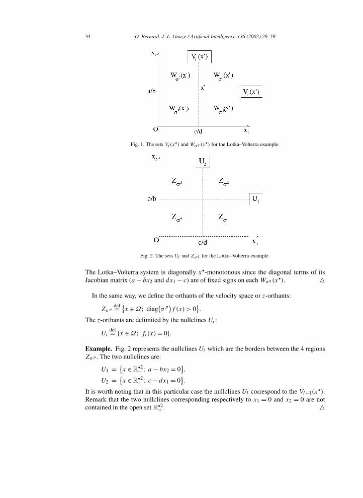
Fig. 1. The sets Vi(x) and Wσq (x) for the Lotka–Volterra example.
Fig. 2. The sets Ui and Zσq for the Lotka–Volterra example.
The Lotka–Volterra system is diagonally x-monotonous since the diagonal terms of itsJacobian matrix (a − bx2 and dx1 − c) are of fixed signs on each Wσ q (x
).
In the same way, we define the orthants of the velocity space or z-orthants:
Zσpdef=x ∈Ω; diag
(σp)f (x) > 0
.
The z-orthants are delimited by the nullclines Ui :
Uidef= x ∈Ω; fi(x)= 0.
Example. Fig. 2 represents the nullclines Ui which are the borders between the 4 regionsZσp . The two nullclines are:
U1 =x ∈ R
2+ ; a − bx2 = 0
,
U2 =x ∈ R
2+ ; c− dx1 = 0
.
It is worth noting that in this particular case the nullclines Ui correspond to the Vi+1(x).
Remark that the two nullclines corresponding respectively to x1 = 0 and x2 = 0 are notcontained in the open set R
2+ .
O. Bernard, J.-L. Gouzé / Artificial Intelligence 136 (2002) 29–59 35
We consider also the following sets that are unions of sets previously defined:
• The union set of hyperplanes associated with x: V (x) def=⋃n
i=1 Vi(x).
• The union set of nullclines: U def=⋃n
i=1Ui .
3. The set of possible qualitative events
In this section we will consider a monotonous (i.e., with monotonous interactions) loopstructured system (Σ) and we will suppose that there exists an equilibrium point x ∈Ω
for which (Σ) is diagonally x-monotonous. We will then determine the set of orthants ofthe velocity space Zσp compatible with a given orthantWσ q (x
) of the x-deviation space.In other words the question is to determine all the possible signs of f (x) for x in a givenx-orthant, i.e., the following set of signs:
Fq def
=sign
(f (x)
), x ∈Wσ q (x
) \U. (4)
In QSIM terminology [20], the goal of this section is to provide the constraints thatdetermine the possible qualitative states of the system.
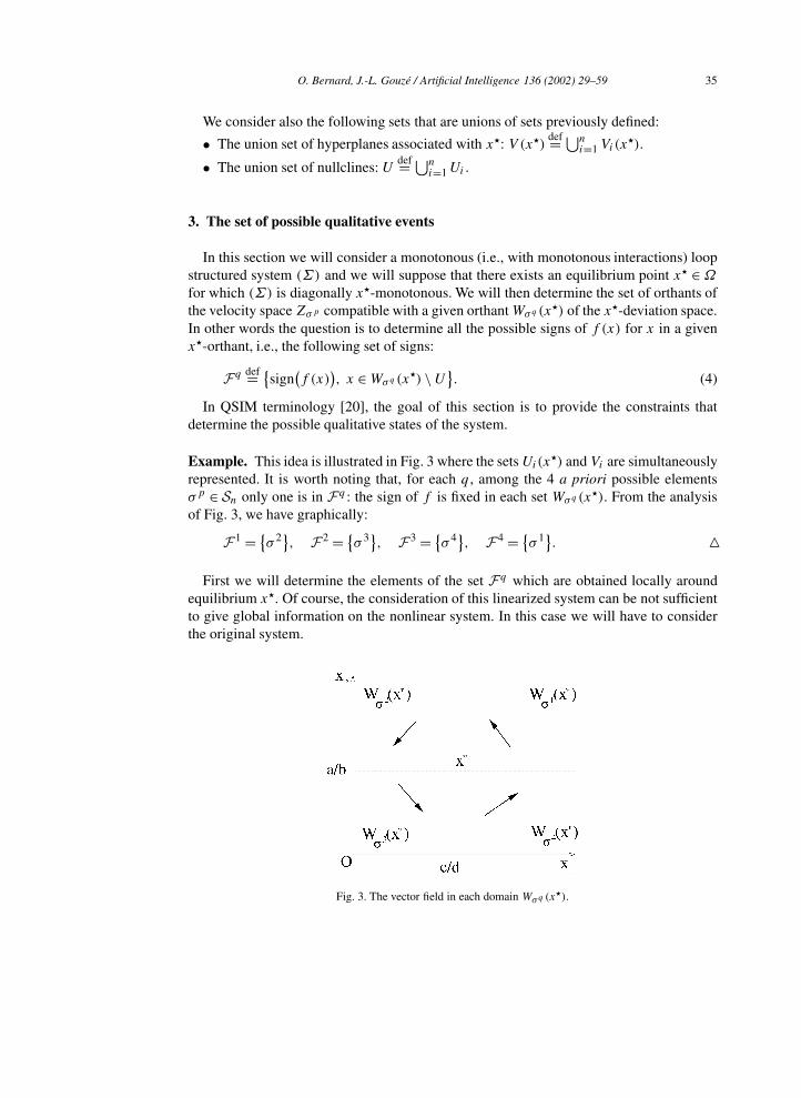
Example. This idea is illustrated in Fig. 3 where the sets Ui(x) and Vi are simultaneouslyrepresented. It is worth noting that, for each q , among the 4 a priori possible elementsσp ∈ Sn only one is in Fq : the sign of f is fixed in each set Wσ q (x
). From the analysisof Fig. 3, we have graphically:
F1 =
σ 2, F
2 =σ 3, F
3 =σ 4, F
4 =σ 1.
First we will determine the elements of the set Fq which are obtained locally aroundequilibrium x. Of course, the consideration of this linearized system can be not sufficientto give global information on the nonlinear system. In this case we will have to considerthe original system.
Fig. 3. The vector field in each domain Wσq (x).
36 O. Bernard, J.-L. Gouzé / Artificial Intelligence 136 (2002) 29–59
3.1. Linear approach
As a first step, we will determine this set for the linearized of (Σ) around the point x,which is:
$x =Df (x)$x, (5)
where Df (x) denotes the Jacobian matrix at point x , and $xdef= x − x. Note that
diag(σ q)$x is a positive vector for x ∈ Wσ q (x). Of course, as for the nonlinear case,
we will exclude the nullclines of the linear system (linearized of a Ui ).
We will consider the matrix Mq def= Df (x)diag(σ q), whose elements are denoted mq
kl
and whose signs are sqkl = sign(mqkl).
Example. At the point x, the Jacobian matrix is:
Df (x)=
(0 −bc/d
ad/b 0
).
We have then the signs of the four matrices Mq :
sign(M
1) =
(0 −11 0
), sign
(M
2)=
(0 −1
−1 0
),
sign(M
3) =
(0 1
−1 0
), sign
(M
4)=
(0 11 0
).
The problem of determining the possible signs forDf (x)$x when x ∈Wσ q (x) is then
equivalent to the determination of the set
Lq def
=sign
(M
q ξ), ξ > 0, (ξ + x) ∈Ω
. (6)
Of course we have Lq ⊂ Fq : the sign patterns allowed close to x are included in theset of all possible sign patterns for the original nonlinear system.
We will determine the set Lq , using two complementary lemma (remember that the sqkltake their values in −1,0,1).
Lemma 1. Consider the linearized of a diagonally x-monotonous loop structured system(Σ), at point x ∈ Ω . For a given σ q , if there exists an index k such that one of the twoconditions is satisfied:
(1) sqk,k = 0,
(2) sq
k,k = sq
k,k+1,then
Lq =
lq = t(lq1 , . . . , l
qn
); l
qj ∈
sqj,j ⊕ s
q
j,j+1. (7)
The table of the operator ⊕ (“generic qualitative sum”) is given in Table 1.
Proof. Cf. Appendix A.

O. Bernard, J.-L. Gouzé / Artificial Intelligence 136 (2002) 29–59 37
Table 1Table of rules for the (com-mutative) qualitative sum ⊕
1 ⊕ 1 1
−1 ⊕ 1 −1,1
−1 ⊕ −1 −1
−1 ⊕ 0 −1
1 ⊕ 0 1
0 ⊕ 0 0
Lemma 1 states that, under the given conditions, all the signs a priori admissible areobtained. The following lemma covers the remaining cases, and it turns out that things area bit more complicated:
Lemma 2. Consider the linearized of a diagonally x-monotonous loop structured system(Σ), with x ∈Ω .
If for every index k: sqk,k = −sq
k,k+1, then
Lq = Sn − C
q , (8)
where the set Cq is obtained as follows from Dq def= t(s
q
1,1, sq
2,2, . . . , sqn,n):
• if det[Df (x)]< 0,
Cq =
n∏
j=1
σqj s
qj,j D
q
,
• if det[Df (x)] = 0,
Cq =
−
n∏
j=1
σqj s
qj,j D
q ,
n∏
j=1
σqj s
qj,j D
q
,
• if det[Df (x)]> 0,
Cq =
−
n∏
j=1
σqj s
qj,j D
q
.
Proof. Cf. Appendix B.
In this particular case one has to remove from the set of a priori admissible signs (whichis Sn here) the particular element Cq .
Example. Here we are in the case 1 of Lemma 1 where there exists an index k such thatsqk,k = 0 (k = 1 or k = 2). Hence:
L1 =
σ 2, L
2 =σ 3, L
3 =σ 4, L
4 =σ 1.
38 O. Bernard, J.-L. Gouzé / Artificial Intelligence 136 (2002) 29–59
3.2. Global approach
In order to determine the set of possible signs for f (x), we will rewrite the system (Σ)
into another form. Using the fact that Lq ⊂ Fq , we will determine the various cases forwhich this inclusion is strict.
Lemma 3. If x is an equilibrium point, the system (Σ) can be rewritten
$x =A(x,x).$x.
If (Σ) has monotonous interactions, then matrix A(x,x) has the same off-diagonal signsas the Jacobian matrix Df (x) of (Σ). If moreover (Σ) is diagonally x-monotonous,the diagonal terms of A(x,x) are of fixed signs in the various Wσ q (x
). The diagonalelements of A(x,x) have the same sign as those of Df (x) (except for the elements ofDf (x) that are zero).
Proof. This is an application of the generalized first order Taylor formula [30]:
f (x)= f (x)+
[ 1∫
0
Df(αx + (1 − α)x
)dα
](x − x)
so that
A(x,x)=
1∫
0
Df(αx + (1 − α)x
)dα,
where the Jacobian matrix Df is of fixed sign on Ω . The results follow easily from theconvexity of Ω [6].
Example. We have for the Lotka–Volterra system:
A(x,x)=
(a − b/2(x2 + x2) −b/2(x1 + x1)
d/2(x2 + x2) d/2(x1 + x1)− c
). (9)
We will use the same notations for A(x,x) as for Df (x), i.e., we will denoteMq(x)=A(x,x)diag(σ q), and tqkl the (fixed) sign of its elements mq
kl(x).We first consider the simple case where the diagonal elements of the Jacobian matrix are
nonzero (and therefore matrix A(x,x) and Df (x) are of the same sign (cf. Lemma 3)).In this case the simple framework of Lemma 1 is satisfied:
Lemma 4. Consider a diagonally x-monotonous loop system (Σ) where x is anequilibrium point. If the following two conditions hold in Wσ q (x
):(1) ∀k, t
qk,k = s
qk,k = 0,
(2) ∃k, tq
k,k = tq
k,k+1,then we have Fq = Lq .
O. Bernard, J.-L. Gouzé / Artificial Intelligence 136 (2002) 29–59 39
Proof. It is straightforward that Fq ⊂ lq; lqj ∈ t
qj,j ⊕ t
qj,j+1, for the same reasons as in
the local case, when considering zk =mqk,k(x)ξk +m
q
k,k+1(x)ξk+1 (see Appendix A for thenotations).
But Lq = lq; lqj ∈ s
qj,j ⊕ s
q
j,j+1t ⊂ Fq , and because the sq equal the tq we haveFq = Lq .
Remark 1. If sqk,k = 0 and tqk,k = 0, no conclusion can be drawn in the general case on thepossible signs of the kth component zk and one has to consider the analytical formulationof the model. Consider for example the following differential system defined on R
2:x1 = x2 − x2
1 ,
x2 = x1 − x22 .
(10)
For the equilibrium point x = t(0,0), the Jacobian matrix has the following signs:(
0 +
+ 0
)(11)
so that for x in R2+ , Lq = σ 1. Nevertheless the matrix A(x,x) has the following signs:
(− +
+ −
)(12)
and it is clear from (10) that Fq = S2.
Example. The above remark applies to the Lotka–Volterra system. Fig. 3 showsnevertheless that the nonlinear part does not provide more qualitative possibilities thanthe linear case: Fq = Lq .
We will now consider the other case corresponding to Lemma 2.
Lemma 5. Consider a diagonally x-monotonous loop system (Σ) where x is anequilibrium point. Suppose that for all k we have tqk,k = −t
q
k,k+1.If det(A(x, x)) cancels and changes its sign on Wσ q (x
), then the set Fq covers all thepossible orthants:
Fq = Sn (13)
if this is not the case, then
Fq = Sn − C
q , (14)
where the set Cq is obtained as follows from Dq def= t(t
q
1,1, tq
2,2, . . . , tqn,n):
• if det[A(x†, x)]< 0,
Cq =
n∏
j=1
σqj s
qj,j D
q
,
• if det[A(x†, x)]> 0,
Cq =
−
n∏
j=1
σqj s
qj,j D
q
,
x† ∈Wσ q (x) being any point where the determinant of A(x†, x) does not cancel.
40 O. Bernard, J.-L. Gouzé / Artificial Intelligence 136 (2002) 29–59
Proof. We have Lq ⊂ Fq ⊂ Sn. From Lemma 8, we know that Lq corresponds to Sn
except one or two elements. The question is to know if these elements can neverthelessbe in Fq . To answer this question, the same reasoning can be made as for the proof ofLemma 8, considering now zk =m
qk,k(x)ξk +m
qk,k+1(x)ξk+1. This reasoning will give rise
to a constraint on the sign of the determinant of A(x,x).If the determinant can change its sign on Wσ q (x
), then Dq or −Dq is possible onWσ q (x
).
Remark. Let us remark that if there exists another equilibrium point x† ∈Wσ q (x), then
A(x†, x)(x† − x)= 0 and therefore
det(A(x†, x)
)= 0.
Then we are in the case of the above lemma.
3.3. Partition of the state space: possible regions
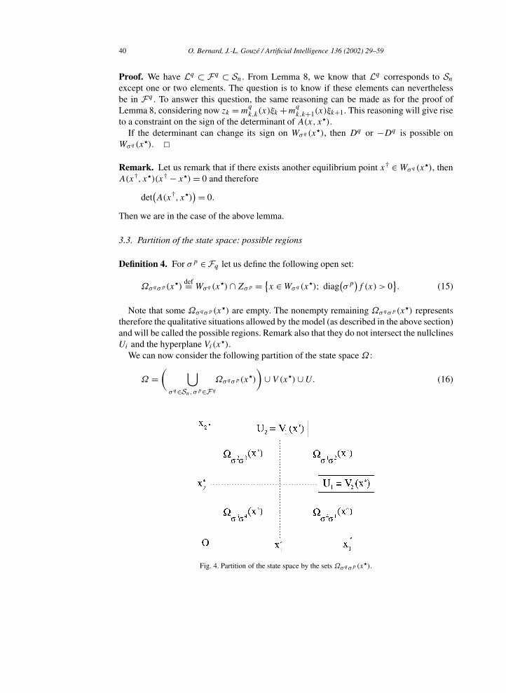
Definition 4. For σp ∈Fq let us define the following open set:
Ωσ qσp (x)
def= Wσ q (x
)∩Zσp =x ∈Wσ q (x
); diag(σp)f (x) > 0
. (15)
Note that some Ωσ qσp (x) are empty. The nonempty remaining Ωσ qσp (x
) representstherefore the qualitative situations allowed by the model (as described in the above section)and will be called the possible regions. Remark also that they do not intersect the nullclinesUi and the hyperplane Vi(x).
We can now consider the following partition of the state space Ω :
Ω =
( ⋃
σ q∈Sn, σp∈Fq
Ωσ qσp (x)
)∪ V (x)∪U. (16)
Fig. 4. Partition of the state space by the sets Ωσqσp (x).
O. Bernard, J.-L. Gouzé / Artificial Intelligence 136 (2002) 29–59 41
Example. As a conclusion of the previous paragraph, we have seen that only the four setsΩσ 1σ 2(x),Ωσ 2σ 3(x),Ωσ 3σ 4(x) and Ωσ 4σ 1(x) were not empty. The state space Ω isnow partitioned according to Fig. 4.
4. The restricted phase space
We remove here from Ω some manifolds for which trajectories may have undesirablebehaviors (with respect to our goals): we show that this set of trajectories is of measurezero, under some technical assumptions. The final phase space will be named Ω . Thetechnical details that guarantee that the removed trajectories are of zero measure (andtherefore will not be observed) are presented in Appendix C.
Now we are able to define the open set Ω , which is Ω minus these sets of measure zero(in finite number) from the three properties presented in Appendix C (Properties C.2–C.4).In the particular case (let us call it case E) where the two surfacesUi and Vi−1(x
∗) coincideon an open set, we do not remove the corresponding set. From now on, everything will takeplace in this restricted space Ω . For a possible regionΩσ qσp (x
) (see Section 3), we definethe nonempty set:
Ωσ qσp (x)
def= Ωσ qσp (x
)∩ Ω
and the neighbors in Ω : two regions of the phase space are neighbors if they differ onlyby one sign (of a deviation or a velocity). It is to be remarked that we have suppressed (byrestricting Ω) the possibility of going from one region Ωσ qσp (x
) to another if they differby more than one sign (except in the last case E which is a bit degenerate, but will occur inthe example of Section 6).
Definition 5. Two domains Ωσ q1σp1 (x) and Ωσ q2σp2 (x
) are called:• strict U -neighbors if σ q1 = σ q2 , and there exists a unique k ∈ 1, . . . , n such thatσp1k = −σ
p2k ;
• strict V -neighbors if σp1 = σp2 , and there exists a unique k ∈ 1, . . . , n such thatσq1k = −σ
q2k .
Definition 6. In the case E, we say that Ωσ q1σp1 (x) and Ωσ q2σp2 (x
) are strict UV -neighbors if for all i = k, σ
p1i = σ
p2i , σ
q1i+1 = σ
q2i+1 and σp1
k = −σp2k , σ
q1k+1 = −σ
q2k+1.
Example. In dimension 2 none of the trajectories must be removed, therefore Ω = Ω .For the Lotka–Volterra system, the equilibrium hyperplanes Vi(x) are included in thenullclines Ui+1 (we are in case E) and therefore the sets Ωσ iσ i+1(x) and Ωσ i+1σ i+2(x)
are strict UV -neighbors.
5. Transition between the domains Ωσ qσp (x)
We can now consider the restricted space Ω partitioned in open domains Ωσ qσp (x).
We will then show that the transition between these domains obey some rules determinedby the extradiagonal terms of the Jacobian matrix.
42 O. Bernard, J.-L. Gouzé / Artificial Intelligence 136 (2002) 29–59
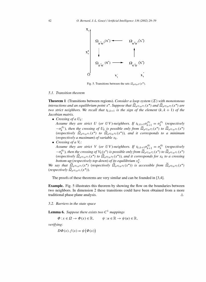
Fig. 5. Transitions between the sets Ωσqσp (x).
5.1. Transition theorem
Theorem 1 (Transitions between regions). Consider a loop system (Σ) with monotonousinteractions and an equilibrium point x. Suppose that Ωσ q1σp1 (x
) and Ωσ q2σp2 (x) are
two strict neighbors. We recall that tk,k+1 is the sign of the element (k, k + 1) of theJacobian matrix.
• Crossing of a Uk:Assume they are strict U (or UV )-neighbors. If tk,k+1σ
p1k+1 = σ
p1k (respectively
−σp1k ), then the crossing of Uk is possible only from Ωσ q2σp2 (x
) to Ωσ q1σp1 (x)
(respectively Ωσ q1σp1 (x) to Ωσ q2σp2 (x
)), and it corresponds to a minimum(respectively a maximum) of variable xk .
• Crossing of a Vi :Assume they are strict V (or UV )-neighbors. If tk,k+1σ
q1k+1 = σ
q1k (respectively
−σq1k ), then the crossing of Vk(x) is possible only from Ωσ q2σp2 (x
) to Ωσ q1σp1 (x)
(respectively Ωσ q1σp1 (x) to Ωσ q2σp2 (x
)), and it corresponds for xk to a crossingbottom-up (respectively top-down) of its equilibrium xk .
We say that Ωσ q1σp1 (x) (respectively Ωσ q2σp2 (x
)) is accessible from Ωσ q2σp2 (x)
(respectively Ωσ q1σp1 (x)).
The proofs of these theorems are very similar and can be founded in [3,4].
Example. Fig. 5 illustrates this theorem by showing the flow on the boundaries betweentwo neighbors. In dimension 2 these transitions could have been obtained from a moretraditional phase plane analysis.
5.2. Barriers in the state space
Lemma 6. Suppose there exists two C1 mappings
Φ :x ∈Ω →Φ(x) ∈ R, ψ :u ∈ R →ψ(u) ∈ R,
verifying:
DΦ(x).f (x)=ψ(Φ(x)
)
O. Bernard, J.-L. Gouzé / Artificial Intelligence 136 (2002) 29–59 43
then Rdef= x ∈Ω; ψ(Φ(x))= 0 separates Ω into positively invariant regions,
R− def
=x ∈Ω; ψ
(Φ(x)
)< 0
and R
+ def=x ∈Ω; ψ
(Φ(x)
)> 0
.
Proof. If we set u=Φ(x), u satisfies the first order scalar differential equation u=ψ(u).The zeros of ψ separate the space into invariant regions where ψ is always positive ornegative.
Corollary 1. If there exists a region of the state space Ωσ qσp (x) such that: Ωσ qσp (x
)∩
R− = ∅ (respectively Ωσ qσp (x) ∩ R+ = ∅), then any trajectory initiated in R−
(respectively in R+) will never reach the region Ωσ qσp (x).
Corollary 2. Any trajectory initiated in a region Ωσ q1σp1 (x) ⊂ R+ (respectively
Ωσ q1σp1 (x) ⊂ R−), will never reach the regions Ωσ q2σp2 (x
) ⊂ R− (respectivelyΩσ q2σp2 (x
)⊂R+).
Remarks.• Such a property is quite frequent, for example in biotechnological models, where u is
linked to mass conservation, and ψ is linear [1].• Because u verifies a scalar differential equation, the nonempty limit sets are the
equilibria; property P thus holds (cf. Appendix C).
5.3. Main theorem of behavior
The following theorem describes the behavior of the trajectories of a differentialsystem (Σ) with monotonous interactions, loop structured and diagonally-monotonous:the domain Ω , restricted to Ω (cf. Section 4) is partitioned into the possible regionsΩσ q1σp1 (x
) (Section 3); the possible transition rules between these regions (cf. Section 5)are given by Theorem 1.
Theorem 2 (Global qualitative behavior). Every trajectory of (Σ) in a domain Ωσ qσp (x)
either:• stays in Ωσ qσp (x
) and goes to infinity;• stays in Ωσ qσp (x
), and goes towards an equilibrium x† in the closure of Ωσ qσp (x);
• goes to one of the strict neighbors Ωσ q
′σp
′ (x) that are accessible.
Proof. Indeed, if a trajectory remains in a possible Ωσ qσp (x) (Section 3), then the xk are
of fixed sign, therefore the xk are monotonous. If they are bounded, they have to convergetowards an equilibrium in the closure of Ωσ qσp (x
) or to go towards an accessible neighbor(Section 5). Moreover, this neighbor must be a strict neighbor, because we have removedthe trajectories going to nonstrict neighbors (Section 4).
Remark 2. Note that the trajectories cannot become unbounded in a domain Ωσ qσp (x)
where for all i , σ qi = −σpi , because that would mean that the state variables are decreasing

44 O. Bernard, J.-L. Gouzé / Artificial Intelligence 136 (2002) 29–59
above their equilibrium, or increasing under their equilibrium. If the state variables arepositive (as often in biological modeling), a necessary condition for unboundedness inΩσ qσp (x
) is that there exists i for which σ qi = σpi = 1.
Remark 3. The equilibrium x can be reached from a domain Ωσ qσp (x) if and only
if σpk = −σq
k for all k. If this condition is not fulfilled for some k, then variable xk isdecreasing under its equilibrium xk , or increasing above its equilibrium and can thereforenot converge.
Remark 4. A local linear study can also give interesting information on the possibility ofconvergence in a given region [4].
5.4. Graphical representation
We will represent each possible region Ωσ qσp (x) by a two column matrix of signs:
the first column stands for σ q , and the second for σp . For example, the region x ∈ Ω;
x1 > x1, x2 < x2, x3 > x3, x1 < 0, x2 < 0, x3 > 0 is represented by the matrix:(
+ −
− −
+ +
).
A possible transition between two regions is represented by an oriented arrow betweenthese regions, as determined by the conclusions of Theorem 1. A letter on the arrow willindicate if the variable xk admits a minimum (mk), a maximum (Mk), if it crosses itsequilibrium xk top-down (tk) or bottom-up (Tk). The set of all Ωσ qσp (x
) related by thearrows reflecting the transition rules of Theorem 1 is called the basic mixed transitiongraph. The nodes for which it is possible to converge to equilibrium (cf. Remark 3) will becalled equilibrium nodes.
Our main theorem has now a “graphical version” (cf. the detailed example below andFigs. 8 and 9). For the sake of simplicity, we will restrict ourselves to the case where allthe trajectories are bounded. We obtain then (cf. Figs. 8 and 9):
Theorem 3 (Graphical version of the global qualitative theorem). On each nonequilibriumnode, the trajectories follow an arrow of the graph and go towards an accessible node. Oneach equilibrium node, the trajectories either stay in the node and converge to equilibrium,or go towards an accessible node.
Example. Now the qualitative behavior of the prey-predator system can be representedby a transition graph (Fig. 6). Fig. 5 illustrates this theorem by showing the flow on theboundaries between two neighbors.
5.5. Asymptotic behavior
Some theorems (admitting a simple interpretation in terms of the graph) on the behaviorof loop structured systems with monotonous interactions have already been given [4]. We

O. Bernard, J.-L. Gouzé / Artificial Intelligence 136 (2002) 29–59 45
Fig. 6. Transition graph for the Lotka–Volterra system. Each node of the graph represents a qualitative feature:the first column deals with the sign of the deviation from the equilibrium point, and the second column representsthe trend of the variable. mi (respectively Mi ) stands for a minimum (respectively a maximum) of xi , and ti(respectively Tk ) represents a crossing of its equilibrium value top-down (respectively bottom-up).
will just give the following lemma, derived from considerations of both deviation from areference point and trends of the variables.
Lemma 7. If, in the transition graph of a system Σ , there is no cycle containing anextremum of variable xk , then for almost every trajectories, xk either goes towards anequilibrium in the closure of Ω or to infinity.
Corollary 3. If there is no cycle in the transition graph of a system Σ , almost all thetrajectories go towards an equilibrium in the closure of Ω or diverge.
In other words, it means that there is no periodic or recurrent behavior, nor chaos orother complex behavior.
6. Application: qualitative behavior of a general class of cell growth models
6.1. The class of models
To illustrate the qualitative analysis of loop structured systems we will consider anontrivial application: the growth of phytoplankton in the oceans. We will consider aclass of models used in oceanography to estimate the amount of carbon uptaken by thephytoplankton during the photosynthesis process. These models describe the behavior ofphytoplanktonic biomass (x2) growing on a substrate (x1).
In the laboratory, the algal growth process in a continuous reactor (chemostat), fordimensionless variables (for a nonzero nutrient supply) can be described by the followingsystem:
(ΣPGM)
x1 = 1 − x1 − ρ(x1)x2,
x2 = (µ(x3)− 1)x2,
x3 = ρ(x1)−µ(x3)x3.
(17)
46 O. Bernard, J.-L. Gouzé / Artificial Intelligence 136 (2002) 29–59
The variable x3 is the cell quota, i.e., the quantity of intracellular nutrient per biomassunit. The functions ρ and µ respectively represent the absorption rate of the substrate andthe growth rate.
The validation of this class of models by comparison with experimental data is given in[6]. For more mathematical details on the models in the chemostat see [26].
Among the models (ΣPGM), the Droop model [8,12] is largely used in the biologicalfield. For this particular model we have:
ρ(x1)= a1x1
a2 + x1; µ(x3)= a3
(1 −
a4
x3
).
The functions used for ρ and µ are only conjectures and are not justified by a propervalidation for transient conditions. In the following we keep a more general framework andwe do only qualitative hypotheses, so that the analysis can be applied to any reasonable ρand µ.
Hypotheses. Some hypotheses, corroborated by the experiments, are generally made bythe biologists in order to represent growth of phytoplankton [22]: in the considered physicaldomain, Ω = x ∈ R
3+ ;x1 > 0, x2 > 0, x3 > 0:
(H1) The absorption rate ρ is a nonnegative bounded function of x1. It is strictlyincreasing and verifies ρ(0)= 0.
(H2) The growth rate µ is a nonnegative strictly increasing function of x3.(H3) An equilibrium exists in the open domain Ω .The class of models (ΣPGM) verifying hypothesis (H1)–(H2)–(H3) is called the class of
Phytoplanktonic Growth Models (PGMs). It can easily be verified that the Droop model isin this class.
6.2. The PGMs: a nontrivial loop structured class of systems with monotonousinteractions
Property 1. The PGMs are loop structured models with monotonous interactions in Ω .
Proof. The Jacobian matrix has the following signs on Ω :(
−1 −1 00 t22(x) +1
+1 0 −1
)(18)
with
t22(x)= sign(x2)= sign(µ(x3)− 1
). (19)
Property 2. The PGMs have two equilibria:• x ∈Ω :
x3 = µ−1(1); x1 = ρ−1(µ−1(1)); x2 =
1 − ρ−1(µ−1(1))µ−1(1)
.

O. Bernard, J.-L. Gouzé / Artificial Intelligence 136 (2002) 29–59 47
• xb, an unstable equilibrium on the boundary of Ω :
xb2 = 0; xb1 = 1; xb3 unique solution of: µ(xb3)xb3 = ρ
(xb1).
Proof. In accordance with hypothesis (H3), we have x ∈ Ω , i.e., x2 > 0. Hypotheses(H1) and (H2) ensure the uniqueness of this equilibrium, because the applications µ−1 andρ−1 µ−1 are strictly increasing. Moreover, it is straightforward from a local study that xb
is unstable if x2 > 0.We will then consider the three hyperplanes Vi(x)= x ∈Ω; x = xi which separate
the space Ω into eight regions Wσ j (x).
Property 3. The PGMs are diagonally x-monotonous in the domain Ω .
Proof. It can be noticed that t22(x)= sign(x3 − x3), therefore in each domain Wσ q (x),
t22(x)= σq
3 is fixed. We therefore have sign(x2)= sign(x3 − x3)= σq
3 .We are therefore in the case E of Property C.4 (with V3(x
) ⊂ U2), it means thatsimultaneously when x2 reaches an extremum, x3 crosses its equilibrium x3 .
Property 4 (Mass conservation). If u= Φ(x) denotes the total nutrient concentration inthe chemostat:
udef= x1 + x2x3 (20)
u satisfies the following differential equation:
u= 1 − u. (21)
Property 5. The trajectories of the PGMs are bounded in the positively invariantdomain Ω .
Proof. The proof of Property 4 is straightforward from system (17). To show that Ω ispositively invariant one has to consider the field on the boundaries:
• From (H1), for every x on the face x1 = 0 we have: x1 = 1> 0.• For every x on the face x2 = 0 it holds: x2 = 0.• For every x on the face x3 = 0: x3 0.
Moreover, to prove the boundedness of the trajectories, we first use Property 4 to show thatu is bounded, i.e., x1 and the product x2x3 are bounded.
To show that x3 is bounded, we consider a real a large enough to ensure that the strictlyincreasing function µ(a)a becomes larger than the upper bound of ρ (cf. (H1)). It followsthat the field on every hyperplane x3 = b, where b a, verifies: x3 < 0.
The product x2x3 is bounded, so that x2 is also bounded (cf. [4] for details).
In the sequel, we will remove the set of trajectories initiated from the manifoldspresented in Table 2. Note that for a loop structured system with monotonous interaction indimension 3, it is impossible to cross simultaneously two sets Ui (see [4]). The same proofshows that it is also impossible to cross simultaneously two sets V3(x
). As a consequence,the following results hold on the restricted set Ω :
Ω =Ω \U1 ∩ V3(x
),U3 ∩ V2(x).
48 O. Bernard, J.-L. Gouzé / Artificial Intelligence 136 (2002) 29–59
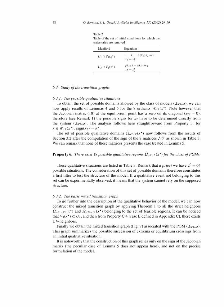
Table 2Table of the set of initial conditions for which thetrajectories are removed
Manifold Equations
U1 ∩ V3(x)
1 − x1 − ρ(x1)x2 = 0x3 = x3
U3 ∩ V2(x)
ρ(x1)=µ(x3)x3x2 = x2
6.3. Study of the transition graphs
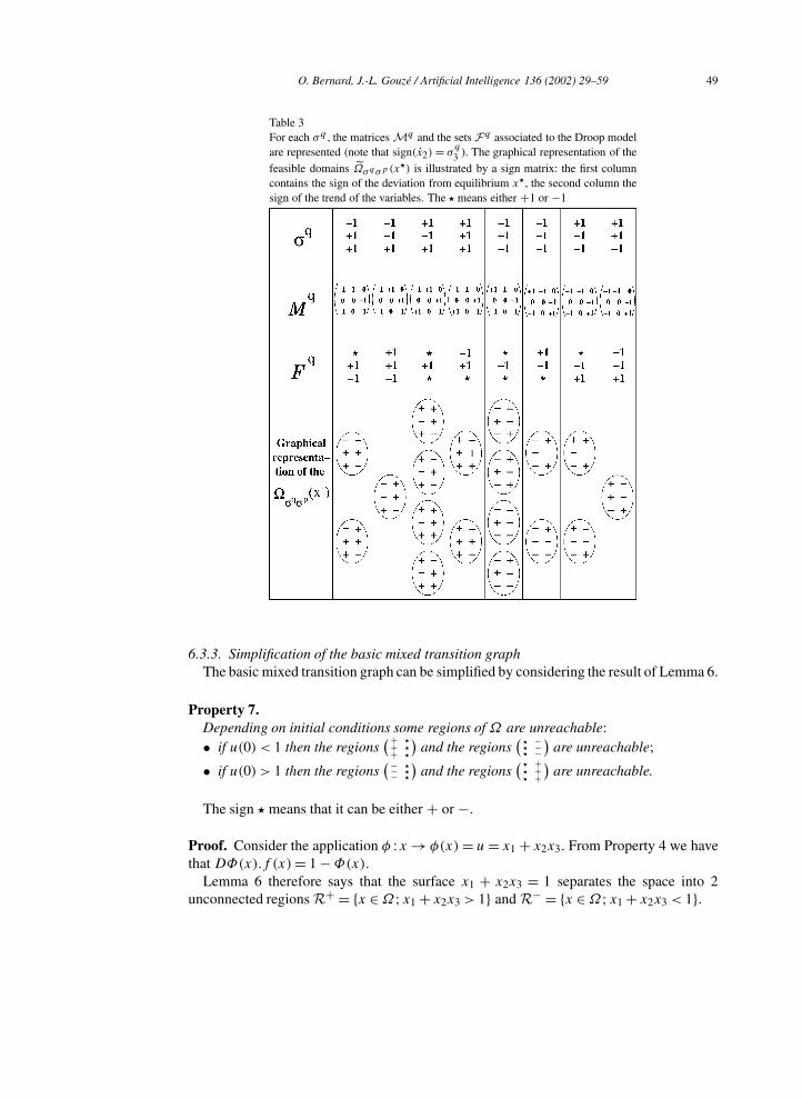
6.3.1. The possible qualitative situationsTo obtain the set of possible domains allowed by the class of models (ΣPGM), we can
now apply results of Lemmas 4 and 5 for the 8 orthants Wσ q (x). Note however that
the Jacobian matrix (18) at the equilibrium point has a zero on its diagonal (s22 = 0),therefore (see Remark 1) the possible signs for x2 have to be determined directly fromthe system (ΣPGM). The analysis follows here straightforward from Property 3: forx ∈Wσ q (x
), sign(x2)= σq3 .
The set of possible qualitative domains Ωσ qσp (x) now follows from the results of
Section 3.2 after the computation of the sign of the 8 matrices Mq as shown in Table 3.We can remark that none of these matrices presents the case treated in Lemma 5.
Property 6. There exist 18 possible qualitative regions Ωσ qσp (x) for the class of PGMs.
These qualitative situations are listed in Table 3. Remark that a priori we have 26 = 64possible situations. The consideration of this set of possible domains therefore constitutesa first filter to test the structure of the model. If a qualitative event not belonging to thisset can be experimentally observed, it means that the system cannot rely on the supposedstructure.
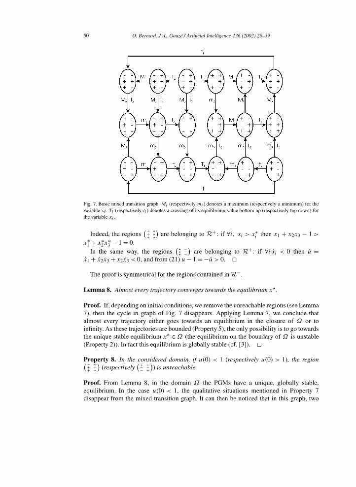
6.3.2. The basic mixed transition graphTo go further into the description of the qualitative behavior of the model, we can now
construct the mixed transition graph by applying Theorem 1 to all the strict neighborsΩσ q1σp1 (x
) and Ωσ q2σp2 (x) belonging to the set of feasible regions. It can be noticed
that V3(x)⊂U2, and then from Property C.4 (case E defined in Appendix C), there exists
UV-neighbors.Finally we obtain the mixed transition graph (Fig. 7) associated with the PGM (ΣPGM).
This graph summarizes the possible succession of extrema or equilibrium crossings froman initial qualitative situation.
It is noteworthy that the construction of this graph relies only on the sign of the Jacobianmatrix (the peculiar case of Lemma 5 does not appear here), and not on the preciseformulation of the model.
O. Bernard, J.-L. Gouzé / Artificial Intelligence 136 (2002) 29–59 49
Table 3For each σ q , the matrices Mq and the sets Fq associated to the Droop modelare represented (note that sign(x2)= σ
q3 ). The graphical representation of the
feasible domains Ωσqσp (x) is illustrated by a sign matrix: the first column
contains the sign of the deviation from equilibrium x , the second column thesign of the trend of the variables. The means either +1 or −1
6.3.3. Simplification of the basic mixed transition graphThe basic mixed transition graph can be simplified by considering the result of Lemma 6.
Property 7.Depending on initial conditions some regions of Ω are unreachable:• if u(0) < 1 then the regions
(+ + +
)and the regions
( − − −
)are unreachable;
• if u(0) > 1 then the regions(
− − −
)and the regions
( + + +
)are unreachable.
The sign means that it can be either + or −.
Proof. Consider the application φ :x → φ(x)= u= x1 + x2x3. From Property 4 we havethat DΦ(x).f (x)= 1 −Φ(x).
Lemma 6 therefore says that the surface x1 + x2x3 = 1 separates the space into 2unconnected regions R+ = x ∈Ω;x1 + x2x3 > 1 and R− = x ∈Ω;x1 + x2x3 < 1.
50 O. Bernard, J.-L. Gouzé / Artificial Intelligence 136 (2002) 29–59
Fig. 7. Basic mixed transition graph. Mi (respectively mi ) denotes a maximum (respectively a minimum) for thevariable xi . Ti (respectively ti ) denotes a crossing of its equilibrium value bottom up (respectively top down) forthe variable xi .
Indeed, the regions(+
+ +
)are belonging to R+: if ∀i, xi > x∗
i then x1 + x2x3 − 1 >x∗
1 + x∗2x
∗3 − 1 = 0.
In the same way, the regions( − − −
)are belonging to R+: if ∀i xi < 0 then u =
x1 + x2x3 + x2x3 < 0, and from (21) u− 1 = −u > 0.
The proof is symmetrical for the regions contained in R−.
Lemma 8. Almost every trajectory converges towards the equilibrium x.
Proof. If, depending on initial conditions, we remove the unreachable regions (see Lemma7), then the cycle in graph of Fig. 7 disappears. Applying Lemma 7, we conclude thatalmost every trajectory either goes towards an equilibrium in the closure of Ω or toinfinity. As these trajectories are bounded (Property 5), the only possibility is to go towardsthe unique stable equilibrium x∗ ∈ Ω (the equilibrium on the boundary of Ω is unstable(Property 2)). In fact this equilibrium is globally stable (cf. [3]).
Property 8. In the considered domain, if u(0) < 1 (respectively u(0) > 1), the region(− −+ ++ −
)(respectively
(+ +− −− +
)) is unreachable.
Proof. From Lemma 8, in the domain Ω the PGMs have a unique, globally stable,equilibrium. In the case u(0) < 1, the qualitative situations mentioned in Property 7disappear from the mixed transition graph. It can then be noticed that in this graph, two
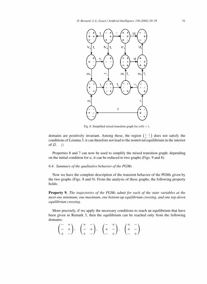
O. Bernard, J.-L. Gouzé / Artificial Intelligence 136 (2002) 29–59 51
Fig. 8. Simplified mixed transition graph for u(0) < 1.
domains are positively invariant. Among these, the region(− −
+ ++ −
)does not satisfy the
conditions of Lemma 3; it can therefore not lead to the nontrivial equilibrium in the interiorof Ω .
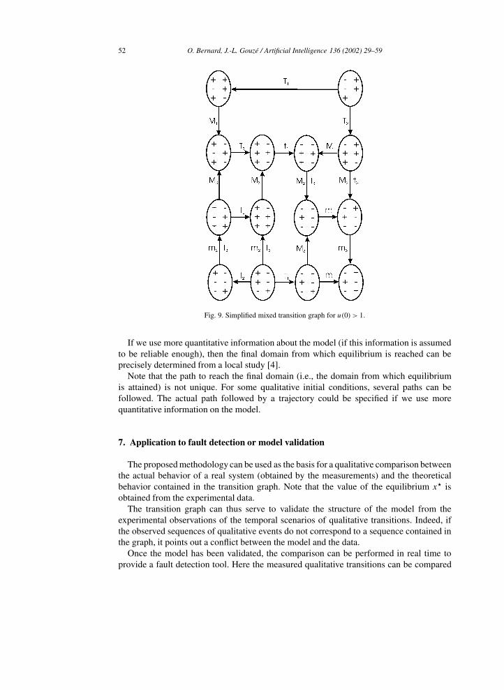
Properties 8 and 7 can now be used to simplify the mixed transition graph: dependingon the initial condition for u, it can be reduced to two graphs (Figs. 9 and 8).
6.4. Summary of the qualitative behavior of the PGMs
Now we have the complete description of the transient behavior of the PGMs given bythe two graphs (Figs. 8 and 9). From the analysis of these graphs, the following propertyholds:
Property 9. The trajectories of the PGMs admit for each of the state variables at themost one minimum, one maximum, one bottom-up equilibrium crossing, and one top-downequilibrium crossing.
More precisely, if we apply the necessary conditions to reach an equilibrium that havebeen given in Remark 3, then the equilibrium can be reached only from the followingdomains:
(− +
− +
+ −
),
(+ −
− +
+ −
),
(− +
+ −
− +
),
(+ −
+ −
− +
).
52 O. Bernard, J.-L. Gouzé / Artificial Intelligence 136 (2002) 29–59
Fig. 9. Simplified mixed transition graph for u(0) > 1.
If we use more quantitative information about the model (if this information is assumedto be reliable enough), then the final domain from which equilibrium is reached can beprecisely determined from a local study [4].
Note that the path to reach the final domain (i.e., the domain from which equilibriumis attained) is not unique. For some qualitative initial conditions, several paths can befollowed. The actual path followed by a trajectory could be specified if we use morequantitative information on the model.
7. Application to fault detection or model validation
The proposed methodology can be used as the basis for a qualitative comparison betweenthe actual behavior of a real system (obtained by the measurements) and the theoreticalbehavior contained in the transition graph. Note that the value of the equilibrium x isobtained from the experimental data.
The transition graph can thus serve to validate the structure of the model from theexperimental observations of the temporal scenarios of qualitative transitions. Indeed, ifthe observed sequences of qualitative events do not correspond to a sequence contained inthe graph, it points out a conflict between the model and the data.
Once the model has been validated, the comparison can be performed in real time toprovide a fault detection tool. Here the measured qualitative transitions can be compared

O. Bernard, J.-L. Gouzé / Artificial Intelligence 136 (2002) 29–59 53
to the transition graph [13,14]. If the transitions does not correspond to any path of thegraph, this means that the system behaves differently than the model which represents thestandard working mode. A mismatch between the observations and the graph will thencorrespond to a qualitative change (failure) in the process.
For both objectives (validation or fault detection), the transition graph will give us a setof criteria to diagnosis the origin of the fault (in the model for validation or in the systemfor fault detection). The diagnosis will be deduced from the localization of the constraintcontained in the graph that is violated. The reason for the conflict between the actual andthe theoretical behavior can be of two main types (we assume here that only one faulthappens at the same time):
• A transition for xi does not respect the direction of an arrow. This means that themodeling of variable xi is not consistent with the data. More precisely, it can resultfrom a sign change in the extradiagonal term of the Jacobian matrix associated withthis arrow (xi): the interaction between xi and xi+1 has changed. It can mean, e.g., thatvariable xi+1 is inhibiting xi instead of enhancing it. It can also be the consequenceof an interaction with another variable [7]. In this case, the loop structure is affected.A more detailed discussion of the use of the transition graphs to validate the structureof a model can be found in [4].
• An observed transition occurs towards a qualitative feature that does not exist in thegraph. If the transition was compatible with the transition rules imposed by the extra-diagonal terms of the Jacobian matrix, this may indicate that the topology of the spaceas induced by the partition of the Ωσ qσp (x
) is wrong. This points out a change in thesign of a diagonal term of the Jacobian matrix. It remains to find out which variableis affected by such a change. This can be done by exploring the effect of a change ineach of the signs of the diagonal elements on the possible regions Ωσ qσp .
The noise in the data can make the comparison—even on a qualitative basis—difficult.We have proved in [6] that the constraints dealing with the trends of the variables stillhold after removing noise with a simple moving average filter. This approach has beenapplied to analyze the response of a population of phytoplankton to a periodic input ofnutrient [6]. Although is was based only on the simple diagnosis obtained with trendsof the state, it revealed a qualitative change in the behavior of the population for highfrequency of nutrient supply: it seems that the cell division synchronizes on the nitrogensource.
Finally, the presented methodology can also be used in the context of model identifica-tion with an inverse problem perspective. How to find the model structure from a set ofdata? If there is a large number of available experiments which contain a sufficient amountof qualitative information (qualitative transitions), one can report these observations in agraph and observe the transitions that are always performed in the same way, and the qual-itative domains that are reached. This should lead to the identification of an experimentaltransition graph. The next step will then consist in finding a model structure that generatesthe observed graph. If the system has a loop structure (or a structure close to this idealcase), this will be straightforward from the proposed analysis. The important point is thatthis analysis is independent of the parameter values, as a consequence it only provides themodel structure. Quantitative modeling steps are then necessary to get a complete model-ing.
54 O. Bernard, J.-L. Gouzé / Artificial Intelligence 136 (2002) 29–59
This can find important applications, e.g., in the field of genomics, where data on thetemporal evolution of gene expression is available. This method could help to clarifythe interactions between the genes in the framework of the so called reverse engineeringapproach [10].
Of course, a computer implementation of the method will be necessary when the systemcomplexity will be too high. The complexity can both be due to an increase in thestate variables, or to additional interactions between the variables which make the modeldiffer from the loop structure. The implementation of the methods will then consist inautomatically generating a graph from the model structure and supporting the comparisonbetween the graph and the available experiments. Finally, for the reverse engineeringpurpose, it will allow to automatically identify a graph and generate possible modelstructures from the data analysis.
8. Conclusion
For the studied class of systems we have obtained a global qualitative description ofthe transient behavior as well as of the asymptotic behavior. We want to stress the factthat these results are global (i.e., they do not result from local linear considerations). Itis noteworthy that the qualitative behavior of these systems results only from the signsof the Jacobian (if we exclude the particular case for which the sign of the determinantmust be known). Therefore, this analysis is particularly well adapted to the biologicalcontext, where the only sure a priori knowledge of the process is the sign of the interactionsbetween variables.
In the analysis we have removed the trajectories for which two qualitative events appearat the same time (except for the case E defined in Appendix C). These trajectories are ofzero measure and thus they will never be observed in the real system. This simplifies theanalysis and differs from most of the qualitative studies where these special cases are notremoved.
Finally, let us stress that the hypothesis on the loop structure of the model is quite strong.In fact, our methodology can be applied (for a system with monotonous interactions)even if the system has not exactly a loop structure [3,5,7]. It is easy to see that sometransitions between two regions will be permitted in the two directions, allowing a morecomplex behavior. However, for the transitions being allowed in only one way, we arestill able to compare the model and the data. Moreover, it can happen that some regionsare still invariant (for example, if the Jacobian matrix has positive signs outside the maindiagonal, the region with positive signs is invariant). In this case it is possible to deriveinteresting results for such more general systems. Much work remains to be done in thisdirection.
Acknowledgements
We warmly thank Hidde de Jong (INRIA, Helix) for his constructive comments andsuggestions.
O. Bernard, J.-L. Gouzé / Artificial Intelligence 136 (2002) 29–59 55
Appendix A. Proof of Lemma 1
If σ ∈Lq , then there exists ξ ∈Ω+ such that: σ = sign(Mq ξ). If we denote z=Mq ξ ,we have:
zj =mq
j,j ξj +mq
j,j+1ξj+1.
While ξj and ξj+1 are positive, the possible signs σj for zj are in the set sqj,j , sqj,j+1
(remember that the sets zj = 0 have been removed).It follows that Lq ⊂Aq , where Aq is the set of a priori possible signs:
Aq def
=lq; l
q
j ∈sq
j,j ⊕ sq
j,j+1.
We will show that all the elements of Aq have a preimage by sign(Mqξ).If condition (1) or (2) is fulfilled for k, sign(zk)= s
q
k,k+1 = sq
k,k+1 ⊕ sq
k,k . We will fix ξkto an arbitrary positive value.
If we consider zk−1 =mq
k−1,k−1ξk−1 +mq
k−1,kξk , there exists two possibilities:(i) One of the two conditions is fulfilled: sqk−1,k−1 = 0 or sqk−1,k−1 = s
q
k−1,k . For anyξk−1 > 0, we have:
sign(zk−1)= sq
k−1,k = sq
k−1,k ⊕ sq
k−1,k−1.
(ii) In the other case, sqk−1,k−1 = −sq
k−1,k , and we choose:
ξk−1 = −εmq
k−1,k
mq
k−1,k−1ξk with ε ∈
12,
32
.
Then zk−1 = (1 − ε)mq
k−1,kξk . If we take ε = 12 we have sign(zk−1)= s
q
k−1,k , if wetake ε = 3
2 we obtain sign(zk−1)= −sq
k−1,k = sq
k−1,k−1.The same reasoning can be applied to zk−2, zk−3, . . . , z1, zn, . . . , zk+1, hence ξk−2, . . . ,
ξk+1 can be chosen such that the result follows.
Appendix B. Proof of Lemma 2
We will show that among the set Aq = Sn corresponding to the set of a priori possiblesigns for z (see argue given in the proof of Lemma 1), one single element is not inImsign(Mqξ).
(1) We will first assume that Dq = t(sq
1,1, sq
2,2, . . . , sqn,n)= σ 1, i.e., for every k: sqk,k = 1.
The other cases are symmetrical and they will be detailed at the end of the proof.We first show that it is possible to find ξ ∈ Ω+ such that there exists k for whichzkzk+1 < 0 (zk is defined in Appendix A). For the sake of clarity, we will first findsuch ξ ensuring z1 < 0 and zn > 0. For a fixed ξ2 > 0, it is possible to find ξ3 > 0such that z2 is of desired sign (cf. proof of preceding lemma). In the same wayξ4 > 0 to ξn > 0 can be chosen to obtain an arbitrary (and fixed) sign for z3 to zn−1 .
56 O. Bernard, J.-L. Gouzé / Artificial Intelligence 136 (2002) 29–59
Now we have to choose a ξ1 > 0 such that z1 < 0 and zn > 0. This is possible if wetake:
ξ1 <min(
−mq1,2
mq
1,1ξ2,−
mqn,n
mq
n,1ξn
).
This result can clearly be extended to all the situations where there exists an indexk such that zkzk+1 < 0.Let us prove that to find ξ such that z is positive, it is necessary to have det(Mq) > 0.Indeed, to have zp > 0 for every p, there must exists a positive ξ such that thefollowing conditions hold for every p:
ξp+1 <mqp,p
−mqp,p+1
ξp (B.1)
it follows that:
ξn <
n−1∏
j=1
mqj,j
−mqj,j+1
ξ1 <
n∏
j=1
mqj,j
−mqj,j+1
ξn. (B.2)
Condition (B.2) imposes:
λqdef=
n∏
j=1
mqj,j + (−1)n+1
n∏
j=1
mq
j,j+1 > 0. (B.3)
It is noteworthy that, for the loop structured system (Σ), λq is nothing but thedeterminant of matrix Mq :
λq = det(M
q)= det
(Df (x)
) n∏
j=1
σqj .
Reciprocally, let us show that if λq is positive, it is possible to find a positive ξ suchthat z is positive.First, we choose an arbitrary ξ1. We compute ξ2 to ξn by the following inductionformulae for 1 p n− 1:
ξp+1 = εmqp,p
−mqp,p+1
ξp (B.4)
with:
εdef=
(n∏
j=1
−mqj,j+1
mqj,j
)1/n
,
while λq is positive, it implies ε < 1, and thus condition (B.1) holds for 1 p
n − 1 implying zp > 0. We now have to prove that this gives also zn > 0. If wecompute ξn we get:
ξn = εn−1n−1∏
j=1
mq
j,j
−mq
j,j+1ξ1
O. Bernard, J.-L. Gouzé / Artificial Intelligence 136 (2002) 29–59 57
and then
mqn,n
−mq
n,1ξn =
ξ1
ε> ξ1
and therefore zn > 0.We have then found a positive ξ ensuring z > 0.
(2) The proof has now to be achieved by symmetry for a general Dq : the problematiccases correspond to sign(z) = Dq . The problem is then equivalent to findξ > 0 such that sign(diag(Dq )z) = σ 1, it consists therefore in considering matrixdiag(Dq )Mq , whose determinant is det[Df (x)]
∏nj=1 σ
q
j sq
j,j .
Appendix C. The set of trajectories that can be removed from Ω
C.1. Motivations
We want to remove a set of trajectories initiated from some (n− 2)-dimensional mani-foldM , typically the intersection between two isoclines. It is clear that, in finite time, such aset of trajectories is (n− 1)-dimensional, but the limit set (in positive time) can be, in some(rather intricate) case, of nonempty interior. This case is undesirable, because if we removethis set, it can be that we remove the trajectories that are experimentally observed. We willtherefore suppose that the differential system is such that the limit set of any manifold Mof dimension (n− 2) is of measure zero (property P). There are many cases where such aproperty is verified, and many ways to check it. Let us list some sufficient conditions:
• if the system admits a Lyapunov function for the equilibrium x∗, then it is globallystable. The limit set of any manifold is x∗ itself;
• if the system admits a function V (x) decreasing along the trajectories, then theLasalle’s theorem [19] gives us that the limit sets of any bounded trajectories arecontained into the set x; d
dt V (x)= 0. If this set is of measure zero (if it is containedin an (n− 1)-manifold for example), then the property is verified;
• if there exists an application h : Rn → Rp , with p < n of class C1, regular at every
point, such that
ddth(x)= g
(h(x)
)
along the trajectories of the system Σ , and if the limit sets of the new differentialsystem in R
p
(Σ1)
h= g(h)
verify property P, then the system Σ verifies property P (indeed, because of theregularity of h, the preimage of a set of measure zero is of measure zero). For example,if we know that the limit sets of Σ1 are a finite number of points (it is the case indimension one), then the property stands for Σ1, and therefore for Σ .For example, for biological, ecological or chemical models, it is often the casethat some mass balance or mass conservation relation holds, giving easily a scalardifferential equation; Property P is therefore verified.

58 O. Bernard, J.-L. Gouzé / Artificial Intelligence 136 (2002) 29–59
Now we examine each set of initial conditions of the trajectories we want to remove. Itis roughly the intersection between the Vi(x∗) and Uj , because there are two signs thatchange simultaneously. In all the following, we suppose that the above property P holds.
C.2. Remaining in a nullcline or in an equilibrium hyperplane
We recall first that it is not possible to stay on a nullcline.
Property C.1. A trajectory cannot remain in a Vi(x∗) set or in a Ui set, unless it is theequilibrium point x.
The proof is in [4]. The idea is to write that the manifold is invariant, and to differentiateenough times to obtain the result.
C.3. Intersecting nullclines and equilibrium hyperplanes
Property C.2. For loop structured systems with monotonous interactions, the set oftrajectories intersecting simultaneously two (different) Vi(x∗) is of measure zero.
Indeed, the intersection of the two hyperplanes xi = x∗i and xj = x∗
j is a (n − 2)-dimensional plane. Because of property P, the trajectories are of measure zero.
Property C.3. The set of trajectories intersecting simultaneously two (different) Ui is ofmeasure zero.
The intersection is defined by fi(x)= fj (x) = 0. The derivative of this application isof full rank two because the interactions are monotonous. Therefore the preimage of 0 is amanifold of dimension (n− 2), and property P applies.
Property C.4. For loop structured systems with monotonous interactions, the set oftrajectories intersecting simultaneously Ui and Vj (x∗) (j = i − 1) is of measure zero. Theset of trajectories intersecting simultaneouslyUi and Vi−1(x
∗) is of measure zero except inthe case (let us call it case E) where the system (Σ) is such that the two surfaces coincideon an open set.
In the first case, the intersection is defined by xi = x∗i , fj (xj , xj+1)= 0, and the same
reasoning as above applies. If j = i− 1, then the intersection x ∈Ω, fi−1(xi−1, xi )= 0
can be of dimension (n− 1): take for example the Lotka–Volterra system, the equilibriumhyperplane Vi(x) is included in the nullcline Ui+1.
References
[1] G. Bastin, D. Dochain, On-line Estimation and Adaptative Control of Bioreactors, Elsevier, Amsterdam,1990.

O. Bernard, J.-L. Gouzé / Artificial Intelligence 136 (2002) 29–59 59
[2] D. Berleant, B. Kuipers, Qualitative and quantitative simulation: Bridging the gap, Artificial Intelligence 95(1997) 215–255.
[3] O. Bernard, J.-L. Gouzé, Robust validation of uncertain models, in: A. Isidori (Ed.), Proc. 3rd EuropeanConference on Control, Rome, Italy, 1995, pp. 1261–1266.
[4] O. Bernard, J.-L. Gouzé, Transient behavior of biological loop models, with application to the Droop model,Math. Biosci. 127 (1) (1995) 19–43.
[5] O. Bernard, J.-L. Gouzé, Transient behavior of biological models as a tool of qualitative validation—Application to the Droop model and to a N-P-Z model, J. Biol. Syst. 4 (3) (1996) 303–314.
[6] O. Bernard, J.-L. Gouzé, Nonlinear qualitative signal processing for biological systems: Application to thealgal growth in bioreactors, Math. Biosci. 157 (1999) 357–372.
[7] O. Bernard, S. Souissi, Qualitative behavior of stage-structured populations: Application to structuralvalidation, J. Math. Biol. 37 (1998) 291–308.
[8] D.E. Burmaster, The unsteady continuous culture of phosphate-limited Monochrysis lutheri Droop:Experimental and theoretical analysis, J. Exp. Mar. Biol. Ecol. 39 (2) (1979) 167–186.
[9] H. Caswell, Matrix Population Models, Sinauer Associates Publishers, 1989.[10] P. D’Haeseleer, S. Liang, R. Somogyi, Genetic network inference: From co-expression clustering to reverse
engineering, Bioinformatics 16 (2000) 707–726.[11] O. Dordan, Mathematical problems arising in qualitative simulation of a differential equation, Artificial
Intelligence 55 (1992) 61–86.[12] M.R. Droop, Vitamin B12 and marine ecology. IV. The kinetics of uptake growth and inhibition in
Monochrysis lutheri, J. Mar. Biol. Assoc. 48 (3) (1968) 689–733.[13] D. Dvorak, B. Kuipers, Model-based monitoring of dynamic systems, in: Proc. IJCAI-89, Detroit, MI, 1989,
pp. 1238–1243.[14] D. Fontaine, N. Ramaux, An approach by graphs for the recognition of temporal scenarios, IEEE Trans.
System Man Cybernet. 28 (1998) 3387–3403.[15] L. Glass, J.S. Pasternack, Stable oscillations in mathematical models of biological control systems, J. Math.
Biol. 6 (1978) 207–223.[16] B.C. Goodwin, Oscillatory behaviour in enzymatic control processes, in: G. Weber (Ed.), Advances in
Enzymatic Regulation, Pergamon, Oxford, 1965.[17] J.-L. Gouzé, Positive and negative circuits in dynamical systems, J. Biol. Syst. 6 (1) (1998) 11–15.[18] C. Jeffries, Qualitative stability of certain nonlinear systems, Linear Algebra Appl. 75 (1986) 133–144.[19] H. Khalil, Nonlinear Systems, MacMillan, 1992.[20] B. Kuipers, Qualitative Reasoning, MIT Press, Cambridge, MA, 1994.[21] D.S. Levine, Qualitative theory of a third order nonlinear system with examples in population dynamics and
chemical kinetics, Math. Biosci. 77 (1985) 17–33.[22] F.J. Oyarzun, K. Lange, The attractiveness of the Droop equations. II: Generic uptake and growth functions,
Math. Biosci. 121 (1994) 127–139.[23] L. Perko, Differential Equations and Dynamical Systems, Springer, Berlin, 1991.[24] E. Sacks, A dynamic systems perspective on qualitative simulation, Artificial Intelligence 42 (1990) 349–
362.[25] E. Sacks, Automatic qualitative analysis of dynamic systems using piecewise linear approximations,
Artificial Intelligence 41 (1990) 313–364.[26] H.L. Smith, P. Waltman, The Theory of the Chemostat: Dynamics of Microbial Competition, Cambridge
University Press, Cambridge, 1995.[27] R. Thomas (Ed.), Kinetic Logic, Lecture Notes in Biomathematics, Vol. 29, Springer, Berlin, 1979.[28] R. Thomas, Regulatory networks seen as asynchronous automata: A logical description, J. Biol. Syst. 153
(1991) 1–23.[29] V. Volterra, Variations and fluctuations in the numbers of coexisting animal species, in: F. Scudo, J. Ziegler
(Eds.), The Golden Age of Theoretical Ecology: 1923–1940, Lecture Notes in Biomathematics, Vol. 22,Springer, Berlin, 1978.
[30] E. Zeidler, Nonlinear Functional Analysis and its Applications, Vol. 1, Springer, Berlin, 1986.