Global Navigation of Assistant Robots using Processes

13

Global Navigation of Assistant Robots using Partially Observable Markov Decision

Processes

María Elena López, Rafael Barea, Luis Miguel Bergasa, Manuel Ocaña & María Soledad Escudero

Electronics Department. University of Alcalá Spain

1. Introduction

In the last years, one of the applications of service robots with a greater social impact has

been the assistance to elderly or disabled people. In these applications, assistant robots must

robustly navigate in structured indoor environments such as hospitals, nursing homes or

houses, heading from room to room to carry out different nursing or service tasks.

Although the state of the art in navigation systems is very wide, there are not systems that

simultaneously satisfy all the requirements of this application. Firstly, it must be a very

robust navigation system, because it is going to work in highly dynamic environments and

to interact with non-expert users. In second place, and to ensure the future commercial

viability of this kind of prototypes, it must be a system very easy to export to new working

domains, not requiring a previous preparation of the environment or a long, hard and

tedious configuration process. Most of the actual navigation systems propose “ad-hoc”

solutions that only can be applied in very specific conditions and environments. Besides,

they usually require an artificial preparation of the environment and are not capable of

automatically recover general localization failures.

In order to contribute to this research field, the Electronics Department of the

University of Alcalá has been working on a robotic assistant called SIRA, within the

projects SIRAPEM (Spanish acronym of Robotic System for Elderly Assistance) and

SIMCA (Cooperative multi-robot assistance system). The main goal of these projects is

the development of robotic aids that serve primary functions of tele-presence, tele-

medicine, intelligent reminding, safeguarding, mobility assistance and social

interaction. Figure 1 shows a simplified diagram of the SIRAPEM global architecture,

based on a commercial platform (the PeopleBot robot of ActivMedia Robotics) endowed

with a differential drive system, encoders, bumpers, two sonar rings (high and low),

loudspeakers, microphone and on-board PC. The robot has been also provided with a

PTZ color camera, a tactile screen and wireless Ethernet link. The system architecture

includes several human-machine interaction systems, such as voice (synthesis and

recognition speech) and touch screen for simple command selection.

Source: Mobile Robots: Perception & Navigation, Book edited by: Sascha Kolski, ISBN 3-86611-283-1, pp. 704, February 2007, Plv/ARS, Germany

Ope

n A

cces

s D

atab

ase

ww

w.i-

tech

onlin

e.co

m

264 Mobile Robots, Perception & Navigation

Fig. 1. Global architecture of the SIRAPEM System

This chapter describes the navigation module of the SIRAPEM project, including localization, planning and learning systems. A suitable framework to cope with all the requirements of this application is Partially Observable Markov Decision Processes (POMDPs). These models use probabilistic reasoning to deal with uncertainties, and a topological representation of the environment to reduce memory and time requirements of the algorithms. For the proposed global navigation system, in which the objective is the guidance to a goal room and some low-level behaviors perform local navigation, a topological discretization is appropriate to facilitate the planning and learning tasks. POMDP models provide solutions to localization, planning and learning in the robotics context, and have been used as probabilistic reasoning method in the three modules of the navigation system of SIRA. The main contributions of the navigation architecture of SIRA, regarding other similar ones (that we’ll be referenced in next section), are the following:

• Addition of visual information to the Markov model, not only as observation, but also for improving state transition detection. This visual information reduces typical perceptual aliasing of proximity sensors, accelerating the process of global localization when initial pose is unknown.

Global Navigation of Assistant Robots using Partially Observable Markov Decision Processes 265

• Development of a new planning architecture that selects actions to combine several objectives, such as guidance to a goal room, localization to reduce uncertainty, and environment exploration.

• Development of a new exploration and learning strategy that takes advantage of human-machine interaction to robustly and quickly fast learn new working environments.

The chapter is organized as follows. Section 2 places this work within the context of previous similar ones. A brief overview of POMDPs foundations is presented as background in section 3. Section 4 describes the proposed Markov model while section 5 shows the global architecture of the navigation system. The localization module is described in section 6, the two layers of the planning system are shown in section 7 and the learning and exploration module are explained in section 8. Finally, we show some experimental results (section 9), whereas a final discussion and conclusion summarizes the chapter (sections 10 and 11).

2. Related Previous Work

Markov models, and particularly POMDPs, have already been widely used in robotics, and especially in robot navigation. The robots DERVISH (Nourbakhsh et al., 1995), developed in the Stanford University, and Xavier (Koenig & Simmons, 1998), in the Carnegie Mellon University, were the first robots successfully using this kind of navigation strategies for localization and action planning. Other successful robots guided with POMDPs are those proposed by (Zanichelli, 1999) or (Asoh et al., 1996). In the nursing applications field, in which robots interact with people and uncertainty is pervasive, robots such as Flo (Roy et al., 2000) or Pearl (Montemerlo et al., 2002) use POMDPs at all levels of decision making, and not only in low-level navigation routines. However, in all these successful navigation systems, only proximity sensors are used to perceive the environment. Due to the typical high perceptual aliasing of these sensors in office environments, using only proximity sensors makes the Markov model highly non-observable, and the initial global localization stage is rather slow. On the other hand, there are quite a lot of recent works using appearance-based methods for robot navigation with visual information. Some of these works, such as (Gechter et al., 2001) and (Regini et al., 2002), incorporate POMDP models as a method for taking into account previous state of the robot to evaluate its new pose, avoiding the teleportation phenomena. However, these works are focused on visual algorithms, and very slightly integrate them into a complete robot navigation architecture. So, the above referenced systems don’t combine any other sensorial system, and use the POMDP only for localizing the robot, and not for planning or exploring. This work is a convergence point between these two research lines, proposing a complete navigation architecture that adds visual information to proximity sensors to improve previous navigation results, making more robust and faster the global localization task. Furthermore, a new Markov model is proposed that better adapts to environment topology, being completely integrated with a planning system that simultaneously contemplates several navigation objectives. Regarding the learning system, most of the related works need a previous “hand-made” introduction of the Markov model of a new environment. Learning a POMDP involves two main issues: (1) obtaining its topology (structure), and (2) adjusting the parameters (probabilities) of the


model. The majority of the works deals with the last problem, using the well-known EM algorithm to learn the parameters of a Markov model whose structure is known (Thrun et al., 1998; Koenig and Simmons, 1996). However, because computational complexity of the learning process increases exponentially as the number of states increases, these methods are still time consuming and its working ability is limited to learn reduced environments. In this work, the POMDP model can be easily obtained for new environments by means of human-robot cooperation, being an optimal solution for assistant robots endowed with human-machine interfaces. The topological representation of the environment is intuitive enough to be easily defined by the designer. The uncertainties and observations that constitute the parameters of the Markov model are learned by the robot using a modification of the EM algorithm that exploits slight user supervision and topology constraints to highly reduce memory requirements and computational cost of the standard EM algorithm.

3. POMDPs Review

Although there is a wide literature about POMDPs theory (Papadimitriou & Tsitsiklis, 1987; Puterman, 1994; Kaelbling et al., 1996) in this section some terminology and main foundations are briefly introduced as theoretical background of the proposed work. A Markov Decision Process (MDP) is a model for sequential decision making, formally

defined as a tuple {S,A,T,R}, where,

• S is a finite set of states (s∈S).

• A is a finite set of actions (a∈A).

• T={p(s’|s,a) ∀ (s,s’∈S a∈A)} is a state transition model which specifies a conditional probability distribution of posterior state s’ given prior state s and action executed a.

• R={r(s,a) ∀ (s∈S a∈A)} is the reward function, that determines the immediate utility (as a function of an objective) of executing action a at state s.

A MDP assumes the Markov property, which establishes that actual state and action are the only information needed to predict next state:

)a,s|sp()a,s,...,a,s,a,s|sp(tt1ttt11001t ++ = (1)

In a MDP, the actual state s is always known without uncertainty. So, planning in a MDP is the problem of action selection as a function of the actual state (Howard, 1960). A MDP

solution is a policy a=π(s), which maps states into actions and so determines which action

must be executed at each state. An optimal policy a=π*(s) is that one that maximizes future rewards. Finding optimal policies for MDPs is a well known problem in the artificial intelligent field, to which several exact and approximate solutions (such as the “value iteration” algorithm) have been proposed (Howard, 1960; Puterman, 1994). Partially Observable Markov Decision Processes (POMDPs) are used under domains where there is not certainty about the actual state of the system. Instead, the agent can do observations and use them to compute a probabilistic distribution over all possible states. So, a POMDP adds:

• O, a finite set of observations (o∈O)

• ϑ={p(o|s) ∀ o∈O, s∈S} is an observation model which specifies a conditional probability distribution over observations given the actual state s.

Because in this case the agent has not direct access to the current state, it uses actions and observations to maintain a probability distribution over all possible states, known as the


“belief distribution”, Bel(S). A POMDP is still a markovian process in terms of this probability distribution, which only depends on the prior belief, prior action, and current observation. This belief must be updated whenever a new action or perception is carried out. When an action a is executed, the new probabilities become:

SS ∈∀⋅⋅==∈

's)s(Bel)a,s|'s(pK)'s(BelSs

priorposterior (2)

where K is a normalization factor to ensure that the probabilities all sum one. When a sensor report o is received, the probabilities become:

SS ∈∀⋅⋅== s)s(Bel)s|o(pK)s(Bel priorposterior (3)

In a POMDP, a policy a=π(Bel) maps beliefs into actions. However, what in a MDP was a discrete state space problem, now is a high-dimensional continuous space. Although there are numerous studies about finding optimal policies in POMDPs (Cassandra, 1994; Kaelbling et al.,1998), the size of state spaces and real-time constraints make them infeasible to solve navigation problems in robotic contexts. This work uses an alternative approximate solution for planning in POMDP-based navigation contexts, dividing the problem into two layers and applying some heuristic strategies for action selection. In the context of robot navigation, the states of the Markov model are the locations (or nodes) of a topological representation of the environment. Actions are local navigation behaviors that the robot can execute to move from one state to another, and observations are perceptions of the environment that the robot can extract from its sensors. In this case, the Markov model is partially observable because the robot may never know exactly which state it is in.

4. Markov Model for Global Navigation

A POMDP model for robot navigation is constructed from two sources of information: the topology of the environment, and some experimental or learned information about action and sensor errors and uncertainties.

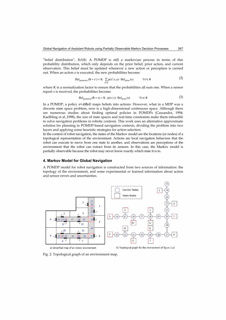
Fig. 2. Topological graph of an environment map.


Taking into account that the final objective of the SIRAPEM navigation system is to direct the robot from one room to another to perform guiding or service tasks, we discretize the environment into coarse-grained regions (nodes) of variable size in accordance with the topology of the environment, in order to make easier the planning task. As it’s shown in figure 2 for a virtual environment, only one node is assigned to each room, while the corridor is discretized into thinner regions. The limits of these regions correspond to any change in lateral features of the corridor (such as a new door, opening or piece of wall). This is a suitable discretization method in this type of structured environments, since nodes are directly related to topological locations in which the planning module may need to change the commanded action.

4.1. The elements of the Markov model: states, actions and observations

States (S) of the Markov model are directly related to the nodes of the topological graph. A single state corresponds to each room node, while four states are assigned to each corridor node, one for each of the four orientations the robot can adopt. The actions (A) selected to produce transitions from one state to another correspond to local navigation behaviors of the robot. We assume imperfect actions, so the effect of an action can be different of the expected one (this will be modeled by the transition model T). These actions are:

(1) “Go out room” (aO): to traverse door using sonar an visual information in room states,

(2) “Enter room” (aE): only defined in corridor states oriented to a door,

(3) “Turn right” (aR): to turn 90° to the right,

(4) “Turn Left” (aL): to turn 90° to the left, (5) “Follow Corridor” (aF): to continue through the corridor to the next state, and (6) “No Operation” (aNO): used as a directive in the goal state.

Finally, the observations (O) in our model come from the two sensorial systems of the robot: sonar and vision. Markov models provide a natural way to combine multisensorial information, as it will be shown in section 4.2.1. In each state, the robot makes three kind of observations:

(1) “Abstract Sonar Observation” (oASO). Each of the three nominal directions around the robot (left, front and right) is classified as “free” or “occupied” using sonar information, and an abstract observation is constructed from the combination of the percepts in each direction (thus, there are eight possible abstract sonar observations, as it’s shown in figure 3.a).

(2) “Landmark Visual Observation” (oLVO). Doors are considered as natural visual landmarks, because they exist in all indoor environments and can be easily segmented from the image using color (previously trained) and some geometrical restrictions. This observation is the number of doors (in lateral walls of the corridor) extracted from the image (see figure 3.b), and it reduces the perceptual aliasing of sonar by distinguishing states at the beginning from states at the end of a corridor. However, in long corridors, doors far away from the robot can’t be easily segmented from the image (this is the case of image 2 of figure 3.b), and this is the reason because we introduce a third visual observation.

(3) “Depth Visual Observation” (oDVO). As human-interaction robots have tall bodies with the camera on the top, it’s possible to detect the vanishing ceiling lines, and


classify its length into a set of discrete values (in this case, we use four quantification levels, as it’s shown in figure 3.b). This is a less sensitive to noise observation than using floor vanishing lines (mainly to occlusions due to people walking through the corridor), and provides complementary information to oLVO.

Figure 3.b shows two scenes of the same corridor from different positions, and their corresponding oLVO and oDVO observations. It’s shown that these are obtained by means of very simple image processing techniques (color segmentation for oLVO and edge detection for oDVO),and have the advantage, regarding correlation techniques used in (Gechter et al., 2001) or (Regini et al., 2002), that they are less sensitive to slight pose deviations within the same node.

Fig. 3. Observations of the proposed Markov model.

4.2. Visual information utility and improvements

Visual observations increase the robustness of the localization system by reducing perceptual aliasing. On the other hand, visual information also improves state transition detection, as it’s shown in the following subsections.

4.2.1. Sensor fusion to improve observability

Using only sonar to perceive the environment makes the Markov model highly non-observable due to perceptual aliasing. Furthermore, the “Abstract Sonar Observation” is highly dependent on doors state (opened or closed). The addition of the visual observations proposed in this work augments the observability of states. For example, corridor states with an opened door on the left and a wall on the right produces the same abstract sonar observation (oASO=1) independently if they are at the beginning or at the end of the corridor. However, the number of doors seen from the current state (oLVO)allows to distinguish between these states. POMDPs provide a natural way for using multisensorial fusion in their observation models (p(o|s) probabilities). In this case, o is a vector composed by the three observations proposed in the former subsection. Because these are independent observations, the observation model can be simplified in the following way:

)|p()|p()|p()|,,p()|p( sosososoooso DVOLVOASODVOLVOASO == (4)


4.2.2. Visual information to improve state transition detection

To ensure that when the robot is in a corridor, it only adopts the four allowed directions without large errors, it’s necessary that, during the execution of a “Follow Corridor” action, the robot becomes aligned with the corridor longitudinal axis. So, when the robot stands up to a new corridor, it aligns itself with a subtask that uses visual vanishing points, and during corridor following, it uses sonar buffers to detect the walls and construct a local model of the corridor. Besides, an individual “Follow Corridor” action terminates when the robot eaches a new state of the corridor. Detecting these transitions only with sonar readings is very critical when doors are closed. To solve this problem, we add visual information to detect door frames as natural landmarks of state transitions (using color segmentation and some geometrical restrictions). The advantage of this method is that the image processing step is fast and easy, being only necessary to process two lateral windows of the image as it’s shown in figure 4.

Fig. 4. State transition detection by means of visual information.

Whenever a vertical transition from wall to door color (or vice versa) is detected in a lateral window, the distance to travel as far as that new state is obtained from the following formula, using a pin-hole model of the camera (see figure 4):

( )lK

tg

ld ⋅=

α= (5)

where l is the distance of the robot to the wall in the same side as the detected door frame

(obtained from sonar readings) and α is the visual angle of the door frame. As the detected

frame is always in the edge of the image, the visual angle α only depends on the focal distance of the camera, that is constant for a fixed zoom (and known from camera specifications). After covering distance d (measured with relative odometry readings), the robot reaches the new state. This transition can be confirmed (fused) with sonar if the door is opened. Another advantage of this transition detection approach is that no assumptions are made about doors or corridor widths.


4.3. Action and observation uncertainties

Besides the topology of the environment, it’s necessary to define some action and observation uncertainties to generate the final POMDP model (transition and observation matrixes). A first way of defining these uncertainties is by introducing some experimental “hand-made” rules (this method is used in (Koenig & Simmons, 1998) and (Zanichelli, 1999)). For example, if a “Follow” action (aF) is commanded, the expected probability of making a state transition (F) is 70%, while there is a 10% probability of remaining in the same state (N=no action), a 10% probability of making two successive state transitions (FF), and a 10% probability of making three state transitions (FFF). Experience with this method has shown it to produce reliable navigation. However, a limitation of this method is that some uncertainties or parameters of the transition and observation models are not intuitive for being estimated by the user. Besides, results are better when probabilities are learned to more closely reflect the actual environment of the robot. So, our proposed learning module adjusts observation and transition probabilities with real data during an initial exploration stage, and maintains these parameters updated when the robot is performing another guiding or service tasks. This module, that also makes easier the installation of the system in new environments, is described in detail in section 8.

5. Navigation System Architecture

The problem of acting in partially observable environments can be decomposed into two components: a state estimator, which takes as input the last belief state, the most recent action and the most recent observation, and returns an updated belief state, and a policy, which maps belief states into actions. In robotics context, the first component is robot localization and the last one is task planning. Figure 5 shows the global navigation architecture of the SIRAPEM project, formulated as a POMDP model. At each process step, the planning module selects a new action as a command for the local navigation module, that implements the actions of the POMDP as local navigation behaviors. As a result, the robot modifies its state (location), and receives a new observation from its sensorial systems. The last action executed, besides the new observation perceived, are used by the localization module to update the belief distribution Bel(S).

Fig. 5. Global architecture of the navigation system.


After each state transition, and once updated the belief, the planning module chooses the next action to execute. Instead of using an optimal POMDP policy (that involves high computational times), this selection is simplified by dividing the planning module into two layers:

• A local policy, that assigns an optimal action to each individual state (as in the MDP case). This assignment depends on the planning context. Three possible contexts have been considered: (1) guiding (the objective is to reach a goal room selected by the user to perform a service or guiding task), (2) localizing (the objective is to reduce location uncertainty) and (3) exploring (the objective is to learn or adjust observations and uncertainties of the Markov model).

• A global policy, that using the current belief and the local policy, selects the best action by means of different heuristic strategies proposed by (Kaelbling et al., 1996).

This proposed two-layered planning architecture is able to combine several contexts of the local policy to simultaneously integrate different planning objectives, as will be shown in subsequent sections. Finally, the learning module (López et al., 2004) uses action and observation data to learn and adjust the observations and uncertainties of the Markov model.

6. Localization and Uncertainty Evaluation

The localization module updates the belief distribution after each state transition, using the well known Markov localization equations (2) and (3). In the first execution step, the belief distribution can be initialized in one of the two following ways: (a) If initial state of the robot is known, that state is assigned probability 1 and the rest 0, (b) If initial state is unknown, a uniform distribution is calculated over all states. Although the planning system chooses the action based on the entire belief distribution, in some cases it´s necessary to evaluate the degree of uncertainty of that distribution (this is, the locational uncertainty). A typical measure of discrete distributions uncertainty is the entropy. The normalized entropy (ranging from 0 to 1) of the belief distribution is:

)log(

))(log()(

)(Hs

s

n

sBelsBel∈

⋅−= S

Bel (6)

where ns is the number of states of the Markov model. The lower the value, the more certain the distribution. This measure has been used in all previous robotic applications for characterizing locational uncertainty (Kaelbling, 1996; Zanichelli, 1999). However, this measure is not appropriate for detecting situations in which there are a few maximums of similar value, being the rest of the elements zero, because it’s detected as a low entropy distribution. In fact, even being only two maximums, that is a not good result for the localization module, because they can correspond to far locations in the environment. A more suitable choice should be to use a least square measure respect to ideal delta distribution, that better detects the convergence of the distribution to a unique maximum (and so, that the robot is globally localized). However, we propose another approximate measure that, providing similar results to least squares, is faster calculated by using only the two first maximum values of the distribution (it’s also less sensitive when uncertainty is high, and more sensitive to secondary maximums during the tracking stage). This is the normalized divergence factor, calculated in the following way:

( )12

11)(D maxmax

−⋅

−+−=

s

s

n

pdnBel

(7)


where dmax is the difference between first and second maximum values of the distribution, and pmax the absolute value of the first maximum. Again, a high value indicates that the distribution converges to a unique maximum. In the results section we’ll show that this new measure provides much better results when planning in some kind of environments.

7. Planning under Uncertainty

A POMDP model is a MDP model with probabilistic observations. Finding optimal policies in the MDP case (that is a discrete space model) is easy and quickly for even very large models. However, in the POMDP case, finding optimal control strategies is computationally intractable for all but the simplest environments, because the beliefs space is continuous and high-dimensional. There are several recent works that use a hierarchical representation of the environment, with different levels of resolution, to reduce the number of states that take part in the planning algorithms (Theocharous & Mahadevan, 2002; Pineau & Thrun, 2002). However, these methods need more complex perception algorithms to distinguish states at different levels of abstraction, and so they need more prior knowledge about the environment and more complex learning algorithms. On the other hand, there are also several recent approximate methods for solving POMDPs, such as those that use a compressed belief distribution to accelerate algorithms (Roy, 2003) or the ‘point-based value iteration algorithm’ (Pineau et al., 2003) in which planning is performed only on a sampled set of reachable belief points. The solution adopted in this work is to divide the planning problem into two steps: the first

one finds an optimal local policy for the underlying MDP (a*=π*(s), or to simplify notation, a*(s)), and the second one uses a number of simple heuristic strategies to select a final action (a*(Bel)) as a function of the local policy and the belief. This structure is shown in figure 6 and described in subsequent subsections.

Global POMDP Policy

Bel(S)

Local MDP Policies

a*(Bel)

PLANNING SYSTEM

Context Selection

Guidance Context

Localization

Context

Exploration

Context

Action

aG*(s) aL*(s) aE*(s)

a*(s)

Goal room

Fig. 6. Planning system architecture, consisting of two layers: (1) Global POMDP policy and (2) Local MDP policies.

7.1. Contexts and local policies

The objective of the local policy is to assign an optimal action (a*(s)) to each individual state s. This assignment depends on the planning context. The use of several contexts allows the


robot to simultaneously achieve several planning objectives. The localization and guidance contexts try to simulate the optimal policy of a POMDP, which seamlessly integrates the two concerns of acting in order to reduce uncertainty and to achieve a goal. The exploration context is to select actions for learning the parameters of the Markov model. In this subsection we show the three contexts separately. Later, they will be automatically selected or combined by the ‘context selection’ and ‘global policy’ modules (figure 6).

7.1.1. Guidance Context

This local policy is calculated whenever a new goal room is selected by the user. Its main objective is to assign to each individual state s, an optimal action (aG*(s)) to guide the robot to the goal. One of the most well known algorithms for finding optimal policies in MDPs is ’value iteration’ (Bellman, 1957). This algorithm assigns an optimal action to each state when the reward function r(s,a) is available. In this application, the information about the utility of actions for reaching the destination room is contained in the graph. So, a simple path searching algorithm can effectively solve the underlying MDP, without any intermediate reward function. So, a modification of the A* search algorithm (Winston, 1984) is used to assign a preferred heading to each node of the topological graph, based on minimizing the expected total number of nodes to traverse (shorter distance criterion cannot be used because the graph has not metric information). The modification of the algorithm consists of inverting the search direction, because in this application there is not an initial node (only a destination node). Figure 7 shows the resulting node directions for goal room 2 on the graph of environment of figure 2.

Fig. 7. Node directions for “Guidence” (to room 2) and “Localization” contexts for environment of figure 2.

Later, an optimal action is assigned to the four states of each node in the following way: a “follow” (aF) action is assigned to the state whose orientation is the same as the preferred heading of the node, while the remaining states are assigned actions that will turn the robot towards that heading (aL or aR). Finally, a “no operation” action (aNO) is assigned to the goal room state. Besides optimal actions, when a new goal room is selected, Q(s,a) values are assigned to each (s,a) pair. In the MDPs theory, Q-values (Lovejoi, 1991) characterize the utility of executing each action at each state, and will be used by one of the global heuristic policies shown in next subsection. To simplify Q-values calculation, the following criterion has been used: Q(s,a)=1 if action a is optimal at state s, Q(s,a)=-1 (negative utility) if actions a is not


defined at state s, and Q(s,a)=-0.5 for the remaining cases (actions that disaligns the robot from the preferred heading).

7.1.2. Localization Context

This policy is used to guide the robot to “Sensorial Relevant States“ (SRSs) that reduce positional uncertainty, even if that requires moving it away from the goal temporarily. This planning objective was not considered in previous similar robots, such as DERVISH (Nourbakhsh et al., 1995) or Xavier (Koenig & Simmons, 1998), or was implemented by means of fixed sequences of movements (Cassandra, 1994) that don’t contemplate environment relevant places to reduce uncertainty. In an indoor environment, it’s usual to find different zones that produce not only the same observations, but also the same sequence of observations as the robot traverses them by executing the same actions (for example, symmetric corridors). SRSs are states that break a sequence of observations that can be found in another zone of the graph. Because a state can be reached from different paths and so, with different histories of observations, SRSs are not characteristic states of the graph, but they depend on the starting state of the robot. This means that each starting state has its own SRS. To simplify the calculation of SRSs, and taking into account that the more informative states are those aligned with corridors, it has been supposed that in the localization context the robot is going to execute sequences of “follow corridor” actions. So, the moving direction along the corridor to reach a SRS as soon as possible must be calculated for each state of each corridor. To do this, the “Composed Observations“ (COs) of these states are calculated from the graph and the current observation model ϑ in the following way:

( ) )

( ) )

( ) )s|o(pmaxarg)s(o

s|o(pmaxarg)s(o

s|o(pmaxarg)s(owith

)s(o)s(o10)s(o100)s(CO

ASOASOO

ASO

LVOLVOO

LVO

DVODVOO

DVO

ASOLVODVO

=

=

=

+⋅+⋅= (8)

Later, the nearest SRS for each node is calculated by studying the sequence of COs obtained while moving in both corridor directions. Then, a preferred heading (among them that align the robot with any connected corridor) is assigned to each node. This heading points at the corridor direction that, by a sequence of “Follow Corridor” actions, directs the robot to the nearest SRS (figure 7 shows the node directions obtained for environment of figure 2). And finally, an optimal action is assigned to the four states of each corridor node to align the robot with this preferred heading (as it was described in the guidance context section). The optimal action assigned to room states is always “Go out room” (aO).So, this policy (a*L(s)) is only environment dependent and is automatically calculated from the connections of the graph and the ideal observations of each state.

7.1.3. Exploration Context

The objective of this local policy is to select actions during the exploration stage, in order to learn transition and observation probabilities. As in this stage the Markov model is unknown (the belief can’t be calculated), there is not distinction between local and global policies, whose common function is to select actions in a reactive way to explore the


environment. As this context is strongly connected with the learning module, it will be explained in section 8.

7.2. Global heuristic policies

The global policy combines the probabilities of each state to be the current state (belief distribution Bel(S)) with the best action assigned to each state (local policy a*(s)) to select the final action to execute, a*(Bel). Once selected the local policy context (for example guidance context, a*(s)=aG*(s)), some heuristic strategies proposed by (Kaelbling et al., 1996) can be used to do this final selection. The simpler one is the “Most Likely State“ (MLS) global policy that finds the state with the highest probability and directly executes its local policy:

( )= )(maxarg*)(* sBelaas

MLS Bel(9)

The “Voting“ global policy first computes the “probability mass” of each action (V(a))(probability of action a being optimal) according to the belief distribution, and then selects the action that is most likely to be optimal (the one with highest probability mass):

( ))(maxarg)(

)()(

*

)(*

aVBela

asBelaV

avot

sasa

=

∈∀==

A(10)

This method is less sensitive to locational uncertainty, because it takes into account all states, not only the most probable one. Finally, the QMDP global policy is a more refined version of the voting policy, in which the votes of each state are apportioned among all actions according to their Q-values:

( ))(maxarg)(

)()()(

* aVBela

asQsBelaV

aQ

a

Ss

MDP=

∈∀⋅=∈

A(11)

This is in contrast to the “winner take all” behavior of the voting method, taking into account negative effect of actions. Although there is some variability between these methods, for the most part all of them do well when initial state of the robot is known, and only the tracking problem is present. If initial state is unknown, the performance of the methods highly depends on particular configuration of starting states. However, MLS or QMDP global policies may cycle through the same set of actions without progressing to the goal when only guidance context is used. Properly combination of guidance and localization context highly improves the performance of these methods during global localization stage.

7.3. Automatic context selection or combination

Apart from the exploration context, this section considers the automatic context selection (see figure 6) as a function of the locational uncertainty. When uncertainty is high, localization context is useful to gather information, while with low uncertainty, guidance context is the appropriate one. In some cases, however, there is benign high uncertainty in the belief state; that is, there is confusion among states that requires the same action. In these cases, it’s not necessary to commute to localization context. So, an appropriate measure of


uncertainty is the “normalized divergence factor“ of the probability mass distribution, D(V(a)), (see eq. 7).

The “thresholding-method“ for context selection uses a threshold φ for the divergence factor D. Only when divergence is over that threshold (high uncertainty), localization context is used as local policy:

φ≥

φ<=

Dsisa

Difsasa

L

G

)(

)()(*

*

*

(12)

However, the “weighting-method“ combines both contexts using divergence as weighting factor. To do this, probability mass distributions for guidance and localization contexts (VG(a) and VL(a))are computed separately, and the weighted combined to obtain the final probability mass V(a). As in the voting method, the action selected is the one with highest probability mass:

))((maxarg)(*

)()()1()(

aVBela

sVDaVDaV

a

LG

=

⋅+⋅−= (13)

8. Learning the Markov Model of a New Environment

The POMDP model of a new environment is constructed from two sources of information:

• The topology of the environment, represented as a graph with nodes and

connections. This graph fixes the states (s ∈ S) of the model, and establishes the ideal transitions among them by means of logical connectivity rules.

• An uncertainty model, that characterizes the errors or ambiguities of actions and observations, and together with the graph, makes possible to generate the

transition T and observation ϑ matrixes of the POMDP. Taking into account that a reliable graph is crucial for the localization and planning systems to work properly, and the topological representation proposed in this work is very close to human environment perception, we propose a manual introduction of the graph. To do this, the SIRAPEM system incorporates an application to help the user to introduce the graph of the environment (this step is needed only once when the robot is installed in a new working domain, because the graph is a static representation of the environment).

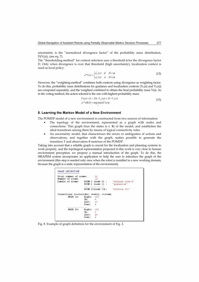
Fig. 8. Example of graph definition for the environment of Fig. 2.


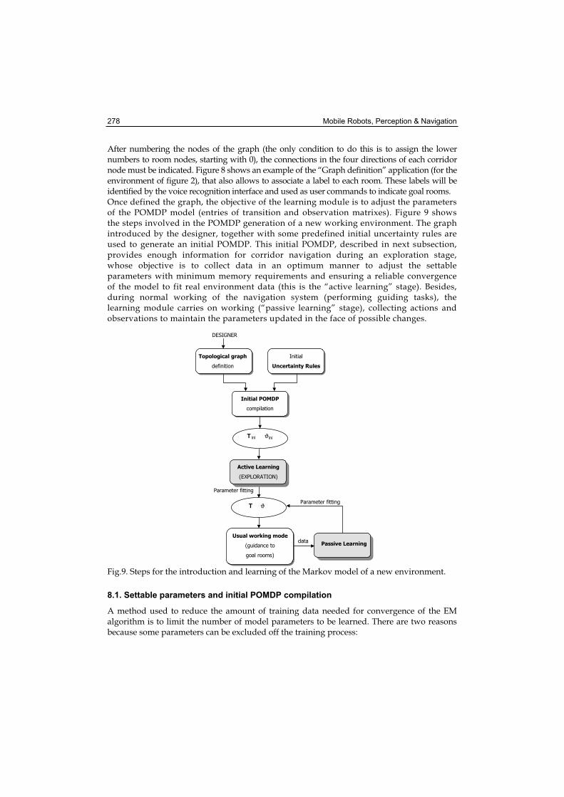
After numbering the nodes of the graph (the only condition to do this is to assign the lower numbers to room nodes, starting with 0), the connections in the four directions of each corridor node must be indicated. Figure 8 shows an example of the “Graph definition” application (for the environment of figure 2), that also allows to associate a label to each room. These labels will be identified by the voice recognition interface and used as user commands to indicate goal rooms. Once defined the graph, the objective of the learning module is to adjust the parameters of the POMDP model (entries of transition and observation matrixes). Figure 9 shows the steps involved in the POMDP generation of a new working environment. The graph introduced by the designer, together with some predefined initial uncertainty rules are used to generate an initial POMDP. This initial POMDP, described in next subsection, provides enough information for corridor navigation during an exploration stage, whose objective is to collect data in an optimum manner to adjust the settable parameters with minimum memory requirements and ensuring a reliable convergence of the model to fit real environment data (this is the “active learning” stage). Besides, during normal working of the navigation system (performing guiding tasks), the learning module carries on working (“passive learning” stage), collecting actions and observations to maintain the parameters updated in the face of possible changes.

Usual working mode

(guidance to

goal rooms)

Active Learning

(EXPLORATION)

Topological graph

definition

DESIGNER

Initial

Uncertainty Rules

Initial POMDP

compilation

T ini ϑini

T ϑ

Passive Learning

Parameter fitting

Parameter fitting

data

Fig.9. Steps for the introduction and learning of the Markov model of a new environment.

8.1. Settable parameters and initial POMDP compilation

A method used to reduce the amount of training data needed for convergence of the EM algorithm is to limit the number of model parameters to be learned. There are two reasons because some parameters can be excluded off the training process:


• Some parameters are only robot dependent, and don’t change from one environment to another. Examples of this case are the errors in turn actions (that are nearly deterministic due to the accuracy of odometry sensors in short turns), or errors of sonars detecting “free” when “occupied” or vice versa.

• Other parameters directly depend on the graph and some general uncertainty rules, being possible to learn the general rules instead of its individual entries in the model matrixes. This means that the learning method constrains some probabilities to be identical, and updates a probability using all the information that applies to any probability in its class. For example, the probability of losing a transition while following a corridor can be supposed to be identical for all states in the corridor, being possible to learn the general probability instead of the particular ones.

Taking these properties into account, table 1 shows the uncertainty rules used to generate the initial POMDP in the SIRAPEM system.

Table 1. Predefined uncertainty rules for constructing the initial POMDP model.

Figure 10 shows the process of initial POMDP compilation. Firstly, the compiler automatically assigns a number (ns) to each state of the graph as a function of the number of the node to which it belongs (n) and its orientation within the node (head={0(right), 1(up), 2(left), 3(down)}) in the following way (n_rooms being the number of room nodes):


Room states: ns=nCorridor states: ns=n_rooms+(n-n_rooms)*4+head

Fig. 10. Initial POMDP compilation, and structure of the resulting transition and observation matrixes. Parameters over gray background will be adjusted by the learning system.


Finally, the compiler generates the initial transition and observation matrixes using the predefined uncertainty rules. Settable parameters are shown over gray background in figure 10, while the rest of them will be excluded of the training process. The choice of settable parameters is justified in the following way:

• Transition probabilities. Uncertainties for actions “Turn Left” (aL), “Turn Right” (aR),“Go out room” (aO) and “Enter room” (aE) depends on odometry and the developed algorithms, and can be considered environment independent. However, the “Follow corridor” (aF) action highly depends on the ability of the vision system to segment doors color, that can change from one environment to another. As a pessimistic initialization rule, we use a 70% probability of making the ideal “follow” transition (F), and 10% probabilities for autotransition (N), and two (FF) or three (FFF) successive transitions, while the rest of possibilities are 0. However, these probabilities will be adjusted by the learning system to better fit real environment conditions. In this case, instead of learning each individual transition probability, the general rule (values for N, F, FF and FFF) will be trained (so, transitions that initially are 0 will be kept unchanged). The new learned values are used to recompile the rows of the transition matrix corresponding to corridor states aligned with corridor directions (the only ones in which the “Follow Corridor” action is defined).

• Observation probabilities. The Abstract Sonar Observation can be derived from the graph, the state of doors, and a model of the sonar sensor characterizing its probability of perceiving “occupied” when “free” or vice versa. The last one is no environment dependent, and the state of doors can change with high frequency. So, the initial model contemplates a 50% probability for states “closed” and “opened” of all doors. During the learning process, states containing doors will be updated to provide the system with some memory about past state of doors. Regarding the visual observations, it’s obvious that they are not intuitive for being predefined by the user or deduced from the graph. So, in corridor states aligned with corridor direction, the initial model for both visual observations consists of a uniform distribution, and the probabilities will be later learned from robot experience during corridor following in the exploration stage.

As a resume, the parameters to be adjusted by the learning system are: • The general rules N, F, FF and FFF for the “Follow Corridor” action. Their initial

values are shown in table I. • the probabilities for the Abstract Sonar Observation of corridor states in which there is a

door in left, right or front directions (to endow the system with some memory about past door states, improving the localization system results). Initially, it’s supposed a 50% probability for “opened” and “closed” states. In this case, the adjustment will use a low gain because the state of doors can change with high frequency.

• The probabilities for the Landmark Visual Observation and Deep Visual Observation of corridor states aligned with corridor direction, that are initialized as uniform distributions.

8.2. Training data collection

Learning Markov models of partially observable environments is a hard problem, because it involves inferring the hidden state at each step from observations, as well as estimating the transition and observation models, while these two procedures are mutually dependent.


The EM algorithm (in Hidden Markov Models context known as Baum-Welch algorithm) is

an expectation-maximization algorithm for learning the parameters (entries of the transition

and observation probabilistic models) of a POMDP from observations (Bilmes, 1997). The

input for applying this method is an execution trace, containing the sequence of actions-

observations executed and collected by the robot at each execution step t=1...T (T is the total

number of steps of the execution trace):

[ ]T1T1Ttt2211

o,a,o,...,a,o,...,a,o,a,o −−=trace (14)

The EM algorithm is a hill-climbing process that iteratively alternates two steps to converge

to a POMDP that locally best fits the trace. In the E-Step (expectation step), probabilistic

estimates for the robot states (locations) at the various time steps are estimated based on the

currently available POMDP parameters (in the first iteration, they can be uniform matrixes).

In the M-Step (maximization step), the maximum likelihood parameters are estimated based

on the states computed in the E-step. Iterative application of both steps leads to a refinement

of both, state estimation, and POMDP parameters.

The limitations of the standard EM algorithm are well known. One of them is that it converges to a

local optimum, and so, the initial POMDP parameters have some influence on the final learned

POMDP. But the main disadvantage of this algorithm is that it requires a large amount of training

data. As the degrees of freedom (settable parameters) increase, so does the need for training data.

Besides, in order to the algorithm to converge properly, and taking into account that EM is in

essence a frequency-counting method, the robot needs to traverse several times de whole

environment to obtain the training data. Given the relative slow speed at which mobile robots can

move, it’s desirable that the learning method learns good POMDP models with as few corridor

traversals as possible. There are some works proposing alternative approximations of the

algorithm to lighten this problem, such as (Koening & Simmons, 1996) or (Liu et al., 2001). We

propose a new method that takes advantage of human-robot interfaces of assistant robots and the

specific structure of the POMDP model to reduce the amount of data needed for convergence.

To reduce the memory requirements, we take advantage of the strong topological

restrictions of our POMDP model in two ways:

• All the parameters to be learned (justified in the last subsection) can be obtained

during corridor following by sequences of “Follow Corridor” actions. So, it’s not

necessary to alternate other actions in the execution traces, apart from turn actions

needed to start the exploration of a new corridor (that in any case will be excluded

off the execution trace).

• States corresponding to different corridors (and different directions within the

same corridor) can be broken up from the global POMDP to obtain reduced sub-

POMDPs. So, a different execution trace will be obtained for each corridor and each

direction, and only the sub-POMDP corresponding to the involved states will be

used to calculate de EM algorithm, reducing in this way the memory requirements.

As it was shown in figure 9, there are two learning modes, that also differ in the way in

which data is collected: the active learning mode during an initial exploration stage, and the

passive learning mode during normal working of the navigation system.


8.2.1. Supervised active learning. Corridors exploration

The objective of this exploration stage is to obtain training data in an optimized way to

facilitate the initial adjustment of POMDP parameters, reducing the amount of data of

execution traces, and the number of corridor traversals needed for convergence. The

distinctive features of this exploration process are:

• The objective of the robot is to explore (active learning), and so, it independently

moves up and down each corridor, collecting a different execution trace for each

direction. Each corridor is traversed the number of times needed for the proper

convergence of the EM algorithm (in the results section it will be demonstrated that

the number of needed traversals ranges from 3 to 5).

• We introduce some user supervision in this stage, to ensure and accelerate

convergence with a low number of corridor traversals. This supervision can be

carried out by a non expert user, because it consists in answering some questions

the robot formulates during corridor exploration, using the speech system of the

robot. To start the exploration, the robot must be placed in any room of the corridor

to be explored, whose label must be indicated with a talk as the following:

Robot: I’m going to start the exploration. ¿Which is the initial room?

Supervisor: dinning room A

Robot: Am I in dinning room A?

Supervisor: yes

With this information, the robot initializes its belief Bel(S) as a delta distribution centered in

the known initial state. As the initial room is known, states corresponding to the corridor to

be explored can be extracted from the graph, and broken up from the general POMDP as it’s

shown in figure 11. After executing an “Out Room” action, the robot starts going up and

down the corridor, collecting the sequences of observations for each direction in two

independent traces (trace 1 and trace 2 of figure 11). Taking advantage of the speech system,

some “certainty points” (CPs) are introduced in the traces, corresponding to initial and final

states of each corridor direction. To obtain these CPs, the robot asks the user “Is this the end

state of the corridor?” when the belief of that final state is higher than a threshold (we use a

value of 0.4). If the answer is “yes”, a CP is introduced in the trace (flag cp=1 in figure 11),

the robot executes two successive turns to change direction, and introduces a new CP

corresponding to the initial state of the opposite direction. If the answer is “no”, the robot

continues executing “Follow Corridor” actions. This process is repeated until traversing the

corridor a predefined number of times.

Figure 11 shows an example of exploration of the upper horizontal corridor of the

environment of figure 2, with the robot initially in room 13. As it’s shown, an

independent trace is stored for each corridor direction, containing a header with the

number of real states contained in the corridor, its numeration in the global POMDP,

and the total number execution steps of the trace. The trace stores, for each execution

step, the reading values of ASO, LVO and DVO, the “cp” flag indicating CPs, and their

corresponding “known states”. These traces are the inputs for the EM-CBP algorithm

shown in the next subsection.


Fig. 11. Example of exploration of one of the corridors of the environment of figure 2 (involved nodes, states of the two execution traces, and stored data).

8.2.2. Unsupervised passive learning

The objective of the passive learning is to keep POMDP parameters updated during the normal working of the navigation system. These parameters can change, mainly the state of doors (that affects the Abstract Sonar Observation), or the lighting conditions (that can modify the visual observations or the uncertainties of “Follow Corridor” actions). Because during the normal working of the system (passive learning), actions are not selected to optimize execution traces (but to guide the robot to goal rooms), the standard EM algorithm must be applied. Execution traces are obtained by storing sequences of actions and observations during the navigation from one room to another. Because they usually correspond to only one traversal of the route, sensitivity of the learning algorithm must be lower in this passive stage, as it’s explained in the next subsection.


Fig. 12. Extraction of the local POMDP corresponding to one direction of the corridor to be explored.

8.3. The EM-CBP Algorithm

The EM with Certainty Break Points (EM-CBP) algorithm proposed in this section can be

applied only in the active exploration stage, with the optimized execution traces. In this

learning mode, an execution trace corresponds to one of the directions of a corridor, and

involves only “Follow Corridor” actions.

The first step to apply the EM-CBP to a trace is to extract the local POMDP corresponding to

the corridor direction from the global POMDP, as it’s shown in figure 12. To do this, states

are renumbering from 0 to n-1 (n being the number of real states of the local POMDP). The

local transition model Tl contains only the matrix corresponding to the “Follow Corridor”

action (probabilities p(s’|s,aF), whose size for the local POMDP is (n-1)x(n-1), and can be

constructed from the current values of N, F, FF and FFF uncertainty rules (see figure 12).

The local observation model ϑl also contains only the involved states, extracted from the

global POMDP, as it’s shown in figure 12.


The main distinguishing feature of the EM with Certainty Break Points algorithm is that it

inserts delta distributions in alfa and beta (and so, gamma) distributions of the standard EM

algorithm, corresponding to time steps with certainty points. This makes the algorithm to

converge in a more reliable and fast way with shorter execution traces (and so, less corridor

traversals) than the standard EM algorithm, as will be demonstrate in the results section.

Figure 13 shows the pseudocode of the EM-CBP algorithm. The expectation and

maximization steps are iterated until convergence of the estimated parameters. The

stopping criteria is that all the settable parameters remain stable between iterations (with

probability changes lower than 0.05 in our experiments).

The update equations shown in figure 13 (items 2.4 and 2.5) differ from the standard EM in

that they use Baye’s rule (Dirichlet distributions) instead of frequencies. This is because,

although both methods produce asymptotically the same results for long execution traces,

frequency-based estimates are not very reliable if the sample size is small. So, we use the

factor K (K>0) to indicate the confidence in the initial probabilities (the higher the value, the

higher the confidence, and so, the lower the variations in the parameters). The original re-

estimation formulas are a special case with K=0. Similarly, leaving the transition

probabilities unchanged is a special case with K→∞.

Fig. 13. Pseudocode of the EM-CBP algorithm.


In practice, we use different values of K for the different settable parameters. For example, as visual observations are uniformly initialized, we use K=0 (or low values) to allow convergence with a low number of iterations. However, the adjustment of Abstract Sonar Observations corresponding to states with doors must be less sensitive (we use K=100), because the state of doors can easily change, and all the probabilities must be contemplated with relative high probability. During passive learning we also use a high value of K (K=500), because in this case the execution traces contain only one traversal of the route, and some confidence about previous values must be admitted. The final step of the EM-CBP algorithm is to return the adjusted parameters from the local POMDP to the global one. This is carried out by simple replacing the involved rows of the global POMDP with their corresponding rows of the learned local POMDP.

9. Results

To validate the proposed navigation system and test the effect of the different involved parameters, some experimental results are shown. Because some statistics must be extracted and it’s also necessary to validate the methods in real robotic platforms and environments, two kind of experiments are shown. Firstly, we show some results obtained with a simulator of the robot in the virtual environment of figure 2, in order to extract some statistics without making long tests with the real robotic platform. Finally, we´ll show some experiments carried out with the real robot of the SIRAPEM project in one of the corridors of the Electronics Department.

9.1. Simulation results

The simulation platform used in these experiments (figure 14) is based on “Saphira” commercial software (Konolige & Myers, 1998) provided by ActivMedia Robotics, that includes a very realistic robot simulator, that very closely reproduces real robot movements and ultrasound noisy measures on a user defined map. A visual 3D simulator using OpenGL software has been added to incorporate visual observations. Besides, to test the algorithms in extreme situations, we have incorporated to the simulator some methods to increase the non-ideal effect of actions, and noise in observations (indeed, these are higher that in real environment tests). So, simulation results can be reliably extrapolated to extract realistic conclusions about the system.

Fig. 14. Diagram of test platforms: real robot and simulator.


There are some things that make one world more difficult to navigate than another. One of them is its degree of perceptual aliasing, that substantially affects the agent’s ability for localization and planning. The localization and two-layered planning architecture proposed in this work improves the robustness of the system in typical “aliased” environments, by properly combining two planning contexts: guidance and localization. As an example to demonstrate this, we use the virtual aliased environment shown in figure 2, in which there are two identical corridors. Firstly, we show some results about the learning system, then some results concerning only the localization system are shown and finally we include the planning module in some guidance experiments to compare the different planning strategies.

9.1.1. Learning results

The objective of the first simulation experiment is to learn the Markov model of the sub-POMDP corresponding to the upper horizontal corridor of the environment of figure 2, going from left to right (so, using only the trace 1 of the corridor). Although the global graph yields a POMDP with 94 states, the local POMDP corresponding to states for one direction of that corridor has 7 states (renumbered from 0 to 6), and so, the sizes of the local matrixes are: 7x7 for the transition matrix p(s’|s,aF), 7x4 for the Deep Visual Observation matrix p(oDVO|s), and 7x8 for the Abstract Sonar Observation matrix p(oASO|s). The Landmark Visual Observation has been excluded off the simulation experiments to avoid overloading the results, providing similar results to the Deep Visual Observation. In all cases, the initial POMDP was obtained using the predefined uncertainty rules of table 1. The simulator establishes that the “ideal” model (the learned model should converge to it) is that shown in table 2. It shows the “ideal” D.V.O. and A.S.O. for each local state (A.S.O. depends on doors states), and the simulated non-ideal effect of “Follow Corridor” action, determined by uncertainty rules N=10%, F=80%, FF=5% and FFF=5%.

Table 2. Ideal local model to be learned for upper horizontal corridor of figure 2.

In the first experiment, we use the proposed EM-CBP algorithm to simultaneously learn the “follow corridor” transition rules, D.V.O. observations, and A.S.O. observations (all doors were closed in this experiment, being the worst case, because the A.S.O doesn’t provide information for localization during corridor following). The corridor was traversed 5 times to obtain the execution trace, that contains a CP at each initial and final state of the corridor, obtained by user supervision. Figure 15 shows the learned model, that properly fits the ideal parameters of table 2. Because K is large for A.S.O. probabilities adjustment, the learned model still contemplates the probability of doors being opened. The graph on the right of figure 15 shows a comparison between the real states that the robot traversed to obtain the execution trace, and the estimated states using the learned model, showing that the model properly fits the execution trace. Figure 16 shows the same results using the standard EM algorithm, without certainty points. All the conditions are identical to the last experiment, but the execution trace was


obtained by traversing the corridor 5 times with different and unknown initial and final positions. It’s shown that the learned model is much worse, and its ability to describe the execution trace is much lower.

Fig. 15. Learned model for upper corridor of figure 2 using the EM-CBP algorithm.

Fig. 16. Learned model for upper corridor of figure 2 using the standard EM algorithm.

Table 3 shows some statistical results (each experiment was repeated ten times) about the effect of the number of corridor traversals contained in the execution trace, and the state of doors, using the EM-CBP and the standard EM algorithms. Although there are several measures to determine how well the learning method converges, in this table we show the percentage of faults in estimating the states of the execution trace. Opened doors clearly improve the learned model, because they provide very useful information to estimate states in the expectation step of the algorithm (so, it’s a good choice to open all doors during the active exploration stage). As it’s shown, using the EM-CBP method with all doors opened


provides very good models even with only one corridor traversal. With closed doors, the EM-CBP needs between 3 and 5 traversals to obtain good models, while standard EM needs around 10 to produce similar results. In our experiments, we tested that the number of iterations for convergence of the algorithm is independent of all these conditions (number of corridor traversals, state of doors, etc.), ranging from 7 to 12.

EM-CBP Standard EM

Nº of corridor traversals

All doors closed

All doorsopened

All doors closed

All doors opened

1 37.6 % 6.0 % 57.0 % 10.2 %

2 19.5 % 0.6 % 33.8 % 5.2 %

3 13.7 % 0.5 % 32.2 % 0.8 %

5 12.9 % 0.0 % 23.9 % 0.1 %

10 6.7 % 0.0 % 12.6 % 0.0 %

Table 3. Statistical results about the effect of corridor traversals and state of doors.

9.1.2. Localization results

Two are the main contributions of this work to Markov localization in POMDP navigation systems. The first one is the addition of visual information to accelerate the global localization stage from unknown initial position, and the second one is the usage of a novel measure to better characterize locational uncertainty. To demonstrate them, we executed the trajectory shown in figure 17.a, in which the “execution steps” of the POMDP process are numbered from 0 to 11. The robot was initially at node 14 (with unknown initial position), and a number of “Follow corridor” actions were executed to reach the end of the corridor, then it executes a “Turn Left” action and continues through the new corridor until reaching room 3 door. In the first experiments, all doors were opened, ensuring a good transition detection. This is the best assumption for only sonar operation. Two simulations were executed in this case: the first one using only sonar information for transition detection and observation, and the second one adding visual information. As the initial belief is uniform, and there is an identical corridor to that in which the robot is, the belief must converge to two maximum hypotheses, one for each corridor. Only when the robot reaches node 20 (that is an SRS) is possible to eliminate this locational uncertainty, appearing a unique maximum in the distribution, and starting the “tracking stage”. Figure 17.b shows the real state assigned probability evolution during execution steps for the two experiments. Until step 5 there are no information to distinguish corridors, but it can be seen that with visual information the robot is better and sooner localized within the corridor. Figure 17.c shows entropy and divergence of both experiments. Both measures detect a lower uncertainty with visual information, but it can be seen that divergence better characterizes the convergence to a unique maximum, and so, the end of the global localization stage. So, with divergence it’s easier to establish a threshold to distinguish “global localization” and “tracking” stages. Figures 17.d and 17.e show the results of two new simulations in which doors 13, 2 and 4 were closed. Figure 17.d shows how using only sonar information some transitions are lost (the robots skips positions 3 , 9 and 10 of figure 17.a). This makes much worse the localization results. However, adding visual information no transitions are lost, and results are very similar to that of figure 17.b. So, visual information makes the localization more robust, reducing perceptual aliasing of


states in the same corridor, and more independent of doors state. Besides, the proposed divergence uncertainty measure better characterizes the positional uncertainty that the typical entropy used in previous works.

Fig. 17. Localization examples. (a) Real position of the robot at each execution step, (b) Bel(sreal) with all doors opened, with only sonar (__) and with sonar+vision (---), (c) uncertainty measures with all doors opened, (d) the same as (b) but with doors 13,2,4 closed, (e) the same as (c) but with doors 13,2,4 closed.


9.1.3. Planning Results

The two layered planning architecture proposed in this work improves the robustness of the system in “aliased” environments, by properly combining the two planning contexts: guidance and localization. To demonstrate this, we show the results after executing some simulations in the same fictitious environment of figure 17.a. In all the experiments the robot was initially at room state 0, and the commanded goal room state was 2. However, the only initial knowledge of the robot about its position is that it’s a room state ( initial belief is a uniform distribution over room states). So, after the “go out room” action execution, and thanks to the visual observations, the robot quickly localizes itself within the corridor, but due to the environment aliasing, it doesn’t know in which corridor it is. So, it should use the localization context to reach nodes 20 or 27 of figure 2, that are sensorial relevant nodes to reduce uncertainty.

ONLY GUIDANCE CONTEXT

Nº Actions Final H Final D Final State 2

MLS 6 0.351 0.754 54.3%

Voting 17 0.151 0.098 63.8%

QMDP 15 0.13 0.095 62.3%

GUIDANCE AND LOCALIZATION CONTEXTS (always with voting global method)

Nº Actions Final H Final D Final State 2

H(V(a)) threshold 14 0.13 0.05 83.5%

D(V(a)) threshold 13 0.12 0.04 100%

Weighted D(V(a)) 13 0.12 0.04 100%

Table 4. Comparison of the planning strategies in the virtual environment of figure 17.a.

Table 4 shows some statistical results (average number of actions to reach the goal, final values of entropy and divergence and skill percentage on reaching the correct room) after repeating each experiment a number of times. Methods combining guidance and localization contexts are clearly better, because they direct the robot to node 20 before acting to reach the destination, eliminating location uncertainty, whereas using only guidance context has a unpredictable final state between rooms 2 and 11. On the other hand, using the divergence factor proposed in this work, instead of entropy, improves the probability of reaching the correct final state, because it better detects the convergence to a unique maximum (global localization).

9.2. Real robot results

To validate the navigation system in larger corridors and real conditions, we show the results

obtained with SIRA navigating in one of the corridors of the Electronics Department of the

University of Alcalá. Figure 19 shows the corridor map and its corresponding graph with 71 states.

The first step to install the robot in this environment was to introduce the graph and explore

the corridor to learn the Markov model. The local POMDP of each corridor direction

contains 15 states. To accelerate convergence, all doors were kept opened during the active

exploration stage. We evaluated several POMDP models, obtained in different ways:

• The initial model generated by the POMDP compiler, in which visual observations of corridor aligned states are initialized with uniform distributions.

• A “hand-made” model, in which visual observations were manually obtained


(placing the robot in the different states and reading the observations).

• Several learned POMDP models (using the EM-CBP algorithm), with different number of corridor traversals (from one to nine) during exploration.

Two “evaluation trajectories” were executed using these different models to localize the robot. In the first one, the robot crossed the corridor with unknown initial position and all doors opened, and in the second one, all doors were closed. The localization system was able to global localize the robot in less than 5 execution steps in both cases with all models. However, the uncertainty of the belief distribution was higher with worse models. Figure 18 shows the mean entropy of the belief distribution for all the evaluation trajectories. The “initial POMDP model” is the worst, because it doesn’t incorporate information about visual observations. The learned model with one corridor traversal is not better that the “hand-made” one, but from two traversals, the obtained entropy and easy installation justifies the usage of the learning module. It can also be deduced that a good number of corridor traversals ranges from 2 to 4 in this case, because later adjustments of the model can be carried out during “active exploration”. Because all doors were opened during exploration, as the number of corridor traversals increases, so does the evidence about opened doors in the model and so, the uncertainty in the “evaluation trajectory” with opened doors decreases, while in that with closed doors increases. So, the model adapts this kind of environment changes. The time required for exploring one corridor with three traversals was about 5 minutes (with a medium speed of 0.3 m/s). The computation time of the EM-CBP algorithm, using the onboard PC of the robot (a 850MHz Pentium III) was 62 ms. These times are much lower that the ones obtained in Thrun’s work (Thrun et al., 1998 b), in which for learning a metric map of an environment of 60x60 meters (18 times larger than our corridor), an exploration time of 15 minutes and computation time of 41 minutes were necessary.

Fig. 18. Comparison of the mean entropy of the belief distribution using different models for the corridor to localize the robot in two evaluation trajectories.


Fig. 19. Topological graph model for a corridor of the Electronics Department, and executed trajectory from room 2 to room 4 (process evolution shown in table 5).

Once shown the results of the learning process, a guidance example is included in which robot was initially in room 2 with unknown initial room state, and room 4 was commanded as goal state (see figure 19).

10

20

30

40

50

60

70

80

90

Uniform

over rooms

The same for

13↑,16↑,

19↑,22↑,

12↓,15↓,18↓,21↓

16←

18→

16↑

18↓

16→

18←

17→

16→

18→

19→

19→

18→

20→

19→

21→

22→

21→

23→

22→

23→

22↓

24↓

4

5

Prob. of first maximum of Bel(S) and corresponding state (node+dir)

Prob. of second maximum of Bel(S)

and corresponding state (node+dir)

Process execution step

Real robot state (node + dir)

0 1 2 3 4 5 6 7 8 9 10 11 12 13

2 16↑ 16← 16↑ 16→ 17→ 18→ 19→ 20→ 21→ 21→ 22→ 22↓ 4

Divergence of Bel(S) (D(Bel))

Most voted action in GUIDANCE context (and votes in %)

Divergence of V(a) (D(V))

Context (LOCALIZ. if D(V)>0.5)

Most voted action in LOCALIZ. context if activated (votes in %)

Action command selected

Real effect (transition) of action

0.961 0.940 0.453 0 .453 0.113 0.290 0.067 0.055 0.082 0.453 0.473 0.231 0.100 0.097

O L R R F F F F F F F R E N

91 % 51 % 80 % 80 % 95 % 98 % 100 % 100 % 100 % 74 % 62 % 97 % 93 % 94 %

0.148 0.801 0.327 0.327 0.081 0.032 0 0 0 0.414 0.621 0.049 0.114 0.098

GUIDE LOCAL GUIDE GUIDE GUIDE GUIDE GUIDE GUIDE GUIDE GUIDE LOCAL GUIDE GUIDE GUIDE

L F

62 % 67 %

O L R R F F F F F F F R E N

O L R R F F F F F N F R E

Table 3. Experimental results navigating towards room 4 with unknown initial room state (real initial room 2)

In this example, guidance and localization contexts are combined using thresholding method with divergence of probability mass as uncertainty measure. Table 5 shows, for each execution step, the real robot state (indicated by means of node number and direction), the first and second most likely states, and divergence of the belief D(Bel). It also shows the


most voted action in guidance context and the divergence of its probability mass distribution D(V). When the last one is higher than 0.5, the most voted action of localization context is used. Finally, it shows the action command selected at each process step, and the real effect (transition) of actions from step to step. It can be seen that after going out the room, localization context is activated and the robot turns left, in the opposite direction of the destination, but to the best direction to reduce uncertainty. After this movement, uncertainty is reduced, and starts the movement to room 4. The trajectory shown with dotted line in figure 10 was obtained from odometry readings, and show the real movement of the robot. As a global conclusion, divergence factor and context combination reduces the number of steps the robot is “lost”, and so the goal reaching time.

10. Discussion and Future Work

The proposed navigation system, based on a topological representation of the world, allows the robot to robustly navigate in corridor and structured environments. This is a very practical issue in assistance applications, in which robots must perform guidance missions from room to room in environments typically structured in corridors and rooms, such as hospitals or nursing homes. Although the topological map consists of very simple and reduced information about the environment, a set of robust local navigation behaviors (the actions of the model) allow the robot to locally move in corridors, reacting to sensor information and avoiding collisions, without any previous metric information. Another important subject in robot navigation is robustness in dynamic environments. It is demonstrated that topological representations are more robust to dynamic changes of the environment (people, obstacles, doors state, etc.) because they are not modelled in the map. In this case, in which local navigation is also based on an extracted local model of the corridor, the system is quite robust to people traversing the corridor. People are another source of uncertainty in actions and observations, which is successfully treated by the probabilistic transition and observation models. Regarding doors state, the learning module adapts the probabilities to its real state, making the system more robust to this dynamic aspect of the environment. In order to improve the navigation capabilities of the proposed system, we are working on several future work lines. The first one is to enlarge the action and observation sets to navigate in more complex or generic environments. For example, to traverse large halls or unstructured areas, a “wall-following” or “trajectory-following” action would be useful. Besides, we are also working on the incorporation of new observations from new sensors, such as a compass (to discriminate the four orientations of the graph) and a wireless signal strength sensor. Enlarging the model doesn’t affect the proposed global navigation algorithms. Regarding the learning system, future work is focused on automatically learning the POMDP structure from real data, making even easier the installation process. Another current research lines are the extension of localization, planning and learning probabilistic algorithms to multi-robot cooperative systems (SIMCA project) and the use of hierarchical topological models to expand the navigation system to larger structured environments.

11. Conclusion

This chapter shows a new navigation architecture for acting in uncertain domains, based on


a POMDP model incorporating simple visual information. This new sensor provides better

information to state transition and observation models, making possible a faster global

localization when the initial position of the robot is unknown and a more robust navigation.

This chapter also shows a new planning architecture for acting in uncertain domains.

Instead of using POMDP exact solutions, we propose an alternative two-level layered

architecture that simplifies the selection of the final action, combining several planning

objectives. As local policies we propose a guidance context, whose objective is to reach the

goal, and a localization context to reduce location uncertainty when necessary. As global

policies, we have adopted some heuristic strategies proposed in previous works. Regarding

the learning system, a new method based on a modification of EM algorithm and human-

robot cooperation reduces the number of needed corridor traversals. We have demonstrated

the validity of this architecture in highly aliased environments and in a real environment

using the robot prototype of the SIRAPEM project.

12. Acknowledgements

The authors wish to acknowledge the contribution of the Ministerio de Ciencia y Tecnología

(MCyT) for SIRAPEM project financing (DPI2002-02193), the Comunidad de Madrid and

University of Alcalá for SIMCA project financing (CAM-UAH2005/018), and the Comunidad

de Madrid for ROBOCITY2030 project financing (S-0505/DPI/000176).

13. References

Asoh, H.; Motomura, Y.; Hara, I.; Akaho, S.; Hayamizu, S. & Matsui, T. (1996).

Combining probabilistic map and dialog for robust life-long office navigation,

Proceedings of the IEEE/RSJ International Conference on Intelligent Robots and

Systems (IROS’96), pp. 807-812.

Bellman, R. (1957). Dynamic Programming. Princeton University Press.

Bilmes, J.A. (1997). Gentle tutorial on the EM algorithm and its application to parameter

estimation for gaussian mixture and Hidden Markov Models. Technical Report,

University of Berkeley, ICSI-TR-97-021

Cassandra, A. (1994). Optimal policies for partially observable Markov Decision Processes.

Technical Report CS-94-14, Brown University, Department of Computer Science,

Providence, RI

Gechter, F.; Thomas, V. & Charpillet, F. (2001). Robot Localization by Stochastic Vision

Based Device. The 5th World Multi-Conference on Systemics, Cybernetics and

Informatics, SCI 2001.

Howard, R.A. (1960) Dynamic Programming and Markov Processes. The MIT Press,

Cambridge, Massachusetts.

Kaelbling, L.P.; Cassandra, A.R. & Kurien, J.A. (1996). Acting under uncertainty: discrete

bayesian models for mobile robot navigation, Proceedings of the IEEE/RSJ

International Conference on Intelligent Robots and Systems

Kaelbling, L.P.; Littman, M.L.; Cassandra, A.R. (1998). Planning and acting in partially

observable stochastic domains. Artificial Intelligence, Vol.101, pp. 99-134


Koenig, S. & Simmons, R. (1996). Unsupervised Learning of Probabilistic Models for

Robot Navigation, Proceedings of the International Conference on Robotics and

Automation, pp. 2301-2308

Koenig, S. & Simmons, R. (1998). Xavier: a robot navigation architecture based on

partially observable Markov decision process models. Artificial Intelligence and

Mobile Robots, 91-122.

Konolige, K. & Myers, K. (1998). The Saphira architecture for autonomous mobile robots.

Artificial Intelligence and Mobile Robots, pp. 211-242

Liu, Y.; Emery, R.; Chakrabarti, D.; Burgard, W. & Thrun, S. (2001). Using EM to learn 3D

models with mobile robots, Proceedings of the International Conference on Machine

Learning (ICML)

López, E.; Barea, R.; Bergasa, L.M. & Escudero, M.S. (2004). A human-robot cooperative

learning system for easy installation of assistant robots in new working

environments. Journal of Intelligent and Robotic Systems, Vol. 40, pp. 233-265.

Lovejoy, W.S. (1991). A survey of algorithmic methods for partially observed Markov

decision processes. Annals of Operations Research, 28(1), pp. 47-65

Montemerlo, M.; Pineau, J.; Roy, N.; Thrun, S. & Verma, V. (2002). Experiences with a

Mobile Robotic Guide for the Elderly, Proceedings of the AAAI National Conference on

Artificial Intelligence, Edmonton, Canada

Nourbakhsh, I.; Powers, R. & Birchfield, S. (1995). DERVISH: an office navigating robot.

Artificial Intelligence Magazine, 16(2)

Papadimitriou, C. & Tsitsiklis, J. (1987). The complexity of Markov decision processes.

Mathematics of Operations Research, Vol. 12, No.3, pp. 441-450

Pineau, P. & Thrun, S. (2002). An integrated approach to hierarchy and abstraction for

POMDPs. Technical Report CMU-RI-TR-02-21, Carnagie Mellon University,

Pittsburgh, PA

Pineau, J.; Gordon, G. & Thrun, S. (2003). Point-based value iteration: An anytime algorithm

for POMDPs. International Joint Conference on Artificial Intelligence (IJCAI), Acapulco,

Mexico, pp. 1025-1032

Puterman, M.L. (1994). Markov Decision Processes-Discrete Stochastic Dynamic

Programming, John Wiley & Sons, Inc., New York, NY

Regini, L; Tascini, G. & Zingaretti, P. (2002). Appearance-based Robot Navigation.

Proceedings of Artificial Inteligence and Intelligent Agents (AIIA 2002)

Roy, N.; Baltus, G.; Gemperle, F.; Goetz, J.; Hirsch, T.; Magaritis, D.; Montemerlo, M.;

Pineau, J.; Schulte, J. & Thrun, S. (2000). Towards personal service robots for the

elderly, Proceedings of the Workshop on Interactive Robotics and Entertainment (WIRE),

Pittsburgh, PA

Roy, N. (2003). Finding aproximate POMDP solutions through belief compression. PhD

Thesis, CMU-RI-TR-03-25. Robotics Institute, Carnegie Mellon University.

Theocharous, G. & Mahadevan, S. (2002). Approximate planning with hierarchical partially

observable markov decision processes for robot navigation, Proceedings of the IEEE

International Conference on Robotics and Automation (ICRA)

Thrun, S.; Gutmann, J.; Fox, D.; Burgard, W. & Kuipers, B. (1998). Integrating topological


and metric maps for mobile robot navigation: a statistical approach, Proceedings of

the National Conference on Artificial Intelligence, pp. 989-995

Thrun, S.; Burgard, W. & Fox, D. (1998). A probabilistic approach to concurrent mapping

and localization for mobile robots. Machine learning and autonomous robots (joint

issue), 31(5), pp. 1-25.

Winston, P.H. (1984). Artificial Intelligence. Addison-Wesley.

Zanichelli, F. (1999). Topological maps and robust localization for autonomous navigation.

IJCAI Workshop on Adaptive spatial representations of dynamic environments.

Mobile Robots: Perception & NavigationEdited by Sascha Kolski

ISBN 3-86611-283-1Hard cover, 704 pagesPublisher Pro Literatur Verlag, Germany / ARS, Austria Published online 01, February, 2007Published in print edition February, 2007

InTech EuropeUniversity Campus STeP Ri Slavka Krautzeka 83/A 51000 Rijeka, Croatia Phone: +385 (51) 770 447 Fax: +385 (51) 686 166www.intechopen.com

InTech ChinaUnit 405, Office Block, Hotel Equatorial Shanghai No.65, Yan An Road (West), Shanghai, 200040, China

Phone: +86-21-62489820 Fax: +86-21-62489821

Today robots navigate autonomously in office environments as well as outdoors. They show their ability tobeside mechanical and electronic barriers in building mobile platforms, perceiving the environment anddeciding on how to act in a given situation are crucial problems. In this book we focused on these two areas ofmobile robotics, Perception and Navigation. This book gives a wide overview over different navigationtechniques describing both navigation techniques dealing with local and control aspects of navigation as welles those handling global navigation aspects of a single robot and even for a group of robots.

How to referenceIn order to correctly reference this scholarly work, feel free to copy and paste the following:

Maria Elena Lopez, Rafael Barea, Luis Miguel Bergasa, Manuel Ocana and Maria Soledad Escudero (2007).Global Navigation of Assistant Robots using Partially Observable Markov Decision Processes, Mobile Robots:Perception & Navigation, Sascha Kolski (Ed.), ISBN: 3-86611-283-1, InTech, Available from:http://www.intechopen.com/books/mobile_robots_perception_navigation/global_navigation_of_assistant_robots_using_partially_observable_markov_decision_processes

© 2007 The Author(s). Licensee IntechOpen. This chapter is distributed under the terms of theCreative Commons Attribution-NonCommercial-ShareAlike-3.0 License, which permits use,distribution and reproduction for non-commercial purposes, provided the original is properly citedand derivative works building on this content are distributed under the same license.

https://creativecommons.org/licenses/by-nc-sa/3.0/

Global Navigation of Assistant Robots using Processes

Documents

Transcript of Global Navigation of Assistant Robots using Processes