Global Modeling Initiative assessment model: Model ...

Global Modeling Initiative assessment model:Model description, integration, and testingof the transport shell

D. A. Rotman,1 J. R. Tannahill,1 D. E. Kinnison,1,2 P. S. Connell,1 D. Bergmann,1

D. Proctor,1 J. M. Rodriguez,3 S. J. Lin,4 R. B. Rood,4 M. J. Prather,5

P. J. Rasch,2 D. B. Considine,6 R. Ramaroson,7 and S. R. Kawa4

Abstract. We describe the three-dimensional global stratospheric chemistry modeldeveloped under the NASA Global Modeling Initiative (GMI) to assess the possibleenvironmental consequences from the emissions of a fleet of proposed high-speed civiltransport aircraft. This model was developed through a unique collaboration of themembers of the GMI team. Team members provided computational modules representingvarious physical and chemical processes, and analysis of simulation results throughextensive comparison to observation. The team members’ modules were integrated withina computational framework that allowed transportability and simulations on massivelyparallel computers. A unique aspect of this model framework is the ability to interchangeand intercompare different submodules to assess the sensitivity of numerical algorithmsand model assumptions to simulation results. In this paper, we discuss the importantattributes of the GMI effort and describe the GMI model computational framework andthe numerical modules representing physical and chemical processes. As an application ofthe concept, we illustrate an analysis of the impact of advection algorithms on thedispersion of a NOy-like source in the stratosphere which mimics that of a fleet ofcommercial supersonic transports (high-speed civil transport (HSCT)) flying between 17and 20 km.

1. Introduction

1.1. Previous Assessment Activities

The Atmospheric Effects of Stratospheric Aircraft (AESA)component of the National Aeronautics and Space Adminis-tration (NASA) High Speed Research Program (HSRP)sought to assess the impact of a fleet of high-speed civil trans-port (HSCT) aircraft on the lower stratosphere. There areseveral components to such an assessment. Laboratory andfield measurements, characterization of the exhaust products,and development of realistic scenarios for the distribution ofemissions all play important roles. Models integrate informa-tion from the above efforts to calculate the fate of aircraftexhaust, the buildup of such pollution in the lower strato-sphere, and the model response of ozone to the change inlower stratospheric composition. The use of models is thus akey element of the assessment, as models are the primary toolsthrough which the impact on the ozone layer is quantified.

Previous assessments of the impact of anthropogenic emis-sions on the stratosphere have relied primarily on two-dimensional (2-D) models where the stratosphere’s variabilityalong a latitude circle is ignored [Prather et al., 1992; Stolarskiet al., 1995; Kawa et al., 1999; World Meteorological Organiza-tion (WMO), 1999; Intergovernmental Panel on Climate Change(IPCC), 1999]. The theoretical foundations for such an ap-proach were laid out in a series of studies resulting in thedevelopment of the concepts of a residual circulation and eddymixing. These approximations allowed extracting the residualeffects of the cancellation between reversible and irreversibletransport by mean winds and planetary waves averaged over alatitude circle [Andrews and McIntyre, 1976; Dunkerton, 1978].Model refinements have yielded calculated distributions ofstratospheric species, particularly ozone, which have repro-duced the general features of the observed spatial and tempo-ral distribution of column ozone. Furthermore, the first appli-cation of these models to the assessment of the impact offluorocarbons emitted at the surface capitalized on the zonalsymmetry of the problem, since these emissions were zonallywell-mixed upon arrival at the tropical tropopause. Lastly,these models allowed multiyear calculations necessary for as-sessment efforts, and consideration of an increasing number ofdifferent emission scenarios as the efficiency of computationalplatforms has increased.

1.2. Need for Three-Dimensional Models

As has been pointed out from the start of AESA [Douglasset al., 1991], that many aspects of aircraft exhaust perturbationson ozone are more appropriately modeled in three dimensions.The aircraft are proposed to fly mainly in the Northern Hemi-sphere and always over the oceans with a high concentration of

1Lawrence Livermore National Laboratory, Livermore, California.2National Center for Atmospheric Research, Boulder, Colorado.3Department of Marine and Atmospheric Chemistry, University of

Miami, Miami, Florida.4NASA Goddard Space Flight Center, Greenbelt, Maryland.5Department of Earth System Science, University of California at

Irvine.6Department of Meteorology, University of Maryland, College Park.7Office National d’Etudes et Recherches Aerospatiales, Chatillon,

France.

Copyright 2001 by the American Geophysical Union.

Paper number 2000JD900463.0148-0227/01/2000JD900463$09.00

JOURNAL OF GEOPHYSICAL RESEARCH, VOL. 106, NO. D2, PAGES 1669–1691, JANUARY 27, 2001

1669

flight paths in identifiable oceanic corridors. Thus the pollutantsource is zonally asymmetric and concentrated in a geograph-ical region. The meteorology of the Northern Hemispherestratosphere is influenced by the land ocean pattern, thus thetransport of polluted air from the stratosphere to the tropo-sphere is also asymmetric. There have been efforts to evaluatethe importance of these asymmetries to the assessment calcu-lation, and to quantify expected differences from a two-dimensional calculation [Douglass et al., 1993; Rasch et al.,1994; Weaver et al., 1995, 1996]. Although these studies allsuggest fairly small impacts to the buildup of exhaust for three-dimensional (3-D) (versus two-dimensional (2-D)) models; theNational Research Council Panel on the AESA reviewed theNASA Interim Assessment [Albritton et al., 1993] and recom-mended the use of three-dimensional models to evaluate theuncertainties associated with transport [Graedel, 1994].

Results from laboratory kinetics and observations also pointto the three-dimensionality of stratospheric processes. Forma-tion of polar stratospheric clouds (PSCs) and heterogeneousreactions on these particles are extremely sensitive to localvalues of temperature, pressure, and concentrations of nitricacid, water, and sulfuric acid [Solomon et al., 1986; Hofmannand Solomon, 1989; WMO, 1999]. These induce zonal asym-metries in chemistry which are poorly represented in two-dimensional models.

There are fundamental advantages to a three-dimensionalrepresentation of the atmosphere which includes state-of-the-art formulations of stratospheric chemical and transport pro-cesses which are not well represented in two-dimensional mod-els. These processes include (but are not limited to) the wavemean flow interaction, the seasonal and geographic variationin the tropopause height, the representation of cross tropo-pause transport at a synoptic scale, the seasonal evolution ofthe polar vortices, and the asymmetric behavior of PSC for-mation and chlorine activation at high latitudes. The 3-D mod-els improve the physical basis for representing these processes.In some cases, comparisons of models with observations reflectthese improvements. For example, the amplitude of the annualcycle in total ozone at northern middle latitudes is generallycloser to the observed amplitude in 3-D models than in 2-Dmodels [Rasch et al., 1995; Douglass et al., 1997]. The improvedagreement is at least partially a result of a more physicalrepresentation of the tropopause and the concomitant trans-port in the lowermost stratosphere. Thus both the nature of theproblem of assessing HSCT impacts, and the specific processesto be included, point to the need to develop three-dimensionalassessment tools. Moreover, future assessments of aircraft willinclude subsonic aircraft requiring the inclusion of tropo-spheric chemical, physical, and dynamical processes. Suchstudies will certainly require the use of 3-D global models, thusexperience gained in the application of 3-D models to strato-spheric assessments will accelerate progress in the troposphere.

However, it should also be pointed out that advancing to athree-dimensional model does not automatically provide a per-fect solution nor provide a solution to all assessment needs. Amajor disadvantage of 3-D models for assessment is their largecomputational requirements. Since the motivation for usingthe 3-D model rests on the improved physical basis of themodel, the horizontal and vertical resolution must be adequateto resolve important transport processes. The transport andphotochemical time steps must both be substantially smallerthan the time steps often used in 2-D models. It is important toremember that 2-D models have long been used to calculate

constituent evolution, and comparisons of calculated fieldswith zonal means of global observations has been a principalmeans of evaluating the 2-D models [e.g., Prather and Rems-berg, 1993]. As noted above, 2-D model transport has a strongtheoretical basis, but retains a strong phenomenological com-ponent underlying simplifying assumptions and parameteriza-tions. The 3-D models do not have this heritage for constituentmodeling; hence it is likely that for some constituents, 2-Dmodels may still give equal or better comparison to observa-tions. However, improvement in the representation of physicalprocesses inherent in 3-D models sets the stage for physicallybased improvements in these models, often through interpre-tation of the differences between model fields and constituentobservations. Ultimately, these improvements of a more real-istic representation will yield a better assessment tool andreduce the uncertainties in the predicted impact of HSCTs, agoal of the AESA program.

2. GMI PhilosophyThe large computational needs of 3-D chemical transport

models (CTMs) along with the large need in human resourcesto develop, maintain, and apply the models combine to allowfewer independent groups to carry out 3-D chemistry simula-tions. Moreover, many times the design of the model is closelytied to the available data in the input meteorological data.These situations (and others) preclude the comprehensiveclean intercomparison of individual model components. Thisproblem exists even for two-dimensional models and is ampli-fied for three-dimensional models. Model evaluation againstobservations also becomes a larger task, requiring both com-putational and human resources. It is thus impractical that 3-Dassessments follow the path of 2-D assessments, in which in-dependent calculations were produced by several researchgroups. To gain the benefits of using the 3-D assessment andmaintain involvement of several research groups, the GlobalModeling Initiative (GMI) science team was formed. The goalof this group is to produce a well tested and evaluated 3-Dchemistry and transport model that is useful for assessmentcalculations. In order to incorporate efficiently ongoing im-provement in model components, and facilitate analysis andevaluation, a modular design has been adopted. This designallows various numerical transport schemes, photochemicalschemes, and sets of meteorological data (winds and temper-atures) to be tested within a common framework [Thompson etal., 1996]. Such a framework is very useful for understandingsensitivities and uncertainties in assessment simulations byswapping in and out particular numerical schemes and evalu-ating impacts on simulation results. In addition, the frameworkis maintained under strict software engineering practices mak-ing use of version control and coding standards to enableportability and usability.

3. GMI Science TeamScience team members were selected to provide either mod-

ules for inclusion into the GMI model or data/analysis for GMImodel evaluation. The current GMI Science Team is shown inTable 1. Participation of key scientists in both integration andanalysis sets the stage for conceptual development. This devel-opment involves the creation of a computing infrastructurethat enables the careful assessment of the influence of variouschemical, physical, and dynamical modules to stratospheric

ROTMAN ET AL.: GMI MODEL—MODEL DESCRIPTION AND TESTING1670

chemistry simulations, in particular to those assessing the in-fluence of aircraft emissions on ozone. The infrastructure isdesigned such that individual modules can be swapped in andout providing both an understanding of the influence of thosemodules as well as an understanding of the uncertainty andsensitivity of simulations to those modules. Members of thescience team played a crucial role in evaluating the scientificperformance of the model by extensive comparison to obser-vations. These evaluations are discussed in detail by Douglasset al. [1999] and J. M. Rodriguez et al. (manuscript in prepa-ration, 2000). In the next section we provide details of the GMIassessment modules and computing framework. Then we pro-vide a transport simulation showing how such a modular com-puting structure including multiple transport algorithms can beused to improve the understanding of transport uncertaintiesin aircraft assessments.

4. Description of the GMI ModelIn this section we will describe the modules that make up the

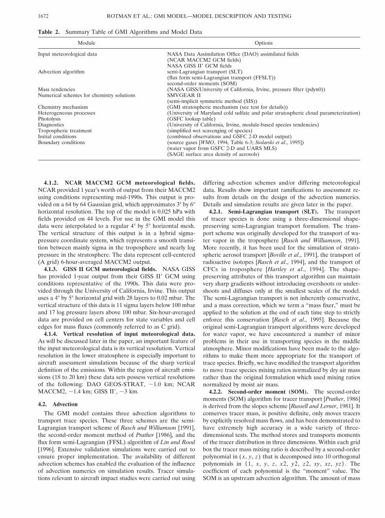
GMI assessment model, paying particular attention to thosemodules having multiple options. These modules representinput meteorological data, advection algorithms, mass tenden-cies, numerical schemes for chemistry solutions, the chemistrymechanism, heterogeneous processes, photolysis, diagnostics,treatment of tropospheric processes, and initial and boundaryconditions. Table 2 summarizes these algorithms and options

and shows those options selected for use in assessment simu-lations enclosed in parentheses.

4.1. Meteorological Input Data

The GMI model incorporates three different sets of inputmeteorological data: two from general circulation model(GCM) outputs, the National Center for Atmospheric Re-search (NCAR) Middle Atmospheric Version of the Commu-nity Climate Model, Version 2 (MACCM2) and the GoddardInstitute for Space Studies (GISS) Model II9, and one set ofGEOS-Stratospheric Tracers of Atmospheric Transport(STRAT) assimilated data representing 1996 from the NASAData Assimilation Office. Data from all these input sets in-cluded horizontal U and V winds, temperature, and surfacepressure. Below, we give details of sources for these meteoro-logical fields.

4.1.1. Data Assimilation Office (DAO) assimilated meteo-rological fields. NASA Data Assimilation Office at Goddardhas provided data sets from the GEOS-STRAT assimilationsystem. All data are 6-hour time-averaged and were an inter-polated product from the original 28 by 2.58 by 46 level DAOoutput to a 48 by 58 by 29 level. These fields represent the yearsof May 1995 through May 1996. The top of the data set is 0.1hPa. The vertical structure is 11 sigma layers below 130 hPaand 18 log pressure levels above 130 hPa. Data were providedat cell centers (commonly referred to as A grid).

Table 1. GMI Science Team Members, Institution, and Their Contribution to the GMI Model Development, Evaluation,and Applicationa

PI Co-I Institution Contribution

Brasseur Hess, Lamarque NCAR stratospheric chemistry module and analysis of influence of stratosphere-troposphere exchange to aircraft impacts

Rasch NCAR CCM2 meteorological data sets and semi-Lagrangian transport algorithmsRood Coy, Lin NASA Goddard DAO assimilated data and the flux form semi-Lagrangian transport

algorithmDouglass Kawa, Jackman NASA Goddard model evaluation against satellite, aircraft, and surface data; photolysis

lookup table; cold sulfate and polar stratospheric cloudparameterizations

Considine NASA GSFC andUniversity of Maryland

PSC parameterization

Hansen,Rind

NASA GISS NASA GISS II9 meteorological data sets

Prather University of California,Irvine

second-order moment transport algorithm; CTM model diagnostics; masstendencies diagnostics and module

Ko Weisenstein AER Corporation 2-D model simulation and analysis and aerosol surface area density fieldsfor input to assessment simulations

Pickering Allen University of Maryland NOx lightning parameterizationJacob Logan, Spivakosy Harvard University tropospheric chemistry module; tropospheric chemistry mechanism;

emission database; and ozone climatology for model evaluationPenner University of Michigan parameterization of lightning NOx, and aerosol microphysical modelGeller Yudin SUNY, Stony Brook integration of 3-D meteorological data into 2-D model framework for

analysis of transport fieldsBaughcum,

WuebblesBoeing Company and

University of Illinoishigh-speed civil transport emission scenarios and characterization

Ramaroson ONERA, France stratospheric chemistry moduleIsaksen University of Oslo ECMWF meteorological data analysisMcConnell York University York University CTM results and analysisVisconti University of L’Aquila aerosol microphysicsTennenbaum SUNY, Purchase aircraft meteorological data input toward improvement of assimilation

productsWalcek Milford SUNY, Albany convection and deposition algorithmsKinnison LLNL stratospheric chemistry module; radionuclide simulations and analysisRotman Tannahill, Bergmann,

ConnellLLNL model infrastructure and implementation of science modules

aPI, principal investigator; Co-I, co-investigator.

1671ROTMAN ET AL.: GMI MODEL—MODEL DESCRIPTION AND TESTING

4.1.2. NCAR MACCM2 GCM meteorological fields.NCAR provided 1 year’s worth of output from their MACCM2using conditions representing mid-1990s. This output is pro-vided on a 64 by 64 Gaussian grid, which approximates 38 by 68horizontal resolution. The top of the model is 0.025 hPa withfields provided on 44 levels. For use in the GMI model thisdata were interpolated to a regular 48 by 58 horizontal mesh.The vertical structure of this output is in a hybrid sigma-pressure coordinate system, which represents a smooth transi-tion between mainly sigma in the troposphere and nearly logpressure in the stratosphere. The data represent cell-centered(A grid) 6-hour-averaged MACCM2 output.

4.1.3. GISS II GCM meteorological fields. NASA GISShas provided 1-year output from their GISS II9 GCM usingconditions representative of the 1990s. This data were pro-vided through the University of California, Irvine. This outputuses a 48 by 58 horizontal grid with 28 layers to 0.02 mbar. Thevertical structure of this data is 11 sigma layers below 100 mbarand 17 log pressure layers above 100 mbar. Six-hour-averageddata are provided on cell centers for state variables and celledges for mass fluxes (commonly referred to as C grid).

4.1.4. Vertical resolution of input meteorological data.As will be discussed later in the paper, an important feature ofthe input meteorological data is its vertical resolution. Verticalresolution in the lower stratosphere is especially important toaircraft assessment simulations because of the sharp verticaldefinition of the emissions. Within the region of aircraft emis-sions (18 to 20 km) these data sets possess vertical resolutionsof the following: DAO GEOS-STRAT, ;1.0 km; NCARMACCM2, ;1.4 km; GISS II9, ;3 km.

4.2. Advection

The GMI model contains three advection algorithms totransport trace species. These three schemes are the semi-Lagrangian transport scheme of Rasch and Williamson [1991],the second-order moment method of Prather [1986], and theflux form semi-Lagrangian (FFSL) algorithm of Lin and Rood[1996]. Extensive validation simulations were carried out toensure proper implementation. The availability of differentadvection schemes has enabled the evaluation of the influenceof advection numerics on simulation results. Tracer simula-tions relevant to aircraft impact studies were carried out using

differing advection schemes and/or differing meteorologicaldata. Results show important ramifications to assessment re-sults from details on the design of the advection numerics.Details and simulation results are given later in the paper.

4.2.1. Semi-Lagrangian transport (SLT). The transportof tracer species is done using a three-dimensional shape-preserving semi-Lagrangian transport formalism. The trans-port scheme was originally developed for the transport of wa-ter vapor in the troposphere [Rasch and Williamson, 1991].More recently, it has been used for the simulation of strato-spheric aerosol transport [Boville et al., 1991], the transport ofradioactive isotopes [Rasch et al., 1994], and the transport ofCFCs in troposphere [Hartley et al., 1994]. The shape-preserving attributes of this transport algorithm can maintainvery sharp gradients without introducing overshoots or under-shoots and diffuses only at the smallest scales of the model.The semi-Lagrangian transport is not inherently conservative,and a mass correction, which we term a “mass fixer,” must beapplied to the solution at the end of each time step to strictlyenforce this conservation [Rasch et al., 1995]. Because theoriginal semi-Lagrangian transport algorithms were developedfor water vapor, we have encountered a number of minorproblems in their use in transporting species in the middleatmosphere. Minor modifications have been made to the algo-rithms to make them more appropriate for the transport oftrace species. Briefly, we have modified the transport algorithmto move trace species mixing ratios normalized by dry air massrather than the original formulation which used mixing ratiosnormalized by moist air mass.

4.2.2. Second-order moment (SOM). The second-ordermoments (SOM) algorithm for tracer transport [Prather, 1986]is derived from the slopes scheme [Russell and Lerner, 1981]. Itconserves tracer mass, is positive definite, only moves tracersby explicitly resolved mass flows, and has been demonstrated tohave extremely high accuracy in a wide variety of three-dimensional tests. The method stores and transports momentsof the tracer distribution in three dimensions. Within each gridbox the tracer mass mixing ratio is described by a second-orderpolynomial in ( x , y , z) that is decomposed into 10 orthogonalpolynomials in {1, x , y , z , x2, y2, z2, xy , xz , yz}. Thecoefficient of each polynomial is the “moment” value. TheSOM is an upstream advection algorithm. The amount of mass

Table 2. Summary Table of GMI Algorithms and Model Data

Module Options

Input meteorological data NASA Data Assimilation Office (DAO) assimilated fields(NCAR MACCM2 GCM fields)NASA GISS II9 GCM fields

Advection algorithm semi-Lagrangian transport (SLT)(flux form semi-Lagrangian transport (FFSLT))second-order moments (SOM)

Mass tendencies (NASA GISS/University of California, Irvine, pressure filter (pdyn0))Numerical schemes for chemistry solutions SMVGEAR II

(semi-implicit symmetric method (SIS))Chemistry mechanism (GMI stratospheric mechanism (see text for details))Heterogeneous processes (University of Maryland cold sulfate and polar stratospheric cloud parameterization)Photolysis (GSFC lookup table)Diagnostics (University of California, Irvine, module-based species tendencies)Tropospheric treatment (simplified wet scavenging of species)Initial conditions (combined observations and GSFC 2-D model output)Boundary conditions (source gases [WMO, 1994, Table 6-3; Stolarski et al., 1995])

(water vapor from GSFC 2-D and UARS MLS)(SAGE surface area density of aerosols)


from the upstream box is “cut off” and moved into the down-stream box where the two different polynomial distributionsare then combined (addition/conservation of moments isequivalent to least squares fitting to the polynomials). Oneadvantage of storing the tracer distribution (instead of recal-culating it each step) is that advection involves only the imme-diate upstream/downstream boxes and does not require neigh-boring points to fit polynomials. The algorithm works on thebackground “mass” of the boxes and thus has no problems withoperator splitting in flow fields where mass can accumulateduring intermediate steps. The accuracy of the method is basedin part on its storage of nine additional quantities beyond justthe mean amount of tracer. These additional memory require-ments, however, are only equivalent to doubling the resolutionin three dimensions (factor of 8) and still give better accuracy.In atmospheric modeling, the chemistry and emission patternsare often mapped onto and directly interact with the higher-order moments. The SOM scheme in its original form (1986)has the disadvantage that it generates anomalous ripples nearsharp gradients. We have included options to the originalscheme which reduce these ripples.

4.2.3. Flux form semi-Lagrangian transport (FFSLT).The third advection scheme is the flux form semi-Lagrangiantransport (FFSLT) algorithm of Lin and Rood [1996]. Thisscheme is a multidimensional algorithm that explicitly consid-ers the fluxes associated with cross terms to enable the use ofone-dimensional schemes as the basic building block. Theseone-dimensional operators are based on high-order Godunov-type finite volume schemes (primarily third-order piecewiseparabolic method (PPM)). The algorithm is upstream in na-ture to reduce phase errors and contains multiple monotonicityconstraints to eliminate the need for a filling algorithm and thesevere problems that would arise with negative values of chem-ical species concentrations. These constraints act to constrainsubgrid tracer distributions. This scheme also avoids the strictCourant stability problem at the poles, thus allowing large timesteps to be used, resulting in a highly efficient advection.

The algorithm uses two-dimensional horizontal winds frominput meteorological data to derive vertical mass fluxes fromconservation of mass and the hydrostatic continuity equation.Fluxes at the model top and surface are identically zero. Themodel can incorporate pure sigma, pure log pressure, or anycombination sigma and log pressure as vertical coordinates.

Simulation results from the NASA Models and Measure-ments II exercise [Park et al., 1999] showed this algorithm tohave an optimal combination of low diffusion, conservation,and computational performance; hence the FFSLT was se-lected for work described in this paper. Details of these sim-ulations are shown in section 6.

4.3. Mass Tendencies

In models describing the meteorological fields, that is, theclimate or assimilation models from which GMI derives itsmeteorological fields, the surface pressure varies according tothe convergence of total mass by the wind fields. In most ofthese models, however, there are discrepancies between thepressure tendency and the column convergence of mass due tomass redistribution that is not explicitly resolved by the winds(e.g., Shapiro filtering of surface pressure). Other possiblesources for these discrepancies are numerical differences be-tween the equation for the pressure tendency and the derivedmass fluxes used by chemistry models or possibly, simply, theuse of time-averaged fields where the averaging may have

impacted the close relationship between pressure tendency andcolumn convergence. When chemistry models use the meteo-rological fields, the column air mass will deviate from thesurface pressure predicted by the climate/assimilation model,and this difference, P(CTM) 2 P(met field), is designated asthe pressure error P(err). All known chemistry models havethis problem, even those running “on-line.”

A simple fix that most chemistry models adopt is merely toreset the surface pressure to that of the meteorological fieldevery 6 to 24 hours. In doing this, the air mass in the columnis abruptly changed, usually by a few tenths of a percent (i.e.,a few hPa). The chemistry model designer has the option ofconserving the tracer mass (in which case the error correctioninduces errors in the tracer mixing ratio of similar magnitude)or conserving mixing ratio (in which case the tracer mass de-velops similar magnitude errors). If the pressure errors aresmall, then the former fix is usually adopted and is not appar-ent as an error, and the induced variability is swamped by therest of the processes in the chemistry model. Nevertheless thisresetting of the surface pressure does create “source/sink-like”terms in the tracer and can induce upward/downward flowacross sigma surfaces. Since the GMI model transports speciesas volume mixing ratio, variations in the total mass of theatmosphere will necessarily yield variations in the total burdenof atmospheric chemical species. Such variations could influ-ence interpretation of simulation results.

A simple fix to the P(err) problem has been implemented inGMI. The key is to generate a resolved (u , v) wind field thatcorrects the P(err) by a resolved mass flow that carries tracerwith it, thus conserving total tracer mass and mixing ratio. Apressure filter maintains the CTM and meteorological fieldsurface pressures separately. For each new met field (e.g.,every 3 hours) the projected P(CTM) is compared with theP(met) to generate a P(err). The P(err) is then filtered togenerate a (u , v)-corrected wind field that when added to theoriginal (u , v) field, greatly reduces (but does not entirelyeliminate) P(err). (An exact Laplace solution eliminatingP(err) is possible, but not worth the computational effort.) Inthis way the P(CTM) field is different from P(met), yet followsthe P(met) field for multiyear simulations [Prather et al., 1987].

4.4. Numerical Schemes for Chemistry Solutions

4.4.1. SMVGEAR II. SMVGEAR II [Jacobson, 1995] is atechnique capable of highly accurate solutions to both stiff andnonstiff sets of ordinary differential equations. SMVGEAR IIis a version of the original predictor/corrector, backward dif-ferentiation code of Gear [1967] and uses a variable time step,variable-order, implicit technique for solving stiff numericalsystems with strict error control. The chemical continuity equa-tion is solved for each individual species (i.e., no lumping ofspecies into chemical families are made). SMVGEAR II, asdesigned for large vector supercomputers, separates the griddomain into blocks of grid cells, each containing approximately500 grid cells (large vector lengths are optimal). The cells ineach block are reordered for stiffness (see Jacobson [1995] fordetails) and solved. In GMI model simulations using massivelyparallel computers (more information on parallel computing isin following sections) we found that reducing the block sizefrom 500 to around 60–80 produced a 20% gain in speed withno loss of accuracy. With its high accuracy, SMVGEAR II wasused as a benchmark to assess the accuracy of other chemistrysolution techniques.


4.4.2. ONERA-SIS. The semi-implicit symmetric (SIS)method was developed, numerically analyzed, and applied forvarious atmospheric models by Ramaroson [1989]. It was de-veloped to include chemical tendencies in an operator splitGCM (currently, the EMERAUDE model of METEOFRANCE [Ramaroson, 1989; Ramaroson et al., 1991, 1992a,1992b; Chipperfield et al., 1993] and is also used in the MEDI-ANTE 3-D chemical transport model [Sausen et al., 1995;Claveau and Ramaroson, 1996] and box models calculations[Ramaroson et al., 1992a]. The method has also been applied tocombustion chemistry and aqueous phase within clouds. TheSIS method is more precise than explicit and implicit Eulersolutions. However, when compared to the Gear’s method(like SMVGEAR II), SIS is less precise near sunset and sun-rise only where SMVGEAR uses a higher-order expansion anda very small time step (see discussion in section 6).

4.5. Chemistry Mechanism

The GMI model includes a mechanism focused on strato-spheric chemistry with simplified tropospheric chemistry (i.e.,methane). The mechanism includes photolysis and reactions ofspecies in the species families Ox, NOy, ClOy, HOy, BrOy,CH4, and its oxidation products. The chemical mechanismincludes 46 transported species, 116 thermal reactions, and 38photolytic reactions. Source gases present in the model includeN2O, CH4, CO2, CO, the chlorine-containing compoundsCFC-11, -12, -113, -114, -115, HCFC-22, CCl4, CH3CCl3, andCH3Cl, and the bromine-containing compounds CH3Br,CF2ClBr, and CF3Br (see Table 3). Absorption cross sectioninformation was assembled from a variety of sources, includingJet Propulsion Laboratory (JPL) Publication 97-4. Most of thethermal reaction rate constants were taken from DeMore et al.[1997], the NASA Panel recommendations provided in JPLPublication 97-4.

In simulations used to compare directly to observed data,the model did include the ClO 1 OH 3 HOCl reaction;however, in assessment simulations of aircraft in 2015 thisreaction was not included. This was done to remain moreconsistent with the 2-D models which also carried out assess-ment simulations. A detailed treatment of heterogeneous pro-cesses on both sulfate and ice aerosols are included within thismechanism [Considine et al., 2000].

4.6. Heterogeneous Processes

The GMI model includes a parameterization of polar strato-spheric clouds (PSC) that will respond to increases in HNO3

and H2O produced, for example, by aircraft emissions. Bothtype 1 and type 2 PSCs are considered. The parameterizationalso accounts for PSC sedimentation, which can produce deni-trification and dehydration at the poles. The GMI PSC param-eterization is designed to be economical, so it does not repre-sent the microphysical processes governing PSC behavior.Here we describe the basics of the parameterization; moredetails on this module are given by Considine et al. [2000].

The parameterization calculates surface area densities(SAD) for type 1 and type 2 PSCs using model-calculatedtemperatures and HNO3 concentrations, aircraft emitted wa-ter vapor as well as background H2O distributions, the ambientpressure, and an H2SO4 concentration which is inferred fromthe background liquid binary sulfate (LBS) aerosol distributionspecified in the model calculation. The type 1 PSC calculationcan be set to assume either a nitric acid trihydrate (NAT) or aSTS composition (it is currently set to STS). The assumed

composition of the type 2 PSCs is water ice. The vapor pressuremeasurements of Hanson and Mauersberger [1988] are used forNAT PSCs; the approach of Carslaw et al. [1995] is used for theSTS composition; and Marti and Mauersberger [1993] vaporpressures are used for ice aerosols. The code removes bothH2O and HNO3 from gas to condensed phase when particlesform. To calculate the amount of material removed from gasphase, the parameterization assumes thermodynamic equilib-rium. When ice PSCs form, the algorithm assumes that a co-existing NAT phase also forms and is part of the type 2 PSC.This provides a mechanism for significant denitrification of thepolar stratosphere due to rapid sedimentation of the large type2 PSCs. A user-specified threshold supersaturation ratio forboth NAT and ice aerosols must be exceeded before any massis removed from the gas phase. Current values for these ratioscorrespond to a 3 K supercooling for NAT aerosols and a 2 Ksupercooling for ice aerosols, consistent with the estimates ofPeter et al. [1991] and Tabazadeh et al. [1997].

In order to calculate the surface area density correspondingto a particular amount of condensed phase mass, the codeassumes the condensed phase mass to obey a lognormal par-ticle size distribution. The user can specify either the totalparticle number density and the distribution width, or the par-ticle median radius and the distribution width, which thendetermines the conversion from condensed phase mass to sur-face area density. When the particle number density is heldconstant, condensation or evaporation processes result in thegrowth or shrinkage of existing particles rather than new par-ticle nucleation. This is thought to be more physically realistic.

The parameterization transports the condensed phase H2Oand HNO3 vertically to account for particle sedimentation.The condensed phase constituents are also subject to transportby the model wind fields. Fall velocities are calculated accord-ing to Kasten [1968] and corrected to account for the range offall velocities in a lognormally distributed ensemble of aerosolparticles. This correction factor can be important [see Consid-ine et al., 2000]. Because the GMI model currently specifies thebackground distribution of H2O in the stratosphere, a specialstrategy had to be developed to allow for dehydration resultingfrom particles sedimentation. This takes the form of a specialtransported constituent (named “dehyd”) which is producedwhen dehydration occurs due to particle sedimentation and islost when moistening of a region results from local evaporationof particles sedimenting from higher altitudes. Ambient H2Oconcentrations are then the difference between the back-ground H2O and “dehyd.”

It should be stressed that this parameterization is not mi-crophysical. A comprehensive microphysical representation ofPSCs would be computationally expensive and so is not appro-priate in a model designed for assessment calculations.

4.7. Photolysis

Photolysis rates are obtained by a clear-sky lookup table[Douglass et al., 1997]. Normalized radiative fluxes calculatedfrom the model of Anderson et al. [1995] are tabulated as afunction of wavelength, solar zenith angle, overhead ozone,and pressure. Temperature-dependent molecular cross sec-tions, quantum yields, and solar flux are tabulated separately.In the GMI model, fluxes and cross sections are interpolated tothe appropriate values for each grid and integrated over wave-length to produce photolysis rates. This method compares wellto the photolysis benchmark intercomparisons [Stolarski et al.,1995]. Photolysis rates are obtained using a uniform global


Table 3. Detailed Description of the GMI Chemical Mechanism, Reactions, and Rates

Kinetic Parameters Notes

A E/R a

k0300 n k`

300 m B b

ReactionsO 1 O2 1 M 5 O3 6.0e-34 2. 0. 0. c

3.O 1 O3 5 2 O2 8.0e-12 2060. cO(1D) 1 N2 5 O 1 N2 1.8e-11 2110. cO(1D) 1 O2 5 O 1 O2 3.2e-11 270. cO(1D) 1 O3 5 2 O2 1.2e-10 0. cO(1D) 1 H2O 5 2 OH 2.2e-10 0. cO(1D) 1 H2 5 OH 1 H 1.1e-10 0. cO(1D) 1 N2O 5 N2 1 O2 4.9e-11 0. cO(1D) 1 N2O 5 2 NO 6.7e-11 0. cO(1D) 1 CH4 5 CH3O2 1 OH 1.125e-10 0. cO(1D) 1 CH4 5 CH2O 1 H 1 HO2 3.0e-11 0. cO(1D) 1 CH4 5 CH2O 1 H2 7.5e-12 0. c (branching ratio, JPL note A9)O(1D) 1 CF2Cl2 5 2 Cl 1.20e-10 0. c (JPL notes A2 and A15)O(1D) 1 CFC113 5 3 Cl 1.50e-10 0. c (JPL note A15)O(1D) 1 HCFC22 5 Cl 7.20e-11 0. c (JPL notes A15 and A23)H 1 O2 1 M 5 HO2 5.7e-32 1.6 7.5e-11 0. cH 1 O3 5 OH 1 O2 1.4e-10 470. cH2 1 OH 5 H2O 1 H 5.5e-12 2000. cOH 1 O3 5 HO2 1 O2 1.6e-12 940. cOH 1 O 5 O2 1 H 2.2e-11 2120. cOH 1 OH 5 H2O 1 O 4.2e-12 240. cHO2 1 O 5 OH 1 O2 3.0e-11 2200. cHO2 1 O3 5 OH 1 2 O2 1.1e-14 500. cHO2 1 H 5 2 OH 7.0e-11 0. c (products, JPL note B5)HO2 1 OH 5 H2O 1 O2 4.8e-11 2250. cHO2 1 HO2 5 H2O2 1 O2 dHO2 1 HO2 1 H2O 5 H2O2 1 O2 1 H2O eH2O2 1 OH 5 H2O 1 HO2 2.9e-12 160. cN 1 O2 5 NO 1 O 1.5e-11 3600. cN 1 NO 5 N2 1 O 2.1e-11 2100. cNO 1 O3 5 NO2 1 O2 2.0e-12 1400. cNO2 1 OH 1 M 5 HNO3 2.32e-30 2.97 1.45e-11 2.77 fNO 1 HO2 5 NO2 1 OH 3.5e-12 2250. cNO2 1 O 5 NO 1 O2 5.26e-12 2209. gNO2 1 O3 5 NO3 1 O2 1.2e-13 2450. cNO2 1 HO2 1 M 5 HO2NO2 1.8e-31 3.2 4.7e-12 1.4 cNO3 1 O 5 O2 1 NO2 1.0e-11 0. cNO3 1 NO 5 2 NO2 1.5e-11 2170. cNO3 1 NO2 1 M 5 N2O5 2.2e-30 3.9 1.5e-12 0.7 cN2O5 1 M 5 NO2 1 NO3 8.15e-04 3.9 5.56e114 0.7 11000. cHNO3 1 OH 5 H2O 1 NO3 c (see expression in reference)HO2NO2 1 M 5 HO2 1 NO2 8.57e-05 3.2 2.24e115 1.4 10900. cHO2NO2 1 OH 5 H2O 1 NO2 1 O2 1.3e-12 2380. c (products assumed)Cl 1 O3 5 ClO 1 O2 2.9e-11 260. cCl 1 H2 5 HCl 1 H 3.7e-11 2300. cCl 1 H2O2 5 HCl 1 HO2 1.1e-11 980. cCl 1 HO2 5 HCl 1 O2 1.8e-11 2170. cCl 1 HO2 5 OH 1 ClO 4.1e-11 450. cClO 1 O 5 Cl 1 O2 3.0e-11 270.0 cClO 1 OH 5 HO2 1 Cl 1.1e-11 2120. k from c, see h for branching ratioClO 1 OH 5 HCl 1 O2 1.1e-11 2120. k from c, see h for branching ratioClO 1 HO2 5 O2 1 HOCl 4.8e-13 2700. c (branching ratio, JPL note F43)ClO 1 HO2 5 O3 1 HCl 0.0e-00 0. c (branching ratio, JPL note F43)ClO 1 NO 5 NO2 1 Cl 6.4e-12 2290. cClO 1 NO2 1 M 5 ClONO2 1.8e-31 3.4 1.5e-11 1.9 cClO 1 ClO 5 2 Cl 1 O2 3.0e-11 2450. cClO 1 ClO 5 Cl2 1 O2 1.0e-12 1590. cClO 1 ClO 5 Cl 1 OClO 3.5e-13 1370. cClO 1 ClO 1 M 5 Cl2O2 2.2e-32 3.1 3.5e-12 1.0 cCl2O2 1 M 5 2 ClO 1.69e-05 3.1 2.69e115 1.0 8744. cHCl 1 OH 5 H2O 1 Cl 2.6e-12 350 cHOCl 1 OH 5 H2O 1 ClO 3.0e-12 500. cClONO2 1 O 5 ClO 1 NO3 4.5e-12 900. iClONO2 1 OH 5 HOCl 1 NO3 1.2e-12 330. c (products assumed)ClONO2 1 Cl 5 Cl2 1 NO3 6.5e-12 2135. c (products, JPL note F71)Br 1 O3 5 BrO 1 O2 1.7e-11 800. cBr 1 HO2 5 HBr 1 O2 1.5e-11 600. c


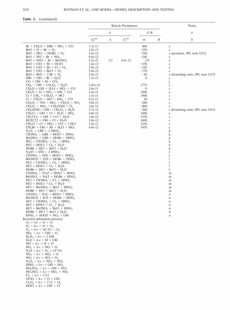
Table 3. (continued)


A E/R a

k0300 n k`

300 m B b

Br 1 CH2O 5 HBr 1 HO2 1 CO 1.7e-11 800. cBrO 1 O 5 Br 1 O2 1.9e-11 2230. cBrO 1 HO2 5 HOBr 1 O2 3.4e-12 2540. c (products, JPL note G21)BrO 1 NO 5 Br 1 NO2 8.8e-12 2260. cBrO 1 NO2 1 M 5 BrONO2 5.2e-31 3.2 6.9e-12 2.9 cBrO 1 ClO 5 Br 1 OClO 1.6e-12 2430. cBrO 1 ClO 5 Br 1 Cl 1 O2 2.9e-12 2220. cBrO 1 ClO 5 BrCl 1 O2 5.8e-13 2170. cBrO 1 BrO 5 2 Br 1 O2 2.4e-12 240. c (branching ratio, JPL note G37)HBr 1 OH 5 Br 1 H2O 1.1e-11 0 cCO 1 OH 5 H 1 CO2 jCH4 1 OH 5 CH3O2 1 H2O 2.45e-12 1775. cCH2O 1 OH 5 H2O 1 HO2 1 CO 1.0e-11 0. cCH2O 1 O 5 HO2 1 OH 1 CO 3.4e-11 1600. cCl 1 CH4 5 CH3O2 1 HCl 1.1e-11 1400. cCl 1 CH2O 5 HCl 1 HO2 1 CO 8.1e-11 30. cCH3O2 1 NO 5 HO2 1 CH2O 1 NO2 3.0e-12 2280. cCH3O2 1 HO2 5 CH3OOH 1 O2 3.8e-13 2800. cCH3OOH 1 OH 5 CH3O2 1 H2O 2.7e-12 2200. c (branching ratio, JPL note D15)CH3Cl 1 OH 5 Cl 1 H2O 1 HO2 4.0e-12 1400. cCH3CCl3 1 OH 5 3 Cl 1 H2O 1.8e-12 1550. cHCFC22 1 OH 5 Cl 1 H2O 1.0e-12 1600. cCH3Cl 1 Cl 5 HO2 1 CO 1 2 HCl 3.2e-11 1250. cCH3Br 1 OH 5 Br 1 H2O 1 HO2 4.0e-12 1470. cN2O5 1 LBS 5 2 HNO3 kClONO2 1 LBS 5 HOCl 1 HNO3 kBrONO2 1 LBS 5 HOBr 1 HNO3 kHCl 1 ClONO2 5 Cl2 1 HNO3 kHCl 1 HOCl 5 Cl2 1 H2O kHOBr 1 HCl 5 BrCl 1 H2O kN2O5 1 STS 5 2 HNO3 lClONO2 1 STS 5 HOCl 1 HNO3 lBrONO2 1 STS 5 HOBr 1 HNO3 lHCl 1 ClONO2 5 Cl2 1 HNO3 lHCl 1 HOCl 5 Cl2 1 H2O lHOBr 1 HCl 5 BrCl 1 H2O lClONO2 1 NAT 5 HOCl 1 HNO3 mBrONO2 1 NAT 5 HOBr 1 HNO3 mHCl 1 ClONO2 5 Cl2 1 HNO3 mHCl 1 HOCl 5 Cl2 1 H2O mHCl 1 BrONO2 5 BrCl 1 HNO3 mHOBr 1 HCl 5 BrCl 1 H2O mClONO2 1 ICE 5 HOCl 1 HNO3 nBrONO2 1 ICE 5 HOBr 1 HNO3 nHCl 1 ClONO2 5 Cl2 1 HNO3 nHCl 1 HOCl 5 Cl2 1 H2O nHCl 1 BrONO2 5 BrCl 1 HNO3 nHOBr 1 HCl 5 BrCl 1 H2O nHNO3 1 SOOT 5 NO2 1 OH o

Reaction (photolysis process)O2 1 hn 5 O 1 OO3 1 hn 5 O 1 O2O3 1 hn 5 O(1D) 1 O2HO2 1 hn 5 OH 1 OH2O2 1 hn 5 2 OHH2O 1 hn 5 H 1 OHNO 1 hn 5 N 1 ONO2 1 hn 5 NO 1 ON2O 1 hn 5 N2 1 O(1D)NO3 1 hn 5 NO2 1 ONO3 1 hn 5 NO 1 O2N2O5 1 hn 5 NO2 1 NO3HNO3 1 hn 5 OH 1 NO2HO2NO2 1 hn 5 OH 1 NO3HO2NO2 1 hn 5 HO2 1 NO2Cl2 1 hn 5 2 ClOClO 1 hn 5 O 1 ClOCl2O2 1 hn 5 2 Cl 1 O2HOCl 1 hn 5 OH 1 Cl


mean surface albedo of 0.3 and a cloud-free atmosphere. Crosssections and quantum yields are from DeMore et al. [1997].

4.8. Diagnostics

Diagnostics have been implemented in the GMI model toenable assessing total mass and the changes in species concen-trations in each grid box caused by each operator (i.e., hori-zontal and vertical advection, chemistry, etc.). The diagnostictracks concentrations before and after each module, and pro-vides time-averaged information in one-dimensional (in alti-tude) or two-dimensional (in latitude and altitude) output.Such diagnostics are very useful in analyzing what processescontrol the distribution of chemical species in particular re-gions of the atmosphere.

4.9. Tropospheric Treatment and Transport

The chemical mechanism was focused primarily on qualityand efficient stratospheric chemistry simulations. For wet scav-enging, the model used a simple vertically dependent removallifetime [Logan, 1983]. Near the ground the lifetime of wet-deposited species was assumed to be 1 day and increases to 38days near the tropopause. Species deposited using this methodare HNO3, HCl, and BrONO2. There are no surface emissionsof chemical species, and the model does not include dry dep-

osition, vertical diffusion, or convection schemes for tracertransport.

4.10. Initial and Boundary Conditions

Zonally averaged initial conditions for chemical species areobtained from the GSFC 2-D model. Boundary conditions forthe source gases in the GSFC 2-D model were set as follows:evaluation/validation runs for comparison to observations used1995 conditions from WMO [1994, Table 6-3], while aircraftassessment simulations representing 2015 used conditions de-scribed by Stolarski et al. [1995]. For these long-lived speciesthe GMI model reset the bottom two model layers to thevalues obtained from initial conditions.

The GMI focused on stratospheric chemical processes im-portant to HSCT assessments and did not attempt to predictthe background distribution of water vapor related to complextropospheric hydrologic processes. Instead, it incorporated wa-ter vapor fields obtained from an assimilation of MLS watervapor measurements into the GSFC 2-D model. To allow thepolar stratospheric cloud parameterization to correctly repre-sent polar processes such as dehydration, the background wa-ter vapor fields necessarily eliminated any dehydration as seenin MLS measurements. A regression algorithm involvingCLAES N2O measurements and MLS water vapor measure-

Table 3. (continued)


A E/R a

k0300 n k`

300 m B b

Reaction (photolysis process)ClONO2 1 hn 5 Cl 1 NO3ClONO2 1 hn 5 ClO 1 NO2BrCl 1 hn 5 Br 1 ClBrO 1 hn 5 Br 1 OHOBr 1 hn 5 Br 1 OHBrONO2 1 hn 5 Br 1 NO3BrONO2 1 hn 5 BrO 1 NO2CH3OOH 1 hn 5 CH2O 1 HO2 1 OHCH2O 1 hn 5 CO 1 H2CH2O 1 hn 5 HO2 1 CO 1 HCH3Cl 1 hn 5 CH3O2 1 ClCCl4 1 hn 5 4 ClCH3CCl3 1 hn 5 3 ClCFCl3 1 hn 5 3 ClCF2Cl2 1 hn 5 2 ClCFC113 1 hn 5 3 ClCH3Br 1 hn 5 Br 1 CH3O2CF3Br 1 hn 5 BrCF2ClBr 1 hn 5 Br 1 Cl

ak 5 Ae2E/RT.bk 5 {(k0(T)[M])/(1 1 k0(T)[M]/k`(T))}0.6{11[log10(k0(T)[M]/k`(T))]2}21

e2B/T, k0(T) 5 k0300(T/300)2n, k`(T) 5 k`

300(T/300)2m.cDeMore et al. [1997].dk 5 2.3 3 10213e600/T 1 1.7 3 10233[M]e1000/T.ek 5 (2.3 3 10213e600/T 1 1.7 3 10233[M]e1000/T)1.4 3 10221e2200/T.fBrown et al. [1999].gGierczak et al. [1999].hLipson et al. [1997]; branching ratio for HCl as product 5 1.7 3 10213e363/T/4.2 3 10212e280/T.iGoldfarb et al. [1998].jFrom reference in note c above; k 5 1.5 3 10213(1.0 1 0.6P), P in atm.kHeterogeneous surface reaction; LBS represents liquid binary sulfate aerosol surface area.lHeterogeneous surface reaction; STS represents sulfate ternary solution aerosol surface area (PSC type I).mHeterogeneous surface reaction; NAT represents nitric acid trihydrate aerosol surface area (alternate form of PSC type I).nHeterogeneous surface reaction; ICE represents ice aerosol surface area (PSC type II).oHeterogeneous surface reaction; SOOT represents carbonaceous aerosol surface area.


ments was used to fill dehydrated regions in the MLS obser-vations. The resulting altered MLS water vapor distribution(from 808S to 808N, and from 70 hPa to 0.3 hPa) was used toconstrain the GSFC 2-D model. In the troposphere, watervapor was further constrained by observations of Oort [1983].Steady state 2-D water vapor fields were used as background inGMI simulations.

The GMI model used distributions of monthly averagedaerosol surface area densities for heterogeneous reactions onsulfate aerosols. For present-day simulations of the GMImodel, we used SAGE-based surface area density data fromThomason et al. [1997] which described the background distri-bution of aerosols during the year of 1996. For the aircraftassessment we used the designated SA0 distribution represent-ing a clean atmosphere as detailed by WMO [1992, Table 8-8].In neither case did we attempt to include the sulfate aerosolscreated by the combustion process of aircraft fuels containingsulfur. Two-dimensional model simulations of aircraft effectsshow important perturbations caused by this additional sourceof sulfate aerosols [Kawa et al., 1999; IPCC, 1999]. Future workwith the GMI model will include these effects.

5. Parallelization and ComputationalTimings of GMI

Three-dimensional atmospheric chemistry models requirelarge amounts of computer time and effort because of thecomplex nature of the modeling and the need to perform longsimulations due to the long timescales of the stratosphere. Toenable multiyear chemistry simulations, the GMI core modelwas parallelized to make use of the most powerful computa-tional platforms available. An existing LLNL computationalframework [Mirin et al., 1994] was used to implement the GMImodel on parallel computers. This framework uses a two-dimensional longitude/latitude domain decompositionwhereby each subdomain consists of a number of contiguouscolumns having a full vertical extent. Processors are assigned tosubdomains, and variables local to a given package/subdomainare stored on the memory of the assigned processor. Data aretransmitted between computational processes, when needed,in the form of messages. The number of meshpoints per sub-domain may be nonuniform, under the constraint that thedecomposition be logically rectangular. The choice to decom-pose in only two dimensions is based on the fact that thechemistry, photolysis, and cold sulfate algorithms make up thevast majority of the computational requirements and are alleither local or column calculations. Thus these computationsrequire no communication with neighboring grid zones andhence maximize the parallel efficiency.

Because of the wide spectrum of architectures together witha typical computer lifetime of just a few years, it is importantto maintain a portable source code. We have encountered twomajor issues that affect portability: message passing and dy-namic memory management. To address these issues, we usethe MPI message passing interface and FORTRAN90’s dy-namic memory capabilities. The GMI model runs on virtuallyall leading edge massively parallel processors, including theCray-T3E, SGI Origin2000, and IBM-SP. The model also runson clusters of workstations (IBM, SUN, COMPAQ/DEC), aswell as on the Cray-C90 and J90 (multitasking was not imple-mented in the model, hence C90 and J90 simulations used oneprocessor). Although portability is quite important, it is equally

important to exploit each architecture as much as possible.Toward that end, the framework makes use of conditionalcompilation to allow inclusion of optimization constructs par-ticular to given architectures. The parallel framework providesthe domain decomposition functionality, the detailed aspectsof the message passing, and a number of other useful utilities.Nearly all coding in the model is written in FORTRAN 77/90,with a small amount of C. This framework is the backbone ofthe GMI model. All submitted algorithms and modules havebeen incorporated into this structure. This two-dimensionaldecomposition does impose communication requirements inthe east-west and north-south advection operator. The FFSLTscheme requires species information in the adjacent two cellsin order to form the profiles of species distributions to establishthe flux of species through cell edges. However, the uniquecapability of the FFSLT to accurately deal with high Courantnumber flows in the east-west direction near the poles was aspecial issue for parallelization. In that region of the grid thesize of the grid zone becomes very small in the east-westdirection, and to enable large time steps (i.e., Courant stabilitydefined on the equatorial grid sizes), the Courant numbersnear the pole become larger than 1. The algorithm accuratelydeals with these large Courant numbers in the polar region bychanging its advection algorithm to one that possesses a La-grangian (trajectory) character (here it shares many character-istics with traditional semi-Lagrangian methods, and hence itsname of the flux form semi-Lagrangian scheme; see Lin andRood [1996] for details of the implementation). With the pos-sibility of Courant numbers much larger than one, we neededto ensure domains have species information at locations largerthan two adjacent grid zones. For each subdomain we maintain“ghost cells” which represents the species information in theadjacent zones. Information in these ghost zones is exchangedbetween domains via message passing. The possibility of largeCourant numbers in the polar regions forces the need for largenumbers of ghost zones in the east-west direction, which in-creases the communication cost (and hence, decreases theparallel efficiency). As a compromise, we use four ghost zonesin each direction and adjust the time step to ensure Courantnumbers are never larger than four.

The parallelization effort has worked well to allow multiyearstratospheric chemistry simulations and has enabled the appli-cation of the GMI model to the assessment of stratosphericaircraft emissions [Kawa et al., 1999; Kinnison et al., this issue].The breakdown of the CPU requirements on a Cray C90 forthe GMI model is as follows: chemistry, 78%; advection, 12%;photolysis, 7%; cold sulfate/PSC, 3%. These values are approx-imate only and represent the breakdown on a C90 style largevector machine (see next section for more details). Given thecommunication costs of the advection scheme, on parallel ma-chines the fraction of time spent there will be larger. However,in general, the local and column processes of chemistry, pho-tolysis, and PSC/cold sulfate correspond to the majority of thecomputational needs and allow good parallel efficiency. Scal-ing is near linear when increasing processor numbers to about100. Increasing above that level, we see about 70–80% effi-ciency. This makes sense since on a given problem, increasingthe processor count decreases the number of grid zones in adomain, but the number of ghost zones required remains atfour. Eventually, you reach a point where the number of ghostzones is larger than the number of zones in the computationaldomain, which acts to decrease the parallel efficiency. None-theless, the use of parallel computers allowed us to carry out


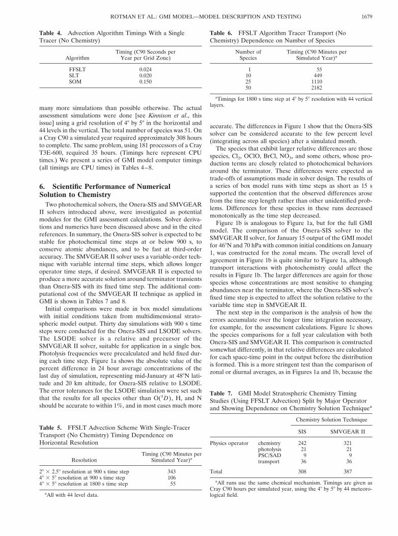
many more simulations than possible otherwise. The actualassessment simulations were done [see Kinnison et al., thisissue] using a grid resolution of 48 by 58 in the horizontal and44 levels in the vertical. The total number of species was 51. Ona Cray C90 a simulated year required approximately 308 hoursto complete. The same problem, using 181 processors of a CrayT3E-600, required 35 hours. (Timings here represent CPUtimes.) We present a series of GMI model computer timings(all timings are CPU times) in Tables 4–8.

6. Scientific Performance of NumericalSolution to Chemistry

Two photochemical solvers, the Onera-SIS and SMVGEARII solvers introduced above, were investigated as potentialmodules for the GMI assessment calculations. Solver deriva-tions and numerics have been discussed above and in the citedreferences. In summary, the Onera-SIS solver is expected to bestable for photochemical time steps at or below 900 s, toconserve atomic abundances, and to be fast at third-orderaccuracy. The SMVGEAR II solver uses a variable-order tech-nique with variable internal time steps, which allows longeroperator time steps, if desired. SMVGEAR II is expected toproduce a more accurate solution around terminator transientsthan Onera-SIS with its fixed time step. The additional com-putational cost of the SMVGEAR II technique as applied inGMI is shown in Tables 7 and 8.

Initial comparisons were made in box model simulationswith initial conditions taken from multidimensional strato-spheric model output. Thirty day simulations with 900 s timesteps were conducted for the Onera-SIS and LSODE solvers.The LSODE solver is a relative and precursor of theSMVGEAR II solver, suitable for application in a single box.Photolysis frequencies were precalculated and held fixed dur-ing each time step. Figure 1a shows the absolute value of thepercent difference in 24 hour average concentrations of thelast day of simulation, representing mid-January at 488N lati-tude and 20 km altitude, for Onera-SIS relative to LSODE.The error tolerances for the LSODE simulation were set suchthat the results for all species other than O(1D), H, and Nshould be accurate to within 1%, and in most cases much more

accurate. The differences in Figure 1 show that the Onera-SISsolver can be considered accurate to the few percent level(integrating across all species) after a simulated month.

The species that exhibit larger relative differences are thosespecies, Cl2, OClO, BrCl, NO3, and some others, whose pro-duction terms are closely related to photochemical behaviorsaround the terminator. These differences were expected astrade-offs of assumptions made in solver design. The results ofa series of box model runs with time steps as short as 15 ssupported the contention that the observed differences arosefrom the time step length rather than other unidentified prob-lems. Differences for these species in these runs decreasedmonotonically as the time step decreased.

Figure 1b is analogous to Figure 1a, but for the full GMImodel. The comparison of the Onera-SIS solver to theSMVGEAR II solver, for January 15 output of the GMI modelfor 468N and 70 hPa with common initial conditions on January1, was constructed for the zonal means. The overall level ofagreement in Figure 1b is quite similar to Figure 1a, althoughtransport interactions with photochemistry could affect theresults in Figure 1b. The larger differences are again for thosespecies whose concentrations are most sensitive to changingabundances near the terminator, where the Onera-SIS solver’sfixed time step is expected to affect the solution relative to thevariable time step in SMVGEAR II.

The next step in the comparison is the analysis of how theerrors accumulate over the longer time integration necessary,for example, for the assessment calculations. Figure 1c showsthe species comparisons for a full year calculation with bothOnera-SIS and SMVGEAR II. This comparison is constructedsomewhat differently, in that relative differences are calculatedfor each space-time point in the output before the distributionis formed. This is a more stringent test than the comparison ofzonal or diurnal averages, as in Figures 1a and 1b, because the

Table 5. FFSLT Advection Scheme With Single-TracerTransport (No Chemistry) Timing Dependence onHorizontal Resolution

ResolutionTiming (C90 Minutes per

Simulated Year)a

28 3 2.58 resolution at 900 s time step 34348 3 58 resolution at 900 s time step 10648 3 58 resolution at 1800 s time step 55

aAll with 44 level data.

Table 6. FFSLT Algorithm Tracer Transport (NoChemistry) Dependence on Number of Species

Number ofSpecies

Timing (C90 Minutes perSimulated Year)a

1 5510 44925 111050 2182

aTimings for 1800 s time step at 48 by 58 resolution with 44 verticallayers.

Table 7. GMI Model Stratospheric Chemistry TimingStudies (Using FFSLT Advection) Split by Major Operatorand Showing Dependence on Chemistry Solution Techniquea

Chemistry Solution Technique

SIS SMVGEAR II

Physics operator chemistry 242 321photolysis 21 21PSC/SAD 9 9transport 36 36

Total 308 387

aAll runs use the same chemical mechanism. Timings are given asCray C90 hours per simulated year, using the 48 by 58 by 44 meteoro-logical field.

Table 4. Advection Algorithm Timings With a SingleTracer (No Chemistry)

AlgorithmTiming (C90 Seconds per

Year per Grid Zone)

FFSLT 0.024SLT 0.020SOM 0.150


contribution of differences is not made relative to the constit-uent concentration. That is, a large relative difference encoun-tered at some point in the stratosphere where the species isvery small is given the same weight as a relative difference atthe species’ maximum abundance. The region of comparisonwas restricted to the stratosphere, and very small concentra-tions (less than 1024 molecules cm23 or a mole fraction of10224, as appropriate) were excluded. The distribution wasalso area-normalized, but not weighted for altitude or ambientpressure. The open section of the bar represents the mean ofthe distribution for each species, and the hatched bar repre-sents the relative difference value that includes 90% of thepoints in space and time. For HCl these values are actuallyinverted, in that the ninetieth percentile is less than the meanvalue, indicating a long tail on the distribution. This did notoccur for any other species.

The results of this comparison (Figure 1c) show that differ-ences accumulate slowly, an indication that the abundances of

the trace species are buffered, by the photochemical environ-ment, against transport-driven divergence of the solution. Thegrouping of species by solver difference and the magnitudes ofthe differences are similar to the results of the shorter runs inFigures 1a and 1b. This lends additional support to the choiceof Onera-SIS for the assessment runs.

Finally, consideration of the distribution and the pattern ofdifferences for each individual species can reveal whether thebehavior can be explained by the nature of the mechanism andthe expected effects of solver assumptions, or appears to signalsome error in the solver. Figure 2 shows the solver differencedistribution for ozone, plotted against the cumulative concen-tration distribution.

Ozone concentration as number density spreads over nearly2 orders of magnitude, and the mean absolute difference be-tween solvers is always less than 0.5%. At the locations of theupper 95% of ozone concentrations, 90% of the solver differ-ences are within 1%. At the locations of the upper 50% ofozone concentrations, 99% of the solver comparisons arewithin 1%. The far outliers in the difference distribution tendto occur in the south polar spring, where heterogeneous pro-cesses are activating inorganic chlorine.

The case of ozone shows that distributions of differences,summarized in Figure 1 above, are not themselves evenly dis-tributed in time and space. Differences in species with fastphotochemical time constants tend to cluster around the ter-minator. The chemical relationship of species will cause dif-ferences in one species, for example, HO2, to propagate toanother, H2O2 in this case.

For most of the species with the largest average differences,solver differences for locations with concentrations in the up-per decade (representing a few percent of the distribution) are

Figure 1. (a) Absolute value of the relative difference of the diel averages of the Onera-SIS solver relativeto the LSODE solver for 488N, 20 km, January 15, thirtieth day of repeating diel box model integration; (b)comparison of January 15 zonal mean at 468N, 70 hPa for Onera-SIS in the GMI model to SMVGEAR II inthe GMI model; (c) global, annual comparison of Onera-SIS to SMVGEAR II (see text for details).

Table 8. GMI Model Stratospheric Chemistry TimingStudies Using the FFSLT Advection, Showing Dependenceon Chemistry Solution Technique on the Cray T3E-600 andSGI Origin 2000 Platformsa

CrayT3E-600

SGIOrigin 2000

Chemistry solutiontechnique

SIS 116 103SMVGEAR II 334 163

aAll runs use the same chemical mechanism and involve all themodules needed for aircraft assessment. Timings are given as CPUhours per simulated year using 31 processors and the 48 by 58 by 44meteorological field.


much smaller than the mean. For example, Cl2 differences forthe upper decade of concentration average about 8%, withdifferences of about 2% for the largest concentrations. Re-gions of heterogeneous activation of inorganic chlorine arealso characterized by larger differences. For CH3O2, solverdifferences actually increase with number density in the cumu-lative distribution, as the largest concentrations are reachedwhen atomic Cl is large, in the austral polar spring, as a resultof the Cl 1 CH4 reaction, which is usually of lesser importance.

It is, perhaps, important to note that the solver differencesshown in the figures above are, in almost every case, not visiblecomparing the solvers side by side on the conventional contouror false color plot. The decision to select Onera-SIS for theGMI assessment calculations was made qualitatively on a cost-benefit basis, trading computational performance against ac-curacy of the photochemical species abundances, in the light ofthe necessity to complete a set of assessment runs.

7. Transport Model Application and ValidationAs discussed earlier, the GMI model incorporated the flux

form semi-Lagrangian scheme as its primary transport opera-tor. We have validated the meteorological data and transportmodel implementation through simulations of stratospherictracers and comparisons to similar model runs at the originat-ing organization. Three test cases provided the primary com-parison: a steady state N2O simulation, the NASA Models andMeasurements II [Park et al., 1999] Age of the Air diagnostic(MMII A1), and the NASA Models and Measurements IIArtificial NOx type tracer (MMII A3).

This validation took place in two stages. After implementingthe transport algorithms and meteorological data into the GMImodel, the first stage used N2O simulations to test the imple-

mentation of the advection operator and the meteorologicaldata. Using tabulated values of monthly averaged loss rates(from photolysis and O1D loss (M. Prather, personal commu-nication, 1995)), we tested these models against simulations ofN2O made using the parent models from which the GMI ad-vection schemes were taken. In each case, we were able tomatch the simulations very well indicating that the advectionschemes and meteorological data sets were correctly imple-mented. The second, and more interesting stage, was to eval-uate the application of the FFSLT algorithm to the threemeteorological data sets. For this evaluation, in addition toN2O, we also used the NASA Models and Measurements II A1and A3 tracers. The A1 tracer was a diagnostic to generate theage spectrum of the atmospheric model. The A3 tracer was theemissions of a hypothetical tracer from a projected fleet ofhigh-speed civil transports (HSCTs). For more information onthe NASA MMII tracer and analysis, see Park et al. [1999]. Thegoal was to compare the long-lived tracer distributions ob-tained using FFSLT to those distributions obtained using theparent model’s advection scheme. Thus, in stage one, we ranthe NCAR meteorological data through the NCAR SLT rou-tine and reproduced the correct profiles. Next we used theNCAR meteorological data through the FFSLT advection rou-tine to investigate differences in the profiles caused by thedifferent advection operator.

Figure 3a shows the N2O zonal averaged (steady state) pro-files from the MACCM2 meteorological data and the NCARSLT algorithm. Figure 3b shows the same calculation using theFFSLT advection operator. Comparing Figures 3a and 3bshows the profiles of N2O to be very faithfully reproducedusing the FFSLT advection operator. In its current form theFFSLT routine requires grids with equally spaced grids in the

Figure 2. The cumulative probability distribution for ozone concentration in the GMI model is shown in theupward trending solid line and is associated with the right axis. The downward trending solid line is the meanof the absolute values of the solver differences for all points with ozone concentrations larger than theindicated concentration, that is, the fiftieth percentile of the difference distribution for concentrations at orabove the threshold value. The dashed line is the ninetieth percentile difference value, for which 90% of thedifferences are smaller than the plotted value for all points with equal or greater ozone concentrations. Thedotted line is the 99th percentile.


Figure 3. Steady state zonal averaged N2O simulation results for January using the GMI model. (a) Resultsobtained using the NCAR MACCM2 meteorological input data with the semi-Lagrangian advection algo-rithm. (b) Results obtained using the NCAR MACCM2 meteorological input data with the flux formsemi-Lagrangian advection scheme. Units are ppbv.


latitude and longitude direction. Since the MACCM3 datawere originally provided on a Gaussian grid, the data wereinterpolated onto a fixed 48 by 58 grid. Even with this additionalinterpolation, the results match very well. The NCAR SLTroutine appears to be slightly better in keeping a strongergradient in the extratropical regions, but it is not clear whetherthis is an advection scheme issue or an issue arising from theadded interpolation.

Figure 4a shows the N2O zonal averaged (steady state) pro-file from the GISS II meteorological data and the UCI second-order moment (SOM) advection scheme. Figure 4b shows theprofile from the GISS II data obtained using the FFSLTscheme. Comparisons of these plots show the SOM is betterable to maintain gradients in the N2O profiles, but the overallstructure is reproduced very well.

It should be noted that in both of these cases, the FFSLTscheme is calculating the vertical fluxes from the input hori-zontal wind data. We have assessed the predicted vertical massfluxes in the FFSLT and in the other advection routines, and in

both cases, the FFSLT has accurately calculated the samevertical fluxes that the SLT and SOM predict when using thosemeteorological data. This validation and sensitivity test sug-gests that for long-lived tracers, like N2O, the particular char-acteristics of the advection operator do not influence the dis-tribution. This does not address whether the N2O simulationsreproduce observed data. That has been addressed by Douglasset al. [1999].

Another test of the sensitivity of stratospheric transport toadvection operator is the age diagnostic as defined by theNASA Models and Measurements II workshop (see Park et al.[1999] for details). In short, this test case inputs a short (monthlong) pulse of tracer into the equatorial lower troposphere,then stops the pulse and imposes a loss rate in the troposphere.The speed at which the tracer is eliminated from the tropo-sphere by dynamics of the stratosphere through stratosphere/troposphere exchange is representative of the residence timeand overturning rate of the stratosphere. Figures 5a and 5bshow the mean age of the MACCM2 meteorological data as

Figure 4. Steady state zonal averaged N2O simulation results for January using the GMI model. (a) Resultsobtained using the GISS II9 meteorological input data with the second-order moment method advectionscheme. (b) Results obtained using the GISS II9 meteorological input data with the flux form semi-Lagrangianadvection scheme. Units are ppbv.


simulated using the SLT and FFSLT (respectively) and Figures6a and 6b show the same using the GISS data. Again, the GMImodel results match the original model results very well. Itshould be noted that observations suggest stratospheric airwith a mean age that is longer than simulated with eitherMACCM2 or GISS II [see Hall et al., 1999]. As noted in theNASA MMII report [Park et al., 1999] and by Hall et al. [1999],this is characteristic of most two- and three-dimensional atmo-spheric models and is still an area of intense research.

The GMI model was developed to produce assessments ofthe environmental consequences from the emissions of a pro-posed fleet of supersonic aircraft. The NASA Models andMeasurements II constructed a test problem, the A3 tracertest, to evaluate the ability of a model to simulate a tracerrepresenting aircraft emissions. The A3 tracer run was basedon an HSCT emission scenario [Baughcum and Henderson,1998] assuming 500 HSCTs flying between 17 and 20 km witha NOx emission index of 10 grams (as NO2)/kilogram of fuelburned [Park et al., 1999]. The tracer was emitted via thesescenarios and lost via elimination if the tracer moved to within6 km of the surface. Simulations are run until steady state.Figure 7 shows the results of the GMI model with all threemeteorological data sets and those produced by the parentorganization of the data sets. All distributions in the first col-

umn were obtained using the GMI model with the FFSLTadvection scheme, hence differences show the sensitivity to themeteorological data. The top row represents the simulations ofthe GMI and GSFC using the DAO assimilation data. In thiscase, the GSFC simulation used the same advection operatorbut was run at a higher resolution (28 by 2.58 versus 48 by 58 inthe GMI simulation). This higher resolution better maintainsthe tracer in the region of emission and, in particular, allowsless transport of tracer into the Southern Hemisphere. Themiddle panel shows the simulation using the MACCM2 mete-orological fields in the GMI model and the NCAR MATCHmodel using the NCAR SLT advection scheme. These simu-lations show large differences. Through additional testing andanalysis, it is believed this difference is caused by the “massfixer” required within the SLT algorithm in the MATCHmodel. Further testing (D. Waugh, private communication,1998) showed that distributions of this tracer differed greatlywhen the mass fixer was or was not used. Recall that in Figure1 we showed that for N2O there were no significant differencesbetween simulations carried out with the FFLST and SLTadvection schemes. However, for the HSCT tracer (Figure 7)this same advection scheme comparison shows large differ-ences. Possibly, the influence of the mass fixer is greater forthose species whose maximum concentrations occur in the

Figure 5. Mean age of air as calculated with the NCAR MACCM2 meteorological input data with (a) thesemi-Lagrangian advection scheme and (b) the flux form semi-Lagrangian scheme. Units are years.


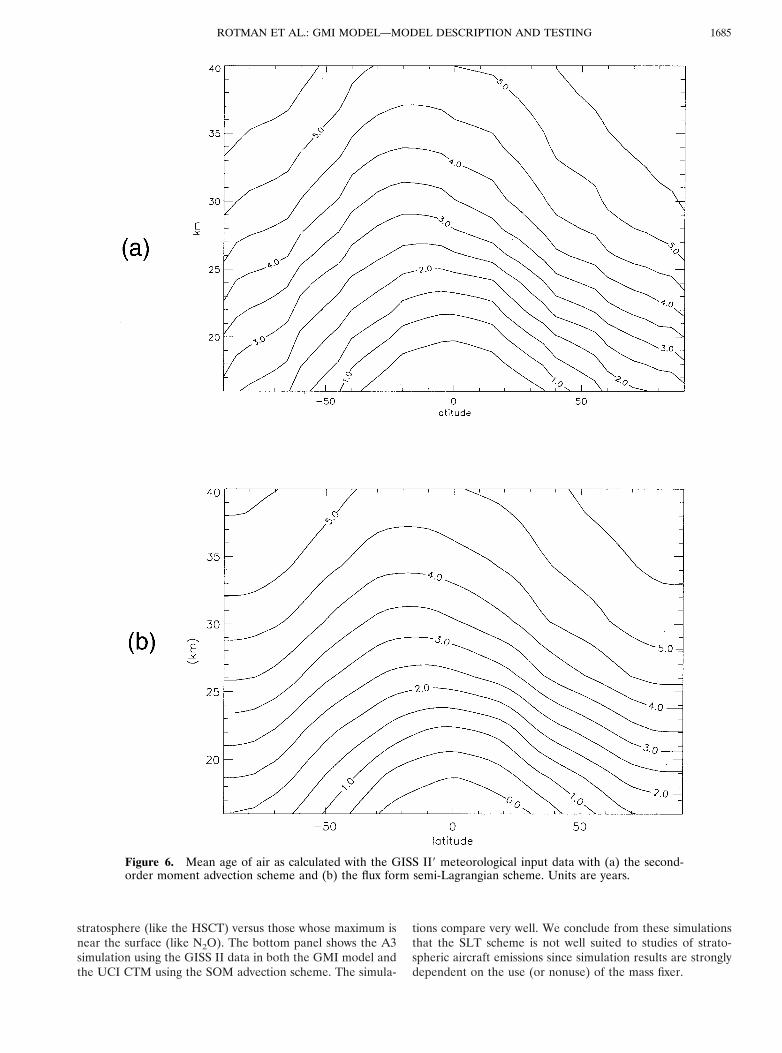
stratosphere (like the HSCT) versus those whose maximum isnear the surface (like N2O). The bottom panel shows the A3simulation using the GISS II data in both the GMI model andthe UCI CTM using the SOM advection scheme. The simula-

tions compare very well. We conclude from these simulationsthat the SLT scheme is not well suited to studies of strato-spheric aircraft emissions since simulation results are stronglydependent on the use (or nonuse) of the mass fixer.

Figure 6. Mean age of air as calculated with the GISS II9 meteorological input data with (a) the second-order moment advection scheme and (b) the flux form semi-Lagrangian scheme. Units are years.


Distributions in the first column of Figure 7 show only theinfluence of input meteorological data on the HSCT emissiondistribution (all other aspects of the model were held con-stant). Studies carried out in MMII showed the mean age inthe DAO meteorological data to be less than those of theMACCM2 and GISS II9 [see Park et al., 1999]. Distributions inFigure 7 suggest that for those models with lower mean ages(DAO), they accumulate less exhaust material in the lowerstratosphere. Recent work by Hall and Waugh [2000] suggeststhere may be a more quantitative relationship, albeit not per-fect, between mean age and buildup of aircraft emissions. Forexample, they suggest that a mean age of 3 years suggests atypical residence time of aircraft emissions of 1.1 to 2.1 years,while reducing the mean age to 2 years reduces the residencetime to 0.6 to 1.2 years. For more discussion of this subject, seeKawa et al. [1999].

8. Sensitivity of Simulations to AdvectionScheme Parameters

The GMI model’s primary advection algorithm is the fluxform semi-Lagrangian transport (FFSLT) [Lin and Rood,1996]. Within its algorithmic structure there are multiplechoices for monotonicity constraints that have implications onthe subgrid tracer distribution used to calculate fluxes acrosscell edges. In an effort to understand the sensitivities of tracersimulations to the selection of these constraints, we have car-ried out further simulations of MM II A1 and A3 using theFFSLT scheme. In the nomenclature of the FFSLT schemethese various choices are referred to as ORDs, and one haschoices of these constraints in the horizontal and vertical di-rections (i.e., IORD, JORD, and KORD). In our simulationsthe sensitivities seem to be small with respect to IORD and

Figure 7. Steady state simulations of NOx-like aircraft emissions (NASA MMII tracer A3). (top) Resultsfrom a 48 by 58 horizontal resolution simulation (GMI/DAO) and a 28 by 2.58 horizontal resolution (GSFC-3-D) using the NASA DAO assimilation input data. Simulations show higher horizontal resolution to isolatetracer to emission region. (middle) Results from MACCM2 input data in the flux form semi-Lagrangiantransport algorithm and the semi-Lagrangian algorithm. Differences were attributable to the use of a massfixer in the semi-Lagrangian algorithm. (bottom) Good agreement between the flux form semi-Lagrangian andsecond-order moment advection schemes. Units are ppbv.


JORD; however, important differences appear when alteringthe KORD. We will show these differences using the MMII A1and A3 tracer using FFLST and the GISS II winds. Similardifferences occur when using the DAO and NCAR data sets,but the differences are smaller (we will use this fact to betterunderstand our results).

Figure 8 shows the MMII A1 tracer run SOM and FFSLTwith the GISS II data set. Figure 8a shows output using theUCI-SOM advection scheme. Figure 8b represents FFSLTsimulations using KORD 5 3, while those in Figure 8c repre-sents those from a run using KORD 5 5. The KORD 5 5results match the original UCI-produced age very well (andwas used in Figure 6). However, when using KORD 5 3, theage of the stratosphere is much younger; by nearly 2 years.Recall, these KORD values represent different choices ofmonotonicity constraints and, in general, one can associatereduced diffusion with increasing values of KORD (for detailson the exact definitions of the KORD parameters, see Lin and

Rood [1996, Appendix A.3]. Figure 9 shows simulations of theMM II A3 tracer which also show large differences in thebuildup of tracer emissions in the lower stratosphere whenusing KORD 5 3 (Figure 9a) and KORD 5 5 (Figure 9b).Further investigations showed these differences to be relatedto vertical resolution. While these comparison simulationswere done with all the meteorological data sets, the GISS II setproduced the most marked differences. The GISS II set alsohas the coarsest vertical resolution in the tropopause region,identical to the region of tracer input. This is likely one of thecauses that leads to the larger differences in the GISS II9.Differences when using KORD 5 5 or KORD 5 3 appear tobe problem-dependent. Figure 4 showed N2O distributionsusing FFSLT and GISS II9 winds. In this case, the solution wassmoother through the tropopause region, and the results didnot depend on the choice of KORD.

By design, the GMI model allows these types of comparisonsimulations to be carried out and greatly aids in the under-

Figure 8. NASA MMII A-1 age diagnostic using the GISS II9 input meteorological data. Figure shows thesecond-order method scheme results and those of two versions of the flux form semi-Lagrangian (FFSLT)method. Case A of the FFSLT used a monotonicity constraint that allowed no overshoots and undershoots.Case B of the FFSLT used a monotonicity constraint that allowed only overshoots (remained positivedefinite). Results show the simulations to be highly dependent on this constraint. Analysis showed thedependence to be attributable to the constraint and the coarse vertical resolution of the GISS II9 data in theregion of the tropopause. Units are years.


Figure 9. Steady state NOx-like tracer using the flux form semi-Lagrangian transport algorithm and theGISS II9 meteorological data. Simulation results show a large difference in buildup of aircraft emissionsdepending on the advection algorithm characteristics: (a) with monotonicity constraint allowing no overshootsand undershoots and (b) allowing only overshoots (remains positive definite). Analysis showed this depen-dence to be attributable to the constraint and the coarse vertical resolution of the GISS II9 data in the regionof the tropopause. Units are ppbv.


standing of model simulations. This analysis can also be ex-tended to other results. For example, the MMII report [Park etal., 1999] shows large variations in simulation results from theMM II A3 tracer (and others). Given the variations seen bysimply changing the monotonicity constraint in the advectionscheme in the GMI model, one could argue that differentadvection schemes, different meteorological data, and differ-ent model structures throughout the entire MM II model suiteshould easily be able to produce the variety of results seen inthe simulation output. Such variations also point to the needfor GMI-type frameworks where science modules can be in-terchanged and intercompared. Moreover, this capability cou-pled with comparisons to observations (such as Douglass et al.[1999] and J. M. Rodriguez et al. (manuscript in preparation,2000)) provide an important pathway toward improved under-standing of assessment simulations.

9. ConclusionsThe NASA High Speed Research Program was tasked with

providing an assessment of the possible environmental conse-quences caused by the emissions of a proposed fleet of super-sonic aircraft. Past aircraft assessments made use of two-dimensional chemical transport models to provide impacts ofthe emissions on stratospheric ozone. Measurements and sim-ulations have both pointed toward the need for three-dimensional models to accurately assess the response of lowerstratospheric ozone. The NASA Global Modeling Initiativeand its science team was created to provide a robust, welltested and evaluated, and computationally advanced three-dimensional chemical transport model to provide assessmentsimulations and analysis. This model and framework is re-ferred to as the GMI core model. We have described a mod-eling structure designed to allow controlled numerical experi-mentation to better understand model simulations towardenabling a more robust and well understood assessment sim-ulation. The model structure allows intercomparison and diag-nosis of individual physics and numerical modules and allowsan understanding of sensitivities of simulation results to thenumerical algorithms and chemical/physical approaches taken.Extensive comparisons to observations are given by Douglass etal. [1999] and J. M. Rodriguez et al. (manuscript in prepara-tion, 2000). The model runs on a variety of platforms includingmassively parallel computers. We have used this model toproduce assessment simulations of a proposed fleet of super-sonic aircraft [Kawa et al., 1999; Kinnison et al., this issue].

The framework includes three different meteorological in-puts (NASA DAO, NCAR MACC2, and the GISS II9), threedifferent advection schemes (flux form semi-Lagrangian, semi-Lagrangian, and the second-order moment method), two dif-ferent numerical algorithms for chemistry solutions(SMVGEAR II and the semi-implicit method), along withalgorithms to provide mass consistent meteorological data,heterogeneous chemical processes on type 1 and type 2 polarstratospheric clouds, and diagnostics for model simulationanalysis. Simplified parameterizations for tropospheric physicsare included to wet deposit chemical species. The chemicalmechanism is focused on stratospheric chemistry with simpli-fied chemistry in the troposphere (i.e., methane). The mecha-nism includes photolytic and thermal reactions of species in thespecies families of Ox, NOy, ClOy, HOy, BrOy, CH4, and itsoxidation products. Photolysis rates are provided by a lookuptable.

To evaluate the model performance in the transport ofchemical species, we have applied the GMI core model to theNASA Model and Measurement II tracer tests: MMII A1 (agediagnostic) and MMII A3 (aircraft-emitted NOx-like tracer) aswell as N2O. The model was tested to ensure accurate imple-mentation of the numerical algorithms and was also applied tounderstand the sensitivity of meteorological input data andnumerical algorithms to simulated tracer transport. Studiesdiscussed in this paper show the models to faithfully reproducesimulation results from the data/algorithm parent organiza-tion. The ability of the model to swap numerical algorithmsand input data enabled the model to examine the sensitivity ofalgorithms and input data on simulation results. Results showthe N2O tracer to be relatively independent of numerical al-gorithm; however, the tracers of the age diagnostic and theaircraft NOx-like tracer are shown to be very dependent on thenumerical algorithm used in the advection operator.

Future work with the GMI model will extend its applicationto more meteorological data sets and more detailed tropo-spheric chemistry and transport, where, for example, the modelcan be used to study the influence of convective transportformulation on species distributions. A particular applicationwill be studying the perturbation caused by the emissions fromcurrent and projected fleets of subsonic (commercial) aircraftand analyzing the impacts on ozone and ozone chemistry withpossible feedbacks to clouds and climate.

Acknowledgments. The authors would like to thank the entireGMI Science Team for their collaborative effort toward this model.We would also like to thank Steve Baughcum for his many commentson this document. This work was performed under the auspices of theU.S. Department of Energy by the Lawrence Livermore NationalLaboratory under contract W-7405-ENG-48. Lawrence Livermore au-thors were supported by NASA contract S-10161-X.

ReferencesAlbritton, D. L., et al., The Atmospheric Effects of Stratospheric

Aircraft: Interim assessment report of the NASA High-Speed Re-search Program, NASA Ref. Publ., 1333, 1993.

Anderson, D. E., R. DeMajistre, S. Lloyd, and P. Swaminathan, Im-pact of aerosols and clouds on the troposphere and stratosphereradiation field with application to twilight photochemistry at 20 km,J. Geophys. Res., 100, 7135–7145, 1995.

Andrews, D. G., and M. E. McIntyre, Planetary waves in horizontaland vertical shear: The generalized Eliassen-Palm relation and thezonal mean acceleration, J. Atmos. Sci., 33, 2031–2048, 1976.

Baughcum, S. L., and S. C. Henderson, Aircraft emission scenariosprojects in year 2015 for the NASA Technology Concept Aircraft(TCA) High Speed Civil Transport, NASA Contract. Rep., CR-1998-207635, 1998.

Boville, B. A., J. R. Holton, and P. W. Mote, Simulations of thePinatubo aerosol cloud in general circulation model, Geophys. Res.Lett., 18, 2281–2284, 1991.

Brown, S. S., R. K. Talukdar, and A. R. Ravishankara, Rate constantsfor the reaction OH 1 NO2 1 M3 HNO3 1 M under atmosphericconditions, Chem. Phys. Lett., 299, 277–284, 1999.

Carslaw, K. S., B. Luo, and T. Peter, An analytic expression for thecomposition of aqueous HNO3-H2SO4 stratospheric aerosols includ-ing gas phase removal of HNO3, Geophys. Res. Lett., 22, 1877–1880,1995.

Chipperfield, M. P., D. Cariolle, P. Simon, R. Ramaroson, and D. J.Lary, A three-dimensional modeling study of trace species in thearctic lower stratosphere during winter 1989–1990, J. Geophys. Res.,98, 7199–7218, 1993.

Claveau, J., and R. Ramaroson, First simulation of the transport andthe chemical transformation of chemical species with a mesoscale-regional model: MEDIUM, paper presented at International Col-


loquium on Effects of Aircraft Upon the Atmosphere, Off. Natl.d’Etud. et Rech. Aerosp., Paris, France, Oct. 15–18, 1996.

Considine, D. B., A. R. Douglass, P. S. Connell, D. E. Kinnison, andD. A. Rotman, A polar stratospheric cloud parameterization for thethree-dimensional model of the global modeling initiative and itsresponse to stratospheric aircraft emissions, J. Geophys. Res., 105,3955–3975, 2000.

DeMore, W. B., S. P. Sander, D. M. Golden, R. F. Hampson, M. J.Kurylo, C. J. Howard, A. R. Ravishankara, C. E. Kolb, and M. J.Molina, Chemical kinetics and photochemical data for use in strato-spheric modeling, Evaluation 12, JPL Publ., 97-4, 1997.

Douglass, A. R., M. A. Carroll, W. B. DeMore, J. R. Holton, I. S. A.Isaksen, and H. S. Johnston, The Atmospheric Effects of Strato-spheric Aircraft: A current consensus, NASA Ref. Publ., 1251, 1991.

Douglass, A. R., R. B. Rood, C. J. Weaver, M. C. Cerniglia, and K. F.Brueske, Implications of three-dimensional tracer studies for two-dimensional assessments of the impact of supersonic aircraft onstratospheric ozone, J. Geophys. Res., 98, 8749–8963, 1993.

Douglass, A. R., R. Rood, S. Kawa, and D. Allen, A three-dimensionalsimulation of the evolution of the middle-latitude winter ozone inthe middle stratosphere, J. Geophys. Res., 102, 19,217–19,232, 1997.

Douglass, A. R., M. P. Prather, T. M. Hall, S. E. Strahan, P. J. Rasch,L. C. Sparling, L. Coy, and J. M. Rodriguez, Choosing meteorolog-ical input for the global modeling initiative assessment of high-speedaircraft, J. Geophys. Res., 104, 27,545–27,564, 1999.

Dunkerton, T., On the mean meridional mass motions of the strato-sphere and mesosphere, J. Atmos. Sci., 35, 2325–2333, 1978.

Gear, W., The numerical integration of ordinary differential equations,Math. Comput., 21, 146–156, 1967.

Gierczak, T., J. B. Burkholder, and A. R. Ravishankara, Temperaturedependent rate coefficient for the reaction O(3P) 1 NO23 NO 1O2, J. Phys. Chem. A, 103, 877–883, 1999.

Goldfarb, L., M. H. Harwood, J. B. Burkholder, and A. R. Ravishan-kara, Reaction of O(3P) with ClONO2: Rate coefficients and yieldof NO3 product, J. Phys. Chem. A, 102, 8556–8563, 1998.

Graedel, T. E., Statement before the Subcommittee on Technology,Environment, and Aviation, Committee on Science, Space, andTechnology, U.S. House of Representatives, Washington, D. C.,1994.

Hall, T. M., and D. Waugh, Stratospheric residence time and its rela-tionship to mean age, J. Geophys. Res., 105, 6773–6782, 2000.

Hall, T. M., D. Waugh, K. Boering, and A. Plumb, Evaluation oftransport in stratospheric models, J. Geophys. Res., 104, 18,815–18,839, 1999.

Hanson, D., and K. Mauersberger, Laboratory studies of the nitric acidtrihydrate: Implications for the south polar stratosphere, Geophys.Res. Lett., 15, 855–858, 1988.

Hartley, D. E., D. Williamson, P. Rasch, and R. Prinn, Examination oftracer transport in the NCAR CCM2 by comparison of CFCl3 sim-ulations with ALE/GAGE observations, J. Geophys. Res., 99, 12,855–12,896, 1994.

Hofmann, D. J., and S. Solomon, Ozone destruction through hetero-geneous chemistry following the eruption of El Chichon, J. Geophys.Res., 94, 5029–5041, 1989.

Intergovernmental Panel on Climate Change (IPCC), Special Reporton Aviation and the Global Atmosphere, edited by J. E. Penner et al.,Cambridge Univ. Press, New York, 1999.

Jacobson, M. Z., Computation of global photochemistry withSMVGEAR II, Atmos. Environ., Part A, 29, 2541–2546, 1995.

Kasten, F., Falling speed of aerosol particles, J. Appl. Meteorol., 7,944–947, 1968.

Kawa, S. R., et al., Assessment of the effects of high-speed aircraft inthe stratosphere: 1998, NASA Tech. Pap., TP-1999-209237, 1999.

Kinnison, D. E., et al., Global Modeling Initiative assessment model:Application to high-speed civil transport perturbation, J. Geophys.Res., this issue.

Lambert, J. D., Computational Methods in Ordinary Differential Equa-tions, John Wiley, New York, 1974.

Lin, S.-J., and R. B. Rood, Multi-dimensional Flux-Form Semi-Lagrangian transport schemes, Mon. Weather Rev., 124(9), 2046–2070, 1996.

Lipson, J. B., M. J. Elrod, T. W. Beiderhase, L. T. Molina, and M. J.Molina, Temperature dependence of the rate constant and branch-ing ratio for the OH 1 ClO reaction, J. Chem. Soc. Faraday Trans.,93, 2665–2673, 1997.

Logan, J. A., Nitrogen oxides in the troposphere: Global and regionalbudgets, J. Geophys. Res., 88, 10,785–10,807, 1983.

Marti, J., and K. Mauersberger, A survey and new measurements of icevapor pressure at temperatures between 170 and 250 K, Geophys.Res. Lett., 20, 363–366, 1993.

Mirin, A. A., et al., Climate system modeling using a domain and taskdecomposition message-passing approach, Comput. Phys. Commun.,84, 278–296, 1994.

Oort, A. H., Global atmospheric circulation statistics, 1958–1983,NOAA Prof. Pap., 14, 1983.

Park, J., M. K. W. Ko, R. A. Plumb, and C. Jackman (Eds.), Report ofthe 1998 Models and Measurements Workshop II, NASA Tech.Memo., TM-1999-209554, 1999.

Peter, T., C. Bruhl, and P. Crutzen, Increase in the PSC-formationprobability caused by high-flying aircraft, Geophys. Res. Lett., 18,1465–1468, 1991.

Prather, M. J., Numerical advection by conservation of second-ordermoments, J. Geophys. Res., 91, 6671–6681, 1986.

Prather, M. J., and E. E. Remsberg (Eds.), The Atmospheric Effects ofStratospheric Aircraft: Report of the 1992 Models and Measure-ments Workshop, NASA Ref. Publ., 1292, 1993.

Prather, M., M. McElroy, S. Wofsy, G. Russell, and D. Rind, Chem-istry of the global troposphere: Fluorocarbons as tracers of air mo-tion, J. Geophys. Res., 92, 6579–6613, 1987.

Prather, M. J., H. L. Wesoky, R. C. Miake-Lye, A. R. Douglass, R. P.Turco, D. J. Wuebbles, M. K. W. Ko, and A. L. Schmeltekopf, TheAtmospheric Effects of Stratospheric Aircraft: A first program re-port, NASA Ref. Publ., 1272, 1992.

Ramaroson, R., Local, one and three dimensional modeling of chem-ical processes in the middle atmosphere, Ph.D. thesis, Univ. ParisVI, Paris, France, 1989.

Ramaroson, R., D. Cariolle, and M. Pirre, Simulation of Noxon Cliffin a three-dimensional model with diurnal variations during an un-perturbed winter, in Proceedings of the First European Workshop onPolar Stratospheric Ozone Research, Schlieersee FRG, 3–5 October1990, edited by J. Pyle, N. R. P. Harris, Cambridge, England, 1991.

Ramaroson, R., M. Pirre, and D. Cariolle, A box model for on-linecomputations of diurnal variations in multidimensional models: Ap-plication to the one-dimensional case, Ann. Geophys., 10, 416–428,1992a.

Ramaroson, R., M. Pirre, and D. Cariolle, Qualitative study of thebehavior of minor species during a stratospheric warming with a 3-Dmodel, paper presented at Quadrennial Ozone Symposium, Int.Ozone Comm., Charlottesville, Va., June 1992b.

Rasch, P. J., and D. L. Williamson, Sensitivity of a general circulationclimate model to the moisture transport formulation, J. Geophys.Res., 96, 13,123–13,137, 1991.

Rasch, P. J., X. Tie, B. A. Boville, and D. L. Williamson, A three-dimensional transport model for the middle atmosphere, J. Geophys.Res., 99, 999–1017, 1994.

Rasch, P. J., B. A. Boville, and G. P. Brasseur, A three-dimensionalgeneral circulation model with coupled chemistry for the middleatmosphere, J. Geophys. Res., 100, 9041–9071, 1995.

Russell, G., and J. Lerner, A new finite differencing scheme for thetracer transport equation, J. Appl. Meteorol., 20, 1483–1498, 1981.

Sausen, R., et al., The impact of NOx emissions from aircraft upon theatmosphere at flight altitudes 8–15 km, in AERONOX, edited by U.Schumann, Comm. of the Eur. Communities contract EV5V-CT91-0044, Deutsche Luft-und Raumfahrt, Wessling, Germany, 1995.

Shimazaki, T., and A. R. Laird, A model calculation of the diurnalvariations of minor constituents in the mesosphere and lower ther-mosphere including transport effects, J. Geophys. Res., 75, 3221–3235, 1970.

Solomon, S., R. R. Garcia, F. S. Roland, and D. J. Wuebbles, On thedepletion of Antarctic ozone, Nature, 321, 755–758, 1986.

Stolarski, R. S., et al., 1995 scientific assessment of the atmosphericeffect of stratospheric aircraft, NASA Ref. Publ., 1381, 1995.

Tabazadeh, A., O. B. Toon, and E. Jensen, Formation and implicationsof ice particle nucleation in the stratosphere, Geophys. Res. Lett., 24,2007–2010, 1997.

Thomason, L. W., L. R. Poole, and T. Deshler, A global climatology ofstratospheric aerosol surface area density deduced from Strato-spheric Aerosol and Gas Experiment II measurements: 1984–1994,J. Geophys. Res., 102, 8967–8976, 1997.

Thompson, A. M., R. R. Friedl, and H. L. Wesoky, Atmospheric


effects of aviation: First report of the Subsonic Assessment Project,NASA Ref. Publ., 1386, 1996.

Weaver, C. J., A. R. Douglass, and R. B. Rood, Tracer transport forrealistic aircraft emission scenarios calculated using a three-dimensional model, J. Geophys. Res., 100, 5203–5214, 1995.

Weaver, C. J., A. R. Douglass, and D. B. Considine, A 5-year simula-tion of supersonic aircraft emission transport using a three-dimensional model, J. Geophys. Res., 101, 20,975–20,984, 1996.

World Meteorological Organization (WMO), Scientific assessment ofozone depletion: 1994, Rep. 37, Global Ozone Res. and Monit. Proj.,Geneva, 1994.

World Meteorological Organization (WMO), Scientific assessment ofozone depletion: 1998, Rep. 44, Global Res. and Monit. Proj., Ge-neva, 1999.

D. Bergmann, P. S. Connell, D. Proctor, D. A. Rotman, and J. R.Tannahill, Lawrence Livermore National Laboratory, Mail Stop Li-103, Livermore, CA 94550. ([email protected])

D. B. Considine, Department of Meteorology, University of Mary-land, College Park, MD 20742.

S. R. Kawa, S. J. Lin, and R. B. Rood, NASA Goddard Space FlightCenter, Greenbelt, MD 20771-0001.

D. E. Kinnison and P. J. Rasch, National Center for AtmosphericResearch, Boulder, CO 80307.

M. J. Prather, Department of Earth System Science, University ofCalifornia at Irvine, Irvine, CA 92697-3100.

R. Ramaroson, Office National d’Etudes et Recherches Aerospa-tiales, 92322 Chatillon, France.

J. M. Rodriguez, Department of Marine and Atmospheric Chemis-try, University of Miami, Miami, FL 33149-1098.

(Received May 3, 2000; revised July 31, 2000;accepted August 2, 2000.)


Global Modeling Initiative assessment model: Model ...

Documents

Transcript of Global Modeling Initiative assessment model: Model ...