J . Fluid Mech. (1993), vol. 251, pp. 1-20 Copyright Q 1993 Cambridge Univer5it.y Press

1

Global linear stability analysis of weakly non-parallel shear flows

By PETER A. MONKEWITZ’, PATRICK HUERRE2 AND JE AN-M ARC CHOMAZ2

Department of Mechanical, Aerospace & Nuclear Engineering, University of California, Los Angeles, CA 90024-1597, USA

* Laboratoire d’Hydrodynamique (LADHYX), Ecole Polytechnique, 91 128 Palaiseau Gdex, France

(Received 22 April 1992 and in revised form 7 August 1992)

The global linear stability of incompressible, two-dimensional shear flows is investigated under the assumptions that far-field pressure feedback between distant points in the flow field is negligible and that the basic flow is only weakly non- parallel, i.e. that its streamwise development is slow on the scale of a typical instability wavelength. This implies the general study of the temporal evolution of global modes, which are time-harmonic solutions of the linear disturbance equations, subject to homogeneous boundary conditions in all space directions. Flow domains of both doubly infinite and semi-infinite streamwise extent are considered and complete solutions are obtained within the framework of asymptotically matched WKBJ approximations. In both cases the global eigenfrequency is given, to leading order in the WKBJ parameter, by the absolute frequency wo(Xt) at the dominant turning point 2 of the WKBJ approximation, while its quantization is provided by the connection of solutions across Xt. Within the context of the present analysis, global modes can therefore only become time-amplified or self-excited if the basic flow contains a region of absolute instability.

1. Introduction The present paper addresses the extension of the concept of absolute instability to

non-parallel flows. As in the case of parallel flows, in which an initial impulsive excitation leads to the ultimate dominance of the most amplified Fourier or normal mode with zero group velocity (Briggs 1964; Bers 1983, etc.), we attempt to answer the question of the asymptotic (in time) impulse response of a non-parallel flow and we will call the equivalent of the ‘absolute’ normal mode a linear ‘global’ mode. The latter is simply a time-harmonic solution of the homogeneous linearized disturbance equations with homogeneous boundary conditions in space. Such solutions can in general be obtained only numerically, especially if the basic flow is strongly non- parallel. Examples of such computations in shear flows have been published by Zebib (1987), Hannemann & Oertel (1989) and a few others.

If the mean flow is weakly non-parallel, i.e. varies slowly on the scale of a typical instability wavelength, global modes become accessible to WKBJ-type analyses. This involves the step from the ‘slowly diverging’ approach of Bouthier (1972) and Crighton & Gaster (1976), who treat the spatial evolution of a forced wave in an inhomogeneous medium (the signalling problem), to the problem of finding the unforced global modes where the streamwise direction also becomes an ‘eigenvalue

2 P . A . Monkewitz, P . Huerre and J . -M. C b z

direction ’. In the special situation where the flow and the destabilizing mode are invariant under the reflection x+ -x of the streamwisc coordinate, which results in absolute instability being synonymous with instability (Chomaz, Huerre & Redekopp 1991), global modes have been obtained in several cases. They include most notably the Taylor vortex problem in the gap between two concentric spheres, which has been treated comprehensively by Soward & Jones (1983). This paper also contains a brief discussion of spiral modes which break the x+ -x symmetry but the link to the absolute and convective nature of the instability is not established (for corresponding experiments see Buehler 1991). The basic ideas of this connection were laid out by Pierrehumbert (1984) in the context of the baroclinic instability of zonally varying flows. The same methods were used in other studies to investigate instabilities of Poiseuille flow in a curved pipe (Papageorgiou 1987) and instabilities of Saffman- Taylor fingers (Bensimon, Pel& & Shraiman 1987). Similar ideas have been pre- sented by Fuchs, KO & Bers (1981) and Landahl (1984). The common thread through all these analyses is the need, dictated by the boundary conditions, for different branches of the WKBJ-approximation in different flow regions, which have to be connected through a turning point region where the WKBJ-approximation breaks down.

In this paper we extend the ideas of Soward & Jones to the case of infinite or semi- infinite shear flows that contain regions of both absolute and convective instability. In other words, we pick up the discussion of Pierrehumbert (1984) and the model analyses of Chomaz, Huerre & Redekopp (1988) and Huerre & Monkewitz (1990) and present a complete analysis of two-dimensional global modes on shear flows in both semi-infinite and doubly infinite domains (see also Monkewitz, Huerre & Chomaz 1989), similar to the recent study of global modes in a thin galactic disc by Soward (1992). In particular, we take into account the cross-stream structure of the global modes and include an explicit discussion of the connection between the properties of global modes and local absolute and convective instability. This connection, which is supported by several examples (Monkewitz 1990), is put on firmer ground. We note, however, that the analysis admits only ‘local feedback’ by vorticity waves to drive global modes. It is therefore restricted to cases where long-range pressure feedback is negligible and important problems such as edge tones are not addressed, for which the primary driver of the instability is the acoustic feedback from a downstream point of intense fluid-surface interaction to a trailing edge.

The paper is organized as follows. In $2 the governing equations for incompressible, two-dimensional viscous flow are brought into a form suitable for the analysis. The study of the WKBJ-approximation to the Green function in non-parallel flows in $3 then provides a unified approach to the problem of frequency selection in both the doubly infinite and semi-infinite domains. The details of the analysis for both flow domains, including the matching between ‘inner’ solutions in the regions of WKBJ- breakdown and ‘ WKBJ-tails ’, are given in §$4 and 5, respectively. The concluding 0 6 discusses applications and possible extensions of the analysis, and the Appendices define the operator notation used throughout the text.

2. The basic equations To study two-dimensional instability waves in a spatially inhomogeneous,

incompressible medium, we start from the equation for the z-vorticity -V2Y, where !P is the total stream function and R is the Reynolds number:

Global linear stability of weakly non-parallel shear j lows

[a,+(a, Y)a,-(a, Y)ay]v2Y = R-'V2V2Y.

3

(2 .1)

Next, Y is decomposed into a time-independent mean flow $ and a small disturbance qY:

Y = $(X, y ) + V ; x = E X . (2.2)

At this point we assume that, in the terminology of the method of multiple scales (see e.g. Bender & Orszag 1978), the mean flow + depends only on the 'slow ' coordinate X = €5. The parameter

(2.3)

characterizes the degree of spatial inhomogeneity of the basic flow by providing a measure of the small change of the typical cross-stream lengthscale S(s) over one typical instability wavelength A,,,. In the absence of body forces, the assumption of a slow evolution of the mean flow immediately restricts viscous effects to O(s) , or in terms of the Reynolds number R

E = h,,,{6'(s)[dS/d~]},,, -4 I

R = C'R; R = O(1). (2-4)

Introduction of the decomposition (2.2) and of (2.4) into the governing equation (2.1) first leads to the boundary-layer equation for the basic flow

(a, $1 (3, a; $1 - (3, $) (a; $1 = R-' (3; $ 1 1 (2 .5a)

u(x,y) = a,$; v(x,y) = -a,$ = -€--'a,+. (2.5b)

Linearizing around the basic flow and keeping only terms up to O(E) then yields the following equation for the small disturbance $' :

[(a, + UaZ) v2 - (a; u) a,] II-' +e[Va,V2+ (a, a, U ) d,-R-' V2V2] $'+O(s2 I$'!, lfl2) = S(s , 9, t ) , (2.6)

where a, and the Laplacian V 2 have not yet been split into fast and slow parts. The source S has been added for the study of the impulse response in the next section, but the ultimate aim of the paper is the search for global modes, i.e. homogeneous solutions of (2.6) with homogeneous boundary conditions in space.

3. The WKBJ approximation for the evolution of instability waves and its breakdown

Following Bouthier (1972), Crighton &, Gaster (1976) and others, we use the WKBJ approximation up to the level of 'physical optics' (see e.g. Bender & Orszag 1978) to describe the evolution of instability waves on the weakly non-parallel basic flow. In a first part we discuss the WKBJ approximation to the Green function of (2.6) and identify the locations of its breakdown which are 'turning points' of the problem (see $10 of Bender & Orszag 1978). We conclude this section by fixing the notation and by bringing the results into a form suitable for the analyses of $$4 and 5 .

To obtain the Green function G of (2 .6) , the source at x = 9 and y = ys is specified as

(3.1) S(X, y, t ) = (S(z - x") + i[z(z - P)]--'} S(y - y") S(t) .

This form explicitly accounts for the non-analyticity of G on the imaginary axis of the wavenumber plane when the lateral extent of the flow domain is infinite, as

4 P . A . Monkewitz, P . Huerre and J.-M. Chomaz

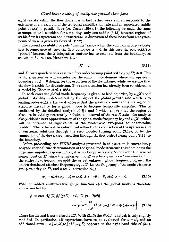
FIGURE 1. (a) Sketch of the Fourier inversion contour L in the complex w-plane with maps Mu and N, ofM and N , subject to a,w = 0. (b) The WKBJ integration path M in the complex X-plane for the doubly infinite flow domain with double-valued map X * of L, subject to a,w =O. (e) Corresponding path N and X' for the semi-infinite case. The top row (subscripts 1) shows the situation where L is above all singularities (O), while the bottom row (subscripts 2) shows the points (0) of the X-contour where the breakdown of the WKBJ-approximation can no longer be avoided as L is lowered.

discussed in detail by Huerre & Monkewitz (1985). Next, we take the Fourier transform of (2.6) in time according to

n

G(z, y, t ) = (2rc)-' 6(s, y, w ) exp ( - iwt) dw, (3.2) J, where the contour L is taken parallel to the real w-axis (figure la) and above all singularities in order to obtain a causal solution (Briggs 1964). Finally, all x- derivatives in the disturbance equation (2.6) are transformed according to the chain rule

a,+a,+ea,, (3.3)

keeping in mind that a, and a, do not commute. Concentrating on a flow domain of doubly infinite streamwise extent, G is required to vanish at up- and downstream infinity as well as on the lateral boundaries [y[ = 00. Hence, following Q 10.3 of Bender & Orszag ( 1 9 7 ~ the WKBJ approximation for 6 can be written in the standard form away from the source at x = 2:

&* - ( 6 ~ ( X , y ) + E b : ( X , y ) + O ( E l ) ) e x p [ i € - l ~ , ~ k ~ ( ~ ~ w ) ~ ] , X (3.4)

where 6 plays the role of the WKBJ-parameter. The superscripts ' + ' and ' - ' denote the approximation downstream and upstream of the source, respectively. The k * ( X ; w ) are the corresponding local wavenumbers in the upper and lower half k-plane, respectively, as shown on figure 2 ( b ) of Huerre & Monkewitz (1985). For simplicity we assume here that there is only a single pair of eigenvalues k*.

Global linear stability of weakly non-parallel shear flows 5

Introducing the WKBJ-Ansatz (3 .4 ) into the Fourier-transformed equation (2.6) the stability problem reduces, at leading order in E , to a streamwise succession of locally parallel problems which are governed by the homogeneous Rayleigh equation and associated boundary conditions in y. Thus, a t O(E') one obtains

O(E') : Y($f ; k* , w , X ) = 0 ; $f(ly(-+m) = 0 , ( 3 . 5 ~ )

with @f(X,y) = Af(X)$$(y;X). (3 .5b)

The solution depends only parametrically on X through the shape of the local mean velocity profile U(X,y) and yields k i as well as the local transverse structure of 8, up to an unknown amplitude A, (X) . The latter describes in essence the 'transmission ' of the instability wave from one locally parallel region to the next and will be determined at the next order. The Rayleigh operator 9, which includes a list of all relevant parameters in the argument, is defined as (see also Appendix A)

(3 .6 )

At linear order in E, the following inhomogeneous Rayleigh equation for @ is

dip( - ; k , W , X ) [kU(y ; X ) - W ] [a: - k2] - - k[aE U( y ; X ) ] - .

obtained :

O ( 8 ) : 9(8: ; k * , w , X ) = iY, ($: ; k* , w , X ) a, Af + i { 9 k ( a x $f ; k', 0 , X ) + t Y k k ( $ f ; k', w , x ) a, k + 9c($t ; k', w , X ) } A $ , (3 .7 )

where the derivatives of the operator Y are defined in Appendix A. It will prove useful to replace a, $8 by the expression (C 4 ) of Appendix C where the functions $h, etc. are defined by (C 5). In order to avoid secular terms in the solution of (3 .7 ) , a solvability condition has to be satisfied. After dividing by LJ$$ ; k * , w , X ) and using (B 4) for a ,w* , the condition reads

(3 .8 ) Gw*(w,X) = i [ L , ( $ f ; k ' , w , X ) - L , ( $ ~ , ; k * , o , X ) ] [ L , ( $ $ ; k * , w , X ) ] - ' , ( 3 . 9 ~ )

ak U* a, Af = - [i6w* +$&a, k' +d&a, w * ] Af ,

d & ( w , X ) [2L,($: , ;k*,o,X)-L, , ($$ ; k ' , w , X ) ] [ L , ( $ f ; k * , w , X ) J - ' , (3 .9b )

d&(U,X) Lk($:,;k*,U,X) [L,($f ; k * , w , X ) ] - ' . ( 3 .9c )

The L above are defined by (B 3 ) in Appendix B and represent inner products of the corresponding Y with the solution of the adjoint Rayleigh equation. As will be seen later, 6w is a frequency correction due to non-parallel and viscous effects. The coefficients d,, on the other hand, are related to the dispersion relation D associated with the local Rayleigh equation at X by d , = -a+D/a,D, e.g. d,, = -a:D/a,oD. Equation (3 .8) is now readily integrated to yield

A $ @ ) = A:* exp [ - 6 ~ * + ~ i d ~ , a , k * + i d ~ ~ a , w * ] ( X ; w ) ~ 3. (3 .10) a, W* (x ; w )

The notation in (3 .10) indicates that a, &(XI; w ) , etc. are to be evaluated for the local eigenvalue pairs ( k * , w ) at X . The approximate description of the Green function away from the source is thus brought from the level of 'geometrical optics', which is associated with the eikonal i s k ( X ) dX', to the level of 'physical optics'. The latter is required if one is to obtain an approximstion valid to O( 1) included. What remains to be done is the connection of 8; and 8: across the source. For this, the analysis in 8 10.3 of Bender & Orszag (1978) has to be generalized : instead of patching the two solutions 6; and @:, which is only possible for ODES, we use in essence the approach of Burridge & Weinberg (1977) in which the connection is achieved by matching 8;

6 P. A. Monkewitz, P. Huerre and J.-M. Chomaz

and 8: to the local parallgl Green function at X". The latter is obtained from the double Fourier transform G in time t and space x at X 7 Xs which is given as equation (8) in Huerre & Monkewitz (1985). Integration of G with respect t o k along the contours shown on figure 2 (b) of Huerre & Monkewitz (198.5) yields, upon evaluating the residues at k+ and k- respectively for frequencies on the contour I, of (3.2),

In this expression H is the Heaviside function ad D the dispersion relation associated with the local Rayleigh equation at X". We note that in (3.11) the contribution from the integration along the imaginary k-axis, which is a branch cut of the dispersion relation, has been omitted under the assumption that the long-time behaviour is dominated by the discrete spectrum. Comparison of (3.4), (3.5) and (3.10) with (3.11) finally yields

(3.12)

We now turn to the discussion of the long-time behaviour of G which runs analogous to the discussion of absolute and convective instability in the parallel case. The basic idea is that the leading-order time-asymptotic behaviour of G is determined by the uppermost singularity of 8 in the w-plane, i.e. the singularity with the largest temporal growth rate, which becomes 'pinned' as the w-contour is lowered. In the parallel case, the singularities in the o-plane, which correspond to zeros w(k) of the dispersion relation D, can be moved by deforming the Fourier-inversion contour in the k-plane until the latter is pinched between two branches k+(o) and k-(w) (see Briggs 1964; Bers 1983, etc.). When this occurs, the singularity wo E w(ko) becomes 'pinned ' at the absolute frequency wo which corresponds to the saddle point ko where the complex group velocity a,w is zero and the k-contour is pinched.

In the weakly non-parallel case we can argue in a completely analogous manner: if 8(X,w) becomes singular at a location X t from which the X-integration contour cannot be moved, the corresponding pole w(X) becomes 'pinned '. Again, the 'pinned ' pole with the largest temporal growth rate determines the time-asymptotic behaviour of G. From (3.10) it is seen that d , in particular Ao(X), becomes singular at the zeros of a k w . Such points are in fact turning points X t where the WKBJ- approximation breaks down, which is easily seen by noting the correspondence between Ao(X) and [&(X)]-' in standard textbook notation (see $10 of Bender & Orszag 1978). In the following, we have to distinguish between two types of pole 'pinning '.

The first is the exact analogue of the parallel case where the X-integration contour is pinched between two branches X*(w I akw = 0) on which the group velocity is zero. The pinching occurs at the saddle point, or second-order turning point X where

(3.13)

as shown on figure 1 (b). This is the case discussed in detail by Chomaz et al. (1991), which arises when the absolute growth rate wo,(X) has a maximum within the flow domain, and represents a generalization of Pierrehumbert's ( 1984) frequency selection criterion to the complex X-plane. The assumption that a maximum of

Global linear stability of weakly non-parallel shear f i w s 7

w,,(X) exists within the flow domain is in fact rather weak and corresponds to the existence of a maximum of the temporal amplification rate and an associated saddle point of w ( k ) in parallel flows (see Gaster 1968). In the following we make the same assumption and consider, for simplicity, only one saddle (3.13) between regions of stable flow far upstream and downstream. A discussion of these ideas from a physical point of view is given by Soward (1992).

The second possibility of pole 'pinning' arises when the complex group velocity first becomes zero at, say, the flow boundary X = 0. In this case the pole wo(Xt) is 'pinned ' because the X-integration contour has to emanate from the boundary, as shown on figure 1(c). Hence we have

P=O (3.14)

and X corresponds in this case to a first-order turning point with a, w 0 ( P ) 4= 0. This is the situation we will consider for the semi-infinite domain where the upstream boundary at X = 0 dominates the evolution of the disturbance while we assume that the flow is stable far downstream. The same situation has already been considered in a model by Chomaz et al. (1988).

In both cases the global mode frequency is given, to leading order, by w , ( X ) and global instability is determined by the sign of the global growth rate which is to leading order woi(X) . Hence it appears that the mean flow must contain a region of absolute instability for a global mode to become temporally amplified. This is confirmed by the detailed analysis of $94 and 5 which shows that the region of absolute instability necessarily includes an interval of the real X-axis. The analysis also yields the next approximation of the global mode frequency beyond wo(Xt) which will be obtained as eigenvalues of the streamwise two-point boundary-value problem. The latter will be determined either by the connection of the upstream and downstream solutions through the second-order turning point (3.13), or by the connection of the downstream solution through the first-order turning point (3.14) to the boundary.

Before proceeding, the WKBJ analysis presented in this section is conveniently adapted to the future determination of the global mode structure that dominates the long-time impulse response. First, it is no longer necessary to consider the general source location X", since the region around Xt can be viewed as a 'wave-maker' for the entire flow. Second, we split the as yet unknown global frequency wG into the known dominant absolute frequency w: at X , i.e. the frequency of the mode with zero group velocity a t X , and a small correction EO,:

wG = w : + w , ; w: = w ( k t , X ) with a,w(ki,X+) = 0. (3.15)

With an added multiplicative gauge function p(e) the global mode is therefore approximated by

Y = p(g){A~(x)q5$(Y;x)+s~:(x, Y ) + W ) l r rx 1

x exp 1ie-l J ,' k ' (X ; wk) dX' - i(w: + ewe) t , (3.16) 1 where the eikonal is normalized at Xt. With (3.15) the WKBJ analysis is only slightly modified. In particular, all expressions have to be evaluated for w = w: and an additional term -Af wt9Jq5$ ; k*, wk, X) appears on the right-hand side of (3.7),

8 P. A, Monkewitz, P. Huerre and J.-M. C b z

with a corresponding term iA$ w, on the right-hand side of (3.8). Equation (3.10) is thus modified to

We note that the integrand in (3.17) may have a simple pole at X in which case the integral is strictly speaking divergent. The integral is then to be interpreted in the following manner : rx rx

This concludes the analysis of the WKBJ 'tails ' of the global modes away from the turning points X. To complete the solution, the turning point regions have to be ' magnified ' and analysed.

4. The turning point region for the doubly-infinite flow domain In this section the ideas of Soward & Jones (1983)' Huerre & Monkewitz (1990) and

Chomaz et al. (1991) on global modes in a doubly infinite flow domain are applied to shear flows. In terms of applications, the following analysis may be useful not only in truly infinite domains, typically found in geophysical shear flows, but also in finite flow domains, as long as the boundaries do not significantly influence the flow instability. The two-dimensional bluff-body wake appears to be a case in point as suggested by Monkewitz (1988) and the numerical experiment of Triantafyllou & Karniadakis (1990) who obtained essentially the same KarmBn vortex street after replacing the cylinder by an inflow boundary condition downstream of the cylinder.

4.1. Analysis of the turning point region

At the turning point defined by (3.13) the first-order equation (3.8) for A: becomes singular and one has to bring in the second derivative e23;A,$. Since X is also a saddle point of the absolute growth rate wo(X) , (w,-w:) behaves like (X-Xt)z. Hence X is a second-order turning point where the second derivative of Aof must be of the same order as (X-Xt)2A$ (see Bender & Orszag 1978). This leads immediately to the rescaling

In the inner turning point region, characterized by 1x1 < 0(1), the disturbance stream function is expanded accordingly :

where k: = k,(X). By the same token the global frequency w, is expanded around

R = Ed(X - F). (4.1)

= [Q, + dQ, + eQZ + 0(4] (1, y) exp [is-'k:(X -XI - iw, t ] , (4.2)

(4.3) wo(X') = 0::

wc = w: + B h , + B i j 2 + O(&

U ( X , y) - u(xt, y) +dx[a, v] (x, y) + E$P [a; (xt, y) + O(E;),

and the mean flow components are expanded in Taylor series around X'. In terms of the inner variable (4.1) they are given by

(4.44 V ( X , y) - V(Xt, y) + O(B$ (4.4b)

Introducing the expansions (4.2) and (4.4) aa well as the 'slow ' variable (4.1) (using the chain rule a, + a, +.&ax) into the governing equation (2.6) yields, at leading order in B , the local Rayleigh equation at Xt

O ( 8 ) : Y(&) = 0; $:(lyl-oo) = 0, (4.5)

10 P . A . Monkewitz, P . Huerre and J.-M. C h m z

(1990) and (5.24) of Soward (1992). The relation of (4.13) to the local dispersion relation becomes immediately transparent after transforming to the spectral domain with the substitution

a, += ie-f( k - k:) . (4.15)

Using (4.3) and (4.10) this yields the Taylor series representation of the frequency in the neighbourhood of the turning point X t

€G2 E 0 - w : = €so'+&d:k(k-kk)2+o:x(k-k: ) ( X - X t ) + & d i x ( X - X t ) 2 , ( 4 . 1 6 ~ )

with wbk = dtkk , wbx E d i x , w i , = d i X . (4.16 b)

The first term in (4.16a), ESW', arises from both non-parallel and viscous effects, while the last three terms represent the Taylor expansion of the inviscid dispersion relation w(k, X ) in the locally parallel approximation. Because of ak w(X') = a, w(X') = 0, its coefficients are directly related through (4.16b) to the corresponding expansion coefficients (4.14) of D(w, k , X ) . In order to keep this connection in view, we switch at this point to the more descriptive nomenclature wik , etc., wherever appropriate.

Taking the derivative of ( 4 . 1 6 ~ ) with respect to k , excluding the non-parallel correction Sw', the absolute wavenumber and frequency in the inner region are determined as

k,- k: = k k x ( X - X t ) ; kkx -w;X/wik, (4.17 a)

w 0 -w' 0 = b' 2 O X X ( X - X t ) 2 ; w:XX w ' , X - ( w k X ) 2 / w : k . (4.17b)

Hence we have shown that the relation (4.16), which had been discussed by Huerre & Monkewitz (1990) and postulated by Chomaz et al. (1991), is generic to the turning point region of the WKBJ approximation and can be derived in a rational fashion from the governing equations under rather weak assumptions. Furthermore, (4.17 b) proves that there is a location X, on the real X-axis, where Im[w,(X,)] 2 Im[w:] when Im [o:,,] < 0. This explicitly confirms the earlier statement that a region of absolute instability is necessary for global instability. The solution of (4.13) is now easily found by transforming it into the standard Hermite equation. For this, the new coordinate

6 = (4w~,,/w~k)~X (4.18)

is introduced with a choice of branch cut such that Re [c2] > 0. In addition, the first derivative in (4.13) is eliminated by setting

A, (X) = exp [$kk,X2]a([) . (4.19)

We note that the argument of the exponential is nothing other than the second term in the expansion of the eikonal i[ki(z - z') + E-'S (k , - k:) a], where the integral is taken from X' to X. With (4.18) and (4.19), (4.13) finally takes on the standard form

- -

a%ol+a([G2-8W'+$& k : , ] [ ~ ~ k ~ : x x ] - ~ - ~ 6 ~ } = 0, a(l6l-f 00) = 0. (4.20)

The boundary conditions ensure the matching to the subdominant WKBJ solutions both upstream and downstream of X and restrict the frequency correction G, to the following set of discrete eigenvalues :

e2, = dWt -$U:k k:x -k (n -k i) ((& W ~ X X ) ~ . (4.21 a)

The branch cut in (4.21a) is chosen so as to yield a negative imaginary part for in keeping with the general discussion of Soward (1992). The global

eigenfunctions corresponding to Gtn are given by

(4.21 b) a n ( 6 ) = ~ X P [-iE21Hen(E),

Global linear stability of weakly non-parallel shear flows 11

where the He,(f[) are Hermite polynomials as defined by Abramowitz & Stegun (1965). With (4.21b) the free overall amplitude of the linear global mode has been normalized such that a,(X = Xt) = 1. We reiterate here that, according to the discussion leading to the frequency selection criterion (3.13), the global mode (4.21) represents the asymptotic solution for long times. The recent feat of Hunt & Crighton (1991) who determined the exact Green function of (4.13) puts us into the unique position of verifying this statement explicitly. If the limit t + co is taken in their expression (36) and (44) for the Green function, one indeed recovers the most unstable global mode (4.21) with n = 0. The higher modes are more stable since the imaginary parts of w',, and w i X x are negative, corresponding to a high-wavenumber 'cutoff' and to stability at (XI + 00 respectively. A t this point the solution of (2.6) in the inner or turning point region is complete and the only task left is the matching of the WKBJ-'tails' to the inner solution.

4.2. Matching with the WKBJ approximations For large 1x1, i.e. far away from the turning point X , and for low-order modes [n = O(l ) ] the asymptotic expansion of the solution (4.19) and (4.21) may be used (Abramowitz & Stegun 1965) which yields the leading-order aaymptotics of the inner solution (4.2) for the nth global mode:

3,(1X1 +a, y) - (4wt,,,/w',,)n/4Xn@( 0 Y 1 e XP { - g2[(wt,xx/w',,)' - %XI}

x exp{ik:(x-xt)-i(w:+ea2,)t}. (4.22)

To match to the outer WKBJ-approximation (3.16) the latter has to be investigated for X approaching the turning point X. To approximate the integrals in (3.16) and (3.17) we use the Taylor expansion ( 4 . 1 6 ~ ) of the frequency to obtain the following leading-order approximations :

k k ( X ; w t , ) - k ; - [k:,+i(wt,,,/w',,)l](X-Xt)+ ..., (4.23)

where the branches of the square root have been selected so as to yield the subdominant solutions both down- and upstream of P. Hence we obtain

( 4 . 2 4 ~ )

a , w ' ( ~ ; w t , ) - i(w',,wk,,)$Y-X)+ ... . (4.243)

With (4.23), (4.24) and setting w, = a2,, given by (4.21 a), the expression (3.17) for A$ can be approximated for X + X , noting that &J(X+x", y) + &,(y), Sw*(X+X')+Sw' and d & ( X + X ) + d ' , , = w:, (compare ( 3 . 9 ~ ) and (3.9b) to ( 4 . 1 4 ~ ) and (4.14b) respectively). The outer solution (3.16) for the nth global mode thus behaves, to leading order, as

$;*(~+x", y) - p(e) ( x - X ) ~ A ~ &(y) exp { - ~ E - ~ ( x - x ~ ) ~ [ ( w ~ , ~ / w ~ ~ ) ~ - ikt,,]}

x exp{ik~(x-xt)-i(wt,+e~2,)t}. (4.25)

The asymptotic match of (4.25) and (4.22) is achieved if we set

p ( € ) = P ' 2 , At, = (4w;,,/w;,)n/4, (4.26a, b)

which concludes the leading-order analysis of global modes on a doubly infinite flow domain containing a single dominant saddle point of the absolute growth rate in its interior. To avoid misunderstandings it is worth pointing out here that the notion of

12 P. A . Monkewitz, P. Huerre and J . - M . Chomaz

WKBJ-'tails' does not in any way imply that the amplitude of the global mode should peak near the turning point which acts as the 'wave-maker' for the entire flow. Depending on the imaginary part of k', and the downstream evolution of I m [k+] the wave 'leaking' from the ' wave-maker ' region can experience substantial spatial amplification. In such cases the maximum amplitude is found, to leading order in the WKBJ parameter, where Im [k+] = 0 (see Crighton & Gaster 1976). In laboratory terms this means that the location with the most conspicuous oscillations generally does not coincide with the dynamically most active region which is around the real part of X t , if X' is close to the real axis. When looking for the forcing location that is most effective in modifying global oscillations, one finds still another region, shown by Chomaz, Huerre & Redekopp (1990) to be upstream of the active neighbourhood of x.

5. The turning point region for the semi-infinite flow domain In this section the model investigated by Chomaz et al. (1988) is re-examined in the

context of the present rational asymptotic analysis, starting from the governing equation (2.6). The main assumption, besides the exclusion of long-range feedback, is that the flow is most (absolutely) unstable at the boundary, i.e. that the location of the 'wave maker' is given by (3.14), and that a, wo(Xt) + 0, i.e. that w,(X) has no saddle point at X . Furthermore we will assume that the global mode amplitude is zero at the boundary X = 0.

5.1. Analysis of the turning point region The analysis is very similar to that of $4.1 and will be kept as brief as possible. Because of a, wo(Xt) =k 0, the absolute growth rate o,(X) is at leading order, a linear function of ( X - X t ) near X'. Therefore, the balance between 2 a; A: and ( X - P ) A? near X' leads to the scaling

It will prove advantageous not to use the leading-order result (3.4), i.e. X = 0, immediately, but to leave Xt unspecified at this point. Consistent with the scaling (5.1) the disturbance stream function is expanded as

$' = [6,+d6:, + E % ~ + E ~ ~ + O ( E ~ ) ] (%,y)exp[is-'k&X-X)-iw,t], (5.2)

x = €-:(X-Xt). (5.1)

where k', = ko(X t ) , and the global frequency is represented by

WG = (0: + €;GI + €:G2 + €G, + O(€$). (5.3)

Analogous to (4.4), the mean flow is expanded around X :

u(x, Y) - u ( x t , Y) +€%[a, vl (xt, Y) + o(4, (5.4a)

V ( X , y) - V ( P , y) + O ( 4 . (5.46)

This, together with the transformation of 2-derivatives according to a,4, + &a2 yields, at leading order, the Rayleigh problem at Xt

O ( E 0 ) : Yt($',) = 0 ; &( Iyl -KO) = 0, (5.5)

where the same notation has been used as in $4. The leading-order inner solution is thus determined up to a free amplitude Jo(x)

Global linear stability of weakly non-parallel shear flows 13

At the next order, one obtains the following first-order equation for 2, which differs from (4.8) because the mean flow is missing an O(&) term

o(&: yt(Z1) = iyi($i)a,Ao-Gl y:($k)Bo. (5.7)

The corresponding solvability condition reads

iLi($i) [L:(&,)I-~ a, X0 -&,a, = 0. (5.8)

The coefficient of a,x, in (5.8) is, according to (B 4), proportional to the complex group velocity at X', which vanishes because the global frequency is, to leading order, equal to the absolute frequency at P. Therefore

and the solution of (5.7) is 3, = 0, (5.9)

61(x? Y ) = $:(?/I + iaA?xO $ i k ( Y ) ? (5.10)

where q5:k is defined by (C 5 ) with k = kk, w = w: and X = Xt. A t the next order one obtains

sf) : ~ ( 6 , ) = is;($:) a, B,

which leads to the solvability condition

- {y i ($ ik) -&%k($k)} a% x0-{32 y:($k) +syk($:)>xo, (5.11)

iLk($k) [L;($~)I-' 32 A, -$&k a$Ao-{3,-dtx Z} &, = 0, Ao(X = -€-is) = kro(s+a3) = 0.

( 5 . 1 2 ~ )

(5.12 b ) - -

The coefficient dtkk is given by ( 4 . 1 4 ~ ) and

(tx = -Lk($k) [L:($k)I-l. (5.13)

The first boundary condition on 2, in (5.12 b ) expresses the assumption that the global-mode amplitude is zero at the upstream flow boundary X = 0, while the second boundary condition requires the amplitude to vanish far downstream as before. Since the coefficient of a,x, is again zero as in (5.8), equation (5.12 a ) reduces to Airy's equation with the solution

A", = Ai {(2dtX/Gk)' [z- (G2/dtx)]}. (5.14)

The expression (2d4u/dkk)i is understood to have an argument between + $ 7 ~ and - $x. The overall normalization has been chosen such that the constant multiplying Ai is unity. The boundary condition at X = 0 then leads to the relation between 3, and Xt :

- (2&x/dik)f[€-iP+ (G,/d;)] = -an, (5.15)

where the -an are the zeros of the Airy function Ai (a, = 2.338, a, = 4.088, etc.). From (5.15) it is clear that we are free to specify X' as

xt = IF, + as, (5.16)

which satisfies the leading-order result (3.14). If we choose Xt, = 0 for instance, the relation (5.15) yields at leading order

xt, = 0, S,, = dk (2dk/dik)-ian, (5.17a, b )

where the branch cut is chosen so that 3,, has a negative imaginary part. This choice reflects the fact that a finite region of absolute instability is required on the real X- axis near the origin before one can have global instability, as discussed by Chomaz et al. (1988) (see also figure 1 c).

14 P . A . Monkeuuitz, P . Huerre and J.-M. Chomaz

We observe that the quantization (5.17) of the global frequency in the semi-infinite case is of O ( d ) , larger than the O(s) quantization (4.21 a) in the doubly infinite case, and that 3,, does not contain a non-parallel and viscous correction So. Therefore, we carry the analysis t o O(s) so as to explicitly include viscous ctffects of order R-' - O(s) (see $2). For this we need the solution of (5.11) which is

'2@7 Y) = '2 $:(Y)+iazAll $",(Y)+a%AIO [ ~ i k k ( Y ) - $ t Z k ( Y ) l - A " O [ o Z $iw(Y) +'$:X(?/)]'

(5.18)

Returning to the determination of successive approximations to $', we obtain at the next order

O(B) : zt(d3) = iz;($:) , 3 R i 2 - {pk($ik) -$Y:,($:)> 352, -{4 Y!o($:) +~=%($:)l& + i{iz:($:kk) + i z : k ( $ : k ) - Y k ( $ t , k ) - ~ z k k k ( $ : ) } a% AO

- i{2Z[47:($iw) + zL($ik) - z k w ( $ k ) l +"L':($",) + Y $ ( # i k ) - z k X ( $ k ) l } azAO - @3 =a$:, + i~k ($ i , ) - q $ : ) } A " O . (5.19)

In the solvability condition for (5.19) the term proportional to a,& vanishes as did the first terms of (5.8) and (5.12~). It is therefore immediately dropped and the condition reads

p k k 3% a, -k (6, - dt, x} A, = aid:kk a$A", - i(3, dkw + 4, A?} A", - (6, - SO'} 2,. (5.20)

In addition to the coefficients (4.14) and (5.13) we define

dtkkk [3L:($t,kk)+3Lt,k(~ik)-6Lk($t,k)-L:kk($k)l [LL($k)1- '3 (5*21 a)

d:w LLk($iw) + L;($:k) - Lkw($:)l [Lk($:)l-'. (5.21 b)

Before specifying the boundary conditions for 2, and solving (5.20) i t is again useful to establish the connection of equations (5.12~) and (5.20) with the Taylor expansion of the local dispersion relation w ( k , X ) around the turning point X . For this, we add d times (5.20) to equation (5.120) and introduce the amplitude A = Ao+dx,. Using (5. l ) , substituting + is-:( k - kk) and solving for w - wk = ski2 + so3 finally yields, in analogy to (4.16),

W - W ~ = € 8 0 ~ + &&(k - kk)' + u ~ ( X - X : ) + &Jkkk(k- kk)3 + wkX(k- kk) (X-X:), (5.22 a)

with wkk d:k, W k d k , 6&k &kk + 3dkk dku, Ukx dkx +dtx #kw. (5.22 b )

Turning now to the solution of (5.20) for x,, we note that a second solvability condition has to be satisfied which requires the right-hand side to be orthogonal to the solution of the adjoint homogeneous equation. For a Hermitian norm with unity weight on the interval 0 < X < 00 this is simply the complex conjugate of the Airy function (5.14). Using (5.12a), its derivative, and the fact that I(zAi'Ai)dz, integrated between a zero -a, of Ai and 00, is equal to -i$Ai2dz, one obtains immediately

2, = Swt -I-+i(#kk)-' [dkkk 8, + 3d:, #,,I. (5.23)

With this and (5.22b), the solution A", of (5.20) is obtained as - A- 1 - - 1' ,1(W:k)-2{[WkkkW$-3w:kWkX]'2-2iWkkk(;)2r?+C1}Ao, (5.24)

Global linear stability of weakly non-parallel shear flows 15

with C, an integration constant. The boundary condition J,(r?-+ co) = 0 is automatically satisfied as Ao(8 +- co) +- 0 exponentially. To formulate the boundary condition for 6, at the boundary X = 0, one has to introduce (5.6) and (5.10) into the comqlete expression (5.2) for the disturbance streamfunction and evaluate i t at 8 = -oP, where X t is given by (5.16). Since the lower-order boundary condition Ao(8 = -Pz) = 0, together with (5.24), automatically entails J1(% = -%) = 0, the vanishing of 3' at X = 0 leads a t this order only to a condition for Xt,,

% $:(Y) = i$:k(Y). (5.25)

It is obvious that in general this equation can only be satisfied for one y = yo. If one wishes to specify boundary data at X = 0 for all y , one clearly needs a complete set of eigenfunctions of the 'spatial' Rayleigh problem with w = 0:.

At this point the inner solution is complete to O(e) , but we must point out that for clarity i t has been given in an implicit form, as the coefficients of the amplitude equations have to be determined at a location X which is unknown a priori. However, because of the proximity of X t , (5.16), to the boundary X = 0, it is a straightforward matter to replace all coefficients in this analysis by their Taylor expansions around X = 0. We therefore proceed formally to the asymptotic matching with the downstream WKBJ approximation.

5.2. Matching with the WKBJ approximations For the asymptotic matching to the WKBJ solution of 53, the O(d) frequency correction G2 appears bothersome, but is easily eliminated by an appropriate choice of the turning point X. Setting 3, = 0 in (5.15) yields

3, = 0, (5.26a)

Xt,, = (2w>/wik) - )an, (5.268)

where the same branch is selected as in (5.17b). In the following we will use expansions around the shifted turning points (5.26 b ) and for the rest of this section all superscripts t ' are meant to indicate a quantity evaluated at F, = s k z , +ex!,.

Next we replace the sum of (5.14) and (5.24), J o + s ~ ~ , , by the following expression which is, to the order considered, equivalent :

KO + eiT, - Jo exp {dA,/Ao>. (5.27) To properly identify the ordering of terms in the asymptotic expansion of the inner solution (5.2) it is furthermore useful to write it in terms of the intermediate variable

2 = s-"x-xt,) = 43. (5.28)

Finally, replacing the Airy function (5.14) at large 8, i.e. far downstream of the turning point F,, by its asymptotic expansion (Abramowitz & Stegun 1965), we find for the nth inner solution

1 5 1 a Pn(8+ co,y) (4R)-'(2w>/0&)-~n~x-~$:(y) - exp{ -$-'(2w>/w:k)';k"n

+ iie-&(wik)-* [wi,, w> - 3 4 , w i x ] p + O ( d ) } exp {ik:(z-z:) - i(w: + €3,) t } . (5.29)

For the matching, the outer WKBJ-approximation (3.16) is again expanded around the turning point X, with the help of the Taylor expansion (5.22) of the dispersion relation to obtain the following leading-order approximation for the wavenumber which is subdominant downstream of 2, :

k+(X;w:)- k: i ( 2 w ~ / w ~ ~ ) ' ( X - ~ ~ ) ~ + ~ ( w i k ) - * [ & , ~ > - 3 @ i k w i , ] (X-x",+ ... . (5.30)

16

We then find

P . A . Monkewitz, P . Huerre and J.-M. Chomaz

+ ~ i s - 1 i ~ w ~ , ) - z [ ~ ~ k k w ~ - 3 w k r ~ ~ X ] (X-X;)'+ ... , ( 5 . 3 1 ~ )

a ,w+(X;w: ) - i(2w:,w:,)t(X-X',)t-~:, ,wt,(w:,)-' (X-Xtn)+ ... . (5.31b)

With (5.30), (5.31) and setting w, = 6, given by (5.23), the expression (3.17) for A,+ can now be approximated for X-bXt,. This yields the behaviour of the outer solution (3.16) in the neighbourhood ofXk:, again in terms of the intermediate variable (5.28) :

K ( X +xtn, y) - p(E) ~+T-IA: #:,(p) exp { -ije-f(2wt~/w:,)tT4

+&d(wk,)-2 [ ~ ~ ~ , ~ ~ - 3 ~ ~ ~ ~ ~ ~ ] ~ + O ( ~ - ~ ) } e x p { i k ~ ( r - ~ ~ ) - i ( w ~ + s ~ , ) t } . (5.32)

The asymptotic matching of (5.32) and (5.29) requires

p(s) = E!, A: = (4n)-f (2wk/wt,,)A. (5.33u, b )

The solution is now complete and the same comments as in $4, regarding the relative location of the wave maker and maximum amplitude, apply here. It is, however, interesting to note the opposite behaviour of the gauge functions (5.33a) and ( 4 . 2 6 ~ ) as 6-0. In the semi-infinite case. ( 5 . 3 3 ~ ) corresponds precisely to the focusing index for a non-singular caustic (Kravtsov & Orlov 1990, table 2.1), which must in our case be a space-time caustic parallel t o the time axis. This connection to geometrical optics is further strengthened by the analogy between our solution and the 'whispering gallery' eigenfunctions of Babic & Buldyrev (1991, $6.2). If the coordinate along the wall of the whispering gallery is replaced by time, the phase speed by wi,, and the wall curvature by the 'acceleration' w ~ w ~ , , equation ( 5 . 1 2 ~ ) becomes identical to the 'parabolic equation' (6.2.9) of Babic & Buldyrev. I n the doubly infinite case, on the other hand, such a direct analogy is not evident. Although a striking similarity to Babic & Buldyrev's analysis of the 'bouncing ball' eigenfunction (their section 6.4) exists, the result ( 4 . 2 6 ~ ) for the gauge function does not appear to correspond to an,y standard focusing index.

6. Conclusions In the two generic cases analysed in this paper, in which the global instability is

dominated either by a saddle point of the absolute frequency w, (X) within the flow or by one streamwise boundary of the flow domain, we have developed approximate expressions for the global-mode frequency wGr, its growth rate wGi and the streamwise amplitude distribution in terms of local stability properties at the turning points X . In the doubly infinite case, the global mode frequencies are given bv

w G , n - w:+s{Swt-tio:, k : , + ( n + f ) ( ~ i , w : ~ ~ ) ~ } + O ( s ~ ) ,

wc. n - wk, n + ~ { ~ w t , +ti(w",,. n)-' [dtkkt. n w i , n + 3wi,, n GX, .I> + ~ ( d ) ,

(6.1)

where the coefficients are evaluated at the second-order turning point X t given by (3.13). In the semi-infinite case, the global mode frequencies are obtained as

(6.2)

where the subscript 'n' has been added here to emphasize that the coefficients are cvaluated at the shifted first-order turning points Xt, = E ~ Z , +a3 defined by (5.26)

Global linear stability of weakly non-parallel shear flows 17

and (5.25). Alternatively, by expanding around X' = IS:, one finds (5.17) and (5.23), i.e.

wG, ,, - 0'0 + E ~ { O ~ ( ~ W ~ / W : ~ ) - ~ ~ , J + e{6wt +;i(wi,.)-' [$kk w k + 34.. c i k X ] } + o(&),

In practice, the complex frequencies wG. II can easily be estimated from knowledge of the local absolute frequency w, and absolute wavenumber k, on the real x-axis, except for the non-parallel frequency shift 6wt ((4.21a) and (5.23)) of O(s). All that is required is the analytic continuation of w o ( X ) , k,(X), wn, (k , ,X) etc. from the real X-axis, on which the mean-flow data are generally defined, to the respective turning points Xt. To determine the non-parallel frequency shift 6wt, one has to analytically extend ( 4 . 1 4 ~ ) from the real axis. It may also be possible to extract 60' from an experimentally measured value of the most amplified global mode frequency oG, ,, once the other O(E) corrections have been determined.

The present analysis also allows a more precise specification of the streamwise extent of absolute instability which is necessary before global modes become amplified: in the doubly infinite case the interval AX of absolute instability has to be at least of O ( 6 ) when X is within 4 of the real axis, and larger for Xt far from the real axis (see Hunt & Crighton 1991). In the semi-infinite case, on the other hand, global instability results whenever the interval of absolute instability adjacent to the boundary grows to AX = O(sf) (see (5.263)).

The question naturally arises of how relevant our two generic cases are to practical applications. It can be answered quite convincingly for the wake behind a rectangular plate. Hannemann & Oertel (1989) provide in their figure 16 a comparison between the linear wG from their fully non-parallel numerical simulation and the local absolute frequency w,(X), which clearly displays a saddle at x x 1 on or very close to the real x-axis. Despite the proximity of the trailing edge, it appears from this comparison that the linear global mode, here the nascent Karman vortex street, is dominated by a 'wave marker ' at x x 1 . As an aside we re-emphasize a point made by Hannemann & Oertel. As seen on their figure 16, the frequency of the saturated limit cycle (the fully developed K6rman vortex street) is surprisingly well predicted by Koch's (1985) criterion who postulated on the basis of a resonance argument on the real x-axis that the (saturated) global frequency was determined by the transition point between local absolute and convective instability. This example suggests that local linear properties may provide useful information even beyond the linear stages of a global instability.

Other examples, where the concept of global modes provides physical insight, have emerged recently. Unstable global modes in jets of non-uniform density have been investigated by Monkewitz & Sohn (1988), Sreenivasan, Raghu & Kyle (1989), Monkewitz et al. (1990) and Yu & Monkewitz (1990). From the local stability analyses it has become clear that the unstable modes in low-density jets are intimately related to the slightly damped ' jet-column ' mode in uniform-density jets (Huerre & Monkewitz 1990; Ho & Huerre 1984). Recently, Strykowski & Niccum (1991) have demonstrated the existence of unstable global modes, leading to limit- cycle oscillations, in countercurrent mixing layers.

The extension of the present analysis to the weakly nonlinear regime is the next major step. It has been discussed in a preliminary way from the standpoint of a one- dimensional Ginzburg-Landau model, which happens to be the amplitude equation pertinent to the turning point regions, by LeDizhs (1990), Chomaz et al. (1990) and Monkewitz, Berger & Schumm (1990). However, none of these studies are specific to

(6.3)

18 P . A . Monkewitz, P . Huerre and J.-M. Chomaz

shear flows as the issue of critical layers has not yet been addressed. Finally, it appears that the present ideas can. in certain cases. also be extended to three- dimensional basic flows.

The authors are grateful t o Professor A. M. Soward and I h R. E. Hunt for their helpful comments on the manuscript. The support of this work by the Air Force Office of Scientific Research under Grants 87-0329 and 89-0421 (P. A. M.) and 90-0299 (P.H., J.M.C.) is gratefully acknowledged.

Appendix A. The Rayleigh operator and its derivatives In the following the Itayleigh operator Y [ - ; k . w , X ] and its formal derivatives

with respect to the parameters k , Q' and X are compiled. In addition, the operator L?#; which contains the non-parallel and viscous terms of the disturbance equation ( 2 . 6 ) given listed in (A 10). In all the axgument lists the relevant parameters are given after a semi-colon. For the operators they include thc eigenvalue pair k and w associated with a parallel flow U ( y ; X ) that coincides with the local velocity profile U(X, Y) at X.

Appendix B. The k-derivative of the Rayleigh eigenfunction The derivativc of the Rayleigh equ. A t' ion

Y($o; k . w . X) = 0; $o( 1 ~ 1 +m) = 0

with respect to the wavenumbei- k , where 2' is given by (A I ) , leads to the inhomogeneous Rayleigh cquation

p ( a k $ o ; k , w , x ) = - y k ( # o ; k , W,x)--,,,($o; k , W , X ) a, W . (B 2 )

The solvability of (B 2 ) requires that the right-hand side be orthogonal to the homogeneous solution of the adjoint ltayleigh equation, i.e. to

$"(y:X) [ k l i ( y ; X ) - o ] - ' .

With the notation for the inner product

Global linear stability of weakly non-parallel shear jlows 19

one obtains a convenient expression for the complex group velocity akw in terms of the Rayleigh eigenfunction 9, :

(B 4) akw+Lk(#O;L,w,x) [L,(#o;k,w,X)]-’ = 0.

Appendix C. The X-derivative of the Rayleigh eigenfunction In an analogous manner an expression for the X-derivative of #o can be obtained.

Differentiation of (B 1) with respect to X leads to the inhomogeneous Rayleigh equation

With the notation (B 3), the solvability condition reads

Lk(#O;k,w,X)axk+L,($~;k,w,X)axw+Lx(#o;k,w,X) = 0. (C 2)

(C 3)

(C 4)

Using the result (B 4), this can be recast in the form

-ax kakw + ax w + Lx(#o; k , w , x ) [L,(#, ; k , w , x)]-’ = 0.

aX#O = - $ l k a X k - # l ~ a X w - $ l X v

For use in $ 3 we also list the solution of (C 1):

in which the functions # & ; X ) , etc. are suitable solutions of the inhomogeneous Rayleigh equations

y ( $ l t ; k , w , X ) = 9 t ( # o ; k , w , X) ; # I + ( IyI +a) = 0, (C 5 )

which satisfy the same boundary conditions as 40. In addition we will also need the ‘second-generation ’ forced solution of

9(& ; k , w , X) = y k ( & ; k , w , X) ; #2k( IyI = 0, (C 6 )

where g51k is given by (C 5 ) .

R E F E R E N C E S

ABRAMOWITZ, M. & STEQUN, I. A. 1965 Handbook of Mathematical Functions. Dover. BABE, V. M. & BULDYREV, V. S. 1991 Short-Wavelength Diffrraetion Theory. Springer. BENDER, C. M. & ORSZAQ, S. A. 1978 Advanced Mathematical Methods for Scientists and Engineers.

McGraw Hill. BENSIMON, D., PELCE, P. & SHRAIMAN, B. I . 1987 Dynamics of curved fronts and pattern

reflection. J. Phys. Paris 48, 2081-2082. BERS, A. 1983 Space-time evolution of plasma instabilities - absolute and convective. In

Handbook of P l a s m Phypics (ed. M. N. Rosenbluth & R. Z. Sagdeev) vol. 1, pp. 451-517. North-Holland.

BOUTHIER, M. 1972 Stabilit6 linBaire des Bcoulements prhsque parallhles. J . Me‘c. 4, 599-621. BRIQQS, R. J. 1964 Electron-Stream Interaction with Plasmas. MIT Press. BUEHLER. K. 1991 Dynamical behavior of instabilities in spherical gap flows: theory and

experiment. Eur. J. Mech. R Fluids, 10 (no. 2, Suppl.), 187-192. BURRIDOF., R. & WEINBERQ, H. 1977 Horizontal rays and vertical modes. In Wave Propagation

and Undenoater Acoustics (ed. J. B. Keller & J. S. Papadakis). Lecture Notes in Physics, Vol. 70, pp. 86-150, Springer.

CHOMAZ, J. -M. , HUERRE, P. & REDEKOPP, L. G. 1988 bifurcation to local and global modes in spatially developing flows. PhyR. Rev. Lett. 60, 25-28.

CHOMAZ, J . - M . , HUERRE, I?. & REDEKOPP, L. G. 1990 Effect of nonlinearity and forcing on global modes. In Proc. Gonf. on New Trend,q in Nonlinear Dynamics and Paitern-Forming Phenomena :

20 P . A . Monkewitz, P . Huerre and J. -M. Chomaz

The Geometry of Nonequilibriurn (ed. P. Coullet & P. Huerre). KATO AS1 Series B: Physics, Vol. 237, pp. 259-274. Plenum.

CHOMAZ, J.-M., HUERRE, P. & REDEKOPP, L. G. 1991 A frequency selection criterion in spatially developing flows. Stud. Appl . M a t h 84, 119-144.

CRIOHTON, D. G. & GASTER, M. 1976 Stability of slowly diverging jet flow. J. Fluid Mech. 77 , 397-413.

FUCHS, V., KO. K. & BEN, A. 1981 Theory of mode conversion in weakly inhomogeneous plasma. Ph.ys Fluids 24. 1251-1261.

OASTER, M. 1968 Growth of disturbances in both space and time. Phys. Fluids 11, 723-727. HANNEMANN, K. 8: OERTEL, H. 1989 Numerical simulation of the absolutely and convectively

Ho, C. M. & HUERHE, P. 1984 Pert,urbed free shear layers. Ann. Rev. Fluid Mech. 16, 365424. HUERRE, P. & MONKEWITZ, P. A. 1985 Absolute and convective instabilities in free shear layers.

J. Fluid Mech. 159! 151-168. HUERRE, P. & MONKEWITZ, P. A. 1990 Local and global instabilities in spatially developing flows.

Ann. Rev. Fluid Mech. 22, 473-537. HUNT, R. E. & CRIGIITON, I). G. 1991 Instability of flows in spatially developing media. Proc. R .

KOCH. W. 1985 Local instability characteristics and frequency determination of self-excited wake

KRAVTROV. Yu, A. & ORLOV, Yv. I. 19!W Geometrical Optics of Inhomogeneous Media. Springer. LANDAIIL, M. T. 1984 The growth of instability waves in a slightly nonuniform medium. Proc. 2nd

IUTAM Symp. on Laminar-Turbuleilt Transition, Novosibirsk. Springer. LEDIZES, 8. 1990 Effets non-lingaires sur des Ccoulements faiblement divergents. D.E.A. thesis,

UniversitC Paris VI. MONKEWITZ, P. A. 1988 The absolute :and convective nature of inst.ability in two-dimensional

wakes at low Reynolds numbers. Plays. Fluida 31: 999-1006. MONKEWITZ, P. A. 1990 The role of absolute and convective instability in predicting the behavior

of fluid systems. Eur. J. Mech. l3IFikid.v 9, 395-413. MONKEWITZ, P. A, , BECHERT, D. W.! LEHMANN, B. & BARSIKOW, B. 1990 Self-excited oscillations

and mixing in heated round jets. J. Fluid Mech. 213. 61 1439. MONKEWITZ, P. A., BEROER, E. & SCHUMM, M. 1991 The nonlinear stability of spatially

inhomogeneous shear flows, including the effect of feedback. Eur. J. Mech. BIFluids 10 (no. 2, Suppl.), 295-300.

MONKEWITZ, P. A, , HUERRE, P. & CHOMAZ, .J.-M. 1989 Global stability analysis of spatially developing flows with application to the jet-column mode. Bull. A m . Phys. Soc. 34, 2263.

XONKEWITZ, P. A. & SOHN, K. D. 1988 Absolute instability in hot jets. AIAA J. 26, 911-916. PAPAGEOROIOU, D. 1987 Stability of the unsteady viscous flow in a curved pipe. J. Fluid Mech.

182, 209-233. PIERREHUMBERT, R. T. 1984 Local and global baroclinic instability of zonally varying flow.

SOWARD, A. M. 1992 Thin disc kinematic ao-dynamo models 11. Short length scale modes.

SOWARD, A. M. &JONES, C. A. 1983 The linear stability of the flow in the narrow gap between two

SREENIVASAN, K. R., RAGHU, S. & KYLE, D. 1989 Abso1ut.e instability in variable density round

STRYKOWSKI, P. J. & SICCUM, D. L. 1991 The stability of countercurmnt mixing layers in circular

TRIANTAFYLLOU, G . s. & KARNIADAKIS, G. E. 1990 Computational reducibility of unsteady

unstable wake. J. Fluid Mech. 199, 55-88.

SOC. L d . A435, 10S129.

flows. J. Sound Vib. 99, 53-83.

J . A t m s . Sci. 41, 2141-2162.

Geophys. Astrophys. Fluid Dyn. 64. :!01-225.

concentric rotating spheres. &. J. A:ppl. M a t h 36, 1942.

jet.s. Exps. Fluids 7 , 309-317.

jets. J. Fluid Mech. 227, 309-343.

viscous flows. Phys. Fluids A2, 653456.

of two-dimensional inertial jets and wakes. Phys. Fluids A2, 117,51181. Yu, M.-H. & MONKEWITZ, P. A. 1990 The effect of nonuniform density on the absolute instability

ZEBIB, A. I987 Stability of viscous flow past a circular cylinder. J. Engng M a t h 21, 155165.