3/26/07 1

Global Illumination

Computer GraphicsCOMP 770 (236)Spring 2007

Instructor: Brandon Lloyd

3/26/07 2

From last time… Robustness issues

Code structure

Optimizations° Acceleration structures

Distribution ray tracing° anti-aliasing

° depth of field

° soft shadows

° motion blur

3/26/07 3

Today’s topics Rendering equation

Path tracing

Photon mapping

Radiosity

3/26/07 4

Global IlluminationTechniques

The Rendering Equation° theoretical basis for

light transport

Path Tracing° attempts to trace

light paths to the eye

Photon Mapping° deposits light energy from

the source for later collection

Radiosity° Computes equilibrium for

diffuse interreflections

3/26/07 5

Kajiya’s Rendering Equation

( )I( , ) g( , ) e( , ) ( , , )I( , )dρ′ ′ ′ ′ ′′ ′ ′′ ′′= + ∫x x x x x x x x x x x x

I(x,x’) – Light transported at x from x’

g(x,x’) – geometry (visibility) term° fraction of light from x’ that reaches x

° e.g. shadows, occlusion

e(x,x’) – emissive term° light emitted by x’ toward x

° e.g. light sources

ρ(x,x’,x’’) – reflectivity° fraction of intensity incident at x’ from x’’

reflected in the x direction

3/26/07 6

Solution Methods

I = ge + gR(I)

R(⋅) – Integrals are linear operators° Reflected intensity is twice the power if the incident

radiance is twice the power (homogeneity)

R(cI) = cR(I)

° Reflected intensity from two light sources is equal to the sum of the intensities reflected from each (superposition)

R(I1 + I2) = R(I1) + R(I2)

Solve for intensity I

(1 – gR)I = ge

I = (1 – gR)-1 ge

I = ge + gRge + gRgRge + gRgRgRge + ...

…+++

−

−

−−

2

3

32

2

2

1

111

AA

AAA

AAA

AA

A

One bounce; direct illumination

Two bounces

( )I( , ) g( , ) e( , ) ( , , )I( , )dρ′ ′ ′ ′ ′′ ′ ′′ ′′= + ∫x x x x x x x x x x x x

3/26/07 7

Grammar for Light Paths L – Light source

E – Eye

D – Ideal diffuse reflectorρ(xi,x’,x”) = ρ( xj,x’,x”) for all i and j

° In general, any interaction where light is scattered across hemisphere

S – Ideal specular reflector° Mirror Reflection, Ideal Refraction

ρ(x,x’,x”) = δ(ang(x,x’) – ang(x’,x’’))

° In general, any interaction where light is reflected in a single direction

Regular expressions° X* (0 or more)

° X+ (1 or more)

° X? (0 or 1)

° (X|Y) (X or Y)

D

S

3/26/07 8

Paths OpenGL

L(D|S)E

I = ge + gDe (no shadows)

I = ge + gDge (shadow buffer)

Ray tracingLD?S*E

I = ge + g(Sg)*Dge

RadiosityLD*E

I = g(Dg)*e

3/26/07 9

Energy Transport L = Radiance – power per unit projected

area perpendicular to the ray, per unit solid angle in the direction of the ray (W m-

2 sr-1)

° Fundamental unit of light transport

° Invariant along ray

dω

dA dA

dω

L1 L2

dA1 dA2

dω1dω2

Φ= Radiant Flux (Photons/sec - W)

dΦ/dA = Irradiance (from emitter – W/m2)

dΦ/dA = Radiosity (from surfaces – W/m2)

dΦ/dω = Radiant Intensity (W/sr)

ωθΦ

=ω⋅

Φ=

dAdcos

d

dAd)rn(

dL

22

This term factors in the projected area of the infinitesimal surface patch along the transport direction

3/26/07 10

Radiance Form of Rendering Equation

e rL( , ) L ( , ) f ( , , )G( , )L( , )dAω ω ω ω ω′ ′ ′ ′ ′= + ∫x x x x x x

2

cos cosG( , ) V( , )

θ θ ′′ ′=

′−x x x x

x x

V(x, x’) – visibility term

• 1 if visible

• 0 if occluded

x

ωx’

ω’

θ

θ’

This is the same equation that we saw before, but the integration domain is over oriented infinitesimal surface patches rather than points

Surface BRDF

3/26/07 11

Kajiya’s Path Tracing At each hit,

° Cast one random reflected or refracted ray and weight result based on specular, diffuse, and transmission coefficients

° Terminate path when contribution is imperceptible (harder than you might think with high dynamic range light sources)

° Augment with importance sampling (add one random ray to a light)

Cast a large constant number of rays per pixel (40 - 1000)

3/26/07 12

Results

256 x 256 image256 x 256 image

Ray TracedRay Traced Path TracedPath Traced

Light Light scattered scattered by reflective by reflective sphere401 minutes401 minutes 533 minutes533 minutes sphere

3/26/07 13

Results

All objects are gray, except for spheres and base.

Color bleeding

Caustics

3/26/07 14

Path Tracing Postulates that even for ray tracing, following one random path

statistically is better, than computing a *bushy* ray tree and integrating the results.

Why?

Key IssuesSampling is extremely important

Need to be careful about proportion of reflection, refraction, and shadow rays. Want to avoid biasing the results. An unbaised sampling has the same mean as the final result, only the variance (noise) is reduced by sampling

Current Methods Bi-directional path tracing (Lafortune and Veach)

Metropolis (Veach & Gubias) Path trace some, then carefully perturb existing paths rather than generating new ones (substantial benefit far from the root)

Largest contribution from first ray, and this approach includes more first-ray samples as a fraction of the total.

3/26/07 15

Pure Path Tracing

Traces many rays forward from the eye randomly choosing reflection directions and weights them according to the BRDF

3/26/07 16

Pure Path Tracing

Best for large light sources.

Small lightslead to fewhits and large variance.

3/26/07 17

With Shadow Ray to LightsAdds in “Dge”terms at eachbounce

3/26/07 18

With Shadow Ray to Lights

Small lights OK.

Best for specular surfaces.

3/26/07 19

Light Tracing

Traces manyrays backward from the light source, and in a second pass integrates in viewing direction

3/26/07 20

Light Tracing

Small lights OK.

Best for caustics.

3/26/07 21

Bi-Directional Path Tracing

Traces some rays forward from the eye, and others backwards from the light source

3/26/07 22

Bi-Directional Path Tracing

Slow.

Must sample carefully

Best for caustics.

3/26/07 23

Bidirectional Path Tracing

Path Tracing Bidirectional Path Tracing

3/26/07 24

Caustics Monte-Carlo ray tracing handles all

paths of light L(D|S)*E, but not equally well

° Has difficulty sampling LS*DS*E paths, e.g. refraction of a caustic

Path tracing would need a very lucky first hit

Bidirectional ray tracing can find caustic, but reflection of caustic still needs lucky first hit during path tracing

Metropolis light transport can find a caustic path, but would need lucky perturbation to find its reflection

3/26/07 25

Photon Mapping Photon Mapping has become the

most practical solution for accurateglobal illumination models

Jensen EGRW 95, 96

Simulates the transport of individual photons

Photons emitted from light sources

Photons bounce off of specular surfaces

Two passes

° Pass 1: Photons *deposited* on diffuse surfaces, bounced off, and re-deposited

- Held in a 3-D spatial data structure

- Surfaces need not be parameterized

° Pass 2: Photons collected by path tracing from eye

3/26/07 26

Why Map Photons? High variance in Monte-Carlo renderings results in

noise

Collection of deposited photons into a “photon map”(a 3-D spatial data structure) provides a flux density estimate

Flux samples can be interpolated easier than path samples, because flux generally varies slowly over surfaces (lower frequency)

Introduces bias, which decreases as the number of photons increase

3/26/07 27

Why Map Photons? And, oh yeah, it’s a lot faster

The scene on the left contains glossy surfaces,

and was rendered in 50 minutes using photon

mapping. The same scene took 6 hours for

render with Radiance, a rendering system that

uses radiosity for diffuse reflection and path

tracing for glossy reflection.

The scene on the left contains glossy surfaces,

and was rendered in 50 minutes using photon

mapping. The same scene took 6 hours for

render with Radiance, a rendering system that

uses radiosity for diffuse reflection and path

tracing for glossy reflection.

3/26/07 28

What is a Photon? A photon p is a particle of light that carries flux ∆Φp(xp, ωp)

° Power: ∆Φp – magnitude (in Watts) and color of the flux it carries, stored as an RGB triple

° Position: xp – location of the photon

° Direction: ωp – the incident (incoming) direction ωi

used to compute irradiance

Photons vs. rays° Photons propogate radiant flux

° Rays gather radiance

You must integrate flux over solid angleand projected area to convert it to radiance

ωp

∆Φp

xp

3/26/07 29

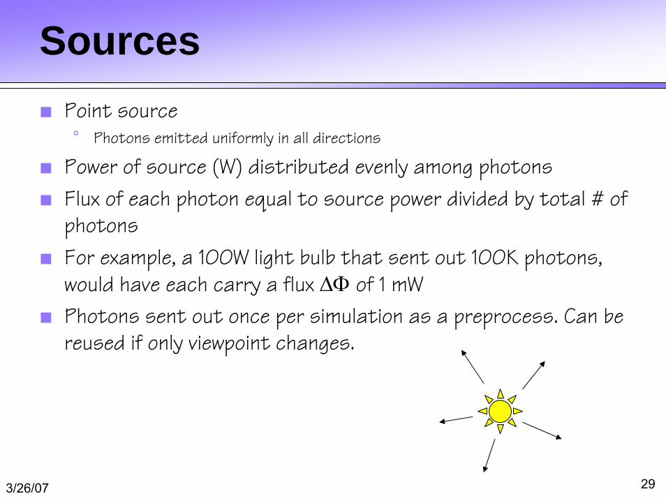
Sources Point source

° Photons emitted uniformly in all directions

Power of source (W) distributed evenly among photons

Flux of each photon equal to source power divided by total # of photons

For example, a 100W light bulb that sent out 100K photons,

would have each carry a flux ∆Φ of 1 mW

Photons sent out once per simulation as a preprocess. Can be reused if only viewpoint changes.

3/26/07 30

Russian Roulette Arvo & Kirk, SIGGRAPH90

Reflected flux only a fraction of incident flux. We could attenuate the flux of our photon based on the reflectance coefficient, and send it off in a random direction. After several reflections, spending a lot of time keeping track of very little flux

Instead, completely absorb some photons and completely reflect others at full power. Spend time tracing fewer full power photons. Probability of

reflectance is the reflectance ρ. Probability of absorption is 1 – ρ.

ρ = 60%

?

3/26/07 31

Mixed Surfaces If surfaces have specular and diffuse components

° ρd – diffuse reflectance

° ρs – specular reflectance

° ρd + ρs < 1 (conservation of energy)

Let ζ be a uniform random value from 0 to 1

If ζ < ρd then reflect diffuse (send off in a random direction)

Else if ζ < ρd + ρs then reflect specular (send off *near* reflected direction)

Otherwise absorb

ρd = 50%ρs = 30%

3/26/07 32

Storing Photons Uses a Kd-tree – (axis-aligned variant of BSP tree)

° 2-D partitions are lines

° 3-D partitions are planes

Axis of partitions alternates wrt depth of the tree

Average access time is O(log n)

Worst case O(n) when tree is severely lopsided

Need to maintain a balanced tree, which can be done in O(n log n)

Can find k nearest neighbors in O(k + log n) time using a heap

3/26/07 33

Reflected Radiance Recall the reflected radiance equation

Convert incident radiance into incident flux

Reflected radiance in terms of incident flux

Numerically

∫Ω

⋅= iiiirirrr dNLfL ωωωωωω ))(,(),(),( xx

iii

iiii dAdN

dLωωωω

)(),(),(

2

⋅Φ

=xx

∫Ω

Φ=

i

iirirrr dA

dfL ),(),(),(2 ωωωω xx

∑=

∆Φ∆

≈n

ppprprrr f

AL

1),(),(1),( ωωωω xx

∆A = πr2

3/26/07 34

How Many Photons? How big is the disk radius r ?

Large enough that the disk surrounds the n nearest photons.

The number of photons used for a radiance estimate n is usually between 50 and 500.

Radiance estimate using 50 photons

Radiance estimate using 500 photons

∆A = πr2

3/26/07 35

Filtering Too few photons cause blurry results

Simple averaging produces a box filtering of photons

Photons nearer to the sample should be weighted more heavily

Results in a cone filtering of photons

∑=

∆Φ⎟⎟

⎠

⎞

⎜⎜

⎝

⎛ −−

−≈

n

pppprpr

p

krr f

krrL

12

32

),(),(1)1(

1),( ωωωπ

ω xxx

x

3/26/07 36

Multiple Photon Maps Global L(S|D)*D photon map

° Photon sticks to diffuse surface andbounces to next surface (if it survives Russian roulette)

° Photons don’t stick to specular surfaces

Caustic LSS*D photon map° High resolution

° Light source usually emits photons only in directions that hit the objectcreating the caustic

Caustic mapphotons

Global mapphotons

3/26/07 37

Rendering Rendered by glossy-surface

distributed ray tracing

When ray hits first diffuse surface…

° Compute reflected radiance of caustic map photons

° Ignore global map photons

° Importance sample BRDF fr as usual

° Use global photon map to importance sample incident radiance function Li

° Evaluate reflectance integral by casting rays and accumulating radiances from global photon map

First diffuse intersection.

Return radiance of caustic

map photons here, but

ignore global map photons

Use global map photons to return

radiance when evaluating Li at

first diffuse intersection.

3/26/07 38

Radiosity Radiosity: Total rate of energy leaving a surface:

° Emitted

° Reflected

Model the scene as a set of patches with constant radiosity° emitters are patches too

Set up linear system

Solve

3/26/07 39

Radiosity Equation

∫+=j

jijjiiiii FABAEAB ddd ρ

Parts:° Bi: Radiosity at i

° dAi: differential area i

° Ei: emission rate at i

° ρi: reflectivity at i

° Fij: form factor

Wavelength dependence is implicit° Usually just use three (RGB)

3/26/07 40

Form Factors The form factor, Fji is the fraction of energy leaving

dAj that arrives (directly) at dAi

Form factors consider:° Distance between surfaces

° Relative Size

° Relative orientation

° Occlusion by intervening surfaces

[Draw Examples]

3/26/07 41

Discretization Discretize the scene into “patches” of constant radiosity

Reciprocity relationship of form factors [SIEG84]:

∫+=j

jjijiiiii AFBAEAB ddd ρ

∑+=j

jjijiiiii AFBAEAB ρbecomes

i

jjiij

jjiiij

AA

FF

AFAF

=

=∑+=

j ijjiii FBEB ρ

3/26/07 42

System of Equations

∑−=j

ijjii FBBE ρ

⎥⎥⎥⎥

⎦

⎤

⎢⎢⎢⎢

⎣

⎡

=

⎥⎥⎥⎥

⎦

⎤

⎢⎢⎢⎢

⎣

⎡

⎥⎥⎥⎥

⎦

⎤

⎢⎢⎢⎢

⎣

⎡

−−−

−−−−−−

nnnnnnnnn

n

n

E

EE

B

BB

FFF

FFFFFF

2

1

2

1

21

22222212

11121111

1

11

ρρρ

ρρρρρρ

What can we say about about Fii?Form factors in any row or column sum to 1 (in a closed environment)

3/26/07 43

Solving The matrix is “diagonally dominant” and Gauss-

Seidel iteration is guaranteed to converge

Solution proceeds one row at a time using estimates from previous rows

At each step the radiosity of a patch is updated based on other approximation of other patches

Emitters appear first

3/26/07 44

Rendering The radiosities are constant across the entire patch area

Simply rendering the patches produces tiled appearance

Instead interpolate radiosities to the vertices and use Gourad shading

from Baum et al. [1991]

3/26/07 45

Calculating Form Factors

2

cos cos1 ( , )d di j

i jij rx P y P

i

F V x y x yA

φ φ

π∈ ∈= ∫ ∫

Original Radiosity paper [Goral et al. 84] used analytical approach° Expensive

° Difficult to incorporate occlusion

Common techniques:° Hemicube

° Ray casting

3/26/07 46

Form factor between two polygons (actually just a part of it)

3/26/07 47

Hemicube Dispenses with outer integral (assumes little variation over i)

Uses fact that projection of surface onto bounding volume has same form factor as original surface

Surround the center of patch i with a pixelated half cube

Precompute form factor of each “pixel”

Rasterize the scene onto the faces of the hemicube

Form factor approximated asthe sum form factors of eachpixel it covers

3/26/07 48

Hemicube Limitations Aliasing

Occlusion close to surface

Close surfaces (why?)

Light sources (why?)

3/26/07 49

Ray casting Compute point to patch form factor analytically

Use raytracing to determine visibility factor

Generally, less efficient than hemicube