Global Electricity Network Feasibility Study fileIntroduction Yan ZHANG (on behalf of Dr. Jun YU)...

Presented by C1.35 members

Paris – 28 August 2018

Global Electricity NetworkFeasibility Study

� Introduction�Data collection�Methodology and modeling�Results of the simulations�Disclaimer and recommendations�Conclusion

Table of contents

IntroductionYan ZHANG

(on behalf of Dr. Jun YU)

Global Electricity Network - Feasibility Study

CIGRE Paris Session 2018 – 28 August 2018

4

The challenges

Resource shortages

� Disasters like photochemical

smog

� Acid rain and ammonia

pollution.

Environmental pollution

� Global warming

Climate change

The large-scale utilization of fossil energy

has resulted in a series of prominent problems

Oil, 110yrs28%

Natual Gas, 54yrs20%

Coal, 53yrs52%

Proven reserve of fossil fuels

� Occasional resource

shortages

� Fluctuating energy market

5

The challenges

2010 2020 2030 2040 2050

Global energy consumption continues to growGlobal energy consumption continues to grow

� It is estimated that the total global energy consumption will

reach 30 billion tons of coal equivalent in 2050.

� Getting the access to sustainable energy for everyone is a great

challenge.

30 Billion

6

Clean Energy and Interconnection

Load Centers

Wind Energy

Solar Energy

CLEAN ENERGY

• Uneven distribution

• Geographical inconsistency with load

centers

• Enormous amount

7


INTERCONNECTION

• Supports a balanced coordination of power supply of

all interconnected countries.

• Enables clean energy transmission

• Take advantage of diversity of clean energy.

Increase clean energy consumption

8


To make use of the

diversity of consumption

load patterns

To take advantage of the

high potential RES basins in

the world

To decrease the reserve

capacity in each region by

pooling reserves across

regions.

Other highlights of interconnectionOther highlights of interconnection

9

Term of Reference and Scope of C1.35

Scope of the WG:To carry out the first known feasibility study for the concept of aglobal electricity network.

The study has to

• Examine technical challenges, potential benefits, economic viability fitting with

global energy policies and environmental impact.

• Adopt one reference long term scenario for consumption and supply volumes.

• Cover now and the year 2050.

Data and scenario 2050

(External sources)

Simulations(CIGRE C1.35)

Which interconnections?

(CIGRE C1.35)

Data collectionGérald SANCHIS



11

91

2

13

11

12

10

4

5

6

7

8

3

Input data for electricity generation : forecast by 2050

Source: World Energy Council (WEC) hypothesis on generation and demand (C1.35 model with

13 regions).

6671 TWh

2438 GW

2740 TWh

904 GW 2427 TWh

912 GW

552 TWh

231 GW

4481 TWh

1534 GW

2108 TWh

644 GW

10408 TWh

3106 GW

959 TWh

398 GW

1860 TWh

763 GW

551 TWh

198 GW

2215 TWh

982 GW4885 TWh

1413 GW

2050

39850 TWh

13500 GW

WEC2013

WEC2016

44%

demand

RES53%

WEC provided annual data.

12

Input data for electricity demand by 2050

13

11

5

6

7

8

CIGRE C1.35 survey for present load patterns (source 2015&2016)

3

10

91

2 12

4

Same time reference: UTC time

1, North America2, South America3, Oceania4, North East Asia5, South East Asia6, Central Asia7, South Asia8, Middle East9, Europe10, UPS11, North Africa12, Africa13, Atlantic North

13

13

11

5

6

7

8

3

10

91

2 12

4

��

��

��

��

��

��

��

��

��

Demand pattern 2016 - Worldwide

1, North America 37%

2, Latin America 12%

3, Oceania 14%

4, East Asia 38%

5, South As ia 18%

6, North West As ia 12%

7, South West Asia 12%

8, Middle East 62%

9, Europe 26%

10, UPS 32%

11, North Africa 26%

12, Afri ca 6%

� Comparison of the Max monthly value / min monthly value (Max-min/min)

Season effect

��

��

��

��

��

��

14

Demand pattern 2016 – North -America

15

World weather databasedeveloped and maintained by NASA at 0.5x0.625 latitude/longitude spatial resolution

Taking into accountconstructive parameters(PV panel and windturbine).

RES Potential – Load Factor Estimation

16

Interconnections selectedSelection by CIGRE C1.35: • in order to limit the simulation cases -> 20 interconnections,• Preferential paths, taking into account the topography, the present grid and the RES potential.

OHL USC

AC 400 0 1%

DC 41400 7550 99%

85% 15%

17

Interconnections selected

91

2

13

11

12

10

4

5

6

7

8

3

110

OHL-DC 400 km, USC-DC 700 km

OHL-DC 1700 km

20 interconnections, mainly DC links, and Over-Head-Line technology.

1, North America2, South America3, Oceania4, North East Asia5, South East Asia6, Central Asia7, South Asia8, Middle East9, Europe10, UPS11, North Africa12, Africa13, Atlantic North

OHL USC

AC 400 0 1%

DC 41400 7550 99%

85% 15%

18

Unit costsGeneration

Source: after IEA, EIA, IRENA

Production

WACC 7%

Coût CO2 (€/t) 110

CAPEX invest

(€/kW)

fixed OPEX (%

CAPEX/yr)

life

duration

(years)

variable

cost except

CO2

(€/MWh)

CO2

emissions

(t/MWh)

fixed annual

costs

(k€/MW/yr)

variable

cost

(€/MWh)

Hydro 2 300 1,1% 80 0 0 187 0

Biomass 2 441 2,9% 30 49 0 268 49

Nuclear 3 644 1,8% 60 10 0 325 10

Coal CCS 3 804 1,5% 40 15 0,080 342 24

Wind 836 2,5% 25 0 0 93 0

Solar PV 448 1,0% 25 0 0 43 0

CCGT-CCS 1 475 1,5% 30 36 0,037 141 40

CCGT 700 1,5% 30 36 0,370 67 77

OCGT 505 1,2% 30 45 0,469 47 97

19

Unit costsGrid technology

Example:

1000 km, 1GW

360 M€ < OHL-DC < 650 M€

158M€ 158M€

1450 M€ < USC-DC < 2200 M€

Cost DC OHL DC USC AC OHL AC USC AC/DCAC/AC Back to

Back

(M€/km/GW) (M€/km/GW) (M€/km/GW) (M€/km/GW) 2 Converters 2 Substations

(M€) (M€)

Maxi 0,33 1,9 0,25 2,24 316 316

min 0,18 1,27 0,13 1,12 180 180

Source: EU projects

20

Interconnection costs(option min cost M€/GW)

91

2

13

11

12

10

4

5

6

7

8

3

110

486

Methodology and modeling

Marc LE DU



22

Key ideas

� The value of transmission grids is strongly linked to the economy of power generation mix

� Orders of magnitude :� Power generation ~ 1 000 M€/GW� Transmission line ~ 1 M€/GW/km

� 1 GW power generation ~ 1 000 km transmission lines

� The most expensive part of electric systems is the power generation � it is worth investing in transmission as much as it helps reducing the generation costs

23

Basics of power generation mix for conventional power plants

� For a given load curve to be satisfied, and assuming the grid is a copper plate, the aim is to find the “optimal” power generation mix

� “Optimal” power generation mix :� Objective : minimizes the total cost of generation : CAPEX, fixed OPEX,

variable OPEX� Constraints : balance production and demand on ever y time step.

24

Total cost of generation

� A trade off between fixed costs (CAPEX and fixed OPEX) and variable costs (variable OPEX) must be found

Cost for 1 MW generation(€)

Fixed costs (€/MW/yr)• CAPEX• Fixed OPEX

Variable costs(€/yr)

Production duration (h/yr)

Unit Variable costs (€/MWh)

Annualized

Depends on :• Investments• Life duration• WACC (interest rate)• Operation & Maintenance costs

Depends on :• Efficiency• Fuel costs• CO2 costs

25

Optimal power generation mix

� The choice between base, semi-base or peak generation plants depends on the plant load factor …

� … the plant load factor depends on the load curve

Load(GW)

Unitgeneration

costs

h/yr

h/yr

Monotonic load

to be supplied

x GW base plants

y GW semi-base plants

z GW peak plantsThis power generation mix leads to the minimum total costfor this load curve(under specific assumptions)

26

Limits of rough methods …

�Using monotonic loads for dimensioning power generation mix is limited to strong assumptions :� Dispatchable plants (no run-of-river production suc h as wind,

solar, hydro, …)� No dynamic constraints : no links between the produ ction of 2

time steps �� no storage, …� Copper-plate grid� …

� If this assumptions are not met, numerical methods are required � ANTARES tool for example

27

Antares a software developed by RTE to simulate balance between supply & demand

� Modeling of hourly scenarios of demand, capacity factors for wind, solar, hydro, etc., availability of power plants, …

� For each hourly scenario, ANTARES optimizes the investments and the unit commitment in order to meet the demand at the lowest cost.

Takes into account the capacity of

interconnections and the flows

between zones.

28

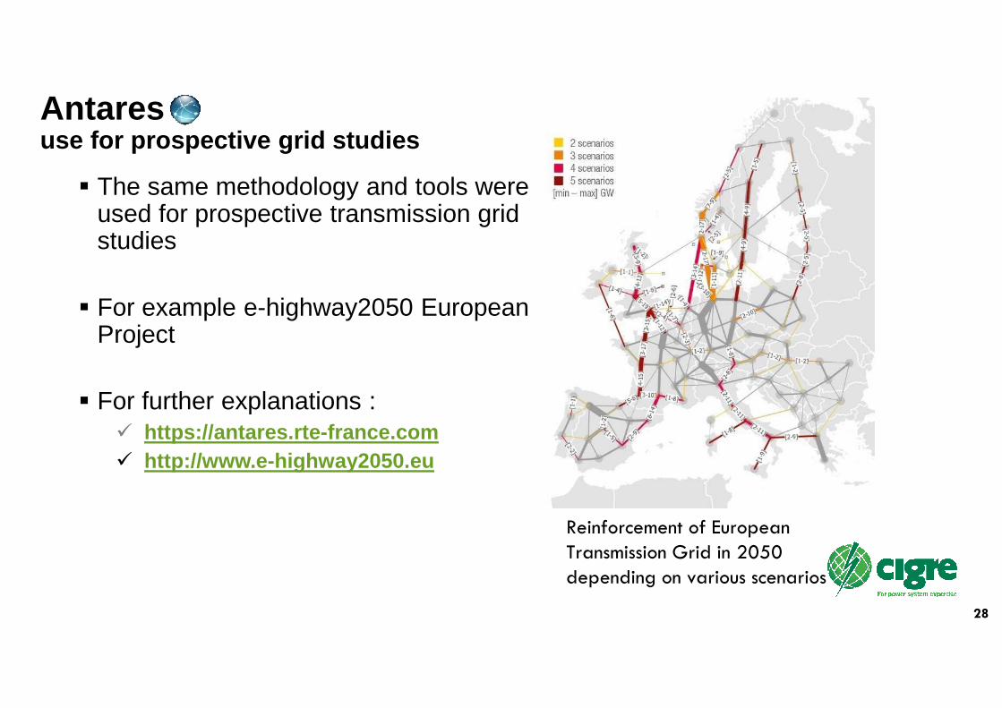
Antares use for prospective grid studies

� The same methodology and tools were used for prospective transmission grid studies

� For example e-highway2050 European Project

� For further explanations :� https://antares.rte-france.com� http://www.e-highway2050.eu

Reinforcement of European Transmission Grid in 2050 depending on various scenarios

29

11 Study cases

� 11 study cases to analyse the value of interconnections and the sensitivity to different factors

Production

capacity case

#

IntercoWind &

Solar CFstorage

CO2

(€/t)Comment/rationale

imposed optimized costs losses

According

to WEC :

- Nuclear

- Coal +

CCS

- Hydro

- Biomass

Existing

wind & PV

CCGT+CCS

CCGT

OCGT

New

Wind &PV

0 No interco Nominal None 110 Base case

1 Ref Y Nominal None 110 value of interco

1 bis Ref YModified

4&6None 110 influence of CF

2 Ref No Nominal None 110 influence of losses

3 Max Y Nominal None 110 Influence of grid cost

4 Ref Y NominalDaily - low

power110

influence of storage5 Ref Y Nominal

Daily - high

power110

6 Ref Y Nominal Seasonal 110

7 Ref Y Nominal None 30 influence of CO2 price

None

PV only 8 Ref Y Nominal None -Would it even be possible

?PV +

Wind9 Ref Y Nominal None -

Results of the simulations

Marc LE DU & Spyros CHATZIVASILEIADIS



31

Recall of major hypothesis

• The 13 zones are seen internally as “copper-plates”, i.e. there is no need of further internal reinforcements to exploit the new interconnections; this is also based on the selection of proper terminal points for each interconnection

• The unit costs for production are the same worldwide.

• There are no limits on the capacities for production or for interconnections.

32

#0 : no interconnection

For each of the 13 isolated zones :

• nuclear, Coal-CCS, hydro and biomass are imposed according to WEC scenario hypothesis

• Gas technologies (CCGT-CCS, CCGT, OCGT), wind and solar are optimized to minimize the total cost.

Production

capacity case

#

IntercoWind &

Solar CFstorage

CO2

(€/t)comment


According

to WEC :

- Nuclear

- Coal +

CCS

- Hydro

- Biomass

Existing

solar & PV

CCGT+CC

S

CCGT

OCGT

Solar PV

Wind

0 No interco Nominal None 110 reference system cost


1 bis Ref YModified



3 Max Y Nominal None 110 Influence grid cost


power110


Daily - high

power110



None


?PV +


33


91

2 12

4

5

7

8

Energy Production shares (the surface is proportional to the production)

10

Hydro

Nuclear

Coal-CCS

Wind

Solar

Gas

Biomasse

34


91

2

13

11

12

4

5

6

7

8

3

Installed capacities (GW)

913

513

682

224

196

123121

110

107

166

1183

970

246

233

177

69

49

48

34

657

502

412

267

239

314

300

360

162

61

139

92

67

55

284

239

242

0

0

0

10

WindSolar

Gas

35


0 2 000 4 000 6 000 8 000 10 000 12 000

Hydro

Biomasse

Nuclear

Coal CCS

Wind

Solar PV

CCGT-CCS

CCGT

OCGT

Production (TWh)0 500 1 000 1 500 2 000 2 500 3 000 3 500 4 000

Hydro

Biomasse

Nuclear

Coal CCS

Wind

Solar PV

CCGT-CCS

CCGT

OCGT

Installed capacity (GW)

� Total cost = 54 €/MWh (70% fixed costs, 30% variable costs)

� RES share = 53%

� CO2 emissions = 850 Mt/yr

23%38%

77%62%

Production capacity : 13 500 GW Production volumes : 39 850 TWh

0 200 400 600 800

Hydro

Biomasse

Nuclear

Coal CCS

Wind

Solar PV

CCGT-CCS

CCGT

OCGT

Costs/yr (G€)

Fixed

Variable

Annual costs : 2 150 G€

41%

59 %

Interconnection : 0 GW / 0 G€

36

#1 : reference case with interconnections

Production

capacity case

#

IntercoWind &

Solar CFstorage

CO2

(€/t)comment


According

to WEC :

- Nuclear

- Coal +

CCS

- Hydro

- Biomass

Existing

solar & PV

CCGT+CC

S

CCGT

OCGT

Solar PV

Wind



1 bis Ref YModified





power110


Daily - high

power110



None


?PV +


• Nuclear, Coal-CCS, hydro and biomass are imposed according to WEC scenario hypothesis for each zone

• Gas technologies, wind and solar PV are optimized together with the interconnexions to minimize the total cost

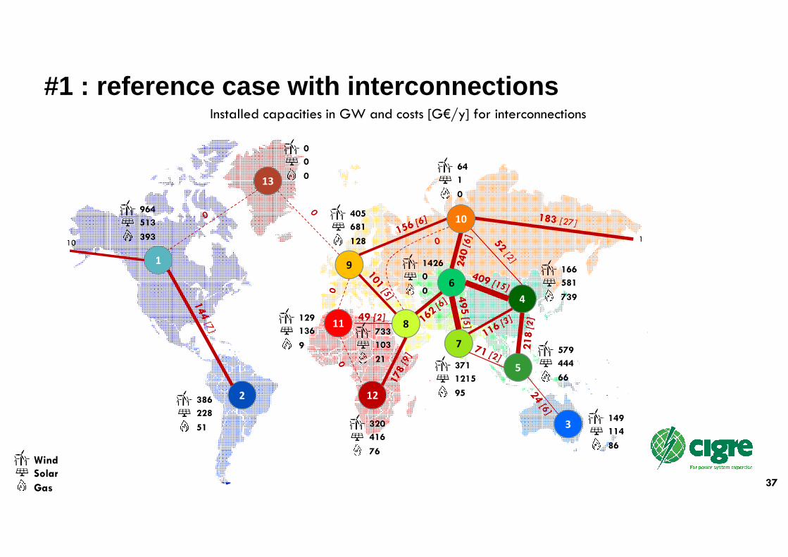
37


91

2

13

11

12

4

5

6

7

8

3

110

49 [2]

Installed capacities in GW and costs [G€/y] for interconnections

964

513

393

386

228

51149

114

86

166

581

739

579

444

66

1426

0

0

371

1215

95

733

103

21

405

681

128

64

1

0

129

136

9

320

416

76

0

0

0

WindSolar

Gas

10

38


0 200 400 600 800

Hydro

Biomasse

Nuclear

Coal CCS

Wind

Solar PV

CCGT-CCS

CCGT

OCGT

costs (G€)

no interco

with interco

0 5 000 10 000 15 000 20 000

Hydro

Biomasse

Nuclear

Coal CCS

Wind

Solar PV

CCGT-CCS

CCGT

OCGT

Production (TWh)

no interco

with interco

0 2 000 4 000 6 000

Hydro

Biomasse

Nuclear

Coal CCS

Wind

Solar PV

CCGT-CCS

CCGT

OCGT


no interco

with interco

� Total cost = 48 €/MWh (-6 €/MWh)� RES share = 76 % (+23 %)� CO2 emissions = 343 Mt/yr (-510)

Prod capacity : 14 920 GW (+1 400) Prod volumes : 40 300 TWh (+440)

Annual costs : 1 820 G€ (-330)

Overall Interconnections : 2 600 GW / 104 G€/yr

More wind

& solar PV

Less gas

… at a lower

cost

39

#1 : reference case with interconnectionsMain results

• 2 600 GW of interconnections are developed (17% of total production capacity)

• These interconnections allow for an increase of wind & solar PV production, replacing an important part of base and semi-base gas production.

– The total cost of the system goes from 54 to 48 €/MWh

– The RES part is increased (53% to 76%)

– The CO2 emissions go down

• The main interconnections capacities are developed around Central Asia, due to

– Good wind capacity factor in Central Asia (40%) and solar capacity factors in South and South-East Asia

– Close to large demand regions : North-East Asia and South-Asia

• Some interconnections possibilities are nor used at all :

– Interconnections to North Atlantic (Greenland)

– Interconnections between North Africa and Europe

– Interconnections between North Africa and the rest of Africa

• Despite its cost, the interconnections between North America and Russia is developed, used in bothdirections and allowing for a connection between Americas and the rest of the world

40

#1bis : modified capacity factors

• As the wind capacity factor in Central Asia has a big influence on the results of case #1, a sensitivity study is achieved :

– Wind capacity factor in Central Asia : 40% � 31%

– Wind capacity factor in North East Asia : 20% � 23%

Production

capacity case

#

IntercoWind &

Solar CFstorage

CO2

(€/t)comment


According

to WEC :

- Nuclear

- Coal +

CCS

- Hydro

- Biomass

Existing

solar & PV

CCGT+CC

S

CCGT

OCGT

Solar PV

Wind



1 bis Ref YModified





power110


Daily - high

power110



None


?PV +


41


91

2

13

11

12

4

5

6

7

8

3

110

964

570

435

397

235

34152

115

86

334

503

666

1055

662

3

900

0

0

287

1154

189

777

19

0

376

700

126

235

1

0

187

183

0

363

406

75

0

0

0

10

87 [3]

WindSolar

Gas


42


0 200 400 600

Hydro

Biomasse

Nuclear

Coal CCS

Wind

Solar PV

CCGT-CCS

CCGT

OCGT

costs (G€)

reference #1

Modified wind CF

0 5 000 10 000 15 000 20 000

Hydro

Biomasse

Nuclear

Coal CCS

Wind

Solar PV

CCGT-CCS

CCGT

OCGT

Production (TWh)

reference #1

Modified wind CF

0 2 000 4 000 6 000 8 000

Hydro

Biomasse

Nuclear

Coal CCS

Wind

Solar PV

CCGT-CCS

CCGT

OCGT


reference #1

Modified wind CF

� Total cost = 49 €/MWh (+1 €/MWh)� RES share = 75 % (-1 %)� CO2 emissions = 330 Mt/yr (-23)

Prod capacity : 15 300 GW (+ 400) Prod volumes : 40 220 TWh (-80)

Annual costs : 1 860 G€ (+40)

Overall Interconnections : 2 560 GW (-40) / 96 G€/yr (-8)

More wind

capacity

For a lower

production

And an

increased cost

43

#1bis : modified capacity factorsMain results

• Modifying the wind capacity factors in central Asia (40% to 31%) and Northern Asia (20% to 23%) does not change the global view of installed capacities for production and interconnections.

• However it modifies the location of production and interconnections

– Less wind capacities are developed in Central Asia (but they remain very high)

– Replaced by more wind and solar capacities in South-East Asia (good capacity factors for both production)

– The big interconnections capacity between North East Asia and Central Asia is replaced by the same level of interconnections between North East Asia and South East Asia.

44

#3 : high cost of interconnections

• We use maximum instead of minimum values of interconnections unit costs

Production

capacity case

#

IntercoWind &

Solar CFstorage

CO2

(€/t)comment


According

to WEC :

- Nuclear

- Coal +

CCS

- Hydro

- Biomass

Existing

solar & PV

CCGT+CC

S

CCGT

OCGT

Solar PV

Wind



1 bis Ref YModified





power110


Daily - high

power110



None


?PV +


45


91

2

13

11

12

4

5

6

7

8

3

110

917

940

558

329

163

44124

110

104

248

628

742

718

475

76

1213

0

0

291

991

152

369

553

177

232

1

14

129

126

13

333

360

113

0

0

0

10

41 [3]

644

191

45

WindSolar

Gas


46


0 200 400 600

Hydro

Biomasse

Nuclear

Coal CCS

Wind

Solar PV

CCGT-CCS

CCGT

OCGT

costs (G€)

reference #1

Max cost of interco

0 5 000 10 000 15 000 20 000

Hydro

Biomasse

Nuclear

Coal CCS

Wind

Solar PV

CCGT-CCS

CCGT

OCGT

Production (TWh)

reference #1

Max cost onf interco

0 2 000 4 000 6 000

Hydro

Biomasse

Nuclear

Coal CCS

Wind

Solar PV

CCGT-CCS

CCGT

OCGT


reference #1

Max cost of interco

� Total cost = 50 €/MWh (+ 2 €/MWh)� RES share = 73 % (-3 %)� CO2 emissions = 444 Mt/yr (+101)

Prod capacity : 14 790 GW (-140) Prod volumes : 40 127 TWh (-172)

Annual costs : 1 880 G€ (+60)

Overall Interconnections : 1 911 GW (-687) / 106 G€/yr (+2)

less wind and

solar PV

More gas

… at a higher

cost

47

#3 : high cost of interconnectionsMain results

• Increasing the costs of interconnections leads to lower their development : 1900 GW instead of 2600 GW (-26%) for the same cost

– It concerns all the interconnections, especially the longer ones : the interconnection between North America and Russia goes from 161 to 41 GW

• The interconnection level still remains high (12% of the production capacities).

• The total system cost is a bit higher (from 48 to 50 €/MWh).

• As the production is more local, more gas is needed, which impacts the CO2 emissions and the RES share.

48

#4 & 5 : Daily storage

• The sensitivity of a daily storage is simulated, assuming that 10% of energy of the daily demand in each zone could be moved within the day, with an efficiency of 90%. Two kinds of “flexibility” are simulated

– Case #4 “low power” storage : the ratio energy/power of the storage is 5 h

– Case #5 “high power” storage : the ratio energy/power of the storage is 1 h

• No cost hypothesis is taken : we assume the storage is “for free”

Production

capacity case

#

IntercoWind &

Solar CFstorage

CO2

(€/t)comment


According

to WEC :

- Nuclear

- Coal +

CCS

- Hydro

- Biomass

Existing

solar & PV

CCGT+CC

S

CCGT

OCGT

Solar PV

Wind



1 bis Ref YModified





power110


Daily - high

power110



None


?PV +


49

#5 : Daily storage – high power

91

2

13

11

12

4

5

6

7

8

3

110

827

979

272

351

378

0153

168

33

166

758

449

221

1322

14

1318

0

0

444

1908

0

560

479

0

504

214

83

1

1

0

116

127

3

318

469

21

0

0

0

10

24 [11]

WindSolar

Gas


50

#5 : Daily storage – high power

0 200 400 600

Hydro

Biomasse

Nuclear

Coal CCS

Wind

Solar PV

CCGT-CCS

CCGT

OCGT

costs (G€)

reference #1

Daily storage - high power

0 5 000 10 000 15 000 20 000

Hydro

Biomasse

Nuclear

Coal CCS

Wind

Solar PV

CCGT-CCS

CCGT

OCGT

Production (TWh)

reference #1


0 2 000 4 000 6 000 8 000

Hydro

Biomasse

Nuclear

Coal CCS

Wind

Solar PV

CCGT-CCS

CCGT

OCGT


reference #1


� Total cost = 46 €/MWh (- 2 €/MWh)� RES share = 80 % (+4 %)� CO2 emissions = 222 Mt/yr (-121)

Prod capacity : 15 765 GW (+837) Prod volumes : 40 681 TWh (+382)


Overall Interconnections : 2 632 GW (+34) / 88 G€/yr (-16)

More solar PV

Less wind & gas

51

#4 : Daily storage – low power

0 200 400 600

Hydro

Biomasse

Nuclear

Coal CCS

Wind

Solar PV

CCGT-CCS

CCGT

OCGT

costs (G€)

reference #1

Daily storage - low power

0 5 000 10 000 15 000 20 000

Hydro

Biomasse

Nuclear

Coal CCS

Wind

Solar PV

CCGT-CCS

CCGT

OCGT

Production (TWh)

reference #1


0 2 000 4 000 6 000 8 000

Hydro

Biomasse

Nuclear

Coal CCS

Wind

Solar PV

CCGT-CCS

CCGT

OCGT


reference #1


� Total cost = 47 €/MWh (- 1 €/MWh)� RES share = 78 % (+3 %)� CO2 emissions = 277 Mt/yr (-66)

Prod capacity : 14 828 GW (-100) Prod volumes : 40 506 TWh (+207)


Overall Interconnections : 2 537 GW (-61) / 102 G€/yr (-2)

52

#4 & 5 : Daily storageMain results • Considering a possible daily storage does not change the global level of interconnection

• However it changes the repartition and the location of production

– Daily storage promotes Solar PV production, replacing partly wind and gas production, specially for “high power” storage

– Depending on the location, this leads to :

• Lower interconnection capacities, where they were due to wind productions

• Higher interconnection capacities for links between North East Asia and South & South East Asia, with a big development or solar capacities in those two regions

– The increase of capacity on these two interconnections compensates the lower capacities elsewhere.

• The results are sensitive to the “power” of the storage : to promote the solar PV, a high power is required

– For low power daily storages, the development of solar PV is not enough to significantly modify the interconnections level.

53

#8 : Solar PV Only

• As a very theoretical test, we try to design the production and interconnexions system if the only production source allowed was solar PV.

Production

capacity case

#

IntercoWind &

Solar CFstorage

CO2

(€/t)comment


According

to WEC :

- Nuclear

- Coal +

CCS

- Hydro

- Biomass

Existing

solar & PV

CCGT+CC

S

CCGT

OCGT

Solar PV

Wind



1 bis Ref YModified





power110


Daily - high

power110



None


?PV +


54

#8 : Solar PV Only

9

13

11

12

5

6

7

8

3

110

261 [10]

0

16 840

0

14 2480

19 093

0

537

0

2127

0

495

0

4 908

0

992

0

1 099

0

6

0

778

0

777

0

0

10

2

1

4

WindSolar

Gas


55

#8 : Solar PV OnlyMain results

• The “solar PV only” case study leads to huge levels of

– production capacities : 62 000 GW are installed (more than 4 times the capacities of reference case #1)

• The capacities are installed worldwide, with big capacities in Oceania, North America and Latin America, to get the benefits of both seasonal and daily complementarity of productions

– Interconnections : 24 000 GW worldwide (38% of production capacities – 45% of system costs)

0

5

10

15

20

25

TWh

Hourly production & load

Prod totale Conso totale

• This leads to 97 000 TWh of production

– including 57 000 TWh of spillage (52 000 TWh) and losses (5 000 TWh), to satisfy a 40 000 TWhload

• The total system cost is 120 €/MWh

– compared to 48 €/MWh for reference case #1

Production

Load

56

#9 : Solar PV + wind Only

• Same as 8, but for solar PV + wind as candidates for production

Production

capacity case

#

IntercoWind &

Solar CFstorage

CO2

(€/t)comment


According

to WEC :

- Nuclear

- Coal +

CCS

- Hydro

- Biomass

Existing

solar & PV

CCGT+CC

S

CCGT

OCGT

Solar PV

Wind



1 bis Ref YModified





power110


Daily - high

power110



None


?PV +


57

#9 : Solar PV + wind Only

9

13

11

12

5

6

7

8

3

110

1 530

1 017

833

987337

384

512

1 791

1 644

515

1 616

0

1 007

1 341

2 053

0

1 260

1 529

1 760

0

1 480

1 187

601

852

1 334

0

10

2

1

4

849 [31]

WindSolar

Gas


58

#9 : “Solar PV + wind”Main results

• Compared to the “solar PV only” case #8, this case study shows the complementarity of wind and solar, thanks to the interconnections.

• It leads to :

– 26 000 GW production capacities : 16 000 GW for wind + 10 000 GW for solar PV

– 7 800 GW of interconnections (30% of production capacities – 18% of system costs) : all interconnections are used, with very big capacities around Central Asia and Middle East

• The production is still very high : 62 000 TWh

– including 22 000 TWh of spillage (21 300 TWh) and losses (700 TWh), for a 40 000 TWhload

• The total system cost is more acceptable : 58 €/MWh

– compared to 48 €/MWh for reference case #1

– and compared to 54 €/MWh for base case #00

5

10

15

20

25

TWh

Hourly production and load

Prod totale Conso totale

Production

Load

Disclaimer and recommendations

Antonio ILICETO



60

Disclaimer: limits of this concept-study

• The limits of the pre-feasibility study:– Few electrical nodes, rough model, the uncertainties, ….

– Political/social barriers to intercontinental interconnections are not taken into account. • They require mutual trust, and reliance on each other’s support during scarcities, as well as trading rules. Trust

and trading rules are pre-requisites for the large investments in interconnections that the study suggests wouldbenefit the world.

• The realisation of such global interconnection woul d heavily depend on:– Assessing technical, environmental and economic viability (inside this study, at preliminar level) – Consolidating assumptions and evaluation models to be shared and agreed both locally and globally – Assessing operational issues and interoperability– Assessing financial viability and construction challenges (project finance and project management)– Setting up legislation & regulation frameworks necessary to authorise, own, build and operate such

interconnections– Envisaging market rules and business models for the most efficient exploitation of the interconnections

61

Recommendations for further analysis and studies

� Which interconnection should start the process?‒ While detecting the main trends, these preliminary results should pave the way

for further analysis, for consolidating the assumptions and for identifying the most promising steps of a global network.

� Trade-off between alternative solutions (storage, de mand-response, price elasticity,…) and transmission ‒ the present study focuses mostly on the trade-off between transmission and

generation.

ConclusionGérald Sanchis



63

�Global Electricity Interconnection is an ambitious concept.�WG C1.35 is finalising the first known quantitative feasibility

study for the concept of a global electricity network. It has provided a possible geographical and technical configuration and preconditions for its feasibility considering technology and economical aspects.

� Future work and possible follow-up.

Conclusion

Copyright © 2018

This tutorial has been prepared based upon the work of CIGRE and its Working Groups. If it is used in total or in part, proper reference and credit should be given to CIGRE.

Disclaimer notice

“CIGRE gives no warranty or assurance about the contents of this publication, nor does it accept any responsibility, as to the accuracy or exhaustiveness of the information. All implied warranties and conditions are excluded to the maximum extent permitted by law”.

Copyright & Disclaimer notice

Global Electricity Network Feasibility Study fileIntroduction Yan ZHANG (on behalf of Dr. Jun YU)...

Documents

Transcript of Global Electricity Network Feasibility Study fileIntroduction Yan ZHANG (on behalf of Dr. Jun YU)...