Global Currency Hedging

JOHN Y. CAMPBELL, KARINE SERFATY-DE MEDEIROS, AND

LUIS M. VICEIRA∗

Journal of Finance forthcoming

ABSTRACT

Over the period 1975 to 2005, the US dollar (particularly in relation to the Cana-

dian dollar) and the euro and Swiss franc (particularly in the second half of the

period) have moved against world equity markets. Thus these currencies should be

attractive to risk-minimizing global equity investors despite their low average returns.

The risk-minimizing currency strategy for a global bond investor is close to a full cur-

rency hedge, with a modest long position in the US dollar. There is little evidence

that risk-minimizing investors should adjust their currency positions in response to

movements in interest differentials.

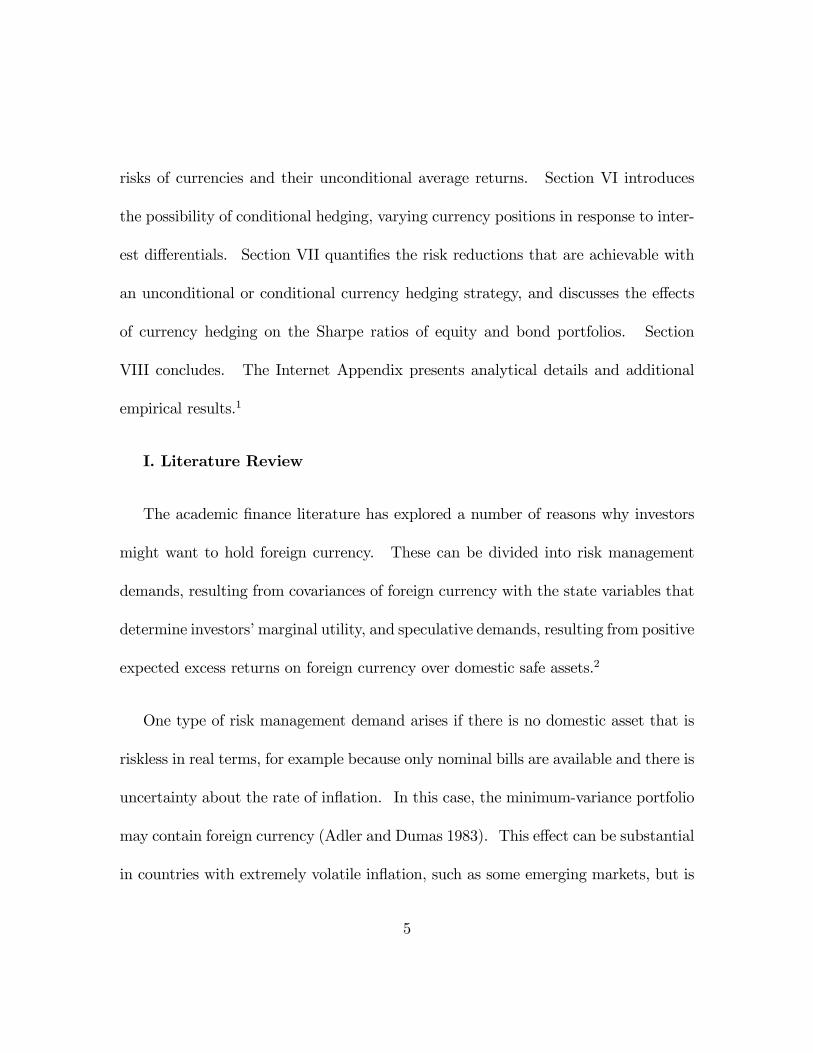
What role should foreign currency play in a diversi�ed investment portfolio? In

practice, many investors appear reluctant to hold foreign currency directly, perhaps

because they see currency as an investment with high volatility and low average re-

turn. At the same time, many investors hold indirect positions in foreign currency

when they buy foreign equities or bonds without hedging the currency exposure im-

plied by the foreign asset holding. Such investors receive the foreign-currency excess

return on their foreign assets, plus the return on foreign currency.

In this paper we consider an investor with an exogenous portfolio of equities or

bonds and ask how the investor can use foreign currency to manage the risk of the

portfolio. We assume that the investor�s domestic money market is riskless in real

terms, and use mean-variance analysis to �nd the foreign currency positions that

minimize the risk of the total portfolio. We consider seven major developed-market

currencies, the dollar, euro, Japanese yen, Swiss franc, pound sterling, Canadian

dollar and Australian dollar, over the period 1975 to 2005. Any of these can be the

investor�s domestic currency or can be available as a foreign currency. We assume a

one-quarter investment horizon, but obtain similar results for horizons ranging from

one month to one year.

Although our framework is standard, and has been applied to US holdings of for-

1

eign currencies by Glen and Jorion (1993), our implementation and empirical results

are novel in several respects. Following Glen and Jorion, we start by considering

an equity investor who chooses �xed currency weights to minimize the unconditional

variance of her portfolio. Such an investor wishes to hold currencies that are nega-

tively correlated with equities. Our �rst novel result is that our seven currencies fall

along a spectrum. At one extreme, the Australian dollar and the Canadian dollar are

positively correlated with local-currency returns on equity markets around the world,

including their own domestic markets. At the other extreme, the euro and the Swiss

franc are negatively correlated with world stock returns and their own domestic stock

returns. The Japanese yen, the British pound, and the US dollar fall in the middle,

with the yen and the pound more similar to the Australian and Canadian dollars,

and the US dollar more similar to the euro and the Swiss franc.

When we consider currencies in pairs, we �nd that risk-minimizing equity investors

should short those currencies that are more positively correlated with equity returns

and should hold long positions in those currencies that are more negatively correlated

with returns. When we consider all seven currencies as a group, we �nd that optimal

currency positions tend to be long the US dollar, the Swiss franc, and the euro, and

short the other currencies. A long position in the US-Canadian exchange rate is a

particularly e¤ective hedge against equity risk.

2

We obtain a second novel result when we consider the risk-minimization problem

of global bond investors rather than global equity investors. We �nd that most

currency returns are almost uncorrelated with bond returns and thus risk-minimizing

bond investors should avoid holding currencies; that is, they should fully currency-

hedge their international bond positions. This is consistent with common practice

of institutional investors, although global bond mutual funds are available with or

without currency hedging. The US dollar is an exception to the general pattern

in that it tends to appreciate when bond prices fall, that is when interest rates rise,

around the world. This generates a modest demand for US dollars by risk-minimizing

bond investors.

In capital market equilibrium, one might expect that average currency returns

would re�ect the risk characteristics of currencies. Speci�cally, if reserve currencies

are attractive to risk-minimizing global equity investors, these currencies might o¤er

lower returns in equilibrium. We analyze the historical average returns on currency

pairs and obtain a third novel result, that high-beta pairs have delivered higher aver-

age returns. However the historical reward for taking equity beta risk in currencies

has been quite modest, and much smaller than the historical average excess return

on a global stock index.

3

Another way to �nd a risk-return relation in foreign currencies is to condition

upon currency characteristics that are known to predict currency returns, and to

ask whether these characteristics predict currency risks. Following an extensive

literature on the predictive power of interest di¤erentials for currency returns, we

use deviations of interest di¤erentials from their time-series averages as conditioning

variables, imposing that they have the same e¤ects on currency covariances regardless

of the particular currency pair under consideration. Our fourth novel result is that

increases in interest rates have only modest e¤ects on currency-equity covariances.

Over the full sample period, and particularly the �rst half of the sample, increases in

interest di¤erentials are, if anything, associated with decreases in these covariances.

This implies that risk-minimizing equity investors should tilt their portfolios towards

currencies that have temporarily high interest rates, amplifying the speculative �carry

trade�demands for such currencies rather than o¤setting them.

The organization of the paper is as follows. Section I sets the stage by brie�y

reviewing the related literature. Section II describes our data and conducts prelimi-

nary statistical analysis of stock, bond, and currency returns. Section III lays out the

analytical framework we use for our empirical analysis and presents unconditionally

optimal currency hedges for equity portfolios, while Section IV reports the analogous

results for bond portfolios. Section V discusses the relation between unconditional

4

risks of currencies and their unconditional average returns. Section VI introduces

the possibility of conditional hedging, varying currency positions in response to inter-

est di¤erentials. Section VII quanti�es the risk reductions that are achievable with

an unconditional or conditional currency hedging strategy, and discusses the e¤ects

of currency hedging on the Sharpe ratios of equity and bond portfolios. Section

VIII concludes. The Internet Appendix presents analytical details and additional

empirical results.1

I. Literature Review

The academic �nance literature has explored a number of reasons why investors

might want to hold foreign currency. These can be divided into risk management

demands, resulting from covariances of foreign currency with the state variables that

determine investors�marginal utility, and speculative demands, resulting from positive

expected excess returns on foreign currency over domestic safe assets.2

One type of risk management demand arises if there is no domestic asset that is

riskless in real terms, for example because only nominal bills are available and there is

uncertainty about the rate of in�ation. In this case, the minimum-variance portfolio

may contain foreign currency (Adler and Dumas 1983). This e¤ect can be substantial

in countries with extremely volatile in�ation, such as some emerging markets, but is

5

quite small in developed countries over short time intervals. Campbell, Viceira,

and White (2003) show that it can be more important for investors with long time

horizons, because nominal bills subject investors to �uctuations in real interest rates,

while nominal bonds subject them to in�ation uncertainty which is relatively more

important at longer horizons. If domestic in�ation-indexed bonds are available,

however, they are riskless in real terms if held to maturity and thus drive out foreign

currency from the minimum-variance portfolio.

Another type of risk management demand for foreign currency arises if an in-

vestor holds other assets for speculative reasons, and foreign currency is correlated

with those assets. For example, an investor may wish to hold a globally diversi�ed

equity portfolio. If the foreign-currency excess return on foreign equities is negatively

correlated with the return on the foreign currency (as would be the case, for example,

if stocks are real assets and the shocks to foreign currency are primarily related to

foreign in�ation), then an investor holding foreign equities can reduce portfolio risk by

holding a long position in foreign currency. This type of risk management currency

demand is the subject of this paper.

Many international investors think not about the foreign currency positions they

would like to hold, but about the currency hedging strategy they should follow.3

6

An unhedged position in international equity, for example, corresponds to a long

position in foreign currency equal to the equity holding, while a fully hedged position

corresponds to a net zero position in foreign currency. When currencies and equities

are uncorrelated, risk management demands for foreign currencies are zero, implying

that in the absence of speculative demands, full hedging is optimal (Solnik 1974).

Empirically, Perold and Schulman (1988) �nd that US investors can reduce volatility

by fully hedging the currency exposure implicit in internationally diversi�ed equity

and bond portfolios.

We derive optimal hedging strategies for global equity and bond investors. Like

Glen and Jorion (1993), we �nd that optimal currency hedging substantially reduces

risk for equity investors. The bene�ts of optimal hedging are large even in countries

like Canada where full hedging is actually riskier than no hedging at all. We report

results for quarterly returns, but these results are robust to variation in the investment

horizon between one month and one year. Froot (1993) studies the dollar and the

pound over a longer sample period and �nds that risk-minimizing foreign currency

positions increase with the investment horizon, implying that long-horizon equity

investors should not hedge their currency risk. We do not �nd this horizon e¤ect in

our post-1975 dataset.

7

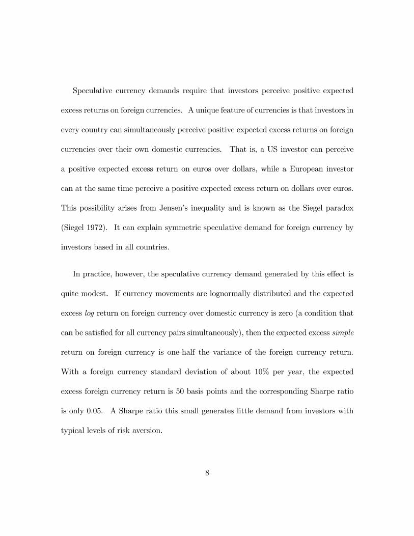
Speculative currency demands require that investors perceive positive expected

excess returns on foreign currencies. A unique feature of currencies is that investors in

every country can simultaneously perceive positive expected excess returns on foreign

currencies over their own domestic currencies. That is, a US investor can perceive

a positive expected excess return on euros over dollars, while a European investor

can at the same time perceive a positive expected excess return on dollars over euros.

This possibility arises from Jensen�s inequality and is known as the Siegel paradox

(Siegel 1972). It can explain symmetric speculative demand for foreign currency by

investors based in all countries.

In practice, however, the speculative currency demand generated by this e¤ect is

quite modest. If currency movements are lognormally distributed and the expected

excess log return on foreign currency over domestic currency is zero (a condition that

can be satis�ed for all currency pairs simultaneously), then the expected excess simple

return on foreign currency is one-half the variance of the foreign currency return.

With a foreign currency standard deviation of about 10% per year, the expected

excess foreign currency return is 50 basis points and the corresponding Sharpe ratio

is only 0.05. A Sharpe ratio this small generates little demand from investors with

typical levels of risk aversion.

8

A more important source of speculative currency demand arises from expected

excess returns on particular currencies, as opposed to all currencies simultaneously.

Although unconditional average excess returns on currencies are close to zero, there

is evidence that conditional expected excess returns on currencies undergo short-term

�uctuations which constitute the basis for active currency strategies. Most obviously,

the literature on the forward premium puzzle (Hansen and Hodrick 1980, Fama 1984,

Hodrick 1987, Engel 1996) shows that currencies with high short-term interest rates

deliver high returns on average. The currency carry trade, which exploits this phe-

nomenon by holding high-rate currencies and shorting low-rate currencies, was ex-

tremely pro�table in and beyond our sample period until 2008 (Burnside et al. 2007,

Brunnermeier, Nagel, and Pedersen 2008).

It is natural to ask whether the carry trade has risk characteristics that o¤set its

pro�tability. Farhi and Gabaix (2008) argue that high-rate currencies are exposed to

the risk of rare economic disasters, while Lustig and Verdelhan (2007) �nd that high-

rate currencies, in a sample that includes emerging-market currencies, have higher

sensitivity to US consumption growth. We use sensitivity to world stock returns as

a measure of risk, and �nd that developed-market currencies with high unconditional

average interest rates do have somewhat higher betas with the world stock market,

but that there is no tendency for a currency whose interest rate is temporarily high to

9

have a temporarily higher beta. Over our full sample period and in the �rst half of

the sample, currency betas even have a weak tendency to decline when interest rates

increase. Thus risk considerations might deter equity investors from implementing

an unconditional form of the carry trade, but a conditional form of the trade, that

invests in currencies with temporarily high interest rates, should be attractive even

to risk-averse equity investors.

II. Data and Summary Statistics

Our empirical analysis uses stock return data from Morgan Stanley Capital Inter-

national, and data on exchange rates, short-term interest rates, and long-term bond

yields from the International Financial Statistics database published by the Inter-

national Monetary Fund.4 We calculate log bond returns from yields on long-term

bonds using the approximation suggested in Campbell, Lo and MacKinlay (1997).5

These data series are available at a monthly frequency, and we report results for sev-

eral di¤erent investment horizons in the appendix, but our basic analysis assumes a

one-quarter horizon and therefore runs monthly regressions of overlapping quarterly

excess returns. We report results for seven developed economies: Australia, Canada,

Euroland, Japan, Switzerland, the UK and the US. The sample period starts in

1975:7, the earliest date for which we have data available for all variables and for all

10

seven markets, and ends in 2005:12.

We de�ne �Euroland�as a value-weighted stock basket that includes Germany,

France, Italy, and the Netherlands. These are the countries in the euro zone for

which we have the longest record of stock total returns, interest rates, and exchange

rates. For simplicity, we will refer to the Euroland stock portfolio as a �country�

stock portfolio when describing our empirical results, even though this is not literally

correct. With regard to currencies, prior to 1999 we refer to a basket of currencies

from those countries, with weights given by their relative stock market capitalization,

as the �euro�.

Of course, our de�nition of Euroland implies some look-ahead bias, since in 1975

it would not have been obvious whether a European monetary union would occur,

and which countries from the region would have been part of that union. However,

one can reasonably argue that these countries would have been candidates, and that

from the perspective of today�s investors, it probably makes sense to consider these

markets as a single market. We have also conducted our analysis including only

Germany in Euroland, and using the deutschemark to proxy for the euro before 1999;

this procedure gives very similar results.

Table I reports the full-sample annualized mean and standard deviation of short-

11

term nominal interest rates, log stock and bond returns in excess of their local short-

term interest rates, changes in log exchange rates with respect to the US dollar, and

log currency excess returns with respect to the dollar. The means of log excess

returns (geometric averages) are adjusted for Jensen�s Inequality by adding one half

their variance to convert them into mean simple excess returns (arithmetic averages).

Annualized average nominal short-term interest rates di¤er across countries. They

are lowest for Switzerland and Japan, and highest for Australia, Canada, and the UK.6

Short-term rates exhibit very low annualized volatility, under 2% for all countries.

Average changes in exchange rates with respect to the US dollar over this period

are negative for the Australian dollar, close to zero for the Canadian dollar, the

British pound, and the euro, and positive for the Swiss franc and the yen, re�ecting

an appreciation of these currencies with respect to the US dollar over this period.

Exchange rate volatility relative to the dollar is in the range 10-13% for all currencies

except the Canadian dollar, which moves closely with the US dollar giving a bilateral

volatility of only 5.4%.

Excess returns to currencies are small on average and exhibit annual volatility

similar to that of exchange rates, a result of the stability of short-term interest rates.

Using the usual formula for the mean of a serially uncorrelated random variable, it is

12

easy to verify that unconditional mean excess returns on currencies are insigni�cantly

di¤erent from zero.

Table II reports full-sample quarterly correlations of foreign-currency excess re-

turns (Panel A), and fully currency-hedged excess returns on stocks (Panel B) and

bonds (Panel C). For simplicity, we report in Panel A the average correlation of

each currency pair across all possible base currencies in our set, giving results for

individual base currencies in the appendix. Panel A shows that all currency returns

are positively cross-correlated. Currency correlations are large� almost all correla-

tion coe¢ cients are above 30%� but they are far from perfect, implying that there is

signi�cant cross-sectional variation in the dynamics of exchange rates.

Four correlations stand out as unusually large. The Canadian dollar exhibits a

very high correlation with the US dollar (89%) and also with the Australian dollar

(70%). The high correlation of the Canadian dollar with both the US dollar and

the Australian dollar re�ects the dual role of the Canadian economy as a resource-

dependent economy that is simultaneously highly integrated with the US. Similarly,

the euro is highly correlated with the Swiss franc (89%) and to a lesser extent the

British pound (68%), re�ecting the integration of European economies. Importantly,

these correlations are high not only on average, but also individually, regardless of

13

the base currency used to measure them.

The correlation coe¢ cients between stock market returns shown in Panel B are all

between 40% and 70%, with two important exceptions. The Canadian stock market

is highly correlated with the US stock market (75%), and the Swiss stock market is

highly correlated with the Euroland stock market (80%). The Canadian stock market

also exhibits a relatively large correlation of 66% with the Australian stock market.

These correlations demonstrate again the dual role of the Canadian economy and the

integration of the Swiss economy with the European economy.

While signi�cant, the stock market correlations are still small enough to suggest

the presence of substantial bene�ts of international diversi�cation in this sample pe-

riod. Not surprisingly, the Japanese stock market exhibits the lowest cross-sectional

correlation with all other markets. This is a re�ection of the prolonged period of low

or negative stock market returns in Japan during the 1990�s, at a time when most

other markets delivered large positive returns.

Long-term bond market correlations are generally somewhat smaller than stock

market correlations. Panel C in Table III shows that, with some important exceptions,

these correlations are all in the range of 30-60%. The exceptions are the Euroland

bond market, which is highly correlated with both the Swiss bond market (65%)

14

and the US bond market (62%), and the Canadian bond market, which is highly

correlated with the US bond market (79%). Overall, these results imply that there

are meaningful bene�ts to international diversi�cation in bond market investing.

III. Unconditional Currency Risk Management for Equity Investors

A. Estimating Unconditional Currency Demands

Our empirical analysis is based on the estimation of risk-minimizing currency de-

mands for a set of stock and bond portfolios and currencies. We begin by establishing

some notation. We use Rc;t+1 to denote the gross return in currency c from holding

country c assets from the beginning to the end of period t + 1, and !c;t to denote

the weight of those assets at time t in the investor�s portfolio. Sc;t+1 denotes the spot

exchange rate in units of domestic currency per unit of foreign currency c at the end

of period t+1, and Ic;t denotes the nominal short-term nominal interest rate on bills

denominated in currency c.

By convention, we index the domestic country by c = 1 or d and the n foreign

countries by c = 2; :::; n + 1. Of course, the domestic exchange rate is constant over

time and equal to 1: S1;t+1 = 1 for all t: For convenience, throughout this section we

set the domestic country to be the US, and hence refer to the domestic investor as a

US investor, and to the domestic currency as the dollar. We also use small caps to

15

denote log (or continuously compounded) returns, exchange rates, and interest rates.

That is, rc;t+1 = log(Rc;t+1), sc;t+1 = log(Sc;t+1), and ic;t = log(1 + Ic;t)

An investor holding an arbitrary portfolio of domestic and foreign assets can alter

the currency exposure of her portfolio by overlaying a zero investment portfolio of

domestic and foreign bills or, equivalently, by entering into an appropriate number

of forward currency contracts. This is intuitive. Since the investor is already fully

invested in other assets, she can alter the currency exposure implied by those assets

only by borrowing� or equivalently, by shorting bonds� in some currencies, and using

the proceeds to buy bonds denominated in other currencies.

For convenience we work with net currency exposures relative to full currency

hedging, which we denote by c;t, instead of currency hedging demands. Of course,

there is direct correspondence between them: c;t = 0 corresponds to a fully hedged

currency position, in which the investor does not hold any exposure to currency c.

A positive value of c;t means that the investor holds exposure to currency c, or

equivalently that the investor does not fully hedge the currency exposure implicit

in her stock position in country c. When c;t = !c;t, the portfolio is completely

unhedged.

The internet appendix shows that with arbitrary currency exposure, the log port-

16

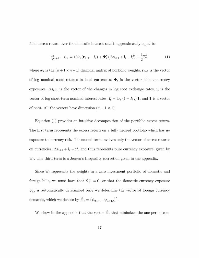
folio excess return over the domestic interest rate is approximately equal to

rhp;t+1 � i1;t = 10!t (rt+1 � it) +0

t

��st+1 + it � idt

�+1

2�ht ; (1)

where !t is the (n+1�n+1) diagonal matrix of portfolio weights, rt+1 is the vector

of log nominal asset returns in local currencies, t is the vector of net currency

exposures, �st+1 is the vector of the changes in log spot exchange rates, it is the

vector of log short-term nominal interest rates, idt = log (1 + I1;t)1, and 1 is a vector

of ones. All the vectors have dimension (n+ 1� 1).

Equation (1) provides an intuitive decomposition of the portfolio excess return.

The �rst term represents the excess return on a fully hedged portfolio which has no

exposure to currency risk. The second term involves only the vector of excess returns

on currencies, �st+1 + it � idt , and thus represents pure currency exposure, given by

t. The third term is a Jensen�s Inequality correction given in the appendix.

Since t represents the weights in a zero investment portfolio of domestic and

foreign bills, we must have that 0t1 = 0, or that the domestic currency exposure

1;t is automatically determined once we determine the vector of foreign currency

demands, which we denote by et =� 2;t; :::; n+1;t

�0:

We show in the appendix that the vector et that minimizes the one-period con-

17

ditional global variance of the log excess return on the hedged portfolio is equal to

e�RM;t = �Vart

�f�st+1 +eit �eidt��1 hCovt �10!t (rt+1 � it) ;�f�st+1 +eit �eidt��i ;(2)

where we have added the subscript RM to emphasize that equation (2) describes risk

management currency demands. In the rest of the paper we will refer to this risk

management component of currency demand simply as optimal currency demand or

currency exposure.

Equation (2) writes e�RM;t as a vector of multiple regression coe¢ cients of portfoliostock returns on currency returns. If stock returns and exchange rates are uncorre-

lated, the risk management currency demand is zero. In this case holding currency

exposure adds volatility to the investor�s portfolio and, unless this volatility is com-

pensated, the investor is better o¤holding no currency exposure at all or, equivalently,

fully hedging her portfolio. If stock returns and exchange rates are positively cor-

related, the foreign currency tends to depreciate when the stock market falls. Thus

the investor can reduce portfolio return volatility by over-hedging, that is, by short-

ing foreign currency in excess of what would be required to fully hedge the currency

exposure implicit in her stock portfolio. Conversely, a negative correlation between

stock returns and exchange rates implies that the foreign currency appreciates when

18

the stock market falls. Then the investor can reduce portfolio return volatility by

under-hedging, that is, by holding foreign currency.

A useful property of the optimal currency demands in (2), proven in the appendix,

is that for a given stock portfolio, they are invariant to changes in the base currency,

provided that a riskless real asset is available in each base currency and that the set of

available currencies (which always includes an investor�s own domestic currency) does

not change. If we restrict the set of available currencies to a pair, for example the

US dollar and the euro, this means that residents of both the US and Germany will

have the same optimal demands for dollars and euros corresponding to a given equity

portfolio. Residents of a third country, however, have another domestic currency

available to them and so they will not necessarily have the same demands for dollars

and euros even if they hold the same equity portfolio. If we allow a larger set of

available currencies, then residents of all the countries in the set will have the same

vector of optimal currency demands for a given equity portfolio.

In this section and the next we present estimation results which are based on an

unconditional version of equation (2). The unconditional version of our model follows

immediately from the conditional version by simply assuming constant risk premia

and constant second moments of returns. We relax this assumption in section VI,

19

which examines conditional hedging policies where the covariances of portfolio returns

with currency excess returns vary over time as a function of interest rate di¤erentials.

Equation (2) with constant second moments implies that we can compute opti-

mal currency exposures by regressing portfolio excess returns 10!t(rt+1 � it) onto a

constant and the vector of currency excess returns f�st+1 �eidt +eit, and switching thesign of the slopes. In our empirical analysis we consider several practically relevant

cases. First, we consider an investor who is fully invested in a domestic stock portfolio

and optimally decides how much exposure to a single currency c to hold in order to

minimize total portfolio return volatility. The optimal currency demand is the nega-

tive of the slope coe¢ cient in a regression of the domestic excess stock return onto a

constant and the excess return on currency c.

Second, we consider an investor who is fully invested in a domestic stock portfolio,

but who uses the whole range of available currencies to minimize total portfolio return

volatility. In that case the vector of optimal currency demands is given by the negative

of the slopes of a multiple regression of the excess stock return on the domestic market

onto a constant and the vector of currency excess returns.

Third, we consider a case where the investor holds an equally weighted global

equity portfolio, using the whole vector of available currencies to minimize total port-

20

folio return volatility. Finally, in the appendix we also consider value weighted and

home biased global equity portfolios.

B. Single-Country Stock Portfolios

We start our empirical analysis by examining the case of an investor who is fully

invested in a single-country equity portfolio and is considering whether exposure to

other currencies would help reduce the volatility of her quarterly portfolio return.

Table III reports optimal currency exposures for the case in which the investor is

considering one currency at time (Panel A), and that in which she is considering mul-

tiple currencies simultaneously (Panel B). In both panels, the reference stock market

is reported at the left of each row, while the currency under consideration is reported

at the top of each column. In all tables we report Newey-West heteroskedasticity and

autocorrelation consistent standard errors in parentheses below each optimal currency

exposure. Following standard convention, we mark with one, two, or three stars co-

e¢ cients for which we reject the null of zero at a 10%, 5%, and 1% signi�cance level,

respectively.

Panel A in Table III considers an investor who is deciding how much to hedge of

the currency exposure implicit in an investment in a speci�c national stock market, in

isolation from other investments and currencies this investor might hold. To facilitate

21

interpretation, it is useful to discuss an example in detail. The �rst non-empty cell in

the �rst column of the table, which corresponds to the Australian stock market and

the euro, has a value of 0.39. This means that a risk-minimizing Euroland investor

who is fully invested in the Australian stock market and has access to the Australian

dollar and the euro should buy a portfolio of euro-denominated bills worth 1.39 euros

per euro invested in the Australian stock market, �nancing this long position with a

short position in Australian bills� i.e., by borrowing Australian dollars. That is, the

investor should over-hedge the Australian dollar exposure implicit in her Australian

stock market investment, and hold a net long 39% exposure to the euro.

Panel A of Table III shows that optimal demands for foreign currency are large,

positive and statistically signi�cant for two stock markets (rows of the table), those

of Australia and Canada. Investors in the Australian and Canadian stock markets

are keen to hold foreign currency, regardless of the particular currency under consid-

eration, because the Australian and Canadian dollars tend to depreciate against all

currencies when their stock markets fall; thus any foreign currency serves as a hedge

against �uctuations in these stock markets. The long positions in euros, Swiss francs,

or US dollars are particularly large and statistically signi�cant.

At the opposite extreme, it is optimal for investors in the Swiss stock market to

22

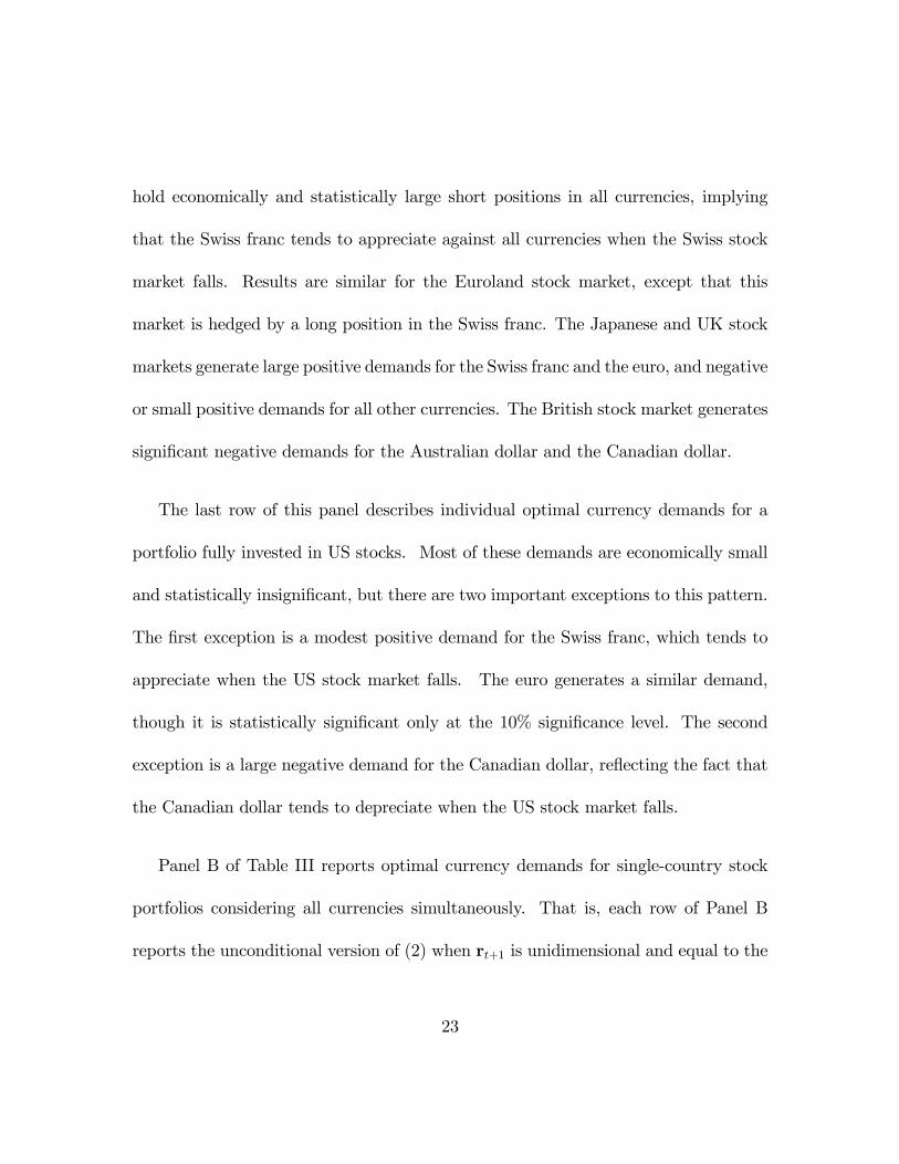
hold economically and statistically large short positions in all currencies, implying

that the Swiss franc tends to appreciate against all currencies when the Swiss stock

market falls. Results are similar for the Euroland stock market, except that this

market is hedged by a long position in the Swiss franc. The Japanese and UK stock

markets generate large positive demands for the Swiss franc and the euro, and negative

or small positive demands for all other currencies. The British stock market generates

signi�cant negative demands for the Australian dollar and the Canadian dollar.

The last row of this panel describes individual optimal currency demands for a

portfolio fully invested in US stocks. Most of these demands are economically small

and statistically insigni�cant, but there are two important exceptions to this pattern.

The �rst exception is a modest positive demand for the Swiss franc, which tends to

appreciate when the US stock market falls. The euro generates a similar demand,

though it is statistically signi�cant only at the 10% signi�cance level. The second

exception is a large negative demand for the Canadian dollar, re�ecting the fact that

the Canadian dollar tends to depreciate when the US stock market falls.

Panel B of Table III reports optimal currency demands for single-country stock

portfolios considering all currencies simultaneously. That is, each row of Panel B

reports the unconditional version of (2) when rt+1 is unidimensional and equal to the

23

stock market shown on the leftmost column. Note that the the numbers in each row

must add up to zero, since the domestic currency exposure must o¤set the vector of

foreign currency demands.

When single-country stock market investors consider investing in all currencies

simultaneously, they almost always choose positive exposures to the US dollar, the

euro and the Swiss franc, and negative exposures to the Australian dollar, Canadian

dollar, British pound, and Japanese yen. Relative to panel A, the optimal currency

demands are generally larger and statistically more signi�cant for the US dollar, and

less statistically signi�cant for the euro and the Swiss franc. This re�ects two features

of the multiple-currency analysis. First, a position that is long the US dollar and

short the Canadian dollar is a highly e¤ective hedge against stock market declines.

Thus allowing investors to use both North American currencies increases the risk

management demand for the US dollar. Second, the euro and Swiss franc are both

good hedges but they are highly correlated; thus the demand for each currency is less

precisely estimated when investors are allowed to take positions in both currencies.

In this sense the euro and the Swiss franc are substitutes for one another.

C. Global Equity Portfolios

Thus far we have considered only investors who are fully invested in a single

24

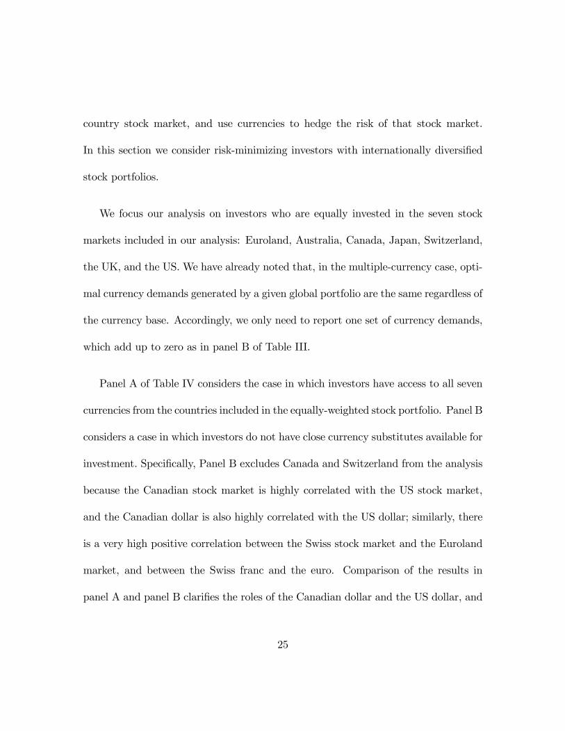
country stock market, and use currencies to hedge the risk of that stock market.

In this section we consider risk-minimizing investors with internationally diversi�ed

stock portfolios.

We focus our analysis on investors who are equally invested in the seven stock

markets included in our analysis: Euroland, Australia, Canada, Japan, Switzerland,

the UK, and the US. We have already noted that, in the multiple-currency case, opti-

mal currency demands generated by a given global portfolio are the same regardless of

the currency base. Accordingly, we only need to report one set of currency demands,

which add up to zero as in panel B of Table III.

Panel A of Table IV considers the case in which investors have access to all seven

currencies from the countries included in the equally-weighted stock portfolio. Panel B

considers a case in which investors do not have close currency substitutes available for

investment. Speci�cally, Panel B excludes Canada and Switzerland from the analysis

because the Canadian stock market is highly correlated with the US stock market,

and the Canadian dollar is also highly correlated with the US dollar; similarly, there

is a very high positive correlation between the Swiss stock market and the Euroland

market, and between the Swiss franc and the euro. Comparison of the results in

panel A and panel B clari�es the roles of the Canadian dollar and the US dollar, and

25

the euro and the Swiss franc, in investors�portfolios. Both panels report estimates of

optimal currency demands based �rst on our full sample, and then on two subperiods,

1975 to 1989 (Subperiod I) and 1990 to 2004 (Subperiod II). We discuss subperiod

results in part D of this section.

The optimal currency portfolio in Panel A has a large, statistically signi�cant

exposure of 40% to the US dollar, and an even larger negative exposure of -61% to

the Canadian dollar. These two positions are not independent of each other: Panel B

shows that, once we exclude the Canadian dollar from the menu of currencies available

to the investor, the optimal exposure to the US dollar becomes small and statistically

insigni�cant. Just as in the previous analysis of single-country stock portfolios, a

position that is long the US dollar and short the Canadian dollar helps investors

hedge against global stock market movements. The 3-month annualized return on

this position, driven by the movements of the bilateral US/Canadian exchange rate, is

plotted in Figure 1 together with the 3-month annualized excess return on the equally

weighted, fully currency-hedged global equity index. The �gure clearly shows the

tendency of the US dollar to appreciate relative to the Canadian dollar in periods of

stock market weakness.

The optimal currency portfolio in Panel A also has positive exposures to the euro

26

and the Swiss franc. These exposures are not economically very large individually,

and statistically signi�cant only at a 10% level. This lack of individual economic and

statistical signi�cance is because the euro and the Swiss franc are close substitutes.

Panel B shows that when the Swiss franc is excluded from the menu of currencies, the

demand for the other currency in the pair, the euro, increases dramatically to 56%

and is statistically signi�cant at the 1% level. Figure 2 plots the 3-month annualized

return of the euro against an equally weighted basket of other currencies, together

with the currency-hedged excess global equity return.

In addition to the optimal negative exposure to the Canadian dollar already dis-

cussed, the optimal exposures to the Australian dollar, the Japanese yen, and the

British pound are also negative. These short positions are small and statistically

insigni�cant for the pound, but larger and statistically signi�cant for the yen. The

Australian dollar short position is small if the Canadian dollar is included in the set of

currencies, but becomes larger and statistically signi�cant in panel B when the Cana-

dian dollar is excluded. These two currencies, which are unusually highly correlated

with one another, are substitutes in investors�currency portfolios.

Once again, it is useful to review the exact meaning of the numbers we report.

The numbers shown in Table IV are optimal currency exposures. If it is optimal for

27

all investors to fully hedge the currency exposure implicit in their stock portfolios or,

equivalently, to hold no currency exposure, the optimal currency demands shown in

Table IV should be equal to zero everywhere. To obtain optimal currency hedging de-

mands from optimal currency exposures, we need only compute the di¤erence between

portfolio weights� which in this case are 14.3% for each country stock market� and

the optimal currency exposure corresponding to that country.

The results in Panel A imply that, say, a risk-minimizing Euroland investor holding

our equally-weighted seven-country equity portfolio would invest 99 euro cents in

currencies for each euro invested in the stock portfolio. These 99 euro cents would be

invested in US Treasury bills worth 40 euro cents, Euroland (say, German) bills worth

32 euro cents, and Swiss bills worth 27 euro cents. These purchases would be �nanced

with proceeds from borrowing Australian dollars (11 euro cents per euro invested in

the stock portfolio), Canadian dollars (61 cents), yen (17 cents) and British pounds

(10 cents). Note that the similarity of the 99 euro cents invested in long and short

currency positions to the 100 euro cents invested in equities is merely an arbitrary

feature of this particular example, not a general property of the optimal hedging

strategy.

We can easily restate these results in terms of hedging demands. The Euroland

28

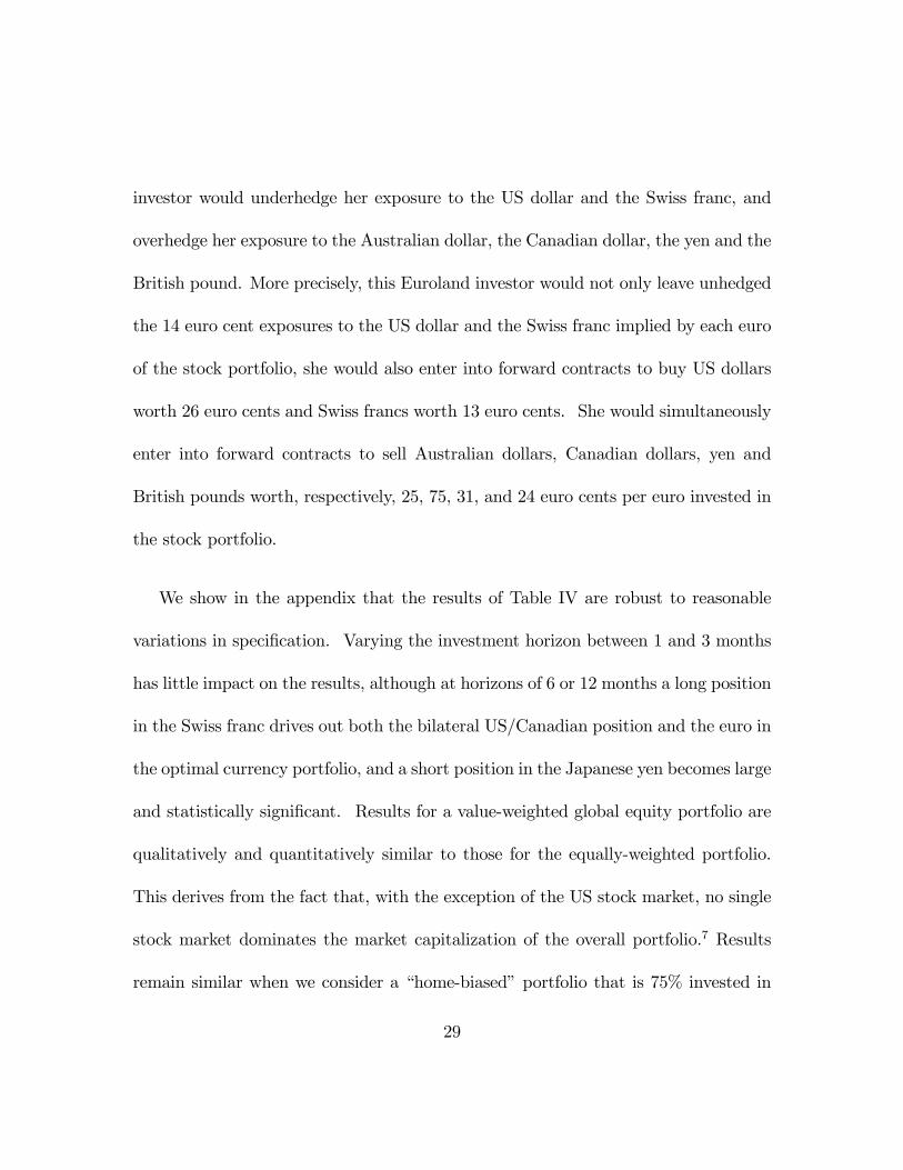
investor would underhedge her exposure to the US dollar and the Swiss franc, and

overhedge her exposure to the Australian dollar, the Canadian dollar, the yen and the

British pound. More precisely, this Euroland investor would not only leave unhedged

the 14 euro cent exposures to the US dollar and the Swiss franc implied by each euro

of the stock portfolio, she would also enter into forward contracts to buy US dollars

worth 26 euro cents and Swiss francs worth 13 euro cents. She would simultaneously

enter into forward contracts to sell Australian dollars, Canadian dollars, yen and

British pounds worth, respectively, 25, 75, 31, and 24 euro cents per euro invested in

the stock portfolio.

We show in the appendix that the results of Table IV are robust to reasonable

variations in speci�cation. Varying the investment horizon between 1 and 3 months

has little impact on the results, although at horizons of 6 or 12 months a long position

in the Swiss franc drives out both the bilateral US/Canadian position and the euro in

the optimal currency portfolio, and a short position in the Japanese yen becomes large

and statistically signi�cant. Results for a value-weighted global equity portfolio are

qualitatively and quantitatively similar to those for the equally-weighted portfolio.

This derives from the fact that, with the exception of the US stock market, no single

stock market dominates the market capitalization of the overall portfolio.7 Results

remain similar when we consider a �home-biased�portfolio that is 75% invested in

29

the domestic stock market and 25% invested in a value-weighted world portfolio that

excludes this market.

In summary, the risk-minimizing strategy for a global equity investor involves long

exposure to the US dollar and the euro (or a combination of the euro and the Swiss

franc), a large short position in the Canadian dollar, and smaller short positions in all

other major currencies. That is, investors in global equities want to underhedge their

exposure to the dollar, the euro, and the Swiss franc, and overhedge their exposure to

the other currencies. This strategy minimizes the volatility of overall portfolio returns,

because the euro, Swiss franc, and US dollar tend to appreciate when international

stock markets decline.

D. Stability Across Subperiods

The sample period for which we have estimated optimal currency exposures in-

cludes an early period of global high in�ation and interest rates, with exceptional

performance of the Japanese stock market relative to other stock markets, followed

by another subperiod of global lower in�ation and interest rates, with extremely poor

performance of the Japanese stock market. The second subperiod also saw the re-

uni�cation of Germany and the creation of the euro as a common European currency.

It is reasonable to examine if the results we have shown for the full sample hold

30

across these two markedly di¤erent subperiods, so we divide our sample period into

the periods 1975 to 1989 and 1990 to 2005.

The bottom two rows in each panel of Table IV report subsample results for an

investor holding an equally-weighted global stock portfolio, and using the vector of

available currencies to manage risk. The results are generally familiar, with long

positions for the US dollar, Swiss franc, and euro, and short positions for other

currencies. It is striking, however, that US dollar positions tend to fall between the

�rst subperiod and the second, while the sum of euro and Swiss franc positions (in

Panel A) or the euro position (in Panel B) strongly increase. The time-series plot

in Figure 2 also shows that the euro began to move more consistently against world

stock markets in the second subsample.

In summary, an important change occurred between the periods 1975 to 1989 and

1990 to 2005: The Swiss franc and the euro became much more competitive with the

US dollar as desirable currencies for risk-minimizing global equity investors. This

change is not an artefact of our use of a composite currency to proxy for the euro in

the period before the creation of a common European currency, because we obtain

similar results when we use the deutschemark as our euro proxy. Rather, it is likely

to re�ect the fact that the euro has found growing acceptance as a reserve currency

31

for international investors.

IV. Unconditional Currency Risk Management for Bond Investors

We now consider the risk-minimizing currency exposures implied by an equally-

weighted global bond portfolio. Table V, whose structure is identical to Table IV,

reports optimal currency exposures at a one-quarter horizon in the multiple currency

case for our full sample period and for the subperiods 1975 to 1989 and 1990 to 2005.

Risk-minimizing currency demands for internationally diversi�ed bond market in-

vestors are generally very small and not statistically signi�cant. The US dollar is

an exception. The optimal demand for the US dollar is positive and statistically

signi�cant, regardless of whether the dollar is the only currency available for invest-

ment, or just one of many. But these dollar exposures are economically small. They

are largest in the �rst subperiod, and almost zero in the second subperiod. Here

again we see evidence of a decline over time in the attractiveness of the US dollar for

risk-minimizing global investors.

We have also considered single-country bond portfolios. This is relevant to many

investors, since �home bond bias�is even more prevalent among investors than �home

equity bias�, and in most countries relatively few mutual funds o¤er international

bonds. The results are shown in the appendix. We �nd modest positive demands

32

for the US dollar, consistent with the results in Table V. We also �nd that an investor

holding UK bonds will hold all foreign currencies, re�ecting the fact that the British

pound tends to depreciate when the British bond market declines.

Overall, our results imply that international bond investors should fully hedge the

currency exposure implicit in their bond portfolios, with possibly a small long bias

towards the US dollar. Interestingly, full currency hedging is more common among

international bond mutual funds than among international equity funds, and is also

frequently practiced by US institutions investing in international bonds.

V. Unconditional Currency Risk and Return

In section III we showed that currencies systematically di¤er in their comovements

with global stock markets. Excess returns on reserve currencies� the US dollar, the

euro, and the Swiss franc� covary negatively with global stock market returns, while

excess returns on other currencies� particularly those of commodity-dependent Aus-

tralia and Canada� covary positively. These correlations generate positive risk man-

agement demands for reserve currencies, and negative risk management demands for

other currencies.

However, in equilibrium investors must be willing to hold all currencies (Black

1990). This suggests that average excess returns on currencies might adjust to gen-

33

erate speculative currency demands that o¤set the risk management demands we

have identi�ed. In global capital market equilibrium, investors may be willing to

receive lower compensation for holding US dollar, euro, and Swiss franc denominated

bills because of the hedging properties of these currencies, while they may demand

higher compensation for holding bills denominated in other currencies. In fact, we

saw in Table I that the US and Switzerland have had the lowest currency returns in

our sample, and together with Euroland have had the lowest interest rates with the

exception of Japan. If this is a systematic phenomenon, it suggests that a country

bene�ts from having a reserve currency not only because international demand for its

monetary base generates seigniorage revenue, but also because international demand

for its Treasury bills reduces the interest cost of �nancing the government debt.8

We now explore the equilibrium consequences of risk management demand for

currencies by looking at the relation between currencies�average excess returns and

their betas with a global stock index. We consider all possible non-redundant pairs

(or exchange rates) in our cross section of currencies, and treat each one as a long-

short portfolio of bills. For example, the excess return on the Canadian dollar with

respect to the US dollar is the return on a portfolio long Canadian bills and short US

Treasury bills.

34

For each of these portfolios, we compute the average log currency excess return

and its beta with respect to the currency-hedged excess return on a value-weighted

global stock portfolio, and we plot all these mean returns and betas together in a

single �gure.9 To simplify our plot, we choose the ordering of the pairs so that their

betas are all positive.

Figure 3 shows the mean-beta diagram based on our full sample. This �gure

plots full-sample annualized average excess currency returns on the vertical axis, and

currency betas in the horizontal axis. The points marked with triangles refer to

long-short currency portfolios with euro-denominated bills on the short side of the

portfolio. The square corresponds to the portfolio long Canadian dollars and short

US dollars, and the circles correspond to all other non-redundant currency pairs.

The �gure also plots a regression line of currency excess returns on currency betas,

with the intercept restricted to equal zero. We can interpret this line as the security

market line generated from a global CAPM using currencies as assets. The slope

of this line is 3.2%, and the R2 is reasonably large at 48%; adding a free intercept

has little e¤ect on these estimates. The slope of the security market line re�ects the

equilibrium world market premium implied by currency returns. At 3.2% per annum,

this premium is smaller than the ex-post average excess return on world stock markets

35

over this period, which Table I shows is about 7%. However, this estimate is close to

the ex-ante equity risk premium that others have estimated from US equity returns

over a longer period in which the ex-post equity premium has also been very large

(Fama and French, 2002).

The point in the �gure that lies furthest to the right corresponds to the portfolio

long Canadian dollars and short US dollars. We have shown that a position long US

dollars and short Canadian dollars is a particularly e¤ective hedge against �uctuations

in global equity markets. Conversely, a portfolio long Canadian dollars and short US

dollars is particularly risky, because it is highly positively correlated with global stock

markets. Figure 3 shows that this is the portfolio with the largest full-sample beta,

above 0.6. It provides investors with an average positive return of about 1.2% per

annum (see Table I) which, though positive, is located below the �tted security market

line and is well below the average return on other portfolios with lower betas.

We have shown that portfolios which are long euro-denominated bills also help

investors attenuate �uctuations in global stock portfolios, because the euro tends to

covary negatively with global equity returns. Conversely, portfolios which are short

euros and long other currencies are positively correlated with global equities. These

are the points corresponding to the euro pairs shown in Figure 6. As expected, these

36

portfolios all exhibit positive betas. While their average excess returns exhibit a

positive relation with betas, they tend to lie below the �tted security market line.

Overall, we do see di¤erences in average realized currency returns that correlate

with currency risks. However, these average return di¤erences are quite modest,

particularly in the case of the US dollar and the euro. Also, it is important to

keep in mind that sample average currency returns are noisy estimates of true mean

currency returns. None of the currencies in our sample have excess returns relative

to the US dollar that are signi�cantly di¤erent from zero at the 5% signi�cance level.

Figure 4 repeats the exercise shown in Figure 3, except that it treats all currency

pairs in each of the subperiods we considered in section III.D (1975 to 1989 and 1990

to 2005) as separate assets. Consistent with the results of section III.D, portfolios

which are short the euro tend to be signi�cantly riskier in the second subsample,

re�ecting the increasing tendency of the euro to move as a reserve currency. Also

consistent with our earlier results, the portfolio which is long the Canadian dollar

and short the US dollar is somewhat less risky in the second subperiod. In general,

currency pairs show a much wider dispersion in betas in the second subperiod. The

security market lines have modest positive slopes in both subperiods, but of course

the precision of mean currency return estimates is even lower in the subperiods than

37

in the full sample.

VI. Conditional Currency Risk Management

In previous sections of this paper we have estimated unconditional risk manage-

ment demands for currencies, and have found that reserve currencies tend to have

positive risk management demands and low average returns.

Along with these cross-sectional patterns, there could also be systematic variation

in currency risks over time. It is well known that interest di¤erentials predict ex-

cess returns on currencies, even controlling for cross-currency di¤erences in average

returns. Contrary to the predictions of the uncovered interest parity hypothesis,

currencies whose short-term interest rates are higher than normal tend to appreciate

relative to currencies whose short-term interest rates are lower than normal. This

behavior contributes to the pro�ts of the currency carry trade, which takes long

positions in high-interest-rate currencies and short positions in low-interest-rate cur-

rencies. Some of these pro�ts come from long-run di¤erences in average currency

returns and interest rates, of the sort summarized in Table I, but carry trade pro�ts

also result from time-variation in currency returns along with interest di¤erentials.

It is natural to ask if this conditional component of the carry trade is attractive to

risk-minimizing investors, or if such investors should avoid currencies with temporarily

38

high interest di¤erentials. To explore this question, we consider a conditional model

for risk management currency demand which depends linearly on interest di¤erentials:

e�RM;t =

e�0 ��it � idt

�+ e�

1 ��it � idt �

�it � idt

��(3)

where�it � idt

�is the unconditional expectation of the vector of interest di¤erentials,

e�0 = ( 0;2; :::; 0;n+1)

0, e�1 = ( 1;2; :::; 1;n+1)

0, and � is the element-by-element prod-

uct operator. Thus e�RM;0 �

�it � idt

�represents the vector of average risk management

demands, and e�RM;1 the vector of sensitivities of those demands to movements in

interest di¤erentials over time.

Using (2), we can estimate currency risk management demands (3) by estimating

the simple regression

10!t (rt+1 � it) = 0 �n+1Xc=2

0;c(�st+1 � idt + ic;t)�ic;t � i1;t

��n+1Xc=2

1;c(�st+1 � idt + ic;t)�ic;t � i1;t �

�ic;t � i1;t

��+ "t+1;(4)

where the left hand side variable is the excess return on a fully hedged portfolio. We

are primarily interested in estimating the vector of slopes e�1 = ( 1;2; :::; 1;n+1)

0 and

testing whether they are zero. Note that when they are zero, the regression model

(4) recovers exactly the unconditional risk management demands that we estimated

in sections III and IV.

39

We estimate two sets of conditional risk management currency demands, and re-

port the results in Table VI. First, we consider the case where only one single foreign

currency is available for investment, in addition to the domestic or base currency;

second, we consider the case where all currencies are available for investment simul-

taneously. Table VI reports results for both a global equity portfolio and a global

bond portfolio.

To increase the power of our tests, we estimate (4) imposing the constraint that

all slopes are equal, i.e., that e�1 = 11. Table VI reports the constrained estimate of

the slope 1 for each base currency, its Newey-West standard error, and the p-value

of the null hypothesis that this slope is the same across all currencies. We omit from

the table the estimated average risk management demands e�RM;0 � it � idt , because

they are very similar both economically and statistically to the unconditional risk

management demands reported in sections III and IV. It is important to note here

that the coe¢ cients 0;c and 1;c in model (3) are not invariant to the base currency

of the investor, even in the multiple currency case.10 Accordingly, we report results

for each possible base currency in the rows of the table.

The left panel of Table VI shows results for the equally-weighted global equity

portfolio. In the single-foreign-currency case, we �nd almost no evidence that risk

40

management currency demands vary with interest di¤erentials. The estimated slopes

are all positive, but they are close to zero and imprecisely estimated. In the multiple-

foreign-currency case we �nd positive and statistically signi�cant coe¢ cients whenever

the base currency is a reserve currency� the euro, the Swiss franc, or the US dollar.

The slopes are insigni�cantly di¤erent from zero for other base currencies.11

These results imply that the currency carry trade is attractive not only to currency

speculators, but also to risk-minimizing equity investors, provided that their base

currency is a reserve currency and that they can also hold �xed positions in foreign

currencies that are unrelated to interest di¤erentials. The time-series pattern shown

in Table VI, that increases in a currency�s interest rate improve its risk characteristics,

contradicts the cross-sectional pattern illustrated in Figures 6 and 7, that normally

high-rate currencies have poor risk characteristics.

Although this is a striking result, it is important not to exaggerate its signi�cance.

It applies only when the base currency is a reserve currency, and even in these cases the

e¤ect is modest. The reserve-currency slope coe¢ cients reported in Table VI are in

the range 4 to 6, which imply standard deviations of foreign currency weights of about

4-6%, given that the standard deviations of interest di¤erentials are about 1%.12 Such

standard deviations are quite small relative to the average risk management currency

41

demands reported in Table IV. Also, the appendix shows that within subsamples,

the reserve-currency slope coe¢ cients are positive and signi�cant only in the second

of our two subsamples, and only for euroland and Switzerland.

The right panel of Table VI looks at the risk-management properties of the carry

trade from the point of view of a global bond market investor. None of the slope

coe¢ cients are statistically signi�cant except for an Australian bond investor trading

in multiple currencies, who �nds that increasing interest rates make foreign currencies

riskier.

To better relate the time-series evidence to our earlier cross-sectional �ndings, we

have also estimated our unconditional risk management currency demands adding

an additional synthetic currency to the base set of currencies. Following Lustig and

Verdelhan (2007), this synthetic currency is a zero-investment portfolio of currencies

which at the start of every month in our sample period goes long an equally weighted

portfolio of the three currencies with the largest nominal short-term interest rates,

and short an equally weighted portfolio with the currencies with the smallest nominal

short-term interest rates. Thus its returns mimic one of the most popular implemen-

tations of the currency carry trade.

In the appendix, we report that the equally-weighted global equity portfolio gener-

42

ates a positive and statistically signi�cant risk management demand for the synthetic

currency when all other currencies are available for investment, but a negative and

signi�cant risk management demand when only the synthetic currency is available.

When risk-minimizing equity investors can hold �xed long positions in reserve cur-

rencies and short positions in commodity-dependent currencies, they are willing to

hold an additional position in the synthetic carry-trade portfolio, but this portfolio

is unattractive in isolation because on average it tends to short reserve currencies

and hold commodity-dependent currencies. This �nding reproduces the contrast be-

tween the cross-sectional pattern illustrated in Figure 6 and the time-series evidence

reported in Table VI.13

Table VI uses nominal interest di¤erentials, the usual basis for the carry trade,

as conditioning information. It is also possible to condition on lagged ex post real

interest di¤erentials. When we do this, in the appendix, we �nd only one case where

a risk-minimizing investor would want to condition currency demand on real interest

di¤erentials, and this case (a UK equity investor with access to multiple currencies)

again has the demand for each currency increasing in its interest di¤erential.

In conclusion, we �nd relatively weak evidence that interest di¤erentials provide

important conditioning information for currency risk management. When we allow

43

risk-minimizing positions in our seven currencies to move with interest di¤erentials,

we �nd statistically signi�cant time-variation only when the base currency is the euro,

Swiss franc, or US dollar. This time-variation is quite small relative to the uncondi-

tional average currency demands we estimated earlier. Interestingly, it increases the

demand for currencies with temporarily high interest rates, amplifying the speculative

demand rather than o¤setting it. We obtain similar results when we add a synthetic

carry-trade currency to our unconditional analysis.

VII. Risk Reduction from Currency Hedging

We have argued that �xed positions in foreign currencies, possibly with some

additional time-variation in currency positions in response to changing interest dif-

ferentials, can reduce portfolio risks for global equity and bond investors. But how

large are the feasible risk reductions?

Table VII reports the portfolio standard deviations that investors can achieve

by combining their global stock and bond portfolios with risk-minimizing currency

exposures. For each base currency, we report the annualized standard deviations

of quarterly returns given several alternative currency hedging strategies. The �rst

three columns report volatilities for unhedged, half hedged, and fully hedged portfo-

lios. Half hedging is a compromise strategy that is popular with some institutional

44

investors. Next we report the volatilities of various types of optimally hedged port-

folios. The baseline case adopts �xed, unconditionally optimal currency positions,

as in sections III and IV. We compare this with constrained conditional hedging in

the manner of Table VI. The volatilities are independent of the base currency for

the cases with full or unconditionally optimal hedging, but not for the cases with no

hedging, half hedging, or constrained conditionally optimal hedging. The right hand

part of the table reports F-statistics and p-values to test the statistical signi�cance of

the risk reductions achieved by unconditionally optimal currency hedging in relation

to full hedging and zero hedging, and by constrained conditional hedging in relation

to unconditionally optimal hedging.

Full sample results, in Table VII, show that the bene�t of full currency hedging

depends sensitively on an investor�s base currency. It is particularly large for Eu-

roland and Swiss investors, because these investors have a risk-reducing base currency

so they gain by hedging back to that currency and out of foreign currencies. The

volatility reduction from full currency hedging is particularly small for Australian

and Canadian investors, because the home currency for these investors is risky in the

sense that it is positively correlated with their equity positions. In fact, full currency

hedging actually increases risk for a Canadian investor.

45

Optimal hedging, of course, reduces risk for all investors, including Australians

and Canadians. The important point is that the bene�t of optimal hedging is sub-

stantial, both economically and statistically. The big gain comes from adopting

an unconditionally optimal currency hedging strategy with �xed currency positions.

Relative to full hedging, this strategy reduces the standard deviation of an equally-

weighted global equity portfolio by 135 basis points. This di¤erence is statistically

highly signi�cant, with p-values that are well below 1%.

There is only a small additional reduction from conditional currency hedging that

responds to time-varying interest di¤erentials. The largest additional risk reductions

come for Swiss investors (11 basis points, signi�cant at the 2% level) and Euroland and

US investors (6 basis points each, signi�cant at around the 6% level). Unconditional

hedging with a synthetic carry-trade currency delivers a comparably modest risk

reduction of 8 basis points relative to unconditionally optimal currency hedging.

The gains from currency hedging are also substantial for global bond investors,

but in this case almost all the gains can be achieved by full currency hedging. Table

VII shows that relative to full hedging, unconditionally optimal currency hedging

reduces the standard deviation of an equally-weighted global bond portfolio by only

19 basis points. This di¤erence is statistically signi�cant at almost the 1% level. As in

46

the equity case, the additional bene�ts of conditional currency hedging are extremely

small.

In the appendix we report subperiod results. The main di¤erence between the

�rst and the second subperiod is that the bene�t of unconditionally optimal hedging

for equity investors, relative to a simple policy of full hedging, increases from 62

basis points in the �rst subperiod to 267 basis points in the second. The bene�t

of unconditionally optimal hedging for bond investors is much smaller and relatively

stable across subperiods, and the additional bene�ts of conditional hedging are always

modest for both equity and bond investors.

The optimal currency hedging policies that we have estimated allow global equity

and bond investors to achieve economically and statistically signi�cant reductions

in portfolio return volatility. A question of practical importance is whether these

volatility reductions come at the cost of lower expected return per unit of portfolio

risk. To examine this question we have computed the realized Sharpe ratios of global

equity and bond portfolios under the same currency hedging policies considered in

Table VII. The results are reported and discussed in detail in the appendix.

Overall, the Sharpe ratios on currency strategies depend sensitively on the aver-

age returns realized on di¤erent base currencies. On average across base currencies,

47

Sharpe ratios are higher for fully and unconditionally optimally hedged portfolios

than for unhedged portfolios, and higher again for conditionally optimally hedged

portfolios. The increases in Sharpe ratios are particularly large for US, Euroland,

and Swiss equity investors implementing constrained conditional hedging strategies.

These are the base currencies for which we found the strongest e¤ect of interest dif-

ferentials on equity investors�currency hedging demands in Table VI. These results

should be interpreted with caution because they are calculated using sample average

currency returns, which are noisy estimates of true mean currency returns. Even

over the full sample, there is no currency whose average excess log return, relative to

the US dollar, is signi�cantly di¤erent from zero at the 5% level.

VIII. Conclusion

In this paper we have studied the correlations of foreign exchange rates with stock

and bond returns over the period 1975 to 2005 and have drawn out the implications

for risk management by international equity and bond investors. We have found that

many currencies� in particular the Australian dollar, Canadian dollar, Japanese yen,

and British pound� are positively correlated with world stock markets. The euro,

the Swiss franc, and the bilateral US-Canadian exchange rate, however, are negatively

correlated with the world equity market. These patterns imply that international

48

equity investors can minimize their equity risk by taking short positions in the Aus-

tralian and Canadian dollars, Japanese yen, and British pound, and long positions in

the US dollar, euro, and Swiss franc. For risk-minimizing US equity investors, the

implication is that the currency exposures of international equity portfolios should be

at least fully hedged, and probably overhedged, with the exception of the euro and

Swiss franc which should be partially hedged.

These results are robust to variation in the investment horizon between one month

and one year. We obtain similar results when we consider the 1970�s and 1980�s in one

subsample and the 1990�s and 2000�s in another, except that risk-minimizing equity

investors should hold more euros and Swiss francs in the later period and slightly fewer

dollars. Over the full sample period the optimal currency hedging strategy reduces

the standard deviation of a global equity portfolio by 135 basis points relative to a

strategy of fully hedging all currency risk, and by over 250 basis points (for a US

investor) relative to a strategy of leaving currency risk unhedged.

We have found that bond investors�risk management demands for currencies are

small or zero, regardless of the investors�home country, and regardless of whether

they hold only domestic bonds or an international bond portfolio. These optimal zero

currency demands re�ect correlations close to zero between bond excess returns and

49

currency excess returns. The only exception is a weak negative correlation of bond

returns with excess returns on the dollar relative to other currencies. This correlation

implies a small positive allocation to the dollar by most bond investors. Our results

thus provide support for the practice prevalent among international bond investors

to fully hedge the currency exposures implicit in their international bond holdings.

Campbell, Viceira, and White (2003) show that long-term investors interested in

minimizing real interest rate risk using international portfolios of bills� or equiva-

lently, currency exposures� also have large demands for bills denominated in euros

and US dollars, because these two currencies have had relatively stable interest rates.

Their results suggest that these two currencies are attractive stores of value for inter-

national money market investors. Our results add to this evidence, by showing that

the US dollar and the euro tend to appreciate when international stock markets fall.

This negative correlation generates demands for US dollar and euro denominated bills

as a way to reduce the volatility of international stock portfolios. In other words, the

US dollar and the euro are attractive stores of value for international equity investors.

One might expect that in equilibrium, those currencies that are attractive for

risk management purposes would o¤er lower average returns. Indeed, there is a

positive relation between average currency returns in our sample and the betas of

50

currencies with a currency-hedged world stock index, although the reward for taking

beta exposure through currencies has been quite modest in our sample, certainly well

below the historical equity premium. To the extent that international investors are

willing to receive lower compensation for holding US dollar and euro denominated

bills because of the hedging properties of these currencies, a country bene�ts from

having a reserve currency not only because international demand for its monetary

base generates seigniorage revenue, but also because international demand for its

Treasury bills reduces the interest cost of �nancing the government debt.

We have also explored whether movements in interest di¤erentials over time, which

are known to predict excess currency returns, predict changes in currency risks as

might be expected in capital market equilibrium. Here we obtain a perverse result

that, if anything, currencies become more attractive to risk-minimizing global equity

investors when their interest rates increase. The e¤ect on risk-management currency

demands is small, but certainly we �nd no evidence that the forward premium puzzle

can be explained by changing covariances of currencies with global stock returns.

Our �ndings raise the interesting question why currencies are so heterogeneous

in their correlations with equity markets. The Australian and Canadian economies

are unusually commodity-dependent, and the positive correlations of their currencies

51

with world stock markets are consistent with the idea that �uctuations in world

economic growth drive equity and commodity prices in the same direction. It is more

challenging to explain why the US dollar, euro, and Swiss franc behave di¤erently

from other currencies. One possible explanation is that they attract �ows of capital

at times when bad news arrives about the world economy, or when investors become

more risk averse. This ��ight to quality�drives up the dollar, euro, and Swiss franc

at times when the prices of risky �nancial assets decline. This explanation takes

as given that these currencies are regarded as safe assets and therefore bene�t from

a �ight to quality.14 It is consistent with the role of the US dollar and the euro

as reserve currencies in the international �nancial system. Our �nding that the

risk-minimizing demand for euros has increased over time suggests that the euro has

partially displaced the dollar as a reserve currency.

The analysis of this paper can be extended in several ways. First, we can consider

emerging-market currencies jointly with developed-market currencies, as Lustig and

Verdelhan (2007) andWalker (2008) do. Second, we can allow for short-term in�ation

risk that makes short-term nominal assets risky in real terms. The results of Cooper

and Kaplanis (1994) and Campbell, Viceira, and White (2003) suggest that this

has only a minor e¤ect on optimal demands for long-term assets and currencies in

developed markets, but it may be more important in emerging markets. Third, we

52

can integrate the speculative and risk-management components of currency demand

by solving the optimal portfolio choice problem for an investor choosing currency

positions jointly with stock and bond positions.15 Given the high historical returns

to the currency carry trade, foreign currencies are likely to play an important role in

such a portfolio choice analysis.

Fourth, we can measure the equity and bond covariances of foreign currencies

more accurately by using high-frequency data. To the extent that these covariances

change predictably over time, covariance forecasts based on high-frequency data can

be used to calculate dynamic hedging strategies that may further reduce portfolio

risk. Finally, we can conduct an out-of-sample analysis to see whether correlations

of currencies with bond and stock returns are stable enough that historically estimated

risk management demands actually reduce portfolio risk in the future.

The �nancial crisis of 2008 is not part of our sample period, and currency move-

ments in 2008 can be used as an informal out-of-sample assessment of our results.

Reserve currencies, particularly the US dollar, and currencies with low unconditional

average interest rates such as the Japanese yen, have tended to strengthen against

other currencies during the stock market declines of 2008, while commodity-dependent

currencies such as the Australian dollar have weakened. This con�rms the attrac-

53

tiveness of reserve currencies as hedges for equity investors. Government bonds have

moved opposite stocks in 2008, and thus the currency positions that have minimized

risk for bond investors are quite di¤erent and much closer to the conventional strategy

of fully hedging all currency risk.

54

Endnotes

*. Campbell: Department of Economics, Littauer Center 213, Harvard University,

Cambridge MA 02138, USA, and NBER. Tel 617-496-6448, email john_campbell@harvard.edu.

Serfaty-de Medeiros: OC&C Strategy Consultants, 33 Arch St., Boston, MA 02110.

Email karine.sdm@gmail.com. Viceira: Harvard Business School, Baker Library 367,

Boston MA 02163. Tel 617-495-6331, email lviceira@hbs.edu. Viceira acknowledges

the �nancial support of the Division of Research of the Harvard Business School.

We are grateful to Anna Milanez and Johnny Kang for research assistance, and to

Cam Harvey (the editor), an anonymous referee, Roderick Molenaar, Sam Thomp-

son, Tuomo Vuolteenaho, and seminar participants at Brandeis University, Boston

University, the University of Illinois at Urbana-Champaign, Harvard University, and

the Stockholm School of Economics for comments and suggestions.

1. This appendix is available online at http://www.afajof.org/supplements.asp.

2. Risk management demands are more commonly called hedging demands, but

this can create confusion in the context of foreign currency because hedging a foreign

currency corresponds to taking a short position to cancel out an implicit long position

in that currency. In this paper we use foreign currency terminology and avoid the

use of the term hedging demand for assets.

55

3. For a discussion of currency hedging from a practitioner�s perspective, see

Jorion (1989) or the other papers collected in Thomas (1990).

4. In the case of the Swiss short-term interest rate, our data source is the OECD.

We use euro-money rates up to 1989, and LIBOR rates afterwards, as published by

the OECD.

5. This approximation to the log return on a coupon bond is

rc;n;t+1 = Dcnycnt � (Dcn � 1) yc;n�1;t+1;

where rc;n;t+1 denotes the log return on a coupon bond with coupon rate c and n

periods to maturity, ycnt � log(1 + Ycnt) denotes the log yield on this bond at time t,

and Dcn is its duration, which we approximate as

Dcn =1� (1 + Ycnt)�n

1� (1 + Ycnt)�1:

In our computations we treat all bonds as having a maturity of 10 years, and assume

that bonds are issued at par, so that the coupon rate equals the yield on the bond.

We also assume that the yield spread between a 9 years and 11 months bond and a

10-year bond is zero.

6. If we include only Germany in Euroland, this region also exhibits one of the low-

est average short-term nominal interest rates, similar to those of Japan and Switzer-

56

land.

7. On average, the US stock market represents 49.3% of total market capital-

ization (and 54.5% at the end of our sample period). The Japanese, Euroland and

British stock markets follow with weights of 20.6% (11.3%), 12.9% (13.7%), and 9.7%

(11.3%), respectively. The Australian, Canadian and Swiss markets are much smaller,

respectively representing 1.7% (2.5%), 3.2% (3.5%) and 2.6% (3.3%) of our seven

countries�market capitalization. These weights are fairly stable over our sample

period, with the exception of the Japanese stock market whose market capitalization

share grew rapidly in the late 1980�s before collapsing in the 1990�s.

8. In a similar spirit, Lustig and Verdelhan (2007) show that currencies with high

interest rates have high covariances with US consumption growth. The connection

between liquidity preference (the demand for safe assets with low returns) and risk

was �rst made explicitly by Tobin (1958).

9. There are no meaningful di¤erences if we use the log of average currency excess

returns, or calculate betas with respect to a value-weighted global stock portfolio.

Also, note that currency betas with respect to the global stock market portfolio are

proportional to the negative of the currency demands that we �nd in section III for

the case with a global stock portfolio and a single available currency pair.

57

10. To obtain an invariance result similar to the one we have applied in sections 4

and 5, we would need to include the cross-product of each currency excess return with

all interest rate di¤erentials in the regression (4). This would force us to estimate

an excessive number of parameters.

11. All these results are obtained conditional on the restriction that slopes are

equal across foreign currencies. We �nd no evidence against this restriction in

the single-foreign-currency case, but the evidence is mixed in the multiple-foreign-

currency case, where we reject the restriction at the 5% level for the US base currency,

and the 10% level for the Australian and Japanese base currencies.

12. Interest di¤erentials do take some extreme values, up to 5 standard deviations

in either direction, implying larger e¤ects on optimal currency positions at one or

two points in the sample. However these extreme values are not driving the results

reported in Table 7. If we winsorize di¤erentials at 3 or 4 standard deviations before

including them in the system, we obtain similar results to those reported.

13. A caveat is that this contrast is due to the early part of our sample pe-

riod. Subperiod results in the appendix show that even with �xed currency positions

available, the synthetic currency has become unattractive to risk-minimizing equity

investors in the period since 1990.

58

14. Similarly, Campbell, Sunderam, and Viceira (2008) argue that long-term US

Treasury bonds bene�t from a �ight to quality only at times when their fundamentals

make them negatively correlated with equities. Pavlova and Rigobon (2007) model

fundamentals that a¤ect the correlation between a country�s stock market and its

exchange rate.

15. A simple approach to this problem would use mean-variance analysis as in

Cooper and Kaplanis (1994), but if the investor has a long-term objective function, a

more appropriate framework is the long-term portfolio choice model of Merton (1971),

as implemented for example by Campbell, Chan, and Viceira (2003) and Jurek and

Viceira (2006). Long-horizon mean-variance analysis ignores the fact that investors

can rebalance their portfolios over time, and the alternative framework takes this into

account.

59

References

Adler, Michael and Bernard Dumas, 1983, International portfolio choice and corpo-

ration �nance: A synthesis, Journal of Finance 38, 925�984.

Black, Fischer, 1972, Capital market equilibrium with restricted borrowing, Journal

of Business 45, 444�454.

Black, Fischer, 1990, Equilibrium exchange rate hedging, Journal of Finance 45,

899�907.

Brunnermeier, Markus, Stefan Nagel, and Lasse Pedersen, 2008, Carry trades and

currency crashes, forthcoming NBER Macroeconomics Annual.

Burnside, Craig, Martin Eichenbaum, Isaac Kleshchelski, and Sergio Rebelo, 2007,

The returns to currency speculation, unpublished paper, Duke University and

Northwestern University.

Campbell, John Y., Yeung Lewis Chan, and Luis M. Viceira, 2003, A multivariate

model of strategic asset allocation, Journal of Financial Economics 67, 41�80.

Campbell, John Y., AndrewW. Lo and A. Craig MacKinlay, 1997, The Econometrics

of Financial Markets, Princeton University Press, Princeton, NJ.

60

Campbell, John Y., Adi Sunderam, and Luis M. Viceira, 2008, In�ation bets or

de�ation hedges? The changing risks of nominal bonds, unpublished paper,

Harvard University.

Campbell, John Y., Luis M. Viceira, and Joshua S. White, 2003, Foreign currency

for long-term investors, Economic Journal 113, C1�C25.

Cooper, Ian and Evi Kaplanis, 1994, Home bias in equity portfolios, in�ation hedg-

ing, and international capital market equilibrium, Review of Financial Studies

7, 45�60.

Engel, Charles, 1996, The forward discount anomaly and the risk premium: a survey

of recent evidence, Journal of Empirical Finance 3, 123�192.

Fama, Eugene F., 1984, Forward and spot exchange rates, Journal of Monetary

Economics 14, 319�338.

Fama, Eugene F. and Kenneth R. French, 2002, The equity premium, Journal of

Finance 57, 637�659.

Farhi, Emmanuel and Xavier Gabaix, 2008, Rare disasters and exchange rates, un-

published paper, Harvard University and New York University.

61

Froot, Kenneth A., 1993, Currency hedging over long horizons, NBER Working

Paper No. 4355.

Glen, J. and Philippe Jorion, 1993, Currency hedging for international portfolios,

Journal of Finance 48, 1865�1886.

Gourinchas, Pierre-Olivier, and Helene Rey, 2007, From world banker to world ven-

ture capitalist: the US external adjustment and the exorbitant privilege, in

Richard Clarida, ed., G7 Current Account Imbalances: Sustainability and Ad-

justment, University of Chicago Press, Chicago.

Hansen, Lars Peter and Robert J. Hodrick, 1980, Forward rates as optimal predictors

of future spot rates: an econometric analysis, Journal of Political Economy 88,

829�853.

Hodrick, Robert J., 1987, The Empirical Evidence on the E¢ ciency of Forward

and Futures Foreign Exchange Markets, Harwood Academic Publishers, Chur,

Switzerland.

Jorion, Philippe, 1989, Asset allocation with hedged and unhedged foreign stocks

and bonds, Journal of Portfolio Management 15, 49�54.

Jurek, Jakub and Luis M. Viceira, 2006, Optimal value and growth tilts in long-

62

horizon portfolios, NBER Working Paper No. 12017.

Lustig, Hanno N. and Adrien Verdelhan, 2007, The cross-section of foreign currency

risk premia and consumption growth risk, American Economic Review 97, 89�

117.

Merton, Robert C., 1971, Optimum consumption and portfolio rules in a continuous-

time model, Journal of Economic Theory 3, 373�413.

Pavlova, Anna and Roberto Rigobon, 2007, Asset prices and exchange rates, Review

of Financial Studies 20, 1139�1181.

Perold, André F. and Evan C. Schulman, 1988, The free lunch in currency hedg-

ing: Implications for investment policy and performance standards, Financial

Analysts Journal 44 (3), 45-50.

Siegel, Jeremy J., 1972, Risk, interest rates, and the forward exchange, Quarterly

Journal of Economics 86, 303�309.

Solnik, Bruno H., 1974, An equilibrium model of the international capital market,

Journal of Economic Theory 8, 500�524.

Stulz, René M., 1981, A model of international asset pricing, Journal of Financial

Economics 383�406.

63

Thomas, Lee R., 1990, The Currency-Hedging Debate, IFR Books, London, United

Kingdom.

Tobin, James, 1958, Liquidity preference as behavior towards risk, Review of Eco-

nomic Studies 25, 68�85.

Walker, Eduardo, 2008, Strategic currency hedging and global portfolio investments

upside down, Journal of Business Research 61, 657�668.

64

Euroland Australia Canada Japan Switzerland UK USLog interest ratesAverage 6.42 8.49 7.39 3.69 3.24 8.14 5.83

Standard Deviation 1.39 1.78 1.78 1.52 1.14 1.57 1.44Excess log stock returns in local currencyAdjusted Average 7.52 6.99 5.24 4.97 8.77 6.93 7.06

Standard Deviation 18.02 18.75 17.40 18.65 17.67 16.82 14.63Excess log bond returns in local currencyAdjusted Average 1.12 2.10 2.55 3.00 2.16 2.85 2.84

Standard Deviation 5.05 8.80 7.89 7.97 5.58 7.84 8.59Change in log exchange rateAdjusted Average 0.93 -1.33 -0.28 3.80 3.15 -0.07 .

Standard Deviation 11.12 10.30 5.26 12.23 12.88 11.23 .Excess log currency returnsAdjusted Average 1.66 1.42 1.28 1.74 0.70 2.36 .

Standard Deviation 11.23 10.51 5.39 12.64 13.14 11.45 .

Rows labeled Adjusted Average report the mean of each variable plus one-half its variance, in percentage points per annum. The meangives an estimate of the mean simple excess return.

Excess log stock (bond) excess returns are the returns on foreign stocks (bonds) to a fully hedged investor, i.e. local currency returns, inexcess of the local log nominal interest rate.

The currency excess return is the log return to a US investor of borrowing in dollars to hold foreign currency.

Table ISummary Statistics

Note. Stock market returns are from the Morgan Stanley Capital International database. All other variables are from the IMF's IFSdatabase. Data are monthly. Coverage extends from 1975:7 to 2005:12. Unless otherwise specified, all following tables use data from thefull period.

Interest rates are log 3-month government bill rates, with the exception of Switzerland (see footnote 4 in text)

Euroland Australia Canada Japan Switzerland UK USPanel A: CurrenciesEuroland 1.00Australia 0.38 1.00Canada 0.45 0.70 1.00Japan 0.51 0.34 0.35 1.00Switzerland 0.89 0.20 0.24 0.54 1.00UK 0.68 0.38 0.44 0.40 0.50 1.00US 0.47 0.54 0.89 0.42 0.27 0.47 1.00

Panel B : StocksEuroland 1.00Australia 0.55 1.00Canada 0.61 0.66 1.00Japan 0.50 0.35 0.44 1.00Switzerland 0.80 0.54 0.56 0.42 1.00UK 0.69 0.55 0.55 0.44 0.66 1.00US 0.71 0.61 0.75 0.41 0.68 0.65 1.00

Panel B : BondsEuroland 1.00Australia 0.45 1.00Canada 0.60 0.44 1.00Japan 0.51 0.36 0.43 1.00Switzerland 0.65 0.35 0.46 0.35 1.00UK 0.50 0.33 0.45 0.31 0.39 1.00US 0.62 0.43 0.79 0.44 0.45 0.40 1.00

Table IICross-country return correlations

Note. This table presents cross-country correlations of log excess returns on currencies, stocks and bonds. Each cell of Panel A reports the correlation of currency log excess returns (s c,t +i c,t -i d,t , where c indexes the base country), between the row and column currencies. The correlation reported is an average across all possible base countries. Panels B and C report correlations of hedged stock market excess returns (r c,t -i c,t , see Table I note) and hedged bond excess return (rb c,t -i c,t , see Table I note) between the row and column countries. All correlations are computed using overlapping monthly observations of quarterly returns.

Euroland Australia Canada Japan Switzerland UK US

Panel A : Single currencyEuroland -0.43*** -0.57*** -0.32*** 0.37* -0.37*** -0.52***

(0.11) (0.14) (0.09) (0.20) (0.12) (0.14)Australia 0.39*** 0.13 0.18* 0.32*** 0.16 0.29**

(0.12) (0.13) (0.11) (0.11) (0.14) (0.12)Canada 0.42*** -0.02 0.13 0.35*** 0.14 0.96***

(0.11) (0.12) (0.10) (0.10) (0.12) (0.22)Japan 0.34*** -0.09 -0.06 0.36*** 0.17* 0.04

(0.12) (0.11) (0.12) (0.12) (0.10) (0.13)Switzerland -0.51*** -0.37*** -0.44*** -0.27*** -0.32*** -0.43***

(0.17) (0.08) (0.10) (0.09) (0.09) (0.11)UK 0.26* -0.26** -0.32** -0.10 0.26** -0.24*

(0.13) (0.11) (0.13) (0.08) (0.10) (0.13)US 0.19* -0.14 -0.77*** -0.03 0.19** 0.09

(0.11) (0.09) (0.17) (0.10) (0.09) (0.11)

Panel B : Multiple currenciesEuroland 0.42 -0.10 -0.40* -0.19 0.34 -0.09 0.02

(0.26) (0.12) (0.24) (0.12) (0.21) (0.14) (0.24)Australia 0.55** -0.20 -0.66*** -0.11 0.11 -0.31* 0.62**

(0.24) (0.14) (0.20) (0.13) (0.22) (0.17) (0.25)Canada 0.34 -0.06 -1.00*** -0.21* 0.32 -0.31** 0.92***

(0.23) (0.11) (0.24) (0.11) (0.23) (0.15) (0.23)Japan 0.38* -0.18 -0.58** -0.27* 0.16 0.03 0.46*

(0.21) (0.16) (0.26) (0.15) (0.20) (0.13) (0.25)Switzerland 0.12 -0.15 -0.20 -0.02 0.40** -0.01 -0.13

(0.24) (0.10) (0.21) (0.12) (0.19) (0.14) (0.23)UK 0.34 -0.13 -0.49** -0.18* 0.27 -0.01 0.20

(0.25) (0.11) (0.22) (0.10) (0.22) (0.16) (0.22)US 0.09 0.04 -0.91*** -0.23** 0.31* -0.01 0.71***

(0.21) (0.09) (0.18) (0.10) (0.17) (0.12) (0.20)

Optimal currency exposure for single-country stock portfolios: single and multiple currency cases

Table III

Note. This table considers an investor holding a portfolio composed of equity from his own country, who chooses aforeign currency position to minimize the variance of his portfolio. Panel A allows the investor to use only one foreigncurrency. Panel B allows her to choose a vector of positions in all available foreign currencies. Rows indicate the equitybeing held (as well as the base country), columns the currencies used to manage risk.

Cells of Panel A are obtained by regressing the hedged excess return to the row country stock market onto the excessreturn on the column country currency. Rows of Panel B (excluding diagonal terms) are obtained by regressing theexcess return to the row country stock market onto the vector of all foreign currency excess returns. All regressionsinclude an intercept. Diagonal terms in Panel B are obtained by computing the opposite of the sum of other terms in thesame row and the corresponding standard deviation.Reported currency positions are the amount of dollars invested in foreign currency per dollar in the portfolio.We run monthly regressions on overlapping quarterly returns. Standard errors are corrected for auto-correlation due tooverlapping intervals using the Newey-West procedure.

Stock marketCurrency

Euroland Australia Canada Japan Switzerland UK US

Panel A : 7 country optimizationFull period 0.32* -0.11 -0.61*** -0.17* 0.27* -0.10 0.40**

(0.17) (0.09) (0.16) (0.09) (0.15) (0.11) (0.18)Subperiod I 0.14 -0.05 -0.63** -0.20 0.22 -0.09 0.62*

(0.21) (0.12) (0.26) (0.14) (0.18) (0.15) (0.35)Subperiod II 0.44 -0.17 -0.65*** -0.08 0.37 -0.12 0.22

(0.28) (0.14) (0.21) (0.10) (0.23) (0.14) (0.19)

Panel B : 5 country optimizationFull period 0.56*** -0.27*** -0.14* -0.09 -0.06

(0.11) (0.10) (0.08) (0.11) (0.14)Subperiod I 0.35** -0.15 -0.15 -0.10 0.05

(0.17) (0.11) (0.11) (0.15) (0.20)Subperiod II 0.79*** -0.47*** -0.06 -0.11 -0.15

(0.13) (0.12) (0.11) (0.13) (0.17)

Table IV

Time PeriodCurrency

Note. This table considers an investor holding a portfolio composed of stocks from all countries, with equal weights,who chooses a vector of positions in all available foreign currencies to minimize the variance of his portfolio. In thiscase, the optimal currency positions do not depend on the investor's base country.

Optimal currency exposure for an equally-weighted global equity portfolio: multiple-currency case

Panel A considers a case where all 7 currencies are available, whereas Panel B excludes the Canadian dollar and theSwiss franc.

Within each Panel, rows indicate the time period over which the optimization is computed, columns the currenciesused to manage risk. The full period runs from 1975 to 2005, the first subperiod covers years 1975 through 1989 andthe second subperiod covers the rest of the sample.

Reported currency positions are the amount of dollars invested in foreign currency per dollar in the portfolio.We run monthly regressions on overlapping 3 -months returns. Standard errors are corrected for auto-correlation due to overlapping intervals using the Newey-West procedure.

Euroland Australia Canada Japan Switzerland UK USPanel A : 7 country optimizationFull period -0.03 0.04 -0.10 -0.07* -0.03 0.01 0.18***

(0.07) (0.04) (0.08) (0.04) (0.07) (0.05) (0.06)Subperiod I -0.02 0.04 -0.30** -0.16*** -0.01 0.02 0.43***

(0.10) (0.05) (0.14) (0.06) (0.08) (0.06) (0.12)Subperiod II -0.17 0.13** -0.08 -0.01 0.06 0.04 0.04

(0.12) (0.06) (0.11) (0.05) (0.11) (0.06) (0.06)Panel B : 5 country optimizationFull period -0.06 0.01 -0.08* 0.01 0.11***

(0.05) (0.03) (0.04) (0.05) (0.04)Subperiod I -0.03 -0.04 -0.14** 0.01 0.20***

(0.08) (0.04) (0.07) (0.05) (0.06)

Subperiod II -0.13** 0.12*** 0.00 0.03 -0.02(0.06) (0.04) (0.05) (0.06) (0.05)

Table V Optimal currency exposure for an equally-weighted global bond portfolio: multiple-

currency case

Time PeriodCurrency

Note. This table considers an investor holding a portfolio composed of long term bonds from all countries, with equalweights, who chooses a vector of positions in all available foreign currencies to minimize the variance of his portfolio.In this case, the optimal currency positions do not depend on the investor's base country.

Panel A considers a case where all 7 currencies are available, whereas Panel B excludes the Canadian dollar and theSwiss franc.

Within each Panel, rows indicate the time period over which the optimization is computed, columns the currenciesused to manage risk. The full period runs from 1975 to 2005, the first subperiod covers years 1975 through 1989 andthe second subperiod covers the rest of the sample.

Reported currency positions are the amount of dollars invested in foreign currency per dollar in the portfolio.We run monthly regressions on overlapping 3 -months returns. Standard errors are corrected for auto-correlation due to overlapping intervals using the Newey-West procedure.

Slope P-Value Slope P-Value Slope P-Value Slope P-ValueEuroland 0.08 1.00 5.94* 0.64 0.04 0.99 0.86 0.01

(1.02) (3.15) (0.22) (1.33)Australia 0.04 0.99 -0.35 0.10 -0.02 1.00 -1.49** 0.77

(0.47) (1.79) (0.16) (0.58)Canada 0.31 1.00 1.74 0.13 0.03 1.00 0.28 0.22

(0.70) (2.63) (0.17) (1.59)Japan 0.05 1.00 0.95 0.10 -0.01 1.00 0.66 0.09

(0.36) (2.98) (0.16) (1.21)Switz. 0.27 1.00 4.49** 0.67 0.04 0.99 0.46 0.00

(0.78) (1.91) (0.15) (0.73)UK 0.00 1.00 1.10 0.22 0.09 0.99 2.25 0.08

(0.54) (2.83) (0.21) (1.41)US 0.22 1.00 4.78* 0.07 0.06 1.00 1.38 0.09

(0.57) (2.50) (0.22) (1.06)

BondsEquity

Single Currency Single CurrencyMultiple Currencies Multiple Currencies

Table VI

Optimal conditional currency exposure for an equally-weighted global portfolio: single and multiple - currency case

Note. This table reports optimal currency exposure conditional on interest rate. For each base country-currency pair, we now let the optimal currency position vary with the log interest rate differential (interest rate of the foreign country minus that of the base country). Yet, we impose the constraints that the slopes of the optimal positions with respect to the interest rate differential be equal across foreign currencies.

The "Multiple Currency" columns consider the case of an investor using all foreign currencies simultaenously to manage risk, but still constrain the slopes to be the same across foreign currencies. Resulting slope coefficients are reported for each base country, followed by the P-value of a test of the constraint. A P-value of x% indicates that the constraint can be rejected at the x% level.

Base Currency

The "Single Currency" columns consider the case of an investor using one currency at a time to manage risk, but still constrain the slopes to be the same across foreign currencies. Resulting slope coefficients from a SUR estimation are reported for each base country, followed by the P-value of a test of the constraint. A P-value of x% indicates that the constraint can be rejected at the x% level.

F-Stat P-value F-Stat P-value F-Stat P-value

EquityEuroland 17.67 15.47 13.86 12.51 12.45 7.98 0.00 33.36 0.00 3.55 6.05Australia 15.00 13.52 13.86 12.51 12.51 7.98 0.00 20.09 0.00 0.04 84.37Canada 13.74 13.22 13.86 12.51 12.50 7.98 0.00 6.49 0.00 0.44 50.85Japan 17.08 14.67 13.86 12.51 12.50 7.98 0.00 31.32 0.00 0.10 74.89Switzerland 19.19 16.09 13.86 12.51 12.40 7.98 0.00 41.75 0.00 5.54 1.91UK 16.78 14.74 13.86 12.51 12.50 7.98 0.00 25.47 0.00 0.15 69.90US 15.05 13.91 13.86 12.51 12.45 7.98 0.00 15.20 0.00 3.67 5.63

BondsEuroland 8.39 6.10 5.40 5.21 5.21 2.76 1.23 54.14 0.00 0.42 51.99Australia 12.08 7.85 5.40 5.21 5.19 2.76 1.23 210.02 0.00 6.57 1.08Canada 10.18 7.12 5.40 5.21 5.21 2.76 1.23 85.17 0.00 0.03 86.00Japan 10.86 6.85 5.40 5.21 5.21 2.76 1.23 87.07 0.00 0.30 58.52Switzerland 9.93 6.52 5.40 5.21 5.21 2.76 1.23 85.62 0.00 0.40 52.89UK 10.35 6.98 5.40 5.21 5.19 2.76 1.23 87.03 0.00 2.53 11.23US 10.53 7.36 5.40 5.21 5.20 2.76 1.23 127.73 0.00 1.68 19.53

Baseline vs. full hedgeNo hedge Baseline vs. no

hedge

All results presented are computed considering returns at a quarterly horizon.

Base country

Note. This table reports the standard deviation of portfolios featuring different uses of currency for risk-management.

Reported standard deviations are annualized, and measured in percentage points.

We present results for equally-weighted global portfolios, for equity and bonds as respectively described in Table IV and Table VI. Within each panel, rows represent basecountries and columns represent the risk-management strategy.

Conditional hedging

(constrained)

"No hedge" refers to the simple equity portfolio. "Half hedge" refers to a portfolio in which half of the implicit currency risk is neutralized. "Full hedge" refers to a portfolio inwhich all of the implicit currency risk is neutralized. "Optimal hedge"

Table VIIStandard deviations of hedged global equity and bond portfolios

Optimal hedge Tests of significance

Conditional vs. BaselineBaselineFull hedgeHalf hedge

-150

-100

-50

0

50

1975m1 1980m1 1985m1 1990m1 1995m1 2000m1 2005m1date

US to Canadian dollar World stock market

Figure 1: Annualized Excess Returns on US Dollar Long, Canadian Dollar Short Portfolio

and the Hedged World Stock Market.

-150

-100

-50

0

50

1975m1 1980m1 1985m1 1990m1 1995m1 2000m1 2005m1date

Euro World stock market

Figure 2: Excess Returns on the Euro and the Hedged World Stock Market.

-10

12

3

Mea

n r

etu

rn (

perc

enta

ge p

oin

ts)

0 .2 .4 .6 .8Beta

Euro pairs US/Ca

Other Country Pairs Regression line

Figure 3: Mean-Beta Diagram for Currency Pairs, Full Sample Period (1975-2005). Betas

are calculated with respect to a value-weighted, currency-hedged world market portfolio.

Regression of mean returns on betas imposes a zero intercept.

-20

24

Mea

n r

etu

rn (

perc

enta

ge p

oin

ts)

0 .2 .4 .6 .8Beta

Subperiod 1: Subperiod 2:

Euro pairs Euro pairs

USD/CAD pair USD/CAD pair

Other Currency Pairs Other Currency Pairs

Regression line Regression line

Figure 4: Mean-Beta Diagram for Currency Pairs, Subperiods (1975-1989 and 1990-2005).

Betas are calculated with respect to a value-weighted, currency-hedged world market portfolio.

Regression of mean returns on betas imposes a zero intercept.

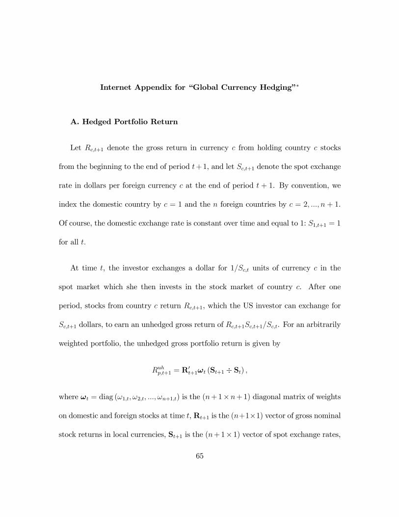
Internet Appendix for �Global Currency Hedging��

A. Hedged Portfolio Return

Let Rc;t+1 denote the gross return in currency c from holding country c stocks

from the beginning to the end of period t+1, and let Sc;t+1 denote the spot exchange

rate in dollars per foreign currency c at the end of period t + 1. By convention, we

index the domestic country by c = 1 and the n foreign countries by c = 2; :::; n + 1.

Of course, the domestic exchange rate is constant over time and equal to 1: S1;t+1 = 1

for all t:

At time t, the investor exchanges a dollar for 1=Sc;t units of currency c in the

spot market which she then invests in the stock market of country c. After one

period, stocks from country c return Rc;t+1, which the US investor can exchange for

Sc;t+1 dollars, to earn an unhedged gross return of Rc;t+1Sc;t+1=Sc;t. For an arbitrarily

weighted portfolio, the unhedged gross portfolio return is given by

Ruhp;t+1 = R0t+1!t (St+1 � St) ;

where !t = diag (!1;t; !2;t; :::; !n+1;t) is the (n+1�n+1) diagonal matrix of weights

on domestic and foreign stocks at time t, Rt+1 is the (n+1�1) vector of gross nominal

stock returns in local currencies, St+1 is the (n+1� 1) vector of spot exchange rates,

65

and � denotes the element-by-element ratio operator, so that the c-th element of

(St+1 � St) is Sc;t+1=Sc;t. The weights add up to 1 in each period t:

n+1Pc=1

!c;t = 1 8t: (A1)

We next consider the hedged portfolio. Let Fc;t denote the one-period forward

exchange rate in dollars per foreign currency c, and �c;t the dollar value of the amount

of forward exchange rate contracts for currency c the investor enters into at time t

per dollar invested in her stock portfolio.1 At the end of period t+1, the investor gets

to exchange �c;t=Sc;t units of the foreign-currency denominated return Rc;t+1!c;t=Sc;t

back into dollars at an exchange rate Fc;t. She then exchanges the rest, which amounts

to (Rc;t+1!c;t=Sc;t � �c;t=Sc;t) units of foreign currency c, at the spot exchange rate

Sc;t+1. Collecting returns for all countries leads to a hedged portfolio return Rhp;t+1 of

Rhp;t+1 = R0t+1!t (St+1 � St)��0

t (St+1 � St) +�0t (Ft � St) , (A2)

whereFt is the (n+1�1) vector of forward exchange rates, and�t = (�1;t; �2;t; :::; �n;t; �n+1;t)0.

Of course, since S1t = F1;t = 1 for all t, the choice of domestic hedge ratio �1;t is ar-

bitrary. For convenience, we set it so that all hedge ratios add up to 1:

�1;t = 1�n+1Pc=2

�c;t: (A3)

Under covered interest parity, the forward contract for currency c trades at Fc;t =

66

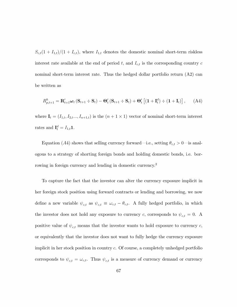
Sc;t(1 + I1;t)=(1 + Ic;t), where I1;t denotes the domestic nominal short-term riskless

interest rate available at the end of period t, and Ic;t is the corresponding country c

nominal short-term interest rate. Thus the hedged dollar portfolio return (A2) can

be written as

Rhp;t+1 = R0t+1!t (St+1 � St)��0

t (St+1 � St) +�0t

�(1+ Idt )� (1+ It)

�, (A4)

where It = (I1;t; I2;t:::; In+1;t) is the (n+ 1� 1) vector of nominal short-term interest

rates and Idt = I1;t1.

Equation (A4) shows that selling currency forward� i.e., setting �c;t > 0� is anal-

ogous to a strategy of shorting foreign bonds and holding domestic bonds, i.e. bor-

rowing in foreign currency and lending in domestic currency.2

To capture the fact that the investor can alter the currency exposure implicit in

her foreign stock position using forward contracts or lending and borrowing, we now

de�ne a new variable c;t as c;t � !c;t � �c;t. A fully hedged portfolio, in which

the investor does not hold any exposure to currency c, corresponds to c;t = 0. A

positive value of c;t means that the investor wants to hold exposure to currency c,

or equivalently that the investor does not want to fully hedge the currency exposure

implicit in her stock position in country c. Of course, a completely unhedged portfolio

corresponds to c;t = !c;t. Thus c;t is a measure of currency demand or currency

67

exposure. Accordingly we refer to c;t as currency demand or currency exposure

indistinctly.

For convenience, we now rewrite equation (A4) in terms of currency demands:

Rhp;t+1 = R0t+1!t (St+1 � St)� 10!t

�(St+1 � St)� (1+ Idt )� (1+ It)

�+0

t

�(St+1 � St)� (1+ Idt )� (1+ It)

�; (A5)

where t =� 1;t; 2;t; :::; n+1;t

�0.

Note that t = !t1��t. Given the de�nition of c;t, equations (A1) and (A3)

imply that

1;t = �n+1Pc=2

c;t: (A6)

or 0t1 = 0, so that 1;t indeed represents the domestic currency exposure. That

currency demands must add to zero is intuitive. Since the investor is fully invested in

stocks, she can achieve a long position in a particular currency c only by borrowing�

or equivalently, by shorting bonds� in her own domestic currency, and investing the

proceeds in bonds denominated in that currency. Thus the currency portfolio is a

zero investment portfolio.

B. Log Portfolio Returns Over Short Time Intervals

Assuming log-normality of the hedge returns, the derivation of the optimal

68

requires an expression for the log-return on the hedged portfolio, rhedgep;t+1 . We com-

pute this log hedged return as a discrete-time approximation to its continuous-time

counterpart. In order to do this, we need to specify, in continuous time, the return

processes for stocks Pc;t, for currencies Xc;t and for interest rates Bc;t:We assume that

they all follow a geometric brownian motions:

dPc;tPc;t

= �Pcdt+ (�Pc)t dWPct ; c = 1:::n+ 1 (B1)

dBc;tBc;t

= �Bcdt; c = 1:::n+ 1 (B2)

dXc;t

Xc;t

= �Xcdt+ (�Xc)t dWXct ; c = 1:::n+ 1; (B3)

whereW Pct ; WBc

t andWXct are di¤usion processes. dPc;t

Pc;trepresents the stock return,

dBc;tBc;t

the nominal return to holding a riskless bond from country and dXc;tXc;t

the return

to holding foreign currency c:

For notational simplicity, in what follows, we are momentarily dropping time

subscripts for the standard deviations.

Using Ito�s lemma, the log returns on each asset are given by:

d logPc;t =dPc;tPc;t

� 12�2Pcdt

d logBc;t =dBc;tBc;t

� 12�2Bcdt

d logXc;t =dXc;t

Xc;t

� 12�2Xcdt:

69

Note that, because country 1 is the domestic country, which has a �xed exchange rate

of 1, we have d logX1;t = 0: This implies �X1 = �X1 = 0:

The domestic currency return on foreign stock is then given by dPc;tXc;tPc;tXc;t

. To derive

an expression for this return, we will note that the return dynamics above, by standard

calculations, imply :

logPc;tXc;t = logPc;0Xc;0 +

��Pc + �Xc �

1

2�2Pc �

1

2�2Xc

�t

+�Pc�W Pct �W Pc

0

�+ �Xc

�WXct �WXc

0

�Di¤erentiating, and then applying Ito�s lemma, yields :

dPc;tXc;t

Pc;tXc;t

=dPc;tPc;t

+dXc;t

Xc;t

+ �Pc�Xc�Pc;Xcdt (B4)

dPc;tXc;t

Pc;tXc;t

= d logPc;t + d logXc;t +1

2Vart (pc;t + xc;t) dt, (B5)

where xc;t = d logXc;t and pc;t = dlogPc;t: Note that for c=1, the formula does yield

the simple stock return as dP1;tX1;tP1;tX1;t

= dP1;tP1;t

+ dX1;tX1;t

+ �P1�X1�P1;X1dt =dP1;tP1;t

:

A similar calculation yields the following dynamics for the return of the strategy

consisting in holding the domestic bond and shorting the foreign one :

d (B1;t=Bc;t)

B1;t=Bc;t= d logB1;t � d logBc;t (B6)

We note Vt the value of the portfolio.The log return on the portfolio, by Ito�s

70

lemma, is :

d log Vt =dVtVt� 12

�dVtVt

�2:

We can now derive each of the right-hand side terms:

dVtVt

=

n+1Xc=1

!c;t

�dPc;tXc;t

Pc;tXc;t

�+

n+1Xc=1

�c!c;td (B1;t=Bc;t)

B1;t=Bc;t�

n+1Xc=1

�c!c;tdXc;t

Xc;t

;

which follows from our convention regarding the domestic country.

Using expressions (B3) ; (B5) ; and (B6) to substitute and moving to matrix

notation, we get :

dVtVt

= 10! (pt+1 + xt+1)��0t

�xt+1 � bdt + bt

�+1

2[10!tdiag (Vart (pt+1 + xt+1))��0

tdiag (Vart xt+1)] dt ,

where pt+1 = (d logP1;t; d logP2;t:::; d logPn+1;t)0 ; xt+1 = (d logX1;t; d logX2;t:::; d logXn+1;t)

0,

bdt = (d logB1;t)1, bt = (d logB1;t; d logB2;t:::; d logBn+1;t)0 and diag (X) denotes,

for a symmetric (n� n) matrix X; the (n� 1) vector of its diagonal terms:

71

Then,

�dVtVt

�2= Vart

�10!t (pt+1 + xt+1)��0

t

�xt+1 � bdt + bt

��dt+ o (dt)

=

2666666410!tVart (pt+1 + xt+1)!t�

�210!t covt�pt+1 + xt+1;xt+1 � bdt + bt

��t

+�0!tVart�xt+1 � bdt + bt

��t

37777775 dt+ o (dt) :

So, �nally,

d log Vt = 10!t (pt+1 + xt+1)��0t

�xt+1 � bdt + bt

�(B7)

+1

2[10!tdiag (Vart (pt+1 + xt+1))��0

tdiag (Vart xt+1)] dt

�12Vart

�10!t (pt+1 + xt+1)��0

t

�xt+1 � bdt + bt

��dt+ o (dt) .

Now, we get the approximation for rhp;t+1 by computing the previous expression

for dt = 1, replacing d logXc;t = �sc;t+1; dlogPc;t = rc;t+1; and dlogBc;t = ic;t and

neglecting the higher order terms: Noting, for any variable, zt, the (n+ 1� 1) vector

(z1;t; z2;t::zn+1;t) ; this is equivalent to replacing in equation (B7) pt+1 by rt+1, xt+1

by �st+1, bdt by idt and bt by it:

rhp;t+1 ' 10!t (rt+1 +�st+1)��0t

��st+1 � idt + it

�+1

2�ht

72

where �ht+1 is equal to :

�ht = 10!tdiag (Vart (rt+1 +�st+1))��0tdiag (Vart�st+1)

�Vart�10!t (rt+1 +�st+1)��0

t

��st+1 � idt + it

��where, for any variable z, zt denotes the vector of country observations (z1;t; z2;t:::zn+1;t)

0

and small case letters denote logs in the following fashion : rc;t+1 = log (Rc;t+1) ;

st+1 = log (St+1) ; idt = log (1 + I1;t)1 and ic;t = log (1 + Ic;t) :

We can now rewrite the portfolio return as a function of t by substituting for

�t. This yields :

rhp;t+1 = 10!t�rt+1 + i

dt � it

�+0

t

��st+1 � idt + it

�+1

2�ht

= id1;t + 10!t (rt+1 � it) +0

t

��st+1 � idt + it

�+1

2�ht ;

where:

�ht = 10!t diag (Vart (rt+1 +�st+1))� (�t + !t1)0 diag (Vart (�st+1)) (B8)

�Vart�10!t

�rt+1 + i

dt � it

�+0

t

��st+1 � idt + it

��:

73

C. Equivalence Between Forward Contracts and Foreign Currency Bor-

rowing and Lending

With the same notations and assumptions as above, when the investor uses forward

contracts to hedge currency risk, the portfolio return is:

Rhp;t+1 = R0t+1!t (St+1 � St)��0

t

�(St+1 � St)� (1+ Idt )� (1+ It)

�Another natural view is one in which the investor borrows in foreign currency and

lends in domestic currency to hedge currency risk. Then, the portfolio return is:

RBLp;t+1 = R0t+1!t (St+1 � St)��0 (St+1 � St) (1 + It) +�0 �1 + Idt �

Then, with V BLt the value of the portfolio with borrowing and lending, we have in

continuous time:

dV BLt

V BLt

=n+1Xc=1

!c;t

�dPc;tXc;t

Pc;tXc;t

��

n+1Xc=1

�c;tdXc;tBc;tXc;tBc;t

+n+1Xc=1

�c;tdB1;tB1;t

=

n+1Xc=1

!c;t

�logPc;t + logXc;t +

1

2Vart (pc;t + xc;t) dt

�

�n+1Xc=1

�c;t

�log (Xc;t) + log (Bc;t) +

1

2Vart (xc;t) dt

�

+

n+1Xc=2

�c;t log (B1;t)

= 10!t (pt+1 + xt+1)��0�xt+1 + bt � bdt

�+1

210!t diagVart (pt+1 + xt+1) dt

�12�0 diagVart (xt+1) dt

74

and �dV BL

t

V BLt

�2= Vart

�!0t (pt+1 + xt+1)��0

�xt+1 + bt � bdt

��dt+ o (dt) :

So

d log V BLt =

dV BLt

V BLt

� 12

�dV BL

t

V BLt

�2= !0t (pt+1 + xt+1)��0 �xt+1 + bt � bdt �+ 12!0t diagVart (pt+1 + xt+1) dt

�12�0 diagVart (xt+1) dt

�12Vart

�!0t (pt+1 + xt+1)��0 �xt+1 + bt � bdt �� dt+ o (dt)

We now go to the limit of dt = 1 and get :

rBLp;t+1 ' 10!t (rt+1 +�st+1)��0 ��st+1 + it � idt �+ 12�ht= rhp;t+1

D. Mean-Variance Optimization

D.1. Unconstrained Hedge Ratio

In the general case, rhp;t+1� id1;t = 10!t (rt+1 � it)+0t��st+1 � idt + it

�+ 12�ht ; and

the Lagrangian is:

$�e� =

1

2(1� �)Vart

�10!t (rt+1 � it) + 0t

��st+1 � idt + it

��+�

��H � Et

�10!t (rt+1 � it) + 0t

��st+1 � idt + it

��� 12�ht

�75

Substituting for �ht using equation (B8), this expression is equivalent to :

$�e� =

1

2Vart

�10!t (rt+1 � it) + 0t

��st+1 � idt + it

��+���H � Et

�10!t (rt+1 � it)�0t

��st+1 � idt + it

�����2

�10!t diag (Vart (rt+1 +�st+1))� (!t1�t)0 diag (Vart (�st+1))

�$�e� =

1

2Vart

�0t��st+1 � idt + it

��� �Et

�0t��st+1 � idt + it

����20t diag (Vart (�st+1))

+ covt�10!t (rt+1 � it) ;0t

��st+1 � idt + it

��+1

2Vart (1

0!t (rt+1 � it))� �Et (10!t (rt+1 � it))

+�

210!t [diag (Vart (�st+1))� diag (Vart (rt+1 +�st+1))]

+��H

$�e� =

1

20tVart

��st+1 � idt + it

�t � �0t

2664 Et��st+1 � idt + it

�+12diag (Vart (�st+1))

3775+covt

�10!t (rt+1 � it) ;

��st+1 � idt + it

��t

+K (�)

where

K (�) = ��H +1

2Vart (1

0!t (rt+1 � it))� �Et (10!t (rt+1 � it))

+�

210!t [diag (Vart (�st+1))� diag (Vart (rt+1 +�st+1))]

76

K (�) is independent of et.Now, we need to solve only for et as 1; the demand for domestic currency, is

given once the other currency demands are determined. We rewrite the Lagrangian

in terms of et:$�e� =

1

2e0tVart �f�st+1 �eidt +eit� et � �e0t

2664 Et

�f�st+1 �eidt +eit�+12diag

�Vart

�f�st+1��3775

+covt

�10!t (rt+1 � it) ;

�f�st+1 �eidt +eit�� et+K (�)

The F.O.C. gives the following expression for the optimal et :0 = covt

�10!t (rt+1 � it) ;

�f�st+1 �eidt +eit��+Vart

�f�st+1 �eidt +eit� e�t � �

�Et

�f�st+1 �eidt +eit�+ 12 diag �Vart �f�st+1���

Finally, the optimal vector of currency demands is :

e�t (�) = �Var�1t

�f�st+1 �eidt +eit��Et �f�st+1 �eidt +eit�+ 12diag �Vart f�st+1��

�Var�1t�f�st+1 �eidt +eit� hcovt �10!t (rt+1 � it) ;�f�st+1 �eidt +eit��i

77

D.2. Constrained Hedge Ratio

In the case where et = te1 (where e1 denotes an n� 1 vector of ones), we note �tthe optimal scalar constrained hedge ratio and we have :

$ ( t) =1

2 2te10Vart �f�st+1 �eidt +eit�e1� � te10

2664 Et

�f�st+1 �eidt +eit�+12diag

�Vart

�f�st+1��3775

+ t covt

�10!t (rt+1 � it) ;

�f�st+1 �eidt +eit��e1+K (�)

and

�t =�e10 hEt �f�st+1 �eidt +eit�+ 1

2diag

�Vart

�f�st+1��ie10Vart �f�st+1 �eidt +eit�e1�covt

�10!t (rt+1 � it) ;

�f�st+1 �eidt +eit��e1e10Vart �f�st+1 �eidt +eit�e1In this case, �t can equivalently be written in terms of the full matrices :

�t =�10

�Et��st+1 � idt + it

�+ 1

2diag (Vart (�st+1))

�10Vart

��st+1 � idt + it

�1

�10 covt

�!t (rt+1 � it) ;

��st+1 � idt + it

��1

10Vart��st+1 � idt + it

�1

78

This case corresponds to a domestic investor hedging the same ratio of his foreign

stock holdings for all foreign currencies.

E. Invariance of Optimal Currency Demand With Respect to Base

Country

In the system of n2 bilateral exchange rates, there are really only n free parameters

as all exchange rates can be backed out of the n bilateral rates for one base domestic

country. We use this fact to show that, for a portfolio of stocks from the n + 1

countries in our model, the optimal hedge ratios on stocks from country c; j�c is the

same for any base country j. Let us now use the subscript j to index the domestic

country.

We assume for this derivation that weights on international stocks are the same

for investors from all countries so that !jt = !t: In terms of our empirical tests, this

result will hence apply to the cases of an equally weighted or a value weighted world

portfolios, in which weights do not vary with the base country. They do not hold for

a home biased porftolio, in which weights by de�nition vary with base country.

Let us think of country 1 as our base country, and write the optimal vector of

foreign currency demand assuming that �j = 0 for all values of j: We have :

79

e1�RM = �Vart

�f�s1t+1 �ei1;dt +ei1t��1 hcovt �10!t (rt+1 � it) ; f�s1t+1 �ei1;dt +ei1t�i= �Vart

�ex1t+1��1 �covt �yWt+1; ex1t+1��where x1t+1 = �s

1t+1 � i1;dt + i1t and y

Wt+1 = 1

0!t (rt+1 � it) :

Now, let us consider exchange rates from the perspective of country 2. By de�ni-

tion of the exchange rate between countries 1 and 2, it follows that s2t+1;1 = �s1t+1;2:

Also, by de�nition of the exchange rates, S2t+1;3 units of currency 2 can be ex-

changed into one unit of currency 3. And one unit of currency 3 is equivalent to

S1t+1;3 units of currency 1, which is equivalent to S1t+1;3=S

1t+1;2 units of currency 2.

So, the absence of arbitrage implies the equality: S2t+1;3 = S1t+1;3=S1t+1;2: In logs,

s2t+1;3 = s1t+1;3� s1t+1;2: More generally, the following equality can be derived from the

absence of arbitrage:

s2t+1;c = s1t+1;c � s1t+1;2 c = 3:::n+ 1

In matrix notation, this amounts to a linear relationship between f�s2t+1 and f�s1t+1:f�s2t+1 = A2 � f�s1t+1

80

where A2 =

0BBBBBBBBBBBBBB@

-1 0 .. .. 0

-1 1 0 .. ..

-1 0 1 0 ..

-1 0 0 .. 0

-1 0 .. 0 1

1CCCCCCCCCCCCCCA:

Given our notations :

ei1;dt �ei1t = (it;2 � it;1; it;3 � it;1; ::it;n+1 � it;1)0

and

ei2;dt �ei2t = (it;1 � it;2; it;3 � it;2; ::; it;n+1 � it;2)0 :

It follows that: ei2;dt �ei2t = A�ei1;dt �ei1t� :

Similarly, we have the following linear relationship between ex2t+1 and ex1t+1:ex2t+1 = Aex1t+1 , (E1)

Let us substitute equation (E1), the formula for ex2t+1; into equation (??), the formulafor the optimal hedge ratio. We use the properties of matrix second moments that

81

Var (AX) = AVar (X)A0, cov(AX; Y ) = Acov (X; Y ) ; and the property of inverse

matrices that (AB)�1 = B�1A�1: Also, we note that A2 = (A2)�1 and (A02)

�1 = A02.

Substitution yields:

e2�RM = �Vart

�ex2t+1��1 �covt �yWt+1; ex2t+1��= � (A02)

�1Vart

�ex1t+1��1 (A2)�1 �A2 covt �ex1t+1;yWt+1��e2�RM

��2�= � (A02)

�1Vart

�ex1t+1��1 covt �ex1t+1;yWt+1�e2� = A02

e1�

We write out the vector e2�RM :

e2�RM =

��n+1Pc=2

1�c ;1�3 ;

1�4 ; ::;

1�n+1

�

Given the property thatn+1Pc=1

j�c = 1 for j = 1::n+1, 1�1 = �

n+1Pc=2

1�c so that e2�RM =�

1�1 ;1�3 ;

1�4 ; ::;

1�n+1

�: Applying this same property twice, 2�2 = �

n+1Pc 6=22�c =

�n+1Pc 6=21�c = 1�2 , so that:

2�RM =

�1�1 ;

1�2 ;

1�3 ;

1�4 ; ::;

1�n+1

�= 1�RM : Finally, the

vector of optimal currency positions is the same for investors based in country 2 as

that of country 1 investors.

82

Similar results hold for j = 3:::n + 1; where A3 =

0BBBBBBBBBBBBBB@

1 -1 .. .. 0

0 -1 0 .. ..

0 -1 1 0 ..

0 .. 0 .. 0

0 -1 .. 0 1

1CCCCCCCCCCCCCCA, A4 =

0BBBBBBBBBBBBBB@

1 0 -1 .. 0

0 1 .. .. ..

0 0 -1 0 ..

0 .. .. 1 0

0 -1 -1 0 1

1CCCCCCCCCCCCCCA, etc...

This analysis justi�es dropping the base-country subscript j and interpreting the

(n+ 1� 1) vector� =

��n+1Pc=2

1�c ;1�2 ;

1�3 ; ::;

1�n+1

�0as a common vector of foreign

currency demands that is independent of the country of origin.

A situation in which investors from all countries are hedged perfectly corresponds

to � = (0; 0; ::; 0)0 :

A situation in which investors from country 1 are not hedged at all corresponds

to � =��1; !12; !13::; !1n+1

�0: That is, investors from country i undo the hedge of the

fully hedged portfolio by taking long positions in each foreign currency proportional

83

to the weight of each foreign country in their stock portfolio. (The perfectly hedged

portfolio obtains by shorting each foreign currency by that same amount.) They need

to borrow one unit of domestic currency to �nance that.

Finally, note that this proof relies on the fact that all relevant exchange rates for

an investor in a given base country are linear combinations of the relevant exchange

rates for each other base country. In other words, the assumption is that all investors

optimize over the same set of currencies.

F. Computation of Sharpe Ratios

Table A14 reports in-sample Sharpe Ratios generated by the set of currency hedg-

ing strategies for global portfolios of stocks and bonds considered in the paper. The

denominator of the Sharpe ratio is given by the standard deviations of log portfolio

returns reported in Table VII of the main text.

The numerator of the Sharpe ratio is given by the log of the mean gross return

on each of the portfolios. We compute a time series of gross returns for each strategy

using equation (A5), where t is resplaced by the vector of �xed or time-varying

currency demands that corresponds to each currency hedging strategy� for example,

t is a vector of zeroes for the �Full Hedge�strategy. Next we average the time series

of gross returns, and take the natural log of the arithmetic mean.

84

Thus our Sharpe ratio is computed as

log�E�Rhp;t+1

��qVar

�rhp;t+1

� ;which at high frequency observation of returns or under lognormality is equivalent to

E�rhp;t+1

�+ 1

2Var

�rhp;t+1

�qVar

�rhp;t+1

� :

85

Internet Appendix Endnotes

*. Citation format: John Y. Campbell, Karine Serfaty-de Medeiros, and Luis M.

Viceira, Global currency hedging, Journal of Finance [-volume-], [-pages-], Internet

Appendix http://www.afajof.org/supplements.asp.

1. That is, at the end of month t, the investor can enter into a forward contract

to sell one unit of currency c at the end of month t + 1 for a forward price of Fc;t

dollars.

2. Note, however, that the two strategies are not completely equivalent except in

the continuous time limit. We show in Appendix B that, in continuous time, the two

strategies are exactly equivalent.

86

Euroland Australia Canada Japan Switzerland UK USBase country: EurolandEuroland .Australia . 1.00Canada . 0.70 1.00Japan . 0.35 0.35 1.00Switzerland . -0.09 -0.11 0.20 1.00UK . 0.31 0.34 0.24 -0.02 1.00US . 0.63 0.87 0.40 -0.07 0.38 1.00

Base country: AustraliaEuroland 1.00Australia . .Canada 0.53 . 1.00Japan 0.67 . 0.46 1.00Switzerland 0.92 . 0.47 0.69 1.00UK 0.78 . 0.51 0.59 0.72 1.00US 0.59 . 0.85 0.55 0.54 0.58 1.00

Base country: CanadaEuroland 1.00Australia 0.23 1.00Canada . . .Japan 0.59 0.25 . 1.00Switzerland 0.91 0.20 . 0.62 1.00UK 0.71 0.24 . 0.50 0.65 1.00US 0.32 0.11 . 0.35 0.31 0.34 1.00

Base Country: JapanEuroland 1.00Australia 0.46 1.00Canada 0.55 0.74 1.00Japan . . . .Switzerland 0.87 0.33 0.39 . 1.00UK 0.72 0.49 0.56 . 0.60 1.00US 0.55 0.67 0.90 . 0.41 0.58 1.00

Base Country: SwitzerlandEuroland 1.00Australia 0.47 1.00Canada 0.52 0.77 1.00Japan 0.31 0.46 0.47 1.00Switzerland . . . . .UK 0.56 0.49 0.53 0.37 . 1.00US 0.51 0.71 0.91 0.51 . 0.55 1.00

Base Country: UKEuroland 1.00Australia 0.35 1.00Canada 0.42 0.71 1.00Japan 0.50 0.42 0.44 1.00Switzerland 0.84 0.25 0.30 0.52 1.00UK . . . . . .US 0.42 0.64 0.88 0.48 0.32 . 1.00

Base Country: USEuroland 1.00Australia 0.26 1.00Canada 0.18 0.43 1.00Japan 0.55 0.25 0.10 1.00Switzerland 0.90 0.21 0.12 0.58 1.00UK 0.69 0.25 0.14 0.44 0.61 1.00US . . . . . . .

Note. This table presents cross-country correlations of foreign currency log excess returns s c,t +i c,t -i d,t , where d indexes the basecountry. Correlations are presented separately for investors from each base country. They are computed using monthly returns.

Table A1Currency return correlations

Euroland Australia Canada Japan Switzerland UK USEuroland -0.37*** -0.45*** -0.25*** 0.28* -0.30*** -0.33***

(0.09) (0.10) (0.07) (0.15) (0.09) (0.11)Australia 0.37*** 0.02 0.14* 0.33*** 0.21** 0.16**

(0.09) (0.08) (0.07) (0.07) (0.09) (0.08)Canada 0.45*** -0.02 0.15* 0.38*** 0.25** 0.55***

(0.10) (0.08) (0.09) (0.09) (0.11) (0.16)Japan 0.25*** -0.14* -0.15* 0.32*** 0.05 -0.06

(0.07) (0.07) (0.09) (0.08) (0.06) (0.09)Switzerland -0.28* -0.33*** -0.38*** -0.32*** -0.29*** -0.30***

(0.15) (0.07) (0.09) (0.08) (0.07) (0.09)UK 0.30*** -0.21** -0.25** -0.05 0.29*** -0.13

(0.09) (0.09) (0.11) (0.06) (0.07) (0.11)US 0.33*** -0.16** -0.55*** 0.06 0.30*** 0.13

(0.11) (0.08) (0.16) (0.09) (0.09) (0.11)

Cells of Panel A are obtained by regressing the excess return to the global equity portfolio onto the excess return of thecolumn country currency to an investor based in the row country. All regressions include an intercept.Reported currency positions are the amount of dollars invested in foreign currency per dollar in the portfolio.We run monthly regressions on overlapping quarterly returns. Standard errors are corrected for auto-correlation due tooverlapping intervals using the Newey-West procedure.

Table A2

Base countryCurrency

Optimal currency exposure for an equally-weighted global equity portfolio: single-currency case

Note. This table considers an investor holding a portfolio composed of stocks from all countries, with equal weights, whochooses a position in one foreign currency at a time to minimize the variance of his portfolio. Rows indicate the basecountry of the investor, columns the currencies used to manage risk.

Euroland Australia Canada Japan Switzerland UK USPanel A : 7 country optimization1 month 0.17 -0.16 -0.61* -0.11 0.23 -0.11 0.60*

(0.15) (0.11) (0.14) (0.07) (0.12) (0.08) (0.15)2 months 0.29 -0.13 -0.63* -0.19* 0.26 -0.11 0.51*

(0.15) (0.09) (0.15) (0.07) (0.13) (0.09) (0.15)3 months 0.32 -0.11 -0.61* -0.17 0.27 -0.10 0.40*

(0.17) (0.09) (0.16) (0.09) (0.15) (0.11) (0.18)6 months 0.20 -0.05 -0.38 -0.25* 0.35 -0.06 0.19

(0.26) (0.14) (0.25) (0.12) (0.20) (0.16) (0.28)12 months -0.20 0.21 -0.22 -0.41* 0.67* -0.20 0.15

(0.40) (0.20) (0.36) (0.17) (0.30) (0.21) (0.37)

Panel B : 5 country optimization1 month 0.37* -0.29* -0.08 -0.10 0.11

(0.11) (0.11) (0.07) (0.08) (0.08)2 months 0.50* -0.27* -0.15* -0.09 0.01

(0.11) (0.09) (0.07) (0.09) (0.11)3 months 0.56* -0.27* -0.14 -0.09 -0.06

(0.11) (0.10) (0.08) (0.11) (0.14)6 months 0.53* -0.21 -0.21* -0.02 -0.09

(0.14) (0.13) (0.10) (0.15) (0.18)12 months 0.44* 0.05 -0.34* -0.16 0.01

(0.19) (0.17) (0.15) (0.19) (0.22)

Rows indicate the time-horizon T of the investor, columns the currencies used to manage risk.

Rows are obtained by regressing the excess return on the global equity portfolio onto the vector of all foreign currencyexcess returns. All regressions include an intercept. All returns considered are at the row time-horizon.

Reported currency positions are the amount of dollars invested in foreign currency per dollar in the portfolio.

We run monthly regressions on overlapping T -months returns, T varying from 1 month to 12 months. Standard errorsare corrected for auto-correlation due to overlapping intervals using the Newey-West procedure.

Note. This table considers an investor holding a portfolio composed of stocks from all countries, with equal weights,who chooses a vector of positions in all available foreign currencies to minimize the variance of his portfolio. In thiscase, the optimal currency positions do not depend on the investor's base country.

Table A3

Time horizonCurrency

Optimal currency exposure for an equally-weighted global equity portfolio: multiple-currency case

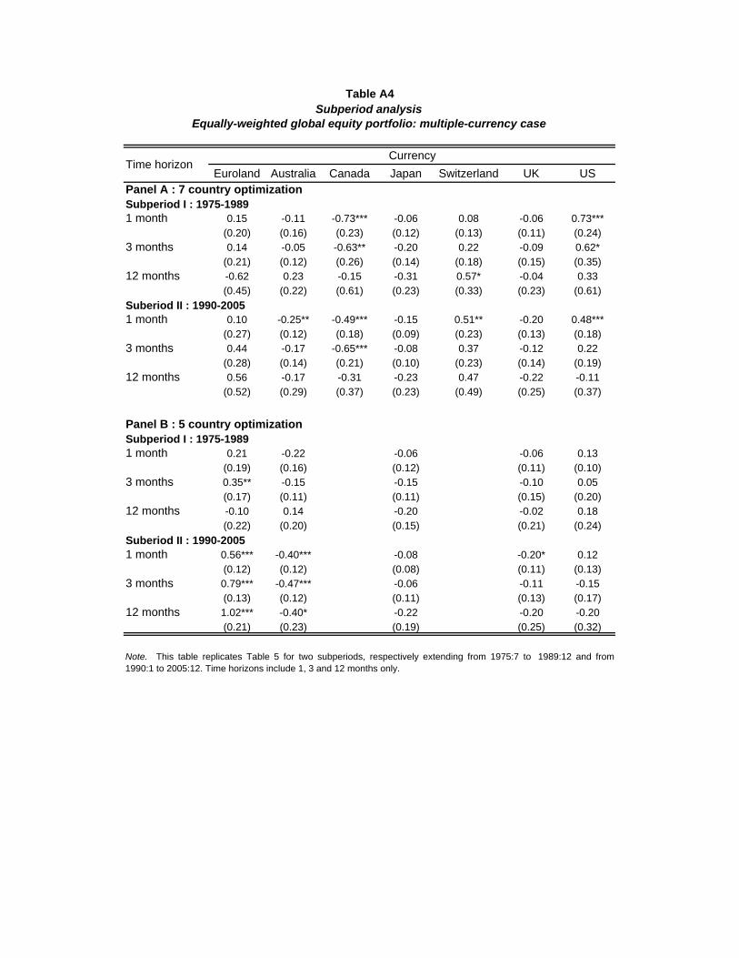
Euroland Australia Canada Japan Switzerland UK USPanel A : 7 country optimizationSubperiod I : 1975-19891 month 0.15 -0.11 -0.73*** -0.06 0.08 -0.06 0.73***

(0.20) (0.16) (0.23) (0.12) (0.13) (0.11) (0.24)3 months 0.14 -0.05 -0.63** -0.20 0.22 -0.09 0.62*

(0.21) (0.12) (0.26) (0.14) (0.18) (0.15) (0.35)12 months -0.62 0.23 -0.15 -0.31 0.57* -0.04 0.33

(0.45) (0.22) (0.61) (0.23) (0.33) (0.23) (0.61)Suberiod II : 1990-20051 month 0.10 -0.25** -0.49*** -0.15 0.51** -0.20 0.48***

(0.27) (0.12) (0.18) (0.09) (0.23) (0.13) (0.18)3 months 0.44 -0.17 -0.65*** -0.08 0.37 -0.12 0.22

(0.28) (0.14) (0.21) (0.10) (0.23) (0.14) (0.19)12 months 0.56 -0.17 -0.31 -0.23 0.47 -0.22 -0.11

(0.52) (0.29) (0.37) (0.23) (0.49) (0.25) (0.37)

Panel B : 5 country optimizationSubperiod I : 1975-19891 month 0.21 -0.22 -0.06 -0.06 0.13

(0.19) (0.16) (0.12) (0.11) (0.10)3 months 0.35** -0.15 -0.15 -0.10 0.05

(0.17) (0.11) (0.11) (0.15) (0.20)12 months -0.10 0.14 -0.20 -0.02 0.18

(0.22) (0.20) (0.15) (0.21) (0.24)Suberiod II : 1990-20051 month 0.56*** -0.40*** -0.08 -0.20* 0.12

(0.12) (0.12) (0.08) (0.11) (0.13)3 months 0.79*** -0.47*** -0.06 -0.11 -0.15

(0.13) (0.12) (0.11) (0.13) (0.17)12 months 1.02*** -0.40* -0.22 -0.20 -0.20

(0.21) (0.23) (0.19) (0.25) (0.32)

Time horizonCurrency

Note. This table replicates Table 5 for two subperiods, respectively extending from 1975:7 to 1989:12 and from1990:1 to 2005:12. Time horizons include 1, 3 and 12 months only.

Subperiod analysisTable A4

Equally-weighted global equity portfolio: multiple-currency case

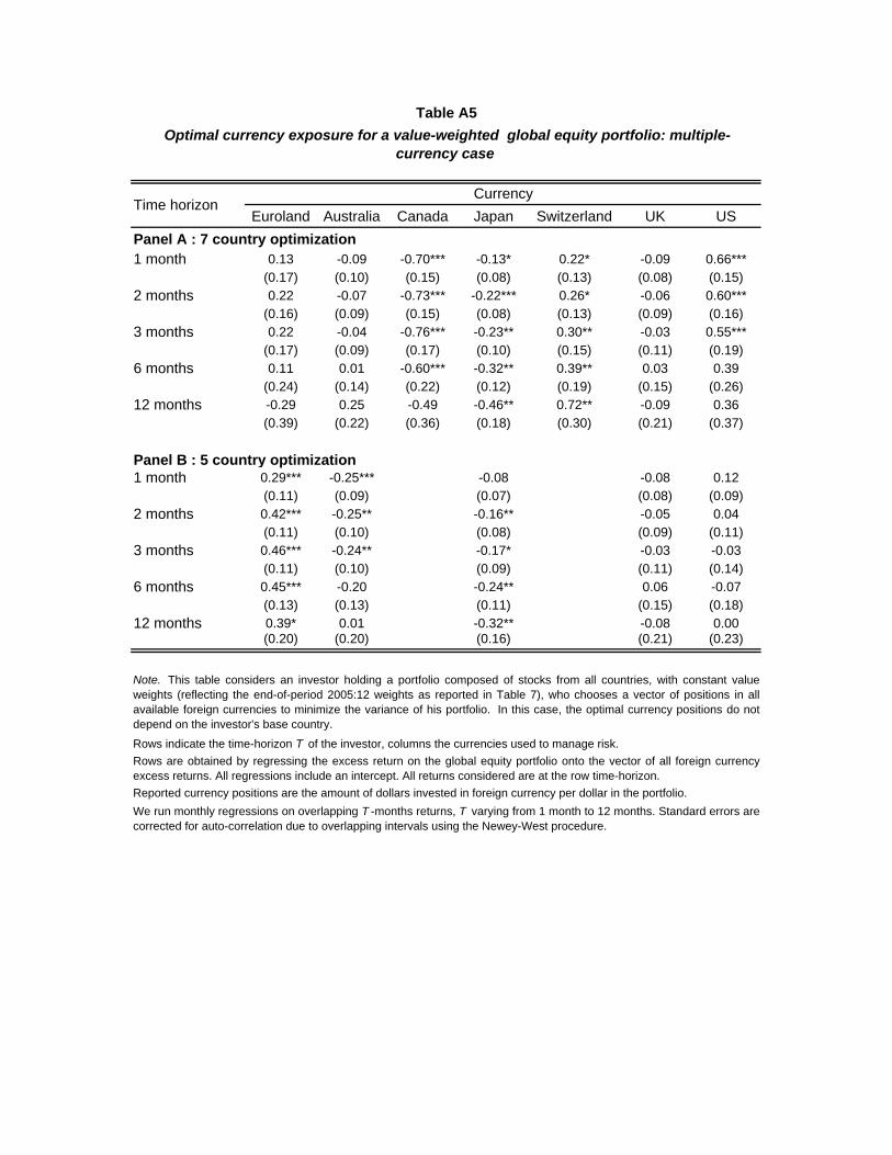
Euroland Australia Canada Japan Switzerland UK USPanel A : 7 country optimization1 month 0.13 -0.09 -0.70*** -0.13* 0.22* -0.09 0.66***

(0.17) (0.10) (0.15) (0.08) (0.13) (0.08) (0.15)2 months 0.22 -0.07 -0.73*** -0.22*** 0.26* -0.06 0.60***

(0.16) (0.09) (0.15) (0.08) (0.13) (0.09) (0.16)3 months 0.22 -0.04 -0.76*** -0.23** 0.30** -0.03 0.55***

(0.17) (0.09) (0.17) (0.10) (0.15) (0.11) (0.19)6 months 0.11 0.01 -0.60*** -0.32** 0.39** 0.03 0.39

(0.24) (0.14) (0.22) (0.12) (0.19) (0.15) (0.26)12 months -0.29 0.25 -0.49 -0.46** 0.72** -0.09 0.36

(0.39) (0.22) (0.36) (0.18) (0.30) (0.21) (0.37)

Panel B : 5 country optimization1 month 0.29*** -0.25*** -0.08 -0.08 0.12

(0.11) (0.09) (0.07) (0.08) (0.09)2 months 0.42*** -0.25** -0.16** -0.05 0.04

(0.11) (0.10) (0.08) (0.09) (0.11)3 months 0.46*** -0.24** -0.17* -0.03 -0.03

(0.11) (0.10) (0.09) (0.11) (0.14)6 months 0.45*** -0.20 -0.24** 0.06 -0.07

(0.13) (0.13) (0.11) (0.15) (0.18)12 months 0.39* 0.01 -0.32** -0.08 0.00

(0.20) (0.20) (0.16) (0.21) (0.23)

Reported currency positions are the amount of dollars invested in foreign currency per dollar in the portfolio.We run monthly regressions on overlapping T -months returns, T varying from 1 month to 12 months. Standard errors arecorrected for auto-correlation due to overlapping intervals using the Newey-West procedure.

Note. This table considers an investor holding a portfolio composed of stocks from all countries, with constant valueweights (reflecting the end-of-period 2005:12 weights as reported in Table 7), who chooses a vector of positions in allavailable foreign currencies to minimize the variance of his portfolio. In this case, the optimal currency positions do notdepend on the investor's base country.

Time horizonCurrency

Table A5 Optimal currency exposure for a value-weighted global equity portfolio: multiple-

currency case

Rows indicate the time-horizon T of the investor, columns the currencies used to manage risk.Rows are obtained by regressing the excess return on the global equity portfolio onto the vector of all foreign currencyexcess returns. All regressions include an intercept. All returns considered are at the row time-horizon.

Euroland Australia Canada Japan Switzerland UK USPANEL A : Single currencyEuroland -0.40*** -0.52*** -0.31*** 0.34* -0.32*** -0.45***

(0.10) (0.12) (0.08) (0.18) (0.11) (0.13)Australia 0.37*** 0.09 0.16* 0.31*** 0.17 0.25**

(0.10) (0.11) (0.09) (0.09) (0.12) (0.10)Canada 0.42*** -0.01 0.12 0.35*** 0.17 0.88***

(0.10) (0.10) (0.09) (0.09) (0.11) (0.19)Japan 0.31*** -0.09 -0.08 0.35*** 0.15* 0.02

(0.10) (0.09) (0.10) (0.10) (0.08) (0.11)Switzerland -0.45*** -0.35*** -0.42*** -0.29*** -0.29*** -0.38***

(0.15) (0.08) (0.09) (0.09) (0.08) (0.10)UK 0.25** -0.24** -0.30*** -0.10 0.25*** -0.21*

(0.11) (0.10) (0.12) (0.07) (0.09) (0.12)US 0.23** -0.14* -0.71*** -0.01 0.22** 0.11

(0.11) (0.08) (0.16) (0.09) (0.09) (0.11)

Panel B : Multiple currencies at onceEuroland 0.36 -0.08 -0.50** -0.20* 0.33* -0.08 0.17

(0.23) (0.11) (0.21) (0.11) (0.18) (0.13) (0.22)Australia 0.47** -0.16 -0.68*** -0.14 0.15 -0.24* 0.60***

(0.20) (0.12) (0.17) (0.11) (0.19) (0.15) (0.22)Canada 0.30 -0.05 -0.94*** -0.22** 0.31 -0.23* 0.83***

(0.20) (0.10) (0.21) (0.10) (0.20) (0.13) (0.21)Japan 0.34* -0.14 -0.63*** -0.25** 0.20 0.01 0.48**

(0.17) (0.13) (0.21) (0.12) (0.16) (0.12) (0.21)Switzerland 0.14 -0.12 -0.35* -0.07 0.37** -0.02 0.04

(0.21) (0.09) (0.19) (0.11) (0.17) (0.13) (0.21)UK 0.30 -0.11 -0.56*** -0.20** 0.28 -0.02 0.30

(0.21) (0.10) (0.19) (0.09) (0.18) (0.13) (0.20)US 0.15 0.00 -0.83*** -0.22** 0.30* -0.03 0.62***

(0.18) (0.09) (0.17) (0.09) (0.15) (0.11) (0.19)

Reported currency positions are the amount of dollars invested in foreign currency per dollar in the portfolio.We run monthly regressions on overlapping quarterly returns. Standard errors are corrected for auto-correlation dueto overlapping intervals using the Newey-West procedure.

Base countryCurrency

Optimal currency exposure for a home-biased global equity portfolio: single and multiple currency cases

Table A6

Note. This table considers an investor holding a home-biased portfolio of global equity. The portfolio is constructedby assigning a 75% weight to the home country of the investor, and distributing the remaining 25% over the four othercountries according to their value weights. The investor chooses a foreign currency position to minimize the varianceof his portfolio. Panel A allows the investor to use only one foreign currency. Panel B allows her to choose a vector ofpositions in all available foreign currencies. Rows indicate the base country of the investor, columns the currenciesused to manage risk.

Cells of Panel A are obtained by regressing the excess return on the row country home biased global equity portfolioonto the excess return on the column country currency. Rows of Panel B (excluding diagonal terms) are obtained byregressing the excess return on the row country portfolio on the vector of all foreign currency excess returns. Allregressions include an intercept. Diagonal terms in Panel B are obtained by computing the opposite of the sum ofother terms and the corresponding standard deviation.

Euroland Australia Canada Japan Switzerland UK USPanel A : Single currencyEuroland 0.04 0.05 -0.03 -0.02 0.09** 0.06*

(0.03) (0.03) (0.04) (0.06) (0.04) (0.04)Australia -0.02 0.04 0.00 -0.01 0.02 0.06

(0.05) (0.07) (0.05) (0.05) (0.04) (0.05)Canada -0.07 0.12** -0.07 -0.08* -0.07 0.24***

(0.05) (0.05) (0.05) (0.04) (0.06) (0.08)Japan 0.05 0.09** 0.14*** 0.01 0.10** 0.16***

(0.05) (0.04) (0.05) (0.05) (0.05) (0.05)Switzerland 0.08 0.02 0.05 -0.02 0.09** 0.05

(0.07) (0.02) (0.03) (0.04) (0.04) (0.03)UK 0.22*** 0.07** 0.11** 0.02 0.13*** 0.12***

(0.05) (0.04) (0.05) (0.04) (0.05) (0.04)US -0.21*** 0.03 -0.21** -0.15*** -0.18*** -0.09*

(0.05) (0.05) (0.09) (0.05) (0.04) (0.05)

Panel B : Multiple currenciesEuroland -0.10 0.01 -0.01 -0.07* 0.03 0.08* 0.07

(0.08) (0.03) (0.07) (0.04) (0.07) (0.05) (0.06)Australia -0.13 -0.02 -0.07 0.00 0.03 0.06 0.14

(0.15) (0.08) (0.13) (0.06) (0.12) (0.07) (0.10)Canada 0.03 0.18*** -0.35*** -0.08 -0.08 -0.07 0.36***

(0.12) (0.05) (0.11) (0.06) (0.11) (0.08) (0.08)Japan -0.05 -0.02 0.00 -0.12* -0.07 0.07 0.18*

(0.10) (0.05) (0.10) (0.06) (0.08) (0.05) (0.09)Switzerland -0.03 -0.03 0.05 -0.06 -0.04 0.10** 0.01

(0.08) (0.04) (0.08) (0.05) (0.08) (0.05) (0.07)UK 0.28** 0.01 -0.05 -0.10 -0.04 -0.23*** 0.13

(0.13) (0.06) (0.14) (0.06) (0.11) (0.06) (0.10)US -0.22* 0.19*** -0.30** -0.10 -0.02 0.09 0.36***

(0.11) (0.06) (0.12) (0.06) (0.09) (0.07) (0.09)

Optimal currency exposure for single-country bond portfolios: single and multiple currency cases

Table A7

Note. This table considers an investor holding a portfolio composed of long-term bonds from his own country, whochooses a foreign currency position to minimize the variance of his portfolio. Panel A allows the investor to use onlyone foreign currency. Panel B allows her to choose a vector of positions in all available foreign currencies. Rowsindicate the bond being held (as well as the base country), columns the currencies used to manage risk.

Cells of Panel A are obtained by regressing the hedged excess return to the row country bond onto the excess returnon the column country currency. Rows of Panel B (excluding diagonal terms) are obtained by regressing the excessreturn to the row country stock bond onto the vector of all foreign currency excess returns. All regressions include anintercept. Diagonal terms in Panel B are obtained by computing the opposite of the sum of other terms in the same rowand the corresponding standard deviation.Reported currency positions are the amount of dollars invested in foreign currency per dollar in the portfolio.We run monthly regressions on overlapping quarterly returns. Standard errors are corrected for auto-correlation due tooverlapping intervals using the Newey-West procedure.

Bond marketCurrency

Euroland Australia Canada Japan Switzerland UK USPanel A : 7 country optimization1 month 0.02 0.00 -0.12* -0.06* -0.04 -0.01 0.22*

(0.05) (0.02) (0.05) (0.03) (0.04) (0.03) (0.05)2 months -0.01 0.03 -0.14* -0.08* -0.03 0.00 0.23*

(0.07) (0.03) (0.06) (0.03) (0.05) (0.04) (0.05)3 months -0.03 0.04 -0.10 -0.07 -0.03 0.01 0.18*

(0.07) (0.04) (0.08) (0.04) (0.07) (0.05) (0.06)6 months -0.08 0.13* -0.05 -0.10 0.00 0.06 0.05

(0.11) (0.05) (0.10) (0.06) (0.10) (0.07) (0.08)12 months -0.26 0.17 0.03 -0.11 0.11 0.14 -0.08

(0.17) (0.09) (0.16) (0.08) (0.13) (0.11) (0.11)

Panel B : 5 country optimization1 month -0.02 -0.03 -0.07* -0.01 0.13*

(0.03) (0.02) (0.03) (0.03) (0.03)2 months -0.04 -0.01 -0.09* -0.01 0.15*

(0.04) (0.03) (0.03) (0.03) (0.04)3 months -0.06 0.01 -0.08 0.01 0.11*

(0.05) (0.03) (0.04) (0.05) (0.04)6 months -0.08 0.11* -0.10 0.06 0.01

(0.08) (0.04) (0.06) (0.07) (0.06)12 months -0.14 0.18* -0.10 0.12 -0.06

(0.12) (0.06) (0.07) (0.11) (0.07)

We run monthly regressions on overlapping T -months returns, T varying from 1 month to 12 months. Standard errorsare corrected for auto-correlation due to overlapping intervals using the Newey-West procedure.

Rows are obtained by regressing the excess return on the global bond portfolio onto the vector of all foreign currencyexcess returns. All regressions include an intercept. All returns considered are at the row time-horizon.

Reported currency positions are the amount of dollars invested in foreign currency per dollar in the portfolio.

Rows indicate the time-horizon T of the investor, columns the currencies used to manage risk.

Note. This table considers an investor holding a portfolio composed of bonds from all countries, with equal weights,who chooses a vector of positions in all available foreign currencies to minimize the variance of his portfolio. In thiscase, the optimal currency positions do not depend on the investor's base country.

Table A8 Optimal currency exposure for an equally-weighted global bond portfolio: multiple-

currency case

Time horizonCurrency

Euroland Australia Canada Japan Switzerland UK USPanel A : 7 country optimizationSubperiod I: 1975-19891 month 0.08 0.01 -0.24** -0.11*** -0.06 0.00 0.33***

(0.07) (0.04) (0.10) (0.04) (0.05) (0.03) (0.09)3 months -0.02 0.04 -0.30** -0.16*** -0.01 0.02 0.43***

(0.10) (0.05) (0.14) (0.06) (0.08) (0.06) (0.12)12 months -0.29* 0.24** -0.14 -0.25*** 0.12 0.20** 0.13

(0.16) (0.11) (0.19) (0.08) (0.10) (0.09) (0.14)Subperiod 2: 1990-20051 month -0.07 0.00 -0.05 -0.04 0.04 0.00 0.12**

(0.09) (0.03) (0.06) (0.03) (0.07) (0.04) (0.06)

3 months -0.17 0.13** -0.08 -0.01 0.06 0.04 0.04(0.12) (0.06) (0.11) (0.05) (0.11) (0.06) (0.06)

12 months -0.42** 0.24** -0.14 0.04 0.25* 0.12 -0.10(0.21) (0.12) (0.22) (0.09) (0.15) (0.11) (0.10)

Panel B : 5 country optimizationSubperiod I: 1975-19891 month 0.02 -0.04 -0.11** -0.01 0.15***

(0.06) (0.03) (0.04) (0.03) (0.04)3 months -0.03 -0.04 -0.14** 0.01 0.20***

(0.08) (0.04) (0.07) (0.05) (0.06)12 months -0.18 0.16* -0.21*** 0.20** 0.03

(0.12) (0.09) (0.07) (0.09) (0.11)Subperiod 2: 1990-20051 month -0.05 -0.01 -0.04 0.00 0.10**

(0.04) (0.03) (0.03) (0.04) (0.04)3 months -0.13** 0.12*** 0.00 0.03 -0.02

(0.06) (0.04) (0.05) (0.06) (0.05)12 months -0.16 0.20*** 0.04 0.08 -0.16*

(0.13) (0.05) (0.08) (0.11) (0.10)

Note. This table considers an investor holding a portfolio composed of bonds from all countries, with equal weights,who chooses a vector of positions in all available foreign currencies to minimize the variance of his portfolio. In thiscase, the optimal currency positions do not depend on the investor's base country.

Table A9- Subperiod analysis

Time horizonCurrency

Optimal currency exposure for an equally-weighted global bond portfolio: multiple-currency case

Rows indicate the time-horizon T of the investor, columns the currencies used to manage risk.

We run monthly regressions on overlapping T -months returns, T varying from 1 month to 12 months. Standard errorsare corrected for auto-correlation due to overlapping intervals using the Newey-West procedure.

Reported currency positions are the amount of dollars invested in foreign currency per dollar in the portfolio.

Rows are obtained by regressing the excess return on the global equity portfolio onto the vector of all foreign currencyexcess returns. All regressions include an intercept. All returns considered are at the row time-horizon.

Slope P-Value Slope P-Value Slope P-Value Slope P-ValueEuroland -0.10 1.00 -7.57 0.11 0.10 0.99 1.92 0.00

(0.94) (7.55) (0.34) (3.62)Australia -0.08 1.00 4.19 0.32 0.01 1.00 2.75*** 0.61

(0.51) (2.58) (0.28) (0.84)Canada -0.02 1.00 5.72 0.83 0.04 1.00 3.22 0.54

(0.49) (3.83) (0.36) (2.92)Japan 0.00 1.00 2.20 0.07 0.05 1.00 -0.07 0.03

(0.07) (4.81) (0.44) (2.07)Switz. 0.24 1.00 -8.22 0.04 0.11 1.00 1.74 0.03

(0.87) (5.53) (0.35) (2.92)UK -0.05 1.00 2.77 0.11 0.12 1.00 -1.21 0.06

(0.38) (3.75) (0.32) (1.90)US 0.02 1.00 -1.88 0.21 0.07 1.00 -0.69 0.09

(0.34) (4.48) (0.57) (1.99)

Table A10 - Subperiod I

Optimal conditional currency exposure for an equally-weighted global portfolio: single and multiple - currency case

Note. This table reports optimal currency exposure conditional on interest rate. For each base country-currency pair, we now let the optimal currency position vary with the log interest rate differential (interest rate of the foreign country minus that of

The "Multiple Currency" columns consider the case of an investor using all foreign currencies simultaenously to manage risk, but still constrain the slopes to be the same across foreign currencies. Resulting slope coefficients are reported for each base c

Base Currency

The "Single Currency" columns consider the case of an investor using one currency at a time to manage risk, but still constrain the slopes to be the same across foreign currencies. Resulting slope coefficients from a SUR estimation are reported for each b

BondsEquity

Single Currency Single CurrencyMultiple Currencies Multiple Currencies

Slope P-Value Slope P-Value Slope P-Value Slope P-ValueEuroland -1.24 0.99 8.48** 0.23 0.04 1.00 -3.32* 0.58

(2.90) (3.62) (0.39) (1.95)Australia -0.71 1.00 8.96** 0.91 0.00 1.00 0.42 0.41

(1.79) (3.81) (0.30) (1.50)Canada -1.37 0.95 15.96** 0.42 0.04 1.00 -0.79 0.14

(3.19) (6.44) (0.21) (2.79)Japan 0.10 1.00 3.59 0.52 -0.01 1.00 -0.03 0.89

(1.31) (4.53) (0.15) (2.48)Switz. -1.49 0.97 8.40*** 0.11 0.00 1.00 -0.37 0.41

(2.56) (2.70) (0.24) (1.08)UK -0.71 0.99 8.14 0.03 0.06 1.00 -0.89 0.16

(2.34) (7.16) (0.20) (3.27)US -0.77 0.98 1.90 0.19 0.03 1.00 -1.84 0.42

(1.78) (4.46) (0.20) (1.74)

BondsEquity

Single Currency Single CurrencyMultiple Currencies Multiple Currencies

Table A10 - Subperiod II

Optimal conditional currency exposure for an equally-weighted global portfolio: single and multiple - currency case

Note. This table reports optimal currency exposure conditional on interest rate. For each base country-currency pair, we now let the optimal currency position vary with the log interest rate differential (interest rate of the foreign country minus that of

The "Multiple Currency" columns consider the case of an investor using all foreign currencies simultaenously to manage risk, but still constrain the slopes to be the same across foreign currencies. Resulting slope coefficients are reported for each base c

Base Currency

The "Single Currency" columns consider the case of an investor using one currency at a time to manage risk, but still constrain the slopes to be the same across foreign currencies. Resulting slope coefficients from a SUR estimation are reported for each b

Euroland Australia Canada Japan Switz. UK US Synthetic Synthetic

Panel A: StocksFull period 0.33** -0.17* -0.68*** -0.08 0.34** -0.18 0.27* 0.27* -0.23**

(0.16) (0.09) (0.17) (0.10) (0.15) (0.13) (0.14) (0.14) (0.12)Subperiod I 0.22 -0.25 -0.91*** 0.00 0.48** -0.23 0.69** 0.73* -0.13

(0.21) (0.18) (0.22) (0.20) (0.22) (0.14) (0.33) (0.38) (0.14)Subperiod II 0.36 -0.14 -0.57*** -0.17* 0.38* 0.02 0.12 -0.26 -0.37*

(0.30) (0.14) (0.21) (0.10) (0.23) (0.20) (0.21) (0.17) (0.20)Panel B: BondsFull period -0.02 0.02 -0.14 -0.04 0.00 -0.02 0.20*** 0.11 0.13***

(0.07) (0.04) (0.09) (0.05) (0.07) (0.06) (0.07) (0.08) (0.05)Subperiod I 0.00 -0.02 -0.39*** -0.10 0.08 -0.03 0.45*** 0.24* 0.19***

(0.09) (0.07) (0.15) (0.07) (0.09) (0.07) (0.12) (0.14) (0.07)

Subperiod II -0.16 0.12** -0.10 0.02 0.07 0.00 0.06 0.07 0.07(0.12) (0.06) (0.13) (0.06) (0.11) (0.08) (0.08) (0.09) (0.06)

Table A11

The last column considers the same investor now choosing an optimal position in only one currency: the synthetic currency to minimize thevariance of his portfolio.

Optimal synthetic carry-trade currency exposure for equally-weighted global equity and bond portfolios

Single currencyMultiple Currencies

Note: The first eight columns of this table consider an investor holding a global, equally weighted, stock (Panel A) or bond portfolio (Panel B)who chooses a vector of positions in available currencies to minimize the variance of his portfolio. Available currencies include all foreigncurrencies as well as a synthetic currency. At each point in time, the synthetic currency return is the average of the return of holding thecurrencies of the three highest interest rates countries and financing the position using the currencies of the three lowest interest rate countries.The time t return is based on currencies chosen using time t-1 interest rates.

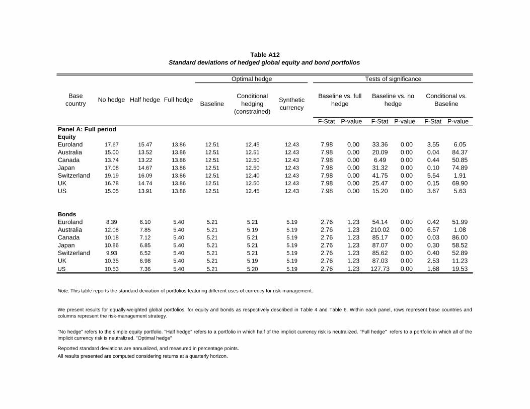
F-Stat P-value F-Stat P-value F-Stat P-valuePanel A: Full periodEquityEuroland 17.67 15.47 13.86 12.51 12.45 12.43 7.98 0.00 33.36 0.00 3.55 6.05Australia 15.00 13.52 13.86 12.51 12.51 12.43 7.98 0.00 20.09 0.00 0.04 84.37Canada 13.74 13.22 13.86 12.51 12.50 12.43 7.98 0.00 6.49 0.00 0.44 50.85Japan 17.08 14.67 13.86 12.51 12.50 12.43 7.98 0.00 31.32 0.00 0.10 74.89Switzerland 19.19 16.09 13.86 12.51 12.40 12.43 7.98 0.00 41.75 0.00 5.54 1.91UK 16.78 14.74 13.86 12.51 12.50 12.43 7.98 0.00 25.47 0.00 0.15 69.90US 15.05 13.91 13.86 12.51 12.45 12.43 7.98 0.00 15.20 0.00 3.67 5.63

BondsEuroland 8.39 6.10 5.40 5.21 5.21 5.19 2.76 1.23 54.14 0.00 0.42 51.99Australia 12.08 7.85 5.40 5.21 5.19 5.19 2.76 1.23 210.02 0.00 6.57 1.08Canada 10.18 7.12 5.40 5.21 5.21 5.19 2.76 1.23 85.17 0.00 0.03 86.00Japan 10.86 6.85 5.40 5.21 5.21 5.19 2.76 1.23 87.07 0.00 0.30 58.52Switzerland 9.93 6.52 5.40 5.21 5.21 5.19 2.76 1.23 85.62 0.00 0.40 52.89UK 10.35 6.98 5.40 5.21 5.19 5.19 2.76 1.23 87.03 0.00 2.53 11.23US 10.53 7.36 5.40 5.21 5.20 5.19 2.76 1.23 127.73 0.00 1.68 19.53

"No hedge" refers to the simple equity portfolio. "Half hedge" refers to a portfolio in which half of the implicit currency risk is neutralized. "Full hedge" refers to a portfolio in which all of theimplicit currency risk is neutralized. "Optimal hedge"

Reported standard deviations are annualized, and measured in percentage points.All results presented are computed considering returns at a quarterly horizon.

Synthetic currency

Baseline vs. full hedge

Baseline vs. no hedge

Conditional vs. Baseline

Note. This table reports the standard deviation of portfolios featuring different uses of currency for risk-management.

We present results for equally-weighted global portfolios, for equity and bonds as respectively described in Table 4 and Table 6. Within each panel, rows represent base countries andcolumns represent the risk-management strategy.

Table A12Standard deviations of hedged global equity and bond portfolios

Base country No hedge Half hedge Full hedge

Optimal hedge Tests of significance

BaselineConditional

hedging (constrained)

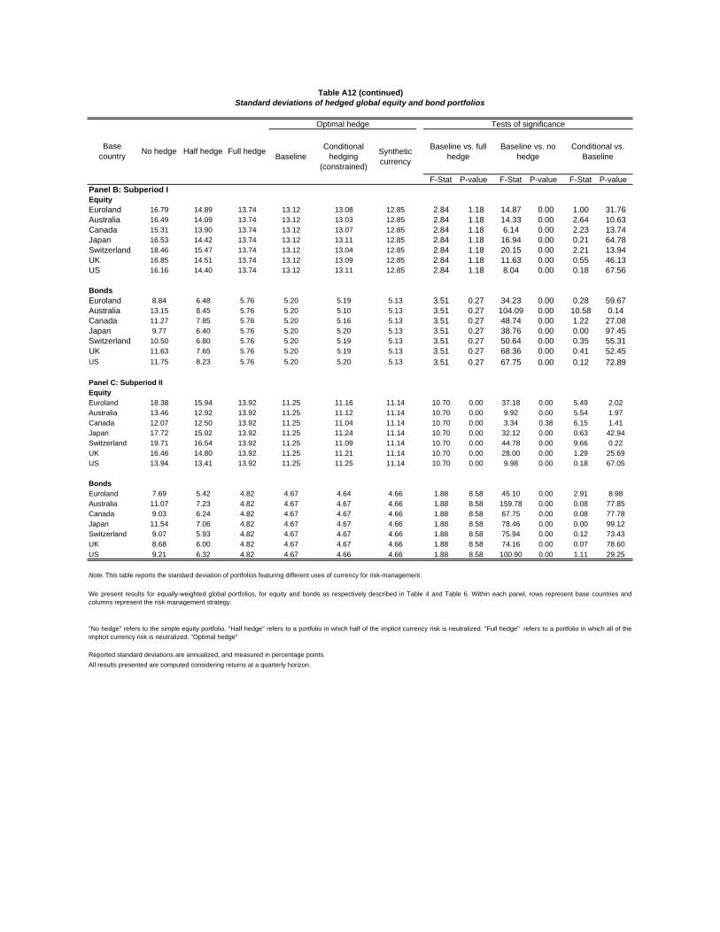
F-Stat P-value F-Stat P-value F-Stat P-valuePanel B: Subperiod IEquityEuroland 16.79 14.89 13.74 13.12 13.08 12.85 2.84 1.18 14.87 0.00 1.00 31.76Australia 16.49 14.09 13.74 13.12 13.03 12.85 2.84 1.18 14.33 0.00 2.64 10.63Canada 15.31 13.90 13.74 13.12 13.07 12.85 2.84 1.18 6.14 0.00 2.23 13.74Japan 16.53 14.42 13.74 13.12 13.11 12.85 2.84 1.18 16.94 0.00 0.21 64.78Switzerland 18.46 15.47 13.74 13.12 13.04 12.85 2.84 1.18 20.15 0.00 2.21 13.94UK 16.85 14.51 13.74 13.12 13.09 12.85 2.84 1.18 11.63 0.00 0.55 46.13US 16.16 14.40 13.74 13.12 13.11 12.85 2.84 1.18 8.04 0.00 0.18 67.56

BondsEuroland 8.84 6.48 5.76 5.20 5.19 5.13 3.51 0.27 34.23 0.00 0.28 59.67Australia 13.15 8.45 5.76 5.20 5.10 5.13 3.51 0.27 104.09 0.00 10.58 0.14Canada 11.27 7.85 5.76 5.20 5.16 5.13 3.51 0.27 48.74 0.00 1.22 27.08Japan 9.77 6.40 5.76 5.20 5.20 5.13 3.51 0.27 38.76 0.00 0.00 97.45Switzerland 10.50 6.80 5.76 5.20 5.19 5.13 3.51 0.27 50.64 0.00 0.35 55.31UK 11.63 7.65 5.76 5.20 5.19 5.13 3.51 0.27 68.36 0.00 0.41 52.45US 11.75 8.23 5.76 5.20 5.20 5.13 3.51 0.27 67.75 0.00 0.12 72.89

Panel C: Subperiod IIEquityEuroland 18.38 15.94 13.92 11.25 11.16 11.14 10.70 0.00 37.18 0.00 5.49 2.02Australia 13.46 12.92 13.92 11.25 11.12 11.14 10.70 0.00 9.92 0.00 5.54 1.97Canada 12.07 12.50 13.92 11.25 11.04 11.14 10.70 0.00 3.34 0.38 6.15 1.41Japan 17.72 15.02 13.92 11.25 11.24 11.14 10.70 0.00 32.12 0.00 0.63 42.94Switzerland 19.71 16.54 13.92 11.25 11.09 11.14 10.70 0.00 44.78 0.00 9.66 0.22UK 16.46 14.80 13.92 11.25 11.21 11.14 10.70 0.00 28.00 0.00 1.29 25.69US 13.94 13.41 13.92 11.25 11.25 11.14 10.70 0.00 9.98 0.00 0.18 67.05

BondsEuroland 7.69 5.42 4.82 4.67 4.64 4.66 1.88 8.58 45.10 0.00 2.91 8.98Australia 11.07 7.23 4.82 4.67 4.67 4.66 1.88 8.58 159.78 0.00 0.08 77.85Canada 9.03 6.24 4.82 4.67 4.67 4.66 1.88 8.58 67.75 0.00 0.08 77.78Japan 11.54 7.06 4.82 4.67 4.67 4.66 1.88 8.58 78.46 0.00 0.00 99.12Switzerland 9.07 5.93 4.82 4.67 4.67 4.66 1.88 8.58 75.94 0.00 0.12 73.43UK 8.68 6.00 4.82 4.67 4.67 4.66 1.88 8.58 74.16 0.00 0.07 78.60US 9.21 6.32 4.82 4.67 4.66 4.66 1.88 8.58 100.90 0.00 1.11 29.25

Baseline vs. full hedgeSynthetic

currency

Conditional hedging

(constrained)

"No hedge" refers to the simple equity portfolio. "Half hedge" refers to a portfolio in which half of the implicit currency risk is neutralized. "Full hedge" refers to a portfolio in which all of theimplicit currency risk is neutralized. "Optimal hedge"

Reported standard deviations are annualized, and measured in percentage points.

Table A12 (continued)Standard deviations of hedged global equity and bond portfolios

Optimal hedge Tests of significance

All results presented are computed considering returns at a quarterly horizon.

Conditional vs. Baseline

Base country

Note. This table reports the standard deviation of portfolios featuring different uses of currency for risk-management.

We present results for equally-weighted global portfolios, for equity and bonds as respectively described in Table 4 and Table 6. Within each panel, rows represent base countries andcolumns represent the risk-management strategy.

Baseline vs. no hedgeBaselineFull hedgeHalf hedgeNo hedge

Slope P-Value Slope P-Value Slope P-Value Slope P-ValueEuroland -0.23 1.00 0.73 0.38 0.02 1.00 -0.24 0.09

(0.62) (2.22) 0.11 0.94Australia 0.00 1.00 0.41 0.10 0.00 1.00 -0.21 0.20

(0.33) (0.68) 0.07 0.28Canada 0.03 1.00 -2.60 0.06 -0.02 1.00 -1.55 0.19

(0.37) (1.98) 0.12 0.88Japan -0.05 0.99 -0.64 0.06 -0.02 1.00 -0.27 0.00

(0.17) (1.45) 0.09 0.49Switz. -0.09 1.00 0.48 0.37 0.00 1.00 -1.01 0.66

(0.48) (1.86) 0.10 0.73UK 0.01 1.00 2.59*** 0.63 0.02 1.00 0.17 0.00

(0.36) (0.97) 0.07 0.43US 0.05 1.00 2.17 0.18 0.00 1.00 0.56 0.49

(0.34) (2.22) 0.11 0.98

Table A13

Optimal conditional currency exposure for an equally-weighted global portfolio: single and multiple - currency case using the real interest rate differential

Note. This table reports optimal currency exposure conditional on real interest rate. For each base country-currency pair, we now let the optimal currency position vary with the log real interest rate differential (ex-post real interest rate of the foreign country minus that of the base country). Yet, we impose the constraints that the slopes of the optimal positions with respect to the interest rate differential be equal across foreign currencies.

The "Multiple Currency" columns consider the case of an investor using all foreign currencies simultaenously to manage risk, but still constrain the slopes to be the same across foreign currencies. Resulting slope coefficients are reported for each base country, followed by the P-value of a test of the constraint. A P-value of x% indicates that the constraint can be rejected at the x% level.

Base Currency

The "Single Currency" columns consider the case of an investor using one currency at a time to manage risk, but still constrain the slopes to be the same across foreign currencies. Resulting slope coefficients from a SUR estimation are reported for each base country, followed by the P-value of a test of the constraint. A P-value of x% indicates that the constraint can be rejected at the x% level.

BondsEquity

Single Currency Single CurrencyMultiple Currencies Multiple Currencies

BaselineConditional

hedging (constrained)

Synthetic currency

Panel A: Full periodEquityEuroland 0.41 0.46 0.51 0.47 0.51 0.54Australia 0.47 0.50 0.47 0.47 0.47 0.54Canada 0.48 0.50 0.47 0.47 0.49 0.54Japan 0.42 0.47 0.48 0.47 0.49 0.54Switzerland 0.45 0.49 0.52 0.47 0.53 0.54UK 0.38 0.45 0.49 0.47 0.48 0.54US 0.53 0.52 0.48 0.48 0.55 0.54

BondsEuroland 0.31 0.41 0.44 0.43 0.45 0.50Australia 0.25 0.35 0.46 0.44 0.41 0.50Canada 0.26 0.36 0.45 0.43 0.44 0.50Japan 0.26 0.38 0.43 0.43 0.46 0.50Switzerland 0.39 0.48 0.44 0.44 0.45 0.50UK 0.20 0.32 0.45 0.43 0.51 0.50US 0.36 0.43 0.46 0.44 0.49 0.50

Table A14Sharpe ratios

Base country No hedge Half hedge Full hedge

Optimal hedge

Note. Table 10 reports Sharpe ratios of portfolios featuring different uses of currency for risk-management. Please refer to Table 9 for a detailed description of these portfolios.

The Sharpe Ratio of each portfolio is calculated as the ratio of the log mean gross return on the portfolio divided by the standard deviation of the log return on the portfolio. Please see Appendix for a detailed description of the calculation of the Sharpe Ratio.

All results presented are computed considering returns at a quarterly horizon.

BaselineConditional

hedging (constrained)

Synthetic currency

Panel B: Subperiod IEquityEuroland 0.51 0.57 0.61 0.53 0.49 0.73Australia 0.61 0.64 0.59 0.54 0.56 0.73Canada 0.54 0.59 0.59 0.53 0.63 0.73Japan 0.41 0.52 0.59 0.53 0.58 0.72Switzerland 0.55 0.60 0.62 0.54 0.41 0.73UK 0.52 0.59 0.60 0.53 0.59 0.73US 0.60 0.62 0.61 0.54 0.50 0.73

BondsEuroland 0.14 0.18 0.19 0.05 0.08 0.20Australia 0.23 0.25 0.20 0.06 0.08 0.21Canada 0.12 0.16 0.20 0.05 0.19 0.20Japan -0.04 0.04 0.16 0.04 0.04 0.19Switzerland 0.25 0.27 0.18 0.06 0.13 0.21UK 0.14 0.18 0.19 0.06 -0.01 0.21US 0.22 0.23 0.22 0.05 0.02 0.20

Panel C: Subperiod IIEquityEuroland 0.32 0.37 0.41 0.39 0.46 0.34Australia 0.32 0.36 0.35 0.39 0.51 0.33Canada 0.42 0.40 0.35 0.39 0.50 0.34Japan 0.43 0.43 0.39 0.40 0.44 0.34Switzerland 0.37 0.40 0.42 0.40 0.48 0.34UK 0.26 0.33 0.39 0.39 0.45 0.33US 0.45 0.43 0.37 0.40 0.43 0.34

BondsEuroland 0.50 0.68 0.74 0.80 0.74 0.84Australia 0.27 0.47 0.77 0.80 0.81 0.84

Canada 0.42 0.60 0.76 0.80 0.79 0.84Japan 0.50 0.67 0.75 0.81 0.80 0.85Switzerland 0.55 0.72 0.75 0.81 0.79 0.84UK 0.28 0.50 0.75 0.79 0.78 0.84US 0.53 0.68 0.76 0.81 0.73 0.85

Full hedge

Optimal hedge

Table 14 (continued)Sharpe ratios

Base country No hedge Half hedge