Global Atmospheric

Change

Updated IPCC report (2007)

• Optional reading

➔ highlighted in 3rd edition of Masters

• http://www.ipcc.ch/ipccreports/ar4-

wg1.htm

➔ The Scientific Basis

➔ If you’re interested, you can read the other

reports too (mitigation, economic impacts,

etc.)

Global Change

• Recent Proclamations

• Earth Atmospheric Structure

• Oxygen Isotopes

➔ 16O and 18O vs. Temperature Record

• Global Temperature and Solar Effects

• Greenhouse Effect

➔ Solar vs. Terrestrial Radiation

➔ Greenhouse Gases

• Global Energy Balance

• Greenhouse Enhancement

➔ Radiative Forcing

➔ Climate Sensitivity

➔ Greenhouse Gases vs. Temperature Record

➔ Global Warming Potential

1

2

3

4

Background Quotes

• “The balance of evidence suggests a

discernable human influence on global

climate.” —Consensus of 2500 scientists involved in the Intergovernmental

Panel on Climate Change, 1995

• “There is new and stronger evidence

that most of the observed warming over

the last 50 years is attributable to

human activities.” —Intergovernmental Panel on Climate Change, 2000, consensus of

~2500 scientists.

• “Most of the observed increase in globally

averaged temperatures since the

mid-20th century is very likely due to the

observed increase in anthropogenic

greenhouse gas concentrations” —Intergovernmental Panel on Climate Change, 2007, consensus of ~2500

scientists

• “Be worried, be very worried” —Time, April 3, 2006

78%

21%

1%

Nitrogen Oxygen Argon

Overview of Earth’s Atmosphere

• Mostly made up of nitrogen

(78%) and oxygen (21%),

followed by Argon (1%).

• Other gases present in

small concentrations:

carbon dioxide (CO2),

nitrous oxide (N2O),

methane (CH4), ozone (O3),

water vapor, CFCs

(chlorofluorocarbons), NOx,

SOx, VOCs.

• Human activities are much more likely to

affect trace gas concentrations than [O2]

and [N2]

• Layers of the atmosphere according to

changes in temperature:

➔ troposphere, stratosphere, mesosphere,

thermosphere

• Atmosphere is well-mixed up to about 85–

90 km altitude, then composition varies

with altitude

5

6

7

8

Troposphere contains 90%

of the mass of the

atmosphere, and it is

generally well mixed, with

mixing time scales from a

few minutes (vertical

mixing in a thunder cloud)

to a year (interhemisphercal

mixing).

The stratosphere is a

stable layer, containing

not quite 10% of the

atmospheric mass.

Defn. Climate: Average temperature, precipitation,

extreme weather events, winds, glaciation, etc., over a

period of decades.

• In order to have a hope of predicting the

future, we study the Earth’s temperature

in the past.

• Climatologists study tree rings, ice

volume (i.e. markers of glaciation),

fossil pollen, and oxygen isotopes to try

and figure out the past temperature

record.

Global Temperature

Oxygen Isotopes

• Water evaporating from sea has H218O

and H216O

➔ H218O is heavier, and it evaporates

somewhat less readily.

➔ This is called an “isotope effect”, and is very

common in both physical and chemical

processes—i.e. that the rate of a physical

process or a chemical reaction will be

slightly slower for a molecule containing the

heavier isotope.

• The “heavy water” also precipitates very

slightly faster than H216O

• Precipitation that travels as far as the

polar ice sheets is relatively more

depleted in 18O, leaving the sea enriched

in 18O

• The more ice, the more the sea is

enriched in 18O (particularly at the

surface, where the critters are)

9

10

11

12

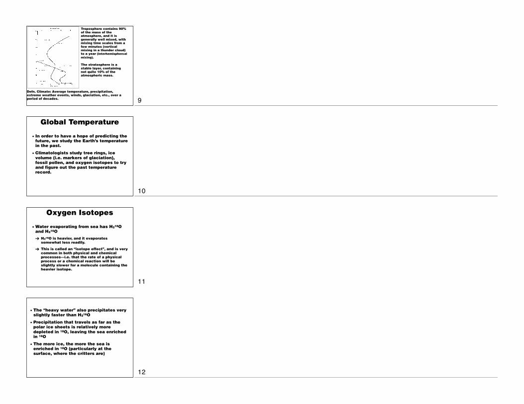
Sea creatures are enriched in 18O ~equivalent

to the level in ocean water.

By measuring the 18O/16O ratio, in the shells left

by diatoms (and dating them with another

stable isotope), we can find the temperature

history of the Earth.

Negative numbers—sample is “depleted”

Positive numbers—sample is “enriched”

Colder temperatures make the δ18Ο + or – in the

ocean?

(Opposite in ice deposits)

δ 18O ‰( ) =18O 16O( )sample − 18O 16O( )standard

18O 16O( )standard

18O in Ice Cores

• As world ice increases, 18O is selectively

removed at the poles. In the same way, the

global temperature can be derived from the

ice in polar ice cores (up to 3 km long!).

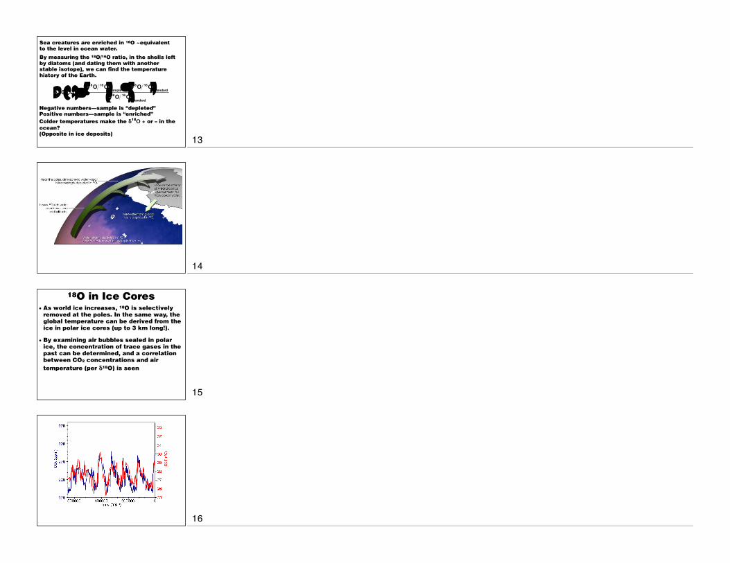
• By examining air bubbles sealed in polar

ice, the concentration of trace gases in the

past can be determined, and a correlation

between CO2 concentrations and air

temperature (per δ18O) is seen

13

14

15

16

• In recent years, the temperature record is

from instruments, carefully calibrated for

technique, urban heat island effect, etc.

(more later)

• Over the last million years, mid-latitude

temperatures have oscillated between 9

and 16°C

• The fastest globally averaged temperature

changes ever have been 1°C/century

• Right now we are looking at best guess

climate change of 2°C by 2100, with a range

of 1.4 to 5.8°C. Temperatures went up last

century by 0.6°C

Global Temperature Change

• Tilt and orbit of the planet

➔ These Milankovitch cycles change aspects

of our orbit with 100000, 41000 and 23000

year periods.

➔ There is a 100000 year cycle between

glaciations, and the other cycles are

observed as well, more or less. The sunlight

only changes by 0.1%!

• Sunspot cycles

➔ The sun has an 11-year cycle in the number

of sunspots

➔ More sunspots (which are cool) are

associated with more faculae (which are

brighter) results in ~0.1 % more sunlight at

the maximum of the cycle. Note the

difference in effect of a long term 0.1%

change and a short term one (2000–2001 was

another solar maxima)

• Shift in ocean and atmospheric

circulation patterns

• To predict the extremely complex effect

of changes in CO2 concentrations

researchers use general circulation

models, but the starting point is a model

that describes how radiation and the

Earth interact.

• Recall: A blackbody absorbs all of the

radiation that impinges upon it

• Energy is emitted from a blackbody

according to its temperature (Stefan-

Boltzmann Law)

Greenhouse Effect

17

18

19

20

• Some of the incoming radiation is

reflected off of the Earth’s surface and it

does not contribute to the Earth’s

warming (albedo)

• From radiative equilibrium principles and

Stefan-Boltzmann Law, we calculated a

terrestrial radiative temperature of about

255 K

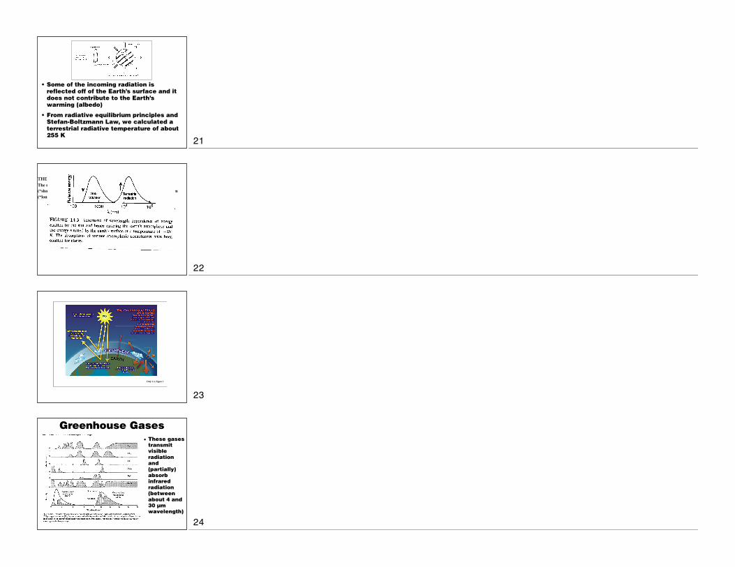
THE GREENHOUSE EFFECT The radiation emitted by the sun is primarily between 0.15 and 3 µm (“short wave”). The radiation emitted by the Earth is between 3 and 80 µm (“long wave”).

FAQ 1.3, Figure 1

• These gases

transmit

visible

radiation

and

(partially)

absorb

infrared

radiation

(between

about 4 and

30 µm

wavelength)

Greenhouse Gases

21

22

23

24

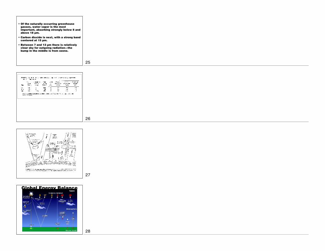
• Of the naturally occurring greenhouse

gasses, water vapor is the most

important, absorbing strongly below 8 and

above 18 µm.

• Carbon dioxide is next, with a strong band

centered at 15 µm.

• Between 7 and 12 µm there is relatively

clear sky for outgoing radiation—the

bump in the middle is from ozone.

Global Energy Balance

25

26

27

28

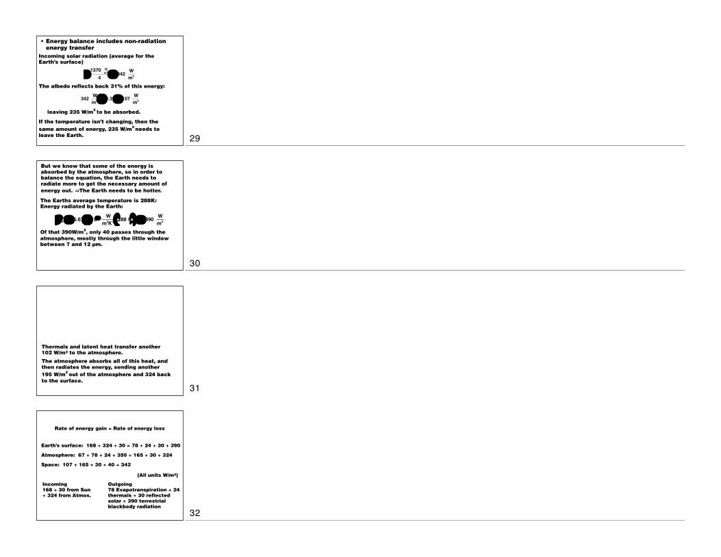
Incoming solar radiation (average for the

Earth’s surface)

The albedo reflects back 31% of this energy:

leaving 235 W/m2

to be absorbed.

If the temperature isn’t changing, then the

same amount of energy, 235 W/m2

needs to

leave the Earth.

• Energy balance includes non-radiation

energy transfer

=1370 W

m2

4= 342 W

m2

342 Wm2 × 0.31 = 107 W

m2

The Earths average temperature is 288K:

Energy radiated by the Earth:

Of that 390W/m2, only 40 passes through the

atmosphere, mostly through the little window

between 7 and 12 µm.

But we know that some of the energy is

absorbed by the atmosphere, so in order to

balance the equation, the Earth needs to

radiate more to get the necessary amount of

energy out. ⇒The Earth needs to be hotter.

σTs4 = 5.67 × 10−8 W

m2K4 288 K( )4 = 390 Wm2

Thermals and latent heat transfer another

102 W/m2 to the atmosphere.

The atmosphere absorbs all of this heat, and

then radiates the energy, sending another

195 W/m2

out of the atmosphere and 324 back

to the surface.

Earth’s surface: 168 + 324 + 30 = 78 + 24 + 30 + 390

Atmosphere: 67 + 78 + 24 + 350 = 165 + 30 + 324

Space: 107 + 165 + 30 + 40 = 342

Rate of energy gain = Rate of energy loss

(All units W/m2)

Incoming

168 + 30 from Sun

+ 324 from Atmos.

Outgoing

78 Evapotranspiration + 24

thermals + 30 reflected

solar + 390 terrestrial

blackbody radiation

29

30

31

32

If the system is perturbed by adding radiative

forcing, F (W/m2), then the former equation,

Qabs = Qrad

becomes (at a new equilibrium):

Qabs + ΔQabs + ΔF = Qrad + ΔQrad

ΔF = ΔQrad – ΔQabs

ΔF from changes in:

Greenhouse gas

concentrations

Aerosols

Albedo

Solar constant

Enhancement of Greenhouse Effect

Climate sensitivity parameter

ΔTs = λΔF

λ = the climate sensitivity parameter

Ts = surface temperature (K)

ΔF = forcing in W/m2

Which can also be written in incremental

form (δT, etc.).

Climate Sensitivity

λ =ΔTsΔF

=ΔTs

ΔQrad − ΔQabs=

ΔQrad

ΔTs−

ΔQabs

ΔTs⎛⎝⎜

⎞⎠⎟

−1

• Climate sensitivity depends on:

➔ How much the outgoing radiation at the top

of the atmosphere changes (ΔQrad/ΔTs) as

the surface temperature changes, and

➔ The change of incoming energy that is

absorbed as the surface temperature

changes (ΔQabs/ΔTs)

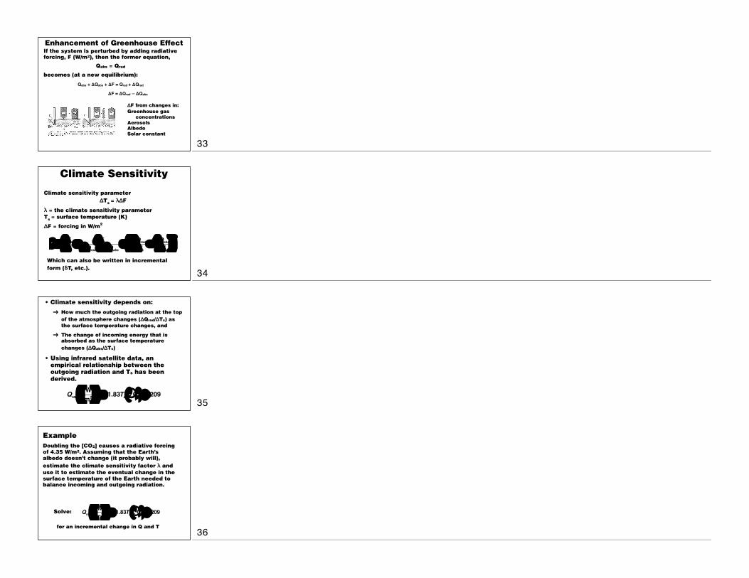
• Using infrared satellite data, an

empirical relationship between the

outgoing radiation and Ts has been

derived.

QradWm2

⎛⎝⎜

⎞⎠⎟

= 1.83Ts °C( ) + 209

Example

Doubling the [CO2] causes a radiative forcing

of 4.35 W/m2. Assuming that the Earth’s

albedo doesn’t change (it probably will),

estimate the climate sensitivity factor λ and

use it to estimate the eventual change in the

surface temperature of the Earth needed to

balance incoming and outgoing radiation.

Solve:

for an incremental change in Q and T

QradWm2

⎛⎝⎜

⎞⎠⎟

= 1.83Ts °C( ) + 209

33

34

35

36

To get the change of T with Q we just need

the slope of this equation,

Since we are assuming the albedo doesn’t

change,

So this approximation of the climate sensitivity

factor is:

ΔQrad

ΔTs= 1.83

ΔQabs

ΔTs= 0

λ =ΔQrad

ΔTs−

ΔQabs

ΔTs

⎛⎝⎜

⎞⎠⎟

−1

= 1.83−1 = 0.55 °CW/m2

The climate sensitivity factor, λ, is quite

uncertain. The IPCC 1995 estimates are from

0.34 to 1.03, with the best guess of 0.57.

If doubling CO2

creates a radiative forcing

of 4.35 W/m2, then

ΔTs = λΔF = 0.55 °CW/m2 × 4.35 W

m2 = 2.4°C

Torn, M. and J. Harte, Geophysical Research Letters, May 26, 2006:

“We quantified this feedback for CO2 and CH4 by combining the mathematics of feedback with empirical ice-core information and general circulation model (GCM) climate sensitivity, finding that the warming of 1.5–4.5°C associated with anthropogenic doubling of CO2 is amplified to 1.6–6.0°C warming, with the uncertainty range deriving from GCM simulations and paleo temperature records. Thus, anthropogenic emissions result in higher final GhG concentrations, and therefore more warming, than would be predicted in the absence of this feedback.”

Scheffer, M., V. Brovkin, and P.M. Cox, Geophysical Research Letters, May 26, 2006:

”…we suggest that the feedback of global temperature on atmospheric CO2 will promote warming by an extra 15–78% on a century-scale. This estimate may be conservative as we did not account for synergistic effects of likely temperature moderated increase in other greenhouse gases.”

Positive forcings warm the Earth, negative

forcings cool the Earth

Figure SPM.2

Fig. 8.29

37

38

39

40

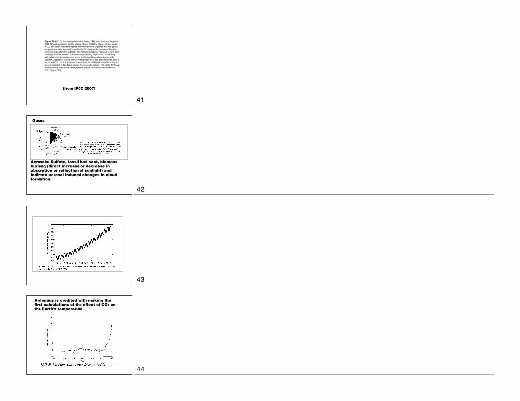
(from IPCC 2007)

Figure SPM.2. Global average radiative forcing (RF) estimates and ranges in2005 for anthropogenic carbon dioxide (CO2), methane (CH4), nitrous oxide(N2O) and other important agents and mechanisms, together with the typicalgeographical extent (spatial scale) of the forcing and the assessed level ofscientific understanding (LOSU). The net anthropogenic radiative forcing andits range are also shown. These require summing asymmetric uncertaintyestimates from the component terms, and cannot be obtained by simpleaddition. Additional forcing factors not included here are considered to have avery low LOSU. Volcanic aerosols contribute an additional natural forcing butare not included in this figure due to their episodic nature. The range for linearcontrails does not include other possible effects of aviation on cloudiness.{2.9, Figure 2.20}

Aerosols: Sulfate, fossil fuel soot, biomass

burning (direct increase or decrease in

absorption or reflection of sunlight) and

indirect: aerosol induced changes in cloud

formation.

Gases

Arrhenius is credited with making the

first calculations of the effect of CO2 on

the Earth’s temperature

41

42

43

44

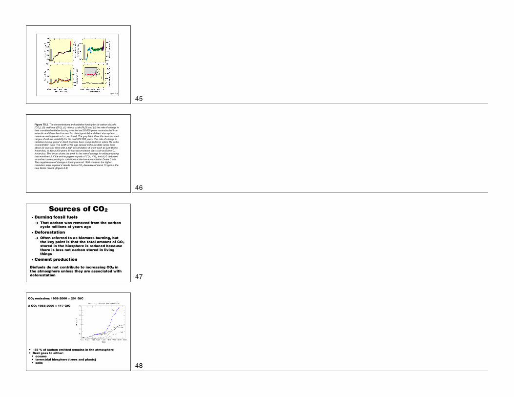
Figure TS.2

Figure TS.2. The concentrations and radiative forcing by (a) carbon dioxide(CO2), (b) methane (CH4), (c) nitrous oxide (N2O) and (d) the rate of change intheir combined radiative forcing over the last 20,000 years reconstructed fromantarctic and Greenland ice and firn data (symbols) and direct atmosphericmeasurements (panels a,b,c, red lines). The grey bars show the reconstructedranges of natural variability for the past 650,000 years. The rate of change inradiative forcing (panel d, black line) has been computed from spline fits to theconcentration data. The width of the age spread in the ice data varies fromabout 20 years for sites with a high accumulation of snow such as Law Dome,Antarctica, to about 200 years for low-accumulation sites such as Dome C,Antarctica. The arrow shows the peak in the rate of change in radiative forcingthat would result if the anthropogenic signals of CO2, CH4, and N2O had beensmoothed corresponding to conditions at the low-accumulation Dome C site.The negative rate of change in forcing around 1600 shown in the higher-resolution inset in panel d results from a CO2 decrease of about 10 ppm in theLaw Dome record. {Figure 6.4}

Sources of CO2

• Burning fossil fuels

➔ That carbon was removed from the carbon

cycle millions of years ago

• Deforestation

➔ Often referred to as biomass burning, but

the key point is that the total amount of CO2

stored in the biosphere is reduced because

there is less net carbon stored in living

things

• Cement production

Biofuels do not contribute to increasing CO2 in

the atmosphere unless they are associated with

deforestation

CO2 emission: 1958-2000 = 201 GtC

Δ CO2 1958-2000 = 117 GtC

• ~58 % of carbon emitted remains in the atmosphere

• Rest goes to either:

• oceans

• terrestrial biosphere (trees and plants)

• soils

45

46

47

48

The numbers in the boxes are the amount of

carbon in that reservoir, in gigatons (109 tonnes

or 1012 kg).

Anthropogenic emissions are ~5.5 Gt/yr from

fossil fuels and a little cement, ~1.6 Gt/yr from

deforestation in the tropics.

This is offset by about 2 Gt/yr uptake into the

oceans, 0.5 Gt/year re-growth of Northern

forests, and 1.3 Gt/yr other sinks—increased

plant growth from nitrogen and CO2 fertilization

Net storage in the atmosphere:

The airborne fraction is to a degree a function

of the rate of emissions. If the same net

emissions are added over a longer time period,

the ocean and plants have more time to absorb

the carbon, and the airborne fraction is lower;

possibly 35%

49

50

51

52

Methane

Has more than doubled since pre-industrial times.

Methane has many sources:

Methane is removed by reacting with our old

friend the OH radical:

CH4 + OH + O2 → H2O + HCHO + HO2

HCHO + OH + O2 → HO2 + CO + H2O

CO + OH + O2 → CO2 + HO2

• Net reduction of [OH] after reaction with

methane

➔ Results in increased [CH4]

• Global warming could free large amounts

of methane from permafrost and provide

another positive feedback loop.

• A large enough temperature increase may

cause CH4 release from methane

clathrates in the ocean

N2O is produced in nitrification reactions—

either by bacteria or in fertilizer production:

NH4+ → N2 → N2O → NO2- → NO3-

Nitrous Oxide (N2O)

53

54

55

56

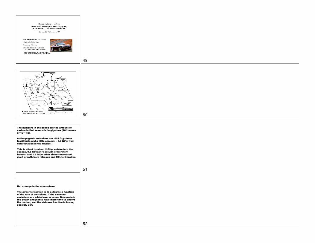
Halocarbons

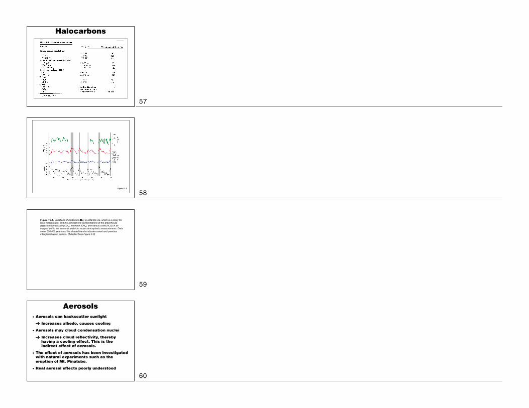
Figure TS.1

Figure TS.1. Variations of deuterium ( D) in antarctic ice, which is a proxy forlocal temperature, and the atmospheric concentrations of the greenhousegases carbon dioxide (CO2), methane (CH4), and nitrous oxide (N2O) in airtrapped within the ice cores and from recent atmospheric measurements. Datacover 650,000 years and the shaded bands indicate current and previousinterglacial warm periods. {Adapted from Figure 6.3}

Aerosols

• Aerosols can backscatter sunlight

➔ Increases albedo, causes cooling

• Aerosols may cloud condensation nuclei

➔ Increases cloud reflectivity, thereby

having a cooling effect. This is the

indirect effect of aerosols.

• The effect of aerosols has been investigated

with natural experiments such as the

eruption of Mt. Pinatubo.

• Real aerosol effects poorly understood

57

58

59

60

Global Warming Potential

• Gases contribute to the greenhouse

effect if they absorb in the 7–12 µm

window where natural greenhouse

gasses have not already saturated the

bands.

• If an absorber only adds to the “wings”

of an absorption band, and most of the

band is already saturated, then it will

not be so effective on a per-molecule

basis.

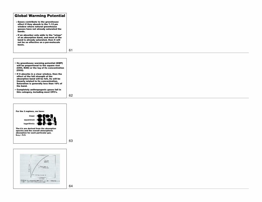
• Its greenhouse warming potential (GWP)

will be proportional to the square root

(CH4, N2O) or the log of its concentration

(CO2).

• If it absorbs in a clear window, then the

effect of the full strength of the

absorption band will be felt, its will be

linearly related to its concentration.

Saturation is generally less than 10% of

the band.

• Completely anthropogenic gases fall in

this category, including most CFC’s.

For the 3 regimes, we have:

The k’s are derived from the absorption

spectra and the overall atmospheric

absorption for each particular gas.

kCO2 = 6.3.

linear: F = k1 C − C0( )squareroot: F = k2 C − C0( )logarithmic: F = k3 lnC − lnC0( )

61

62

63

64

65