Global Atlas of environmental parameters for chemical fate...

EUR 24255 EN - 2010

Global Atlas of environmentalparameters for chemical fate and

transport assessment

Grazia Zulian, Paolo Isoardi, Alberto Pistocchi

2

The mission of the JRC-IES is to provide scientific-technical support to the European Union’s policies for the protection and sustainable development of the European and global environment. European Commission Joint Research Centre Institute for Environment and Sustainability Contact information Address: Grazia Zulian, JRC, TP 460, Via Enrico Fermi 2749, 21027 Ispra (VA), Italy E-mail: [email protected] Tel.: +390332783099 Fax: +390332785601 http://ies.jrc.ec.europa.eu/ http://www.jrc.ec.europa.eu/ Legal Notice Neither the European Commission nor any person acting on behalf of the Commission is responsible for the use which might be made of this publication.

Europe Direct is a service to help you find answers to your questions about the European Union

Freephone number (*):

00 800 6 7 8 9 10 11

(*) Certain mobile telephone operators do not allow access to 00 800 numbers or these calls may be billed.

A great deal of additional information on the European Union is available on the Internet. It can be accessed through the Europa server http://europa.eu/ JRC 59846 EUR 24255 EN ISBN 978-92-79-15025-8 ISSN 1018-5593 doi:10.2788/63436 Luxembourg: Publications Office of the European Union © European Union, 2010 Reproduction is authorised provided the source is acknowledged Printed in Italy

3

Table of Contents 1. Introduction............................................................................................................................ 5

2. Data catalog: Soil................................................................................................................... 5

2.1 OC content and bulk density.............................................................................................. 5 2.2 Soil Texture........................................................................................................................ 8 2.3 Soil moisture storage capacity ......................................................................................... 11 2.4 Runoff .............................................................................................................................. 13 2.5 Sediments removal rate for basin .................................................................................... 14

3. Data catalog: atmosphere.................................................................................................... 18

3.1 ABL mixing height............................................................................................................ 18 3.2 Temperature .................................................................................................................... 19 3.3 Wind Speed ..................................................................................................................... 21 3.4 Precipitation..................................................................................................................... 22 3.5 SnowFall .......................................................................................................................... 24 3.6 Aerosol ............................................................................................................................ 25

4. Data Catalog: Stream Network ............................................................................................ 30

4.1 Networks.......................................................................................................................... 30 4.2 Potential Simulated Topological Networks....................................................................... 33 4.3 Global Lakes.................................................................................................................... 34 4.4 Average Residence Time (ART) of Pollutants in Inland Surface Water ........................... 36

5. Data Catalog: Oceans ......................................................................................................... 41

5.1 Temperature .................................................................................................................... 41 5.2 Salinity ............................................................................................................................. 42 5.3 Mixed layer depth ............................................................................................................ 43 5.4 Chlorophyll....................................................................................................................... 44 5.5 Surface velocity ............................................................................................................... 46 5.6 Water surfaces................................................................................................................. 48

6. Data Catalog: Vegetation..................................................................................................... 49

6.1 Vegetation ....................................................................................................................... 49 7. Data Catalog: Antrophic Factors.......................................................................................... 52

4

7.1 World stable lights ........................................................................................................... 52 7.2 Population counts, population density ............................................................................. 54 7.1 Impervious Surface Area ................................................................................................. 56

8. Softwares............................................................................................................................. 60

8.1.1 Arcgis 9.x .................................................................................................................. 60 8.1.2 Panoply ..................................................................................................................... 60 8.1.3 NCO operators .......................................................................................................... 60 8.1.4 Ilwis 3.3 ..................................................................................................................... 60 8.1.5 HDF........................................................................................................................... 60

9. Annex A - Data mining from the online World Lake Database ............................................. 61

9.1 Mean depth...................................................................................................................... 66 9.2 GLWD integration ............................................................................................................ 66

10. Annex B - Estimation of parameters to predict mean lake depth on a global scale. ............ 67

10.1.1 Conversion of Hydro1k dataset to GRID format ...................................................... 67 10.1.2 Calculation of parameters ....................................................................................... 67 10.1.3 Analysis of parameters............................................................................................ 68 10.1.4 Regression analysis ................................................................................................ 72 10.1.5 Conclusions ............................................................................................................ 78

10.2 Application of the Slope-area model on global scale. .................................................. 78 10.3 References .................................................................................................................. 78

11. Acknowledgements.............................................................................................................. 79

Global atlas of environmental parameters

5

1. Introduction

This report describes the construction, formatting and analysis of global data retrieved with the purpose to parameterize the global spatial model of chemical fate and transportation. Such model is described in a companion report (Pistocchi e al. 2010). The data collection concerns the atmosphere, soils, the strean network and lakes, and the ocean; besides environmental media, factors representing anthropic activity are also included, which are an indicator of both potential chemical emissions, and potential exposure. Most of the data were readily available and needed simple reformatting and organization in the database. Some datasets were generated by models run in different contexts, such as the ones about atmospheric aerosol and deposition. Most of the datasets were originally in time series and required averaging monthly and annual values. A few datasets were generated specifically for the present atlas: notably the residence time of inland surface waters, sediment yields from catchments, and ocean particulate organic matter and sinking fluxes, which were derived using specific regression equations. In the report, all details concerning each dataset are presented along with discussion on the methods used for original datasets. The need to provide also rather technical metadata justifiesthe schematic organization of the text in most sections of the report. References given for each data set provide additional information. The data set is available in a collection of GIS files organized as indicated for each theme hereafter; the datasets are available upon request, subject to conditions of use to be established by the JRC. Data can be downloaded from the JRC FATE Web sites http://fate.jrc.ec.europa.eu/rational/home

2. Data catalog: Soil

2.1 OC content and bulk density DATA SOURCE ISRIC - World Soil Information ORIGINAL DATA DESCRIPTION ISRIC-WISE derived soil properties on a 5 by 5 arc-minutes global grid (ver. 1.1).

This harmonized, global data set was prepared using: spatial data from the 1:5 million scale FAO-Unesco Soil Map of the Word and soil parameter estimates derived from ISRIC’s WISE database.

The data set includes derived soil properties for the 106 soil units shown on the Soil Map of the World, for fixed depth intervals of 20 cm up to 100 cm depth.

The soil variables under consideration are: drainage class, organic carbon content (g kg -1), total nitrogen, C/N ratio, pH(H2O), CECsoil, CECclay, effective CEC, base saturation, aluminum saturation, calcium carbonate content, gypsum content, exchangeable sodium percentage (ESP), electrical conductivity, particle size distribution (i.e. content of sand, silt and clay), content of coarse fragments, bulk density (kg dm -3), and available water capacity (-33 to -1500 kPa).

Modal values shown for the derived soil properties should be seen as 'best' estimates; possible types and sources of uncertainty are discussed in the documentation.


6

The GIS project file includes selected binned data sets, as examples of possible output; these classified data consider the full map unit composition. The data set also includes several other tables, listing derived soil parameters by soil unit and depth layer, which can be joined to the raster data using GIS. These include both binned and un-binned data.

SOURCE CITATION Batjes NH 2006. ISRIC-WISE derived soil properties on a 5 by 5 arc-minutes

global grid. Report 2006/02 (available through http://www.isric.org), ISRIC – World Soil Information, Wageningen (with data set)

DOWNLOAD LINK http://www.isric.org/UK/About+Soils/Soil+data/Geographic+data/Global/WISE5

by5minutes.htm ACCESSED 18/07/2008 SPATIAL RESOLUTION 5’x5’, 1°x1° PRIMARY DATA FORMAT GRID file smw5by5min PROCESSING Import of original GRID file smw5by5min into “File GeoDatabase Raster

Dataset” format; resample to 1 by1sec resolution. Reclass using the central values of classes. STORED IN \\globaldata\soil\Bulk \\globaldata\soil\OC


7

Figure 1: Bulk density


8

2.2 Soil Texture DATA SOURCE Oak Ridge National Laboratory Distributed Active Archive Center (ORNL

DAAC) ORIGINAL DATA DESCRIPTION A standardized global data set of soil horizon thicknesses and textures (particle

size distributions) was compiled by Webb et al. This data set will be used for the improved ground hydrology parameterization design for the Goddard Institute for Space Studies General Circulation Model (GISS GCM) Model III. The data set specifies the top and bottom depths and the percent abundance of sand, silt, and clay of individual soil horizons in each of the 106 soil types cataloged for nine continental divisions. When combined with the World Soil Data File (Zobler, 1986), the result is a global data set of variations in physical properties throughout the soil profile. These properties are important in the determination of water storage in individual soil horizons and exchange of water with the lower atmosphere. The incorporation of this data set into the GISS GCM should improve model performance by including more realistic variability in land-surface properties.

All data are global at a 1 degree resolution and are provided in ASCII format. The profile data are also offered in ESRI export file format. The primary data consist of depth and particle size (percent sand, silt, and clay) information for each major continent, soil type, and soil horizon. Ocean/continental coding (corresponding to FAO/UNESCO Soil

Figure 2: Organic Carbon Content.


9

Map of the World) (FAO/UNESCO, 1971-1981) and Zobler soil type classifications (Zobler, 1986) are also included. In addition to the primary data files, there are also four derived data sets available for download: (1) data on potential storage of water in the soil profile, (2) data on potential storage of water in the root zone, (3) data on potential storage of water derived from soil texture, and (4) a data set used to prescribe water-holding capacity in the GISS GCM (Model II).

There are 15 global grids included in this data set. Each grid represents a soil

horizon (named profile*m), with profile1m representing the horizon closest to the soil surface and profile15m representing the deepest horizon possible. No soil type within this data set contained more than 14 horizons. However, empty records were retained and flagged with a value of -1. For example, if a given soil type contained 13 soil horizons, the first grid (profile1m) would record a depth of 0 and the corresponding sand, silt, and clay proportions for the first horizon, the second grid (profile2m) would record the contact depth of the second horizon as well as the proportion sand, silt, and clay for the second horizon, and so on. The thirteenth grid (profile13m) would record the contact depth of the thirteenth horizon and the proportion sand, silt, and clay for the thirteenth (and final) horizon, and the fourteenth grid (profile14m) would record the depth of the BOTTOM of the thirteenth horizon and carry the flagged value of -1 for the values of sand, silt, and clay. The fifteenth grid (profile15m) would carry the flagged value of -1 for the depth, sand, silt, and clay attributes.

Table 1: Soil Texture attributes.

Code Soil Moisture Capacity

VALUE an arbitrary but unique identifier assigned during the creation of the grid

COUNT the number of cells within the grid assigned to a given VALUE

CONTNGDC continent code (1‐10)

ZOBLER_106 Zobler soil type

UNIQUE_ID a key‐id created by combining the CONTNGDC_ZOBLER_106

DEPTH* soil depth (meters); the first value is 0 for a given soil type

SAND* percent sand for a given horizon

SILT* percent silt for a given horizon

CLAY* percent clay for a given horizon

SOURCE CITATION Webb, R. W., C. E. Rosenzweig, and E. R. Levine. 2000. Global Soil Texture and

Derived Water-Holding Capacities (Webb et al.). Data set. Available on-line (http://www.daac.ornl.gov) from Oak Ridge National Laboratory Distributed Active Archive Center, Oak Ridge, Tennessee, U.S.A. doi:10.3334/ORNLDAAC/548.

LINK http://daac.ornl.gov/SOILS/guides/Webb.html ACCESSED


10

21/07/2008 SPATIAL RESOLUTION 1°x1° TEMPORAL RESOLUTION --- PRIMARY DATA FORMAT *.e00 file PROCESSING Import of original e00 files into “File GeoDatabase Raster Dataset” format STORED IN \\globaldata\soil\Texture Figure 3: example map from the soil texture data set: percentage of sand at 2 m depth


11

2.3 Soil moisture storage capacity DATA SOURCE FAO-UNESCO Soil Map of the World ORIGINAL DATA DESCRIPTION The raster dataset of soil moisture storage capacity has a spatial resolution of 5 *

5 arc minutes and is in geographic projection. Information with regard to soil moisture was obtained from the "Derived Soil Properties" of the FAO-UNESCO Soil Map of the World which contains raster information on soil properties.

This parameter indicates the amount of soil moisture that can be stored between field capacity and wilting point and is presumed to be available to plants. It is calculated on the basis of soil depth and textural class. The dataset is available for download (below) in both ASCII and ESRI GRID formats. A layer (.lyr) legend (.avl) and excel file are provided in the downloads.

Structure of the attributes: The first digit indicates the dominant Smax class (60% of the cell). The second

digit indicates the associated (40% of the cell) class. When the second number is 0, this indicates that the whole cell is made up by the Smax class indicated by the first number. Soil Moisture Capacity -- The classes are: 1: Wetlands 2: > 200 mm/m 3: 150 - 200 mm/m 4: 100 - 150 mm/m 5: 60 - 100 mm/m 6: 20 - 60 mm/m 7: < 20 mm/m 97:Water 99:Glaciers, Rock, Shifting sand, Missing data

SOURCE CITATION FAO/UNESCO. Digital Soil Map of the World and Derived Soil Properties. Rev.

1. (CD Rom), 2003. Available from http://www.fao.org/catalog/what_new-e.htm (interactive catalogue).

LINK http://www.fao.org/geonetwork/srv/en/resources.get?id=30576&fname=smax.zip

&access=private http://www.fao.org/geonetwork/srv/en/metadata.show?id=30576 ACCESSED 21/07/2008 SPATIAL RESOLUTION 5’x5’, 1°x1° TEMPORAL RESOLUTION --- PRIMARY DATA FORMAT *.mdb


12

PROCESSING Import of original files into “File GeoDatabase Raster Dataset” format; resample

to 1by1sec resolution. Reclass following the structure of the attribute table.

The first digit indicates the dominant Smax class (60% of the cell). The second digit indicates the associated (40% of the cell) class. When the second number is 0, this indicates that the whole cell is made up by the Smax class indicated by the first number.

Table 2: structure of the attribute table

Code Soil Moisture Capacity 1 Wetlands 2 > 200 mm/m 3 150 ‐ 200 mm/m 4 100 ‐ 150 mm/m 5 60 ‐ 100 mm/m 6 20 ‐ 60 mm/m 7 < 20 mm/m 8 Water 9 Glaciers, Rock, Shifting sand, Missing data 10 Wetlands

STORED IN \\globaldata\soilmoisture\soilmoisture Figure 4: Soil Moisture storage capacity.


13

2.4 Runoff DATA SOURCE UNH-GRDC Global Composite Runoff Fields ORIGINAL DATA DESCRIPTION The present data set demonstrates the potential of combining observed river

discharge information with a climate-driven Water Balance Model in order to develop composite runoff fields which are consistent with observed discharges. Such combined runoff fields preserve the accuracy of the discharge measurements as well as the spatial and temporal distribution of simulated runoff, thereby providing the "best estimate" of terrestrial runoff over large domains.

Runoff Field Data Structures Three sets of annual and monthly climatological (1+12 layers per set) runoff

fields are included on the accompanying CD-ROM. The sets are observed, WBM-simulated, and composite monthly runoff fields in the ./arc/w_runoff ARC/INFO workspace and ./ascii/runoff directory. The grid coverage names are g_obs_ro01, g_obs_ro02, ..., g_obs_ro12 and g_obs_ro, where the numbered coverages are the monthly values and g_obs_ro contains the annual sum of the observed runoffs. The WBM simulated and the composite fields are organized similarly in g_wbm_ro## and g_cmp_ro## coverages. The same grid coverages are given as ARC/INFO ASCII grids as well in the ./ascii/runoff directory using the same naming convention (obs_ro##.grd, wmb_ro##.grd and cmp_ro##.grd). The monthly runoff values are given in mm/mo at 30-minute (0.5 degree) spatial resolution. The annual values are given in mm/yr.

SOURCE CITATION Fekete, B.M., Vo¨ro¨smarty, C.J., Grabs, W., 1999. Global composite runoff

fields of observed river discharge and simulated water balances. Report No. 22, Global Runoff Data Centre, Koblenz, Germany.

LINK http://www.grdc.sr.unh.edu/ ACCESSED 15/07/2008 SPATIAL RESOLUTION 0.5°x 0.5° UNIT mm/yr PROCESSING Import of original cmp_ro.asc file into “File GeoDatabase Raster Dataset” format.


14

STORED IN \\globaldata\soil\Run_Off\run_off

Figure 5: Runoff

2.5 Sediments removal rate for basin

DATA SOURCE Inputs:

- Basins: H1K (for each Continent) - Elevation: H1K (global) - Run Off: (global) - Temperature : global monthly means

SPATIAL RESOLUTION 1km x 1km (0.008333° x 0.008333°) PROCESSING Modified Syvitski model kg/s/m2


15

BRIEF DESCRIPTION OF THE MODEL ADOPTED TOGENERATE THE DATASET the total sediment yield from a catchment’s unit area in kg s-1m-2 is computed

according to the model proposed by Syvitski et al., 2000 (see also Pistocchi, 2008): 5.05.1 −Δ= AQs αϕ

where A is the catchment area in km2, and H is the basin relief (defined as the maximum elevation above catchment outlet) in m, α is a coefficientaccounting for the catchment climate, and ϕ is a parameter, not included in the original model, which is added here to account for the actual capacity of the catchment hydrology to deliver sediments.

The parameter α is suggested to be equal to 2 x 10-5 for temperate climates, and 10-6 for cold catchments (Syvitski et al., 2000). We represented this parameter through a fuzzy membership function in the form shown in Figure 6.

The function is a simple transformation of the map of mean annual temperature [temp_avg], which is obtained through the following map algebra statement (ESRI ArcGIS ® syntax):

[alfa]= Con([temp_avg] >= 278, 0.00002, Con([temp_avg] <= 273, 0.000001, 0.000001 + ([temp_avg] - 273) / (278 - 273) * (0.00002 - 0.000001))

The capacity of a catchment to actually deliver sediments depends on its average runoff generation. We assume that ϕ is valued 1 whenever runoff [runoff_composite_annual] exceeds 100 mm, and 0 when it is below 25 mm. In between, a linear variation is assumed (Figure 7). This can be obtained through a map algebra statement as follows:

[phi]=Con([runoff_composite_annual] >= 100,1,

Con([runoff_composite_annual] <= 25, 0, [runoff_composite_annual] / 100))

0.0E+00

5.0E-06

1.0E-05

1.5E-05

2.0E-05

-25 -20 -15 -10 -5 0 5 10 15

mean annual temperature oC

α

Figure 6 – α as a function of mean annual temperature of the catchment.


16

0.0E+00

2.0E-01

4.0E-01

6.0E-01

8.0E-01

1.0E+00

0 50 100 150 200 250

mean annual runoff, mm

ϕ

Figure 7 – ϕ as a function of mean annual temperature of the catchment.

STORED IN \\globaldata\sediments_yield


17

Figure 8: Sediments removal rates for basins

REFERENCES Syvitski, J.P., Morehead, M.D., Bahr, D.B., Mulder, T. (2000) Estimating fluvial

sediment transport: the rating parameters, Wat. Res. Research, 36 (9): 2747-2760. Pistocchi, A. (2008) An assessment of soil erosion and freshwater suspended solid

estimates for continental-scale environmental modeling. Hydrological Processes, Volume 22, Issue 13, Pages: 2292-2314.


18

3. Data catalog: atmosphere

3.1 ABL mixing height DATA SOURCE ECMWF 40 Years Re-Analysis monthly means ORIGINAL DATA DESCRIPTION Atmospheric boundary layer mixing height (BLH). FILENAME: 1957-09 ... 2002-08, Surface, mnth, Boundary layer height , 40 years reanalysis SOURCE CITATION ECMWF ERA-40 data used in this project have been obtained from the ECMWF

Data Server LINK http://data-portal.ecmwf.int/data/d/era40_mnth/

ACCESSED 16/04/2009 SPATIAL RESOLUTION 2.5°x2.5° Temporal resolution

- Monthly data - 1957-09 ... 2002-08

- diurnal (12:00) - nightly (00:00)

UNIT m

PRIMARY DATA FORMAT

NetCDF format PROCESSING AND DATA PREPARATION Mean on diurnal and nightly data


19

Total monthly mean Converted to raster GRIDD STORED IN \\globaldata\Atmosphere\ABL_mh Figure 9: Atmospheric boundary layer mixing height (BLH)

3.2 Temperature DATA SOURCE ECMWF 40 Years Re-Analysis monthly means ORIGINAL DATA DESCRIPTION Temperature. SOURCE CITATION ECMWF ERA-40 data used in this project have been obtained from the ECMWF

Data Server LINK http://data-portal.ecmwf.int/data/d/era40_mnth/ ACCESSED


20

16/04/2009 SPATIAL RESOLUTION 2.5°x2.5° TEMPORAL RESOLUTION Monthly data from 1957-09 to 2002-08, diurnal (12:00) UNIT kelvin PRIMARY DATA FORMAT

NetCDF format PROCESSING AND DATA PREPARATION Importing NetCDF data in GeoDataBase Tables Total monthly mean STORED IN \\globaldata\Atmosphere\Temperature Figure 10: Temperature


21

3.3 Wind Speed DATA SOURCE ECMWF 40 Years Re-Analysis monthly means SOURCE CITATION ECMWF ERA-40 data used in this project have been obtained from the ECMWF

Data Server LINK http://data-portal.ecmwf.int/data/d/era40_mnth/ ACCESSED 17/04/2009 SPATIAL RESOLUTION 2.5°x2.5° TEMPORAL RESOLUTION Monthly data from 1957-09 to 2002-08, diurnal (12:00) UNIT m s-1 PRIMARY DATA FORMAT

NetCDF format PROCESSING Importing NetCDF data in GeoDataBase Tables Total monthly mean for the X- and Y- values of wind speed (u , v) Computation of the wind speed =

STORED IN \\globaldata\Atmosphere\WindSpeed


22

3.4 Precipitation DATA SOURCE ECMWF 40 Years Re-Analysis daily ORIGINAL DATA DESCRIPTION Total Precipitation SOURCE CITATION ECMWF ERA-40 data used in this project have been obtained from the ECMWF

Data Server LINK http://data-portal.ecmwf.int/data/d/era40_daily/ ACCESSED 16/04/2009 SPATIAL RESOLUTION 2.5°x2.5° TEMPORAL RESOLUTION Monthly data from 1957-09 to 2002-08, diurnal (12:00)

Figure 11: Wind Speed


23

UNIT mm/month PRIMARY DATA FORMAT

NetCDF format PROCESSING Importing NetCDF data in GeoDataBase Tables Total monthly mean STORED IN \\globaldata\Atmosphere\Precipitation Figure 12: Precipitation


24

3.5 SnowFall DATA SOURCE ECMWF 40 Years Re-Analysis daily ORIGINAL DATA DESCRIPTION SOURCE CITATION ECMWF ERA-40 data used in this project have been obtained from the ECMWF

Data Server LINK http://data-portal.ecmwf.int/data/d/era40_daily/ ACCESSED 16/04/2009 SPATIAL RESOLUTION 2.5°x2.5° TEMPORAL RESOLUTION Monthly data from 1957-09 to 2002-08, diurnal (12:00) UNIT m of water equivalent per day PRIMARY DATA FORMAT

NetCDF format PROCESSING Importing NetCDF data in GeoDataBase Tables Average of Montly data STORED IN \\globaldata\Atmosphere\Snowfall


25

Figure 13: Snow fall

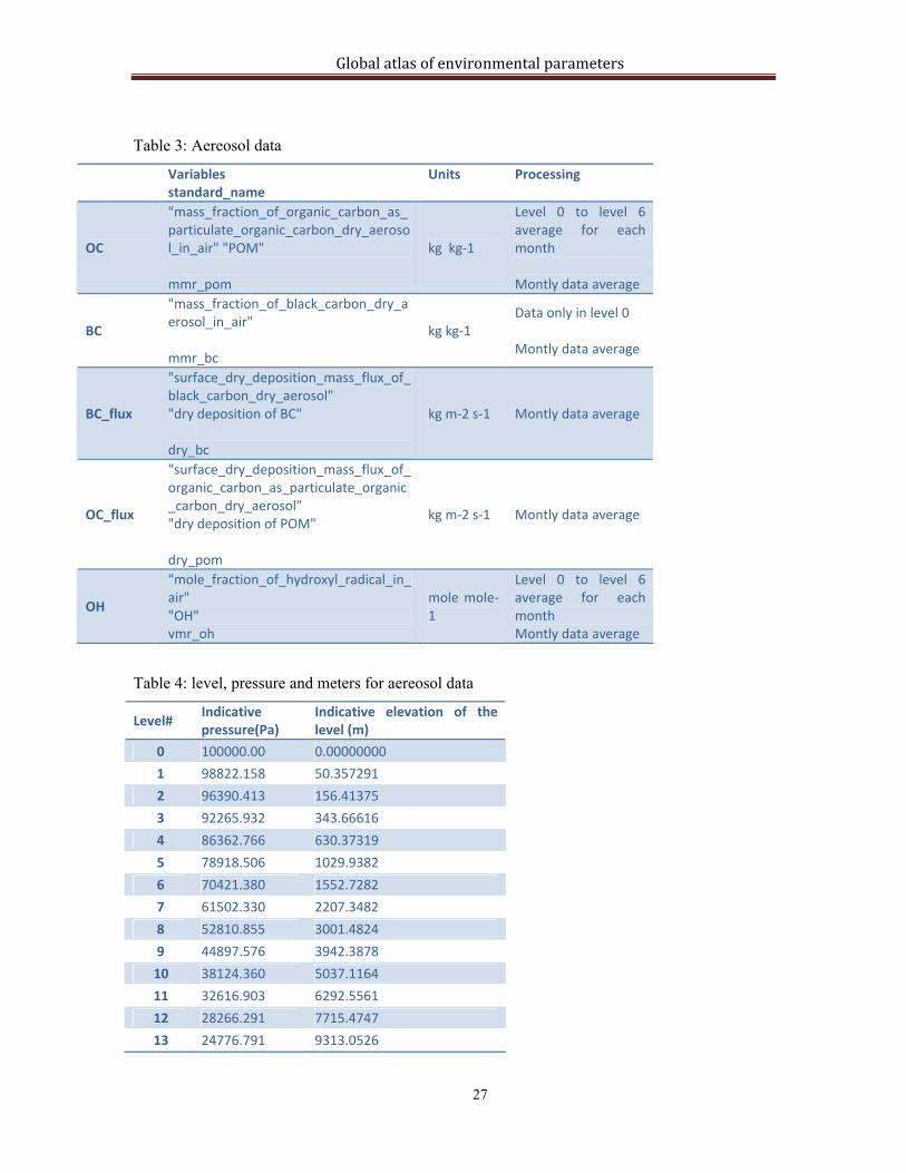
3.6 Aerosol DATA SOURCE Aerosol data were provided by colleagues at the Joint Research Centre - Institute

for Environment and Sustainability, Climate Change Unit,and derive from simulations sun with the TM5 model. The data (summarized in Table 3) were in NetCDF format and were imported an processed as grids of monthly values. Data come referred to months of year 2001 and to a number of vertical atmospheric layers (levels) of which the pressure and indicative elevation is given in Table 4.

FILENAMES

TM5-JRC-cy2-ipcc-v1_SR1_aerosolm_2001.nc TM5-JRC-cy2-ipcc-v1_SR1_depm_2001.nc TM5-JRC-cy2-ipcc-v1_SR1_tracerm_2001.nc

SOURCE CITATION Gregory Carmichael, Frank Dentener, Richard Derwent, Arlene Fiore, Michael

Prather, Michael Schulz, Oliver Wild, Chapter 5: Global and Regional modeling, in Hemispheric Transport of Air pollution 2007, Air pollution studies, 16, United Nations Economic Commission for Europe, ISBN, 1014-4625, Geneva, 2007

Krol, M., Houweling, S., Bregman, B., van den Broek, M., Segers, A., van Velthoven, P., Peters, W., Dentener F., Bergamaschi P., The two-way nested global


26

chemistry-transport zoom model TM5: algorithm and application. Atmos. Chem. Phys. 4, 3975-4018 – 2005.

De Meij, A., M. Krol, F. Dentener, V. E., E. Cuvelier, and P. Thunis, The sensitivity of aerosol in Europe to two different emission inventories and temporal distribution of emissions, Atmospheric Chemistry and Physics, Vol. 6, pp 4287-4309, 25-9-2006.

LINK None ACCESSED 26/10/2009 SPATIAL RESOLUTION 1° x 1° COVERAGE Global TEMPORAL RESOLUTION 2001 PRIMARY DATA FORMAT NetCDF PROCESSING Extracting tables from NETCDF Average of levels 0 to 6 for each month Montly data average STORED IN \\globaldata\Atmosphere\Aereosol\


27

Table 3: Aereosol data

Variables standard_name

Units Processing

OC

"mass_fraction_of_organic_carbon_as_particulate_organic_carbon_dry_aerosol_in_air" "POM" mmr_pom

kg kg‐1

Level 0 to level 6 average for each month Montly data average

BC

"mass_fraction_of_black_carbon_dry_aerosol_in_air" mmr_bc

kg kg‐1 Data only in level 0 Montly data average

BC_flux

"surface_dry_deposition_mass_flux_of_black_carbon_dry_aerosol" "dry deposition of BC" dry_bc

kg m‐2 s‐1 Montly data average

OC_flux

"surface_dry_deposition_mass_flux_of_organic_carbon_as_particulate_organic_carbon_dry_aerosol" "dry deposition of POM" dry_pom

kg m‐2 s‐1 Montly data average

OH

"mole_fraction_of_hydroxyl_radical_in_air" "OH" vmr_oh

mole mole‐1

Level 0 to level 6 average for each month Montly data average

Table 4: level, pressure and meters for aereosol data

Level# Indicative pressure(Pa)

Indicative elevation of the level (m)

0 100000.00 0.00000000

1 98822.158 50.357291

2 96390.413 156.41375

3 92265.932 343.66616

4 86362.766 630.37319

5 78918.506 1029.9382

6 70421.380 1552.7282

7 61502.330 2207.3482

8 52810.855 3001.4824

9 44897.576 3942.3878

10 38124.360 5037.1164

11 32616.903 6292.5561

12 28266.291 7715.4747

13 24776.791 9313.0526


28

14 21748.501 11095.247

15 18777.332 13082.395

16 15563.598 15318.425

17 12099.698 17840.760

18 8765.7189 20685.030

19 6018.0195 23888.502

20 3960.2915 27445.247

21 1680.6403 34730.961

22 713.21808 42016.675

23 298.49579 49420.442

24 95.636963 59095.112

25 0.00000000 Infinity

Figure 14: Mass fraction of organic carbon


29

Figure 15: flux of black carbon dry aerosol

Figure 16: flux of organic carbon dry aerosol


30

NOTES Modeled aerosol concentrations and fluxes werepreferred here to alternatives such

as satellite products from MODIS (http://modis.gsfc.nasa.gov/about/ ; ftp://ladsweb.nascom.nasa.gov/allData/4/MYD08_M3/).

4. Data Catalog: Stream Network

4.1 Networks DATA SOURCE HYDRO1k ORIGINAL DATA DESCRIPTION HYDRO1k is a geographic database developed to provide comprehensive and

consistent global coverage of topographically derived data sets, including streams, drainage basins and ancillary layers derived from the USGS' 30 arc-second digital elevation model of the world (GTOPO30). HYDRO1k provides a suite of geo-referenced data sets, both raster and vector, which will be of value for all users who need to organize, evaluate, or process hydrologic information on a continental scale.

Developed at the U.S. Geological Survey's Center for Earth Resources Observation and Science (EROS), the HYDRO1k project's goal is to provide to users, on a continent by continent basis, hydrologically correct DEMs along with ancillary data sets for use in continental and regional scale modeling and analyses. Detailed descriptions of the processing steps involved in development of the HYDRO1k data sets can be found in the Readme file.

This work was conducted by the U.S. Geological Survey in cooperation with UNEP/GRID Sioux Falls. Additional funding was provided by the Brazilian Water Resources Secretariat and the Food and Agriculture Organization/Inland Water Resources and Aquaculture Service.

Each data set is made up of six raster and two vector layers. Projection and georeferencing information: Africa: Number of rows = 9194 Number of columns = 8736 XY corner coordinates (center of pixel): Lower left: -4368500.000, -5044500.000 Upper left: -4368500.000, 4149500.000 Upper right: 4367500.000, 4149500.000 Lower right: 4367500.000, -5044500.000 Projection used: Lambert Azimuthal Equal Area Units = meters Pixel Size = 1000 meters


31

Radius of Sphere of Influence = 6,370,997 meters Longitude of Origin = 20 00 00E Latitude of Origin = 5 00 00N False Easting = 0.0 False Northing = 0.0 Asia Number of rows = 11882 Number of columns = 9341 XY corner coordinates (edge of pixel): Lower left: -4355500.000, -5438500.000 Upper left: -4355500.000, 6443500.000 Upper right: 4985500.000, 6443500.000 Lower right: 4985500.000, -5438500.000 Projection used: Lambert Azimuthal Equal Area Units = meters Pixel Size = 1000 meters Radius of Sphere of Influence = 6,370,997 meters Longitude of Origin = 100 00 00E Latitude of Origin = 45 00 00N False Easting = 0.0 False Northing = 0.0 Europe Number of rows = 7638 Number of columns = 8319 Lower left: -4091500.000, -4344500.000 Upper left: -4091500.000, 3293500.000 Upper right: 4227500.000, 3293500.000 Lower right: 4227500.000, -4344500.000 Projection used: Lambert Azimuthal Equal Area Units = meters Pixel Size = 1000 meters Radius of Sphere of Influence = 6,370,997 meters Longitude of Origin = 20 00 00E Latitude of Origin = 55 00 00N False Easting = 0.0 False Northing = 0.0 North America Number of rows = 8384 Number of columns = 9102 Lower left: -4462500.000, -3999500.000 Upper left: -4462500.000, 4384500.000


32

Upper right: 4639500.000, 4384500.000 Lower right: 4639500.000, -3999500.000 Projection used: Lambert Azimuthal Equal Area Units = meters Pixel Size = 1000 meters Radius of Sphere of Influence = 6,370,997 meters Longitude of Origin = 100 00 00W Latitude of Origin = 45 00 00N False Easting = 0.0 False Northing = 0.0 South America Number of rows = 9094 Number of columns = 7736 Lower left: -3776500.000, -5258500.000 Upper left: -3776500.000, 3835500.000 Upper right: 3959500.000, 3835500.000 Lower right: 3959500.000, -5258500.000 Projection used: Lambert Azimuthal Equal Area Units = meters Pixel Size = 1000 meters Radius of Sphere of Influence = 6,370,997 meters Longitude of Origin = 60 00 00W Latitude of Origin = 15 00 00S False Easting = 0.0 False Northing = 0.0 SOURCE CITATION USGS EROS Data Center, HYDRO1k Elevation Derivative Database. Sioux

Falls, South Dakota, LP DAAC. LINK http://eros.usgs.gov/#/Find_Data/Products_and_Data_Available/gtopo30/hydro ACCESSED 01/10/2009 SPATIAL RESOLUTION 1km x 1km (0.008333°x0.008333°) Processing - GlobalNet.mdb:

o Vector data (stream network, lakes and basins) for each continent


33

o Mosaic to global extent (except for the Australia dataset); reprojection to wgs84 (filed Shape_area has the polygons’ surface in m2)

Stored in \\globaldata\Stream_Network\StreamNet

4.2 Potential Simulated Topological Networks DATA SOURCE STN-30p ORIGINAL DATA DESCRIPTION The global Simulated Topological Network at 30-minute spatial resolution (STN-

-30p) represents rivers as a set of spatial and tabular data layers derived from a 30-minute flow-direction grid. Simulated Topological Networks are used to represent the linkage of continental land mass and river networks in the Global Hydrologic Archive and Analysis System (GHAAS). STN networks are generated at various resolutions. The 30-minute STN for the world (shown above) is suitable for monthly flow simulations, such as used in the GHAAS Water Transport Model (WTM). Other uses of the STN include the derivation of basin-wide or subbasin characteristics such as stream order, mainstem length and catchment area. Table 5: STN 30p data structure

File Data

g_basin Basin grid with basin attributes

g_celllength Grid cell length [km] grid

g_cumularea Upstream catchment area [km^2] grid

g_distmouth Distance [km] to mouth of river defined as the confluence with equal or higher order stream

g_distocean Distance [km] to the outlet of river basins

g_network Flow‐direction grid

g_order Strahler stream order grid

c_basin Basin polygon coverage with the same basin attributes as the basin grid

c_network Arc/point coverage representing river segments and basin mouths

SOURCE CITATION Simulated Topological Networks (STN-30p) Version 6.01 Link http://www.wsag.unh.edu/Stn-30/stn-30.html ACCESSED


34

25/09/2009 SPATIAL RESOLUTION 30’ cellsize 0.5 PRIMARY DATA FORMAT ARC/INFO coverages and ASCII interchange files STORED IN \\globaldata\Stream_Network\Topo_Net\stn30

4.3 Global Lakes DATA SOURCE World lakes database – See annex A Framework Contract JRC.REF ESP DESIS DI/05712 (LOT 1 B) Link http://www.ilec.or.jp/database/database.html STORED IN \\globaldata\Stream_Network\lakes


35

Figure 17: Stream Networks data type


36

4.4 Average Residence Time (ART) of Pollutants in Inland Surface Water

DATA : Hydro 1K (by Continent) Global Runoff (global) Global Lakes (global) Nighttime Lights of the World (global) SPATIAL RESOLUTION 1km x 1km (0.008333°x 0.008333°) PROCESSING SCHEME The average residence time of a contaminant in a catchment may be defined as:

⎟⎟⎟⎟

⎠

⎞

⎜⎜⎜⎜

⎝

⎛

−=

∑

∑

=

=n

iii

n

ii

ktE

E

kART

1

1

)exp(ln1

Where n is the number of contaminant emissions existing in the catchments, Ei is the intensity (mass discharge) of the i-th emission, and ti is the timeof travel of water from the i-th emission to the catchment outlet, while k is the contaminant decay rate. From the definition, it is clear that ART can be only defined with reference to a given decay rate. However, by assigning a generic value of k the ART provides an idea of the time required for a contaminant to be washed off from a catchment. We computed the ART with reference to a persistent water pollutant with half life of 60 days, according to the procedure detailed below. Emissions are represented through the proxy given by the worldstablelights atnight from satellite images, described below.

The time of travel of water in catchments is computed considering an average water velocity of 0.2 m s-1 in rivers, and a velocity in lakes given by:

L

L

L T

A

V π4

=

where AL is the lake surface area and TL its hydraulic retention time. Examples of steps in the processing chain are shown in


37

Figure 18.

Procedure input output Results description measure units

Compute annual average discharge

Flow direction, annual average runoff (mm)

[Q] The water discharge map computed from runoff in mm using a resolution of 1 km2 =106 m2 is multiplied by the conversion factor 0.0000317=0.001*1000000/86400/365 to have m3s-1.

Compute each lake’s discharge

Zonal statistics (max) of grid [Q] over each lake’s polygon

An attribute of discharge for each lake polygon

M3 s-1

Compute lake volume Lakes.shp, An attribute of volume for each lake polygon

1000000*iii AhmeanV = Vi=Volume in m3 Ai=Surface in km2 hmean i = lake mean deph computed as described in Annex B

Compute average Time of residence in Lakes

Lakes.shp, An attribute of residence time for each lake polygon

T=V/Q/86400 (days)

Compute equivalent flow velocity in lakes

Lakes.shp, An attribute of velocity for each lake polygon

i

i

i T

A

VL π4

=

VLi = speed in m/day for each lake Ai= surface area of each lake Ti= Average Time of residence in Lakes in days Appropriate conversion of units yields m day-1.

Rasterize Lakes.shp, (using previous velocity as attribute)

Lakes.shp, [Vellake], grid

Define a weight representing the average crossing time of in Lakes and the stream network (days per meter)

[Vellake], [mask] (a mask grid representing only rivers above 500 km2 of catchment)

[F_W] ESRI ArcGIS syntax: [F_W]= Con (IsNull([Vellake]), 1 / 0.2 / 86400, 1 / [Vellake]) * [Mask]

Compute time to reach the sea foreach point, through a weighted downstream flowlength using weight F_W

Fdirection, F_W

[tau] Map of the time to reach the sea (days)


38

Procedure input output Results description measure units

Define the product of emission and exp(-kt):

kteEweighLs −∗=_ E=emission T=time to the sea Assuming halflife of 60 days K = 0.011552 (= ln2/60)

[tau], [world_lights]

[Ls_weigh] We assume here world stable lights [world_lights] as a proxy for chemical emissions: [Ls_weigh]=Exp(- 0.011552453 * [tau]) * [world_lights]

Denominator of the logarithm argument in:

⎟⎟⎟⎟

⎠

⎞

⎜⎜⎜⎜

⎝

⎛

−=

∑

∑

=

=n

iii

n

ii

ktE

E

kART

1

1

)exp(ln1

Fdirection, Ls_weigh

[Fl_Acc_W_1] --

Numerator of the logarithm argument in:

⎟⎟⎟⎟

⎠

⎞

⎜⎜⎜⎜

⎝

⎛

−=

∑

∑

=

=n

iii

n

ii

ktE

E

kART

1

1

)exp(ln1

[Fdirection], [world_lights]

[Fl_Acc_W_2] --

Identification of the catchments discharging to the sea

[Fdirection] [Basins] We use an ArcGIS spatial analyst ”basin” operation.

Extraction of the denominator of the logarithm argument by basin

[Fl_Acc_W_1] , [basins]

[zonal1] zonal statistics di [Fl_Acc_W_1] on [basins] (max value)

Extraction of the numerator of the logarithm argument by basin

[Fl_Acc_W_2], [basins]

[zonal2] zonal statistics di [Fl_Acc_W_1] on [basins] (max value)

Compute the logarithm argument

[zonal1], [zonal2]

[TT] zonal1/zonal2

Average Residence Time of Pollutants in Island Surface Water in days

[TT] [LogTT] [LogTT]=Log(1/[TT])/k

STORED IN \\globaldata\Stream_Network\ART


39

Figure 18: main phases of the analysis procedure.


40

Figure 19 : Average residence time of pollutants in surface water


41

5. Data Catalog: Oceans

5.1 Temperature DATA SOURCE World Ocean Atlas 2005 (NOAA) ORIGINAL DATA DESCRIPTION Annual climatological mean of oceanographic temperature at 0-5500 meters (33

levels) SOURCE CITATION Locarnini, R. A., A. V. Mishonov, J. I. Antonov, T. P. Boyer, and H. E. Garcia,

2006. World Ocean Atlas 2005, Volume 1: Temperature. S. Levitus, Ed. NOAA Atlas NESDIS 61, U.S. Government Printing Office, Washington, D.C., 182 pp.

LINK http://www.nodc.noaa.gov/cgi-bin/OC5/SELECT/woaselect.pl?parameter=1 ACCESSED 07/10/2008 SPATIAL RESOLUTION 1°x1° TEMPORAL RESOLUTION 2005 PROCESSING Data are stored in “File GeoDatabase Feature Class” format Average of first 30 meters STORED IN \\globaldata\Ocean\OceanTemp


42

Figure 20: Ocean temperature

5.2 Salinity DATA SOURCE World Ocean Atlas 2005 (NOAA) ORIGINAL DATA DESCRIPTION Annual climatological mean of oceanographic salinity at 0-5500 meters (33

levels) SOURCE CITATION Antonov, J. I., R. A. Locarnini, T. P. Boyer, A. V. Mishonov, and H. E. Garcia,

2006. World Ocean Atlas 2005, Volume 2: Salinity. S. Levitus, Ed. NOAA Atlas NESDIS 62, U.S. Government Printing Office, Washington, D.C., 182 pp.

LINK http://www.nodc.noaa.gov/cgi-bin/OC5/SELECT/woaselect.pl?parameter=2 ACCESSED 07/10/2008 SPATIAL RESOLUTION 1°x 1°


43

TEMPORAL RESOLUTION

PROCESSING Data are stored in “File GeoDatabase Feature Class” format. STORED IN \\globaldata\Ocean\GDB\Ocean.gdb

5.3 Mixed layer depth DATA SOURCE World Ocean Atlas 1994 (NOAA) ORIGINAL DATA DESCRIPTION “The MLD fields available are computed from climatological monthly mean

profiles of potential temperature and potential density based on three different criteria: a temperature change from the ocean surface of 0.5 degree Celsius, a density change from the ocean surface of 0.125 (sigma units), and a variable density change from the ocean surface corresponding to a temperature change of 0.5 degree Celsius. The MLD based on the variable density criterion is designed to account for the large variability of the coefficient of thermal expansion that characterizes seawater.” (documentation from the source - MLD is in meters)

Source citation Monterey, G. and Levitus, S., 1997: Seasonal Variability of Mixed Layer Depth

for the World Ocean. NOAA Atlas NESDIS 14, U.S. Gov. Printing Office, Wash., D.C., 96 pp. 87 figs.

Link http://www.nodc.noaa.gov/OC5/WOA94/mix.html ACCESSED 11/07/2008 SPATIAL RESOLUTION 1°x1° TEMPORAL RESOLUTION Monthly PROCESSING Conversion of original monthly data files to GRID format. STORED IN \\globaldata\Ocean\MLD


44

Figure 21: Mixed Layer Deph

5.4 Chlorophyll DATA SOURCE World Ocean Atlas 2001 (NOAA) ORIGINAL DATA DESCRIPTION 1. Annual mean chlorophyll (µg/l) at the surface. 2. Annual mean chlorophyll (µg/l) at 10 m depth. 3. Annual mean chlorophyll (µg/l) at 20 m depth. 4. Annual mean chlorophyll (µg/l) at 30 m depth. 5. Annual mean chlorophyll (µg/l) at 50 m depth. 6. Annual mean chlorophyll (µg/l) at 75 m depth. 7. Annual mean chlorophyll (µg/l) at 100 m depth. Analyzed fields (an) - One-degree all-data objectively analyzed mean. For all

variables, the annual analyzed field is the average of the twelve monthly fields for each standard level for which monthly fields exist

SOURCE CITATION Conkright, M.E., T.D. O’Brien, C. Stephens, R.A. Locarnini, H.E. Garcia, T.P.

Boyer, J.I. Antonov , 2002: World Ocean Atlas 2001, Volume 6: Chlorophyll. Ed. S. Levitus, NOAA Atlas NESDIS 54, U.S. Government Printing Office, Wash., D.C., 46 pp.


45

LINK http://www.nodc.noaa.gov/OC5/WOA01/1d_woa01.html ACCESSED 11/07/2008 SPATIAL RESOLUTION 1°x1° TEMPORAL RESOLUTION --- PROCESSING Conversion of original files to “File GeoDatabase Raster Dataset” format. Average of first 30 meters STORED IN \\globaldata\Ocean\Chlorophyll


46

Figure 22: Chlorophyll

5.5 Surface velocity DATA SOURCE Mariano Global Surface Velocity analysis ORIGINAL DATA DESCRIPTION The initial input data set is the Maury Ship Drift database from 1900 to 1945.

Each velocity component, u and v, were estimated using the scalar Parameter Matrix Objective Analysis algorithm (PMOA) routine described in Mariano and Brown (1992) after a median filter was applied to the data to remove gross outliers. This data was mapped monthly and has a horizontal resolution of 100 km (Mariano et al, 1995).

Each velocity component, u and v, were estimated using the scalar OA routine described in Mariano and Brown (1992) after a median filter was applied to the data to remove gross outliers. The velocity estimates are poor in the southern ocean due to the lack of data, especially south of 50 S.

SOURCE CITATION Mariano, A.J., E.H. Ryan, B.D. Perkins, S. Smithers. The Mariano Global Surface Velocity analysis 1.0, U.S. Coast Guard Technical Report, CG-D-34-95, 1995.

Mariano, A.J. and O.B. Brown. Efficient objective analysis of dynamically heterogeneous and nonstationary fields via the parameter matrix. Deep-Sea Res., 39 (7/8), 1992, 1255-1271.


47

LINK http://www.rsmas.miami.edu/personal/eryan/mgsva/ ACCESSED 11/07/2008 SPATIAL RESOLUTION 1°x1° UNIT m/s TEMPORAL RESOLUTION 1900-1945 PROCESSING Conversion of original csv files to “File GeoDatabase Feature Class” format. Calculation of velocity:

STORED IN \\globaldata\water\Ocean\Velocity Figure 23: Surface velocity


48

5.6 Water surfaces DATA SOURCE Inputs:

- Lakes: Vector Lakes from the World lake database - Continents shape file from the ESRI digital chart of the world - Mask of ocean/land surface created from the Continents shape file

SPATIAL RESOLUTION 0.25 x 0.25

UNITS % of water surface STORED IN \\globaldata\water\water025_b Figure 24: percentage of water surface


49

6. Data Catalog: Vegetation

6.1 Vegetation Data source Continuous Fields of Vegetation Cover Original data description “The objective of this study was to derive continuous fields of vegetation cover

from multi-temporal Advanced Very High Resolution Radiometer (AVHRR) data using all available bands and derived Normalized Difference Vegetation Index (NDVI). The continuous fields describe sub-pixel proportions of cover for tree, herbaceous, bare ground and water cover types. For tree cover, additional fields describing leaf longevity (evergreen and deciduous) and leaf morphology (broadleaf and needleleaf) were also generated. The modeling of carbon dynamics and climate require knowing tree characteristics such as these. These products were resampled and aggregated to 0.25, 0.5 and 1.0 degree grids for the International Satellite Land Surface Climatology Project (ISLSCP) data initiative II. The data set describes the geographic distributions of three fundamental vegetation characteristics: tree, herbaceous and bare ground cover, plus a water layer. For tree cover, leaf longevity and morphology layers were produced.” ( data set description from the source)

The data sets are provided at three spatial resolutions of 0.25, 0.5 and 1 degrees lat./long. For each spatial resolution there are eight files describing the percentage, from 0 to 100, of the following global continuous fields: Table 6: Vegetation Type

Value Description

1 Bare Cover

2 Herbaceous cover

3 Tree cover

4 Water

5 Deciduous tree cover

6 Evergreen tree cover

7 Needleleaf tree cover

The files for 1) are called bare_percent_xx.asc, where xx is qd, hd, or 1d, denoting a spatial resolution of 1/4, 1/2 or 1degree, respectively. The files for 2) are called herb_percent_xx.asc, with xx as above, and so on for the different continuous fields. Missing data points are listed as -999.

SOURCE CITATION DeFries, R. S., Townshend, J. R. G., and Hansen, M. C., 1999, Continuous fields

of vegetation characteristics at the global scale at 1km resolution, Journal of Geophysical Research, 104, 16 911-16 925.


50

DeFries, R. S., Hansen, M. C., Townshend, J. R. G., Janetos, A. C., and Loveland, T. R., 2000, A new global 1-km dataset of percentage tree cover derived from remote sensing. Global Change Biology, 6, 247-254.

LINK http://islscp2.sesda.com/ISLSCP2_1/html_pages/groups/veg/veg_continuous_fiel

ds_xdeg.html ACCESSED 16/07/2008 SPATIAL RESOLUTION 1°x1°, 0.5°x0.5°, 0.25°x0.25° TEMPORAL RESOLUTION 1992-1993 PROCESSING Import of 0.25°x0.25° files into “File GeoDatabase Raster Dataset” format. STORED IN \\globaldata\Others\GDB\Others.gdb \\globaldata\Others\Vegetation (grid format)


51

Figure 25: percentage of deciduous tree cover

Figure 26: evergreen tree cover


52

7. Data Catalog: Antrophic Factors

7.1 World stable lights DATA SOURCE world_stable_lights - World stable lights percent frequency file. ORIGINAL DATA DESCRIPTION “The Defense Meteorological Satellite Program (DMSP) Operational Linescan

System (OLS) has a unique low-light imaging capability developed for the detection of clouds using moonlight. In addition to moonlit clouds, the OLS also detects lights from human settlements, fires, gas flares, heavily lit fishing boats, lightning and the aurora. By analyzing the location, frequency, and appearance of lights observed in an image times series, it is possible to distinguish four primary types of lights present at the earth's surface: human settlements, fires, gas flares, and fishing boats. We have produced a global map of the four types of light sources as observed during a 6-month period in 1994 - 1995.” (documentation from the source)

This file is the cities and flares combined. SOURCE CITATION --- LINK http://www.ngdc.noaa.gov/dmsp/download_Night_time_lights_94-95.html ACCESSED 16/10/2008 SPATIAL RESOLUTION 30”x30”, 1”x1” TEMPORAL RESOLUTION 1994-1995 PROCESSING Import of original tiff files into “File GeoDatabase Raster Dataset” format. STORED IN \\globaldata\Others\GDB\Others.gdb \\globaldata\Others\W_lights (GRID format)


53

Figure 27: Percent frequency of World Stable Lights


54

7.2 Population counts, population density DATA SOURCE Gridded Population of the World Version 3 (GPWv3) ORIGINAL DATA DESCRIPTION This archive contains population counts and population densities, both UN-

adjusted and unadjusted, in ArcInfo GRID format. The raster data are at 2.5 arc-minutes resolution and contain the following data:

p00g population counts in 2000, unadjusted p00ag population counts in 2000, adjusted to match UN totals ds00g population densities in 2000, unadjusted, persons per square km ds00ag population densities in 2000, adjusted to match UN totals, persons per

square km The data are stored in geographic coordinates of decimal degrees based on the

World Geodetic System spheroid of 1984 (WGS84). SOURCE CITATION Center for International Earth Science Information Network (CIESIN), Columbia

University; and Centro Internacional de Agricultura Tropical (CIAT). 2005. Gridded Population of the World Version 3 (GPWv3): Population Grids. Palisades, NY: Socioeconomic Data and Applications Center (SEDAC), Columbia University. Available at http://sedac.ciesin.columbia.edu/gpw.

LINK http://sedac.ciesin.columbia.edu/gpw/index.jsp ACCESSED 27/11/2008 SPATIAL RESOLUTION 2.5’x2.5’ TEMPORAL RESOLUTION 2000 PROCESSING Import of files into “File GeoDatabase Raster Dataset” format. STORED IN \\globaldata\Others\GDB\Others.gdb


55

Figure 28: population density


56

7.1 Impervious Surface Area DATA SOURCE Global Distribution and Density of Constructed Impervious Surfaces (NOAA-

NESDIS-NGDC-DMSP) ORIGINAL DATA DESCRIPTION “We present the first global inventory of the spatial distribution and density of

constructed impervious surface area (ISA). Examples of ISA include roads, parking lots, buildings, driveways, sidewalks and other manmade surfaces. While high spatial resolution is required to observe these features, the product we made is at one km2 resolution and is based on two coarse resolution indicators of ISA. Inputs into the product include the brightness of satellite observed nighttime lights and population count. The reference data used in the calibration were derived from 30 meter resolution ISA estimates of the USA from the U.S. Geological Survey. Nominally the product is for the years 2000-01 since both the nighttime lights and reference data are from those two years. We found that 1.05% of the United States land area is impervious surface (83,337 km2 ) and 0.43% of the world's land surface (579,703 km2 ) is constructed impervious surface. China has more ISA than any other country (87,182 km2 ), but has only 67 m2 of ISA per person, compared to 297 m2 per person in the USA. Hydrologic and environmental impacts of ISA begin to be exhibited when the density of ISA reaches 10% of the land surface. An examination of the areas with 10% or more ISA in watersheds finds that with the exception of Europe, the majority of watershed areas have less than 0.4% of their area at or above the 10% ISA threshold. The authors believe the next step for improving the product is to include reference ISA data from many more areas around the world.” (documentation from the source)

SOURCE CITATION Elvidge, C.D., Tuttle, B.T., Sutton, P.C., Baugh, K.E., Howard, A.T., Milesi, C.,

Bhaduri, B.L., and Nemani, R. 2007. Global distribution and density of constructed impervious surfaces. Sensors 7: 1962-1979.

LINK http://www.ngdc.noaa.gov/dmsp/download_global_isa.html ACCESSED 14/10/2008 SPATIAL RESOLUTION 30” (~1km) TEMPORAL RESOLUTION 2000-2001 PROCESSING


57

Import of original geotiff file into “File GeoDatabase Raster Dataset” format. STORED IN \\globaldata\AntrophicF\Impervious

Figure 29: percentage of impervious surface


58

Value data source temporal res spatial res

FAO soil map OC content Bulk density

www.isric.org // 5’

Global soil texture and derived water‐holding capacities (webb et al.)

Texture daac.ornl.gov //

Soil Moisture Storage Capacity (mm/m) [Maximum available soil moisture]

Soil Moisture www.fao.org // 5’

UNH‐GRDC Global Composite Runoff Fields Runoff grdc.bafg.de // 0.5°

Soil

Sediment Removal Rate for basins Sediments Yeld JRC original model //

Surface, Boundary layer height , 40 years reanalysis

ABL mixing height http://data‐portal.ecmwf.int/data/d/era40_mnth/

1957/09‐2002/08

2.5°

mnth, Surface, 2 metre temperature, 40 years reanalysis

Temperature http://data‐portal.ecmwf.int/data/d/era40_mnth/

1957/09‐2002/08

2.5°

Surface, mnth, 10 metre U wind and V wind component , 40 years reanalysis

Wind Speed http://data‐portal.ecmwf.int/data/d/era40_mnth/

1957/09‐2002/08

2.5°

Total Precipitation, 40 years reanalysis Total Precipitation http://data‐portal.ecmwf.int/data/d/era40_mnth/

1957/09‐2002/08

2.5°

Snow Fall, 40 years reanalysis Snow Fall http://data‐portal.ecmwf.int/data/d/era40_mnth/

1957/09‐2002/08

2.5°

OC BC_flux OC_flux

Atm

osph

ere

Aerosol Indexes

OH

JRC // 1°

World Ocean Atlas 2005 (WOA05) temperature, salinity www.nodc.noaa.gov // 1°

World Ocean Atlas 1994 (WOA94) mixed layer depth www.nodc.noaa.gov // 1°

World Ocean Atlas 2001(WOA01) chlorophyll www.nodc.noaa.gov // 1° Ocean

The Mariano Global Surface Velocity Analysis 1.0 (MGSVA)

surface velocity www.rsmas.miami.edu yearly 1°

Conclusions and recommendations

59

Networks Hydro 1k edc.usgs.gov // 30‘’ (~1km)

Potential Simulated Topological Network

stn30 http://www.wsag.unh.edu/Stn‐30/stn‐30.html

// 30’ cellsize 0.5

Global Lakes wwf

Stream

Network

Average Residence Time of Pollutants in Island Surface Water

Hydro 1k, runoff, global lakes, lights at night

Derived model // 30‘’ (~1km)

Continuous Fields of Vegetation Cover vegetation islscp2.sesda.com 1992‐1993 1°, 0.5°, 0.25°

FASIR NDVI Monthly vegetation islscp2.sesda.com 1982‐1998 1°, 0.5°, 0.25°

World stable lights lights at night www.ngdc.noaa.gov

1994‐1995 30”, 1”

Global Population of the World population counts, population density

http://sedac.ciesin.columbia.edu

2000 1°, 2.5’

Other

Impervious Surface Area ISA http://www.ngdc.noaa.gov/dmsp/download_global_isa.html

2000‐2001 30‘’ (~1km)

Softwares

60

8. Softwares 8.1.1 Arcgis 9.x

Proprietary software http://www.esri.com/ Principal platform for data preparation, visualization, analysis, cartography ArcHydro extension

8.1.2 Panoply Netcdf viewer http://www.giss.nasa.gov/tools/panoply/

8.1.3 NCO operators The netCDF Operators, or NCO, are a suite of programs known as operators. Each

operator is a standalone, command line program which is executed at the UNIX shell-level. The operators are primarily designed to aid manipulation and analysis of gridded scientific data.

http://nco.sourceforge.net/

8.1.4 Ilwis 3.3 The Integrated Land and Water Information System (ILWIS) is a PC-based GIS &

Remote Sensing software, developed by ITC up to its last release (version 3.3) in 2005. ILWIS comprises a complete package of image processing, spatial analysis and digital mapping.

http://www.itc.nl/ilwis/downloads/ilwis33.asp

8.1.5 HDF http://gis-lab.info/programs-eng.html#libraries

Softwares

61

9. Annex A - Data mining from the online World Lake Database

(http://www.ilec.or.jp/database/database.html) The scraping of data is performed using the software Web-Harvest (http://web-

harvest.sourceforge.net/): “Web-Harvest is Open Source Web Data Extraction tool written in Java. It

offers a way to collect desired Web pages and extract useful data from them. In order to do that, it leverages well established techniques and technologies for text/xml manipulation such as XSLT, XQuery and Regular Expressions.”

The following script has been used to extract data from the ILEC web site:

<?xml version="1.0" encoding="UTF-8"?> <config charset="ISO-8859-1">  <var-def name="startUrl">http://www.ilec.or.jp/database/index/idx-

lakes.html</var-def> <file action="write" path="D:/LakesDB/webharvest/output_lakes.xml"

charset="UTF-8"> <template> <![CDATA[ <lakes> ]]> </template> <loop item="lakeUrl" index="i">  <list> <xpath expression="//div[@id='main']//a[starts-with(@href,

'../')]/@href"> <html-to-xml> <http url="${startUrl}"/> </html-to-xml> </xpath> </list>  <body> <xquery> <xq-param name="doc"> <html-to-xml> <http url="${sys.fullUrl(startUrl, lakeUrl)}"/> </html-to-xml> </xq-param> <xq-expression><![CDATA[ declare variable $doc as node() external; let $sitename :=

data($doc//div[@id='main']/table[1]/tbody/tr[1]/td[1]) let $lakename :=

data($doc//div[@id='main']/table[1]/tbody/tr[2]/td[1]) let $state :=

data($doc//div[@id='main']/table[1]/tbody/tr[3]/td[1]) let $country :=

data($doc//div[@id='main']/table[1]/tbody/tr[4]/td[1]) let $latitude :=

data($doc//div[@id='main']/table[1]/tbody/tr[5]/td[1]) let $longitude :=

data($doc//div[@id='main']/table[1]/tbody/tr[6]/td[1]) let $altitude :=

data($doc//div[@id='main']/table[1]/tbody/tr[7]/td[1]) let $surfacearea :=

Softwares

62

data($doc//div[@id='main']/table[2]/tbody/tr[1]/td[1]) let $volume :=

data($doc//div[@id='main']/table[2]/tbody/tr[1]/td[2]) let $maxdepth :=

data($doc//div[@id='main']/table[2]/tbody/tr[2]/td[1]) let $meandepth :=

data($doc//div[@id='main']/table[2]/tbody/tr[2]/td[2]) let $waterlevelcontrol :=

data($doc//div[@id='main']/table[2]/tbody/tr[3]/td[1]) let $waterlevelfluctuation :=

data($doc//div[@id='main']/table[2]/tbody/tr[3]/td[2]) let $lengthofshoreline :=

data($doc//div[@id='main']/table[2]/tbody/tr[4]/td[1]) let $residencetime :=

data($doc//div[@id='main']/table[2]/tbody/tr[4]/td[2]) let $catchmentarea :=

data($doc//div[@id='main']/table[2]/tbody/tr[5]/td[1]) let $hoursofbrightsunshine :=

data($doc//div[@id='main']/table[2]/tbody/tr[5]/td[2]) let $solarradiation :=

data($doc//div[@id='main']/table[2]/tbody/tr[6]/td[1]) let $freezingperiod :=

data($doc//div[@id='main']/table[2]/tbody/tr[6]/td[2]) let $mixingtype :=

data($doc//div[@id='main']/table[2]/tbody/tr[7]/td[1]) let $annualfishcatch :=

data($doc//div[@id='main']/table[2]/tbody/tr[7]/td[2]) let $totalnloading :=

data($doc//div[@id='main']/table[2]/tbody/tr[8]/td[1]) let $totalploading :=

data($doc//div[@id='main']/table[2]/tbody/tr[8]/td[2]) let $population :=

data($doc//div[@id='main']/table[2]/tbody/tr[9]/td[1]) let $popdensofcatchmentarea :=

data($doc//div[@id='main']/table[2]/tbody/tr[9]/td[2]) let $domesticwaterusage :=

data($doc//div[@id='main']/table[3]/tbody/tr[1]/td[1]) let $irrigationwaterusage :=

data($doc//div[@id='main']/table[3]/tbody/tr[1]/td[2]) let $industrialwaterusage :=

data($doc//div[@id='main']/table[3]/tbody/tr[2]/td[1]) let $powergenerationusage :=

data($doc//div[@id='main']/table[3]/tbody/tr[2]/td[2]) let $lunaturallandscape :=

data($doc//div[@id='main']/table[4]/tbody/tr[1]/td[1]) let $luagriculturalland :=

data($doc//div[@id='main']/table[4]/tbody/tr[1]/td[2]) let $luothers :=

data($doc//div[@id='main']/table[4]/tbody/tr[1]/td[3]) let $siltation :=

data($doc//div[@id='main']/table[5]/tbody/tr[1]/td[1]) let $toxiccontamination :=

data($doc//div[@id='main']/table[5]/tbody/tr[1]/td[2]) let $eutrophication :=

data($doc//div[@id='main']/table[5]/tbody/tr[2]/td[1]) let $acidification :=

data($doc//div[@id='main']/table[5]/tbody/tr[2]/td[2]) return <lake> <site_name>{data($sitename)}</site_name> <lake_name>{data($lakename)}</lake_name> <state>{data($state)}</state> <country>{data($country)}</country> <latitude>{data($latitude)}</latitude> <longitude>{data($longitude)}</longitude> <altitude>{data($altitude)}</altitude> <surface_area>{data($surfacearea)}</surface_area> <volume>{data($volume)}</volume> <maximum_depth>{data($maxdepth)}</maximum_depth> <mean_depth>{data($meandepth)}</mean_depth>

Softwares

63

<water_level_control>{data($waterlevelcontrol)}</water_level_control> <water_level_fluctuation>{data($waterlevelfluctuation)}</water_level_fluctuation> <length_of_shoreline>{data($lengthofshoreline)}</length_of_shoreline> <residence_time>{data($residencetime)}</residence_time> <catchment_area>{data($catchmentarea)}</catchment_area> <hours_of_bright_sunshine>{data($hoursofbrightsunshine)}</hours_of_bright_sunshine

> <solar_radiation>{data($solarradiation)}</solar_radiation> <freezing_period>{data($freezingperiod)}</freezing_period> <mixing_type>{data($mixingtype)}</mixing_type> <annual_fish_catch>{data($annualfishcatch)}</annual_fish_catch> <total_n_loading>{data($totalnloading)}</total_n_loading> <total_p_loading>{data($totalploading)}</total_p_loading> <population>{data($population)}</population> <population_density_of_catchment_area>{data($popdensofcatchmentarea)}</population_

density_of_catchment_area> <domestic_water_usage>{data($domesticwaterusage)}</domestic_water_usage> <irrigation_water_usage>{data($irrigationwaterusage)}</irrigation_water_usage> <industrial_water_usage>{data($industrialwaterusage)}</industrial_water_usage> <power_generation_usage>{data($powergenerationusage)}</power_generation_usage> <land_use_natural_landscape>{data($lunaturallandscape)}</land_use_natural_landscap

e> <land_use_agricultural_land>{data($luagriculturalland)}</land_use_agricultural_lan

d> <land_use_others>{data($luothers)}</land_use_others> <siltation>{data($siltation)}</siltation> <toxic_contamination>{data($toxiccontamination)}</toxic_contamination> <eutrophication>{data($eutrophication)}</eutrophication> <acidification>{data($acidification)}</acidification> </lake> ]]></xq-expression> </xquery> </body> </loop> <![CDATA[ </lakes> ]]> </file> </config>

(North America lake tabs are encoded differently; therefore a slightly modified code has been used to extract those data)

The output file, in XML format, looks like:

<lakes> <lake> <site_name>AFR-11</site_name> <lake_name>Lake Albert</lake_name> <state>Haut-Zaire, Zaire; and Western, Uganda</state> <country>Zaire and Uganda</country> <latitude>1:4N</latitude> <longitude>30:5E</longitude> <altitude>615</altitude> <surface_area>5,300,000,000</surface_area> <volume>280,000,000,000</volume> <maximum_depth>58</maximum_depth> <mean_depth>25</mean_depth> <water_level_control>Unregulated</water_level_control> <water_level_fluctuation>0.45</water_level_fluctuation> <length_of_shoreline>-</length_of_shoreline> <residence_time>-</residence_time> <catchment_area>-</catchment_area> <hours_of_bright_sunshine>2,190</hours_of_bright_sunshine> <solar_radiation>-</solar_radiation> <freezing_period>None</freezing_period> <mixing_type>Monomictic</mixing_type> <annual_fish_catch>10,000</annual_fish_catch> <total_n_loading>-</total_n_loading>

Softwares

64

<total_p_loading>-</total_p_loading> <population>-</population> <population_density_of_catchment_area>-

</population_density_of_catchment_area> <domestic_water_usage>-</domestic_water_usage> <irrigation_water_usage>-</irrigation_water_usage> <industrial_water_usage>-</industrial_water_usage> <power_generation_usage>-</power_generation_usage> <land_use_natural_landscape>-</land_use_natural_landscape> <land_use_agricultural_land>-</land_use_agricultural_land> <land_use_others>-</land_use_others> <siltation>-</siltation> <toxic_contamination>-</toxic_contamination> <eutrophication>Serious</eutrophication> <acidification>-</acidification> </lake> <lake> <site_name>AFR-19</site_name> <lake_name>Aswan High Dam Reservoir</lake_name> <state>Aswan, Egypt; and Northern, Sudan</state> <country>Egypt and Sudan</country> <latitude>22:1N</latitude> <longitude>31:4E</longitude> <altitude>183</altitude> <surface_area>6,000,000,000</surface_area> <volume>162,000,000,000</volume> <maximum_depth>110</maximum_depth> <mean_depth>70</mean_depth> <water_level_control>Regulated</water_level_control> <water_level_fluctuation>25</water_level_fluctuation> <length_of_shoreline>9,000,000</length_of_shoreline> <residence_time>-</residence_time> <catchment_area>2,849,000,000,000</catchment_area> <hours_of_bright_sunshine>3,866.6</hours_of_bright_sunshine> <solar_radiation>-</solar_radiation> <freezing_period>None</freezing_period> <mixing_type>Monomictic</mixing_type> <annual_fish_catch>18,000</annual_fish_catch> <total_n_loading>-</total_n_loading> <total_p_loading>-</total_p_loading> <population>-</population> <population_density_of_catchment_area>-

</population_density_of_catchment_area> <domestic_water_usage>-</domestic_water_usage> <irrigation_water_usage>-</irrigation_water_usage> <industrial_water_usage>-</industrial_water_usage> <power_generation_usage>-</power_generation_usage> <land_use_natural_landscape>-</land_use_natural_landscape> <land_use_agricultural_land>-</land_use_agricultural_land> <land_use_others>-</land_use_others> <siltation>Serious</siltation> <toxic_contamination>-</toxic_contamination> <eutrophication>-</eutrophication> <acidification>None</acidification> </lake> ... ... ... ... </lakes>

The xml file is then imported into Excel for further processing. In particular,

latitude and longitude values must be formatted into standard Degree Minutes Seconds format DDD°MM’SS”d (where d=N or S or W or E). For instance:

14:4N, 30:5E 14°40’N, 30°50’E

Softwares

65

Afterward the Excel table is imported as .dbf table into ArcGIS, where latitude and longitude values are converted to Decimal Degrees (creation of 2 new fields, lat_deg and lon_deg) with the field calculator, using the following script:

'========================= 'field_DMS2DD.cal 'Author: Ianko Tchoukanski 'http://www.ian-ko.com '========================= … Data are now ready to be imported into ArcGIS as a geographic layer. This step is

achieved using the “Add XY data” tool. The result of this operation is then exported as point shapefile (ILEC_lakes) as shown in Figure 30.

Figure 30: spatial distribution of the world lakes from the ILEC database

66

9.1 Mean depth Values for the mean depth ( h ) parameter are missing for all lakes in the North America

(NAM) section, therefore it has been calculated by dividing the lake's volume by its surface area. Mean depth values were retrieved from wikipedia for five other lakes missing mean depth

values. Note that values of h for lakes Kyoga and Hazen have the same values of their max depth and thus are probably incorrect. However, for the purposes of the analysis they were considered to be representative as well.

Table 7 : Source: wikipedia.

Name Mean deph (m)

Lake Kyoga 5.7

Danau Toba (Lake Toba) 212

Lake Okeechobee 2.7

Hazen Lake 280

Lake Nahuel Huapi 157

9.2 GLWD integration The point shapefile is next spatially joined with the global lakes and wetlands database GLWD. The point shapefile is somehow inaccurate in regard to latitude and longitude values, because

the values in the original ILEC database are rounded to 1 minute of degree. Because of this limitation, the spatial join with the global lakes and wetlands database GLWD

produces inaccurate results. Therefore the next step of the procedure consists in the manual editing of the point shapefile to

correct the points falling outside the GLWD polygons. As a final point, latitude and longitude values are re-calculated for all lakes.

67

10. Annex B - Estimation of parameters to predict mean lake depth on a global scale.

10.1.1 Conversion of Hydro1k dataset to GRID format HYDRO1k, developed at the U.S. Geological Survey's (USGS) EROS Data Center, is a

geographic database providing comprehensive and consistent global coverage of topographically derived data sets. Developed from the USGS' 30 arc-second digital elevation model (DEM) of the world (GTOPO30), HYDRO1k provides a standard suite of geo-referenced data sets (at a resolution of 1 km) developed on a continent by continent basis, for all landmasses of the globe with the exception of Antarctica and Greenland. The HYDRO1k package provides, for each continent, a suite of six raster and two vector data sets. These data sets cover many of the common derivative products used in hydrologic analysis. The raster data sets are the hydrologically correct DEM, derived flow directions, flow accumulations, slope, aspect, and a compound topographic (wetness) index. The derived streamlines and basins are distributed as vector data sets.

(Hydro1k Documentation) The following procedure prepares the Hydro1k files (dem) for further use in ArcGIS.

Load Hydro1k dem file into ArcGIS (xx_dem.bil) Export data to GRID format (xx_dem) Set Spatial Analyst options Extent and Cell Size both to “Same as Layer xx_dem” Open the Raster Calculator tool Evaluate the following expression:

CON([xx_dem] >= 32768, [xx_dem] - 65536, [xx_dem) (cell values greater than or equal to 32768 are an artifact of the original conversion,

where the 16th bit was interpreted as an integer rather than a negative sign) Evaluate the following expression:

SETNULL([Calculation] == -9999, [Calculation]) (This statement converts all raster values equal to -9999 (oceans) to ‘no data’)

Make permanent Calculation2 (i.e. as xx_dem_grid) Apply the correct spatial reference Reproject dataset to wgs84

10.1.2 Calculation of parameters Statistics have been calculated in ArcGIS for the following parameters, ΔZmax, slope, CTI and

TPI indexes and curvature, in order to find out significant correlations with the measured mean depths extracted from the ILEC database.

Only natural lakes have been selected for the analysis, thus all lakes with dams have been removed from the data sample.

10.1.2.1 Landscape roughness index ΔZmax ΔZmax is the local elevation range, calculated on the Hydro1k dem using a kernel value of

10km*10km (Pistocchi and Pennington, 2006). Procedure:

Open the Neighborhood Statistics tool and execute it with the following parameters: Statistic type: range Neighborhood: rectangle Height: 10 km Width: 10 km

Save the output raster as xx_dem_dz

68

Evaluate the following expression: merge([af_dem_dz], [as_dem_dz], [au_dem_dz], [eu_dem_dz], [na_dem_dz],

[sa_dem_dz]) Make permanent “Calculation” as global_dem_dz Execute Zonal statistics of global_dem_dz with ILEC db lake polygons Join statistics with lakes layer and export the table to Excel for further analysis

10.1.2.2 Slope The Hydro1k slope dataset describes the maximum change in the elevations between each cell

and its eight neighbors (Hydro1k Documentation). The zonal statistic tool has been used to calculate statistics for different values of buffer rings

around 178 lakes of the ILEC database (buffer size of 1, 2, 5, 10, 15, 18, 20, 25, 30 and 50 km). Procedure:

Create different size of rings around lakes (using buffer and erase tools) Create global_slope grid using the following expression:

merge([af_slope], [as_slope], [au_slope], [eu_slope], [na_slope], [sa_slope]) Execute Zonal statistics of global_slope with ring polygons Join statistics with lakes layer and export the table to Excel for further analysis

10.1.2.3 Wetness Index (CTI) The Compound Topographic Index (CTI), commonly referred to as the Wetness Index, is a

function of the upstream contributing area and the slope of the landscape. The CTI is calculated using the flow accumulation (FA) layer along with the slope as CTI = ln ( FA / tan (slope) ) (Hydro1k Documentation).

Procedure: Create global_cti grid using the following expression:

merge([af_cti], [as_cti], [au_cti], [eu_cti], [na_cti], [sa_cti]) Execute Zonal statistics of global_cti with lake polygons Join statistics with lakes layer and export the table to Excel for further analysis

10.1.2.4 Topographic Position Index (TPI) The Topographic Position Index (TPI) is the difference between a cell elevation value and the

average elevation of the neighborhood around that cell. Positive values mean the cell is higher than its surroundings while negative values mean it is lower (Weiss, 2001).

Procedure: Create af,as,au,eu,na,sa TPI grids using the CorridorDesigner tool (www.corridordesign.org) Create global_tpi grid using the following expression:

merge([af_tpi], [as_tpi], [au_tpi], [eu_tpi], [na_tpi], [sa_tpi]) Execute Zonal statistics of global_tpi with lake polygons Join statistics with lakes layer and export the table to Excel for further analysis

10.1.3 Analysis of parameters The analysis of parameters potentially explaining mean lake depth was conducted as explained

below. Only lakes having a natural morphology, i.e. for which no existing dam was reported, were considered.

10.1.3.1 Landscape roughness index ΔZmax Evaluating R2 for each statistic, the SUM of ΔZmax shows the second-best correlation with the

measured mean depth (after RANGE); however, the distribution of errors for SUM is more even than

69

for RANGE, where a larger scatter of the data appears at lower depths. Therefore, the SUM has been retained for further analyses (Figure 31).

Figure 31 – above: R2 values for different zonal statistics of the landscape roughness parameter; below:

scatter plot for the chosen predictor (sum)

10.1.3.2 Slope The best correlation with measured mean heights is found for the 18 km distance ring

(R2=0.592), using the SUM statistic.

dz sum

y = 1832.1x + 3424.6R2 = 0.3595

1.00

10.00

100.00

1000.00

10000.00

100000.00

1000000.00

10000000.00

0.10 1.00 10.00 100.00 1000.00

SUMLinear (SUM)

0

0.1

0.2

0.3

0.4

0.5

0.6

0.7

0.8

0.9

1

MIN MAX RANGE MEAN STD SUM VARIETY MAJORITY MINORITY MEDIAN

R2

70

0

0.1

0.2

0.3

0.4

0.5

0.6

0.7

0 1 2 5 10 15 18 20 25 30 50

buffer size (km)

R2

slope (18 km buffer)

R2 = 0.592

1.00

10.00

100.00

1000.00

10000.00

100000.00

1000000.00

10000000.00

0.10 1.00 10.00 100.00 1000.00

SUMLinear (SUM)

Figure 32 - above: R2 values for different buffer distances; below: scatter plot for the chosen predictor

(18 km buffer)

10.1.3.3 Wetness Index (CTI) CTI index shows no relevant correlation with measured mean depth. Results are not shown

here for simplicity.

10.1.3.4 Topographic Position Index (TPI) The best correlation with measured mean heights is found using the RANGE statistic (R2=0.3):

71

0

0.1

0.2

0.3

0.4

0.5

0.6

0.7

0.8

0.9

1

MIN MAX RANGE MEAN STD SUM

TPI

y = 1.3862x + 156.71R2 = 0.3014

1.00000000000

10.00000000000

100.00000000000

1000.00000000000

0.10 1.00 10.00 100.00 1000.00

RANGELinear (RANGE)

Figure 33 - above: R2 values for different zonal statistics of the TPI; below: scatter plot for the chosen

predictor (range)

10.1.3.5 Surface Area /Catchment area ratio (“Area” parameter) The ratio between lake surface area and its catchment area has a correlation with the measured

mean depth of R2=0.09:

72

Surface area / catchment area

y = 0.0007x + 0.1047R2 = 0.0886

0.001

0.01

0.1

1

10

0.10 1.00 10.00 100.00 1000.00

surf_A/catch_ALinear (surf_A/catch_A)

Figure 34 – scatter plot of “area” and mean lake depth.

10.1.4 Regression analysis Values of R2 for each investigated parameter are summarized hereafter:

dz (SUM) slope 18km

(SUM) TPI

(RANGE) surf_A/catch_A CTI

(MIN) 0.505354324 0.633504556 0.282630341 0.088565494 negligible

Table 8

0

0.1

0.2

0.3

0.4

0.5

0.6

0.7

0.8

0.9

1

dz (SUM) slope 18km (SUM) TPI (RANGE) surf_A/catch_A CTI (MIN)

Figure 35

Slope and dZ seems to be correlated together, therefore dZ is discarded as the slope parameter shows a better R2 value:

73

slope (SUM) dz

(SUM) slope

(SUM) 1 dz

(SUM) 0.943943768 1

Table 9

CTI parameter is discarded too, as its R2 value is not significant enough. The model is subsequently tested with slope, TPI and surf_A/catch_A parameters for R2, both with

normal and logarithmic values.

10.1.4.1 Slope regression analysis

10.1.4.1.1 Normal Regression Statistics

Multiple R 0.795929994 R Square 0.633504556 Adjusted R

Square 0.631213959 Standard Error 42.79118334 Observations 162

Coefficients Intercept 10.13893941 slope 18km

(SUM) 5.65646E-05

Table 10

slope

R2 = 0.6335

1.00000

10.00000

100.00000

1000.00000

0.10 1.00 10.00 100.00 1000.00

Modeled mdLinear (Modeled md)

Figure 36

10.1.4.1.2 Logarithmic Regression Statistics

Multiple R 0.625410478

74

R Square 0.391138266 Adjusted R


Coefficients Intercept -2.260368352 slope 18km

(SUM) 0.643134427

Table 11

slope

R2 = 0.3911

0.0

0.5

1.0

1.5

2.0

2.5

-0.5 0.0 0.5 1.0 1.5 2.0 2.5 3.0

modeled mdLinear (modeled md)

Figure 37

10.1.4.2 Slope-area regression analysis

10.1.4.2.1 Linear Regression Statistics



Coefficients Intercept 2.507264226 slope 18km

(SUM) 5.45269E-05 surf_A/catch_A 64.94439138

Table 12

75

slope-area

R2 = 0.6585

1.00000

10.00000

100.00000

1000.00000

0.10 1.00 10.00 100.00 1000.00

Modeled mdLinear (Modeled md)Linear (Modeled md)

Figure 38

10.1.4.2.2 Logarithmic Regression Statistics




(SUM) 0.647733323 surf_A/catch_A 0.169440781

Table 13

76

slope-area

R2 = 0.4124

0

0.5

1

1.5

2

2.5

-0.5 0.0 0.5 1.0 1.5 2.0 2.5 3.0


Figure 39

10.1.4.3 Slope-TPI-area regression analysis

10.1.4.3.1 Linear Regression Statistics




(SUM) 5.0213E-05 TPI (RANGE) 0.038209166 surf_A/catch_A 68.51706482

Table 14

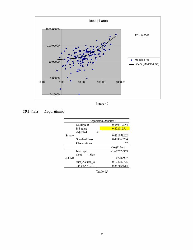
77

slope-tpi-area

R2 = 0.6643

0.10000

1.00000

10.00000

100.00000

1000.00000

0.10 1.00 10.00 100.00 1000.00

Modeled mdLinear (Modeled md)

Figure 40

10.1.4.3.2 Logarithmic

Regression Statistics Multiple R 0.650319584 R Square 0.422915561 Adjusted R



(SUM) 0.47287997 surf_A/catch_A 0.174982795 TPI (RANGE) 0.247166614

Table 15

78

slope-tpi-area

R2 = 0.4229

0

0.5

1

1.5

2

2.5

-0.5 0.0 0.5 1.0 1.5 2.0 2.5 3.0


Figure 41

10.1.5 Conclusions The model based on slope-TPI-area parameters shows the best correlation R2 for both

logarithmic and normal regression analysis. Logarithmic models show worse performance than linear models.

Slope Slope-area Slope-TPI-area

Normal 0.633 0.658 0.664 Logarithmic 0.391 0.412 0.423

Table 16

10.2 Application of the Slope-area model on global scale. The model equation selected for analysis was the one dependent on slope and area, as the

improvement given by introducing TPI was deemed negligible. The equation for mean lake depth is: y = 2.5072642258973 + 0.0000545269266431377x1 + 64.9443913808055x2

where: y = mean lake depth (h) x1 = statistical SUM of slope values around lake (18km buffer) – (SLsum) x2 = lake area / statistical MAX of lake Flow Accumulation (FAmax) SLsum and FAmax have been calculated for world lakes obtained from the GLWD database,

following the processing chain explained above. With the regression equation, only lakes not having information on depth from the original database were assigned a computed lake depth.

It is apparent that, although the variance explained by the model is relatively high (>60%), the scatter of the data is very broad and the model aims at introducing some form of reasonable variation in lake depths rather than at point-wise accurate estimates of this parameter. Therefore, predicted lake depth should be used with care in model applications, keeping well in mind current limitations.

Due to hardware and software limitations, only lakes having an area bigger or equal than 10 km2 have been taken into account.

10.3 References Pistocchi, A., Pennington, D. (2006). European hydraulic geometries for continental scale

environmental modeling . Journal of Hydrology 329, 553–567

79

USGS EROS Data Center. Hydro1k Elevation Derivative Database. LP DAAC, Sioux Falls, South Dakota. Available at http://edcdaac.usgs.gov/gtopo30/hydro

Weiss, A. 2001. Topographic Position and Landforms Analysis. Poster presentation, ESRI User

Conference, San Diego, CA.

11. Acknowledgements Data were collected by Paolo Isoardi during 2008, under a framework contract of Reggiani spa,

Italy, with the European Commission JRC, and by Grazia Zulian during 2009, under a framework contract of Reggiani spa, Italy, with the European Commission JRC. Grazia designed the final database and cartographic layout, besides carrying out the analysis on the inland residence time and most of the soil, ocean and atmospheric data processing. Paolo developed the data mining and regression analysis on world lakes as described in annexes A and B, besides preparing an initial version of the whole data catalog. Alberto Pistocchi ideated and designed the research and the analyses and supervised the activities as the technical responsible and project manager of the contracts with Reggiani spa, Italy.

80

European Commission EUR 24255 EN – Joint Research Centre – Institute for Environment and Sustainability Title: Global atlas of environmental parameters for chemical fate and transport assessment Authors: Grazia Zulian, Paolo Isoardi, Alberto Pistocchi Luxembourg: Publications Office of the European Union 2010 – 80 pp. – 21 x 29.7 cm EUR – Scientific and Technical Research series – ISSN 1018-5593 ISBN 978-92-79-15025-8 doi:10.2788/63436 Abstract This report describes datasets forming an atlas of global landscape and climate parameters which were collected, homogenized and processed in order to provide input to a global model of chemical fate. The datasets can be used to parameterize the main land and ocean compartments usually considered in fate and transport models, and provide meaningful geographic patterns of the drivers of the environmental fate of contaminants. The maps were specifically designed to be used for a multimedia assessment of pollutant pathways in the environment (MAPPE Global), described in a companion report. The data can be downloaded from the JRC FATE Web sites http://fate.jrc.ec.europa.eu/

81

How to obtain EU publications Our priced publications are available from EU Bookshop (http://bookshop.europa.eu), where you can place an order with the sales agent of your choice. The Publications Office has a worldwide network of sales agents. You can obtain their contact details by sending a fax to (352) 29 29-42758.

82

The mission of the JRC is to provide customer-driven scientific and technical support for the conception, development, implementation and monitoring of EU policies. As aservice of the European Commission, the JRC functions as a reference centre of science and technology for the Union. Close to the policy-making process, it serves the common interest of the Member States, while being independent of specialinterests, whether private or national.

LB-N

A-24255-EN

-C

Global Atlas of environmental parameters for chemical fate...

Documents

Transcript of Global Atlas of environmental parameters for chemical fate...