Global and Planetary Change 128 (2015) 14–23

Contents lists available at ScienceDirect

Global and Planetary Change

j ourna l homepage: www.e lsev ie r .com/ locate /g lop lacha

Quantitative reconstruction of Holocene temperatures across theCanadian Arctic and Greenland

K. GajewskiLaboratory for Paleoclimatology and Climatology, Department of Geography, University of Ottawa, Ottawa, ON K1N6N5, Canada

E-mail address: gajewski@uottawa.ca.

http://dx.doi.org/10.1016/j.gloplacha.2015.02.0030921-8181/© 2015 The Author. Published by Elsevier B.V

a b s t r a c t

a r t i c l e i n f o

Article history:Received 2 November 2014Received in revised form 1 February 2015Accepted 10 February 2015Available online 18 February 2015

Keywords:Canadian ArcticGreenlandBorealHoloceneQuantitative climate reconstructionModern analog techniqueLake sedimentsPollen

Holocene temperature variations were reconstructed for the Canadian Arctic Archipelago and coastal Greenlandusing pollen data from39 radiocarbon-dated lake sediment cores. Using themodern analog technique,mean Julytemperatures were estimated for the past 10.2 ka, and regional averages computed. In the western and centralArctic, maximum temperatures were found before 7 ka. In the eastern Canadian Arctic, north Greenland andeast Greenland, maximum temperatures were found between 8 and 5 ka, and in southern Greenland after4 ka. When combined with previously published reconstructions from boreal Canada and eastern Beringia, theHolocene climate history of this region can be divided into three parts with major transitions at 8.0 and 5.2 ka,however, the different regions had different histories.

© 2015 The Author. Published by Elsevier B.V. This is an open access article under the CC BY-NC-ND license(http://creativecommons.org/licenses/by-nc-nd/4.0/).

1. Introduction

Regional summaries of available postglacial paleoclimate data fromthe Arctic have indicated a warm early Holocene (Holocene ThermalMaximum; HTM), and in North America and Greenland, the timing ofmaximum temperatures varies from west to east (Gajewski andAtkinson, 2003; Kaufman et al., 2004; Miller et al., 2010). However,these summaries are based on few records, many are not quantitative,and criteria for identifying themaximum temperatureswere not consis-tently applied across the various regions. Available paleoclimate data forthe Canadian Arctic Archipelago (CAA), although diverse and in somecases spatially extensive (Dyke et al., 1996a,b, 1997), have mostlybeen discontinuous and few have been converted to quantitative esti-mates (Gajewski and Atkinson, 2003; Kaufman et al., 2004), althoughthis situation is slowly changing (Kerwin et al., 2004; Fréchette et al.,2006; Zabenskie and Gajewski, 2007; Peros and Gajewski, 2008;Miller et al., 2010; Peros et al., 2010).Maps have been produced of sum-mer temperatures at 6 ka and 10 ka using a biomization procedure andcompared to model simulations, but there were very few data from theCanadian Arctic, and the methodology is only semi-quantitative (CAPEProjectMembers, 2001). More recently, studies have used only selectedquantitative reconstructions, leading again to sparse networks of sitesbeing used for synthesis with a resulting low spatial resolution of past

. This is an open access article under

climate patterns (Renssen et al., 2009; Sundqvist et al., 2010, 2014). Re-constructions of sea surface conditions based on dinocysts from oceancores (Polyak et al., 2010; de Vernal et al., 2013) and air temperaturesfrom ice cores (Vinther et al., 2009; Fisher et al., 2012) are available,but quantitative estimates are not comparably available from terrestrialrecords across the entire North American Arctic.

Pollen assemblages extracted from lake sediments can providehigh-resolution, well-dated and quantitative estimates of past climates,especially as a large database of modern and fossil data is available formapping or other analysis (Gajewski, 2006, 2008). Although severalHolocene pollen diagrams had been prepared from coastal Greenland,and a few from the eastern Arctic (Fig. 1; Table 1), only recently havepollen records become available from thewestern and central CanadianArctic Archipelago (CAA). Quantitative paleoclimate time series basedon pollen assemblages from individual lakes have been publishedfrom Baffin Island (Short et al., 1985; Fréchette and de Vernal, 2009;Fréchette et al., 2006, 2008a,), Boothia Peninsula (Zabenskie andGajewski, 2007), Victoria Island (Peros and Gajewski, 2008) andMelville Island (Peros et al., 2010), but regional summaries are availableonly from the eastern Arctic (Baffin Island, Labrador and northernQuebec) (Kerwin et al., 2004), aswell as from the boreal zone (Subarctic)of Canada (Viau and Gajewski, 2009) and eastern Beringia (Viau et al.,2008). These have been done using various methods, and in somecases with relatively small calibration datasets.

A regional summary of all paleoclimate data based on one typeof proxy record and using a comparable methodology can provide a

the CC BY-NC-ND license (http://creativecommons.org/licenses/by-nc-nd/4.0/).

Fig. 1.Map of the CanadianArctic showing location of pollen diagrams used in this study. For references, see Table 1. Boxes enclose sites used to compute regional averages. The areas usedto compute regional averages in Boreal Canada (Viau andGajewski, 2009) and Eastern Beringia (Viau et al., 2008) are indicated. Themap of theArctic vegetation is generalized fromCAVMProject Members (2003) and Brandt (2009).

15K. Gajewski / Global and Planetary Change 128 (2015) 14–23

consistent reconstruction for data-model comparison and global syn-thesis studies (de Vernal et al., 2013). Althoughmulti-proxy reconstruc-tions are desirable, at present only pollen records are available fromacross the entire Canadian and Greenland sector of the Arctic, so thispaper will concentrate on pollen data alone. Until there is a comparablespatial series of records based on another proxy, interpreting spatialpaleoclimate patterns will be confounded by different proxy responsesas well as spatial differences in past climate.

Two approaches have been used for investigating spatial patterns ofpast climates fromArctic and Subarctic regions of North America. In oneapproach (e.g., McKay and Kaufman, 2014; Sundqvist et al., 2014), onlyselected records are retained for analysis. Although this approachshould provide reconstructions with smaller error bars, the selectioncriteria are somewhat arbitrary, and potential information is not used.In a second approach, all available data are used, as this maximizesinformation, although the errors may be greater in some of the series(Viau et al., 2008; Viau and Gajewski, 2009). In fact, both approachescan be used in order to provide checks on each other, and both provideinformation in synthesis studies.

In this paper, we reconstruct postglacial July temperature time seriesfrom 39 pollen diagrams from across the Canadian Arctic Archipelago(CAA) and Greenland and thereby document the postglacial climatesof the region. We use all available pollen data from the CAA and Green-land to compute regional averages. These new reconstructions arecombined with previously published regional averages from borealNorth America to summarize the postglacial climates of northern NorthAmerica and Greenland.

2. Data and methods

2.1. Pollen data

Pollen counts from 21 lake sediment cores from across the CanadianArctic Archipelago and 18 sites around Greenland were obtained from

the Global Pollen Database (GPD; www.ncdc.noaa.gov/paleo/index.html), PANGAEA (2 sites; www.pangaea.de), NEOTOMA (4 sites;http://www.neotomadb.org/) or the authors (16 sites); these constituteall available pollen data from the region (Fig. 1; Table 1). A total of 1341pollen spectra from the 39 sites are dated with 223 radiocarbon and 48210Pb determinations. On average, there is a sample every ~280 yr andan age determination every ~1245 yr.

The pollen taxonomy was rationalized among the studies and theresults presented here are based on a pollen sum of 32 taxa, chosento obtain the largest possible diversity while maintaining sufficientnumbers of pollen grains per sample to make a quantitative impacton the calculation. Only herbaceous and shrub taxa (non-arborealpollen; NAP) currently growing in the Arctic were used; tree andaquatic taxa were excluded from the sum. Although pollen diversitywas relatively high, many of the grains were found only rarely, andtheir exclusion did not greatly affect the calculation of the squaredchord distance (SCD). Experiments using other sums found comparableresults (Section 3.2).

2.2. Chronologies

Chronology development continues to be a significant issue in Arcticlake sediment work. The 14C ages were calibrated using Intcal09.14c(Stuiver and Reimer, 1993; Reimer et al., 2004) and themedian calibrat-ed age was used. Where the authors had discussed problems with thedates, these were considered and dates rejected. Individual pollen sam-ples were dated by linear interpolation between the calibrated dates, orderived using a low-order polynomial. After calibration and chronologydevelopment, all chronologies were adjusted to a base of AD2000 toavoid negative ages (ka).

Several lakes had chronology problems noted by the authors, andadjustments were made:

• Peters Bugt Sø: The dates are relatively old and possible sources oferror, such as contamination from coal deposits or presence of

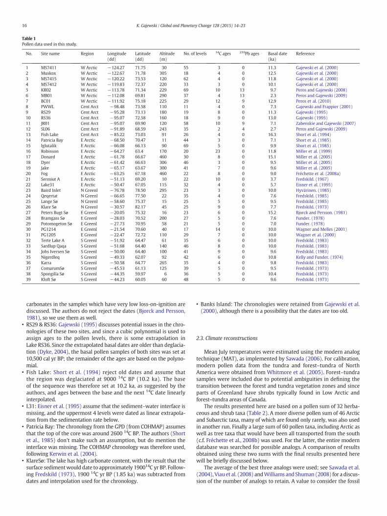
Table 1Pollen data used in this study.

No. Site name Region Longitude(dd)

Latitude(dd)

Altitude(m)

No. of levels 14C ages 210Pb ages Basal date(ka)

Reference

1 MS7411 W Arctic −124.27 71.75 30 55 3 0 11.3 Gajewski et al. (2000)2 Muskox W Arctic −122.67 71.78 305 18 4 0 12.5 Gajewski et al. (2000)3 MS7415 W Arctic −120.22 73.53 120 62 4 0 11.8 Gajewski et al. (2000)4 MS7412 W Arctic −119.83 72.37 220 33 3 0 10.1 Gajewski et al. (2000)5 KR02 W Arctic −113.78 71.34 229 69 10 13 9.7 Peros and Gajewski (2008)6 MB01 W Arctic −112.08 69.81 290 37 4 13 2.3 Peros and Gajewski (2009)7 BC01 W Arctic −111.92 75.18 225 29 12 9 12.9 Peros et al. (2010)8 PWWL Cent Arct −98.48 73.58 110 11 4 0 7.3 Gajewski and Frappier (2001)9 RS29 Cent Arct −95.28 73.13 180 19 8 0 11.3 Gajewski (1995)10 RS36 Cent Arct −95.07 72.58 160 18 9 0 13.0 Gajewski (1995)11 JR01 Cent Arct −95.07 69.90 120 58 10 9 7.1 Zabenskie and Gajewski (2007)12 SL06 Cent Arct −91.89 68.59 243 35 2 4 2.7 Peros and Gajewski (2009)13 Fish Lake Cent Arct −85.22 73.03 91 26 4 0 16.3 Short et al. (1994)14 Patricia Bay E Arctic −68.50 70.47 11 44 3 0 7.1 Short et al. (1985)15 Iglutalik E Arctic −66.08 66.13 90 69 5 0 9.9 Short et al. (1985)16 Robinson E Arctic −64.27 63.4 170 20 23 0 11.8 Miller et al. (1999)17 Donard E Arctic −61.78 66.67 460 30 8 0 15.1 Miller et al. (2005)18 Dyer E Arctic −61.42 66.63 306 46 3 0 9.5 Miller et al. (2005)19 Jake E Arctic −65.17 63.67 300 41 7 0 9.6 Miller et al. (2005)20 Fog E Arctic −63.25 67.18 460 22 8 0 9.0 Fréchette et al. (2008a)21 Sermiut A E Arctic −51.13 69.20 10 22 10 0 3.7 Fredskild. (1967)22 Lake31 E Arctic −50.47 67.05 115 32 4 0 5.7 Eisner et al. (1995)23 Baird Inlet N Greenl −76.78 78.50 295 23 3 0 10.0 Hyvärinen. (1985)24 Qeqertat N Greenl −66.65 77.50 22 35 4 0 7.6 Fredskild. (1985)25 Lange Sø N Greenl −58.60 75.37 15 25 5 0 9.5 Fredskild. (1985)26 Klare Sø N Greenl −30.57 82.17 45 25 9 0 7.7 Fredskild. (1973)27 Peters Bugt Sø E Greenl −20.05 75.32 16 23 6 0 15.2 Bjorck and Persson. (1981)28 Bramgass Sø E Greenl −28.03 70.52 200 27 5 0 7.6 Funder. (1978)29 Potomogeton Sø E Greenl −27.73 70.95 58 21 5 0 7.0 Funder. (1978)30 PG1214 E Greenl −21.54 70.60 40 17 14 0 10.0 Wagner and Melles (2001)31 PG1205 E Greenl −22.47 72.72 110 29 7 0 10.0 Wagner et al. (2000)32 Terte Lake A S Greenl −51.92 64.47 61 35 6 0 10.0 Fredskild. (1983)33 Sardlup Qaqa S Greenl −51.68 64.40 140 46 8 0 10.0 Fredskild. (1983)34 Johs Iversen Sø S Greenl −50.00 64.40 100 41 9 0 9.6 Fredskild. (1983)35 Nigerdleq S Greenl −49.33 62.07 92 42 6 0 10.8 Kelly and Funder. (1974)36 Karra S Greenl −50.58 64.77 265 35 4 0 9.8 Fredskild. (1983)37 ComarumSø S Greenl −45.53 61.13 125 39 5 0 9.5 Fredskild. (1973)38 Spongilla Sø S Greenl −44.35 59.97 6 36 5 0 10.4 Fredskild. (1973)39 Kloft Sø S Greenl −44.23 60.05 60 48 5 0 9.6 Fredskild. (1973)

16 K. Gajewski / Global and Planetary Change 128 (2015) 14–23

carbonates in the samples which have very low loss-on-ignition arediscussed. The authors do not reject the dates (Bjorck and Persson,1981), so we use them as well.

• RS29 & RS36: Gajewski (1995) discusses potential issues in the chro-nologies of these two sites, and since a cubic polynomial is used toassign ages to the pollen levels, there is some extrapolation inLake RS36. Since the extrapolated basal dates are older than deglacia-tion (Dyke, 2004), the basal pollen samples of both sites was set at10,500 cal yr BP; the remainder of the ages are based on the polyno-mial.

• Fish Lake: Short et al. (1994) reject old dates and assume thatthe region was deglaciated at 9000 14C BP (10.2 ka). The baseof the sequence was therefore set at 10.2 ka, as suggested by theauthors, and ages between the base and the next 14C date linearlyinterpolated.

• L31: Eisner et al. (1995) assume that the sediment–water interface ismissing, and the uppermost 4 levels were dated as linear extrapola-tion from the sedimentation rate below.

• Patricia Bay: The chronology from the GPD (from COHMAP) assumesthat the top of the core was around 2600 14C BP. The authors (Shortet al., 1985) don't make such an assumption, but do mention theinterface was missing. The COHMAP chronology was therefore used,following Kerwin et al. (2004).

• KlareSø: The lake has high carbonate content, with the result that thesurface sedimentwould date to approximately 190014C yr BP. Follow-ing Fredskild (1973), 1900 14C yr BP (1.85 ka) was subtracted fromdates and interpolation used for the chronology.

• Banks Island: The chronologies were retained from Gajewski et al.(2000), although there is a possibility that the dates are too old.

2.3. Climate reconstructions

Mean July temperatures were estimated using the modern analogtechnique (MAT), as implemented by Sawada (2006). For calibration,modern pollen data from the tundra and forest–tundra of NorthAmerica were obtained from Whitmore et al. (2005). Forest–tundrasamples were included due to potential ambiguities in defining thetransition between the forest and tundra vegetation zones and sinceparts of Greenland have shrubs typically found in Low Arctic andforest–tundra areas of Canada.

The results presented here are based on a pollen sum of 32 herba-ceous and shrub taxa (Table 2). A more diverse pollen sum of 46 Arcticand Subarctic taxa, many of which are found only rarely, was also usedin another run. Finally a large sum of 60 pollen taxa, including Arctic aswell as tree taxa that would have been all transported from the south(c.f. Fréchette et al., 2008b) was used. For the latter, the entire moderndatabase was searched for possible analogs. A comparison of resultsobtained using these two sums with the final results presented herewill be briefly discussed below.

The average of the best three analogs were used; see Sawada et al.(2004), Viau et al. (2008) andWilliams and Shuman (2008) for a discus-sion of the number of analogs to retain. A value to consider the fossil

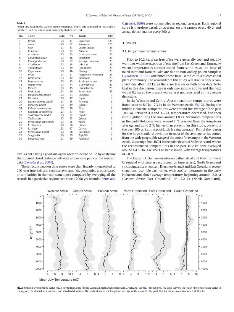
Table 2Pollen taxa used in the various reconstruction attempts. The sum used in this study isnumber 1, and the others were sensitivity studies; see text.

No. Taxon Sum No. Taxon Sum

1 Betula 123 31 Equisetum 1232 Alnus 123 32 Sphagnum 1233 Salix 123 33 Cupressaceae 234 Ericaceae 123 34 Armeria 235 Artemisia 123 35 Campanulaceae 236 Caryophyllaceae 123 36 Epilobium 237 Chenopodiaceae 123 37 Koenigia islandica 238 Cruciferae 123 38 Labiatae 239 Tubuliflorae 123 39 Liguliflorae 2310 Cyperaceae 123 40 Plantago 2311 Dryas 123 41 Polygonum viviparum 2312 Gramineae 123 42 Rubiaceae 2313 Leguminosae 123 43 Saxifraga cernua 2314 Oxyria-type 123 44 S. hieracifolia 2315 Papaver 123 45 Umbelliferae 2316 Pedicularis 123 46 Botrychium 2319 Polygonaceae undiff 123 54 Castanea 323 Potentilla 123 47 Fagus 320 Ranunculaceae undiff 123 48 Fraxinus 322 Rosaceae undiff 123 49 Juglans 324 Rubus chamaemorus 123 50 Picea 317 Saxifraga oppositifolia 123 51 Pinus 318 Saxifragaceae undiff 123 52 Populus 321 Thalictrum 123 53 Quercus 325 Lycopodium annotinum 123 55 Tsuga 326 L. clavatum 123 56 Ulmus 327 L. selago 123 57 Corylus 328 Lycopodium undiff 123 58 Juncaceae 329 Selaginella 123 59 Tofieldia 330 Polypodiaceae 123 60 Pteridium 3

17K. Gajewski / Global and Planetary Change 128 (2015) 14–23

level as not having a good analogwasdetermined to be 0.2, by analyzingthe squared chord distance between all possible pairs of the moderndata (Sawada et al., 2004).

These reconstruction time series were then linearly interpolated to200-year intervals and regional averages (six geographic groups basedon similarities in the reconstructions) computed by averaging all therecords in a particular region; two short (2000 yr) records (Peros and

0

1000

2000

3000

4000

5000

6000

7000

8000

9000

10000

caly

rBP

Mean July Temperature (oC)

4 6 8 10 2 4 6 8 4 6 8 10

Western Arctic Central Arctic Eastern Arctic

Fig. 2. Regional average time seriesmean July temperature for the Canadian Arctic Archipelagothe region; the shaded area encloses one standard deviation. The vertical line is the long-term

Gajewski, 2009) were not included in regional averages. Each regionalcurve is therefore based, on average, on one sample every 40 yr andan age determination every 200 yr.

3. Results

3.1. Temperature reconstructions

Prior to 10.2 ka, areas free of ice were generally cool and steadilywarming, with the exception of one site from East Greenland. Unusuallywarm temperatures reconstructed from samples at the base ofBaird Inlet and Donard Lake are due to non-analog pollen samples;Hyvärinen (1985) attributes these basal samples to a successionalplant community. The remainder of this study will discuss only recon-structions after 10.2 ka, as there are few series with older data. Notethat in this discussion, there is only one sample at 0 ka and the nextwas at 0.2 ka, so the present warming is not registered in the averagedepictions.

In the Western and Central Arctic, maximum temperatures werefound prior to 8.0 ka (7.3 ka in the Western Arctic; Fig. 2). During themiddle Holocene, temperatures were around the average of the past10.2 ka. Between 4.0 and 3.6 ka, temperatures decreased, and thenrose slightly during the time around 1.0 ka. Maximum temperaturesin the early Holocene were around 1 °C warmer than the long-termaverage and up to 2 °C higher than present (in this study, present isthe past 100 yr, i.e., the post-Little Ice Age average). Part of the reasonfor the large standard deviation in most of the average series comesfrom thewide geographic range of the cores; for example in theWesternArctic, sites range fromBC01 in the polar desert ofMelville Island,wherethe reconstructed temperatures in the past 10.2 ka have averagedaround 4.4 °C, to LakeMS11 on Banks Island, with average temperaturesof 7.8 °C.

The Eastern Arctic (seven sites on Baffin Island and two from westGreenland with similar reconstruction time series), North Greenland(including a site on eastern Ellesmere Island) and East Greenland recon-structions resemble each other, with cool temperatures in the earlyHolocene and above average temperatures beginning around ~8.0 ka(Eastern Arctic, East Greenland) or ~7.2 ka (North Greenland).

2 4 6 8 2 4 6 8 4 6 8 10

0

1000

2000

3000

4000

5000

6000

7000

8000

9000

10000

North Greenland East Greenland South Greenland

andGreenland; see Fig. 1 for regions. The solid curve is themean July temperature series inaverage of the curve for the past 10.2 ka. Curves were truncated at 10.2 ka.

18 K. Gajewski / Global and Planetary Change 128 (2015) 14–23

Temperatures return to average ~5.2 ka, and decrease slightly in thepast 1.8 ka. In the Central Arctic, Eastern Arctic and North Greenland,present conditions are near the mean temperature of the past 10.2 ka,whereas in the Western Arctic and East Greenland, the past 200 yr arethe coldest of the past 8000 yr.

In South Greenland, the average temperature curve shows a long-term warming trend between 10.2 ka to 3.2 ka, a slight cooling until2.8 ka and stable temperatures subsequently. Lowest temperatures ofthe Holocene in this region were over 2 °C cooler than present. Thisrelatively small area is served by eight pollen diagrams, and all havesimilar reconstructions, leading to an average reconstruction with asmall standard deviation (Fig. 2).

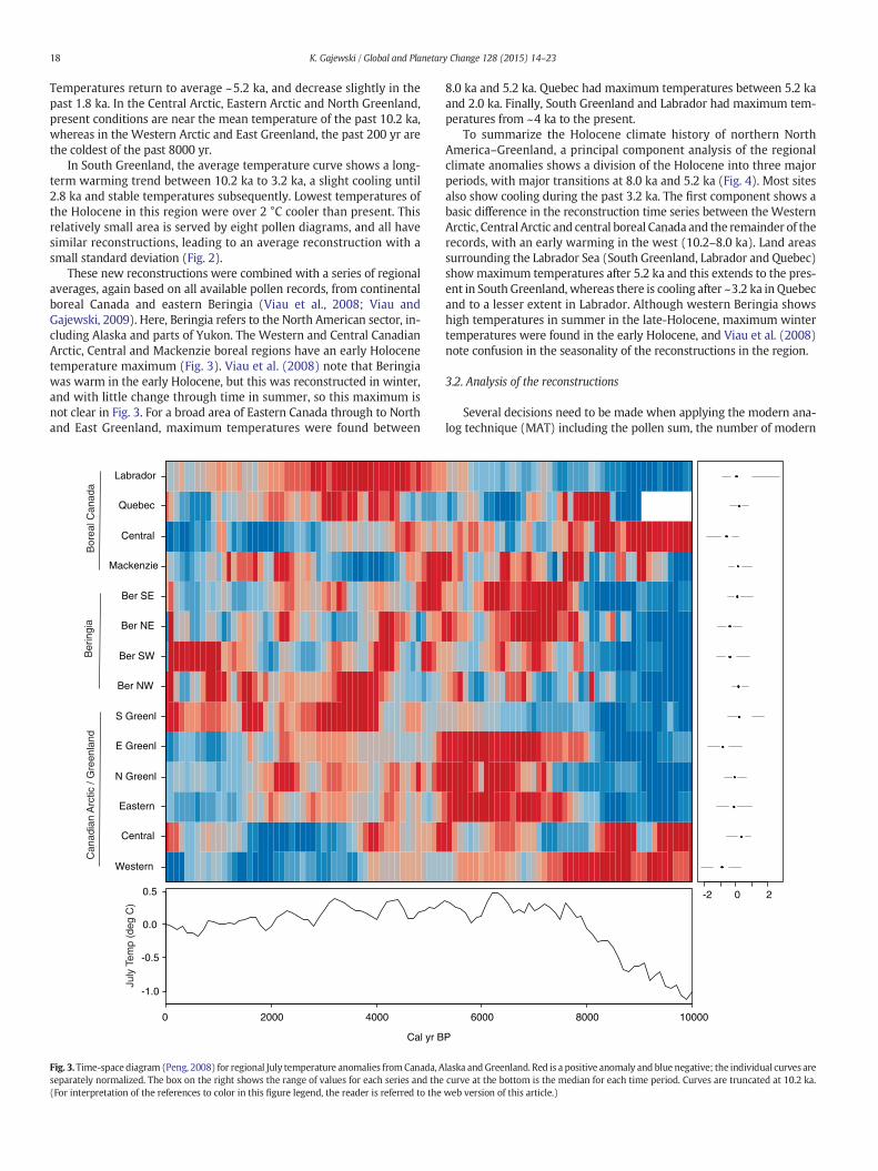
These new reconstructions were combined with a series of regionalaverages, again based on all available pollen records, from continentalboreal Canada and eastern Beringia (Viau et al., 2008; Viau andGajewski, 2009). Here, Beringia refers to the North American sector, in-cluding Alaska and parts of Yukon. The Western and Central CanadianArctic, Central and Mackenzie boreal regions have an early Holocenetemperature maximum (Fig. 3). Viau et al. (2008) note that Beringiawas warm in the early Holocene, but this was reconstructed in winter,and with little change through time in summer, so this maximum isnot clear in Fig. 3. For a broad area of Eastern Canada through to Northand East Greenland, maximum temperatures were found between

Western

Central

Eastern

N Greenl

E Greenl

S Greenl

Ber NW

Ber SW

Ber NE

Ber SE

Mackenzie

Central

Quebec

Labrador

-1.0

-0.5

0.0

0.5

0 2000 4000

adanaClaero

Baignire

Bnaidana

Cdnalneer

G/citcr

A

)C

ged(p

meTyluJ

Cal yr B

Fig. 3.Time-space diagram (Peng, 2008) for regional July temperature anomalies fromCanada, Aseparately normalized. The box on the right shows the range of values for each series and the(For interpretation of the references to color in this figure legend, the reader is referred to the

8.0 ka and 5.2 ka. Quebec had maximum temperatures between 5.2 kaand 2.0 ka. Finally, South Greenland and Labrador had maximum tem-peratures from ~4 ka to the present.

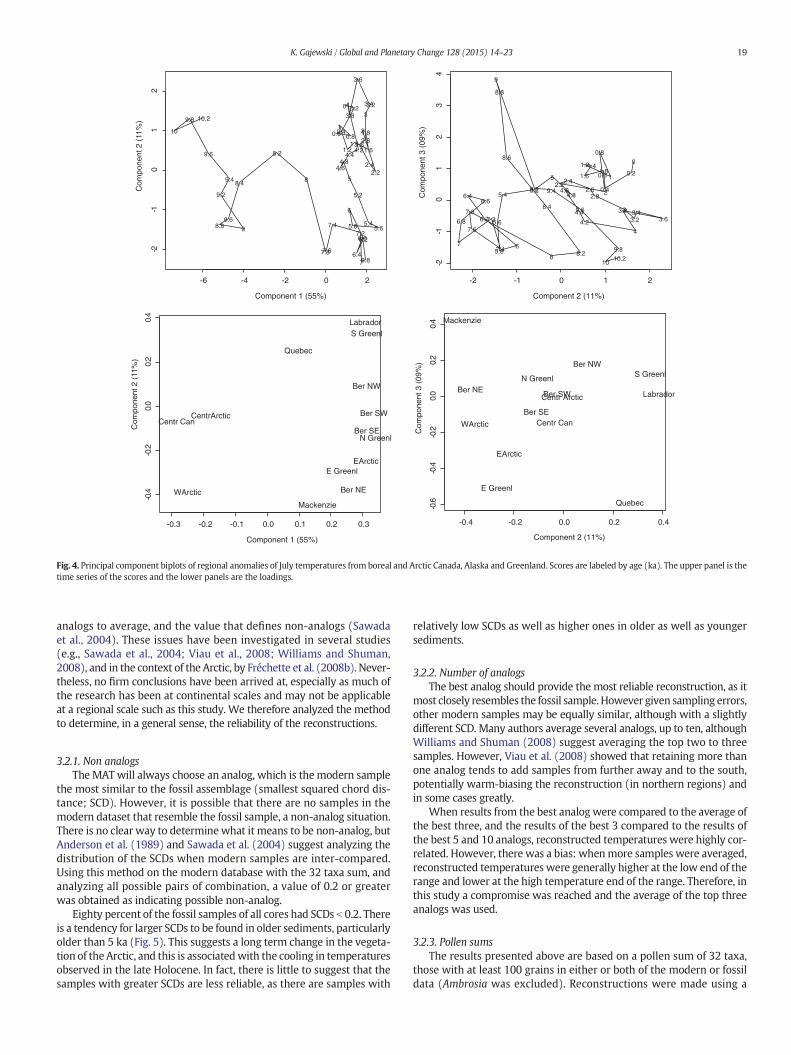
To summarize the Holocene climate history of northern NorthAmerica–Greenland, a principal component analysis of the regionalclimate anomalies shows a division of the Holocene into three majorperiods, with major transitions at 8.0 ka and 5.2 ka (Fig. 4). Most sitesalso show cooling during the past 3.2 ka. The first component shows abasic difference in the reconstruction time series between theWesternArctic, Central Arctic and central boreal Canada and the remainder of therecords, with an early warming in the west (10.2–8.0 ka). Land areassurrounding the Labrador Sea (South Greenland, Labrador and Quebec)showmaximum temperatures after 5.2 ka and this extends to the pres-ent in South Greenland, whereas there is cooling after ~3.2 ka in Quebecand to a lesser extent in Labrador. Although western Beringia showshigh temperatures in summer in the late-Holocene, maximum wintertemperatures were found in the early Holocene, and Viau et al. (2008)note confusion in the seasonality of the reconstructions in the region.

3.2. Analysis of the reconstructions

Several decisions need to be made when applying the modern ana-log technique (MAT) including the pollen sum, the number of modern

-2 0 2

6000 8000 10000

P

laska andGreenland. Red is a positive anomaly and blue negative; the individual curves arecurve at the bottom is the median for each time period. Curves are truncated at 10.2 ka.web version of this article.)

-2-1

01

2

Component 1 (55%)

0 0.2

0.40.6 0.8

1

1.21.4

1.6

1.82

2.22.4

2.62.8

3

3.23.4

3.6

3.8

4

4.24.4

4.64.8

5

5.2

5.45.65.8

6

6.2

6.4

6.6

6.87

7.27.4

7.67.8

8

8.2

8.4

8.68.8 9

9.2

9.4

9.6

9.8

10

10.2

1(2tnenop

moC

)%1

Component 1 (55%)

WArctic

CentrArctic

EArctic

N Greenl

E Greenl

S Greenl

Ber NW

Ber SW

Ber NE

Ber SE

Mackenzie

Centr Can

Quebec

Labrador

1(2tnenop

moC

)%1

-2-1

01

23

4

Component 2 (11%)

0

0.2

0.4

0.6

0.8

1

1.21.4

1.61.8

22.22.4

2.62.8

3

3.23.4

3.63.8

44.2

4.4

4.64.8

5

5.25.4

5.6

5.86

6.2

6.46.6

6.8

7

7.2

7.4

7.6

7.8

8 8.2

8.4

8.6

8.8

9

9.2 9.4

9.6

9.8

1010.2

)%90(

3tnenopmo

C

-6 -4 -2 0 2

-0.3 -0.2 -0.1 0.0 0.1 0.2 0.3

-2 -1 0 1 2

-0.4 -0.2 0.0 0.2 0.4

-0.4

-0.2

0.0

0.2

0.4

-0.6

-0.4

-0.2

0.0

0.2

0.4

Component 2 (11%)

WArctic

Centr Arctic

EArctic

N Greenl

E Greenl

S GreenlBer NW

Ber SWBer NE

Ber SE

Mackenzie

Centr Can

Quebec

Labrador

)%90(

3tnenopmo

C

Fig. 4. Principal component biplots of regional anomalies of July temperatures from boreal and Arctic Canada, Alaska and Greenland. Scores are labeled by age (ka). The upper panel is thetime series of the scores and the lower panels are the loadings.

19K. Gajewski / Global and Planetary Change 128 (2015) 14–23

analogs to average, and the value that defines non-analogs (Sawadaet al., 2004). These issues have been investigated in several studies(e.g., Sawada et al., 2004; Viau et al., 2008; Williams and Shuman,2008), and in the context of the Arctic, by Fréchette et al. (2008b). Never-theless, no firm conclusions have been arrived at, especially as much ofthe research has been at continental scales and may not be applicableat a regional scale such as this study. We therefore analyzed the methodto determine, in a general sense, the reliability of the reconstructions.

3.2.1. Non analogsThe MAT will always choose an analog, which is themodern sample

the most similar to the fossil assemblage (smallest squared chord dis-tance; SCD). However, it is possible that there are no samples in themodern dataset that resemble the fossil sample, a non-analog situation.There is no clear way to determinewhat it means to be non-analog, butAnderson et al. (1989) and Sawada et al. (2004) suggest analyzing thedistribution of the SCDs when modern samples are inter-compared.Using this method on the modern database with the 32 taxa sum, andanalyzing all possible pairs of combination, a value of 0.2 or greaterwas obtained as indicating possible non-analog.

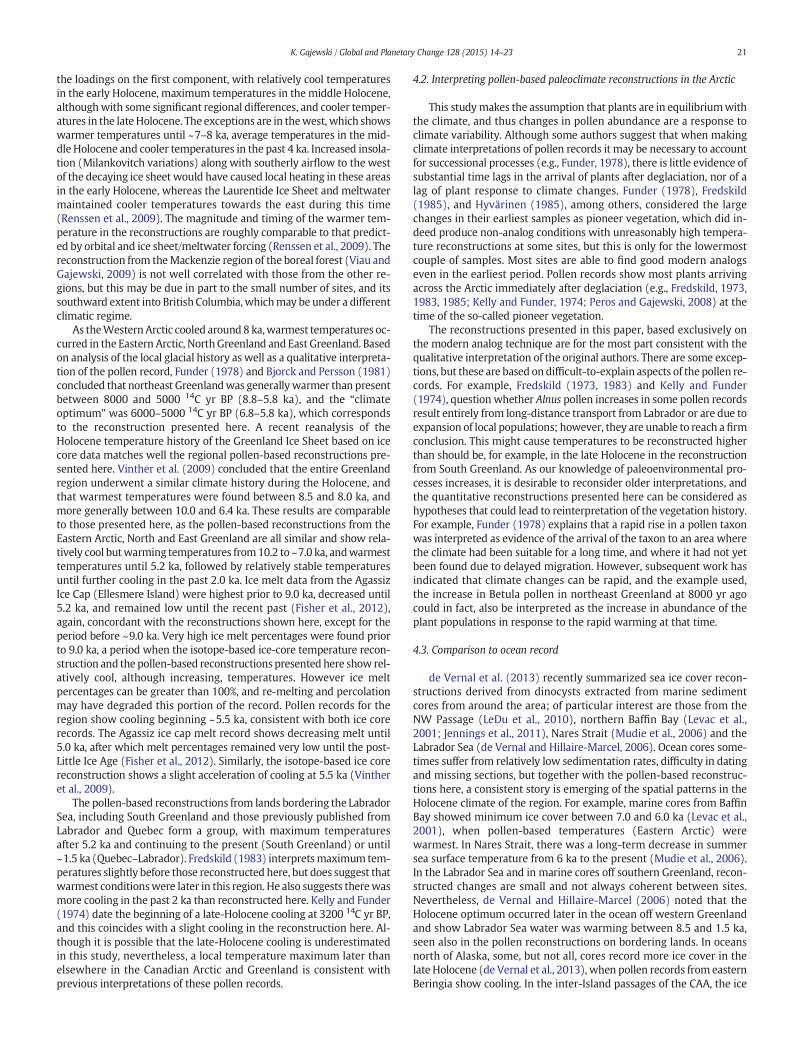
Eighty percent of the fossil samples of all cores had SCDs b 0.2. Thereis a tendency for larger SCDs to be found in older sediments, particularlyolder than 5 ka (Fig. 5). This suggests a long term change in the vegeta-tion of the Arctic, and this is associatedwith the cooling in temperaturesobserved in the late Holocene. In fact, there is little to suggest that thesamples with greater SCDs are less reliable, as there are samples with

relatively low SCDs as well as higher ones in older as well as youngersediments.

3.2.2. Number of analogsThe best analog should provide the most reliable reconstruction, as it

most closely resembles the fossil sample. However given sampling errors,other modern samples may be equally similar, although with a slightlydifferent SCD. Many authors average several analogs, up to ten, althoughWilliams and Shuman (2008) suggest averaging the top two to threesamples. However, Viau et al. (2008) showed that retaining more thanone analog tends to add samples from further away and to the south,potentially warm-biasing the reconstruction (in northern regions) andin some cases greatly.

When results from the best analog were compared to the average ofthe best three, and the results of the best 3 compared to the results ofthe best 5 and 10 analogs, reconstructed temperatures were highly cor-related. However, there was a bias: whenmore samples were averaged,reconstructed temperatures were generally higher at the low end of therange and lower at the high temperature end of the range. Therefore, inthis study a compromise was reached and the average of the top threeanalogs was used.

3.2.3. Pollen sumsThe results presented above are based on a pollen sum of 32 taxa,

those with at least 100 grains in either or both of the modern or fossildata (Ambrosia was excluded). Reconstructions were made using a

0

1000

2000

3000

4000

5000

6000

7000

8000

9000

10000

PB

rylac

40 80

DC

S

5

setiS

#

40 80

DC

S

5

setiS

#

40 80

DC

S

5seti

S#

40 80

DC

S

5

setiS

#

40 80

DC

S

5

setiS

#

40 80

DC

S

5

setiS

#

WesternArctic

CentralArctic

EasternArctic

NorthGreenland

EastGreenland

SouthGreenland

Fig. 5. Values of squared chord distance (SCD; multiplied by 100) for all pollen spectra and number of sites used to compute the regional curves shown in Fig. 2.

20 K. Gajewski / Global and Planetary Change 128 (2015) 14–23

second pollen sum, containing 46 taxa, including shrubs, non-arborealpollen (NAP — herbaceous plants) and spores of plants that would beexpected to grow in the Arctic. Some of these taxa were very rare, how-ever, in either the fossil or the modern datasets. Again modern calibra-tion samples included only data from the “Arctic” and “forest–tundra”vegetation zones. This attempt was used to see if rare taxa could refinethe reconstructions in spite of the greater error in estimating the abun-dance and spatial distribution of the pollen taxa.

The reconstructed July temperatures, when using the 32 and 46taxon sums, were highly correlated; 87% chose the same sample asthe best analog (or a sample that gave an identical temperature), and97% chose analogs that gave reconstructed temperatures within 1 °Cof each other. There was no tendency for relatively large reconstructedtemperature differences to be concentrated at any one time period.SCDs were also similar: 78% (46 taxon sum) and 79% (32 taxon sum)gave SCDs less than 0.2. The difference in the SCDs between the 46taxon and 32 taxon sums was also small: 30% was zero and 67% wasless than 0.05. Most of the larger SCD differences were found in threelakes: Johannes Iverson Sø, Comarum Sø and Karra, and tended to befound between 4 and 7 ka and around 10 ka. Increasing the sum of Arc-tic pollen taxa therefore made little improvement or difference in thereconstructions or in finding analogs, although it maymake a differencein some individual sites.

Finally, a large sumof 60 tree (arboreal pollen;AP), shrub andherba-ceous pollen taxa (NAP), Pteridophyte and Sphagnum spores was used;this was attempted for comparisonwith previous studies (Sawada et al.,2004; Fréchette et al., 2008b). Taxa with fewer than 10 pollen grains inthe fossil dataset were excluded. The calibration area included all ofNorth America, that is, the database of Whitmore et al. (2005).

When the reconstructions using this pollen sum were compared tothose of the 32 taxa, the results were again broadly correlated, however,therewere a number of relatively high July temperatures. This time, 55%of the samples found the same analog, and 80% reconstructed tempera-tures within 1 °C of that reconstructed using the 32 taxa sum.More fos-sil samples were reconstructed warmer (34%) than colder (11%) usingtheAP+NAP sum. Thus, therewas a distinct bias towardswarmer tem-peratures; the warmer temperatures using the AP + NAP sum were

found evenly throughout the entire time period. The difference betweenthe two reconstructions could be up to 18 °C; however, large differenceswere concentrated in several sites. For example, although most of thereconstructions were identical or similar, Fish Lake and Sardlup hadsections that were distinctly warmer using the AP + NAP sum andSermiut, JR01, MB01 and PG14 were almost entirely reconstructedwarmer. In KR02, the period of time older than 8 ka was, however,reconstructed colder using the AP + NAP sum.

Using such a large sum has the potential to better distinguish be-tween samples from different regions, but in Arctic lake sediments,windblown pollen from forested areas to the south can comprise alarge proportion of the pollen rain (Fredskild, 1973; Nichols et al.,1978; Ritchie et al., 1987; Gajewski, 1995, 2002; Fréchette et al.,2008b). Fréchette et al. (2008b) retained them in their reconstructions.However, since these pollen come fromplants that never grew in the re-gion surrounding the sites, it is not clear how these are to be interpreted.Given these results, the use of AP + NAP sums for reconstructingclimate from Arctic samples is not encouraged.

4. Discussion

4.1. Summary of Holocene climate changes

These results permit, for the first time, an analysis of the Holoceneclimates across the entire North American Arctic and Subarctic, includ-ing coastal Greenland. These reconstructions are based on one proxy,pollen data, which has the advantage of providing comparable recon-structions along a large area, although with the potential biases andissues of any one proxy. The ecology of Arctic plants is relatively well-known, and plant distribution and production are clearly affected bytemperatures during the short, snow-free summer season. Gajewski(2002) and Kerwin et al. (2004) have shown that the modern pollenassemblages from the Canadian Arctic correspond well with the localvegetation and that differences in pollen percentages can be used to dis-tinguish the major regions and vegetation zones.

Most of the series of the Holocene temperatures from the CanadianArctic and Greenland show a broad-scale similarity, as expressed in

21K. Gajewski / Global and Planetary Change 128 (2015) 14–23

the loadings on the first component, with relatively cool temperaturesin the early Holocene, maximum temperatures in the middle Holocene,althoughwith some significant regional differences, and cooler temper-atures in the late Holocene. The exceptions are in thewest, which showswarmer temperatures until ~7–8 ka, average temperatures in the mid-dle Holocene and cooler temperatures in the past 4 ka. Increased insola-tion (Milankovitch variations) along with southerly airflow to the westof the decaying ice sheet would have caused local heating in these areasin the early Holocene, whereas the Laurentide Ice Sheet and meltwatermaintained cooler temperatures towards the east during this time(Renssen et al., 2009). The magnitude and timing of the warmer tem-perature in the reconstructions are roughly comparable to that predict-ed by orbital and ice sheet/meltwater forcing (Renssen et al., 2009). Thereconstruction from theMackenzie region of the boreal forest (Viau andGajewski, 2009) is not well correlated with those from the other re-gions, but this may be due in part to the small number of sites, and itssouthward extent into British Columbia,whichmay be under a differentclimatic regime.

As theWestern Arctic cooled around 8 ka,warmest temperatures oc-curred in the Eastern Arctic, NorthGreenland and East Greenland. Basedon analysis of the local glacial history as well as a qualitative interpreta-tion of the pollen record, Funder (1978) and Bjorck and Persson (1981)concluded that northeast Greenlandwas generallywarmer than presentbetween 8000 and 5000 14C yr BP (8.8–5.8 ka), and the “climateoptimum” was 6000–5000 14C yr BP (6.8–5.8 ka), which correspondsto the reconstruction presented here. A recent reanalysis of theHolocene temperature history of the Greenland Ice Sheet based on icecore data matches well the regional pollen-based reconstructions pre-sented here. Vinther et al. (2009) concluded that the entire Greenlandregion underwent a similar climate history during the Holocene, andthat warmest temperatures were found between 8.5 and 8.0 ka, andmore generally between 10.0 and 6.4 ka. These results are comparableto those presented here, as the pollen-based reconstructions from theEastern Arctic, North and East Greenland are all similar and show rela-tively cool butwarming temperatures from10.2 to ~7.0 ka, andwarmesttemperatures until 5.2 ka, followed by relatively stable temperaturesuntil further cooling in the past 2.0 ka. Ice melt data from the AgassizIce Cap (Ellesmere Island) were highest prior to 9.0 ka, decreased until5.2 ka, and remained low until the recent past (Fisher et al., 2012),again, concordant with the reconstructions shown here, except for theperiod before ~9.0 ka. Very high ice melt percentages were found priorto 9.0 ka, a period when the isotope-based ice-core temperature recon-struction and the pollen-based reconstructionspresented here show rel-atively cool, although increasing, temperatures. However ice meltpercentages can be greater than 100%, and re-melting and percolationmay have degraded this portion of the record. Pollen records for theregion show cooling beginning ~5.5 ka, consistent with both ice corerecords. The Agassiz ice cap melt record shows decreasing melt until5.0 ka, after which melt percentages remained very low until the post-Little Ice Age (Fisher et al., 2012). Similarly, the isotope-based ice corereconstruction shows a slight acceleration of cooling at 5.5 ka (Vintheret al., 2009).

The pollen-based reconstructions from lands bordering the LabradorSea, including South Greenland and those previously published fromLabrador and Quebec form a group, with maximum temperaturesafter 5.2 ka and continuing to the present (South Greenland) or until~1.5 ka (Quebec–Labrador). Fredskild (1983) interpretsmaximum tem-peratures slightly before those reconstructed here, but does suggest thatwarmest conditionswere later in this region. He also suggests therewasmore cooling in the past 2 ka than reconstructed here. Kelly and Funder(1974) date the beginning of a late-Holocene cooling at 3200 14C yr BP,and this coincides with a slight cooling in the reconstruction here. Al-though it is possible that the late-Holocene cooling is underestimatedin this study, nevertheless, a local temperature maximum later thanelsewhere in the Canadian Arctic and Greenland is consistent withprevious interpretations of these pollen records.

4.2. Interpreting pollen-based paleoclimate reconstructions in the Arctic

This studymakes the assumption that plants are in equilibriumwiththe climate, and thus changes in pollen abundance are a response toclimate variability. Although some authors suggest that when makingclimate interpretations of pollen records it may be necessary to accountfor successional processes (e.g., Funder, 1978), there is little evidence ofsubstantial time lags in the arrival of plants after deglaciation, nor of alag of plant response to climate changes. Funder (1978), Fredskild(1985), and Hyvärinen (1985), among others, considered the largechanges in their earliest samples as pioneer vegetation, which did in-deed produce non-analog conditions with unreasonably high tempera-ture reconstructions at some sites, but this is only for the lowermostcouple of samples. Most sites are able to find good modern analogseven in the earliest period. Pollen records show most plants arrivingacross the Arctic immediately after deglaciation (e.g., Fredskild, 1973,1983, 1985; Kelly and Funder, 1974; Peros and Gajewski, 2008) at thetime of the so-called pioneer vegetation.

The reconstructions presented in this paper, based exclusively onthe modern analog technique are for the most part consistent with thequalitative interpretation of the original authors. There are some excep-tions, but these are based on difficult-to-explain aspects of the pollen re-cords. For example, Fredskild (1973, 1983) and Kelly and Funder(1974), question whether Alnus pollen increases in some pollen recordsresult entirely from long-distance transport from Labrador or are due toexpansion of local populations; however, they are unable to reach a firmconclusion. This might cause temperatures to be reconstructed higherthan should be, for example, in the late Holocene in the reconstructionfrom South Greenland. As our knowledge of paleoenvironmental pro-cesses increases, it is desirable to reconsider older interpretations, andthe quantitative reconstructions presented here can be considered ashypotheses that could lead to reinterpretation of the vegetation history.For example, Funder (1978) explains that a rapid rise in a pollen taxonwas interpreted as evidence of the arrival of the taxon to an area wherethe climate had been suitable for a long time, and where it had not yetbeen found due to delayed migration. However, subsequent work hasindicated that climate changes can be rapid, and the example used,the increase in Betula pollen in northeast Greenland at 8000 yr agocould in fact, also be interpreted as the increase in abundance of theplant populations in response to the rapid warming at that time.

4.3. Comparison to ocean record

de Vernal et al. (2013) recently summarized sea ice cover recon-structions derived from dinocysts extracted from marine sedimentcores from around the area; of particular interest are those from theNW Passage (LeDu et al., 2010), northern Baffin Bay (Levac et al.,2001; Jennings et al., 2011), Nares Strait (Mudie et al., 2006) and theLabrador Sea (de Vernal and Hillaire-Marcel, 2006). Ocean cores some-times suffer from relatively low sedimentation rates, difficulty in datingand missing sections, but together with the pollen-based reconstruc-tions here, a consistent story is emerging of the spatial patterns in theHolocene climate of the region. For example, marine cores from BaffinBay showed minimum ice cover between 7.0 and 6.0 ka (Levac et al.,2001), when pollen-based temperatures (Eastern Arctic) werewarmest. In Nares Strait, there was a long-term decrease in summersea surface temperature from 6 ka to the present (Mudie et al., 2006).In the Labrador Sea and in marine cores off southern Greenland, recon-structed changes are small and not always coherent between sites.Nevertheless, de Vernal and Hillaire-Marcel (2006) noted that theHolocene optimum occurred later in the ocean off western Greenlandand show Labrador Sea water was warming between 8.5 and 1.5 ka,seen also in the pollen reconstructions on bordering lands. In oceansnorth of Alaska, some, but not all, cores record more ice cover in thelate Holocene (de Vernal et al., 2013), when pollen records from easternBeringia show cooling. In the inter-Island passages of the CAA, the ice

22 K. Gajewski / Global and Planetary Change 128 (2015) 14–23

cover record is not as clear, as there are probably large regional differ-ences; in addition ice cover depends partly on currents and, in theearly Holocene, from ice supply by the melting ice sheets (Dyke et al.,1996a,b, 1997; LeDu et al., 2010). Using ocean sediment cores fromseveral areas, Cronin et al. (2010) note that the Arctic Ocean was sea-sonally ice-free during the late-Glacial through to 5.0–6.0 ka. Theseare not clearly dated, and suffer from very low sedimentation rates;and they note there may be regional differences. This generally con-cords with the reconstructions presented here, which show warmesttemperatures prior to ~5 ka, although not in all regions simultaneously,nor necessarily throughout the time period.

These results show the postglacial temperature history of the areathat had been covered by the Laurentide, Innuitian, Greenland andCordilleran Ice Sheets during the full glacial. The principal componentsanalysis shows a division of the Holocene into three major periods,with major transitions at 8.0 ka and 5.2 ka;most sites also show coolingduring the past 3.2 ka. The results of this study are concordant withthose from ice cores, and generally in agreement with sea ice cover re-constructions from ocean cores, although the latter are also affectedby ocean currents and ice export or import into the region. Most ofthe Arctic had maximum temperatures shortly after the collapse of theLaurentide Ice Sheet (8.2 ka), as insolation was higher and the IceSheet was no longer influencing the regional climate. In the westernand central Arctic, maximum temperatures were found earlier whereasthey were later in areas surrounding the Labrador Sea.

Acknowledgments

The data from this study are available at the NOAA PaleoclimatologyDatabase (www.ncdc.noaa.gov/paleo). This study was supported bythe Natural Sciences and Engineering Research Council of Canada. J.Whitmore, C. Rogers and M. Chaput helped in data entry, file organiza-tion and figure preparation. We acknowledge authors who providedpollen counts or other data, especially B. Fredskild, H. Hyvarinen, S.Funder, B. Fréchette, M. Kerwin, D. LeDu and A. de Vernal. Thanks totwo anonymous reviewers for comments.

References

Anderson, P., Bartlein, P., Brubaker, L., Gajewski, K., Ritchie, J., 1989. Modern analogues oflate-Quaternary pollen spectra from the western interior of North America.J. Biogeogr. 16, 573–596. http://dx.doi.org/10.2307/2845212.

Bjorck, S., Persson, T., 1981. LateWeichselian and Flandrian biostratigraphy and chronologyfrom Hochstetter Forland, Northeast Greenland. Medd. Gronl. Geosci. 5, 1–19.

Brandt, J.P., 2009. The extent of the North American boreal zone. Environ. Rev. 17,101–161. http://dx.doi.org/10.1139/A09-004.

CAPE Project Members, 2001. Holocene paleoclimate data from the Arctic: testing modelsof global climate change. Quat. Sci. Rev. 20, 1275–1287. http://dx.doi.org/10.1016/S0277-3791(01)00010-5.

CAVM Team. 2003. Circumpolar Arctic Vegetation Map. (1:7,500,000 scale), Conservationof Arctic Flora and Fauna (CAFF)Map No. 1. U.S. Fish andWildlife Service, Anchorage,Alaska. http://www.geobotany.uaf.edu/cavm/.

Cronin, L.M., Gemery, L., Briggs Jr., W., Jakobsson, M., Polyak, L., Brouwers, E., 2010. Qua-ternary sea-ice history in the Arctic Ocean based on a new Ostracode sea-ice proxy.Quat. Sci. Rev. 29, 3415–3429. http://dx.doi.org/10.1016/j.quascirev.2010.05.024.

deVernal, A., Hillaire-Marcel, C., 2006. Provincialism in trends and high frequency changesin eh northwest North Atlantic during the Holocene. Global Planet. Chang. 54,263–290. http://dx.doi.org/10.1016/j.gloplacha.2006.06.023.

de Vernal, A., Hillaire-Marcel, C., Rochon, A., Fréchette, B., Henry, M., Solignac, S., Bonnet,S., 2013. Dinocyst-based reconstructions of sea ice cover concentration during theHolocene in the Arctic Ocean, the northern North Atlantic Ocean and adjacent seas.Quat. Sci. Rev. 79, 111–121. http://dx.doi.org/10.1016/j.quascirev.2013.07.006.

Dyke, A.S., 2004. An outline of the deglaciation of North America with emphasis on centraland northern Canada. In: Ehlers, J., Gibbard, P.L. (Eds.), Quaternary Glaciations, Extentand Chronology. Part II. North America. Elsevier, Amsterdam, pp. 371–406.

Dyke, A.S., Dale, J., McNeely, R., 1996a. Marine molluscs as indicators of environmentalchange in glaciated North America and Greenland during the last 18,000 years.Géogr. Phys. Quat. 50, 125–184.

Dyke, A.S., Hooper, J., Savelle, J., 1996b. A history of sea ice in the Canadian Arctic Archi-pelago based on postglacial remains of bowhead whale (Balaena mysticetus). Arctic49, 235–255.

Dyke, A.S., England, J., Reimnitz, E., Jetté, H., 1997. Changes in driftwood delivery to theCanadianArcticArchipelago: thehypothesis of postglacial oscillationsof the transpolardrift. Arctic 50, 1–16.

Eisner,W.R., Tornqvist, T.E., Koster, E.A., Bennike, O., van Leeuwen, J.F., 1995. Paleoecologicalstudies of a Holocene lacustrine record from the Kangerlussuaq (Søndre Strømfjord)region of West Greenland. Quat. Res. 43 (1), 55–66. http://dx.doi.org/10.1006/qres.1995.1006.

Fisher, D., Zheng, J., Burgess, D., Zdanowicz, C., Kinnard, C., Sharp, M., Bourgeois, J., 2012.Recent melt rates of Canadian arctic ice caps are the highest in four millennia. GlobalPlanet. Chang. 84–85, 3–7. http://dx.doi.org/10.1016/j.gloplacha.2011.06.005.

Fréchette, B., de Vernal, A., 2009. Relationship between Holocene climate variations oversouthern Greenland and eastern Baffin Island and synoptic circulation pattern. Clim.Past 5, 347–359. http://dx.doi.org/10.5194/cp-5-347-2009.

Fréchette, B., Wolfe, A.P., Miller, G.H., Richard, P.J.H., de Vernal, A., 2006. Vegetation andclimate of the last interglacial on Baffin Island, Arctic Canada. Palaeogeogr.Palaeoclimatol. Palaeoecol. 236, 91–106. http://dx.doi.org/10.1016/j.palaeo.2005.11.034.

Fréchette, B., deVernal, A., Richard, P.J.H., 2008a. Holocene and last interglacial cloudinessin eastern Baffin Island, Arctic Canada. Can. J. Earth Sci. 45, 1221–1234. http://dx.doi.org/10.1139/E08-053.

Fréchette, B., de Vernal, A., Guiot, J., Wolfe, A., Miller, G., Fredskild, B., Kerwin, M., Richard,P., 2008b. Methodological basis for quantitative reconstruction of air temperatureand sunshine from pollen assemblages in Arctic Canada and Greenland. Quat. Sci.Rev. 27, 1197–1216. http://dx.doi.org/10.1016/j.quascirev.2008.02.016.

Fredskild, B., 1967. Palaeobotanical investigations at Sermermiutm Jakobshavn, westGreenland. Medd. Gronl. 178, 1–54.

Fredskild, B., 1973. Studies of the vegetational history of Greenland, palaeobotanicalinvestigation of some Holocene lake and bog deposits. Medd. Gronl. 198, 1–245.

Fredskild, B., 1983. The Holocene vegetational development of the Godthåbsfjord area,west Greenland. Medd. Gronl. Geosci. 10, 1–28.

Fredskild, B., 1985. The Holocene vegetational development of Tugtuligssuaq andQeqertat, northwest Greenland. Medd. Gronl. Geosci. 14, 1–20.

Funder, S., 1978. Holocene stratigraphy and vegetation history in the Scoresby Sund area,East Greenland. Grønl. Geol. Unders. 12, 1–66.

Gajewski, K., 1995. Modern and Holocene pollen assemblages from some small arcticlakes on Somerset Island, N.W.T., Canada. Quat. Res. 44, 228–236. http://dx.doi.org/10.1006/qres.1995.1067.

Gajewski, K., 2002. Modern pollen assemblages in lake sediments from the CanadianArctic. Arct. Antarct. Alp. Res. 34, 26–32. http://dx.doi.org/10.2307/1552505.

Gajewski, K., 2006. Is Arctic palynology a “blunt instrument”? Géogr. Phys. Quat. 60,95–102.

Gajewski, K., 2008. The global pollen database in biogeographical and palaeoclimatic studies.Progr. Phys. Geogr. 32, 379–402. http://dx.doi.org/10.1177/0309133308096029.

Gajewski, K., Atkinson, D., 2003. Climate change in the Canadian Arctic. Environ. Rev. 11,69–102. http://dx.doi.org/10.1139/A03-006.

Gajewski, K., Frappier, M., 2001. Postglacial environmental history from Prince of WalesIsland, Nunavut, Canada. Boreas 30, 285–289. http://dx.doi.org/10.1111/j.1502-3885.2001.tb01047.x.

Gajewski, K., Mott, R.J., Ritchie, J.C., Hadden, K., 2000. Holocene vegetation history ofBanks Island, Northwest Territories, Canada. Can. J. Bot. 78, 430–436. http://dx.doi.org/10.1139/b00-018.

Hyvärinen, H., 1985. Holocene pollen stratigraphy of Baird Inlet, east central EllesmereIsland, Arctic Canada. Boreas 14, 19–32.

Jennings, A.E., Sheldon, C., Cronin, T.M., Francus, P., Stoner, J., Andrews, J., 2011. The Holocenehistory of Nares Strait. Oceanography 24, 26–41.

Kaufman, D., Ager, T., Anderson, N., Anderson, P., Andrews, J., Bartlein, P., Brubaker, L.,Coats, L., Cwynar, L., Duvall, M., Dyke, A., Edwards, M., Eisner, W., Gajewski, K.,Geirsdóttir, A., Hu, F., Jennings, A., Kaplan, M., Kerwin, M., Lozhkin, A., MacDonald,G., Miller, G., Mock, C., Oswald, W., Otto-Bliesner, B., Porinchu, D., Rühland, K., Smol,J., Steig, E., Wolfe, B., 2004. Holocene thermal maximum in the western Arctic(0° to 180°W). Quat. Sci. Rev. 23, 529–560. http://dx.doi.org/10.1016/j.quascirev.2003.09.007.

Kelly, M., Funder, S., 1974. The pollen stratigraphy of late Quaternary lake sediments ofSouth-West Greenland. Grønl. Geol. Unders. 64, 1–26.

Kerwin, M.W., Overpeck, J., Webb, R., Anderson, K., 2004. Pollen-based summer tem-perature reconstructions for the eastern Canadian boreal forest, subarctic, andArctic. Quat. Sci. Rev. 23, 1901–1924. http://dx.doi.org/10.1016/j.quascirev.2004.03.013.

LeDu, D., Rochon, A., deVernal, A., Barletta, F., St-Onge, G., 2010. Holocene sea-ice historyand climate variability along themain axis of the Northwest Passage, Canadian Arctic.Paleooceanography 25, PA2213. http://dx.doi.org/10.1029/2009PA001817.

Levac, E., de Vernal, A., Blake Jr., W., 2001. Sea-surface conditions in northernmost BaffinBay during the Holocene: palynological evidence. J. Quat. Sci. 16, 353–363. http://dx.doi.org/10.1002/jqs.614.

McKay, N.P., Kaufman, D., 2014. An extended Arctic proxy temperature database for thepast 2000 years. Sci. Data 1, 140026. http://dx.doi.org/10.1038/sdata.2014.26.

Miller, G.H., Mode, W.N., Wolfe, A.P., Sauer, P.E., Bennike, O., Forman, S.L., Short, S.K.,Stafford Jr., T.W., 1999. Stratified interglacial lacustrine sediments from Baffin Island,Arctic Canada: chronology and paleoenvironmental implications. Quat. Sci. Rev. 18,789–810. http://dx.doi.org/10.1016/S0277-3791(98)00075-4.

Miller, G.H., Wolfe, A., Briner, J., Sauer, P., Nesje, A., 2005. Holocene glaciation and climateevolution of Baffin Island, Arctic Canada. Quat. Sci. Rev. 24, 1703–1721. http://dx.doi.org/10.1016/j.quascirev.2004.06.021.

Miller, G.H., Brigham-Grette, J., Alley, R., Anderson, L., Bauch, H., Douglas, M.S.V., Edwards,M.E., Elias, S., Finney, B., Fitzpatrick, J.J., Funder, S.V., Herbert, T.D., Hinzman, L.D.,Kaufman, D., MacDonald, G,.M,., Polyak, L., Robock, A., Serreze, M.C., Smol, J.P.,Spielhagen, R., White, J.W.C., Wolfe, A.P., Wolff, E.W., 2010. Temperature and precip-itation history of the Arctic. Quat. Sci. Rev. 29, 1679–1715. http://dx.doi.org/10.1016/j.quascirev.2010.03.001.

23K. Gajewski / Global and Planetary Change 128 (2015) 14–23

Mudie, P.J., Rochon, A., Prins, M., Soenarjo, D., Troelstra, S., Levac, E., Scott, D.B., Roncaglia,L., Kuijpers, A., 2006. Late Pleistocene–Holocene marine geology of Nares StraitRegion: palaeoceanography from Foraminifera andDinoflagellate cysts, sedimentologyand stable isotopes. Polarforschung 74, 169–183.

Nichols, H., Kelly, P., Andrews, J., 1978. Holocene palaeo-wind evidence from palynologyin Baffin Island. Science 273, 140–142.

Peng, R.D., 2008. A method for visualizing multivariate time series data. J. Stat. Softw. 25,1–17.

Peros, M., Gajewski, K., 2008. Holocene climate and vegetation change on Victoria Island,western Canadian Arctic. Quat. Sci. Rev. 27, 235–249. http://dx.doi.org/10.1016/j.quascirev.2007.09.002.

Peros, M., Gajewski, K., 2009. Pollen-based reconstructions of late Holocene climate fromthe central and western Canadian Arctic. J. Paleolimnol. 41, 161–175. http://dx.doi.org/10.1007/s10933-008-9256-9.

Peros, M., Gajewski, K., Paull, T., Ravindra, R., Podritske, B., 2010. Multi-proxy record ofpostglacial environmental change, south-central Melville Island, Northwest Terri-tories, Canada. Quat. Res. 73, 247–258. http://dx.doi.org/10.1016/j.yqres.2009.11.010.

Polyak, L., Alley, R.B., Andrews, J.T., Brigham-Grette, J., Cronin, T.M., Darby, D.A., Dyke, A.S.,Fitzpatrick, J.J., Funder, S., Holland, M., Jennings, A., Miller, G.H., O'Regan, M., Savelle, J.,Serreze, M., St John, K., White, J.W.C., Wolff, E., 2010. History of sea ice in the Arctic.Quat. Sci. Rev. 29, 1757–1778. http://dx.doi.org/10.1016/j.quascirev.2010.02.010.

Reimer, P.J., Baillie, M., Bard, E., Bayliss, A., Beck, J.W., Bertrand, C., Blackwell, P.G., Buck,C.E., Burr, G., Cutler, K.B., Damon, P.E., Edwards, R.L., Fairbanks, R.G., Friedrich, M.,Guilderson, T.P., Hughen, K.A., Kromer, B., McCormac, F.G., Manning, S., BronkRamsey, C., Reimer, R.W., Remmele, S., Southon, J.R., Stuiver, M., Talamo, S., Taylor,F.W., van der Plicht, J., Weyhenmeyer, C.E., 2004. IntCal04 terrestrial radiocarbonage calibration, 26–0 ka BP. Radiocarbon 46, 1029–1058.

Renssen, H., Seppä, H., Heiri, O., Roche, D.M., Gosse, H., Fichefet, T., 2009. The spatial andtemporal complexity of the Holocene thermal maximum. Nat. Geosci. 2, 411–414.http://dx.doi.org/10.1038/NGEO513.

Ritchie, J.C., Hadden, K., Gajewski, K., 1987. Modern pollen assemblages from the high arcticof western Canada. Can. J. Bot. 68, 1605–1613.

Sawada, M., 2006. MATTOOLS: an open source implementation of the modern analoguetechnique (MAT) within the R computing environment. Comp. Geosci. 32, 818–833.http://dx.doi.org/10.1016/j.cageo.2005.10.008.

Sawada, M., Viau, A., Vettoretti, G., Peltier, W.R., Gajewski, K., 2004. Paleoclimate model-data comparison for 6 ka. Quat. Sci. Rev. 23, 225–244. http://dx.doi.org/10.1016/j.quascirev. 2003.08.005.

Short, S., Mode, W., Davis, P., 1985. The Holocene from Baffin Island: modern and fossilpollen studies. In: Andrews, J.T. (Ed.), Quaternary Environments, Eastern CanadianArctic, Baffin Island and Western Greenland. Allen and Unwin, Boston, pp. 608–642.

Short, S.K., Andrews, J., Williams, K., Weiner, N., Scott, S., 1994. Late Quaternary marineand terrestrial environments, Northwestern Baffin Island, Northwest Territories.Géogr. Phys. Quat. 48, 85–95.

Stuiver, M., Reimer, P., 1993. Extended 14C database and revised CALIB radiocarbon cali-bration program. Radiocarbon 35, 215–230.

Sundqvist, H.S., Zhang, Q., Moberg, A., Holmgren, K., Körnich, H., Nilsson, J., Brattström, G.,2010. Climate change between the mid and late Holocene in northern high lati-tudes — part 1: survey of temperature and precipitation proxy data. Clim. Past 6,591–608. http://dx.doi.org/10.5194/cp-6-739-2010.

Sundqvist, H.S., Kaufman, D.S., McKay, N.P., Balascio, N.L., Briner, J.P., Cwynar, L.C., Sejrup,H.P., Seppä, H., Subetto, D.A., Andrews, J.T., Axford, Y., Bakke, J., Birks, H.J.B., Brooks,S.J., de Vernal, A., Jennings, A., Ljungqvist, F.C., Rühland, K., Saenger, C., Smol, J.P.,Viau, A., 2014. Arctic Holocene proxy climate database — new approaches toassessing geochronological accuracy and encoding climate variables. Clim. Past 10,1–63. http://dx.doi.org/10.5194/cpd-10-1-2014.

Viau, A., Gajewski, K., 2009. Reconstructing millennial-scale, regional paleoclimates ofboreal Canada during the Holocene. J. Clim. 22, 316–330. http://dx.doi.org/10.1175/2008JCLI2342.1.

Viau, A., Gajewski, K., Sawada, M., Bunbury, J., 2008. Low- and high-frequency climatevariability in Beringia during the past 25,000 years. Can. J. Earth Sci. 45, 1435–1453.http://dx.doi.org/10.1139/E08-036.

Vinther, B.M.S.L., Buchardt, H.B., Clausen, D., Dahl-Jensen, S.J., Johnsen, D.A., Fisher, R.M.,Koerner, D., Raynaud, V., Lipenkov, K.K., Andersen, T., Blunier, S.O., Rasmussen, J.P.Steffensen, Svensson, A.M., 2009. Holocene thinning of the Greenland Ice Sheet.Nature 461, 385–388. http://dx.doi.org/10.1038/nature08355.

Wagner, B., Melles, M., 2001. A Holocene seabird record from Raffles Sø sediments, EastGreenland, in response to climatic and oceanic changes. Boreas 30, 228–239.http://dx.doi.org/10.1111/j.1502-3885.2001.tb01224.x.

Wagner, B., Melles, M., Hahne, J., Niessen, F., Hubberten, H.-W., 2000. Holocene climatehistory of Geographical Society Ø, East Greenland — evidence of lake sediments.Palaeogeogr. Palaeoclimatol. Palaeoecol. 160, 45–68. http://dx.doi.org/10.1016/S0031-0182(00)00046-8.

Whitmore, J., Gajewski, K., Sawada, M., Williams, J., Minckley, T., Shuman, B., Bartlein, P.,Webb III, T., Viau, A., Shafer, S., Anderson, P., Brubaker, L., 2005. ANorthAmericanmod-ern pollen database for multi-scale paleoecological and paleoclimatic applications.Quat. Sci. Rev. 24, 1828–1848. http://dx.doi.org/10.1016/j.quascirev.2005.03.005.

Williams, J., Shuman, B., 2008. Obtaining accurate and precise environmental reconstruc-tions from the modern analog technique and North American surface pollen dataset.Quat. Sci. Rev. 27, 669–687. http://dx.doi.org/10.1016/j.quascirev.2008.01.004.

Zabenskie, S., Gajewski, K., 2007. Post-glacial climatic change onBoothia Peninsula, Nunavut,Canada. Quat. Res. 68, 261–270. http://dx.doi.org/10.1016/j.yqres.2007.04.003.