Global Agricultural Liberalization: An In-Depth … · Global Agricultural Liberalization: An...

Global Agricultural Liberalization: An In-Depth Assessment of What Is At Stake

Dominique van der Mensbrugghe and John C. Beghin

Working Paper 04-WP 370 September 2004

Center for Agricultural and Rural Development Iowa State University

Ames, Iowa 50011-1070 www.card.iastate.edu

Dominique van der Mensbrugghe is lead economist with the Development Prospects Group at the World Bank. John Beghin is the Marlin Cole Professor of Economics and director of the Food and Agricultural Policy Research Institute at Iowa State University. The views and conclusions expressed in this paper are those of the authors and should not be attributed to their respective institutions. The underlying work in this paper has benefited over several years from useful comments and suggestions from the following colleagues: Ataman Aksoy, Jonathan Brooks, Bill Cline, Uri Dadush, Bernard Hoekman, Jeff Lewis, Will Martin, John Nash, Richard Newfarmer, David Roland-Holst, Josef Schmidhuber, and Hans Timmer and participants at seminars at the Organi-zation of Economic Cooperation and Development and the University of California at Berkeley. This paper is a draft version of a chapter in M.A. Aksoy and J.C. Beghin, eds., Global Agricultural Trade and the Developing Countries, Oxford University Press and The World Bank, forthcoming. For questions or comments about the contents of this paper, please contact John Beghin, 578D Heady Hall, Iowa State University, Ames, IA 50011-1070; Ph: 515-294-5811; Fax: 515-294-6336; E-mail: [email protected]. Iowa State University does not discriminate on the basis of race, color, age, religion, national origin, sexual orientation, sex, marital status, disability, or status as a U.S. Vietnam Era Veteran. Any persons having in-quiries concerning this may contact the Director of Equal Opportunity and Diversity, 1350 Beardshear Hall, 515-294-7612.

Abstract

We use the global LINKAGE model to assess the impact of trade and support policies

in agriculture on income, trade, and output patterns. We provide order-of-magnitude

estimates of the impacts of policy changes rather than point estimates. Two sets of

simulations are used to identify key drivers in the results. One set decomposes the

aggregate results by looking at the impacts of partial reforms, regionally and across

instruments, to identify the relative contribution to global gains of reforms in

industrialized and developing countries and of border protection versus domestic support.

The second set responds to critics of trade reform (inflated gains for developing

countries, no transition costs for industrial country farmers, uncertain supply response in

developing countries).

Reform of agriculture and food provides 70 percent of the global gains from

merchandise trade reform of $385 billion. The global gains are shared equally among

industrial and developing countries. Developing countries gain more as a share of initial

income, and income gains occur in developing country agriculture, reducing poverty.

Both groups of countries gain more from their own reforms than from the other group’s

reforms. Productivity and supply assumptions affect impact assessment, but their

influence is small and does not alter the main aggregate findings. Trade elasticities,

however, are key in determining the overall level of the income gains. Higher elasticities

dampen terms-of-trade effects and increase trade and real income gains more than

proportionally and the converse is true for smaller elasticities. These effects can be very

large for individual countries.

Keywords: agricultural trade liberalization, developing countries, Doha Round, farm

policy, WTO.

GLOBAL AGRICULTURAL LIBERALIZATION: AN IN-DEPTH ASSESSMENT OF WHAT IS AT STAKE

This paper extends and elaborates on our previous work on global agricultural trade

policy analysis (Beghin, Roland-Holst, and van der Mensbrugghe 2003). This latest

analysis uses a global dynamic applied general equilibrium model (LINKAGE) to assess

how the multifarious trade and support policies in agriculture affect income, trade, and

output patterns at the global level.1 Such models have become a standard tool for assess-

ing policy reforms because they capture linkages across sectors and regions (through

trade) and because, by their nature, they have adding-up constraints so that supply and

demand are in equilibrium in all markets. The analysis provides order-of-magnitude esti-

mates of the potential consequences of policy changes, rather than a single point or “best”

estimate. It also looks at the induced structural changes, including cross-regional patterns

of output and trade, which tend to be much larger than the more familiar gains to real in-

come. While income gains typically amount to 1 percent of base income or less,

structural changes—for example, in sectoral output or trade—can be greater than

50 percent.

Two sets of simulations are used to create a deeper picture of what drives the key re-

sults. One set decomposes the aggregate results by looking at the impacts of partial

reforms—both regionally and across instruments—to identify what share of the global

gains derives from reform in industrial countries and from reform in developing coun-

tries, and what share is driven by border protection and by domestic support. The second

set of simulations addresses issues raised by critics of trade reform, notably that the pre-

dicted gains for developing countries are too optimistic and that the transition costs for

industrial country farmers are high and too often ignored. Concerns have also been raised

about the ability of developing countries to respond to reforms and to achieve consis-

tently high productivity gains. To answer the questions about the impacts on developing

countries, three assumptions are explored: the consequences of assuming differential and

2 / van der Mensbrugghe and Beghin

lower agricultural productivity in some developing countries, the impacts of constraining

output supply response in selected low-income countries, and estimates of trade elastic-

ities. The paper also assesses the impacts of slower exit by industrial-country farmers and

how this would affect transition adjustments.

Some of the main findings are as follows.

• Reform of agriculture and food provides 70 percent of the global gains from mer-

chandise trade reform—$265 billion of a total of $385 billion.

• The global gains are shared roughly equally between industrial and developing

countries, but developing countries gain significantly more as a share of initial in-

come. Significant income gains occur in developing-country agriculture, where

poverty tends to be concentrated.

• Developing countries gain more from reforming their own support policies than

from improved market access in industrial countries. Likewise, industrial countries

also gain relatively more from their own reform.

• Notwithstanding the overall benefits from greater openness, structural changes are

important, and transition adjustments need to be addressed.

• Productivity and supply assumptions affect impact assessment, but their influence

is small, and they do not alter the main aggregate findings. Trade elasticities, how-

ever, are the key determinants in the overall level of the income gains. Higher

elasticities dampen terms-of-trade effects and increase trade and real income gains

more than proportionally, while the opposite is true for lower elasticities. These ef-

fects can be very large for individual countries.

The rest of the paper is organized as follows. We introduce the modeling framework

in the next section, with a detailed description of the model baseline assumptions. Then,

the following section looks at the impacts of agricultural reforms and provides a decom-

position of impacts by policy instrument. In the third section, sensitivity analysis is

discussed along with its implications. Conclusions are last. An extensive annex is avail-

able from the authors. It includes a longer description of the model and parameter values,

and detailed tables of individual-country results for the policy analysis and sensitivity

analysis.

Global Agricultural Liberalization: An In-Depth Assessment of What Is At Stake / 3

The Modeling Framework The LINKAGE model is based on a standard neoclassical general equilibrium model

with firms maximizing profit in competitive markets and consumers maximizing well-

being under a budget constraint. The model has added features related to its dynamic na-

ture. It is global, with the world decomposed into 23 regions, and multisectoral, with

economic activity aggregated into 22 sectors (Annex A, available from authors). Seven of

the 23 regions are classified as high income (or industrial), including Canada, Western

Europe (European Union-15 plus the European Free Trade Association countries), Japan,

and the United States—the so-called Quad countries. The developing countries include

some of the large countries that are important in agricultural markets as producers or as

consumers (Argentina, Brazil, China, India, and Indonesia). The remaining developing

countries are grouped into regional aggregations.2 The sectoral decomposition is concen-

trated in the agricultural and food sectors (15 of the 22 sectors).

The LINKAGE model is dynamic, with scenarios spanning 1997 to 2015. The dynam-

ics include exogenously given labor and land growth rates, savings-driven investment and

capital accumulation, and exogenous productivity growth. Structural changes over time

are driven by differential growth rates and supply and demand parameters.3 Trade is

modeled using the Armington assumption. Goods are differentiated by region of origin

using a two-nested structure (domestic absorption first allocated across domestic and ag-

gregate import goods, then aggregate imports allocated across different regions of origin).

Overview of Baseline Simulation

Assessing the impacts of policy reforms requires two steps in the dynamic frame-

work of the LINKAGE model, a baseline (or reference) simulation and a reform simulation.

The baseline involves running the model forward from its 1997 base year to 2015, with

exogenous assumptions about labor and population growth rates, productivity, and de-

mand behavior parameters including savings, which determines the rate of capital

accumulation (adjusted exogenously for depreciation).

The baseline simulation can also incorporate changes in base-year policies, to take

into account known changes in policies (between 1997 and the present) or anticipated

changes. However, the baseline described in what follows assumes no changes in base-

year policies: they are held at their 1997 levels. Thus, the reform simulations reflect


changes from their 1997 levels, not changes that would be anticipated from 2004 levels.4

It is unclear in which direction some past and anticipated changes would affect the global

trade reform results. Some changes clearly reflect further opening, for example, China’s

accession to the World Trade Organization (WTO) and some bilateral free trade agree-

ments. Others would go in the opposite direction, for example, the changes to the U.S.

farm support programs.

Agriculture and Food Trends in the Baseline Scenario

Trends in agriculture and food supply and demand across the globe as determined in

the baseline scenario are driven in part by the macro environment (as described in Annex

B, available from authors). But they are also driven by microeconomic assumptions about

the mobility of factors, production technologies, income and price elasticities, and trade

elasticities, among others.

For agriculture and food between 2000 and 2015, both demand and production grow

at 1.0–1.2 percent a year in industrial countries, and at a much higher 2.9–3.4 percent in

developing countries (Tables 1 and 2 summarize the results; tables in the annex, available

from the authors, provide details for individual countries). On a per capita basis there is

more demand growth in developing countries, largely because of higher income elastic-

ities for food. Thus the baseline assumes that demand growth will be lower than output

growth in industrial countries and higher than output growth in developing countries.

With higher output growth than demand, industrial countries will see an increase in

their exportable surplus. In the aggregate, their net agricultural and food trade will im-

prove dramatically, from a deficit of $17 billion in 2000 to a surplus of $50 billion in

2015 (at 1997 prices). The opposite occurs in developing countries, where a net positive

balance in agriculture and food turns into a large deficit of $50 billion, due mostly to a

ballooning in processed food. Agriculture and food balances are positive for low-income

countries in 2000 and 2015.

Developing a baseline of the future world economy requires nuanced analysis. The

country and regional growth rates used here are in line with consensus views, given

stronger demographic trends and income elasticities for agriculture and food in develop-

ing economies. World and regional totals may be skewed by several factors. The weights

TABLE 1. Trends in agriculture, 2000–15

Average Annual Growth (percent) Net Trade

(billion 1997 US$) Output Demand Imports Exports 2000 2015

High-income countries 1.2 1.1 1.9 3.0 -24.3 -3.1 Low-income countries 3.6 3.5 4.4 5.5 9.9 21.6 Middle-income countries 3.2 3.3 8.3 5.4 14.4 -18.5 Low-income countries, excluding India 3.7 3.4 3.6 6.6 7.2 22.4 Middle-income countries, including India 3.2 3.4 8.3 5.1 17.1 -19.3 Developing countries 3.3 3.4 7.8 5.4 24.3 3.1 World total 2.6 2.6 4.4 4.2 0.0 0.0 Source: World Bank simulations with LINKAGE model, based on release 5.4 of the GTAP data. Note: Net trade is measured at FOB prices (imports exclude international trade and transport margins). TABLE 2. Trends in processed foods, 2000–15

Average Annual Growth (percent) Net Trade

(billion 1997 US$) Output Demand Imports Exports 2000 2015

High-income countries 1.2 1.0 1.3 2.4 7.7 53.5 Low-income countries 3.3 3.4 3.9 2.2 3.6 1.8 Middle-income countries 2.9 3.1 4.5 2.0 -11.3 -55.3 Low-income countries, excluding India 3.1 3.3 3.8 2.2 1.8 -0.2 Middle-income countries, including India 2.9 3.1 4.5 2.0 -9.5 -53.4 Developing countries 2.9 3.2 4.5 2.1 -7.7 -53.5 World total 1.8 1.8 2.4 2.3 0.0 0.0 Source: World Bank simulations with LINKAGE model, based on release 5.4 of the GTAP data. Note: Net trade is measured at FOB prices (imports exclude international trade and transport margins).

Global Agricultural Liberalization: An In-D

epth Assessment of W

hat Is At Stake / 5


are biased toward industrial countries because of the use of base-year (1997) value

shares. Volume shares would yield different figures. Demand growth in developing coun-

tries may be overstated because income elasticities are held constant at their base-year

levels. It is plausible to argue that income elasticities would converge toward those of

high-income countries as developing countries grow. The growth numbers are also

broadly consistent with Food and Agriculture Organization (FAO) historical trends. The

discrepancy between agricultural growth and food processing originates in the growth in

intermediate demand for agricultural products as food processing grows. A more meat-

intensive future world will also exhibit a slight acceleration in agricultural growth relative

to food because of the feed input in the livestock sector. So, while the baseline scenario is

plausible, aggregate growth rates should be used with caution for all these reasons.

The biggest mover among developing countries is China, where the food deficit of

$8 billion in 1997 would swell to somewhere around $120 billion by 2015. Demand is

expected to outpace output by about 1 percentage point a year.5 In agriculture this pro-

vides new opportunities for sub-Saharan Africa and Latin America, with both seeing a

large rise in agricultural surplus (on an aggregate basis). Sub-Saharan Africa will none-

theless see a slight deterioration in its processed food balance. The aggregate net trade

balances may mask more detailed sectoral shifts. For example, sub-Saharan Africa will

continue to be a net importer of grains through the baseline scenario time horizon; there-

fore, a trade reform–induced rise in world prices could lead to a negative terms-of-trade

shock since the agricultural commodities sub-Saharan Africa tends to export—for exam-

ple, coffee and cocoa—already have relatively free access.

With relatively low demand growth in industrial countries and relatively high output

growth, the exportable agricultural surplus will increase substantially, particularly from

North America and Oceania. Europe and Japan are the exceptions, with output growth

expected to be anemic.

The Impacts of Agricultural Reform The impacts of agricultural trade reform are examined first in the context of global

merchandise trade reform, and then the results are decomposed by type of reform and re-


gion to assess the relative importance for developing countries of reforms in industrial

countries and in developing countries.

Results of Global Merchandise Trade Reform

Global reform involves removing protection in all (nonservice) sectors, in all re-

gions, and for all instruments of protection (leaving other taxes unchanged, though lump

sum taxes [or transfers] on households adjust to maintain a fixed government fiscal bal-

ance). The model contains six instruments of protection:

• Import tariffs, eliminated only if they are positive.

• Export subsidies, eliminated only if they are negative.6

• Capital subsidies, with direct payments converted into subsidies on capital.

• Land subsidies, with some payments also converted to subsidies on land.

• Input subsidies.

• Output subsidies.

The overall measure of reform, referred to as real income, measures the extent to

which households are better off in the post-reform scenario than in the baseline scenario

in the year 2015.7 The world gain (measured in 1997 U.S. dollars) is $385 billion, an in-

crease from baseline income of some 0.9 percent (Table 3). The gains are relatively

evenly divided between industrial countries ($188 billion) and developing countries

($197 billion), but developing countries are considerably better off as a share of reference

income, with a gain of 1.7 percent compared with 0.6 percent for industrial countries.

Caveats. A few caveats about the basic global reform scenario are in order. First,

there are known deficiencies in the base-year policies, which are taken from release 5.4

of the Global Trade Analysis Project (GTAP) database. Most preferential arrangements

are not incorporated, including the Generalized System of Preferences and some regional

trading agreements.8 Alternative scenarios could be undertaken to test their overall im-

portance, especially regarding the utilization rates of the preferences. Second, the

reference scenario assumes no changes in the base-year policies between the base and

terminal years. Thus, changes in trading regimes since 1997, such as China’s accession to

TABLE 3. Real income gains and losses from global merchandise trade reform: Change from 2015 baseline

All

Instruments Tariffs Only

Export Subsidies

Only

Capital Subsidies

Only

Land Subsidies

Only

Input Subsidies

Only

Output Subsidies

Only Change in value (billion 1997 US$) High-income countries 188.3 160.4 1.4 1.1 -4.8 -0.3 9.0 Low-income countries 31.9 34.6 -1.1 -0.1 -0.7 -0.3 0.2 Middle-income countries 164.7 187.7 -7.0 -1.2 -7.3 -3.8 -6.4 Low-income countries, excluding India 19.9 21.5 -0.9 -0.1 -0.6 -0.2 0.9 Middle-income countries, including India 176.7 200.8 -7.3 -1.2 -7.4 -3.9 -7.0 Developing countries 196.5 222.3 -8.2 -1.3 -8.1 -4.1 -6.2 World total 384.8 382.7 -6.8 -0.2 -12.8 -4.4 2.8 Percentage change High-income countries 0.6 0.5 0.0 0.0 0.0 0.0 0.0 Low-income countries 1.6 1.7 -0.1 0.0 0.0 0.0 0.0 Middle-income countries 1.8 2.0 -0.1 0.0 -0.1 0.0 –0.1 Low-income countries excl. India 1.9 2.1 -0.1 0.0 -0.1 0.0 0.1 Middle-income countries incl. India 1.7 1.9 -0.1 0.0 -0.1 0.0 –0.1 Developing countries 1.7 1.9 -0.1 0.0 -0.1 0.0 –0.1 World total 0.9 0.9 0.0 0.0 0.0 0.0 0.0 Source: World Bank simulations with LINKAGE model, based on release 5.4 of the GTAP data.



the WTO, or anticipated changes, such as the elimination of the Multifibre Arrangement,

are not taken into account.9

Third, changes to some key assumptions or specifications could generate higher

benefits. For example, raising the trade elasticities—as some have argued—dampens the

negative terms-of-trade effects. Increasing returns to scale can generate greater efficiency

improvements, depending on the structure of product markets and scale economies to be

achieved. Reform of services could have economywide impacts to the extent that cheaper

and more efficient services can lower production costs as well as improve real incomes.

Changes in investment flows—not modeled here—have proven to be as important (some-

times more) as lowering trade barriers in many regional agreements. In a global model,

the net change would be zero. Therefore, any reallocation of capital would leave some

countries better off, all else remaining the same, while leaving others worse off (abstract-

ing from the benefits of future repatriated profits). Gross flows could have a greater

impact than net capital flows to the extent that they raise productivity if they are associ-

ated with technology-laden capital goods. Finally, dynamic effects can also lead to a

boost in the overall gains from reform.

The global scenario captures some of the inherent dynamic gains, notably changes

from savings and investment behavior. These can sometimes have a substantial impact to

the extent that imported capital goods are taxed. Assuming that savings rates are un-

changed, a sharp fall in the price of capital goods can lead to a significant rise in

investment (more bang per dollar invested). The scenario does not incorporate changes to

productivity, however. The channels and magnitudes of trade-related changes to produc-

tivity are as yet poorly validated by solid empirical evidence, and attempts to incorporate

these effects are largely simply illustrative of potential magnitudes. Recent World Bank

reports suggest that these effects could be large, but the reports are really an appeal for

more empirical research.10

Decomposition by Instrument. The key finding on instruments of protection is the

predominant role of tariffs. Removal of tariffs accounts for virtually all of the gains. The

other instruments have much smaller impacts on real income—slightly positive on aver-

age for industrial countries and negative for developing countries taken together. For

example, elimination of export subsidies negatively affects Africa—both North and sub-


Saharan—and the Middle East, though it provides a positive benefit for Europe. Elimina-

tion of domestic protection also tends to be negative for developing countries and for

industrial countries as well at times. The rest of sub-Saharan Africa is a notable excep-

tion, having an income gain of 0.6 percent. This could reflect the removal of significant

output subsidies on cotton in some of the major producing countries (for example, China

and the United States).

The ambiguity of the welfare impact is in part driven by the nature of partial reforms.

Removal of one form of protection may exacerbate the negative impacts of other forms of

protection. For example, removal of output subsidies may worsen the impact of tariffs if

removal of the subsidy leads to a reduction in output and an increase in imports. There

are no robust theoretical arguments to determine which is more harmful. There are also

other general equilibrium effects inherent in multisectoral global models.

While the total measure of gain often garners the most attention—at least from poli-

cymakers and the media—more relevant for most players are the detailed structural

results. By and large, it is the structural results that influence the political economy of

reforms, particularly since the losers from reforms tend to be concentrated and a well-

identified pressure group, whereas the gainers are typically diffuse and harder to identify.

For example, a 10 percent decline in the price of wheat could have a major impact on a

farmer’s income but an almost imperceptible effect on the average consumer.

With reform, industrial country aggregate agricultural output declines—by more than

11 percent when all forms of protection are eliminated (Table 4). Removal of tariff pro-

tection generates the greatest change to production in industrial countries, but unlike the

case with the welfare impacts, the other forms of protection have measurable, if smaller,

impacts on output. Removal of output subsidies results in the next greatest change in ag-

ricultural output, driven largely by the nearly 5 percent output decline in the United

States, though land and export subsidies have nearly the same aggregate impact. The de-

tailed results for the Quad countries confirm several points of common wisdom regarding

the patterns of protection. First, the United States makes more use of output subsidies

than do Europe and Japan. Europe makes greater use of export subsidies and direct pay-

ments (capital and land subsidies). Japanese protection is mostly in the form of import

barriers.

TABLE 4. Agricultural output gains and losses from global merchandise trade reform: Change from 2015 baseline

All

Instruments Tariffs Only

Export Subsidies

Only

Capital Subsidies

Only

Land Subsidies

Only

Input Subsidies

Only

Output Subsidies

Only Change in value (billion 1997 US$) High-income countries -109.7 -56.2 -9.5 -1.6 -10.4 -7.4 -12.0 Low-income countries 14.8 11.5 1.1 0.0 0.7 0.4 2.0 Middle-income countries 41.8 18.1 8.2 -0.2 8.5 0.5 9.3 Low-income countries, excluding India 13.7 10.5 0.9 0.0 0.5 0.3 2.8 Middle-income countries, including India 42.9 19.2 8.4 -0.2 8.7 0.6 8.6 Developing countries 56.6 29.7 9.3 -0.1 9.2 0.9 11.3 World total -53.1 -26.6 -0.2 -1.7 -1.2 -6.5 -0.7 Percentage change High-income countries -11.1 -5.7 -1.0 -0.2 -1.1 -0.7 -1.2 Low-income countries 2.4 1.8 0.2 0.0 0.1 0.1 0.3 Middle-income countries 2.4 1.0 0.5 0.0 0.5 0.0 0.5 Low-income countries, excluding India 4.1 3.1 0.3 0.0 0.2 0.1 0.8 Middle-income countries, including India 2.1 0.9 0.4 0.0 0.4 0.0 0.4 Developing countries 2.4 1.2 0.4 0.0 0.4 0.0 0.5 World total -1.6 -0.8 0.0 -0.1 0.0 -0.2 0.0 Source: World Bank simulations with LINKAGE model, based on release 5.4 of the GTAP data.



hat Is At Stake / 11


Results of Agricultural Reform Full merchandise trade reform provides a benchmark from which to judge the maxi-

mal effects from reform. This section focuses on the agricultural and food sectors.

Real Income Gains. If all regions remove all protection in agriculture and food, the

global gains in 2015 amount to $265 billion—nearly 70 percent of the gains from full

merchandise trade reform (see Table 5). This is remarkable considering the small size of

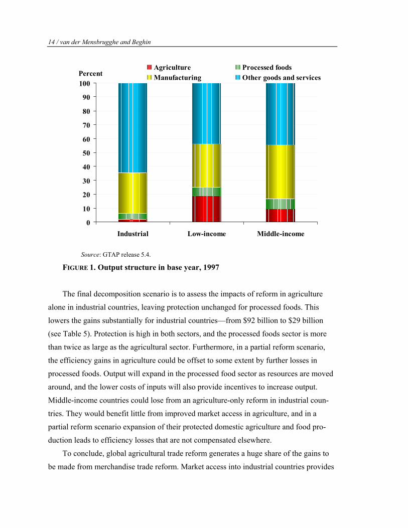
agriculture and food in global output (Figure 1).11 Agriculture represents less than

2 percent of output for industrial countries and 10.5 percent for developing countries,

while processed foods represent 4.5 percent for industrial countries and 7.5 percent for

developing countries. Agriculture is still a relatively high 19 percent of output in the low-

income developing countries. Clearly, protection tends to be higher in agriculture and

food than in other sectors, particularly in industrial countries but in middle-income coun-

tries as well. Protection is more uniform in low-income countries.

For low-income countries the gains from global free trade in agriculture and food

amount to around one-third of the gains from global free trade in all merchandise. This is

a consequence of their dependence on imports of the most protected food items—such as

grains—while they are net exporters of commodities with little or no protection. The

middle-income countries gain 71 percent from global free trade in agriculture and food,

nearly as much as industrial countries, which gain 72 percent as compared with full mer-

chandise trade reform

If reforms are limited to high-income countries—a super version of special and dif-

ferential treatment—with perhaps an agreement by middle-income countries to bind at

existing levels of protection, global gains drop to $102 billion, indicating that a signifi-

cant portion of the global gains is generated by removal of agricultural barriers in

developing countries (see Table 5).12 The drop in gains is particularly striking for mid-

dle-income countries, where the gains from their own agricultural and food reform

would be quite substantial. On a percentage basis, this is less so for low-income coun-

tries. The industrial countries reap gains of $92 billion, implying that agricultural

reform in developing countries could generate gains of about $45 billion for the indus-

trial countries.

TABLE 5. Real income gains from agricultural and food trade reform: Change from 2015 baseline (billion 1997 US$)

Global Merchandise

Trade Reforms Agricultural and Food

Trade Reform Agricultural Trade

Reform Only

Global Global High-Income

Countries High-Income

Countries High-income countries 188.3 136.6 92.0 29.3 Low-income countries 31.9 10.3 3.0 1.1 Middle-income countries 164.7 118.2 6.9 -4.9 Low-income countries, excluding India 19.9 8.4 3.6 1.6 Middle-income countries, including India 176.7 120.1 6.4 -5.3 Developing countries 196.5 128.6 10.0 -3.8 World total 384.8 265.2 102.0 25.5 Source: World Bank simulations with LINKAGE model, based on release 5.4 of the GTAP data.





0

10

20

30

40

50

60

70

80

90

100

Industrial Low-income Middle-income

Agriculture Processed foodsManufacturing Other goods and servicesPercent

Source: GTAP release 5.4. FIGURE 1. Output structure in base year, 1997

The final decomposition scenario is to assess the impacts of reform in agriculture

alone in industrial countries, leaving protection unchanged for processed foods. This

lowers the gains substantially for industrial countries—from $92 billion to $29 billion

(see Table 5). Protection is high in both sectors, and the processed foods sector is more

than twice as large as the agricultural sector. Furthermore, in a partial reform scenario,

the efficiency gains in agriculture could be offset to some extent by further losses in

processed foods. Output will expand in the processed food sector as resources are moved

around, and the lower costs of inputs will also provide incentives to increase output.

Middle-income countries could lose from an agriculture-only reform in industrial coun-

tries. They would benefit little from improved market access in agriculture, and in a

partial reform scenario expansion of their protected domestic agriculture and food pro-

duction leads to efficiency losses that are not compensated elsewhere.

To conclude, global agricultural trade reform generates a huge share of the gains to

be made from merchandise trade reform. Market access into industrial countries provides


significant gains, but a greater share of the gains for developing countries comes from

agricultural trade reform among developing countries. Finally, reform in agriculture alone

provides few benefits. It needs to be linked to reform in the processed food sectors.

Structural Implications. Accelerating integration is one of the key goals of trade re-

form. Beyond the efficiency gains that come from allocating resources to their best uses,

integration is expected to bring productivity increases—scale economies, greater com-

petitiveness, ability to import technology-laden intermediate goods and capital, greater

market awareness, and access to networks.

The potential changes in trade from global reform of agriculture and food are large.

World trade in these two sectors could jump by more than a half a trillion dollars in 2015

(compared with the baseline), an increase of 74 percent (Table 6). Exports in agriculture

and food from developing countries would jump $300 billion, an increase of over

115 percent, with industrial country exports increasing $220 billion, or 50 percent. On the

flip side, imports from both industrial and developing countries would rise substantially.

The net trade position of industrial countries would deteriorate marginally—from

$50 billion in the baseline in 2015 to $48 billion after global reform of agriculture and

food. The marginal improvement for developing countries decomposes into a boost of

nearly $12 billion for low-income countries and deterioration for middle-income coun-

tries of nearly $10 billion.

If the reform is limited to industrial countries, the picture is modified significantly.

First, the change in imports for industrial countries is almost identical under the two

scenarios—$223 billion with full reform and $205 billion with industrial country re-

form only (see Table 6). Developing countries see a significant rise in exports but to

industrial countries only, with little or no change in their own imports. Thus, industrial

countries would witness a much sharper deterioration in their net food bill, with net im-

ports registering a change of $142 billion instead of $2 billion, as under the global

reform scenario. The United States and Europe bear the brunt of the adjustment, with

Canada, Australia, and New Zealand seeing little difference between the global and par-

tial reform scenarios. In other words, these three countries reap much of the trade

benefits from greater market access within industrial countries. Opening up of markets

in developing countries significantly dampens the adjustment process for the United

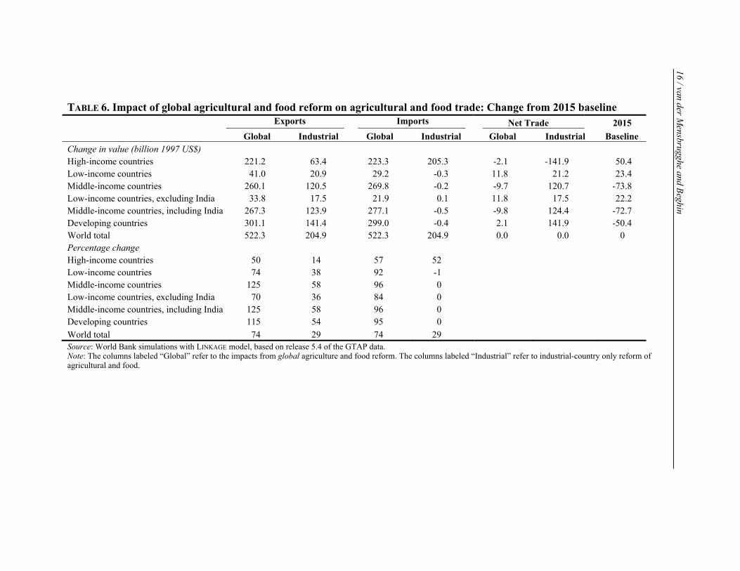
TABLE 6. Impact of global agricultural and food reform on agricultural and food trade: Change from 2015 baseline Exports Imports Net Trade 2015 Global Industrial Global Industrial Global Industrial Baseline Change in value (billion 1997 US$) High-income countries 221.2 63.4 223.3 205.3 -2.1 -141.9 50.4 Low-income countries 41.0 20.9 29.2 -0.3 11.8 21.2 23.4 Middle-income countries 260.1 120.5 269.8 -0.2 -9.7 120.7 -73.8 Low-income countries, excluding India 33.8 17.5 21.9 0.1 11.8 17.5 22.2 Middle-income countries, including India 267.3 123.9 277.1 -0.5 -9.8 124.4 -72.7 Developing countries 301.1 141.4 299.0 -0.4 2.1 141.9 -50.4 World total 522.3 204.9 522.3 204.9 0.0 0.0 0 Percentage change High-income countries 50 14 57 52 Low-income countries 74 38 92 -1 Middle-income countries 125 58 96 0 Low-income countries, excluding India 70 36 84 0 Middle-income countries, including India 125 58 96 0 Developing countries 115 54 95 0 World total 74 29 74 29 Source: World Bank simulations with LINKAGE model, based on release 5.4 of the GTAP data. Note: The columns labeled “Global” refer to the impacts from global agriculture and food reform. The columns labeled “Industrial” refer to industrial-country only reform of agricultural and food.



States and Europe, and the United States would reinforce its net exporting status sig-

nificantly under a global reform scenario.

Most developing countries see a greater improvement in their net food trade with in-

dustrial-country-only reform than with global reform. However, Argentina, Brazil, and

the rest of East Asia improve their net food trade more with global reform than with par-

tial reform. They would gain additional market access from developing countries and

reinforce their comparative advantage over more highly protected countries in East Asia.

The biggest beneficiary on net terms would be China. While its (small) exports would not

change much, removal of its own protection would induce a huge shift in imports. The

lack of reform under the partial reform scenario means that instead of its net food posi-

tion deteriorating by $74 billion in the global reform scenario, it sees a small

improvement of $6 billion. Taken together for developing countries, the partial reform

would generate an improvement in net trade of food of $142 billion.

The structural impacts previously described are associated with global changes in the

distribution of farm income. With global agriculture and food reform, farm incomes

barely change at the global level (a loss of perhaps $10 billion13 or 0.6 percent of baseline

2015 farm income). Changes are much more significant at the regional level (Figures 2

and 3). The largest absolute gains in farm income are in the Americas, Australia and New

Zealand, and developing East Asia excluding China. Latin America would receive

40 percent of the total positive gains; Australia, Canada, and New Zealand, 18 percent;

and the United States, 15 percent.

The relative position of regional gainers is somewhat different, however (see Figure

3). Farmers in Australia, Canada, and New Zealand gain the most from global free trade

in agriculture and food, with income gains of 50–65 percent. Farmers in a number of de-

veloping regions have gains of more than 25 percent, including Vietnam, Argentina,

countries of the Southern Africa Customs Union (SACU), the rest of East Asia (which

includes Thailand, Malaysia, and the Philippines), and the rest of Latin America.

The farmers who lose most are in China, with potential losses of $75 billion in 2015

compared with the baseline scenario.14 The next biggest losers are farmers in Western

Europe and the developed East Asian economies—Japan; the Republic of Korea; and

Taiwan, China. In percentage terms, the biggest losses occur in Japan (30 percent) and


FIGURE 2. Change in rural value added from baseline in 2015 (billion 1997 US$)

FIGURE 3. Percentage change in rural value added from baseline in 2015


Western Europe (24 percent), with China’s losses down to about 15 percent because of its

huge rural economy.

Most of the impact on rural incomes is generated by volume changes, not factor re-

turns. Both labor and capital returns are determined essentially on national markets.15

Thus, wage changes are modest overall, with generally greater impacts in developing

countries, where more labor is employed in agriculture (Table 7). For example, unskilled

wages increase 8 percent in Argentina and Vietnam, and 5–6 percent in the rest of Latin

America and the rest of sub-Saharan Africa. Unskilled workers in Australia and New

Zealand also benefit from these reforms. Unskilled workers in developing countries gen-

erally do better in relative terms than do skilled workers, largely as a result of their

concentration in agricultural sectors. China is a significant exception. Removal of its ag-

ricultural protection lowers demand for unskilled workers, and their wages decline. The

impact on wages in the European Union and Japan is negligible, as agriculture employs a

very small share of the national labor force.

As in the labor markets, the returns in capital market are determined mainly at the

national level (Table 8). Thus, changes to income will largely be reflected in volume

changes, not in price changes. However, direct payments to farmers are implemented as

an ad valorem subsidy on capital (and land), thus creating a wedge between the cost to

farmers and the returns to owners. Removal of the capital subsidy has little effect on

owners since the return is determined at the economywide level, but it raises the costs to

farmers. For example, the cost of capital net of subsidies increases by almost 1 percent in

the European Union, but the average cost to farmers increases by 22 percent—and even

more for livestock producers (43 percent). Note that these capital subsidies are used

mainly in industrial countries, so for most developing countries there is no difference be-

tween the owner return and the cost to farmers.

The changes in the contribution of land to agricultural incomes are driven largely by

price movements—contrary to the case for labor and capital income (Table 9). Land is

essentially a fixed factor in agriculture, with some allowance for movements up and

down the supply curve and for cross-sectoral shifts in land usage.16 In Europe, the aver-

age return to land drops 66 percent, with the supply of land falling 9 percent. Farmers

gain some benefit in lower unit costs because of falling land prices. But removal of the

TABLE 7. Impact of global agriculture and food reform on agricultural employment and wages: Change from 2015 baseline (percent) Total Agriculture Cereals and Sugar Livestock and Dairy Wages Wages Wages

Employ-

ment Unskilled Skilled Employ-

ment Unskilled Skilled Employ-

ment Unskilled Skilled Canada 8.5 1.0 0.8 30.4 1.0 0.8 -15.5 1.0 0.8 United States 0.4 0.6 0.6 -12.4 0.6 0.6 3.3 0.6 0.6 European Union with EFTA -23.7 -0.6 0.4 -57.7 -0.6 0.4 -28.0 -0.6 0.4 Australia and New Zealand 18.2 3.4 2.3 25.6 3.4 2.3 31.1 3.4 2.3 Japan -26.8 -0.9 -0.1 -28.9 -0.9 -0.1 -46.2 -0.9 -0.1 Korea, Rep., and Taiwan, China -13.8 -0.2 0.7 -3.9 -0.2 0.7 8.2 -0.2 0.7 Hong Kong (China) and Singapore 8.8 1.0 0.8 28.8 1.0 0.8 -2.0 1.0 0.8 Argentina 13.3 7.9 5.5 25.8 7.9 5.5 14.3 7.9 5.5 Brazil 12.5 3.4 3.0 25.8 3.4 3.0 11.7 3.4 3.0 China -6.6 -3.1 0.0 -26.6 -3.1 0.0 8.6 -3.1 0.0 India -0.3 0.0 0.2 0.7 0.0 0.2 1.1 0.0 0.2 Indonesia 4.3 1.4 -0.3 6.1 1.4 -0.3 -2.0 1.4 Mexico 5.0 1.3 -0.2 1.3 1.3 -0.2 -4.8 1.3 -0.2 SACU 13.8 1.3 1.1 31.7 1.3 1.1 8.8 1.3 1.1 Turkey 5.2 3.0 0.5 -15.3 3.0 0.5 -18.7 3.0 0.5 Vietnam 17.0 7.8 3.0 63.1 7.8 3.0 -15.4 7.8 3.0 Rest of East Asia 11.6 2.7 0.9 72.0 2.7 0.9 -9.1 2.7 0.9 Rest of South Asia -1.3 -0.2 0.0 1.1 -0.2 0.0 0.7 -0.2 0.0 EU accession countries 6.9 1.6 0.9 12.8 1.6 0.9 13.3 1.6 0.9 Rest of Europe and Central Asia -0.4 -1.0 -0.3 0.3 -1.0 -0.3 -2.4 -1.0 -0.3 Rest of sub-Saharan Africa 6.2 6.0 1.9 17.9 6.0 1.9 1.2 6.0 1.9 Rest of Latin America 6.2 5.4 3.4 17.9 5.4 3.4 42.6 5.4 3.4 Rest of the World including Middle East and North Africa -0.1 -0.3 0.9 2.6 -0.3 0.9 -4.2 -0.3 0.9 Source: World Bank simulations with LINKAGE model, based on release 5.4 of the GTAP data.


TABLE 8. Impact of global agricultural and food trade reform on agricultural capital: Change from 2015 baseline (percent) Total Agriculture Grains and Sugar Livestock and Dairy

Volume Owners’ Return

Farmers’ Cost Volume

Owners’ Return

Farmers’ Cost Volume

Owners’ Return

Farmers’ Cost

Canada -4.9 -0.5 4.1 7.2 -0.5 3.1 -17.0 -0.5 7.1 United States 0.8 0.7 2.6 -19.2 0.7 2.6 4.5 0.7 6.5 European Union with EFTA -32.9 0.7 21.8 -67.1 0.7 21.7 -29.2 0.8 43.1 Australia and New Zealand 40.2 0.6 1.2 3.0 0.7 1.3 123.5 0.6 1.7 Japan -22.9 1.7 4.9 -25.0 1.7 7.6 -47.0 1.7 12.2 Korea, Rep., and Taiwan, China -4.3 0.7 12.0 8.9 0.8 15.4 17.5 0.8 103.8 Hong Kong (China) and Singapore 9.8 0.7 0.7 75.4 0.7 0.7 -4.3 0.7 0.7 Argentina 6.0 4.2 4.2 9.0 4.2 4.2 17.9 4.2 4.2 Brazil 10.1 3.1 3.1 21.9 3.1 3.1 9.8 3.1 3.1 China -2.7 3.2 3.2 -17.5 3.2 3.2 5.8 3.2 3.2 India 0.0 0.1 0.1 0.8 0.1 0.1 1.2 0.1 0.1 Indonesia 0.7 -0.2 -0.2 1.0 -0.2 -0.2 -0.9 -0.2 -0.2 Mexico 4.3 -0.1 3.7 2.3 -0.1 4.4 -7.5 -0.1 9.1 SACU 19.5 -0.6 -0.6 39.4 -0.6 -0.6 25.4 -0.6 -0.6 Turkey 0.2 -0.4 -0.2 -15.8 -0.4 0.5 -15.1 -0.4 -0.4 Vietnam 2.4 1.8 1.8 28.7 1.8 1.8 -13.3 1.8 1.8 Rest of East Asia 20.9 0.2 0.2 36.5 0.2 0.2 -8.6 0.2 0.2 Rest of South Asia 0.1 1.3 1.3 2.3 1.3 1.3 0.7 1.2 1.2 EU accession countries -0.2 0.5 21.6 7.7 0.5 18.9 -6.3 0.5 67.6 Rest of Europe and Central Asia -2.5 1.6 7.7 -1.9 1.6 8.3 -5.8 1.6 9.3 Rest of sub-Saharan Africa 0.5 –1.1 –1.1 5.6 –1.1 –1.1 4.0 –1.1 –1.1 Rest of Latin America 6.2 1.8 1.8 15.9 1.8 1.8 41.1 1.8 1.8 Rest of the World including Middle East and North Africa 0.3 –0.2 –0.2 2.9 –0.2 –0.2 –3.7 –0.2 –0.2

Source: World Bank simulations with LINKAGE model, based on release 5.4 of the GTAP data.




TABLE 9. Impact of global agriculture and food reform on agricultural land: Change from 2015 baseline (percent) Total Agriculture Cereals and Sugar Livestock and Dairy

Price Price Price Land Owner Farmer Land Owner Farmer Land Owner FarmerCanada -6.4 69.5 133.8 6.6 76.9 192.8 -25.2 56.8 83.5 United States 2.4 -5.1 22.1 -19.0 -12.5 42.1 12.3 -0.2 9.1 European Union with EFTA -9.4 -66.3 -57.0 -58.9 -74.1 -4.7 -3.5 -65.0 -59.7 Australia and New Zealand 6.2 197.8 219.1 1.9 197.0 224.0 34.8 219.6 252.4 Japan -21.0 -44.9 -41.5 -24.0 -45.5 -34.6 -34.1 -48.9 -48.9 Korea, Rep., and Taiwan, China -11.4 -27.6 -27.1 -0.2 -25.3 -24.6 4.1 -23.0 -20.9 Hong Kong (China) and Singapore 11.1 64.2 64.2 -22.0 45.0 45.0 -2.3 58.0 58.0 Argentina 4.5 56.2 56.2 11.4 59.5 59.5 12.0 60.0 60.0 Brazil 9.9 18.0 18.0 23.8 22.9 22.9 8.6 17.6 17.6 China -0.9 -25.7 -25.7 -21.1 -31.1 -31.1 7.6 -23.6 -23.6 India 0.0 -1.8 -1.8 0.8 -1.5 -1.5 1.4 -1.3 -1.3 Indonesia 0.7 10.9 10.9 2.1 11.4 11.4 -1.8 10.0 10.0 Mexico 2.7 0.6 13.1 -8.9 -3.6 52.1 -1.6 -0.6 0.8 Southern African Customs Union 8.0 86.4 86.4 26.4 95.2 95.2 4.5 84.9 84.9 Turkey 0.8 47.3 47.3 -14.9 39.0 39.0 -20.2 36.1 36.1 Vietnam -0.3 44.6 44.6 33.2 60.3 60.3 -16.0 38.1 38.1 Rest of East Asia -1.5 34.1 34.1 43.7 53.8 53.8 -9.6 32.7 32.7 Rest of South Asia -0.1 -6.0 -6.0 3.2 -5.0 -5.0 1.3 -5.4 -5.4 EU accession countries 2.6 2.0 6.1 4.6 2.8 10.8 7.5 3.5 8.8 Rest of Europe and Central Asia -1.5 -2.4 -2.4 -1.1 -2.3 -2.3 -1.2 -2.2 -2.2 Rest of sub-Saharan Africa -0.3 62.8 62.8 9.0 67.9 67.9 -2.4 61.7 61.7 Rest of Latin America 1.0 55.4 55.4 5.0 58.6 58.6 40.3 74.9 74.9 Rest of the World including Middle East and North Africa 0.0 0.1 0.1 2.7 0.8 0.8 -4.3 -1.2 -1.2 Source: World Bank simulations with LINKAGE model, based on release 5.4 of the GTAP data.



direct subsidy does not allow farmers to reap the full cost gains from falling land prices.

The average cost for farmers drops 57 percent, lower than the drop in the rental price of

land (66 percent). And the change in the cost structure is highly sector specific. Thus, ce-

real and grain farmers see a small drop in their net cost of land (5 percent); however, the

drop in the price of land does not compensate for removal of the subsidies since the re-

turns to owners fall by 74 percent. This is not the case in the livestock sector, where

subsidy payments are linked to capital (the herds) and not to land. The impacts in the

United States are muted, with the overall return to landowners changing slightly—a de-

cline of 5 percent—but costs to farmers increasing substantially—22 percent on average

and more than 42 percent for cereal and sugar producers.

In most developing countries, land prices increase substantially, except in China and

in a few other regions. This may reduce to some extent the positive distributional impacts

from relatively higher wages for unskilled labor since land ownership may not necessar-

ily be congruent with the unskilled labor working the land. There are some interesting

sectoral shifts. For example, China would see more land devoted to livestock and dairy,

and less to cereals, which would be imported from lower-cost sources.

Sensitivity Analysis This section uses sensitivity analysis to explore how results change when some of the

basic assumptions of the model change. It focuses on four areas:

• The agricultural productivity assumptions of the standard baseline scenario. Agri-

cultural productivity is cut by 1 percentage point in developing countries and the

results from global agriculture and food reform are compared with the results us-

ing the default productivity assumptions. In a separate analysis, productivity is

increased for middle-income developing countries.

• The impacts of the mobility of agricultural capital. Agricultural capital is more

closely tied to the sector, making it more difficult to shed and leading to a different

transition when reform is undertaken.

• Sensitivity of the results to supply rigidities in developing countries.

• Sensitivity of the results to the key trade elasticities.


Agricultural Productivity Agricultural productivity is assumed to grow 2.5 percent a year globally in the stan-

dard baseline scenario based on existing evidence (Martin and Mitra 1996, 1999). This

may be too optimistic for developing countries, particularly for low-income countries.

This assumption may have an impact on long-term self-sufficiency rates, particularly of

sensitive commodities. The more that trade reform raises the world price of food, the

more net food importers will be adversely affected by negative terms-of-trade shocks. To

test the sensitivity of the trade results to agricultural productivity, a different baseline was

construed with agricultural productivity improving at a slower 1.5 percent for developing

countries but remaining at 2.5 percent for industrial countries.

Trade Impact. Under the standard baseline, high-income countries go from a position

of net food importers in 1997 to net food exporters in 2015 (Table 10). Low-income

countries improve their position significantly, going from a positive food balance of

$12.5 billion in 1997 to $23 billion in 2015. The position of middle-income countries de-

teriorates, however. Under the low-productivity baseline, the net food trade position of

industrial countries increases substantially—jumping to $151 billion in 2015 compared

with only $50 billion in the standard baseline. Low-income countries still maintain a

positive balance but one that is much closer to zero than in the previous baseline. And the

net food trade situation of middle-income countries shows a greater dependence on world

markets.

Whereas reform in the standard baseline positions low-income countries as net food

exporters and has only a mild negative effect on the food balance of high- and middle-

income countries, under the low-productivity assumption the food trade balance of the

high-income countries improves substantially—by $30 billion—largely because of an

increased dependence on food imports by middle-income countries. The low-income

countries still see an improvement in their trade balance but by a more modest

$3.6 billion rather than the nearly $12 billion using the standard productivity assump-

tions.

Output Impact. Average annual agricultural output growth in developing countries

slows from 3.3 percent in the standard baseline to 2.6 percent in the low-productivity

baseline (Table 11). In industrial countries, higher productivity provides an opportunity

TABLE 10. Net trade impacts assuming lower agricultural productivity in developing countries (billion 1997 US$) Standard Productivity Low Productivity Baseline Reform Baseline Reform 1997 2015 2015 2015 2015 High-income countries -23.1 50.4 48.4 151.2 181.6 Low-income countries 12.5 23.4 35.2 0.9 4.5 Middle-income countries 10.5 -73.8 -83.6 -152.0 -186.1 Low-income countries, excluding India 7.4 22.2 34.1 8.5 17.2 Middle-income countries, including India 15.6 -72.7 -82.4 -159.7 -198.9 Developing countries 23.1 -50.4 -48.4 -151.2 -181.6 Source: World Bank simulations with LINKAGE model, based on release 5.4 of the GTAP data.

TABLE 11. Impacts on output assuming lower agricultural productivity for developing countries

Growth in 2000–15

(percent) Baseline Difference

in 2015 Difference Between Baseline and Reform

Scenario in 2015

Low

Baseline Standard Baseline

Value (billion $)

Percentage Change

Low (billion $)

Standard (billion $)

Low (percent)

Standard (percent)

High-income countries 1.9 1.2 122.6 12.4 -100.0 -107.7 -9.0 -10.9 Low-income countries 2.8 3.6 -71.6 -11.4 8.7 12.1 1.6 1.9 Middle-income countries 2.6 3.2 -166.2 -9.4 27.0 37.2 1.7 2.1 Low-income countries, excluding

India 3.0 3.7 -39.4 -11.6 10.3 12.3 3.4 3.6 Middle-income countries,

including India 2.6 3.2 -198.4 -9.7 25.4 37.0 1.4 1.8 Developing countries 2.6 3.3 -237.8 -10.0 35.7 49.4 1.7 2.1 World total 2.4 2.6 -115.2 -3.4 -64.3 -58.3 -2.0 -1.7 Source: World Bank simulations with LINKAGE model, based on release 5.4 of the GTAP data.





to gain market share, and higher world prices relative to the original baseline provide

greater incentives to produce. World output under the alternative scenario declines

3.4 percent (higher prices lead to reduced demand), with a reallocation between industrial

and developing countries. Industrial countries benefit from a 12 percent increase in out-

put in 2015 compared with the standard baseline, whereas developing-country output is

reduced by some 10 percent.

With respect to output impacts following the trade reform scenario, the qualitative

results of the different baseline assumptions of agricultural productivity are identical—

trade reform of agriculture and food lead to a shift in agricultural production from indus-

trial to developing countries. In the standard baseline, developing-country agricultural

output increases more than 2 percent, whereas in the low-productivity baseline the in-

crease is only 1.7 percent. The decline in industrial countries drops to 9 percent, from

11 percent in the standard baseline. The changes in output patterns across regions are

identical, though the magnitudes differ.

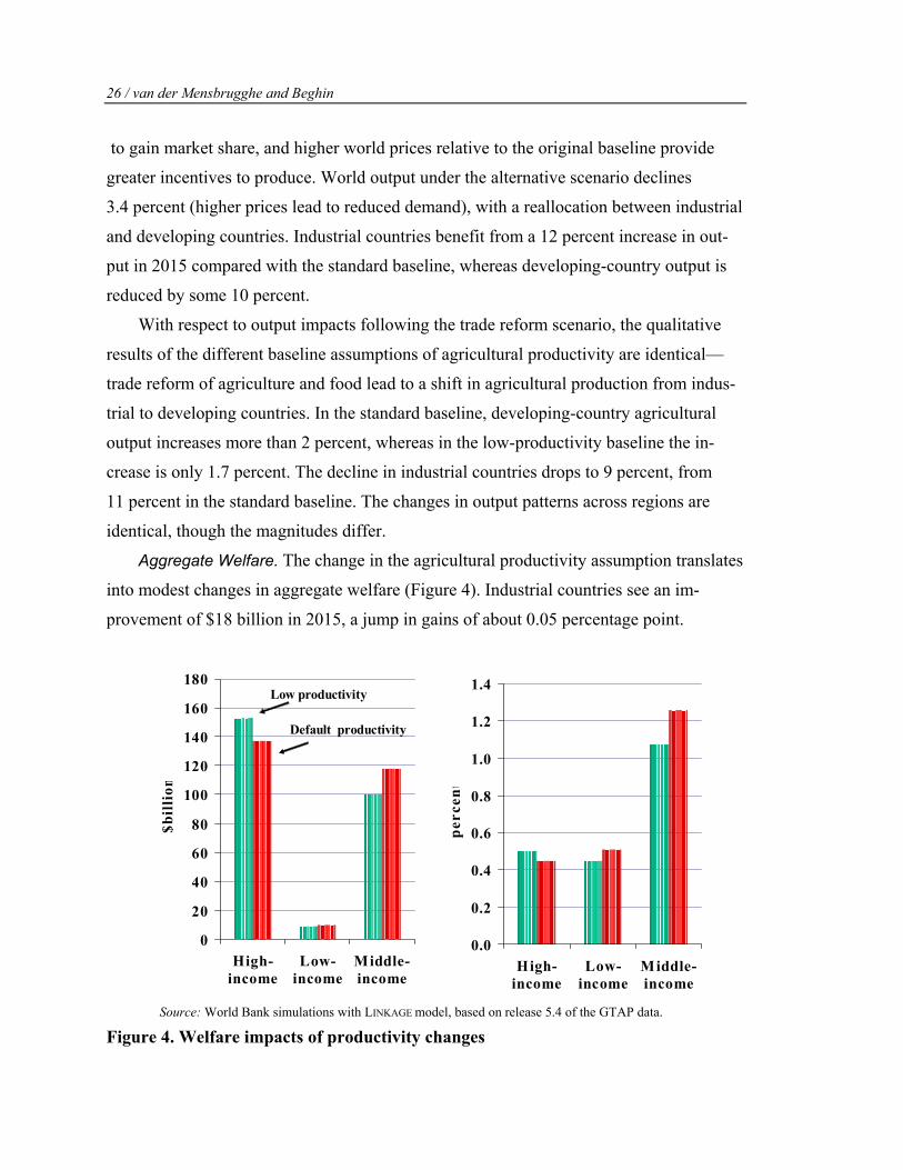
Aggregate Welfare. The change in the agricultural productivity assumption translates

into modest changes in aggregate welfare (Figure 4). Industrial countries see an im-

provement of $18 billion in 2015, a jump in gains of about 0.05 percentage point.

0

20

40

60

80

100

120

140

160

180

High-income

Low-income

Middle-income

$bil

lion

Low productivity

Default productivity

0.0

0.2

0.4

0.6

0.8

1.0

1.2

1.4

High-income

Low-income

Middle-income

perc

ent


Figure 4. Welfare impacts of productivity changes


Developing countries see a reduction in their welfare gains, with low-income countries

seeing a drop of $1.4 billion (0.08 percentage point) and middle-income countries a drop

of $17.8 billion (0.19 percentage point).

A High Productivity Assumption. Many middle-income countries such as Argentina,

Brazil, and Thailand have experienced rapid growth in agriculture, suggesting the poten-

tial for higher productivity growth than assumed in the standard baseline. To explore this,

agricultural productivity growth was raised from 2.5 percent to 4.0 percent for middle-

income countries (China, India, Indonesia, rest of East Asia, Vietnam, Argentina, Brazil,

Mexico, rest of Latin America, the EU accession countries, rest of Europe and Central

Asia, and Turkey).

Changes are as expected. Agricultural supply and exports expand for natural export-

ers such as Argentina and Brazil. China, the largest middle-income importer, reduces its

deficit by about $18 billion (Table 12). The middle-income group, including India, ex-

periences a net surplus of $30 billion in 2015, whereas under the standard baseline it has

a deficit of $19 billion. High-income countries experience a deterioration of their net ag-

ricultural trade of about $50 billion, compared with $3 billion in the standard baseline,

and Europe’s deficit increases to nearly $60 billion. Results for the food sector are quali-

tatively similar but smaller in size, with an increase in competitiveness of food processing

in middle-income countries and a decrease in net trade by high-income countries relative

to the standard baseline (Table 13). These large changes show how sensitive baseline tra-

jectories are to changes in assumptions about the future. They do not, however, affect the

impact of the reform scenario measured in deviations from the baseline.

In conclusion, the baseline assumptions regarding productivity are important, though

changes in the assumption would not yield substantially different results from agriculture

and food trade reform for developing countries in terms of net benefits and agricultural

output.17 However, lower productivity would reduce the level of food self-sufficiency

among developing countries—particularly middle-income countries—and could lead to a

different assessment of the direction of food self-sufficiency in the aftermath of reform.

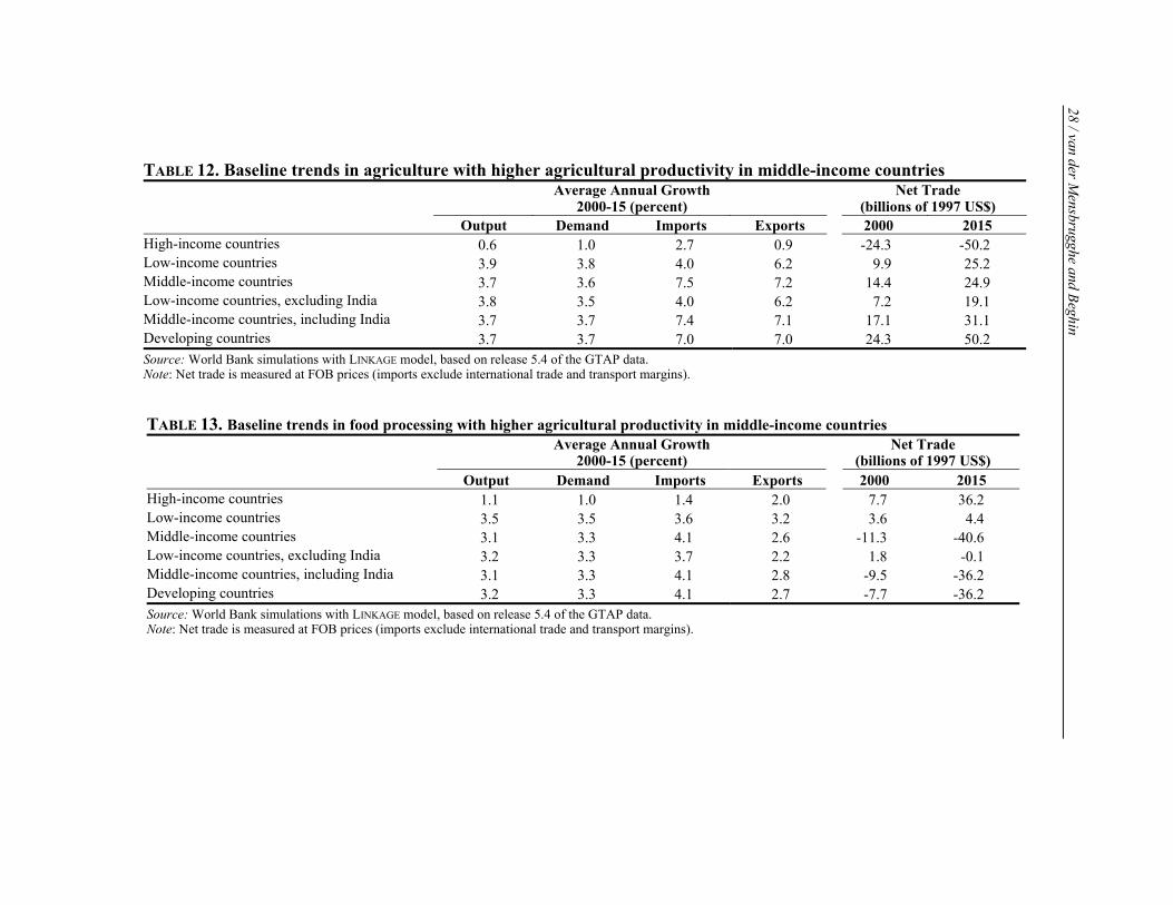
TABLE 12. Baseline trends in agriculture with higher agricultural productivity in middle-income countries

Average Annual Growth

2000-15 (percent) Net Trade

(billions of 1997 US$) Output Demand Imports Exports 2000 2015

High-income countries 0.6 1.0 2.7 0.9 -24.3 -50.2 Low-income countries 3.9 3.8 4.0 6.2 9.9 25.2 Middle-income countries 3.7 3.6 7.5 7.2 14.4 24.9 Low-income countries, excluding India 3.8 3.5 4.0 6.2 7.2 19.1 Middle-income countries, including India 3.7 3.7 7.4 7.1 17.1 31.1 Developing countries 3.7 3.7 7.0 7.0 24.3 50.2 Source: World Bank simulations with LINKAGE model, based on release 5.4 of the GTAP data. Note: Net trade is measured at FOB prices (imports exclude international trade and transport margins).

TABLE 13. Baseline trends in food processing with higher agricultural productivity in middle-income countries

Average Annual Growth

2000-15 (percent) Net Trade

(billions of 1997 US$) Output Demand Imports Exports 2000 2015

High-income countries 1.1 1.0 1.4 2.0 7.7 36.2 Low-income countries 3.5 3.5 3.6 3.2 3.6 4.4 Middle-income countries 3.1 3.3 4.1 2.6 -11.3 -40.6 Low-income countries, excluding India 3.2 3.3 3.7 2.2 1.8 -0.1 Middle-income countries, including India 3.1 3.3 4.1 2.8 -9.5 -36.2 Developing countries 3.2 3.3 4.1 2.7 -7.7 -36.2 Source: World Bank simulations with LINKAGE model, based on release 5.4 of the GTAP data. Note: Net trade is measured at FOB prices (imports exclude international trade and transport margins).



Mobility of Agricultural Capital and the Transition in Industrial Countries The focus so far has been mainly on the long-term impact of the removal of protec-

tion, with little attention to the transitional impacts. A key mechanism of the model is the

vintage structure of capital. Sectors in decline have excess capital that will not readily be

used in other sectors. This is certainly the case with agricultural capital, although some

could be used for nonagricultural purposes and other equipment could be used in nonpro-

tected agricultural sectors.

Excess capital is released to other sectors following an upward-sloping supply curve.

The value for the supply elasticity in the standard model is 4. To test the importance of

this elasticity, the reform scenario is simulated again but with a supply elasticity of 0.5.

This makes excess supply much less mobile and, all else equal, will tend to increase sup-

ply relative to the same simulation with a higher supply elasticity.

Consider the case for the sugar sector in Europe. The starting point is 2004, since the

trade reform starts in 2005. Under the baseline, sugar output in Europe increases mod-

estly between 2004 and 2015 (Figure 5). With the start of reform, output drops rapidly,

0

5

10

15

20

25

30

35

40

45

2004 2005 2006 2007 2008 2009 2010 2011 2012 2013 2014 2015

$billion

Baseline

Standard supply elasticity

Low supply elasticity


FIGURE 5. Sugar output in Europe (billion US$)


and by 2015 output has fallen from about $42 billion to about $11 billion. The supply

elasticity has an impact on the rate of decline of sugar output, but the final level is

identical. Thus, with a low supply elasticity, the transition is drawn out over a longer pe-

riod. The rate of decline between 2004 and 2010 is 18.4 percent using the standard

elasticity and 16.5 percent with the lower elasticity.

There are only a handful of sectors in industrial countries in which the supply elastic-

ity has any noticeable impact: wheat and sugar in the United States; rice, wheat, other

grains, oil seeds, and sugar in the European Union; and wheat and oil seeds in Japan. The

aggregate impacts on agricultural production are negligible, at less than 1 percent over all

industrial countries in any given year, and at most 0.3 percent for developing countries,

but in the opposite direction. There are no discernible impacts on welfare.

In conclusion, lowering the supply elasticity will draw out the supply response dur-

ing the transition phase but will have no discernible long-term impact on the results.

Supply Response in the Low-Income Countries This section evaluates the impact of lowering the land supply response in three re-

gions—the rest of South Asia, the SACU region, and the rest of sub-Saharan Africa—to

examine whether low-income countries, with their potentially low supply response, will

benefit from greater market access. This involves three parameters. First, the base-year

land supply elasticity was reduced from 1 to 0.25. Second, the land supply asymptote was

reduced from 20 percent of the initial land supply to 10 percent.18 These two parameters

determine aggregate land supply. A third parameter moderates the degree of land mobil-

ity across sectors. The allocation of land across sectors is governed by a constant

elasticity of transformation function.19 The standard transformation elasticity is 3, a rela-

tively elastic value. In the sensitivity simulation, the transformation elasticity for the three

regions is set to 0.5.

The lower land supply elasticities affect the baseline scenario. For the three regions

where changes were made to supply elasticities, the overall rate of growth of agricultural

output between 2000 and 2015 declines from 3.4 to 3.1 percent in the rest of South Asia

and from 4.0 to 3.8 percent in rest of sub-Saharan Africa; it remains the same for SACU

at 2.1 percent (Table 14). In all three regions, the most affected crop is plant-based fibers.

These three regions have a sizable market share at the global level in 1997 of 1.4 percent


TABLE 14. Impact of lower land supply elasticities in rest of South Asia and sub-Saharan Africa (percent) Baseline Growth Rates 2000–15 Impact of Trade Reform

Standard Supply

Elasticity

Low Supply

Elasticity

Baseline Difference

in 2015

Standard Supply

Elasticity

Low Supply

Elasticity Rest of South Asia Rice 2.8 2.7 -2.1 3.4 2.4 Wheat 2.7 2.6 -3.8 34.4 19.6 Other grains 3.8 3.6 -3.6 -2.4 -1.5 Oil seeds 4.1 3.5 -9.1 -10.0 -6.8 Sugar 3.8 3.3 -8.9 -17.2 -12.4 Plant-based fibers 4.5 3.7 -13.2 19.2 6.2 Other crops 3.6 3.2 -7.3 -8.0 -5.4 Cattle 4.0 3.7 -4.9 1.7 1.5 Other meats 4.1 3.6 -8.3 -1.0 -1.8 Raw milk 3.9 3.5 -6.1 1.3 1.3 Total 3.4 3.1 -5.6 -0.2 -0.6 Southern Africa Customs Union Rice 2.3 2.4 -1.7 8.8 8.4 Wheat 1.9 1.9 -0.5 0.0 0.5 Other grains 1.1 1.3 0.8 29.5 19.9 Oil seeds 1.6 1.8 -1.8 9.2 8.6 Sugar 1.3 1.4 -0.2 87.7 50.6 Plant-based fibers 6.0 3.8 -35.9 3.4 3.6 Other crops 2.4 2.4 -8.7 7.2 4.3 Cattle 2.2 2.2 0.0 24.2 23.0 Other meats 2.2 2.2 0.1 5.0 5.1 Raw milk 2.2 2.2 0.0 -2.7 -2.6 Total 2.1 2.1 -2.9 18.4 14.0 Rest of sub-Saharan Africa Rice 3.2 3.2 -0.1 -1.2 -0.9 Wheat 3.4 3.5 0.4 0.3 3.0 Other grains 3.2 3.2 0.4 -0.1 3.0 Oil seeds 3.9 3.8 -0.8 51.0 37.7 Sugar 3.2 3.2 1.5 48.1 40.3 Plant-based fibers 8.1 6.5 -23.2 42.8 24.9 Other crops 4.5 4.2 -5.8 -3.6 0.0 Cattle 3.5 3.4 -1.4 4.6 3.5 Other meats 3.7 3.6 -1.9 -0.7 0.3 Raw milk 3.3 3.3 -1.1 1.7 1.2 Total 4.0 3.8 -4.1 5.6 4.9 Source: World Bank simulations with LINKAGE model, based on release 5.4 of the GTAP data


for plant-based fibers and 15 percent for rice. However, the demand for rice is much less

elastic than for plant-based fibers. The lower supply elasticity would make land relatively

more costly, all else equal, and given the higher demand elasticities, the higher land

prices will be reflected in lower demand from these three regions.

The impact of trade reform on agricultural output using both the standard and the

lower land elasticities is broadly the same qualitatively though lower in magnitude in

general. Considering again the case of sugar, output increases 88 percent in SACU and

48 percent in the rest of sub-Saharan Africa using the standard supply elasticity. Sugar

output expansion drops to 51 percent in SACU and 40 percent in the rest of sub-Saharan

Africa when lower land supply elasticity is assumed.

The welfare impacts are modest but measurable, and the results reflect only some of

the possible supply constraints in low-income countries. For the three regions under ques-

tion, aggregate welfare would decline $1.1 billion compared with the standard

assumption, and it would drop from 1.2 percent to 1.1 percent of baseline income.

Trade Elasticities The most critical parameter in trade reform scenarios is trade elasticities. There is

ongoing debate about their size. Most econometric evidence suggests that the Armington

elasticities (measuring the degree of substitutability between domestic and imported

goods) are low, in the range of 1 to 2.20 The studies are riddled with data problems, par-

ticularly the evaluation of unit values, and many trade economists downplay the

empirical evidence, for two main reasons. First, low Armington elasticities lead to im-

plausible terms-of-trade effects. And second, low elasticities would suggest high optimal

tariffs. Trade studies fall into three groups: those with relatively low elasticities (1–3),

those with middling elasticities (3–6), and those with very high elasticities (20–40). Ex-

amples of the first are the MONASH model (Dixon and Rimmer 2002) and the standard

GTAP model (Hertel 1996). Recent World Bank work has been using the middling elas-

ticities. High elasticities are mainly associated with the work of Harrison, Rutherford, and

Tarr (see, for example, their 2003 article).

The impacts of the agriculture and food trade reform were reassessed using two al-

ternative elasticities. A low scenario uses trade elasticities 50 percent lower than the

standard, and a high scenario uses trade elasticities 50 percent higher than the standard


(the standard values used in this study are shown in Annex Table A.3, available from the

authors). Each set of assumptions requires two simulation runs. A new baseline is con-

structed each time, with all assumptions identical except for the trade elasticities, and the

reform scenario is simulated. Thus, the comparisons are between each individual baseline

and each associated reform scenario.

Within this range of trade elasticities the model exhibits some modest nonlinearity,

particularly on the upside (Figure 6). For all three regions the 50 percent higher elastic-

ities lead to a greater than 50 percent rise in real income gains—particularly for

developing regions, where the rise is almost 75 percent. On the downside, both high- and

low-income regions see an equiproportionate fall in the real income gains relative to the

elasticities, with a fall to 40 percent of the standard gains in the case of the middle-

income countries. The higher elasticities dampen the adverse terms-of-trade shocks from

reforms, leading to the higher income gains. The global gains vary from a low of

$126 billion to a high of $438 billion, with the gains at $265 billion using the standard

elasticities.

0

25

50

75

100

125

150

175

200

High-income Low-income Middle-income

LO Default HI

Index relative to default elasticities in 2015


FIGURE 6. Real income and trade elasticities


For some countries and regions the range of results is much broader than at the ag-

gregate level. For example, Mexico would lose some $1.2 billion with the low elasticities

and gain $3 billion with the high elasticities compared with a gain of 0.9 with the stan-

dard elasticities. Several other regions show similar variation. The standard deviation of

the index across all developing countries is 130 in the case of the high elasticities,

whereas the weighted average is 170.

The impacts on trade are similar to the impacts on income but exhibit more nonlin-

earity (Figure 7). At the global level, exports increase 80 percent using the high

elasticities and decline 60 percent using the low elasticities (with export increases ranging

from a low of $216 billion to nearly $1 trillion). There is also less variability across re-

gions of the model than with the income results. In isolation, the trade elasticities appear

to have the greatest impact in determining the overall outcomes of trade reform, although

other model changes—both in specification and in elasticities—combined may be at least

as important in determining overall outcomes. This is an area of active research for better

determining the bounds on the possible ranges for these elasticities. Improved data

0

25

50

75

100

125

150

175

200

High-income Low-income Middle-income

LO Default HI

Index relative to default elasticities in 2015


FIGURE 7. Exports and trade elasticities


would help, but there are still issues relating to model specification and aggregation that

need to be thought through.

Conclusions This quantitative assessment of the impact of agricultural and food market distortions

on incomes, welfare, trade, and output shows that the changes in cross-regional patterns

of output and trade tend to be much larger than are the more familiar gains to real in-

come. A decomposition of the aggregate results across policy instruments and regions

shows that reforms in agriculture and food account for a large share of the global gains of

reforms of total merchandise trade. This result is driven by the relatively low protection

levels in manufacturing sectors. Another major finding is that developing countries have

more to gain from reforming their own support policies than from reforms in high-

income countries. Symmetrically, high-income countries would experience larger welfare

gains from their own reforms than from developing countries’ reforms. These dimensions

of the debate are often overlooked but are crucial. Global reform leads to additive results

with aggregate gains close to the gains from reforms in each group. A third key finding is

that agricultural reform alone in high-income countries would create moderate gains,

about 10 times smaller than those of a combined reform of food and agricultural markets.

Developing countries would be negatively affected as a group, because their own distor-

tions would be exacerbated by the agricultural reforms in high-income countries.

The results are broadly robust to changing assumptions on future agricultural produc-

tivity in developing countries, supply constraints, and level of the trade elasticities, but

the levels of the trade elasticities remain of foremost importance. The trade effects of re-

forms are also sensitive to assumptions about agricultural productivity gains in

developing countries. Assuming low-productivity gains leads to a reversal in the esti-

mated impact of global liberalization for industrial countries, increasing their net food

trade surplus, as middle-income countries become much larger importers of food and ag-

ricultural products. Low-income countries experience an increase in net food trade

surplus that is much smaller than under the higher productivity assumption. Hence, varia-

tions in productivity could lead to a different assessment of the direction of food self-

sufficiency after reform. Supply constraints do not qualitatively affect the estimated im-


pact of trade reform on agricultural output, although estimated changes tend to be

smaller. Higher trade elasticities dampen the adverse terms-of-trade shocks from reforms,

leading to higher income gains. The global gains vary from a low of $126 billion with

low elasticities to a high of $438 billion with high elasticities, with the gains at

$265 billion using the standard elasticities. There is also higher variation at the individual

country level.

The changes in agricultural value added and factor prices are considerable in several

cases. The estimated loss of rural value-added is large in Japan and the European Union,

the Republic of Korea, Taiwan (China), and China. Thus, considerable adjustment and

displacement of resources would take place to reflect these changes. Cairns Group coun-

tries and the United States experience sizable gains in rural value-added, as do SACU and

the rest of sub-Saharan Africa. Wages for unskilled labor in developing countries are

moderately influenced by major policy reforms, such as in China, where they decrease,

but more significantly in Argentina, where they increase.

Endnotes

1. The model is based at the World Bank and uses the GTAP release 5.4 dataset (see van der Mensbrugghe 2003 for details).

2. East Asia is divided into four economies: China, Indonesia, Vietnam and the rest. South Asia has two components: India and the rest. Latin America has four econo-mies: Argentina, Brazil, Mexico, and the rest. Europe and Central Asia are split into three components: the European Union accession countries, Turkey, and the rest. Sub-Saharan Africa has two components: the Southern Africa Customs Union (SACU) countries, and the rest. And the Rest of the World region has all other coun-tries including the Middle East and North Africa.

3. See van der Mensbrugghe 2003 for a technical description of the model.

4. Agricultural policies derived from the Agricultural Market Access Database (AMAD) reflect 1998/99 levels of support, except for cotton, for which International Cotton Advisory Committee data were used (see Baffes 2004).

5. Income elasticities are held more or less constant over the time horizon. With China’s rapid growth, one might anticipate a convergence of income elasticities to-ward levels in higher-income countries and thus a dampening of food growth over time relative to incomes.

6. Textile and apparel quotas that generate quota rents for exporters are converted to export taxes (for the country of origin). In the current simulations, these have not been eliminated.

7. Technically, it is a measure of the Hicksian equivalent variation. When comparing aggregate welfare measures across studies, it is important to convert them to similar scales. Thus, $350 billion in 2015 is more or less equivalent to $250 billion in 2004 and $200 billion in 1997, assuming an average annual global GDP growth rate of 3 percent (all in 1997 US$, the base year of release 5 of the GTAP data set). Assum-ing a world inflation rate of 2.5 percent over the entire period, the measured $250 billion in 2004 in 1997 dollars becomes $300 billion in 2004 dollars.

8. The Mercosur preferential agreement is not incorporated in the standard GTAP data-set but is included in the dataset used for these simulations. Efforts were made to minimize distortions to the original social accounting matrix while adjusting the original dataset.


9. There is also an issue regarding whether bound or applied tariffs are liberalized. Most developing countries have bound their tariffs at rates much higher than applied rates. Negotiations concern the bound tariffs; the reforms described here are relative to the applied tariffs. For a full reform scenario, it is not much of an issue, but for analyzing potential outcomes of a negotiation, it could be.

10. See the Global Economic Prospects publications for 2002 and 2004 (World Bank 2001, 2003). The 2002 report notes dynamic gains of $830 billion compared with static gains of $350 billion, with a range of up to $1,340 billion depending on some key parameters (see Table 6.2, page 171).

11. Figure 1 shows output shares in the base year. One would assume that the agricul-tural and food shares are declining over time, as income elasticities for food tend to be lower than for other goods and services.

12. While the model is highly nonlinear, the results to a close approximation are rela-tively additive.

13. Nominal values are measured with respect to the model’s numéraire—the average export price of manufactured exports from industrial countries.

14. This should be considered an upper bound on China’s potential loss since the base-line scenario does not include the impacts of China’s accession to the WTO. Thus, the reform scenario is capturing the combined gains from global reform and China’s WTO accession, which include the gains to be had from reforming from 1998/99 base agricultural policies.

15. Sector-specific capital returns may be possible during the transition phase, as sectors in decline shed unwanted capital. The most mobile equipment will be shed first, and the return to the remaining capital may be priced lower than the national rate of re-turn to capital.

16. In the default version of the model, cross-sectoral transformation elasticities are set to 3. Thus a 10 percent rise in the return in one sector (relative to the others) will lead to a 30 percent shift of land into that sector. Because of the finite transformation elasticity, land prices are sector specific.

17. Given the aggregate nature of the model, the impacts on vulnerable countries or sec-tors are harder to assess. In particular, sub-Saharan Africa is a heterogeneous subcontinent that is not reflected in the level of aggregation of this study.

18. The land supply function is governed by a logistic curve. It is calibrated in the base year to an exogenously given elasticity and the value of the asymptote relative to the base supply level. Thus, if the asymptote is set to 1.2, land supply can increase by at most 20 percent above its base level.

19. The elasticity measures the ease of shifting land from one activity to another when the relative price of these two activities changes.


20. More recent econometric work is resulting in higher estimates for the trade elastic-ities and these are now being reflected in the forthcoming release of the GTAP dataset.

References

Baffes, J. 2004. “Cotton: Market Setting, Trade Policies, and Issues.” Chap. 14 in Global Agricultural Trade and the Developing Countries. Edited by M.A. Aksoy, and J.C. Beghin. Oxford, UK: Oxford University Press and The World Bank, in press.

Beghin J., D. Roland-Holst, and D. van der Mensbrugghe. 2003. “How Will Agricultural Trade Reforms in High-Income Countries Affect the Trading Relationships of Developing Countries?” In Agriculture, Trade, and Poverty: Making Policy Analysis Count. Paris: OECD Publications.

Dixon, P.B., and M.T. Rimmer. 2002. Dynamic, General Equilibrium Modelling for Forecasting and Pol-icy: A Practical Guide and Documentation of MONASH. Boston: North-Holland.

Harrison, G.W., T.F. Rutherford, and D. Tarr. 2003. “Trade Liberalization, Poverty and Efficient Equity.” Journal of Development Economics 71(1): 97–128.

Hertel, T.W. 1996. Global Trade Analysis: Modeling and Applications. Cambridge: Cambridge University Press.

Martin, W., and D. Mitra. 1996. “Productivity Growth in Agriculture and Manufacturing.” International Economics Department, World Bank, Washington, DC.

———. 1999. “Productivity Growth and Convergence in Agriculture and Manufacturing.” Working Pa-pers, Agriculture: Land, Commodity Prices, Markets 2171. World Bank, Washington, DC.

van der Mensbrugghe, D. 2003. “LINKAGE Technical Reference Document.” Working Paper. Economic Prospect Group, World Bank, Washington, DC.

World Bank. 2001. Global Economic Prospects and the Developing Countries 2002: Making Trade Work for the Poor. Washington, DC: World Bank Publications.

———. 2003. Global Economic Prospects 2004: Realizing the Development Promise of the Doha Agenda. Washington, DC: World Bank Publications.

Global Agricultural Liberalization: An In-Depth … · Global Agricultural Liberalization: An...

Documents

Transcript of Global Agricultural Liberalization: An In-Depth … · Global Agricultural Liberalization: An...