Glacial isostatic stress shadowing by the Antarctic ice sheet

Glacial isostatic stress shadowing by the Antarctic ice sheet

Erik R. IvinsJet Propulsion Laboratory, California Institute of Technology, Pasadena, California, USA

Thomas S. JamesGeological Survey of Canada, Sidney, British Columbia, Canada

Volker KlemannGeoForschungsZentrum Potsdam, Geodesy and Remote Sensing, Telegrafenberg, Potsdam, Germany

Received 1 September 2002; revised 26 March 2003; accepted 31 July 2003; published 12 December 2003.

[1] Numerous examples of fault slip that offset late Quaternary glacial deposits andbedrock polish support the idea that the glacial loading cycle causes earthquakes in theupper crust. A semianalytical scheme is presented for quantifying glacial and postglaciallithospheric fault reactivation using contemporary rock fracture prediction methods. Itextends previous studies by considering differential Mogi-von Mises stresses, in additionto those resulting from a Coulomb analysis. The approach utilizes gravitationalviscoelastodynamic theory and explores the relationships between ice mass history andregional seismicity and faulting in a segment of East Antarctica containing the greatAntarctic Plate (Balleny Island) earthquake of 25 March 1998 (Mw 8.1). Predictions of thefailure stress fields within the seismogenic crust are generated for differing assumptionsabout background stress orientation, mantle viscosity, lithospheric thickness, andpossible late Holocene deglaciation for the D91 Antarctic ice sheet history. Similar stressfracture fields are predicted by Mogi-von Mises and Coulomb theory, thus validatingprevious rebound Coulomb analysis. A thick lithosphere, of the order of 150–240 km,augments stress shadowing by a late melting (middle-late Holocene) coastal East Antarcticice complex and could cause present-day earthquakes many hundreds of kilometersseaward of the former Last Glacial Maximum grounding line. INDEX TERMS: 7230

Seismology: Seismicity and seismotectonics; 8164 Tectonophysics: Stresses—crust and lithosphere; 1208

Geodesy and Gravity: Crustal movements—intraplate (8110); 1645 Global Change: Solid Earth; 5104

Physical Properties of Rocks: Fracture and flow; KEYWORDS: Antarctic Plate Earthquake, Wilkes Basin,

neotectonics, Antarctic ice sheet, Coulomb stress, Transantarctic Mountain Ranges

Citation: Ivins, E. R., T. S. James, and V. Klemann, Glacial isostatic stress shadowing by the Antarctic ice sheet, J. Geophys. Res.,

108(B12), 2560, doi:10.1029/2002JB002182, 2003.

1. Introduction

[2] A rich and diverse set of observations of glacioiso-static-related faulting now exist that causally relate the lastglacial age in Fennoscandia and eastern Canada with theemergence of regional Holocene fault scarps and youngoffset features [Lagerback, 1979, 1992; Adams, 1989;Muir-Wood, 1989; Dehls et al., 2000]. Complementingthese observations are studies of regional earthquake focalmechanism and seismicity patterns [Hasegawa, 1988;Arvidsson, 1996; Hicks et al., 2000]. These studies indi-cate that there exists a geophysically important brittlecomponent of past and present-day postglacial land emer-gence and deformation [Johnston, 1989; Spada et al.,1991; James and Bent, 1994; Klemann and Wolf, 1998;Wu and Johnston, 2000; Zoback and Grollimund, 2001].

The Antarctic continent has been glacially loaded andunloaded at least since the last interstadial (30–46kyr BP) [Domack et al., 1991; Zwartz et al., 1998; Nakadaet al., 2000; Denton and Hughes, 2000], suggesting thatice load related faulting and seismicity may be especiallyimportant.[3] In this paper the principal model elements for the

isostatic loading caused by Last Glacial Maximum icesheet growth and retreat are assembled in order to assessthe magnitude, spatial pattern and Earth structure rheol-ogy parameter sensitivity of predicted present-day brittlefailure in the Antarctic plate. In the present study wefocus on the northeastern sector of East Antarctica, fromTerre Adelie in Wilkes Land in the west to Victoria Landin the east and from about 78.5�S to 62.5�S, encompass-ing the continental shelf (see Figure 1). The region hassome constraints on deglacial history [Domack et al.,1991; Denton and Hughes, 2000] and some seismicnetworks have operated during the past decade [Gambino

JOURNAL OF GEOPHYSICAL RESEARCH, VOL. 108, NO. B12, 2560, doi:10.1029/2002JB002182, 2003

Copyright 2003 by the American Geophysical Union.0148-0227/03/2002JB002182$09.00

ETG 4 - 1

Figure 1. Location maps showing (a) the region of study with a digital elevation map (DEM) and (b) theapproximate regional horizontal stress orientation and relative magnitude offshore. The star symbollocates of the main Balleny Island earthquake event. Throughout, we refer to the northeast sector of theAntarctic Plate as the area bounded with a solid line in Figure 1a. Permanent seismic stations are TNV,Terra Nova Bay; SBA, Scott Base; VNDA, Vanda; MCM, McMurdo Sound; DRV, Dumont d’Urville;and CASY, Casey Station [see Reading, 2002; Bannister and Kennett, 2002]. Edmonson Point waspart of a temporary Italian network described by Gambino and Privitera [1994]. A map of theTransAntarctic Mountains Seismic Experiment arrays is found at http://www.rps.psu.edu/antarctica/graphics/SPoleMap.jpg. The DEM in Figure 1a is based on ERS-1 altimeter data http://wwwcpg.mssl.ucl.ac.uk/orgs/cp/html/glac/topog.html). The orthogonal arrows in Figure 1b show horizontal backgroundstresses suggested by Antolik et al. [2000], which are used in the fault stability analysis here. In severalnumerical experiments the orientation of SHmax is varied substantially.

ETG 4 - 2 IVINS ET AL.: ICE SHEET LITHOSPHERIC STRESS SHADOWING

and Privitera, 1994; Bannister and Kennett, 2002;Reading, 2002]. In addition, there exists a permanentGEOSCOPE seismic station at the French scientificstation at Dumont d’Urville (DRV, 140�E, 67�S) [Roultet al., 1999]. Moreover, it has been suggested that the 25March 1998 Mw = 8.1 Balleny Island earthquake (seeFigure 1b), with an epicenter located some 575 km to thenorth and east of the DRV GEOSCOPE station [Henry etal., 2000], was triggered by glacial isostatic adjustment(GIA) processes [Tsuboi et al., 2000; Kreemer and Holt,2000].[4] A simple semianalytical method is employed for

predicting the lagged stress response throughout an elasticcrust whose tectonic stress field is perturbed by both theglacial surface load and by viscoelastic gravitational flow atdepth. In this paper we consider brittle failure in thepresence of the GIA-induced stress field with both Coulombtheory [Wu and Hasegawa, 1996a] and with triaxial fracturetheory [Mogi, 1971].[5] Via a series of numerical experiments that use a

contemporary deglaciation history for Antarctica, it ispredicted that the crust beneath the northeasternmostsector of the East Antarctic ice sheet should containregions of both enhanced and muted failure stressesrelative to ambient, nonglacially forced, conditions. Theseregions are called stress shadows as they are affected at alevel sufficient to cause detectable changes in earthquakeoccurrence. The terminology borrows from the vernacularpopularized in recent studies of aftershocks [Stein, 1999;Hori and Kaneda, 2001]. In these studies an earthquakeperturbs the static stress field of adjacent crust. Here it isthe evolution of an ice sheet and the solid Earthviscoelastic gravitational adjustment processes that pushthe crust closer to, or further away from, brittle failure.Where enhancement is predicted, the amplitudes arelarge, �0.5–1.5 MPa, compared to the shadowing causedby Mw � 7 interplate earthquakes (�0.01–0.1 MPa). Themost complete study of GIA seismicity to date is that ofWu et al. [1999] for the Fennoscandian ice sheet.Antarctic deglaciation differs from Fennoscandia in animportant way, as it involves more recent ice masschanges.

2. Glacial Isostatic Stresses in the AntarcticCrust: General Background

[6] The study of crustal seismicity across the Antarcticcontinent has been severely hampered by the lack ofregional seismic networks. Nonetheless, data collectedduring the last several years reveal a plate-wide seismicenergy release rate similar to that of continental litho-sphere in comparable tectonic settings [Reading, 2002].General principles of faulting suggest that the addedoverburden caused by the growth of a great ice sheetnudges the crust toward a seismically ‘‘mute’’ state.Subsequent deglaciation, in contrast, nudges the crusttoward a state of increased seismic potential [Muir-Wood,1989; Johnston, 1989]. Clearly, the process produces atime-dependent seismic potential since the isostatic dis-equilibrium caused by a shifting surface load is continu-ously relaxing because of viscous mantle flow underlyingthe brittle elastic lithosphere. A formal treatment for

seismogenic crust experiencing brittle failure evolutionthat is driven by GIA stress buildup and release hasbeen lucidly presented by Johnston [1989] and Wu andHasegawa [1996a]. The theory involves defining thedifferential Coulomb stress, �FC, which provides thebasic diagnostic criteria in monitoring the relative sup-pression or promotion of brittle failure.[7] This diagnostic parameter is in wide use today in

seismic pattern and prediction analysis [Stein, 1999]. Aspointed out by King et al. [1994] and Wu and Hasegawa[1996a, 1996b], it is also sensitive to the regional preex-isting tectonic stress state. For simulations of Fennoscan-dian glaciation, Wu et al. [1999] show that models withand without this preexisting stress state may differ inmagnitude and sign of the predicted diagnostic value of�FC throughout deglaciation and at the present-day (Wu etal. [1999] call this parameter FSM(d)). The appropriatetectonic stress state in Antarctica is thus both a key issueand a possible limitation to the present endeavor. However,structural, seismological and recent theoretical stress flownumerical information indicate that a tentative tectonicstress regime can be assumed.[8] An alternative indicator of enhanced shear fracturing

that uses all of the principal stress differences may also beemployed. In particular, the octahedral shear stress, toct,defines a critical threshold parameter [Mogi, 1971]. Thefailure law employed here is guided by recent fractureexperiments for analyses of the KTB drill hole stress data[Chang and Haimson, 2000]. Comparison of the latter to thetraditional Coulomb law allows us to examine some of thedifferences that might arise because of the assumption ofdifferent brittle failure criteria.[9] On interglacial timescales the stress state in the

northeastern Antarctic plate resides well below frictionalequilibrium (BFE). Stress indicators derived from theBalleny Island earthquake and its aftershocks [Antolik etal., 2000; Henry et al., 2000] may be used to bound thetectonic stress state. This state conforms to the Cenozoicstructural patterns in Victoria Land [Wilson, 1999] and issupported by inferences from global plate motion andmantle flow simulations [Steinberger et al., 2001] as wellas regional seismic anisotropy studies [Pondrelli andAzzara, 1998]. However, new borehole stress data indi-cate a tectonic stress orientation [Jarrard et al., 2001]quite different from that inferred from the great intraplateBalleny Island earthquake and this is also given someconsideration in the parameter study.[10] At Last Glacial Maximum earthquakes are sup-

pressed because of the overburden caused by the moremassive ice sheet. Subsequent deglaciation moves the crustcloser to brittle failure. Unlike Fennoscandia and Laurentia,the ice unloading in Antarctica may be considerably moreyouthful, by 5000 years or more [Domack et al., 1991;Tushingham and Peltier, 1991; Denton and Hughes, 2000;Nakada et al., 2000; Huybrechts, 2002]. In light of theyounger glacial recession, what do gravitational viscoelasticflow models predict for the Antarctic crust today? Howsensitive are the predictions to assumptions about the brittlefailure criteria and to the tectonic stress state? Couldongoing flexural response of the lithosphere be effectivelymapped by observation of present-day seismicity? If so,what is the role of mantle viscosity and lithospheric

IVINS ET AL.: ICE SHEET LITHOSPHERIC STRESS SHADOWING ETG 4 - 3

thickness? Answering these questions is the main goal ofthis paper.

3. Stress Fracture Theory

3.1. Differential Coulomb Approach

[11] The traditional biaxial mechanical theory of faultingpredicts that brittle failure occurs when the shear stress, t,resolved onto a potential plane of fracture, exceeds thevalue, to + mf (sN � Pp), where to is the cohesion (strengthat zero confining pressure), sN, the resolved normal stress,Pp is the partial pore pressure and mf is the coefficient offriction. Prefractured rock has frictional values, generally, inthe range: mf � 0.4–0.85. The differential, sN � Pp, isreferred to as the effective normal stress seff. However, wecan consider s1, s2 and s3 as the effective principal normalstresses and the development then follows with sN = seff,without loss of generality [Engelder, 1992]. The biaxialstress state of either isotropically prefractured rock, or of

intact country rock, can be described by the Mohr circle in tversus sN space:

t2 þ sN � smð Þ2 ¼ t2m ð1Þ

where tm and sm are the mean shear stress and the meannormal stress, respectively. The maximum (s1) andminimum (s3) principal stresses are located at the intersec-tion of the circle and the sN � axis such that;

tm ¼ s1 � s32

; sm ¼ s1 þ s32

: ð2Þ

The failure envelope is defined as

tc ¼ mf sN þ to: ð3Þ

The geometrical construction of this biaxial failure law isshown in Figure 2a. The minimum stress increase required

Figure 2. Fracture criteria and horizontal stress depth dependence used in this study. (a) The Coulombfailure theory assumes that shear stress t and normal stress sN act tangential and normal to an optimallyoriented fracture surface. (b) For Mogi-von Mises criteria the stability curve in toct versus sm space isdetermined experimentally. The relationship shown in Figure 2b is from fracture experiments by Changand Haimson [2000] using 6.36 km depth KTB amphibolite samples. (c) Summary of data that constrainthe principal horizontal stress magnitudes to about 9 km depth in the KTB deep drill hole in Bavaria,Germany [adapted from Brudy et al., 1997].


to initiate fracturing is shown by the geometrical length F[Johnston, 1989] and at time t0 is

F0 � mf sm0 þ toð Þ 1 þ mf2

� ��12�tm0 ð4Þ

with the subscript ‘‘0’’ indicating the value at t = t0. Wu andHasegawa [1996a] assumed a fundamental stress quantityfor analyzing the relative stability to earthquake excitationduring the GIA deformation process in the lithosphere bycomparing some initial stress state, at t = t0, to a stress statelater in the evolution at time t = t*. The differential takes theform

�FC � F* � F0 ¼mfffiffiffiffiffiffiffiffiffiffiffiffiffiffiffiffi

1þ mf 2p � sm* � sm0

� �þ tm0 � tm*;

ð5Þ

with subscript ‘‘asterisk’’ now used to indicate the evaluationtime t*. (Wu and Hasegawa [1996a] employ the symboldFSM for �FC). A stress evolution diminishing theprobability of brittle fracture corresponds to �FC > 0 andevolution promoting failure to �FC < 0.[12] The Coulomb stress state shown in Figure 2a predicts

stability to brittle faulting if the Mohr circle lies below thefailure envelope. If the stress state shown in Figure 2a wereincreased so that the Mohr circle were tangent to the failureenvelope, rock would be at the frictional equilibrium (FE)state and failure on an optimally oriented fracture surface ispredicted.

3.2. Differential Mogi-Von Mises Stress

[13] The approach adopted by Wu and Hasegawa [1996a]for the Coulomb criterion can be extended to the Mogi-vonMises law which generally accounts for all the principalstress differences and hence can be related to the totaldeformational strain energy prior to fracture [Mogi, 1971;Brudy et al., 1997]. Toward this purpose, the time evolutionof the octahedral shear stress, toct, is computed as

toct � s1 � s2ð Þ2þ s1 � s3ð Þ2þ s2 � s3ð Þ2h i1

2

= 3 ð6Þ

with the mean stress, sm (equation (2)), offering a measureof the normal forces resisting fracture. The Mogi-von Misesfailure criterion then takes the form:

FM � � smð Þ � toct: ð7Þ

Brittle fracture is predicted for FM < 0 with an empiricallybased �(sm) asm

n. With stress in units of MPa, Chang andHaimson [2000] find for triaxial experiments with amphi-bolite: a 1.77 and n 0.86. In Figure 2b the specific lawdeveloped experimentally by Chang and Haimson [2000] isshown in dimensional units. The differential Mogi-vonMises stress is

�FM � FM* � FM0; ð8Þ

where the subscripts ‘‘asterisks’’ and ‘‘0’’ are the same as inequation (5). Also, the signs of �FM are the same as for�FC. Figure 2a shows a generalized Mohr-Coloumbdiagram, while Figure 2b shows the empirical law fromChang and Haimson [2000]. At failure, critical stresses toct

and tc differ considerably in numerical value. Using theKTB-determined Shmin and SHmax magnitude as a guide, atz = 9 km depth the stress toct at failure is �220 MPa, whilethe shear stress acting at the fracture surface for Coulombfailure is tc � 128 MPa.

3.3. Tectonic Stress

[14] Within active interplate deformation zones the crustmay reside close to the failure condition [Hill, 1982; Moreinet al., 1997]. Hence, in the absence of GIA processes and ina crust at frictional equilibrium: F0 ! +0 and �F F*,where the subscripting on F is removed, generalizing toboth failure laws. This assumption might be realistic ifsignificant rates of Quaternary intraplate tectonic activitycould be demonstrated.[15] For the northeastern Antarctic continent, however,

geomorphologic constraints derived from cosmogenicallydated surface units [Summerfield et al., 1999] in southernVictoria Land indicate a slow rate of landscape evolutionover the last 15 Ma. Averaged over that time span, the upliftrate for the Royal Society Range in southern Victoria Landinferred by Sugden et al. [1999] is a mere 8.5 mm/yr. Relativetectonic quiescence remains controversial, especially nearthe Transantarctic Mountain escarpment [Wilson, 1999;Dalziel and Lawver, 2001]. However, given the repeat timeof major earthquakes within continental plates (103–105 years) and the implied slowly varying tectonic stresses[Kanamori and Brodsky, 2001], our stability analysis pro-ceeds by assuming a non-GIA initial tectonic state in which afinite stress has to be supplied to the crust in order to reachthe point of shear failure. This is called the below frictionalequilibrium (BFE) state.[16] In a tectonic reference state that has one principal

stress aligned with the vertical direction, we can furtherdevelop some aspects of the differential Coulomb stressconcept, provided that the GIA induced perturbations,s1GIA, s2GIA and s3GIA, are aligned with the backgroundtectonic set of principal directions. The latter is an unlikelyscenario. Nonetheless, use of this assumption illuminates therole of the perturbed stress field with respect to GIA-influenced brittle fracture potential. For this tutorial exam-ple, a stress state like that of Heim’s Rule is assumed,wherein one of the tectonic horizontal stresses (with princi-pal stresses, s1

(0), s2(0) and s3

(0)) is near the lithostatic value.For a tectonic stress field that drives extensional faulting,

SV ¼ s 0ð Þ1

SHmax ¼ s 0ð Þ2

Shmin ¼ s 0ð Þ3 ¼ Srs

0ð Þ1 ;

ð9Þ

with SV, SHmax, Shmin the vertical, maximum and minimumhorizontal principal stresses, respectively, and Sr is the ratioof minimum to lithostatic stress. A background stressfavoring strike slip is also considered;

SHmax ¼ 1þ S0r� �

SV ¼ s 0ð Þ1

SV ¼ s 0ð Þ2

Shmin ¼ s 0ð Þ3 ;

ð10Þ


[Hill, 1982] and, generally, observations support 0 < S0r < 1.The driving tractions may be associated with plate motions[Zoback et al., 1989; Ivins et al., 1990]. For comparison, thetectonic states, equations (9) and (10), correspond to thecases of z < 1, z > 1, respectively, of Wu and Hasegawa[1996a, 1996b] (z � SHmax/SV) and coincide with triaxialextension and compression, respectively. Again for thepurpose of elucidation, in the unlikely circumstance thatthe background and GIA principal directions coincide andF0 ! 0;

�FC ¼ � sGIA1

21� mf =

ffiffiffiffiffiffiffiffiffiffiffiffiffiffiffiffimf 2 þ 1

p� �

þ sGIA3

21 þ mf =

ffiffiffiffiffiffiffiffiffiffiffiffiffiffiffiffimf 2 þ 1

p� �; ð11Þ

independent of the preference of stress state for faultingstyles, equation (9) or (10). Equation (11) reveals thetendency of the GIA-induced state to promote seismicity.For positive principal stresses it is seen that a statepromoting seismicity (�FC < 0) is easily generated. Anexception (�FC � 0) is, according to equation (11), when

sGIA3 <�mf þ

ffiffiffiffiffiffiffiffiffiffiffiffiffiffiffiffi1þ mf 2

pmf þ

ffiffiffiffiffiffiffiffiffiffiffiffiffiffiffiffi1þ mf 2

p � sGIA1 ð12Þ

and with mf 0.4 or 0.7 this requires s3GIA/s1

GIA <0.46 or<0.27, respectively. This type of a stress state may, however,occur when the ice overburden promotes a large verticalprincipal stress and simultaneously a small (dominantlytensional) minimum stress, a situation which should occurdirectly beneath the ice load [Johnston, 1989]. Wu andHasegawa [1996a] have shown, via numerical computation,that such a stress state, �FC � 0, is predicted near theloading center during the ice growth phase. Exampleequation (11) is illustrative only, and cannot be employedto compute �FM or �FC, as the full tensor nature of thetectonic and GIA stress fields must be taken into account.

3.4. GIA Stress Perturbation With Tectonics

[17] With knowledge of both the orientation and themagnitude of the tectonic components, s1

(0) and s3(0), for

the Antarctic lithosphere it is straightforward to proceedwith a failure analysis similar to that used by Wu andHasegawa [1996a] and Wu et al. [1999] for studyingLaurentide and Fennoscandian GIA earthquake-related de-formation processes. For Antarctica, however, the regionalfield must be estimated using far fewer stress indicators thanare available in Canada or Scandinavia.3.4.1. Neogene Tectonic Regime[18] Currently, only minimal in situ stress data exist that

constrain the Neogene tectonic principal stresses and orien-tation in Antarctica. There is, however, a limited portion ofVictoria Land where fault planes and striae mark a regionalTertiary age transtensional phase [Wilson, 1995; Salvini etal., 1997] and where both dextral and sinistral transfer faultsjoin an extensional rift system in the Ross Embayment.Structural analysis by Wilson [1999] indicates that lateCenozoic tectonics involves the combination of a linearlyoriented Neogene volcanic system (the Erebus VolcanicProvince), contemporaneous sinistral transfer faults (of

W-NW orientation) and a system of N-NE oriented normalfaults. These structures could be associated with a tectonicstress field that has Shmin oriented roughly N35�W ± 40�[also see Jones, 1996, Figure 9d]. This regional direction ofmaximum horizontal stress is roughly consistent with recentnumerical plate motion and mantle flow simulations whichpredict global lithospheric stress patterns [Steinberger et al.,2001]. A shear wave splitting study in Victoria Land byPondrelli and Azzara [1998] identified the fast polarizationdirection along a WNW-ESE axis, implying a regional Shmin

axis at N14�W–N49�W.[19] Recent borehole breakout data obtained by Jarrard

et al. [2001] indicate quite different principal stress direc-tions, however, in the western Ross Sea. The orientation ofShmin determined at the drill site is N70�E ± 5� and thiscould be consistent with dextral strike slip on crustalfeatures such as the David Glacier lineament [Van derWateren and Cloetingh, 1999; Jarrard et al., 2001] forwhich there is preliminary evidence of current seismicactivity [Bannister and Kennett, 2002].[20] In sum, current interpretations of the regional tec-

tonic stress are preliminary because of the limited extent ofexposed structural outcrop, the limited seismic polarizationdata, the lack of focal mechanism constraints, the relativelack of timing constraints and the role played by inheritedcrustal weaknesses [Wilson, 1995, 1999; Jones, 1996].3.4.2. The 1998 Balleny Island Earthquake andPossible Stress Indicators[21] The 25 March 1998 Balleny Island earthquake

(Mw 8.1, centroid depth of 9–12 km) has a compoundrupture mechanism [Kuge et al., 1999; Antolik et al., 2000;Henry et al., 2000]. Analyses by Kuge et al. [1999] andAntolik et al. [2000] suggest left lateral strike slip andnormal faulting subevents. In contrast, a P and SH bodywave study by Henry et al. [2000] indicated that the firstsubevent involved left lateral strike slip and that a secondsubevent was triggered dynamically. The relative horizontaldisplacements are consistent with GPS-derived relativecrustal motion vectors between the Antarctic and Australianplates found by Dietrich et al. [2001] using data prior to theMw 8.1 event.[22] While such information aids in characterizing the

background stress in this portion of the Antarctic plate (seeFigure 1), to the south and west the indicators differ. Theborehole breakout data [Jarrard et al., 2001] and theorientation of rifting in the Adare Trough [Candie et al.,2000] suggest a NE-SW tensional and NW-SE compres-sional stress regime. Although stress orientations aredifficult to decipher from the complex structural over-printing in Victoria Land [Storti et al., 2001], the coexis-tence of normal and strike slip faulting is compellingthroughout the northeastern sector of the Antarctic plate,consistent with SHmax SV. Using this approximation,equations (9) and (10) are then

SHmax SV ¼ s 0ð Þ1 s 0ð Þ

2

Shmin ¼ s 0ð Þ3

ð13Þ

with S0r 0 assumed. The background field defined byequation (13) accounts for the main influence of tectonicstress on the crustal fault stability in the presence of ice


sheet change and rebound. The modeled depth variation ofthe three principal tectonic stresses is assumed to follow theKTB-derived dependence found by Brudy et al. [1997] asshown in Figure 2c. As noted above, there is much greateruncertainty about the present-day tectonic field here than ineither Scandinavia or eastern Canada.3.4.3. Tectonic Stress With GIA Perturbation[23] Stresses associated with GIA processes may be

calculated from solutions to the material incrementalmomentum balance equations

r � t þ r gr u � k� �

¼ 0 ð14Þ

[Wolf, 1985, 2002; Wu and Hasegawa, 1996a; Ivins andJames, 1999] with the constitutive assumption of aMaxwell viscoelastic material. In equation (14), t is theperturbed material incremental stress tensor associatedwith a GIA-induced deviation from a lithostatic stressstate, u is the Lagrangian displacement field, g the gravityand k is the unit vector aligned with the downwardgravitational force. For a two-layer incompressible Earthmodel the complete Hankel transformed solution may beobtained analytically, including all components of t. Inequation (14) a pressure giving positive dilatation is alsotaken to be positive. With this change accounted for, andchanges in coordinate systems, the GIA stresses in theelastic layer may be calculated as the stress tensor sGIA.The unperturbed pressure field (of sign conventionopposite to that of tectonic fracture theory) included thematerial incremental equations of motion (equation (14)) isof the form

P 0ð Þ ¼ � rgz; ð15Þ

where z is the depth. It is through this isotropic initialpressure field, P(0), that a displaced material particle isadvected into a differing stress environment. The advectionof prestress in equation (14) then does not includenonisotropic influences which is consistent with theassumption that there are no horizontal gradients in thebackground tectonic stress field.[24] The general strategy assumes that none of the GIA

principal stress directions are aligned with the vertical.However, it is determined computationally that the mis-alignment is small, generally less than 5� and often lessthan 1�. In the BFE stress state, the sum sGIA + s(0) iscomputed, where s(0) is the tectonic background stresstensor transformed [Jaeger, 1969, pp. 6–7] into thecoordinate frame of the tensor, sGIA. The latter is computedfrom the initial value/boundary value problem(equation (14)). For the BFE state and tectonic stress field(equation (13)), the differential Coulomb stress is calculatedusing equation (5). Relevant fracture parameters aresummarized in Table 1.

4. GIA Stress Theory

[25] Using the formal approach of Wolf [1985], Ivinsand James [1999] (hereinafter referred to as IJ99) derivedan analytical solution for the vertical surface displace-ment, w0 (k, s, 0), from the four coupled ordinary

differential equations which follow from equation (14).The same four equations (noting a typographical errorcorrected to �rgkw0 from �rgw0, therein), may beemployed to derive a more general analytic solution.These include the z dependence for each of four depen-dent variables that naturally emerge from equation (14).These solutions can then be used to construct the com-plete time-dependent stress and strain fields within theelastic lithosphere. In the section that follows theseanalytic solutions are given complete description. Theconstants appearing in the pair of decay times are givenby IJ99.

4.1. Viscoelastic Solutions in Hankel and LaplaceTransform Space

[26] The solutions of equation (14) assume an elasticlayer over an incompressible Maxwell viscoelastic halfspace. Within the elastic (top) layer of constant density,r1, rigidity, m1

e, and thickness, h, the Hankel transformednondimensional solutions for the cylindrical stress compo-nents, tzz and trz, are

tzz0 k; z; tð Þ ¼ � e�kz � 1þ kzð Þ~q0 k; s; tð Þ

þ 1� e2kz� �

f1 þ 4k2zRm �

~A1 k; s; tð Þ

þ f1 1þ kzð Þ � 1� kzð Þe2kz �

~C1 k; s; tð Þg ð16aÞ

tr z1 k; z; tð Þ ¼ � 2ke�kz

c1

Rm kz~q0 k; s; tð Þ

þ 4k2zRm � c1 1� e2kz� � �

~A1 k; s; tð Þ

þ kz f1 � c1e2kz

�~C1 k; s; tð Þg ð16bÞ

where ^� � �0 and ^� � �1 indicate the zeroth and first-orderHankel transforms of wave number, k, respectively, and Rmis the ratio of lithosphere to mantle rigidity, m1

e/m2e.

Additional ratios, Rd � ghdr/m2e and Rg � r1gh/m2

e , and themodified dimensionless wave numbers are;

c1 � 2kRm þ Rg; f1 � 2kRm � Rg;

where dr � r2 � r1. Throughout this section, variables thatare dimensionless are assumed, as in Table 2, except with

Table 1. Scalar Stress Fracture Parameters

Quantity Definition

Differential Coulombseff effective stress normal to fracture surfacetm mean shear stresssm mean normal stresstc critical shear stress at fracture surfaceF0, F* minimum stress increase required to reach tc�FC difference of stress increments F0 and F*

mf coefficient of friction

Differential Mogi-von Misestoct octahedral shear stress� (sm) empirical function defining critical failure envelopeFM increment of toct required to reach failure envelope�FM increment difference between * and 0 stress statesa scale constant for empirical function � (sm)n exponent of sm in empirical function � (sm)


the primes dropped. The order n Hankel transform isdefined by the operator;

fn kð Þ � Hn F rð Þ; k½ � �Z 1

0

rF rð ÞJn krð Þ dr ð17aÞ

with inverse operator

F rð Þ � H�1n fn kð Þ; rh i

�Z 1

0

kfn kð ÞJn krð Þ dk ð17bÞ

where the operator notation Hn follows that of Sneddon[1972]. The notation ( ~� � �) indicates the inverse Laplacetransform operator that transform the load parameter q0 andsolution parameters A1 and C1 from Laplace transformvariable, s, to model time, t. The subscripts ‘‘1’’ refer to thelayer number ‘‘1’’ or elastic lithosphere. Continuityconditions at the interface between layers 1 and 2 (litho-sphere and mantle half space) and surface stress conditionson trz and tzz may be applied to construct the completesolution for A1 and C1. (For additional details, see IJ99,equations 18a, 18b, 22a, 22b, 22c, and 22d). In the Laplaceand Hankel transform domain:

A1 k; sð Þ ¼ | k; sð Þ � 2e2k Rm 2k2Rm þ Rd �

þ 4k2R2m � Rd 2Rm þ k

� �h i� s

� 2k2 1� R2m

� �þ Rd k þ Rm

� �h i� s2

oð18aÞ

and

C1 k; sð Þ ¼ | k; sð Þ Rm �2kRm 1� 1þ 2kð Þe2k �

þ Rd 1� e2k� � �

þ 2Rm 2k 1� Rm� �

� 1þ 1þ 2kð Þe2k �

Rd= 2Rm� �

þ Rd 1� e2k� �

þ 2kRm 1þ 2kð Þe2k � � s� 2k 1þ 1þ 2kð Þe2k

�� 4kRm

þRd 1þ 1þ 2kð Þe2k

�þ 2kR2

m 1� 1þ 2kð Þe2k �

g�s2�

ð18bÞ

with

| k; sð Þ � q0 k; sð Þb s2 þ b1sþ b0ð Þ

and with b, b0 and b1 given in Tables 1 and 2 of IJ99. Theparameters b, b0 and b1 are the sole contributors to thedecay spectra governing the viscoelastic relaxation inthe half space (layer 2). Together with q0 (k, s), all of theremaining terms on the RHS of equations (18a) and (18b)(forming the coefficients of s in the numerator) determinethe amplitude factors for the complete solutions.

[27] The assumed axial symmetry about the z axis rendersthe elastic gravitational boundary value problem at hand atwo-dimensional one. Hence only four of the six compo-nents of the symmetric stress tensor, t, need to beconsidered in polar cylindrical coordinates. For an incom-pressible lithosphere the two additional incremental stressesare:

tqq r; z; tð Þ

trr r; z; tð Þ��pþRm H�1

0 ku1½ � �H�12 ku1½ �

�ð19aÞ

with the pressure field [Klemann and Wolf, 1998]

�p r; z; tð Þ ¼ 2RmH�10 ku1 þ tzz0½ �; ð19bÞ

where u1 (k, z, t) is the transformed radial displacementcomponent [Sneddon, 1972, p. 349]. Using the methodsoutlined by Wolf [1985] and IJ99, it is straightforward toshow that

u1 k; z; tð Þ ¼ 4k2zRm

c1

e�kz� ekz� e�kz

� �� ~A1 k; tð Þ

þ kzf1

c1

e�kz þ ekz� �

� ~C1 k; tð Þ þ kze�kz

c1

� ~q0 k; tð Þ: ð20Þ

The Laplace transform inversions, L�1, are analytic and aregiven in equations (28)–(33) of IJ99. For example,

~A1 k; tð Þ ¼ L�1~A1 k; sð Þ ¼XJj¼1

A Qj k; tð Þ; ð21aÞ

~C1 k; tð Þ ¼ L�1 ~C1 k; sð Þ ¼XJj¼1

C Qj k; tð Þ; ð21bÞ

~q0 k; tð Þ ¼ L�1q0 k; sð Þ ¼ q0*ðkÞq0** tð Þ; ð21cÞ

wherein we let the surface load part q**0 be approximated aspiecewise continuous with J linear segments

q0j** ¼ �mjt þ �bj ð21dÞ

with �mj and �bj the slope and y intercept of each of theJ piecewise linear segments. For example, in evaluatingthe stress at time, t, for rebound wherein surface loadchanges are past events, L�1q0 (k, s) = 0, whereas theinversions, L�1~A1 (k, s) and L�1~C1 (k, s) are finite,involving convolutions with q0. If the glacial load changesat the present-day, the last term on the RHS of

~q0 k; tð Þ ¼ �mJ t þ �bJ� �

� q0* kð Þ; ð21eÞ

with q*0 (k) given by IJ99 equation (34) for both square-edged and ellipsoidal cross-section disks. To recover the full

Table 2. Nondimensionalization (Section 4.1)

Variable Definition

t0 t/m2e

r0, z0 h�1r, h�1zu0 h�1us0 (h/m2

e)sk0 hk

w00, u

01 h�3w0, u1


deformation field it is important to include the z dependenceof the vertical displacement:

w0 k; z; tð Þ ¼ � e�kz

c1

1þ kzð Þ~q0 þ f1 þ c1e2kz þ 4k2zRm

�~A1

n

þ 1þ kzð Þf1 þ 1� kzð Þc1e2kz

�~C1

o: ð22Þ

It is assumed that a downwardly directed z motion is, byconvention, negative. Consequently, a minus sign isincluded on the RHS of equation (22).

4.2. Disk Profiles and Time-Dependent ElasticLayer Solutions

[28] The evolving GIA stress field in the elastic surfacelayer will be dominated by the stress directly imparted bythe ice load during glacial waxing and waning, and indi-rectly during much of the postglacial phase when the fadingviscoelastic memory dominates the deformation. The stressinteraction at the glacial-crustal interface is assumed to beentirely elastic, with the ice sheet imparting only a normaltraction to the solid crust. The precise form of the forwardHankel transform of the zz component of the interactiondepends on the cross-sectional profile of the axisymmetricsurface load. All of the axisymmetric load shapes tabulatedby Thoma and Wolf [1999] were employed for testing theshape dependence of the stress solutions for this study.4.2.1. Elastic Layer Solution With Inviscid Half Space[29] By assuming that the half space is an inviscid fluid

the dimensional boundary conditions for the elastic layersimplify to tzz0

� (h) = �drgw0(h), trz1(h) = 0, tzz0� (0) �

r1gw0(0) = � q0* and trz1(0) = 0, introducing the localincremental stress component

t�zz0 ¼ tzz0 þ rgw0 ð23Þ

(see Table 3). The differential equation system (indimensional variables) for displacements and stresses withinthe elastic layer are

du1

dz� kw0 �

1

metrz1 ¼ 0; ð24aÞ

dw0

dzþ ku1 ¼ 0; ð24bÞ

dtrz1dz

� 4mek2u1 � r1gkw0 � kt�zz0 ¼ 0; ð24cÞ

r1gdw0

dzþ ktrz1 þ

dt�zz0dz

¼ 0 ð24dÞ

for which there exists a set of analytical solutions. As shownin equations (19a) and (19b), it is necessary to construct thehorizontal solutions u1 (k, z). The dimensional solution forthis horizontal displacement-dependent variable in system(24a)–(24d) is

u1 k; zð Þ ¼ kq � fe2kzx �ð Þ kð Þzþ e4hkx þð Þ kð Þz� e2k hþzð Þ� �ð Þ k; zð Þ � e2hk� þð Þ k; zð Þg=2ek 2hþzð Þ

� f � 4k2 1þ 2h2k2� �

me21 þ g 4hk2me1 r1 þ drð Þ � r1drg �

þ 4k2me21 þ g2r1dr� �

cosh 2hkð Þ þ 2kme1g r1 þ drð Þ� sinh 2hkð Þg; ð25Þ

where dimensional modified wave numbers

x�ðkÞ � 2kme1 � gdr;

and parameter

�� k; zð Þ � 2kme1 2hk h� zð Þ � z½ � � gdr 2h� zð Þ

are introduced. The u1 (k, z) solution is critical to retrievingthe z- and r-dependent solutions for the stress componentstqq and trr as is seen in equations (19a) and (19b). Aftermanipulation, equation (25) can be shown to be identical tothe recent solution u1 (k, 0) of O’Keefe and Wu [2002] forthe same boundary value problem.4.2.2. Principal Stresses[30] In reference to the orthogonal principal planes in

Cartesian coordinates [Malvern, 1969, pp. 88–89], forindividual disks the principal stresses, sn (n = 1, 2, 3), are

snf g ¼ tqq;1

2trr þ tzzð Þ � 1

2t2rr þ 4t2rz � 2trr � tzzð Þtzz �1

2

� �:

ð26Þ

Rotated into the principal frame of the tectonic stress field,the new combined principal stresses of sGIA + s(0) arecomputed. All of the Coulomb and Mogi-von Mises failurestress parameters for single disks may be derived from theabove GIA stress solution information in this manner. Theprincipal directions are computed using a formal eigenvec-tor method [Malvern, 1969, p. 86] in either local or globalCartesian frames. For multiple disks, the new principalsystem (and tensor) may be solved for only after allcontributions to the six Cartesian stress components areproperly added.

5. Physics of the Disk Loading Stress

5.1. Stress Structure in the Elastic Layer

[31] The penetration of the load stress field into theelastic lithosphere is sensitive to both the spatial distribu-tion and surface profile of the axisymmetric surface load.Figure 3 shows stress contours in 2-D cross-sectionalprofile in the top (elastic) layer for loads with square-edged (Figures 3a–3c) and bell-shaped (Figures 3d–3f)cross-sectional profiles. The load is emplaced at t = 0 andheld constant thereafter with the stress field evaluatedfor t ! 1. Both loads have axial symmetry, but forFigures 3a–3c the surface normal traction is uniform,while for Figures 3d–3f they taper off with r (also seeFigure A1 of Appendix A). A 350 km radius is possiblysimilar to the load dimension existing in coastal south-

Table 3. Summary of Stress Tensor Fields

Stress Tensor Definition

t perturbed GIA (Cauchy material incremental) stressa

t� perturbed GIA (local incremental) stressb

sGIA GIA stress with pressure of Coulomb sign conventions(0) tectonic stress with pressure of Coulomb sign convention

at(d) in the notation of Wolf [1991, 2002].bt(�) and dt in the notation of Wolf [1991, 2002] and IJ98, respectively.


eastern Antarctica during the mid-Holocene [Domack etal., 1991]. The center of the load has a thickness of 1.5 kmfor both load shapes. The two shapes used as examples inFigure 3 are end-member loading types. In the numericalstudies of the northeastern Antarctic plate a series ofsquare-edged disk loads are assumed.[32] An interesting feature of the stress penetration pro-

files shown in Figure 3 is the strong change in stress thatoccurs just outside the lateral boundary of the load. This isespecially pronounced near the surface in the uniformsurface load case. In Figures 3a–3c the contours of shearstress form a tear drop shape, with the sharp edge of the teardrop occurring just at the boundary of the surface load.[33] The Coulomb (�FC) and Mogi-von Mises (�FM)

failure stresses are contoured in MPa in Figure 4, assuminga lithostatic (isotropic) reference state and the parameters of

Figure 3. Just below the load, a notable contrast is in thedepth dependence for depths shallower than about z � 5 km.Particularly in areas of failure promotion, however, the twocriteria predict broadscale features that are qualitativelysimilar. In the depth range of interest (8 � z � 20 km),where continental seismic energy release is maximum, thevertical gradients are small for both �FC and �FM.[34] During the evolution of the Antarctic ice sheet the ice

load drives slow viscoelastic relaxation of the mantle. Boththe load evolution and the viscoelastic mantle flow tend tomove such stress boundaries in space within the brittleelastic lithosphere. Since the development of the relativeability of the lithosphere to become susceptible to brittlefailure is an additional complexity, it may be anticipated thatthe interaction of spatially and temporally realistic loading/unloading events can produce somewhat nonintuitivepatterns and evolutions of relative failure stresses at depth.

5.2. Three Disk Load Test Case

[35] Figure 5 shows the predicted change in failure stresscaused by the loading of three square-edged disks, each withan identical ice load history, solid Earth structure parameters(including rheology), but two differing assumptions aboutthe failure criteria. Figure 5 maps the spatial distribution ofstress response in terms of ��F. This quantity is a measure

Figure 4. Contours of failure stresses for geometic loadtypes of Figure 3. All parameters are as in Figure 3. Thereference state is assumed isotropic (lithostatic). ForCoulomb (�FC) calculations the stress state is at the originin t versus sN space (see Figure 2a) in the referencestate and hence is set to zero. Coulomb calculations assumemf = 0.7 and Mogi-von Mises (�FM) parameters of Changand Haimson [2000] as discussed in section 3.2.

Figure 3. Cross-sectional GIA stress contours in MPa for(a)–(c) square-edged and (d)–(f) bell-shaped loads. Litho-spheric thickness is h = 100 km, and peak load height is1500 m. The disk radius is 350 km, and rice is given inTable 4, but the Earth structure densities are r1 = 2800 andr2 = 3300 kg/m3, respectively.


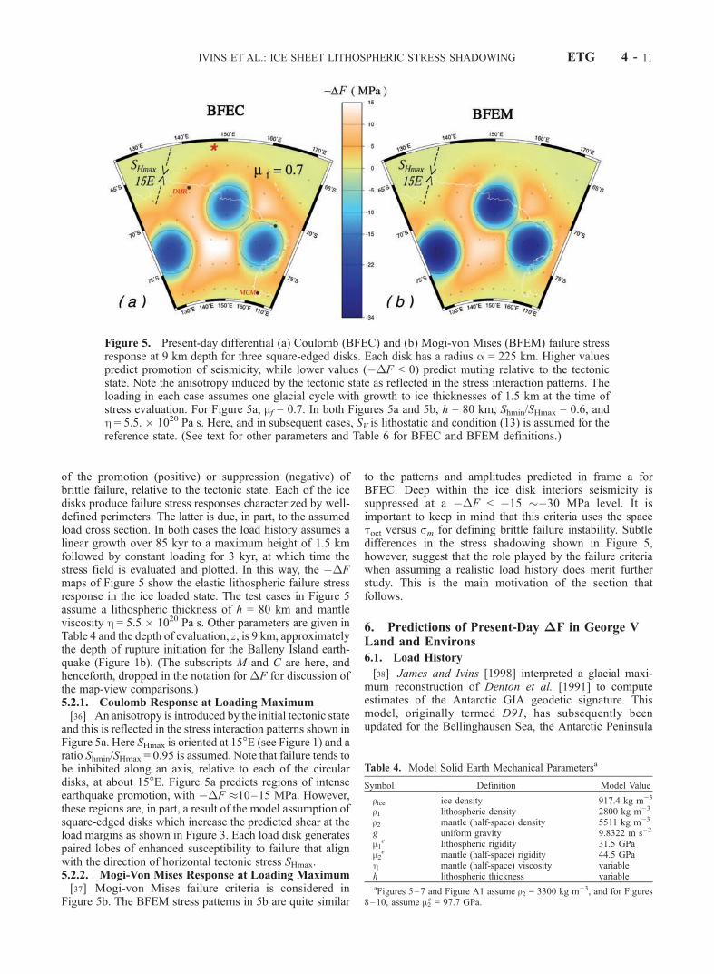
of the promotion (positive) or suppression (negative) ofbrittle failure, relative to the tectonic state. Each of the icedisks produce failure stress responses characterized by well-defined perimeters. The latter is due, in part, to the assumedload cross section. In both cases the load history assumes alinear growth over 85 kyr to a maximum height of 1.5 kmfollowed by constant loading for 3 kyr, at which time thestress field is evaluated and plotted. In this way, the ��Fmaps of Figure 5 show the elastic lithospheric failure stressresponse in the ice loaded state. The test cases in Figure 5assume a lithospheric thickness of h = 80 km and mantleviscosity h = 5.5 � 1020 Pa s. Other parameters are given inTable 4 and the depth of evaluation, z, is 9 km, approximatelythe depth of rupture initiation for the Balleny Island earth-quake (Figure 1b). (The subscripts M and C are here, andhenceforth, dropped in the notation for �F for discussion ofthe map-view comparisons.)5.2.1. Coulomb Response at Loading Maximum[36] An anisotropy is introduced by the initial tectonic state

and this is reflected in the stress interaction patterns shown inFigure 5a. Here SHmax is oriented at 15�E (see Figure 1) and aratio Shmin/SHmax = 0.95 is assumed. Note that failure tends tobe inhibited along an axis, relative to each of the circulardisks, at about 15�E. Figure 5a predicts regions of intenseearthquake promotion, with ��F 10–15 MPa. However,these regions are, in part, a result of the model assumption ofsquare-edged disks which increase the predicted shear at theload margins as shown in Figure 3. Each load disk generatespaired lobes of enhanced susceptibility to failure that alignwith the direction of horizontal tectonic stress SHmax.5.2.2. Mogi-Von Mises Response at Loading Maximum[37] Mogi-von Mises failure criteria is considered in

Figure 5b. The BFEM stress patterns in 5b are quite similar

to the patterns and amplitudes predicted in frame a forBFEC. Deep within the ice disk interiors seismicity issuppressed at a ��F < �15 ��30 MPa level. It isimportant to keep in mind that this criteria uses the spacetoct versus sm for defining brittle failure instability. Subtledifferences in the stress shadowing shown in Figure 5,however, suggest that the role played by the failure criteriawhen assuming a realistic load history does merit furtherstudy. This is the main motivation of the section thatfollows.

6. Predictions of Present-Day �F in George VLand and Environs

6.1. Load History

[38] James and Ivins [1998] interpreted a glacial maxi-mum reconstruction of Denton et al. [1991] to computeestimates of the Antarctic GIA geodetic signature. Thismodel, originally termed D91, has subsequently beenupdated for the Bellinghausen Sea, the Antarctic Peninsula

Table 4. Model Solid Earth Mechanical Parametersa

Symbol Definition Model Value

rice ice density 917.4 kg m�3

r1 lithospheric density 2800 kg m�3

r2 mantle (half-space) density 5511 kg m�3

g uniform gravity 9.8322 m s�2

m1e lithospheric rigidity 31.5 GPa

m2e mantle (half-space) rigidity 44.5 GPa

h mantle (half-space) viscosity variableh lithospheric thickness variableaFigures 5–7 and Figure A1 assume r2 = 3300 kg m�3, and for Figures

8–10, assume m2e = 97.7 GPa.

Figure 5. Present-day differential (a) Coulomb (BFEC) and (b) Mogi-von Mises (BFEM) failure stressresponse at 9 km depth for three square-edged disks. Each disk has a radius a = 225 km. Higher valuespredict promotion of seismicity, while lower values (��F < 0) predict muting relative to the tectonicstate. Note the anisotropy induced by the tectonic state as reflected in the stress interaction patterns. Theloading in each case assumes one glacial cycle with growth to ice thicknesses of 1.5 km at the time ofstress evaluation. For Figure 5a, mf = 0.7. In both Figures 5a and 5b, h = 80 km, Shmin/SHmax = 0.6, andh = 5.5. � 1020 Pa s. Here, and in subsequent cases, SV is lithostatic and condition (13) is assumed for thereference state. (See text for other parameters and Table 6 for BFEC and BFEM definitions.)


and the western Weddell Sea by Ivins et al. [2000, 2002]and tuned to the timing of retreat estimated by Denton andHughes [2000], Goodwin and Zweck [2000], and Hall etal. [2001]. The latest update is termed D91-1.5 [Ivins etal., 2001] and is assumed for the brittle failure analysisreported here. The primary features of D91-1.5 include(1) a reduction of the total mass exchange with the oceanfrom 24.5 (D91) to 12.5 m of eustatic sea level riseequivalent (SLE) and (2) a lengthening of the deglaciationperiod, with initiation at 22 kyr BP and termination at2–0 kyr BP.[39] The modeled deglaciation from 22 to 11 kyr BP is

smaller in the continental interior than in D91. For theRoss Embayment sector and easternmost East Antarctica,2.08 m and 4.17 m SLE remain at 11 kyr BP, respec-tively. Thereafter, the pace of deglaciation increases and by8 kyr the modeled mass loss of these two regions reducesthe remaining SLE to 1.03 m and 2.15 m, respectively. At6 kyr BP the remaining SLE is 1.27 m for the combinedregions. Minor late Holocene change occurs along thecoast, similar to the model of Huybrechts [2002]. Otherfeatures of D91-1.5 glacial loading are discussed inAppendix B.

[40] Since the relevant viscosity range is assumed to beabove 4 � 1020 Pa s, the details of the collapse between5 and 0 kyr BP are found to be relatively unimportant tothe present-day stress predictions. The load historyincludes two prior 100 kyr glacial cycles. No oceanloading is included. The predicted lithospheric stressshadowing, consequently, is that solely caused by Antarc-tic continental glacial isostasy.

6.2. Other Load Considerations

[41] The D91-1.5 model is similar to the ANT5a modelof Nakada et al. [2000] and the A0 model of Huybrechts[2002] in both the timing and magnitude of coastalloading. A brief summary of some important quantitativedifferences among the three models is given in Table 5 forlocations relevant to the present study. The George VLand and Terre Adelie (see Figure 1b) coastal load isadjusted in D91-1.5 to coincide with the mid-Holocene icegrounded near the Mertz-Ninnis and Dumont d’UrvilleTroughs (i.e., near DRV in Figure 1b) [Domack et al., 1991].The load includes a feature quite like the coastal ice dome near113�E, 66.5�S advocated by Goodwin and Zweck [2000].The recent A0 model simulation by Huybrechts [2002] also

Table 5. Ice Load Thicknesses (Meters) Among Recent Deglaciation Models

Dome C Edmondson Pt. Dumont d’Urville Wilkes Basin125�E, 74.95�S (See Maps) DUR (See Maps) at 150�E, 70�S

A0 ANT5aa D91-1.5 A0 ANT5aa D91-1.5 A0 ANT5aa D91-1.5 A0 ANT5aa D91-1.5

16 kyr BP�50 100 294 175 250 732 50 500 666 500 500 1011

7 kyr BP�75 20 89 150 50 244 50 100 222 150 100 337

aLGM heights are taken identical to the 12 kyr values of Nakada et al. [2000]. (See section 6.1 of text for discussion.)

Figure 6. Present-day differential (a) Coulomb (BFEC) and (b) Mogi-von Mises (BFEM) failure stressresponses at 13 km depth computed for the D91-1.5 ice load model with three glacial cycles. Note therobust magnitudes and the similarity of the two predictions for ��F.


features coastal George V Land geometrical complexity inthe loading/unloading history. Since the timing of ANT5aand A0 are similar to D91-1.5 the average thickness ratios(Table 5) may be used to roughly rescale the failure stresspredictions for these alternative ice models.

6.3. Predicted Patterns of Present-Day ��F

[42] The illustrative maps of Figure 5 show the aniso-tropic behavior of the predicted failure patterns and provide

an estimate of the magnitude of GIA stresses that nudge theArchean crust of East Antarctica closer to, or further from,brittle failure. Both the antiquity and tectonics of this region[Goodge and Fanning, 1999; Dalziel and Lawver, 2001] areconsistent with the assumption of an initial stress that isbelow frictional equilibrium.[43] For a depth of 13 km Figure 6 shows the predicted

present-day BFEC and BFEM stresses (Table 6) assumingthe D91-1.5 ice history (section 6.1). The assumedlithospheric thickness (h = 120 km) is identical to thatassumed in both the D91 predictions of Antarctic crustalmotion [James and Ivins, 1998] and in the global modelcomputations for ICE-3G [Tushingham and Peltier,1991]. This value of h and the value for mantle viscosity,h = 8.0 � 1020 Pa s for Figure 6, are within a factor of

Table 6. Initial Stress States for Numerical Parameter Study

State Definition

BFEC below frictional equilibrium - Coulomb criteriaBFEM below frictional equilibrium - Mogi—von Mises criteria

Figure 7. Present-day differential (a) Coulomb (BFEC) and (b)–(c) Mogi-von Mises (BFEM)stresspatterns. All cases assume Earth structure of Table 4 except r2 = 3300 kg/m3. Additionally, h = 1.0 �1021 Pa s, h = 120 km, and Shmin/SHmax = 0.95, and Figure 7a assumes mf = 0.7. Figure 7c assumes atectonic SHmax rotated counterclockwise by 60� from the orientation of N15�E of Figures 7a and 7b.Deglaciation is the same as is assumed in Figure 6 with tectonic stresses and strength parameters asindicated. The red star at the center-top of the map view in Figure 7a is the approximate position of the25 March 1998 (Mw 8.1) Balleny Island earthquake.


0.7–1.3 of the viscosity models that successfully charac-terize GIA processes in northern Europe [Lambeck, 1997;Davis et al., 1999; Milne et al., 2001; Peltier et al.,2002]. The calculations assume a tectonic stress orienta-tion of N35�E, consistent with the great Antarctic plateearthquake (Figure 1b).[44] The predicted pattern of ��F in Figure 6 is

complex, reflecting contributions from load size, timingand disk load pattern. As in the test load case of Figure 5,contours of ��F are somewhat stretched in the direction

of SHmax (N35�E) and show quantitative predictions thatare at a similar level and of similar pattern for the twocriteria. Peak stresses for BFEC seismicity promotion areroughly 1.5 times those of BFEM predictions, whileseismicity diminution is larger by about a factor of 2for BFEM. The juxtaposition of failure enhancement inthe Wilkes Basin with the failure suppression in the RossSea east of the Transantarctic Mountains owes to complexspatiotemporal interactions between adjacent loading andunloading model elements.6.3.1. Tectonic SHmax at N15��E[45] We now consider variations in the orientation of

SHmax since this is so poorly constrained in the region.Stress maps for the same load history and lithosphericthickness are shown in Figure 7 as assumed in Figure 6.Here, however, the assumed SHmax direction is rotatedcounterclockwise 20�. Although in Figures 7a and 7b thestretched contours of ��F rotate approximately 20� coun-terclockwise, the overall effect is small and has littleinfluence on the promoted failure zones. The changes inassumed mantle viscosity (8 � 1020 versus 10 � 1020) anddepth of evaluation (13 versus 9 km) between the compu-tations in Figures 6, 7a, and 7b, respectively, are of minorconsequence to these predictions and comparisons (also seesection 5.1 and Figure 4).6.3.2. Tectonic SHmax at N45��W[46] In situ measurements of principal stresses using

induced fracturing at the Cape Roberts drill site (CRP-3)have recently been reported by Jarrard et al. [2001].While the drill fracture data indicate that a backgroundstress system given by equation (13) is plausible, theorientation of SHmax may be quite different than assumedin the computations for Figures 6a, 6b, 7a, and 7b(N35�E and N15�E, respectively). The N35�E orientationis consistent with the intraplate earthquake rupture solu-tions of Tsuboi et al. [2000], Antolik et al. [2000], andHenry et al. [2000]. In contrast, the CRP-3 data indicate

Figure 8. Present-day differential Mogi-von Mises(BFEM) failure stress response with thick 240 km litho-sphere using the same load history as in Figures 6 and 7.

Figure 9. Present-day Coulomb (BFEC) failure stress pattern for SHmax at (a) 55� and (b) 75�E. Thehalf-space viscosity is h = 8.6 � 1020 Pa s, and the thickness of the lithosphere is h = 150 km,intermediate between Figures 6 and 7 (120 km) and Figure 8 (240 km).


a N45�W direction for SHmax; a 80� counterclockwiserotation with respect to the N35�E orientation assumedfor the computational results in Figure 6. The predictedpatterns of ��F in Figure 7c (with SHmax at N45�W andthe BFEM failure condition) are broadly similar toFigures 7a and 7b. With the N45�W orientation, however,the undulations of the boundaries between promotion andsuppression zones are smaller and this underscores theimportance of the tectonic stress orientation in predictingthe detailed pattern of present-day GIA-induced seismic-ity. Wu et al. [1999] also found a strong sensitivity ofrebound failure stress predictions to the tectonic back-ground field.

6.4. Predictions for Thick Cratonic Lithosphere

[47] In Figure 8 the same initial tectonic stress orientationas assumed in Figure 6 is used with a mantle viscosity of1.0 � 1021, but now with a lithospheric thickness of240 km, double that assumed in Figures 6 and 7. A valueof h = 240 km is an appropriate upper bound for the EastAntarctic craton [Danesi and Morelli, 2000; Fredericksen etal., 2001] since typical modeled thicknesses of thethermal lithosphere exceed those of the correspondingmechanical lithosphere [Pasquale et al., 2001]. For a240 km thick lithosphere, BFEM and BFEC predictionsare similar in pattern and magnitude hence only the BFEMcase is shown in Figure 8. The long wavelength features of

the stress pattern are quite robust at a lithospheric thicknessvalue of h = 240 km.[48] In Figure 9 BFEC predictions of ��F are shown

for h = 150 km with assumed tectonic stress orientationsof N55�E and N75�E. Here a viscosity is assumed that isthe preferred value determined in a recent analysis byMilne et al. [2001] for Fennoscandia (h = 8.6 � 1020 Pa s).The lithospheric thickness (h = 150 km) is within theacceptable range determined by Milne et al. [2001] forFennoscandian rebound models of GPS crustal motiondata. Here long-wavelength features are also promoted,though not as strongly as in the h = 240 km case shown inFigure 8. As in Figure 8, two regions in Figure 9 show thepromotion of Coulomb failure stress to the level of 1 to2 MPa, one within the continental interior in Wilkes Basinand one located several hundred km offshore (shiftingslightly to the east or west depending on the assumedorientation of SHmax). The pattern is akin to surface bulgemigration during postglacial rebound [Wu and Peltier,1982] and the change of sign is seen in other models offailure stress after deglaciation [Klemann and Wolf, 1998;Wu et al., 1999].[49] A thick East Antarctic mechanical lithosphere, of

order 150–240 km, predicts substantial lateral penetrationof failure stress. In fact, it penetrates several hundreds of kmoffshore into the northeastern sector of the Antarctic plateand GIA processes may therefore be partially responsible

Figure 10. Present-day surface vertical motion assuming parameters of Figure 9. The map predictionillustrates the local scale of present-day vertical crustal isostasy associated with the failure stress maps ofthis paper. The positions of the Dumont d’Urville (DUM1) and McMurdo (MCM4) permanent GPStracking stations are also indicated.


for triggering the 25 March 1998 Mw 8.1 Balleny Islandearthquake as suggested by Tsuboi et al. [2000] andKreemer and Holt [2000]. A 120 km thick lithosphereallows for such triggering, but less ubiquitously so, asexemplified in the stress map of Figure 6b.[50] The predicted uplift rate is shown in Figure 10

assuming the Earth structure used for computing brittlefailure stresses in Figure 9. The uplift pattern is alsobroadscale, but is unaffected by the anisotropy associatedwith background tectonic stresses. A similar regionalbroad pattern of uplift is computed assuming a stratifiedmantle and thinner lithosphere with the D91-1.5 loadterminating at 2 kyr BP by Ivins et al. [2001]. The stresspatterns tend to align with the gradients in the upliftpattern and not necessarily with the locus of maximumuplift rate. This is a feature Hicks et al. [2000] recentlynoted in the earthquake patterns of northern coastalNorway.

6.5. Discussion and Future Directions

[51] A shortcoming of the simplified theoretical com-putations of failure stresses presented here is the absenceof layering in the mantle. If a lower mantle wereincluded that has a substantially higher viscosity thanthe upper mantle then larger stresses would be main-tained in the modeled brittle crust. This role of thelower mantle viscosity, with its potential for a oneorder-of-magnitude increase over the value assigned tothe upper mantle, was first discussed by Spada et al.[1991]. It is of note that the Coulomb stresses calculatedby Wu et al. [1999], with a 20� more viscous lowerthan upper mantle, are more robust than those calculatedhere, considering the more youthful unloading involvedfor Antarctica. Klemann and Wolf [1998, 1999] alsodemonstrate that stratification within the crust, litho-sphere and shallow mantle have important influenceson GIA stress relaxation processes in the upper crust.Future models of Antarctic rebound stresses should alsoconsider the role of such stratification. Unlike Fenno-scandia and eastern Canada, however, virtually no datacurrently constrain models of viscous stratification in theAntarctic region.[52] The modeling employed here also makes the sim-

plifying incompressibility assumption, and Wu et al.[1999] have shown that compressibility may enhancethe peak estimates of j�Fj by as much as 30–65%.Although compressibility and viscous stratification areimportant considerations, the uncertain tectonic stressorientation, the poorly constrained load history and theinfluence of strong contrasts in mechanical strength atdepth across the Transantarctic Mountain Ranges[Ritzwoller et al., 2001; Danesi and Morelli, 2001] areadded factors that must weigh upon future strategies forcomputing forward model GIA brittle failure stresses inthe Antarctic plate environment.

Figure A1. Contours of GIA stress components in 2-Dprofile (in MPa) in the top elastic layer (h = 100 km). Anelliptically shaped surface load profile is assumed witht ! 1 and a = 350 km. Also plotted are the failure stresses�FC and �FM with isotropic reference state as in Figure 4with the same failure law parameters. Height at disk centeris 2.25 km, and the densities are as in Figures 3 and 4. Plotsof trr, tqq, and tzz with a = 333 km match those of Johnstonet al. [1998] for the same Earth structure parameters andpeaked parabola.

Figure B1. (opposite) D91-1.5 ice heights in meters for the study region and surrounding areas at (a) 22 kyr, (b) 8 kyr,and (c) 5 kyr BP. Computations of geoid change and crustal uplift rates are presented for the complete D91-1.5 ice model byIvins et al. [2001].


[53] The relative timing and magnitude of deglaciationalso influence GIA driven seismicity. This aspect of thestress predictions will improve as constraints on the glacialhistory tighten in the future. Certain features of the modelspresented, like the contrast in predicted seismicity across theTransantarctic Mountain Ranges between the Ross Embay-ment and Wilkes Basin, are sensitive to the glacial historyand such details need to be tested using improved loadmodels. Ultimately, seismicity observations could providean important way to test models of ongoing rebound in theregion.

7. Summary and Conclusions

[54] Lithospheric thickness has a strong influence on thepredicted patterns of postglacial seismicity. Johnston et al.[1998] also noted the importance of this parameter inmodeling GIA seismicity and faulting in northern Europe.The surface wave tomographic mapping by Danesi andMorelli [2001] and Ritzwoller et al. [2001] reveal a deepseated high-velocity anomaly beneath the crust of EastAntarctica, indicating that a thick elastic lithosphere existsthere. The anomaly extends 200–500 km northwest ofWilkes Land beneath oceanic crust. The crust and upper-most mantle in East Antarctica are associated with one ofthe most ancient of Earth’s cratons [Dalziel, 1991; Borg andDePaolo, 1994]. Thermo-petrologic models for the mechan-ical structure of Archean cratonic continental lithospherefavor a thickness h � 150 km [Rudnick et al., 1998; Jaupartand Mareschal, 1999].

[55] If GIA-induced stresses brought the crust to failure atthe site of the great intraplate earthquake of 25 March1998 (Mw 8.1), some 320 km offshore, the penetrationlength scale must be large. Such a strong lateral penetrationof the GIA failure stresses is promoted by a thicklithosphere. Similarly, Grollimund and Zoback [2000]interpret the stress profile deduced from deep well porepressure changes as reflective of a postglacial flexure,implying that the GIA stresses presently extend some200 km offshore from the former Fennoscandian ice sheetin southwestern Norway. The tectonic stress levels in ournumerical models are large with SHmax � Shmin 25 MPa,which is about equal to the estimated stress drop on themain Balleny Islands subevent of 25 March 1998 [Henryet al., 2000]. Consequently, GIA acts only as a triggeringmechanism if it is, indeed, the cause of this strike slip event.Postglacial loading is a viable mechanism for triggeringstrike slip rupturing outside of the loaded region [Wu andHasegawa, 1996a] especially for favorable preexistingtectonic states [Schultz and Zuber, 1994].[56] We have computed the stress tensor evolution in the

lithosphere with semianalytic techniques for viscoelasticEarth models [Ivins and James, 1999; Thoma and Wolf,1999; Ivins et al., 2000, 2002] and applied differentialCoulomb and Mogi-von Mises fracture criteria to theprediction of seismic failure. Although the numerical valuesof�F differ to within a factor of 1.5–2, the similarity of theCoulomb and Mogi-von Mises stresses (compare panels aand b of Figures 5, 6, and 7) shows that predictions offracture susceptibility are rather insensitive to the assumed

Figure B1. (continued)


failure law. This gives additional credence therefore to GIAstress results which have previously relied solely on Cou-lomb analyses.[57] Our numerical results reveal the importance of

improving the constraints on the regional tectonic stress.While tectonic stress may be reasonably reconstructedfrom the compound rupture interpretation of the BallenyIsland earthquake [Henry et al., 2000; Antolik et al.,2000], the Neogene continental faulting patterns [Wilson,1999] or from the global mantle-lithospheric flow modelsof Steinberger et al. [2001], new crustal borehole stressdata from the western Ross Sea [Jarrard et al., 2001]indicate a quite different orientation for SHmax. It ispossible that the tectonic stress field is spatially heteroge-neous across the vast extent of the northeastern Antarcticplate. Nevertheless, our modeling strongly suggests thatthe Antarctic crust should be seismically active because ofGIA processes, regardless of the details of the tectonicstress state.

Appendix A: Load Shape

[58] As discussed in section 5.1 and 5.2 concern must begiven to the assumed model cross-sectional shape of thecylindrically symmetric load. Calculations with ellipticalcross-section load types is also provided here. Figure A1shows stress contours in 2-D profile in the top elastic layerfor an elliptically shaped surface load profile at t ! 1and a = 350 km. Included are the failure stresses predictedby BFEC (�FC) and BFEM (�FM) assumptions (withlithostatic reference state), the octahedral stress (toct) andthe 4 incremental stress components. These may bedirectly compared to contours plotted for the response tosquare-edged and bell-shaped type disk loading shown inFigures 3 and 4. The total volume of the ice load isidentical to the square-edged case of Figure 3. Note thedifferences between trz and that of a square-edged disk inFigure 3c. Note, again, the promotion of the failurestresses just outside the loaded area. Generally, however,the dimension of the load versus the lithospheric thicknessis also an important consideration. This sensitivity hasbeen the subject of recent studies by Klemann and Wolf[1998] and Johnston et al. [1998]. Although the shapes areimportant when considering shallow fracturing close tothe load margin, the differences between brittle failurepredictions among full deglaciation simulations is small(�10–30%) at depths where seismic energy released inthe crust is greatest (8 < z < 20 km).

Appendix B: Load History

[59] For the purposes of computing the brittle failurestress responses our initial computational simulations in-cluded the full refined disk structures of D91-1.5. However,via iteration, the number of disks was reduced by a factor of3 to enhance computational efficiency. The square edgeddisks that are used for computing Wilkes Land lithosphericresponse in the Antarctic plate are shown in Figure B1 at 22,8, and 5 kyr BP (frames a, b, and c, respectively). Approx-imations are the inclusion of the Ross Sea ice load and aridge of ice disks along the 135�E longitude from about85�S to the Marie Byrd Land Coast. The ridge is a far field

load approximation, having a total mass equivalent to about353 Tt (1 Tt = 1015 kg with 360 Tt corresponding to an icemass sufficient to change global sea level by 1 meter).Within the region of interest (Figure 1b) Last GlacialMaximum (LGM) is simulated using a coarse disk repre-sentation. The Ross sector at LGM has an ice load mass of903 Tt (2.5 m of SLE). Throughout northern VictoriaLand, and for all loads to the west of the TransantarcticMountain Range and east of 90�E (see Figure 1), the LGMload is 1,890 Tt (or 5.25 m SLE).[60] Modeled deglaciation from 22 to 11 kyr BP is of

moderate size in the continental interior, similar to therecent Huybrechts [2002] model. The Ross Embaymentsector and easternmost East Antarctic maintain 2.08 mand 4.17 m SLE respectively, at 11 kyr BP, after whichablation is more rapid. By 8 kyr BP the modeled ice loss ofthe two respective regions reduces the SLE values to 1.03 mand 2.15 m, and by 6 kyr BP the deglaciation model has aremaining SLE 0.14, 0.33 and 0.8 m of mass load equiv-alent for the 135�E ridge, the Ross sector and East Antarc-tica, respectively. The D91-1.5 ice history continuescollapsing and is almost complete by 5 kyr BP. Minor lateHolocene ice change occurs along the coastal disks. Degla-ciation in the model occurs up to AD 1500, and notthereafter. The continent-wide D91-1.5 model has averagenegative mass balance over the last 5 kyr BP that is wellbelow 0.1 mm/yr SLE [Ivins et al., 2001].

[61] Acknowledgments. This work was performed by Jet PropulsionLaboratory, California Institute of Technology, under contract with NASA(ERI), by Pacific Geoscience Centre, an office of the Geological Survey ofCanada (TSJ) and by the SEAL project, German Federal Ministry ofEducation and Research (BMBF) Project SF2000/13 (VK). The authorswish to acknowledge important communications with Bruce Banerdt,Stephan Bannister, Stefania Danesi, Shamita Das, Andrea Donnellan,Masaki Kanao, Paul Lundgren, Carol Raymond, Michael Ritzwoller, SeijiTsuboi and Terry Wilson. Generic Mapping Tools (GMT) software [Wesseland Smith, 1991] produced many of the figures presented in this paper.Constructive reviews by Allison Bent, Ctirad Matyska, Giorgio Spada, andDetlef Wolf are greatly appreciated. Grants from the Solid Earth andNatural Hazards Program of NASA’s Earth Science Office provided thesupport for this research. Geological Survey of Canada Contribution2002195.

ReferencesAdams, J., Postglacial faulting in eastern Canada: Nature, origin and seis-mic hazard implications, Tectonophysics, 163, 323–331, 1989.

Antolik, M., A. Kaverina, and D. S. Dreger, Compound rupture of the great1998 Antarctic plate earthquake, J. Geophys. Res., 105, 23,825–23,838,2000.

Arvidsson, R., Fennoscandian earthquakes: Whole crustal rupturing relatedto postglacial rebound, Science, 274, 744–746, 1996.

Bannister, S., and B. N. L. Kennett, Seismic activity in the TransantarcticMountains—Results from a broadband array deployment, Terra Antarct.,9, 41–46, 2002.

Borg, S. G., and D. J. DePaolo, Laurentia, Australia and Antarctica as aLate Proterozoic supercontinent, Geology, 22, 307–310, 1994.

Brudy, M., M. D. Zoback, K. Fuchs, F. Rummel, and J. Baumgartner,Estimation of the complete stress tensor to 8 km depth in the KTBscientific drill holes: Implications for crustal strength, J. Geophys. Res.,102, 18,453–18,475, 1997.

Candie, S. C., J. M. Stock, R. D. Muller, and T. Ishihara, Cenozoic motionbetween East and West Antarctica, Nature, 404, 145–150, 2000.

Chang, C., and B. Haimson, True triaxial strength and deformability of theGerman Continental Deep Drilling Program (KTB) deep hole amphibo-lite, J. Geophys. Res., 105, 18,999–19,013, 2000.

Dalziel, I. W. D., Pacific margins of Laurentia and East Antarctica –Australia as a conjugate rift pair: Evidence and implications for an Eo-Cambrian supercontinent, Geology, 19, 598–601, 1991.

Dalziel, I. W. D., and L. A. Lawver, The lithospheric setting of the WestAntarctic ice sheet, in The West Antarctic Ice Sheet: Behavior and


Environment, Antarctic Res. Ser., vol. 77, edited by R. B. Alley and R. A.Bindschadler, pp. 29–44, AGU, Washington, D. C., 2001.

Danesi, S., and A. Morelli, Group velocity of Rayleigh waves in theAntarctic region, Phys. Earth Planet. Int., 122, 55–66, 2000.

Danesi, S., and A. Morelli, Structure of the upper mantle under theAntarctic Plate from surface wave tomography, Geophys. Res. Lett., 28,4395–4398, 2001.

Davis, J. L., J. X. Mitrovica, H.-G. Scherneck, and H. Fan, Investigations ofFennoscandian glacial isostatic adjustment using modern sea levelrecords, J. Geophys. Res., 104, 2733–2747, 1999.

Dehls, J. F., O. Olesen, L. Olsen, and L. Harald-Blikra, Neotectonic faultingin northern Norway: The Stuorgurra and Nordmannvikdalen postglacialfaults, Quat. Sci. Rev., 19, 1447–1460, 2000.

Denton, G. H., and T. J. Hughes, Reconstruction of the Ross ice drainagesystem, Antarctica, at the Last Glacial Maximum, Geogr. Ann., Part A,82, 143–166, 2000.

Denton, G. H., M. L. Prentice, and L. H. Burckle, Cainozoic history ofthe Antarctic ice sheet, in Geology of Antarctica, edited by R. J. Tingey,pp. 365–433, Oxford Univ. Press, New York, 1991.

Dietrich, R., et al., ITRF coordinates and plate velocities from repeatedGPS campaigns in Antarctica—An analysis based on different individualsolutions, J. Geod., 74, 756–766, 2001.

Domack, E. W., A. J. T. Jull, and S. Nakao, Advance of East Antarcticoutlet glaciers during the Hypsithermal: Implications for the volume stateof the Antarctic ice sheet under global warming, Geology, 19, 1059–1062, 1991.

Engelder, T., Stress Regimes in the Lithosphere, 459 pp., Princeton Univ.Press, Princeton, N. J., 1992.

Fredericksen, A. W., M. G. Bostock, and J. F. Cassidy, S-wave velocitystructure of the Canadian lithosphere, Phys. Earth Planet. Int., 124, 175–191, 2001.

Gambino, S., and E. Privitera, Characterization of earthquakes recorded byMt. Melborne volcano seismic network (northern Victoria Land, Antarc-tica), Terra Antarct., 1, 167–172, 1994.

Goodge, J. W., and C. M. Fanning, 2.5 b.y. of punctuated Earth history asrecorded in a single rock, Geology, 27, 1007–1010, 1999.

Goodwin, I. D., and C. Zweck, Glacio-isostasy and glacial ice load atLaw Dome, Wilkes Land, East Antarctica, Quat. Res., 53, 285–293,2000.

Grollimund, B., and M. D. Zoback, Post glacial lithospheric flexure andinduced stresses and pore pressure changes in the northern North Sea,Tectonophysics, 327, 61–81, 2000.

Hall, B. L., G. H. Denton, and B. Overturf, Glacial Lake Wright, a high-level Antarctic lake during the LGM and early Holocene, Antarct. Sci.,13, 53–60, 2001.

Hasegawa, H. S., Neotectonics and inferred movements in Canada, Bull.Geol. Surv. Finl., 60, 3–25, 1988.

Henry, C., S. Das, and J. H. Woodhouse, The great March 25, 1998,Antarctic Plate earthquake: Moment tensor and rupture history, J. Geo-phys. Res., 105, 16,097–16,118, 2000.

Hicks, E. C., H. Bungmar, and C. D. Lindholm, Seismic activity, inferredcrustal stresses and seismotectonics in the Rana region, northern Norway,Quat. Sci. Rev., 19, 1423–1436, 2000.

Hill, D. P., Contemporary block tectonics: California and Nevada, J. Geo-phys. Res., 87, 5433–5450, 1982.

Hori, T., and Y. Kaneda, Morgan Hill earthquake in the stress shadow of the1906 San Francisco earthquake, Geophys. Res. Lett., 28, 2261–2264,1911.

Huybrechts, P., Sea-level changes at the LGM from ice-dynamic recon-structions of the Greenland and Antarctic ice sheets during the glacialcycles, Quat. Sci. Rev., 21, 203–231, 2002.

Ivins, E. R., and T. S. James, Simple models for late Holocene and present-day Patagonian glacier fluctuations and predictions of a geodeticallydetectable isostatic response, Geophys. J. Int., 138, 601–625, 1999.

Ivins, E. R., T. H. Dixon, and M. P. Golombek, Extensional reactivationof an abandoned thrust: A bound on shallowing in the brittle regime,J. Struct. Geol., 12, 303–314, 1990.

Ivins, E. R., C. A. Raymond, and T. S. James, The influence of 5000 year-old and younger glacial mass variability on present-day rebound in theAntarctic Peninsula, Earth Planets Space, 52, 1023–1029, 2000.

Ivins, E. R., X. Wu, C. A. Raymond, C. F. Yoder, and T. S. James,Temporal geoid of a rebounding Antarctica and potential measurementby the GRACE and GOCE satellites, in I. A. G. Symposia 123: Gravity,Geoid and Geodynamics 2000, edited by M. G. Sideris, pp. 361–366,Springer-Verlag, New York, 2001.

Ivins, E. R., C. A. Raymond, and T. S. James, Late-Pleistocene, Holoceneand present-day ice load evolution in the Antarctic Peninsula: Modelsand predicted vertical crustal motion, in Ice Sheets, Sea Level andthe Dynamic Earth, Geodyn. Ser., vol. 29, edited by J. X. Mitrovicaand B. L. A. Vermeersen, pp. 133–154, AGU, Washington, D. C., 2002.

Jaeger, J. C., Elasticity, Fracture and Flow With Engineering and Geolo-gical Applications, 268 pp., Chapman and Hall, New York, 1969.

James, T. S., and A. L. Bent, A comparison of eastern North Americanseismic strain-rates to glacial rebound strain-rates, Geophys. Res. Lett.,19, 2127–2130, 1994.

James, T. S., and E. R. Ivins, Predictions of Antarctic crustal motions drivenby present-day ice sheet evolution and by isostatic memory of the LastGlacial Maximum, J. Geophys. Res., 103, 4993–5017, 1998.

Jarrard, R. D., D. Moos, T. J. Wilson, C. J. Bucker, and T. S. Paulsen, Stresspatterns observed by borehole televiewer logging of the CRP-3 drillhole,Victoria Land Basin, Antarctica, Terra Antarct., 8, 203–211, 2001.

Jaupart, C., and J. C. Mareschal, The thermal structure and thickness ofcontinental roots, Lithos, 48, 93–114, 1999.

Johnston, A. C., The effect of large ice sheets on earthquake genesis, inEarthquakes at North American Passive Margins: Neotectonics and Post-glacial Rebound, NATO ASI Ser., Ser. C, vol. 266, edited by S. Gregersenand P. W. Basham, pp. 581–599, Springer-Verlag, New York, 1989.

Johnston, P., P. Wu, and K. Lambeck, Dependence of horizontal stressmagnitude on load dimension in glacial rebound models, Geophys.J. Int., 132, 41–60, 1998.

Jones, S., Late Quaternary faulting and neotectonics, south Victoria Land,Antarctica, J. Geol. Soc. London, 154, 645–652, 1996.

Kanamori, H., and E. E. Brodsky, The physics of earthquakes, Phys. Today,102, 34–40, 2001.

King, G. C. P., R. S. Stein, and J. Lin, Static stress changes and thetriggering of earthquakes, Bull. Seismol. Soc. Am., 84, 935–953, 1994.

Klemann, V., and D. Wolf, Modelling of stresses in the Fennoscandianlithosphere induced by Pleistocene glaciations, Tectonophysics, 294,291–303, 1998.

Klemann, V., and D. Wolf, Implications of a ductile layer for the deforma-tion caused by the Fennoscandian ice sheet, Geophys. J. Int., 139, 216–226, 1999.

Kreemer, C., and W. E. Holt, What caused the March 25, 1998 Antarcticplate earthquake?: Inferences from regional stress and strain rate fields,Geophys. Res. Lett., 27, 2297–2300, 2000.

Kuge, K., M. Kikuchi, and Y. Yamanaka, Non-double-couple momenttensor of the March 25, 1998 Antarctic earthquake: Composite ruptureof strike-slip and normal faults, Geophys. Res. Lett., 26, 3401–3404,1999.

Lagerback, R., Neotectonic structures in northern Sweden, Geol. Foeren.Stockholm Foerh., 100, 263–269, 1979.

Lagerback, R., Dating of late Quaternary faulting in northern Sweden,J. Geol. Soc. London, 149, 285–292, 1992.

Lambeck, K., Sea-level changes along the French Atlantic and channelcoasts since the time of the Last Glacial Maximum, Palaeogeogr.Palaeoclimatol. Palaeoecol., 129, 1–22, 1997.

Malvern, L. E., Introduction to the Mechanics of a Solid Medium, 713 pp.,Prentice-Hall, Old Tappan, N. J., 1969.

Milne, G. A., J. L. Davis, J. X. Mitrovica, H. G. Scherneck, J. M. Johansson,M. Vermeer, and H. Koivula, Space-geodetic constraints on glacialisostatic adjustment in Fennoscandia, Science, 291, 2381–2385, 2001.

Mogi, K., Fracture and flow of rocks under high triaxial compression,J. Geophys. Res., 76, 1255–1269, 1971.

Morein, G., D. L. Turcotte, and A. Gabrielov, On the statistical mechanicsof distributed seismicity, Geophys. J. Int., 131, 552–558, 1997.

Muir-Wood, R., Extraordinary deglaciation reverse faulting in northernFennoscandia, in Earthquakes at North American Passive Margins:Neotectonics and Postglacial Rebound, NATO ASI Ser., Ser. C,vol. 266, edited by S. Gregersen and P. W. Basham, pp. 141–174,Springer-Verlag, New York, 1989.

Nakada, M., R. Kimura, J. Okuno, K. Moriwaki, H. Miura, and H. Mae-moku, Late Pleistocene and Holocene melting history of the Antarctic icesheet derived from relative sea-level variations,Mar. Geol., 167, 85–103,2000.

O’Keefe, K., and P. Wu, Effect of mantle structure on postglacial inducedhorizontal displacement, in Ice Sheets, Sea Level and the Dynamic Earth,Geodyn. Ser., vol. 29, edited by J. X. Mitrovica and B. L. A. Vermeersen,pp. 109–118, AGU, Washington, D. C., 2002.

Pasquale, V., M. Verdoya, and P. Chiozzi, Heat flux and seismicity in theFennocandian Shield, Phys. Earth Planet. Int., 126, 147–162, 2001.

Peltier, W. R., I. Shennan, R. Drummond, and B. Horton, On the postglacialisostatic adjustment of the British Isles and the shallow viscoelasticstructure of the Earth, Geophys. J. Int., 148, 443–475, 2002.

Pondrelli, S., and R. Azzara, Upper mantle anisotropy in Victoria Land(Antarctica), Pure Appl. Geophys., 151, 433–442, 1998.

Reading, A. M., Antarctic seismicity and neotectonics, in Antarctica at theClose of a Millennium, Proc. 8th International Symposium on AntarcticEarth Science, Wellington, N. Z., July, 1999, edited by J. A Gamble,D. N. B. Skinner, and S. Henrys, Bull. R. Soc. N. Z., 35, 479–484,2002.


Ritzwoller, M. H., N. M. Shapiro, A. L. Levshin, and G. M. Leahy, Crustaland upper mantle structure beneath Antarctica and surrounding oceans,J. Geophys. Res., 106, 30,645–30,670, 2001.

Roult, G., J.-P. Montagner, E. Stutzmann, S. Barbier, and G. Guiveneux,The GEOSCOPE program: Its data center, Phys. Earth Planet. Int., 113,25–43, 1999.

Rudnick, R. L., W. F. McDonough, and R. J. O’Connell, Thermal structure,thickness and composition of continental lithosphere, Chem. Geol., 145,395–411, 1998.

Salvini, F., G. Brancolini, M. Busetti, F. Storti, F. Mazzarini, and F. Coren,Cenozoic geodynamics of the Ross Sea region, Antarctica: Crustalextension, intraplate strike-slip faulting, and tectonic inheritance, J. Geo-phys. Res., 102, 24,669–24,696, 1997.

Schultz, R. A., and M. T. Zuber, Observations, models and mechanisms offailure of surface rocks surrounding planetary surface loads, J. Geophys.Res., 99, 14,691–14,702, 1994.

Sneddon, I. H., The Use of Integral Transforms, 539 pp., McGraw-Hill,New York, 1972.

Spada, G., D. A. Yuen, R. Sabadini, and E. Boschi, Lower mantle viscosityconstrained by seismicity around deglaciated regions, Nature, 351, 53–55, 1991.

Stein, R. S., The role of stress transfer in earthquake occurrence, Nature,402, 605–609, 1999.

Steinberger, B., H. Schmeling, and G. Marquart, Large-scale lithosphericstress field and topography induced by global mantle circulation, EarthPlanet. Sci. Lett., 186, 75–91, 2001.

Storti, F., F. Rossetti, and F. Salvini, Structural architecture and displace-ment accommodation mechanisms at the termination of the PriestleyFault, northern Victoria Land, Antarctica, Tectonophysics, 341, 141–161, 2001.

Sugden, D. E., M. A. Summerfield, G. H. Denton, T. I. Wilch, W. C.McIntosh, D. R. Marchant, and R. H. Rutford, Landscape developmentin the Royal Society Range, southern Victoria Land, Antarctica: Stabilitysince the mid-Miocene, Geomorphology, 28, 181–200, 1999.

Summerfield, M. A., F. M. Stuart, H. A. P. Cockburn, D. E. Sugden, G. H.Denton, T. Dunai, and D. R. Marchant, Long-term rates of denudationin the Dry Valleys, Transantarctic Mountains, southern Victoria Land,Antarctica based on in-situ-produced cosmogenic 21Ne, Geomorphology,27, 113–129, 1999.

Thoma, M., and D. Wolf, Bestimmung der Mantelviscositat aus Beobach-tungen der Landhebung und Schwere in Fennoskandien, GFZ PotsdamSci. Tech. Rep. STR99/02, 101 pp., GeoForschungsZentrum, Potsdam,Germany, 1999.

Tsuboi, S., M. Kikuchi, Y. Yamanaka, and M. Kanao, The March 25, 1998Antarctic earthquake: Great earthquake caused by postglacial rebound,Earth Planets Space, 52, 133–136, 1998.

Tushingham, A. M., and W. R. Peltier, ICE-3G: A new global model oflate Pleistocene deglaciation based upon geophysical predictions of post-glacial relative sea-level, J. Geophys. Res., 96, 4497–4523, 1991.

Van der Wateren, F. M., and S. A. P. L. Cloetingh, Feedbacks of thelithosphere dynamics and environmental change of the Cenozoic WestAntarctic rift system, Global Planet. Change, 23, 1–24, 1999.

Wessel, P., and W. H. F. Smith, Free software helps map and display data,Eos Trans. AGU, 72, 65–81, 1991.

Wilson, T. J., Cenozoic transtension along the Transantarctic Mountains-West Antarctic rift boundary, southern Victoria Land, Antarctica,Tectonics, 14, 531–545, 1995.

Wilson, T. J., Cenozoic structural segmentation of the Transantarctic Moun-tains rift flank in southern Victoria Land, Global Planet. Change, 23,105–127, 1999.

Wolf, D., The normal modes of a layered, incompressible Maxwell half-space, J. Geophys., 57, 106–117, 1985.

Wolf, D., Viscoelastodynamics of a stratified, compressible planet, incre-mental field equations and short- and long-time asymptotes, Geophys.J. Int., 104, 401–417, 1991.

Wolf, D., Gravitational viscoelastodynamics, Acta Geod. Geophys. Hung.,37, 29–60, 2002.

Wu, P., and H. S. Hasegawa, Induced stresses and fault potential in easternCanada due to a disc load: A preliminary analysis, Geophys. J. Int., 125,415–430, 1996a.

Wu, P., and H. S. Hasegawa, Induced stresses and fault potential in easternCanada due to a realistic load: A preliminary analysis, Geophys. J. Int.,127, 215–229, 1996b.

Wu, P., and P. Johnston, Can deglaciation trigger earthquakes in N. America?,Geophys. Res. Lett., 27, 1323–1326, 2000.

Wu, P., and W. R. Peltier, Viscous gravitational relaxation, Geophys. J. R.Astron. Soc., 70, 435–485, 1982.

Wu, P., P. Johnston, and K. Lambeck, Postglacial rebound and faultinstability in Fennoscandia, Geophys. J. Int., 139, 657–670, 1999.

Zoback, M. D., and B. Grollimund, Impact of deglaciation on present-dayintraplate seismicity in eastern North America and western Europe, C. R.Acad. Sci., Ser. IIa Sci. Terre Planetes, 333, 23–33, 2001.

Zoback, M. L., and World Stress Map and Lithosphere Program TeamMembers, Global patterns of tectonic stress, Nature, 341, 291–298,1989.

Zwartz, D., M. Bird, J. Stone, and K. Lambeck, Holocene sea-level changeand ice-sheet history in the Vestfold Hills, East Antarctica, Earth Planet.Sci. Lett., 155, 131–145, 1998.

��E. R. Ivins, Jet Propulsion Laboratory, California Institute of Technology,

4800 Oak Grove Drive, MS 300/233, Pasadena, CA 91109, USA.([email protected])T. S. James, Geological Survey of Canada, Sidney, B. C., Canada V8L

4B2.V. Klemann, GFZ Potsdam, Geodesy and Remote Sensing, Telegrafen-

berg, D-14473 Potsdam, Germany.


Glacial isostatic stress shadowing by the Antarctic ice sheet

Documents

Transcript of Glacial isostatic stress shadowing by the Antarctic ice sheet