G.J. Lastman,*N.K. Sinha* Department of Applied ...€¦ · Control system design and analysis...
10
Control system design and analysis package G.J. Lastman,*N.K. Sinha* "Department ofApplied Mathematics, University of Waterloo, Waterloo, Ontario, Canada N2L 3G1 ^Department ofElectrical and Computer Engineering, McMaster University, Hamilton, Ontario, Canada L8S 4L7 Abstract A control system design and analysis package, developed recently by the authors, is described. The entire package fits on a 3.5-inch high density floppy disk, and runs on any IBM compatible personal computer equipped with a numeric co-processor. The package allows the analysis and design ofsingle- input single-output systems using transfer functions or state equations. It is suitable for use by students in an undergraduate engineering program as well as for practising engineers, and runs well under DOS, Windows, and OS/2 Warp. It is very user-friendly and provides information and on-line help in each of the programs. 1 Introduction Teaching control theory, with application to real-life problems usually requires a great deal of computation. Therefore, it is desirable that students have access to reliable computer programs which are easy to use and remove the drudgery out of the numerical computations, so that the students can work out realistic problems that provide the basic understanding of the underlying principles and provide numerical insight. At present several program packages are available commercially, but they tend to be expensive as well as demanding powerful computer hardware. In addition, often they require that a student learn a particularprogramming language, and are not very user-friendly. The present programming package is an attempt to remove these difficulties. This package covers the complete set of computations required in a typical under- graduate course in control systems, while requiring no more space than one high density floppy disk (less than 1.44 megabytes). In addition, on-line help Transactions on Engineering Sciences vol 11, © 1996 WIT Press, www.witpress.com, ISSN 1743-3533
Transcript of G.J. Lastman,*N.K. Sinha* Department of Applied ...€¦ · Control system design and analysis...

Control system design and analysis package
G.J. Lastman,*N.K. Sinha*
"Department of Applied Mathematics, University of Waterloo,
Waterloo, Ontario, Canada N2L 3G1
Department of Electrical and Computer Engineering, McMaster
University, Hamilton, Ontario, Canada L8S 4L7
Abstract
A control system design and analysis package, developed recently by theauthors, is described. The entire package fits on a 3.5-inch high densityfloppy disk, and runs on any IBM compatible personal computer equipped witha numeric co-processor. The package allows the analysis and design of single-input single-output systems using transfer functions or state equations. It issuitable for use by students in an undergraduate engineering program as wellas for practising engineers, and runs well under DOS, Windows, and OS/2Warp. It is very user-friendly and provides information and on-line help ineach of the programs.
1 Introduction
Teaching control theory, with application to real-life problems usually requiresa great deal of computation. Therefore, it is desirable that students haveaccess to reliable computer programs which are easy to use and remove thedrudgery out of the numerical computations, so that the students can work outrealistic problems that provide the basic understanding of the underlyingprinciples and provide numerical insight. At present several program packagesare available commercially, but they tend to be expensive as well as demandingpowerful computer hardware. In addition, often they require that a studentlearn a particular programming language, and are not very user-friendly. Thepresent programming package is an attempt to remove these difficulties. Thispackage covers the complete set of computations required in a typical under-graduate course in control systems, while requiring no more space than onehigh density floppy disk (less than 1.44 megabytes). In addition, on-line help
Transactions on Engineering Sciences vol 11, © 1996 WIT Press, www.witpress.com, ISSN 1743-3533

64 Software for Electrical Engineering
is available, and the user can obtain necessary information about each programdirectly from the package. The hardware requirements are minimal, as theprogram runs quite fast even on a 80386-based computer. However, it isdesirable that the computer be equipped with a numeric co-processor, in viewof the large number of complex numerical computations required for most ofthe programs. In fact, these programs can serve most of the needs of apractising control engineer. Since most of the programs also provide graphicaloutput, a VGA colour monitor is required.
The program package contains a suite of programs which can also beused independently, if desired, but it is preferable to run them through thesystems program which acts as the selector program. It will be described inthe next section.
2 The Systems Program
To start this program in the DOS mode, the user need only type the wordSYSTEMS and press the <Enter> key. In the windows mode one may eitherinstall it as a program item and double click on the corresponding icon, or runit through the file menu. In the OS/2 Warp platform, it will be run as a DOSprogram by clicking on the icon corresponding to the program. The followingmenu appears on the screen, with the cursor highlighting the first program.
Systems
Frequency response of continuous-time linear systemsFrequency response of discrete-time linear systems
Phase plane plot of second-order ordinary differential equationsRoot locus of linear systems
Time-domain response of continuous-time linear systemsNichols Chart method
Design of lead, lag, or lag-lead compensatorsPole-placement compensator design
Solution of the algebraic Riccati equationStability of linear systems by the Routh criterion
Stability of linear systems with parameter uncertaintyState variable feedback for single-input single-output systemsSystem matrices of discrete-time and continuous-time systems
Information about this programExit the systems program
Menu bar: < t >, < 1 > Accept: < Enter >
Figure 1: The main menu
By pressing the down arrow key on the keyboard, the highlight bar maybe moved to the desired item. Pressing the < Enter > key will cause that
Transactions on Engineering Sciences vol 11, © 1996 WIT Press, www.witpress.com, ISSN 1743-3533

Software for Electrical Engineering 65
program to be run. Note that the menu allows the user to obtain informationabout the systems program, and also to exit the program. For example, if thehighlight bar is moved to "Information about this program", and the < Enter >key is pressed, the following is displayed on the screen.
The Systems Program
This program acts as a selector program for a suite of programs forcontinuous-time and discrete-time systems that may arise in control systems.The programs in the suite are
1. Frequency response of continuous-time linear systems (FRPC.Exe)2. Frequency response of discrete-time linear systems (FRPD.Exe)3. Phase plane plot of second-order ordinary differential equations
(Phase. Exe)4. Root locus plot of linear systems (Locus.Exe)5. Time-domain response of continuous-time linear systems
(Response. Exe)6. Nichols Chart method (Nichols.Exe)7. Design of lead, lag, or lag-lead compensators (Compens.Exe)8. Pole-placement compensator design (Pole.Exe)9. Solution of the algebraic Riccati equation (Riccati.Exe)10. Stability of linear systems by the Routh criterion (Routh.Exe)11. Stability of linear systems with parameter uncertainty (Khariton.Exe)12. State variable feedback for single-input, single-output systems
(StateFb.Exe)13. System matrices for discrete-time and continuous-time systems
(SysMat.Exe)
Each program contains on-line information about the program as well as helpexplanations where appropriate. A VGA color monitor is required for allprograms; a color VGA graphics card is required for the graphical output ofprograms 1 to 6. Because of the intensive floating point computations theprograms should be run on a PC with a numeric coprocessor.
Although the 13 programs in this suite of control systems programs havebeen thoroughly tested by the authors, no warranty, express or implied, ismade by the authors as the accuracy and functioning of the programs, norshall the fact of distribution of these programs constitute such warranty, andno responsibility is assumed by the authors in connection therewith.
In particular, these 13 programs should not be relied on for solving aproblem whose incorrect solution could result in injury to a person or loss ofproperty. If you do use the programs in such a way, it is at your own risk.
(C) Copyright 1995 by G.J. Lastman and N.K. Sinha
Figure 2: Screen showing information about the systems program
Transactions on Engineering Sciences vol 11, © 1996 WIT Press, www.witpress.com, ISSN 1743-3533

66 Software for Electrical Engineering
It is seen from figure 2 that the package consists of 13 differentprograms, useful in the analysis and design of control systems, described inreference [1]. These will be described in the following sections.
3 Description of the programs
The first program (FRPC.Exe) displays plots of the frequency responseof a continuous-time linear system from its transfer function, which maycontain an ideal delay. An early version of this program was presented at aconference in 1990 [1]. From the main screen of the program (obtained bypressing the < Enter > key while the corresponding choice is highlighted in themain menu of the systems program), the user can alter the numerator and thedenominator of the transfer function from the default value, alter the desiredfrequency range, alter the value of the delay, and the co-ordinates. Threetypes of plots are available. These are (i) Bode plots, (ii) Gain-phase plot (thegain in decibels is plotted against the phase shift, with the frequency as aparameter along the plot), and (iii) polar plots. All of these plots are usedextensively in the analysis and design of control systems. In each case, theuser can cause a cursor to move along the plot, showing the values of thefrequency, the gain and the phase shift at the location of the cursor. Note thatin the case of Bode plots, both the gain (in decibels) and the phase shift areplotted against the frequency in logarithmic coordinates. To improve thereadability of the plots, the two curves are displayed in different colours,matching the labels on the corresponding coordinate axes. On-line help isavailable from the main menu of this program.
The second program (FRPD.Exe) displays different types of plots of thefrequency response of a discrete-time linear system from its z-transfer function,in a manner similar to the first program.
The third program (Phase.Exe) obtains the plots of the trajectories inthe phase plane of the solution of second-order ordinary differential equations.Although this was originally developed as a graphical method for solvingsecond-order nonlinear differential equations, it is still useful since thetrajectories reveal a great deal of information about the nature of thedifferential equation. In this program we actually use a Runge-Kutta-Fehlberg(RKF45) algorithm to numerically solve the differential equation [3,4] and thenplot it in the phase plane. Thus we combine the power of a good numericalalgorithm with the graphical display of the trajectory. Again, one can use acursor on the graph to reveal the coordinates of any point on the trajectory,including the total time elapsed from the initial point.
The fourth program (Locus.Exe) shows the locus of the roots of theequation
KP + Q = 0where P and Q are polynomials in the complex variable s or z, as theparameter K varies from zero to infinity. In Control Theory this plot is usedto show how the poles of a closed-loop system move in the j-plane (or the z-
Transactions on Engineering Sciences vol 11, © 1996 WIT Press, www.witpress.com, ISSN 1743-3533

Software for Electrical Engineering 67
plane) as the parameter K varies from zero to infinity. An early version of thisprogram was presented in the Electrosoft Conference [5] held in 1993. Here,again, we utilize an efficient algorithm for calculating the roots of the resultingpolynomial for different values of K, and then plot the loci. The user canchoose either the j-plane of the z-plane. For the latter, the unit circle is shownas it is the boundary of stability of the resulting closed-loop systems. As inother programs, a user can move a cursor along the plot, displaying the valuesof the axes, K and the damping ratio at that location of the cursor. Theprogram uses some empirical constants which can be changed by the user.Several problems may arise due to the discrete nature of changes in K as weproceed, and a great deal of effort has gone into ensuring that the plots arecontinuous and accurate. This has required setting up certain empiricalconstants which may have to be changed by the user in some special cases.The information screen for this program provides further details.
The fifth program (Response.Exe) determines and plots the response ofa single-input single-output continuous-time linear system to some "standard"inputs. An earlier version of this program was described in reference [6].The system may be described either in the form of its transfer function or byits state equations. In the latter case, the program uses Leverrier's algorithmto determine the transfer function. The standard inputs considered in theprogram are (i) a unit impulse, (ii) a unit step, (iii) a unit ramp, (iv) cos bt(where the constant b is to be specified by the user), (v) sin bt, (vi) exp(af) cosbt (where the constants a and b are to be specified by the user), and (vii)exp(at) sin bt. Since the ramp function approaches infinity for large f, this isreplaced by the following function
-, for tzar(t) = < a (1)
[ 1, for t>a
The program calculates the transient response of the system to the desired inputby determining the inverse Laplace transform of the product of the transferfunction and the Laplace transform of the input. The analytical expression forthe output is displayed, and the user is given the choice to store it in a file.The program then plots this function against time. Initially the time is takenfrom zero to five times the largest time constant of the system, but the user canspecify the time interval and scale the plot, if desired. If the program findsthat the system is unstable, the user is notified that no plot was attempted sincethe system is unstable.
The sixth program uses a modification of Nichols chart to solve theproblem of designing a compensator so that the maximum value of thefrequency response of the closed-loop system, denoted by M , does not exceeda specified value, usually given in decibels, occurring at a specified frequencyov Originally, control theorists solved this problem by using Nichols chartswhere the main axes are the open-loop gain in decibels and the open-loopphase shift in degrees. Superimposed on this are the curves for constant gain
Transactions on Engineering Sciences vol 11, © 1996 WIT Press, www.witpress.com, ISSN 1743-3533
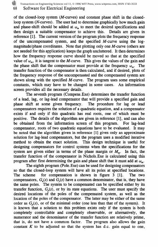
68 Software for Electrical Engineering
of the closed-loop system (Af-curves) and constant phase shift in the closed-loop system (W-curves). The user had to determine graphically how much gainand phase-shift should be added at co to meet the desired specifications andthen design a suitable compensator to achieve this. Details are given inreference [1]. The current version of the program plots the frequency responseof the uncompensated system, and the specified M-curve using the log-magnitude/phase coordinates. Note that plotting only one M-curve (others arenot needed for this application) keeps the graph uncluttered. It then determineshow the frequency response curve should be moved so that at the specifiedvalue of w,%, it is tangent to the M-curve. This gives the values of the gain andthe phase shift that the compensator must provide at the frequency w . Thetransfer function of the compensator is then calculated, and if desired, plots ofthe frequency response of the uncompensated and the compensated system areshown along with the specified M-curve. The program uses some empiricalconstants, which may have to be changed in some cases. An informationscreen provides all the necessary details.
The seventh program (Compens.Exe) determines the transfer functionof a lead, lag, or lag-lead compensator that will provide a specified gain andphase shift at some given frequency. The procedure for lag or leadcompensators requires the solution of a quadratic equation, and a compensatorexists if and only if this quadratic has real roots, one of which must bepositive. The details of the algorithm are given in reference [1], and can alsobe obtained from the information screen of this program. For lag-leadcompensator, roots of two quadratic equations have to be evaluated. It maybe noted that the algorithm given in reference [1] gives only an approximatesolution for lag-lead compensators, but the program uses a modified iterativemethod to obtain the exact solution. This design technique is useful fordesigning compensators for control systems when the specifications for thesystem are given either in terms of the phase margin or M . In fact, thetransfer function of the compensator in Nichols.Exe is calculated using thisprogram after first determining the gain and phase shift that it must add at o .
The eighth program (Pole.Exe) can be used for designing compensatorsso that the closed-loop system will have all its poles at specified locations.The scheme for compensation is shown in figure 3 [1]. The twocompensators, Gj(s) and Gy(s) have a common denominator, that is, they havethe same poles. The system to be compensated can be specified either by itstransfer function, G/J), or by its state equations. The user must specify thedesired locations of the poles of the compensated system, as well as thelocation of the poles of the compensator. The latter may be either of the sameorder as G (s), or of the minimal order (one less than that of the system). Itis known that a solution to this problem exists only if the system is bothcompletely controllable and completely observable, or alternatively, thenumerator and the denominator of the transfer function are relatively prime,that is, do not have a common factor. The program also allows the gainconstant K to be adjusted so that the system has d.c. gain equal to one,
Transactions on Engineering Sciences vol 11, © 1996 WIT Press, www.witpress.com, ISSN 1743-3533

Software for Electrical Engineering 69
corresponding to zero steady-state error to step inputs.
* XO
Figure 3: Pole-placement compensation
The ninth program (Riccati.Exe) can be used for solving the algebraicRiccati equation that occurs in the infinite horizon quadratic regulator problem.The algorithm described in reference [7] is used for this purpose. The solutionis obtained in an iterative manner, as described in the reference, as well as theinformation screen of the program. This program can be useful in introducingan undergraduate class to optimal control theory.
The tenth program (Routh.Exe) uses the Routh criterion of stability todetermine the stability of a continuous-time linear system. This is done byobtaining the Routh table from the denominator polynomial of the transferfunction. Only the first column of the Routh table is displayed, since stabilitydepends only on the number of sign changes in this column. The program alsoallows a user to shift the imaginary axis in the j-plane in order to determinehow close the system is to becoming unstable. The program can also beapplied to determine the stability of discrete-time systems described by theirz-transfer functions. Since the Routh criterion determines the number of rootsof a polynomial with positive real parts, we must introduce a transformationwhich maps the unit circle of the z-plane into the left half of the w-plane. Thisbilinear transformation is given by
w =z-1
(2)
which maps the region inside the unit circle of the z-plane into the left half ofthe >v-plane. The Routh table with the resulting characteristic polynomial isnow calculated and its first column is displayed.
The eleventh program (Khariton.Exe) can be used for determining thestability of linear systems in the more practical situation when there is someuncertainty in the values of one or more parameters. Consider the polynomial
(3)
(4)
-n-l.D(x) = c^"+<
where the upper and lower bounds on the coefficients are given by
Transactions on Engineering Sciences vol 11, © 1996 WIT Press, www.witpress.com, ISSN 1743-3533

70 Software for Electrical Engineering
The independent variable, x, can be either s (for a continuous-time system) orz (for a discrete-time system), and the values of a,, and 6, are given.Normally, to determine the stability of the system, one would have to apply theRouth criterion (after using the bilinear transformation for the discrete-timesystem) to a large number of polynomials formed by all possible differentpolynomials within the intervals of the coefficients.
The recent seminal work of the Russian mathematician Kharitonovmakes it possible to determine stability for systems with coefficients in thespecified ranges through the use of only four "corner" polynomials (seereference [8] for a good description). The Routh criterion is applied to eachof these four polynomials. The system is stable if and only if there is no signchange in the first column of the Routh table for each polynomial.
It may be pointed out that after transformation to the w-plane, andmultiplication by (w-1)*, we get the polynomial
nP(w) = £ c.(w +1)'(w -1)"'' (5)
z=0We note that w= 1 is the image of the point at infinity, which is not a root of
D(z) if apn > 0 The information screen of this program describes how thisdifficulty is overcome, so that the tests on the four polynomials are sufficientbut not necessary for stability with parameter uncertainty.
The twelfth program (StateFb.Exe) can be used to calculate the statefeedback vector that will place the eigenvalues of the closed-loop system atspecified locations. Given the state equations, the program first determines ifthe system is completely controllable. If this condition is satisfied, the matrixfor transforming the system to the controller canonical from is calculated [1].The state feedback vector for this canonical form is easily obtained and thetransformation used to determine the state feedback vector for the original formof the state equations.
The thirteenth program (SysMat.Exe) can be used for determining thestate equations of the corresponding discrete-time system from those of acontinuous-time system, and vice-versa. It is assumed that the continuous-timesystem is sampled at a constant rate and the sampler is followed by a zero-order hold. The sampling interval must be known. The transformation fromthe continuous-time to the discrete-time requires finding the exponential of asquare matrix A, called the system matrix. This can be done by adding aninfinite matrix series, which is uniformly convergent. The series can betruncated after about 15 terms if the sampling interval T is selected so that thespectral radius of AT is less than 0.5. The algorithm is described in most textbooks (for example see [1]). The inverse transformation from discrete-time tocontinuous-time requires finding the natural logarithm of a square matrix. Thisalso is in the form of an infinite series which can be truncated after a certainnumber of terms to obtain desired accuracy. The algorithm used in thisprogram is described in reference [9].
Transactions on Engineering Sciences vol 11, © 1996 WIT Press, www.witpress.com, ISSN 1743-3533

Software for Electrical Engineering 71
4 Conclusions
We have described above the programs in the package developed by us.Each program has on-line help available, and all have built-in exampleproblems for illustration. The programs in this package cover the entirespectrum of computations needed in an undergraduate course on controlsystems. Although we have not included explicitly in this package a programfor determining the transfer function of a single-input single-output systemfrom its state equations, this can be done simply by using the program fortransient response (Response.Exe). Similarly, although we do not have aprogram for designing asymptotic state observers, it is possible to use theprogram StateFb.Exe, due to the duality of the two programs. This isaccomplished by entering the transpose of the -matrix of the system insteadof A, and the vector C instead of B, and then proceeding as in the case of statefeedback. Similarly, one can determine the inverse Laplace transform of arational function through the program Response.Exe. We hope that thesefeatures will make this program package a pleasure to use. As these programsare intended for students, we shall welcome feedback from them.
The programs described in this paper all work well, and have been fullytested by the authors. We shall be glad to share these programs with othersworking in the field and welcome their feedback about the user-friendliness andother suggestions. Participants at the Electrosoft conference are invited tocopy these programs.
At present, there is one short-coming in these programs. The printedcopies of the graphical outputs of the various programs can be obtained onlyby using some commercially available screen-capturing programs (for example,Pizzaz). We would like very much to make the programs independent of thisso that a user can obtain a hard copy without using these commercialprograms. We welcome the suggestions from the participants at theElectrosoft '96 conference, and others on ways to overcome this shortcoming.
References
1. N.K. Sinha, Control Systems, second edition, Wiley Eastern, NewDelhi, 1994.
2. N.K. Sinha, K. Hood and G.J. Lastman, Analysis and design of controlsystems using personal computers, Proceedings of the 33rd MidwestSymposium on Circuits and Systems, Calgary, Alberta, August 1990,pp. 500-503.
3. G.J. Lastman and N.K. Sinha, Microcomputer-based NumericalMethods for Science and Engineering, Holt, Rinehart and Winston,New York, 1989.
Transactions on Engineering Sciences vol 11, © 1996 WIT Press, www.witpress.com, ISSN 1743-3533

72 Software for Electrical Engineering
4. G.E. Forsyth, M.A. Malcolm and C.B. Moler, Computer Methods forMathematical Computations, Prentice-Hall, Englewood Cliffs, NewJersey, 1977.
5. G.J. Lastman and N.K. Sinha, Computer program for root locus plots,Proceedings Electrosoft '93, Southampton, U.K., July 1993, pp. 127-136.
6. N.K. Sinha and G.J. Lastman, System Theory Applications of PersonalComputers - III, LE.E.E. Circuits and Devices Magazine, vol. 5,November 1989, pp. 34-36.
7. P.H. Petkov, N.D. Christov and M.M. Constantinov, ComputationalMethods for Linear Control Systems, Prentice-Hall, Englewood Cliffs,New Jersey, 1991.
8. R.J. Minnichelli, J.J. Anagnost and C.A. Desoer, An elementary proofof Kharitonov's stability theorem, LE.E.E. Transactions on AutomaticControl, vol. AC-34, 1989, pp. 995-998.
9. G.J. Lastman and N.K. Sinha, Infinite series for logarithm of a matrix,applied to identification of linear continuous-time multivariable systemsfrom discrete-time models, Electronics Letters, vol. 27, 1991, pp.1468-1469.
Transactions on Engineering Sciences vol 11, © 1996 WIT Press, www.witpress.com, ISSN 1743-3533