Giving students the run of sprinting models

Andre HeckUniversity of Amsterdam, AMSTEL Institute,

Science Park 904, 1098 XH Amsterdam, The Netherlands∗

Ton EllermeijerUniversity of Amsterdam, AMSTEL Institute†

(Dated: June 2, 2009)

A biomechanical study of sprinting is an interesting and attractive practical investigation taskfor undergraduates and pre-university students who have already done a fair amount of mechanicsand calculus. These students can work with authentic real data about sprinting and carry outpractical investigations similar to the way sports scientists do research. Student research activitiesare viable when the students are familiar with tools to collect and work with data from sensors andvideo recordings, and with modeling tools for comparison of simulation results with experimentalresults. This article presents a multi-purpose system, named coach, which is rather unique in thesense that it offers students and teachers a versatile integrated set of tools for learning, doing, andteaching mathematics and science in a computer-based inquiry approach. Automated tracking ofreference points and correction of perspective distortion in video clips, state-of-the-art algorithmsof data smoothing and numerical differentiation, and graphical system dynamics based modeling,are some of the built-in techniques that are very suitable for motion analysis. Their implementationin coach and their application in student activities involving mathematical models of running arediscussed.

I. INTRODUCTION

The following two types of mathematical models ofrunning are distinguished in the biomechanics literature:

1. kinematic models, based on Newton’s second lawof motion;1–5

2. kinetic models, based on an energy balance for arunner.6–13

All models lead to differential equations for the veloc-ity of the runner. With the exception of a few simplemodels, these differential equations can only be solvednumerically. Computer modeling enables students, whohave already done a fair amount of mechanics and calcu-lus, to relate the theory with results from measurements.Data may come from research literature or from stu-dents’ own measurements. For example, Wagner14 hasdescribed how high school students could use a simplemathematical model to analyze both world record racesof the 100-meter dash and recordings of their own sprintraces.

With the availability of educational video analysis soft-ware such as videopoint

15 and the video tool of log-

ger pro16 to aid experimental investigation, and with

the availability of modeling programs such as stella17

to facilitate the numerical solution of nonlinear differen-tial equations with a minimum of programming effort,the study of the start of a sprint has become a viable,authentic, and attractive investigation for students in aninquiry-based physics course. Strong motives to let stu-dents carry out motion analysis and computer modelingin practical investigations are to bring them into contactwith modern approaches in human movement science andto let them experience that a basic level of mathematics

and physics suffices to do an interesting project similarto the work real motion scientists engage in.

However, one must realize that the research methodsof motion analysis are not simple18–21 and put high de-mands on the quality and ease of use of the tools that aredeployed. One of the most difficult parts of experimen-tal work is getting high-quality data in the first place. Ifpossible, experimental conditions for video recordings areoptimized to ensure the camera can take good videos thatcan be analyzed easily and robustly. For a viable videoanalysis, image processing tools are often indispensableand a robust tracking method must be available to col-lect data in a video recording. Once the data have beencollected, rather advanced data processing tools must beavailable in the tool box, for example to compute use-ful numerical derivatives of measured quantities that aresubject to noise. In the next steps of the investigation itmust be easy to work with the data in conjunction witha nonlinear regression tool and a modeling tool.

Although students can use all kinds of video analysistools and modeling tools in their study of sprinting, itis considered an advantage when these tools have beenintegrated into a single environment so that switchingapplication software and the use of interfacing programsis not needed. In this way, students and teachers onlyneed to familiarize themselves with one environment, inwhich components are geared with each other, and cangrow in their roles of skilled users of the system duringlearning and teaching. A learn-once-use-often philosophyof educational tools is realizable. Such a versatile com-puter environment for learning and doing mathematics,science, and technology in an inquiry approach has beendeveloped in the last twenty-five years at the AMSTELInstitute of the University of Amsterdam. This system,

named coach,22,23 consists of integrated tools for datacollection, for control of processes and devices, for pro-cessing and analyzing data, for modeling, and for au-thoring activities. coach has been translated into sev-eral languages and is used in many countries. In recentyears, this environment has been deployed for variouspractical investigations in movement science by Dutchpre-university students (age 17 to 18).24–27

The rest of this paper is organized as follows. Thecomputer environment coach is briefly described in Sec-tion II, in the light of biomechanical applications. In par-ticular, attention is paid to the correction of perspectivedistortion of planes in video clips, to point tracking asa means for automated video data collection, and to nu-merical differentiation of noisy data, because these meth-ods play an important role in motion analysis. Section IIIreviews various mathematical models of sprinting, illus-trating that only basic levels of mathematics and physicsare needed to understand what is going on. Some resultsof students’ activities are presented in Section IV, illus-trating what even inexperienced users can achieve withcoach. Conclusions about the strength and viability ofthe chosen approach are given in Section V.

II. COACH: A MULTI-PURPOSE

ENVIRONMENT FOR MATHEMATICS AND

SCIENCE EDUCATION

coach has been developed for educational purposes,offering students genuine scientific experiences, but insuch way that it has strong resemblance with contem-porary professional tools. It can be described as a versa-tile learning and authoring environment for mathematics,and science education that integrates tools for

• measurement with interfaces and sensors;

• control of devices (motors, lamps, etc.) and pro-cesses (automated titration, a temperature regula-tor, etc.);

• data video, i.e., measurement on digital video clipsand digital images (capturing of movies included);

• processing and analysis of data (differentiation andintegration, data smoothing, regression analysis,etc.);

• modeling (a text-based, equation-based, and graph-ical approach to system dynamics);

• simulation and animation of modeled phenomena;

• representation of measured data and computed re-sults (graphs, tables, meters, etc.);

• authoring by instructional designers, teachers, andstudents (texts, multimedia components, hyper-links, etc.)

The video analysis, data smoothing and numerical dif-ferentiation facilities, and the graphical modeling tool ofcoach are briefly described, in view of motion analysis.

A. Video analysis

1. Practical issues

In human movement science, analyzing video clips ofhuman body and body part motions is a popular re-search method to study the kinematics and the forcesinvolved.21 The availability of affordable digital videoand computer technology offers students the opportu-nity to actively engage in motion analysis. Educationalprojects that meet this learning goal have already beenreported.24–29 In these projects, students conduct all as-pects of motion analysis: they formulate research ques-tions about a human motion, design experiments, carryout the collection and analysis of video data, and finallyinterpret and report their results. The video analysisequipment used in professional motion laboratories ispowerful, but complicated and expensive, certainly forstudying three-dimensional kinematics. However, for ed-ucational purposes, when mostly planar motions are thesubjects of study, less power and sophistication is needed,and costs can be rather low. A webcam that can recordat a speed of 30 frames per second suffices for data collec-tion in many student projects. In case it is needed, thecost of a good point-and-shoot high-speed camera, e.g.,a CASIO Exilim camera30 that can record at a speed of1000 fps, has dropped to about 300 US$ in 2009. So, evena high-speed camera is now attainable for doing motionanalysis in schools and undergraduate laboratories.

Technology used in motion analysis may changerapidly, but what remains the same in video analysis isthe care needed for the video recording, the data collec-tion, and the data analysis. Educational point-and-clickvideo analysis software such as videopoint

15, and thevideo tool of logger pro

16 and coach22,23 allow stu-

dents to collect position and time data from a recordedvideo clip by using the computer mouse to click in the se-lected frames on the location(s) of the reference point(s)on the moving object(s). However, this manual data col-lection procedure can be time consuming and introduceerrors into the measurements. This holds in particular formotions recorded with a high-speed camera. Automatedtracking of reference points on moving objects is the onlysolution to this problem. This has been implemented incoach.

The experimental setting may also cause problems invideo analysis. For example, it may be impossible inpractice to put the camera fronto-parallel to the planeof motion, leading to a perspective distortion of the im-age. In such a case, image rectification or further dataprocessing is needed to obtain useful position data fromthe video measurements. coach contains a basic set ofnecessary image processing tools.

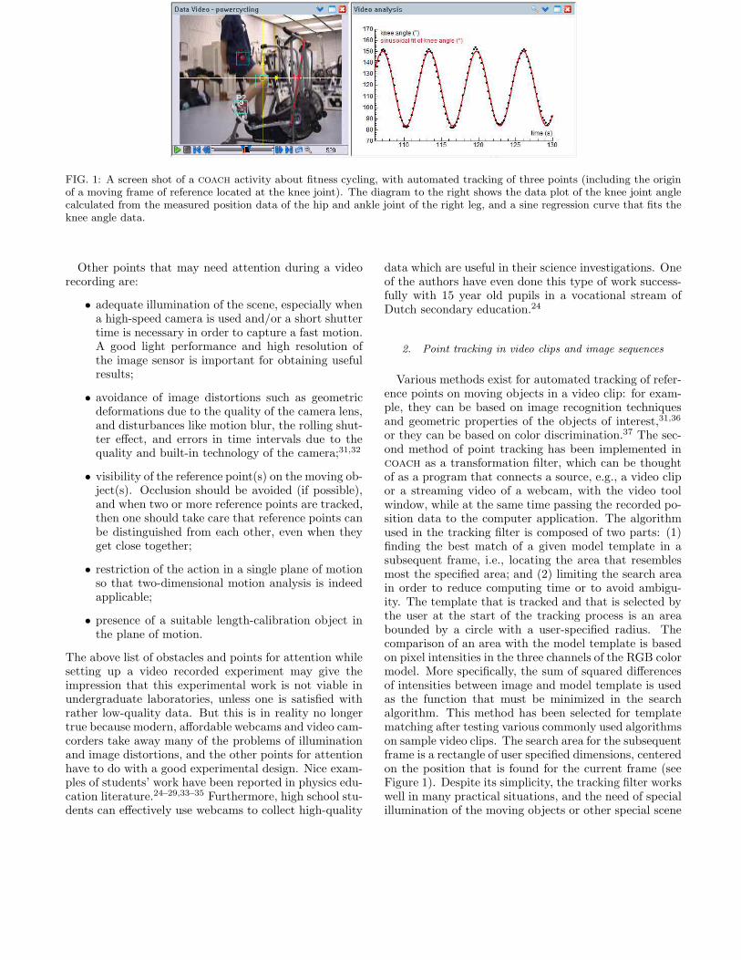
FIG. 1: A screen shot of a coach activity about fitness cycling, with automated tracking of three points (including the originof a moving frame of reference located at the knee joint). The diagram to the right shows the data plot of the knee joint anglecalculated from the measured position data of the hip and ankle joint of the right leg, and a sine regression curve that fits theknee angle data.

Other points that may need attention during a videorecording are:

• adequate illumination of the scene, especially whena high-speed camera is used and/or a short shuttertime is necessary in order to capture a fast motion.A good light performance and high resolution ofthe image sensor is important for obtaining usefulresults;

• avoidance of image distortions such as geometricdeformations due to the quality of the camera lens,and disturbances like motion blur, the rolling shut-ter effect, and errors in time intervals due to thequality and built-in technology of the camera;31,32

• visibility of the reference point(s) on the moving ob-ject(s). Occlusion should be avoided (if possible),and when two or more reference points are tracked,then one should take care that reference points canbe distinguished from each other, even when theyget close together;

• restriction of the action in a single plane of motionso that two-dimensional motion analysis is indeedapplicable;

• presence of a suitable length-calibration object inthe plane of motion.

The above list of obstacles and points for attention whilesetting up a video recorded experiment may give theimpression that this experimental work is not viable inundergraduate laboratories, unless one is satisfied withrather low-quality data. But this is in reality no longertrue because modern, affordable webcams and video cam-corders take away many of the problems of illuminationand image distortions, and the other points for attentionhave to do with a good experimental design. Nice exam-ples of students’ work have been reported in physics edu-cation literature.24–29,33–35 Furthermore, high school stu-dents can effectively use webcams to collect high-quality

data which are useful in their science investigations. Oneof the authors have even done this type of work success-fully with 15 year old pupils in a vocational stream ofDutch secondary education.24

2. Point tracking in video clips and image sequences

Various methods exist for automated tracking of refer-ence points on moving objects in a video clip: for exam-ple, they can be based on image recognition techniquesand geometric properties of the objects of interest,31,36

or they can be based on color discrimination.37 The sec-ond method of point tracking has been implemented incoach as a transformation filter, which can be thoughtof as a program that connects a source, e.g., a video clipor a streaming video of a webcam, with the video toolwindow, while at the same time passing the recorded po-sition data to the computer application. The algorithmused in the tracking filter is composed of two parts: (1)finding the best match of a given model template in asubsequent frame, i.e., locating the area that resemblesmost the specified area; and (2) limiting the search areain order to reduce computing time or to avoid ambigu-ity. The template that is tracked and that is selected bythe user at the start of the tracking process is an areabounded by a circle with a user-specified radius. Thecomparison of an area with the model template is basedon pixel intensities in the three channels of the RGB colormodel. More specifically, the sum of squared differencesof intensities between image and model template is usedas the function that must be minimized in the searchalgorithm. This method has been selected for templatematching after testing various commonly used algorithmson sample video clips. The search area for the subsequentframe is a rectangle of user specified dimensions, centeredon the position that is found for the current frame (seeFigure 1). Despite its simplicity, the tracking filter workswell in many practical situations, and the need of specialillumination of the moving objects or other special scene

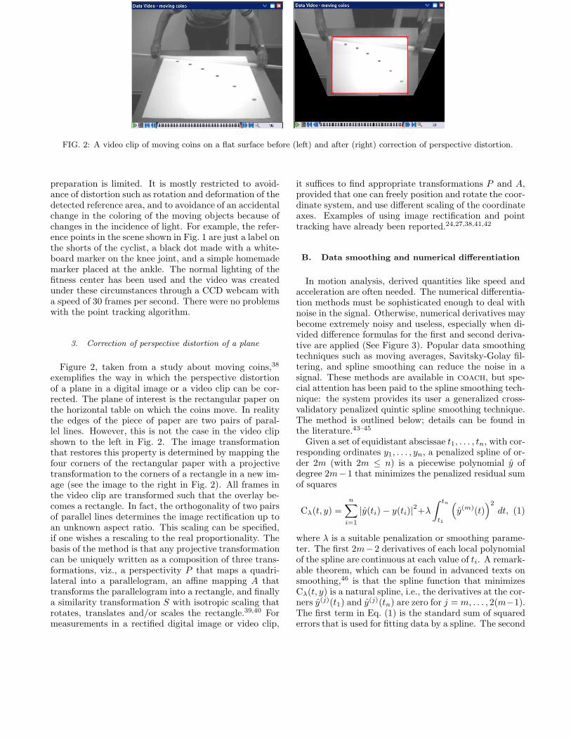
FIG. 2: A video clip of moving coins on a flat surface before (left) and after (right) correction of perspective distortion.

preparation is limited. It is mostly restricted to avoid-ance of distortion such as rotation and deformation of thedetected reference area, and to avoidance of an accidentalchange in the coloring of the moving objects because ofchanges in the incidence of light. For example, the refer-ence points in the scene shown in Fig. 1 are just a label onthe shorts of the cyclist, a black dot made with a white-board marker on the knee joint, and a simple homemademarker placed at the ankle. The normal lighting of thefitness center has been used and the video was createdunder these circumstances through a CCD webcam witha speed of 30 frames per second. There were no problemswith the point tracking algorithm.

3. Correction of perspective distortion of a plane

Figure 2, taken from a study about moving coins,38

exemplifies the way in which the perspective distortionof a plane in a digital image or a video clip can be cor-rected. The plane of interest is the rectangular paper onthe horizontal table on which the coins move. In realitythe edges of the piece of paper are two pairs of paral-lel lines. However, this is not the case in the video clipshown to the left in Fig. 2. The image transformationthat restores this property is determined by mapping thefour corners of the rectangular paper with a projectivetransformation to the corners of a rectangle in a new im-age (see the image to the right in Fig. 2). All frames inthe video clip are transformed such that the overlay be-comes a rectangle. In fact, the orthogonality of two pairsof parallel lines determines the image rectification up toan unknown aspect ratio. This scaling can be specified,if one wishes a rescaling to the real proportionality. Thebasis of the method is that any projective transformationcan be uniquely written as a composition of three trans-formations, viz., a perspectivity P that maps a quadri-lateral into a parallelogram, an affine mapping A thattransforms the parallelogram into a rectangle, and finallya similarity transformation S with isotropic scaling thatrotates, translates and/or scales the rectangle.39,40 Formeasurements in a rectified digital image or video clip,

it suffices to find appropriate transformations P and A,provided that one can freely position and rotate the coor-dinate system, and use different scaling of the coordinateaxes. Examples of using image rectification and pointtracking have already been reported.24,27,38,41,42

B. Data smoothing and numerical differentiation

In motion analysis, derived quantities like speed andacceleration are often needed. The numerical differentia-tion methods must be sophisticated enough to deal withnoise in the signal. Otherwise, numerical derivatives maybecome extremely noisy and useless, especially when di-vided difference formulas for the first and second deriva-tive are applied (See Figure 3). Popular data smoothingtechniques such as moving averages, Savitsky-Golay fil-tering, and spline smoothing can reduce the noise in asignal. These methods are available in coach, but spe-cial attention has been paid to the spline smoothing tech-nique: the system provides its user a generalized cross-validatory penalized quintic spline smoothing technique.The method is outlined below; details can be found inthe literature.43–45

Given a set of equidistant abscissae t1, . . . , tn, with cor-responding ordinates y1, . . . , yn, a penalized spline of or-der 2m (with 2m ≤ n) is a piecewise polynomial y ofdegree 2m−1 that minimizes the penalized residual sumof squares

Cλ(t, y) =

n∑

i=1

|y(ti) − y(ti)|2+λ

∫ tn

t1

(

y(m)(t))2

dt, (1)

where λ is a suitable penalization or smoothing parame-ter. The first 2m−2 derivatives of each local polynomialof the spline are continuous at each value of ti. A remark-able theorem, which can be found in advanced texts onsmoothing,46 is that the spline function that minimizesCλ(t, y) is a natural spline, i.e., the derivatives at the cor-ners y(j)(t1) and y(j)(tn) are zero for j = m, . . . , 2(m−1).The first term in Eq. (1) is the standard sum of squarederrors that is used for fitting data by a spline. The second

term, the integrated square of the mth order derivative,is a measure of the roughness of the data. The parameterλ is the smoothing parameter that controls the trade-offbetween fitting the data by minimizing the residual sumof squares and minimizing the roughness of the approx-imation. With λ = 0, only fitting of the data matters,so an interpolating spline through the data points willbe obtained. As λ increases, more emphasis is placed onpenalizing roughness. As λ → ∞, then only roughnessmatters and the standard least squares fit of the data us-ing a single polynomial of degree m− 1 will be obtained.

There exist data-driven methods for automatic selec-tion of the parameter λ. The generalized cross-validation(GCV) criterion developed by Craven and Wahba47 hasbeen implemented in coach. Although the GCV methodhas been found to be reliable, it is useful to rememberthat it only offers a reasonable smoothing parameter tostart exploratory work. It inevitably involves personaljudgment to select a suitable value of the parameter λ.This is why a user can change or set the value of thesmoothing parameter to see the effect of this action.

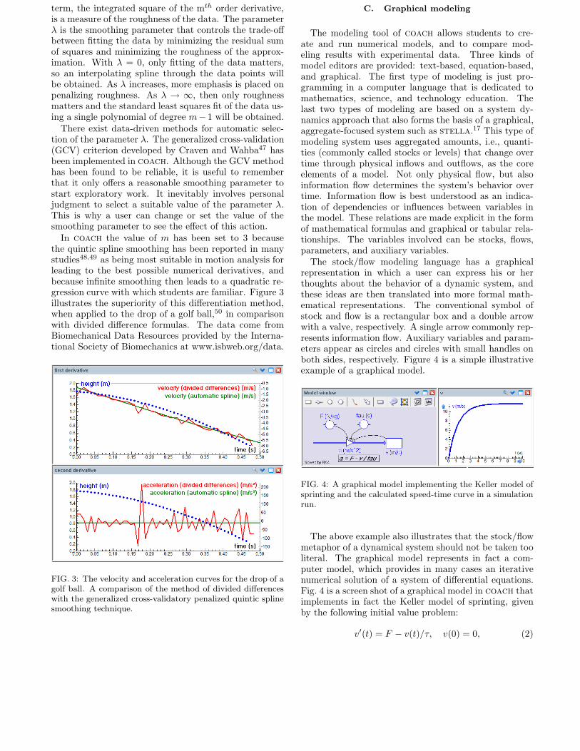
In coach the value of m has been set to 3 becausethe quintic spline smoothing has been reported in manystudies48,49 as being most suitable in motion analysis forleading to the best possible numerical derivatives, andbecause infinite smoothing then leads to a quadratic re-gression curve with which students are familiar. Figure 3illustrates the superiority of this differentiation method,when applied to the drop of a golf ball,50 in comparisonwith divided difference formulas. The data come fromBiomechanical Data Resources provided by the Interna-tional Society of Biomechanics at www.isbweb.org/data.

FIG. 3: The velocity and acceleration curves for the drop of agolf ball. A comparison of the method of divided differenceswith the generalized cross-validatory penalized quintic splinesmoothing technique.

C. Graphical modeling

The modeling tool of coach allows students to cre-ate and run numerical models, and to compare mod-eling results with experimental data. Three kinds ofmodel editors are provided: text-based, equation-based,and graphical. The first type of modeling is just pro-gramming in a computer language that is dedicated tomathematics, science, and technology education. Thelast two types of modeling are based on a system dy-namics approach that also forms the basis of a graphical,aggregate-focused system such as stella.17 This type ofmodeling system uses aggregated amounts, i.e., quanti-ties (commonly called stocks or levels) that change overtime through physical inflows and outflows, as the coreelements of a model. Not only physical flow, but alsoinformation flow determines the system’s behavior overtime. Information flow is best understood as an indica-tion of dependencies or influences between variables inthe model. These relations are made explicit in the formof mathematical formulas and graphical or tabular rela-tionships. The variables involved can be stocks, flows,parameters, and auxiliary variables.

The stock/flow modeling language has a graphicalrepresentation in which a user can express his or herthoughts about the behavior of a dynamic system, andthese ideas are then translated into more formal math-ematical representations. The conventional symbol ofstock and flow is a rectangular box and a double arrowwith a valve, respectively. A single arrow commonly rep-resents information flow. Auxiliary variables and param-eters appear as circles and circles with small handles onboth sides, respectively. Figure 4 is a simple illustrativeexample of a graphical model.

FIG. 4: A graphical model implementing the Keller model ofsprinting and the calculated speed-time curve in a simulationrun.

The above example also illustrates that the stock/flowmetaphor of a dynamical system should not be taken tooliteral. The graphical model represents in fact a com-puter model, which provides in many cases an iterativenumerical solution of a system of differential equations.Fig. 4 is a screen shot of a graphical model in coach thatimplements in fact the Keller model of sprinting, givenby the following initial value problem:

v′(t) = F − v(t)/τ, v(0) = 0, (2)

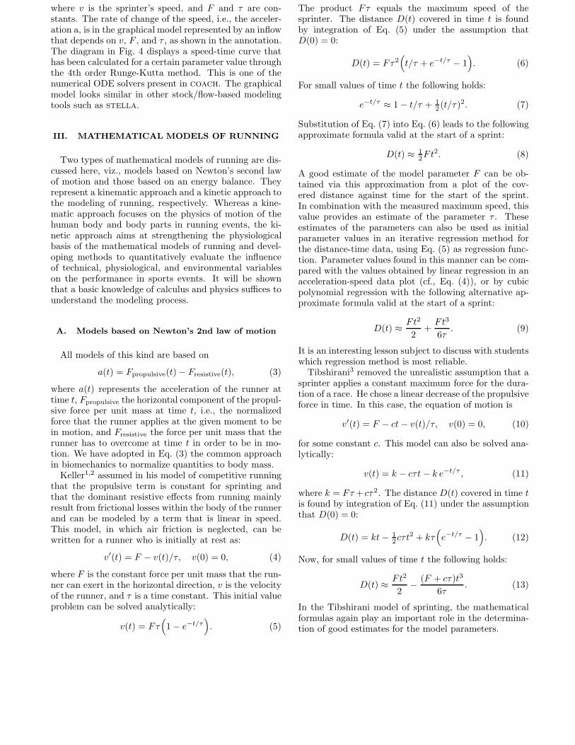
where v is the sprinter’s speed, and F and τ are con-stants. The rate of change of the speed, i.e., the acceler-ation a, is in the graphical model represented by an inflowthat depends on v, F , and τ , as shown in the annotation.The diagram in Fig. 4 displays a speed-time curve thathas been calculated for a certain parameter value throughthe 4th order Runge-Kutta method. This is one of thenumerical ODE solvers present in coach. The graphicalmodel looks similar in other stock/flow-based modelingtools such as stella.

III. MATHEMATICAL MODELS OF RUNNING

Two types of mathematical models of running are dis-cussed here, viz., models based on Newton’s second lawof motion and those based on an energy balance. Theyrepresent a kinematic approach and a kinetic approach tothe modeling of running, respectively. Whereas a kine-matic approach focuses on the physics of motion of thehuman body and body parts in running events, the ki-netic approach aims at strengthening the physiologicalbasis of the mathematical models of running and devel-oping methods to quantitatively evaluate the influenceof technical, physiological, and environmental variableson the performance in sports events. It will be shownthat a basic knowledge of calculus and physics suffices tounderstand the modeling process.

A. Models based on Newton’s 2nd law of motion

All models of this kind are based on

a(t) = Fpropulsive(t) − Fresistive(t), (3)

where a(t) represents the acceleration of the runner attime t, Fpropulsive the horizontal component of the propul-sive force per unit mass at time t, i.e., the normalizedforce that the runner applies at the given moment to bein motion, and Fresistive the force per unit mass that therunner has to overcome at time t in order to be in mo-tion. We have adopted in Eq. (3) the common approachin biomechanics to normalize quantities to body mass.

Keller1,2 assumed in his model of competitive runningthat the propulsive term is constant for sprinting andthat the dominant resistive effects from running mainlyresult from frictional losses within the body of the runnerand can be modeled by a term that is linear in speed.This model, in which air friction is neglected, can bewritten for a runner who is initially at rest as:

v′(t) = F − v(t)/τ, v(0) = 0, (4)

where F is the constant force per unit mass that the run-ner can exert in the horizontal direction, v is the velocityof the runner, and τ is a time constant. This initial valueproblem can be solved analytically:

v(t) = Fτ(

1 − e−t/τ)

. (5)

The product Fτ equals the maximum speed of thesprinter. The distance D(t) covered in time t is foundby integration of Eq. (5) under the assumption thatD(0) = 0:

D(t) = Fτ2(

t/τ + e−t/τ − 1)

. (6)

For small values of time t the following holds:

e−t/τ ≈ 1 − t/τ + 12 (t/τ)2. (7)

Substitution of Eq. (7) into Eq. (6) leads to the followingapproximate formula valid at the start of a sprint:

D(t) ≈ 12Ft2. (8)

A good estimate of the model parameter F can be ob-tained via this approximation from a plot of the cov-ered distance against time for the start of the sprint.In combination with the measured maximum speed, thisvalue provides an estimate of the parameter τ . Theseestimates of the parameters can also be used as initialparameter values in an iterative regression method forthe distance-time data, using Eq. (5) as regression func-tion. Parameter values found in this manner can be com-pared with the values obtained by linear regression in anacceleration-speed data plot (cf., Eq. (4)), or by cubicpolynomial regression with the following alternative ap-proximate formula valid at the start of a sprint:

D(t) ≈Ft2

2+

Ft3

6τ. (9)

It is an interesting lesson subject to discuss with studentswhich regression method is most reliable.

Tibshirani3 removed the unrealistic assumption that asprinter applies a constant maximum force for the dura-tion of a race. He chose a linear decrease of the propulsiveforce in time. In this case, the equation of motion is

v′(t) = F − ct − v(t)/τ, v(0) = 0, (10)

for some constant c. This model can also be solved ana-lytically:

v(t) = k − cτt − k e−t/τ , (11)

where k = Fτ +cτ2. The distance D(t) covered in time tis found by integration of Eq. (11) under the assumptionthat D(0) = 0:

D(t) = kt − 12cτt2 + kτ

(

e−t/τ − 1)

. (12)

Now, for small values of time t the following holds:

D(t) ≈Ft2

2−

(F + cτ)t3

6τ. (13)

In the Tibshirani model of sprinting, the mathematicalformulas again play an important role in the determina-tion of good estimates for the model parameters.

This article describes the use of a graphical modelingtool by students in a sports motion context to createrepresentations of quantities and relationships where an-alytic solutions of equations are too difficult or not pos-sible. The need for computer models is quickly felt whenone wants to take several factors into account for sprint-ing models. For example, the effect of a head- or tailwindcan be translated mathematically into an aerodynamicterm derived completely from air resistance. The empir-ical relation for the drag force is

Fdrag = 12ρ CdA(v − w)2, (14)

where w represents the wind speed (positive and negativevalues indicating tailwind and headwind, respectively), vthe speed of the sprinter, ρ the air density, Cd the dragcoefficient, and A the cross-sectional area of the sprinter.

Other effects on sprint race times like altitude, airpressure, temperature, humidity, curvature of lanes atthe sprint track have been discussed in the researchliterature.51–55 These effects can also be easily incorpo-rated in the computer models.

B. Models based on an energy balance

Many forms of energy besides mechanical energy playa role in the law of conservation of energy when it isapplied to human motion: elastic energy, heat, chemi-cal energy, and so on. In muscles, chemical energy istransformed into mechanical energy. Mechanical energydegrades partly to thermal energy in the case of concen-tric muscle contraction (when the muscle is shortened).It can also be stored in tendons and muscles as elasticenergy, in the case of eccentric muscle contraction (whenthe muscle is extended). A power balance model basedon a supply/demand approach describes the energetics ofmany human motions, including running and other en-durance sports.6 In other words, it means that the sum ofall the rates of flow of energy into and out of the humanbody equals the rate of change of energy of the humanbody. The power balance method, which relates powerproduction and power dissipation, can be written as

Po = Pf +dE

dt+

dH

dt(15)

where Po represents the power which in principle mightbe used to perform movements, Pf the power loss due tofriction, dE/dt the rate of change of external mechanicalenergy (kinetic, rotational and potential energy of thebody), and dH/dt the power loss due to degradation ofmechanical energy into thermal energy. The power pro-duction (Po) is usually the sum of the power productionby the aerobic (Paer) and anaerobic (Pan) energy produc-tion systems:

Po = Paer + Pan. (16)

We discuss below two power balance models of running.

Ward-Smith8 modeled the aerobic and anaerobicpower as follows:

Paer = R(

1 − e−λt)

and Pan = Pmax e−λt, (17)

with R the maximum aerobic power, Pmax the maximumanaerobic power at t = 0, and λ a constant. The expo-nential model of the aerobic power is based on experimen-tal work of Margaria56 and others about oxygen kineticsin a high intensity exercise. Through the anaerobic termit is expressed that the maximal anaerobic power can-not be sustained and decays exponentially. Ward-Smithjustified the mathematical expressions by theoretical ar-guments. In addition, he modeled the thermal power as

dH

dt= α v(t). (18)

The friction term and the rate of change of external me-chanical energy are given in this model by

Pf = Fdrag v = 12ρ CdAv(v − w)2, (19a)

dE

dt=

d(

12mv2

)

dt= mv

dv

dt. (19b)

Substitution of Eqs. (16) to (19b) into Eq. (15) and theassumption that the constants R, Pmax,A, and α are pro-portional to the mass (the tilde ∼ denotes that a quantityis normalized to the body mass m) give

R(

1 − e−λt)

+ Pmaxe−λt =

αv + 12ρ CdA v(v − w)2 + v v′, v(0) = 0.

(20)

This initial value problem can be rewritten as

v′ =1

v

(

R(

1 − e−λt)

+ Pmaxe−λt

−αv − Kv(v − w)2)

, v(0) = 0,(21)

where K = 12ρ CdA. There is only one problem with this

system dynamics equation: the initial velocity v(0) = 0gives an infinite acceleration. Rewriting it as an initialvalue problem of kinetic energy helps:

d(

12v2

)

dt= R

(

1 − e−λt)

+ Pmaxe−λt − α v

−Kv(v − w)2, v(0) = 0.

(22)

Note that the aerobic and anaerobic energy produc-tions are causally related in the Ward-Smith model bythe use of the same time constant λ. More recently,Ward-Smith has introduced separate time constants forthe aerobic and anaerobic energy releases, and he haseven described the anaerobic metabolism with threecomponents.10,11 Following the approach of Peronnet andThibault,12 he has also replaced the assumption that themaximum aerobic power Pmax is constant, by an expo-nential decay after some time interval, in order to be ableto model well middle-distance and long-distance running.

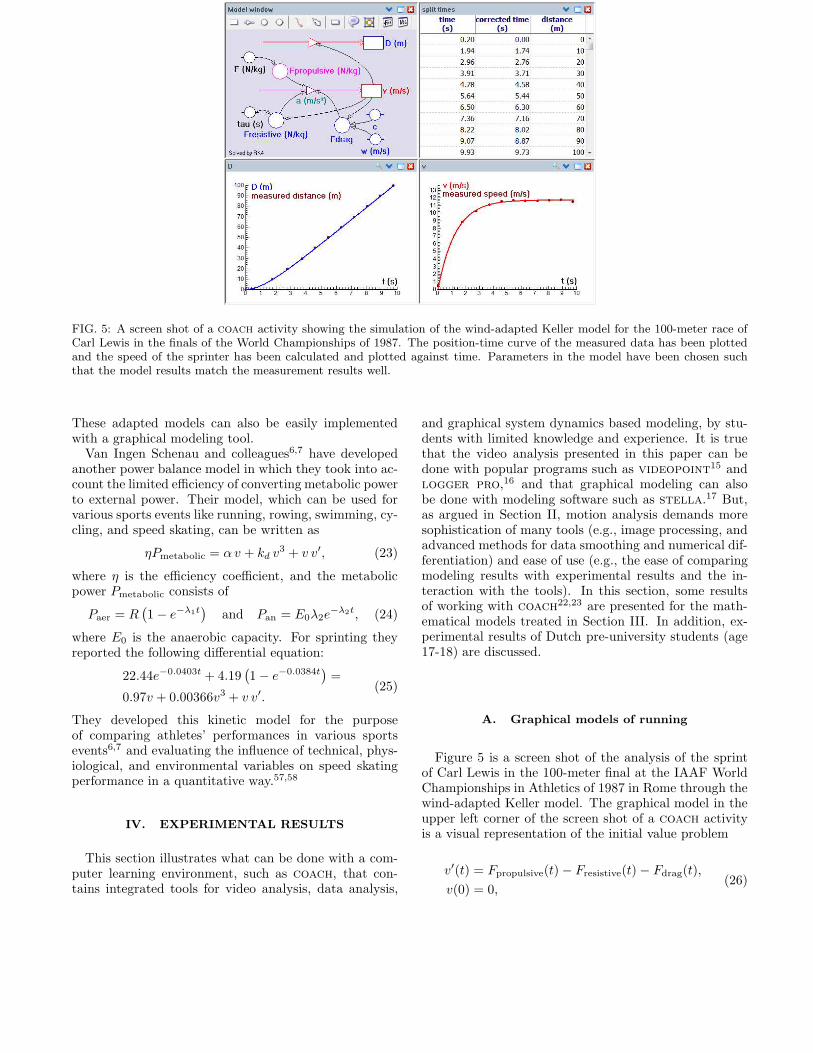
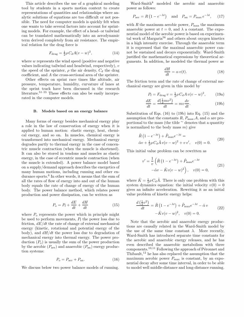
FIG. 5: A screen shot of a coach activity showing the simulation of the wind-adapted Keller model for the 100-meter race ofCarl Lewis in the finals of the World Championships of 1987. The position-time curve of the measured data has been plottedand the speed of the sprinter has been calculated and plotted against time. Parameters in the model have been chosen suchthat the model results match the measurement results well.

These adapted models can also be easily implementedwith a graphical modeling tool.

Van Ingen Schenau and colleagues6,7 have developedanother power balance model in which they took into ac-count the limited efficiency of converting metabolic powerto external power. Their model, which can be used forvarious sports events like running, rowing, swimming, cy-cling, and speed skating, can be written as

ηPmetabolic = α v + kd v3 + v v′, (23)

where η is the efficiency coefficient, and the metabolicpower Pmetabolic consists of

Paer = R(

1 − e−λ1t)

and Pan = E0λ2e−λ2t, (24)

where E0 is the anaerobic capacity. For sprinting theyreported the following differential equation:

22.44e−0.0403t + 4.19(

1 − e−0.0384t)

=

0.97v + 0.00366v3 + v v′.(25)

They developed this kinetic model for the purposeof comparing athletes’ performances in various sportsevents6,7 and evaluating the influence of technical, phys-iological, and environmental variables on speed skatingperformance in a quantitative way.57,58

IV. EXPERIMENTAL RESULTS

This section illustrates what can be done with a com-puter learning environment, such as coach, that con-tains integrated tools for video analysis, data analysis,

and graphical system dynamics based modeling, by stu-dents with limited knowledge and experience. It is truethat the video analysis presented in this paper can bedone with popular programs such as videopoint

15 andlogger pro,16 and that graphical modeling can alsobe done with modeling software such as stella.17 But,as argued in Section II, motion analysis demands moresophistication of many tools (e.g., image processing, andadvanced methods for data smoothing and numerical dif-ferentiation) and ease of use (e.g., the ease of comparingmodeling results with experimental results and the in-teraction with the tools). In this section, some resultsof working with coach

22,23 are presented for the math-ematical models treated in Section III. In addition, ex-perimental results of Dutch pre-university students (age17-18) are discussed.

A. Graphical models of running

Figure 5 is a screen shot of the analysis of the sprintof Carl Lewis in the 100-meter final at the IAAF WorldChampionships in Athletics of 1987 in Rome through thewind-adapted Keller model. The graphical model in theupper left corner of the screen shot of a coach activityis a visual representation of the initial value problem

v′(t) = Fpropulsive(t) − Fresistive(t) − Fdrag(t),

v(0) = 0,(26)

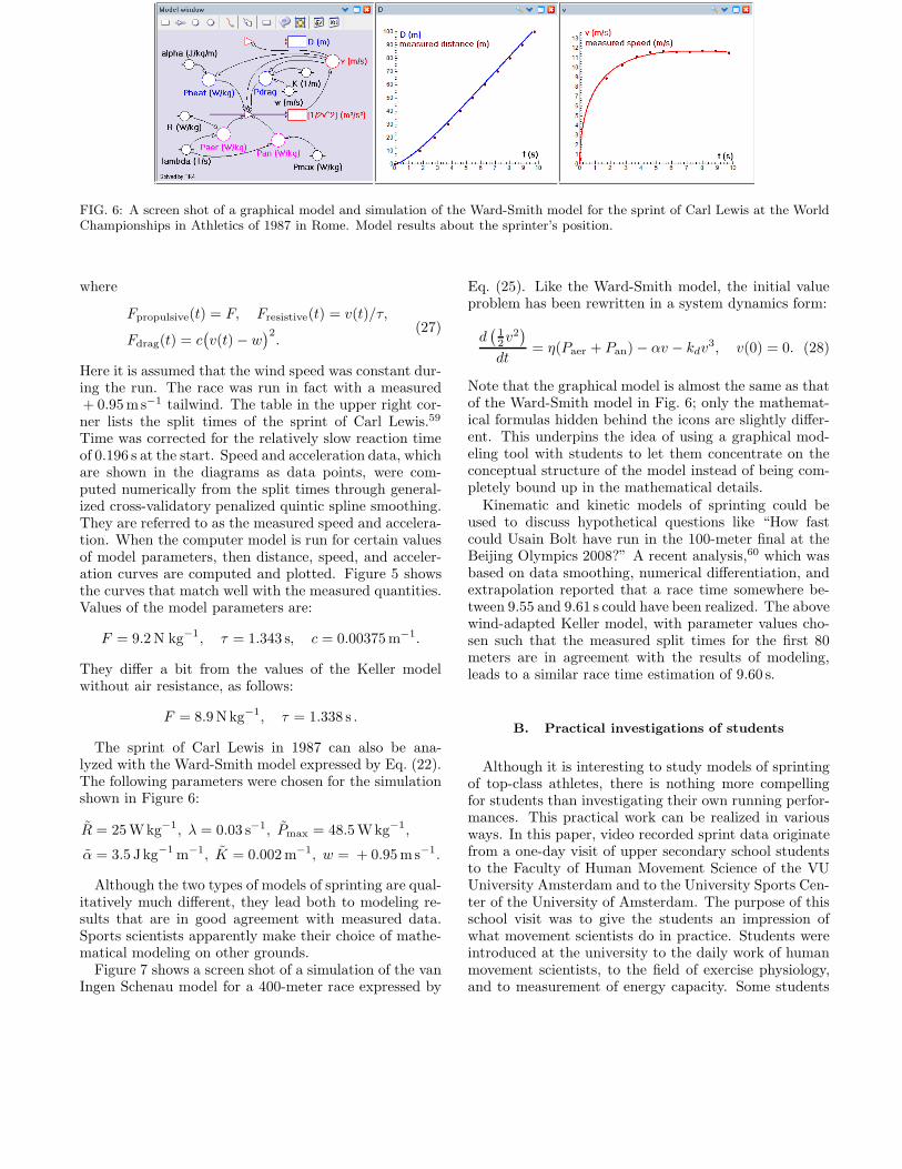
FIG. 6: A screen shot of a graphical model and simulation of the Ward-Smith model for the sprint of Carl Lewis at the WorldChampionships in Athletics of 1987 in Rome. Model results about the sprinter’s position.

where

Fpropulsive(t) = F, Fresistive(t) = v(t)/τ,

Fdrag(t) = c(

v(t) − w)2

.(27)

Here it is assumed that the wind speed was constant dur-ing the run. The race was run in fact with a measured+ 0.95 ms−1 tailwind. The table in the upper right cor-ner lists the split times of the sprint of Carl Lewis.59

Time was corrected for the relatively slow reaction timeof 0.196 s at the start. Speed and acceleration data, whichare shown in the diagrams as data points, were com-puted numerically from the split times through general-ized cross-validatory penalized quintic spline smoothing.They are referred to as the measured speed and accelera-tion. When the computer model is run for certain valuesof model parameters, then distance, speed, and acceler-ation curves are computed and plotted. Figure 5 showsthe curves that match well with the measured quantities.Values of the model parameters are:

F = 9.2 N kg−1, τ = 1.343 s, c = 0.00375 m−1.

They differ a bit from the values of the Keller modelwithout air resistance, as follows:

F = 8.9 Nkg−1, τ = 1.338 s .

The sprint of Carl Lewis in 1987 can also be ana-lyzed with the Ward-Smith model expressed by Eq. (22).The following parameters were chosen for the simulationshown in Figure 6:

R = 25 Wkg−1, λ = 0.03 s−1, Pmax = 48.5 Wkg−1,

α = 3.5 Jkg−1 m−1, K = 0.002 m−1, w = + 0.95 ms−1.

Although the two types of models of sprinting are qual-itatively much different, they lead both to modeling re-sults that are in good agreement with measured data.Sports scientists apparently make their choice of mathe-matical modeling on other grounds.

Figure 7 shows a screen shot of a simulation of the vanIngen Schenau model for a 400-meter race expressed by

Eq. (25). Like the Ward-Smith model, the initial valueproblem has been rewritten in a system dynamics form:

d(

12v2

)

dt= η(Paer + Pan) − αv − kdv

3, v(0) = 0. (28)

Note that the graphical model is almost the same as thatof the Ward-Smith model in Fig. 6; only the mathemat-ical formulas hidden behind the icons are slightly differ-ent. This underpins the idea of using a graphical mod-eling tool with students to let them concentrate on theconceptual structure of the model instead of being com-pletely bound up in the mathematical details.

Kinematic and kinetic models of sprinting could beused to discuss hypothetical questions like “How fastcould Usain Bolt have run in the 100-meter final at theBeijing Olympics 2008?” A recent analysis,60 which wasbased on data smoothing, numerical differentiation, andextrapolation reported that a race time somewhere be-tween 9.55 and 9.61 s could have been realized. The abovewind-adapted Keller model, with parameter values cho-sen such that the measured split times for the first 80meters are in agreement with the results of modeling,leads to a similar race time estimation of 9.60 s.

B. Practical investigations of students

Although it is interesting to study models of sprintingof top-class athletes, there is nothing more compellingfor students than investigating their own running perfor-mances. This practical work can be realized in variousways. In this paper, video recorded sprint data originatefrom a one-day visit of upper secondary school studentsto the Faculty of Human Movement Science of the VUUniversity Amsterdam and to the University Sports Cen-ter of the University of Amsterdam. The purpose of thisschool visit was to give the students an impression ofwhat movement scientists do in practice. Students wereintroduced at the university to the daily work of humanmovement scientists, to the field of exercise physiology,and to measurement of energy capacity. Some students

FIG. 7: A screen shot of a graphical model and simulation of the van Ingen Schenau model for a 400-meter race, showingposition and speed curves.

had the opportunity to measure their oxygen consump-tion in a bicycle ergometer test in the laboratory. Atthe sports center the focus was on research methods tocollect motion data. The students measured their heartrates during running at various intensity levels, and theyassessed their anaerobic capacity via the Wingate cycleergometer test, in which they pedaled at maximal speedfor 30 s against a high braking force. The students alsoused a high-speed camera to record a soccer kick and thetake-off phase of a sprint. In addition, they used a web-cam to record 25-meter sprints of other students in thesports hall. Back at school they analyzed their sprintdata and compared the measured and derived physicalquantities with simulation results from some of the math-ematical models discussed in Section III.

This was actually a viable approach because the stu-dents participating in this project already had experiencewith modeling in coach. They could build the Kellermodel and the Tibshirani model from verbal descriptionsof the model and include aerodynamic effects. The stu-dents were not expected to come up with a kinetic modelthemselves or build a computer model from a verbal de-scription of such kind of mathematical model. We en-visioned the Ward-Smith model as a first example of akinetic model of running to discuss with the students.Based on the implementation of this model in the graph-ical modeling tool, the students would continue withthe study and implementation of the van Ingen Schenaumodel and compare modeling results with their empiricaldata. The power balance models discussed in Section IIIcould provide estimates of the aerobic and anaerobic ca-pacity of the sprinting student. In the project however,the students finally did not apply kinetic models to theirown sprint data. The main reason was that the studentsshould have run a longer distance to really see the differ-ence between kinetic and kinematic models when resultsof modeling are compared with experimental results.

Figure 8 shows the video analysis of a 25-meter sprintof a 16 years old female student running near the wallof the sports hall. Due to the experimental setting, theperspective distortion of the plane of motion could not beavoided in the video recording. But image rectification

through the method outlined in Section II is possible, byusing the wall as rectangular object in the plane of mo-tion. The result is shown in the upper right corner of thescreen shot. Note that the video clip has also been flippedhorizontally to change the direction of motion from leftto right so that the horizontal position and the distanceare the same mathematical notions in a traditional coor-dinate system with the positive axis on the right.

Because the sprint takes about 5 s and the frame rateof the recorded video clip is 30 fps, manual data collec-tion is too time-consuming, error prone, and tedious todo. Therefore, data collection has been done through au-tomated tracking of the sprinter in the video clip. Theresult in the lower left corner of Fig. 8 shows that thismethod is on the one hand applicable even under non-optimal conditions, but on the other hand it may alsolead to rather noisy data. In this particular case, the pe-nalized spline smoothing method outlined in Section IIhelps to obtain a suitable speed-time curve (actually, bymanual selection of an appropriate penalization). Thespeed-time data plot in the lower right corner of Fig. 8 hasbeen approximated by an exponential regression curveaccording to the Keller model of sprinting with a nonzeroinitial velocity (cf., Eq. (5) in Section III):

v(t) = 6.38(

1 − e−0.802t)

+ 1.25 . (29)

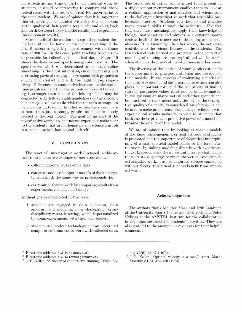
Thus, the time constant τ is about 1.2 s, the initial speed1.25 ms−1, and the maximum speed 7.6 ms−1. Thesevalues correspond with a horizontal propulsive force Fper unit mass of 6.1 Nkg−1 in the Keller model of sprint-ing. These values can be used for the parameters in acomputer model. A simulation of the Keller model withmeasured data points in the background is shown in Fig-ure 9. The descriptive power of the Keller model seemsto be good for the measured sprint data. But when itis used to compute the expected result of a 100-metersprint of this student, the race time of 14 s seems a bitunrealistic for a non-athlete, who is not expected to beable to maintain the maximum speed reached after 20 mfor another 80 m. In other words, the predictive powerof the Keller model is apparently not strong for this run-ning event. The Tibshirani model predicts a seemingly

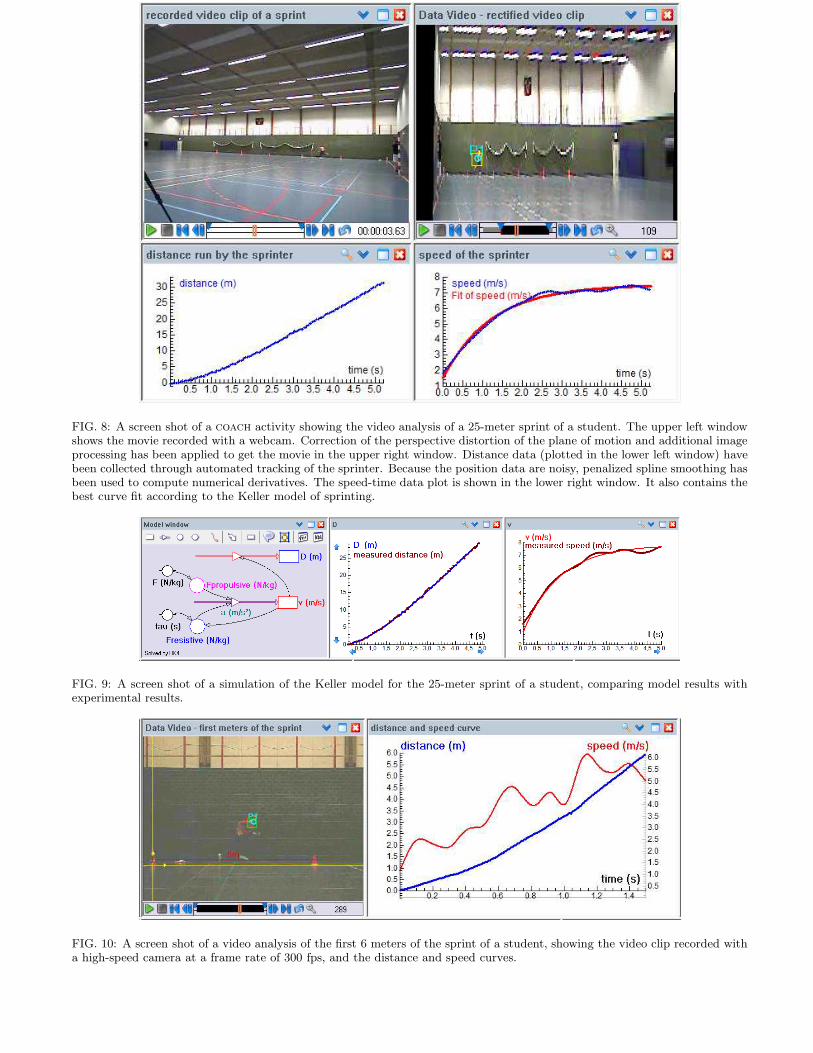
FIG. 8: A screen shot of a coach activity showing the video analysis of a 25-meter sprint of a student. The upper left windowshows the movie recorded with a webcam. Correction of the perspective distortion of the plane of motion and additional imageprocessing has been applied to get the movie in the upper right window. Distance data (plotted in the lower left window) havebeen collected through automated tracking of the sprinter. Because the position data are noisy, penalized spline smoothing hasbeen used to compute numerical derivatives. The speed-time data plot is shown in the lower right window. It also contains thebest curve fit according to the Keller model of sprinting.

FIG. 9: A screen shot of a simulation of the Keller model for the 25-meter sprint of a student, comparing model results withexperimental results.

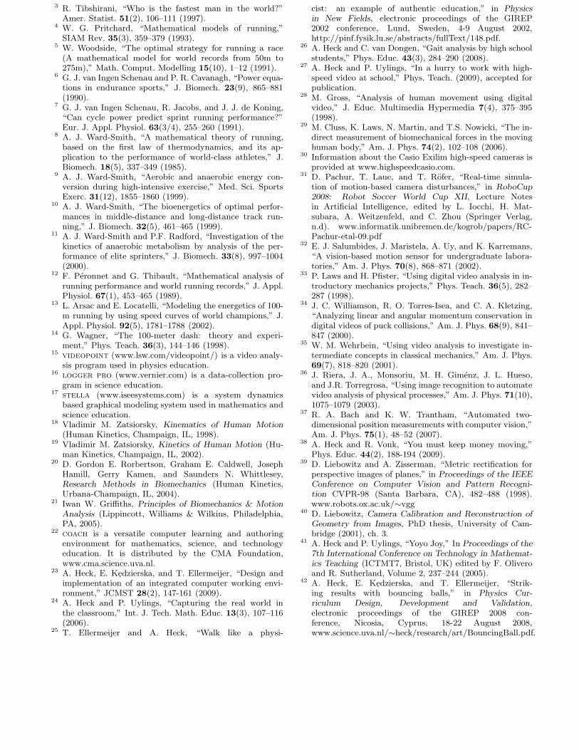
FIG. 10: A screen shot of a video analysis of the first 6 meters of the sprint of a student, showing the video clip recorded witha high-speed camera at a frame rate of 300 fps, and the distance and speed curves.

more realistic race time of 15.4 s. In practical work bystudents, it would be interesting to compare this theo-retical result with the result of a real 100-meter sprint ofthe same student. We are of opinion that it is importantthat students get acquainted with this way of lookingat the quality of their (computer) model and going backand forth between theory (model results) and experiment(measurement results).

More details of the motion of a sprinting student dur-ing take-off can be found in the video recording of thefirst 6 meters using a high-speed camera with a framerate of 300 fps. In this case, point tracking becomes in-dispensable for collecting kinematical data. Figure 10shows the distance and speed-time graphs obtained. Thespeed curve, which was determined by penalized splinesmoothing, is the most interesting curve: increasing anddecreasing parts of the graph correspond with propulsionduring foot contact and with the flight phase, respec-tively. Differences in consecutive increases in the speed-time graph indicate that the propulsive force of the rightleg is stronger than that of the left leg. This may beconnected with left- or right-handedness of the student,but it may also have to do with the runner’s attempts tobalance during take-off. In other words, the speed curveis more than just a bumpy graph: its shape is closelyrelated to the real motion. The goal of this part of theinvestigative work is to let students experience make clearto the students that in mathematics and science a graphis a means, rather than an end in itself.

V. CONCLUSION

The practical, investigative work discussed in this ar-ticle is an illustrative example of how students can

• collect high-quality, real-time data;

• construct and use computer models of dynamic sys-tems in much the same way as professionals do;

• carry out authentic work by comparing results fromexperiments, models, and theory.

Authenticity is interpreted in two ways:

1. students are engaged in data collection, dataanalysis, and modeling in a challenging, cross-disciplinary research setting, which is personalizedby doing experiments with their own bodies;

2. students use modern technology and an integratedcomputer environment to work with collected data.

The broad set of rather sophisticated tools present ina single computer environment enables them to look ata realistic application of mathematics and science andto do challenging investigative work that resembles pro-fessional practice. Students can develop and practicemany research skills through the activities. The factthat they must meaningfully apply their knowledge ofbiology, mathematics, and physics in a concrete sportscontext leads at the same time to deepening and consol-idation of this knowledge. In other words, the activitiescontribute to the science literacy of the students. Theresearch methods learned and practiced in the context ofmodeling of running are prototypical and will be usefulwhen students do practical investigations in other areas.

The diversity of the models of running offers studentsthe opportunity to practice evaluation and revision oftheir models. In the process of evaluating a model onthe basis of experimental data, parameter estimation alsoplays an important role, and the complexity of findingsuitable parameter values must not be underestimated.Initial guessing on mathematical and other grounds canbe practiced in the student activities. Once the descrip-tive quality of a model is considered satisfactory, it canbe used to make predictions. Comparing predictions withexperimental results makes it explicit to students thatboth the descriptive and predictive power of a model de-termine the quality of the model.

We are of opinion that by looking at various modelsof the same phenomenon, a critical attitude of studentsis promoted and the importance of theoretical underpin-ning of a mathematical model comes to the fore. Fur-thermore, by linking modeling directly with experimen-tal work, students get the important message that ideallythere exists a synergy between theoretical and empiri-cal scientific work. Just as empirical science cannot dowithout theory, theoretical sciences benefit from empiri-cal work.

Acknowledgments

The authors thank Maurice Maas and Erik Landmanof the University Sports Center and their colleague PeterUylings at the AMSTEL Institute for the collaborationin the organization of the students’ activities. They arealso grateful to the anonymous reviewers for their helpfulcomments.

∗ Electronic address: A.J.P.Heck@uva.nl† Electronic address: A.L.Ellermeijer@uva.nl1 J. B. Keller, “A theory of competitive running,” Phys. To-

day 26(9), 42–47 (1973).2 J. B. Keller, “Optimal velocity in a race,” Amer. Math.

Monthly 81(5), 474–480 (1974).

3 R. Tibshirani, “Who is the fastest man in the world?”Amer. Statist. 51(2), 106–111 (1997).

4 W. G. Pritchard, “Mathematical models of running,”SIAM Rev. 35(3), 359–379 (1993).

5 W. Woodside, “The optimal strategy for running a race(A mathematical model for world records from 50m to275m),” Math. Comput. Modelling 15(10), 1–12 (1991).

6 G. J. van Ingen Schenau and P. R. Cavanagh, “Power equa-tions in endurance sports,” J. Biomech. 23(9), 865–881(1990).

7 G. J. van Ingen Schenau, R. Jacobs, and J. J. de Koning,“Can cycle power predict sprint running performance?”Eur. J. Appl. Physiol. 63(3/4), 255–260 (1991).

8 A. J. Ward-Smith, “A mathematical theory of running,based on the first law of thermodynamics, and its ap-plication to the performance of world-class athletes,” J.Biomech. 18(5), 337–349 (1985).

9 A. J. Ward-Smith, “Aerobic and anaerobic energy con-version during high-intensive exercise,” Med. Sci. SportsExerc. 31(12), 1855–1860 (1999).

10 A. J. Ward-Smith, “The bioenergetics of optimal perfor-mances in middle-distance and long-distance track run-ning,” J. Biomech. 32(5), 461–465 (1999).

11 A. J. Ward-Smith and P.F. Radford, “Investigation of thekinetics of anaerobic metabolism by analysis of the per-formance of elite sprinters,” J. Biomech. 33(8), 997–1004(2000).

12 F. Peronnet and G. Thibault, “Mathematical analysis ofrunning performance and world running records,” J. Appl.Physiol. 67(1), 453–465 (1989).

13 L. Arsac and E. Locatelli, “Modeling the energetics of 100-m running by using speed curves of world champions,” J.Appl. Physiol. 92(5), 1781–1788 (2002).

14 G. Wagner, “The 100-meter dash: theory and experi-ment,” Phys. Teach. 36(3), 144–146 (1998).

15videopoint (www.lsw.com/videopoint/) is a video analy-sis program used in physics education.

16logger pro (www.vernier.com) is a data-collection pro-gram in science education.

17stella (www.iseesystems.com) is a system dynamicsbased graphical modeling system used in mathematics andscience education.

18 Vladimir M. Zatsiorsky, Kinematics of Human Motion

(Human Kinetics, Champaign, IL, 1998).19 Vladimir M. Zatsiorsky, Kinetics of Human Motion (Hu-

man Kinetics, Champaign, IL, 2002).20 D. Gordon E. Rorbertson, Graham E. Caldwell, Joseph

Hamill, Gerry Kamen, and Saunders N. Whittlesey,Research Methods in Biomechanics (Human Kinetics,Urbana-Champaign, IL, 2004).

21 Iwan W. Griffiths, Principles of Biomechanics & Motion

Analysis (Lippincott, Williams & Wilkins, Philadelphia,PA, 2005).

22coach is a versatile computer learning and authoringenvironment for mathematics, science, and technologyeducation. It is distributed by the CMA Foundation,www.cma.science.uva.nl.

23 A. Heck, E. Kedzierska, and T. Ellermeijer, “Design andimplementation of an integrated computer working envi-ronment,” JCMST 28(2), 147-161 (2009).

24 A. Heck and P. Uylings, “Capturing the real world inthe classroom,” Int. J. Tech. Math. Educ. 13(3), 107–116(2006).

25 T. Ellermeijer and A. Heck, “Walk like a physi-

cist: an example of authentic education,” in Physics

in New Fields, electronic proceedings of the GIREP2002 conference, Lund, Sweden, 4-9 August 2002,http://pinf.fysik.lu.se/abstracts/fullText/148.pdf.

26 A. Heck and C. van Dongen, “Gait analysis by high schoolstudents,” Phys. Educ. 43(3), 284–290 (2008).

27 A. Heck and P. Uylings, “In a hurry to work with high-speed video at school,” Phys. Teach. (2009), accepted forpublication.

28 M. Gross, “Analysis of human movement using digitalvideo,” J. Educ. Multimedia Hypermedia 7(4), 375–395(1998).

29 M. Cluss, K. Laws, N. Martin, and T.S. Nowicki, “The in-direct measurement of biomechanical forces in the movinghuman body,” Am. J. Phys. 74(2), 102–108 (2006).

30 Information about the Casio Exilim high-speed cameras isprovided at www.highspeedcasio.com.

31 D. Pachur, T. Laue, and T. Rofer, “Real-time simula-tion of motion-based camera disturbances,” in RoboCup

2008: Robot Soccer World Cup XII, Lecture Notesin Artificial Intelligence, edited by L. Iocchi, H. Mat-subara, A. Weitzenfeld, and C. Zhou (Springer Verlag,n.d). www.informatik.unibremen.de/kogrob/papers/RC-Pachur-etal-09.pdf

32 E. J. Salumbides, J. Maristela, A. Uy, and K. Karremans,“A vision-based motion sensor for undergraduate labora-tories,” Am. J. Phys. 70(8), 868–871 (2002).

33 P. Laws and H. Pfister, “Using digital video analysis in in-troductory mechanics projects,” Phys. Teach. 36(5), 282–287 (1998).

34 J. C. Williamson, R. O. Torres-Isea, and C. A. Kletzing,“Analyzing linear and angular momentum conservation indigital videos of puck collisions,” Am. J. Phys. 68(9), 841–847 (2000).

35 W. M. Wehrbein, “Using video analysis to investigate in-termediate concepts in classical mechanics,” Am. J. Phys.69(7), 818–820 (2001).

36 J. Riera, J. A., Monsoriu, M. H. Gimenz, J. L. Hueso,and J.R. Torregrosa, “Using image recognition to automatevideo analysis of physical processes,” Am. J. Phys. 71(10),1075–1079 (2003).

37 R. A. Bach and K. W. Trantham, “Automated two-dimensional position measurements with computer vision,”Am. J. Phys. 75(1), 48–52 (2007).

38 A. Heck and R. Vonk, “You must keep money moving,”Phys. Educ. 44(2), 188-194 (2009).

39 D. Liebowitz and A. Zisserman, “Metric rectification forperspective images of planes,” in Proceedings of the IEEE

Conference on Computer Vision and Pattern Recogni-

tion CVPR-98 (Santa Barbara, CA), 482–488 (1998).www.robots.ox.ac.uk/∼vgg

40 D. Liebowitz, Camera Calibration and Reconstruction of

Geometry from Images, PhD thesis, University of Cam-bridge (2001), ch. 3.

41 A. Heck and P. Uylings, “Yoyo Joy,” In Proceedings of the

7th International Conference on Technology in Mathemat-

ics Teaching (ICTMT7, Bristol, UK) edited by F. Oliveroand R. Sutherland, Volume 2, 237–244 (2005).

42 A. Heck, E. Kedzierska, and T. Ellermeijer, “Strik-ing results with bouncing balls,” in Physics Cur-

riculum Design, Development and Validation,electronic proceedings of the GIREP 2008 con-ference, Nicosia, Cyprus, 18-22 August 2008,www.science.uva.nl/∼heck/research/art/BouncingBall.pdf.

43 Peter J. Green and Bernhard W. Silverman, Nonparamet-

ric Regression and Generalized Linear Models: A Rough-

ness Penalty Approach (Chapman & Hall, London, 1994).44 Jim O. Ramsey and Bernhard W. Silverman, Functional

Data Analysis (Springer Verlag, New York, 2005), 2nd ed.45 N. Heckman and J. O. Ramsay, “Penalized regression

with model-based penalties,” Can. J. Stat. 28(2), 241–258(2000).

46 Carl de Boor, A Practical Guide to Splines (revised edition,Springer Verlag, New York, 2001).

47 P. Craven and G. Wahba, “Smoothing noisy data withspline functions: estimating the correct degree of smooth-ing by the method of generalized cross-validation,” Numer.Math. 31(4), 377-403 (1979).

48 P. F. Vint and R. N. Hinrichs, “Endpoint error in smooth-ing and differentiating raw kinematic data: an evaluationof four popular methods,” J. Biomech. 29(12), 1637–1642(1996).

49 J. A. Walker, “Estimating velocities and accelerations ofanimal locomotion: A simulation experiment comparingnumerical differentiation algorithms,” J. Exp. Biol. 201(7),981–995 (1998).

50 C. L. Vaughan, “Smoothing and differentiation ofdisplacement-time data: An application of splines and dig-ital filtering,” Int. J. Bio-Med. Comput. 13(5), 375–386(1982).

51 I. Alexandrov and P. Lucht, “Physics of sprinting,” Am.J. Phys. 49(3), 254–257 (1981).

52 C. Frohlich, “Effect of wind and altitude on record perfor-

mance in foot races, pole vault, and long jump,” Am. J.Phys. 53(8), 726–730 (1985).

53 J. R. Mureika, “A simple model for predicting sprint racetimes accounting for energy loss on the curve,” Can. J.Phys. 75(11), 837–851 (1997).

54 J. R. Mureika, “A realistic quasi-physical model of the 100m dash,” Can. J. Phys. 79(4), 697–713 (2001).

55 J.R. Mureika, “The effects of temperature, humidity, andbarometric pressure on short-sprint race times,” Can. J.Phys. 84(4), 311–324 (2005).

56 Rodolfo Margaria, Biomechanics and Energetics of Mus-

cular Exercise (Clarendon Press, Oxford, 1976), ch. 1.57 G. J. van Ingen Schenau, J. J. de Koning, and G. de Groot,

“A simulation of speed skating performances based on apower equation,” Med. Sci. Sports Exerc. 22(5), 718–728(1990).

58 J. J. de Koning and G. J. van Ingen Schenau,“Performance-determining factors in speed skating,” InBiomechanics in Sports, edited by V. Zatsiorski (BlackwellScience, Oxford, 2000), ch. 11.

59 P. Moravec, J. Ruzicka, P. Susanka, E. Dostal, M. Kodejs,and M. Nosek, “Time analysis of the 100 metres events atthe II world championships in athletics,” New Studies inAthletics 3(3), 61–96 (1988).

60 H. K. Eriksen, J. R. Kristiansen, Ø. Langangen, and I. K.Wehus, “How fast could Usain Bolt have run? A dynamicalstudy,” Am. J. Phys. 77(3), 224–228 (2009).