
GIS Succinctly
106
description
GIS Succinctly
Transcript of GIS Succinctly

1

2
Copyright © 2013 by Syncfusion Inc.
2501 Aerial Center Parkway
Suite 200
Morrisville, NC 27560
USA
All rights reserved.
mportant licensing information. Please read.
This book is available for free download from www.syncfusion.com on completion of a
registration form.
If you obtained this book from any other source, please register and download a free copy from
www.syncfusion.com.
This book is licensed for reading only if obtained from www.syncfusion.com.
This book is licensed strictly for personal, educational use.
Redistribution in any form is prohibited.
The authors and copyright holders provide absolutely no warranty for any information provided.
The authors and copyright holders shall not be liable for any claim, damages, or any other liability
arising from, out of, or in connection with the information in this book.
Please do not use this book if the listed terms are unacceptable.
Use shall constitute acceptance of the terms listed.
dited by
This publication was edited by Jay Natarajan, senior product manager, Syncfusion, Inc.
I
E

3
Table of Contents
The Story behind the Succinctly Series of Books ............................................................ 6
About the Author ................................................................................................................ 8
Introduction ......................................................................................................................... 9
Chapter 1 So, what exactly is a GIS? .............................................................................. 10
A Breakdown of the Components .................................................................................... 11
External Data Collection ............................................................................................... 11
Static Data Production ................................................................................................. 11
Historical Data ............................................................................................................. 11
Manual Data Loading ................................................................................................... 12
Regular SQL Queries ................................................................................................... 12
Location-Aware Inputs ................................................................................................. 12
Graphical Outputs ........................................................................................................ 12
Statistical Outputs ........................................................................................................ 13
Manual Processing Software........................................................................................ 13
Automatic Processing Software ................................................................................... 13
Transformation Tasks .................................................................................................. 14
Combinational Processing ........................................................................................... 14
Pre-Output ................................................................................................................... 14
The Database .................................................................................................................. 14
OGC What? ................................................................................................................. 15
The Metadata Tables ................................................................................................... 16
What's Actually in the Metadata Tables? ...................................................................... 17
Database Geometry Types .......................................................................................... 17
What Types Should I Use for My Data? ....................................................................... 19
Metadata Tables, Part 2 ............................................................................................... 19
Coordinate and Spatial Location Systems ....................................................................... 21
Degrees, Minutes, and GPS......................................................................................... 21
Chapter 2 The Software ................................................................................................... 25
Database Software .......................................................................................................... 25
Postgres and PostGIS.................................................................................................. 25
MySQL ......................................................................................................................... 26
SQL Server .................................................................................................................. 26

4
SQLite and SpatiaLite .................................................................................................. 27
Oracle Spatial .............................................................................................................. 28
What about the rest? .................................................................................................... 28
GIS Desktop Software ..................................................................................................... 29
ESRI ArcGIS ................................................................................................................ 29
Pitney Bowes MapInfo ................................................................................................. 30
OpenJUMP .................................................................................................................. 30
Quantum GIS ............................................................................................................... 31
MapWindow ................................................................................................................. 32
GeoKettle ..................................................................................................................... 33
The Remaining Packages ............................................................................................ 34
Development Kits ............................................................................................................ 35
MapWinGis .................................................................................................................. 35
DotSpatial .................................................................................................................... 35
SharpMap .................................................................................................................... 35
BruTile ......................................................................................................................... 36
And There's More... ...................................................................................................... 36
The Demos .................................................................................................................. 36
Chapter 3 Loading Data into your Database .................................................................. 38
Creating a Spatial Database ............................................................................................ 38
A Side Note about Postgres Users ............................................................................... 42
Revisiting the Metadata Tables .................................................................................... 44
Loading Points Using QGIS ............................................................................................. 45
Loading Boundary Polygons Using GeoKettle ................................................................. 49
Transformations and Jobs ............................................................................................ 50
Adding Transformation Steps ....................................................................................... 50
Configuring the Steps .................................................................................................. 53
Previewing the Data ........................................................................................................ 59
Chapter 4 Spatial SQL ..................................................................................................... 63
Creating and Retrieving Geometry .................................................................................. 63
Output Functions .......................................................................................................... 66
Testing the Output Functions ....................................................................................... 69
What Else Can We Do with Spatial SQL? .................................................................... 70
Chapter 5 Creating a GIS application in .NET ................................................................ 80
Downloading SharpMap .................................................................................................. 80
Creating Our Own SharpMap Solution............................................................................. 81

5
Adding the Code .............................................................................................................. 87
One Small Problem... ................................................................................................... 89
Back to the Code... ...................................................................................................... 91
Initializing the map ....................................................................................................... 92
Fixing the Status Label................................................................................................. 96
Wiring up the Tool Buttons ........................................................................................... 97
Adding Our County Info Query Code ............................................................................ 98
Conclusion ................................................................................................................. 102
Acronyms and Abbreviations ........................................................................................ 106
6
The Story behind the Succinctly Series of Books
Daniel Jebaraj, Vice President Syncfusion, Inc.
taying on the cutting edge
As many of you may know, Syncfusion is a provider of software components for
the Microsoft platform. This puts us in the exciting but challenging position of
always being on the cutting edge.
Whenever platforms or tools are shipping out of Microsoft, which seems to be
about every other week these days, we have to educate ourselves, quickly.
Information is plentiful but harder to digest
In reality, this translates into a lot of book orders, blog searches, and Twitter scans.
While more information is becoming available on the Internet and more and more books are
being published, even on topics that are relatively new, one aspect that continues to inhibit
us is the inability to find concise technology overview books.
We are usually faced with two options: read several 500+ page books or scour the web for
relevant blog posts and other articles. Just as everyone else who has a job to do and
customers to serve, we find this quite frustrating.
The Succinctly series
This frustration translated into a deep desire to produce a series of concise technical books
that would be targeted at developers working on the Microsoft platform.
We firmly believe, given the background knowledge such developers have, that most topics
can be translated into books that are between 50 and 100 pages.
This is exactly what we resolved to accomplish with the Succinctly series. Isn’t everything
wonderful born out of a deep desire to change things for the better?
The best authors, the best content
Each author was carefully chosen from a pool of talented experts who shared our vision. The
book you now hold in your hands, and the others available in this series, are a result of the
authors’ tireless work. You will find original content that is guaranteed to get you up and
running in about the time it takes to drink a few cups of coffee.
Free forever
Syncfusion will be working to produce books on several topics. The books will always be
free. Any updates we publish will also be free.
S

7
Free? What is the catch?
There is no catch here. Syncfusion has a vested interest in this effort.
As a component vendor, our unique claim has always been that we offer deeper and broader
frameworks than anyone else on the market. Developer education greatly helps us market
and sell against competing vendors who promise to “enable AJAX support with one click,” or
“turn the moon to cheese!”
Let us know what you think
If you have any topics of interest, thoughts, or feedback, please feel free to send them to us
We sincerely hope you enjoy reading this book and that it helps you better understand the
topic of study. Thank you for reading.
Please follow us on Twitter and “Like” us on Facebook to help us spread the word about the Succinctly series!

8
About the Author
As an early adopter of IT in the late 1970s and early 1980s, I started out with a humble little
1-KB Sinclair ZX81 home computer.
Within a very short amount of time, this small, 1-KB machine led to a 16-KB Tandy TRS-80,
followed by an Acorn Electron, and eventually, after going through many different machines,
a 4-MB ARM-powered Acorn A5000.
After leaving school and getting involved with DOS-based PCs, I went on to train in many
different disciplines in the computer networking and communications industry.
After returning to university in the mid-1990s and receiving a BSc in computing for industry, I
now run my own consulting business in the northeast of England called Digital Solutions
Computer Software Ltd., where I advise clients on both hardware and software in many IT
disciplines, covering a wide range of domain-specific knowledge from mobile
communications and networks, to geographic information systems, to banking and finance.
With more than 30 years of experience in the IT industry across varied platforms and
operating systems, I have a lot of knowledge to share.
You can often find me hanging around the LIDNUG .NET users group on LinkedIn that I help
run, and you can easily find me in the usual places such as Stack Overflow (and its GIS-
specific board), and on Twitter as @shawty_ds.
I hope you enjoy the book, and learn something from it.
Please remember to thank Syncfusion (@Syncfusion on Twitter) for making this book and
others in the series possible, allowing people like me to share our knowledge with the .NET
community at large. The Succinctly series is a brilliant idea for busy programmers.

9
Introduction
Geographic information systems (GIS) are all around us in this day and age, but most
people, even developers, are not aware of the internals. Many of us use GIS through web-
based systems such as Google Maps or Bing Maps; as GPS data that drives maps and
address searches; and even when tracking where your latest parcel from Amazon is.
The world of GIS uses a complex mix of cartography, statistical analysis, and database
technology to power the internals that drive all the popular external applications we all use
and enjoy. In this guide I'll be showing you the internals of this world and also how it applies
to .NET developers who may be interested in using some GIS features in their latest
application.
10
Chapter 1 So, what exactly is a GIS?
To most people, what they see as a GIS is in fact just the front-end output layer, such as the
maps produced in Google Maps, or the screen on a TomTom navigation device. The reality
of it all extends far beyond that; the output layer is very often the end result of many
interconnecting programs along with massive amounts of data.
A typical GIS will include desktop applications used to visualize, edit, and manage the data,
several different types of backend databases to store the data, and in many cases a huge
amount of custom written software tools. In fact, GIS is one of the top industries where a
programmer can expect to write a very large amount of custom tooling not available from
other companies.
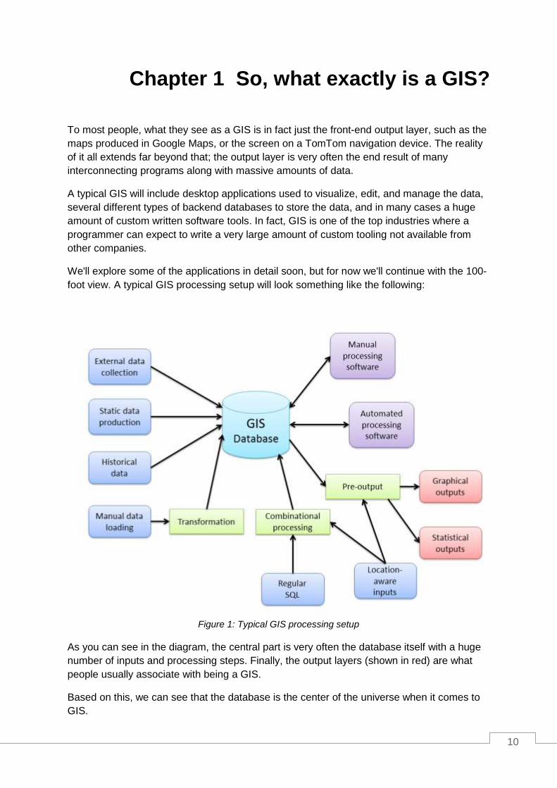
We'll explore some of the applications in detail soon, but for now we'll continue with the 100-
foot view. A typical GIS processing setup will look something like the following:
Figure 1: Typical GIS processing setup
As you can see in the diagram, the central part is very often the database itself with a huge
number of inputs and processing steps. Finally, the output layers (shown in red) are what
people usually associate with being a GIS.
Based on this, we can see that the database is the center of the universe when it comes to
GIS.
11
A Breakdown of the Components
Looking at the diagram in Figure 1, we can see that there are a number of parts that have
specific meanings. We have our inputs (blue), outputs (red), in-place processing (green),
and end processing (purple). At this point you might be asking yourself, "How is this different
from any other data-centric system I deal with?" and you'd be right to do so. The main
difference here is that in a typical GIS, you have to design everything in each component
from the very beginning. With a regular data-centric system, many of the components are
often optional or are combined into multifunctional components.
For a typical GIS, none of what you see in Figure 1 is optional, except for possibly your
inputs. Even then, the components you'll most likely see omitted are manual and historical
data.
So what do these separate entities entail, and why are they often not optional?
External Data Collection
As the name suggests, this is the process of gathering external data specific to the system
being designed. Typically this will come from custom devices running custom software (often
embedded or small scale) designed to create input data in a very specific form for the
system it is being used in. The lack of any in-place processing generally means the data
produced is in a format that is already acceptable in the setup.
This component is typically satisfied by many diverse pieces of technology, and in most
cases requires some training to use correctly. You'll often see things like digital surveying
equipment or specialized GPS devices fitted to vehicles, which in many cases will often feed
data back in real time using some kind of radio connection.
Static Data Production
Like external data, this process normally gathers data in a specific format for the system it is
being used in. Unlike external data however, you will generally find that static data is
produced in-house by scanning existing paper maps or digitizing features from existing
building plans, for instance.
Like external inputs, static data is often produced using custom software and processes
specific to the business.
Historical Data
Because of the size and amount of data produced in a typical GIS setup, there is often a
need to back up data into a separate archival system while still maintaining the ability to
work with it if needed. Often, data of this nature is created by planning authorities showing
things like land use over time or recording where specific points of interest are. This is
treated as a separate input because the data is usually read only, and similarly to external
and static data, was at one time produced specifically for the system.
12
Manual Data Loading
While the name of this type of input may suggest the same as external data, the actual data
obtained in this step is usually very different. Data coming into the system via this input will
often be in the form of pre-provided data from a GIS data provider. In the United Kingdom,
this will often mean data provided by companies like Ordnance Survey. In the United States,
this might mean data provided by institutions such as the U.S. Geological Survey or TIGER
data from the U.S. Census Bureau.
At this step, wherever data is obtained from, it's almost guaranteed that it will need to be
transformed into a format that is useable in the GIS it's destined for. More often than not, it
will need to go through some kind of in-place process before it's useable in any way.
Regular SQL Queries
Since most GIS have a large database at the center of them, SQL still plays an important
role and probably always will. However, in GIS terms, these queries not only involve the
normal SQL that you're used to seeing in a database management system, but also
geospatial SQL. We'll cover GIS-specific SQL a little later on; for now, inputs here are
usually generated from things like search queries.
As an example, when you type the name of a place or a ZIP code into Google, Bing, or
Yahoo Maps, the web application you're looking at will most likely turn your search into a
query that uses geospatial SQL to examine data in the core database. This, in turn, will be
combined with other processes to produce an output, which in this case will usually be a
map displaying the location you searched for. Another example might be an operator in an
emergency services control room entering the location of an incident, and combining that
with the known locations of nearby emergency vehicles to aid in making a decision as to
which vehicle to send to the incident.
Location-Aware Inputs
The last input type is probably the one that is familiar to most people. Location-aware data
most often comes from the GPS input on a mobile phone or other GPS-enabled device. It is
generally common latitude and longitude information. We'll cover this more when discussing
NMEA data.
Graphical Outputs
Now we move to the output layers, the first of which is the graphical one and what most
people are familiar with. Output data here is very often in the form of a raster-based map
with all operations performed to produce a single output tile in the form of a standard bitmap
(such as a .jpeg). However, far more is involved than simple map tiles. Graphical outputs
can, and very often are, produced in various vector formats, or as things like AutoCAD
drawings for loading into a CAD or modeling package. In fact, even in web environments
where people are used to seeing bitmap tiles, it's common for graphical output to take the
form of SVG or KML data combined with a custom Google Maps object. Raster tiles are just
the tip of the iceberg.

13
Statistical Outputs
Outputs in this group are the complete opposite of graphical outputs. Data is often the by-
product of several GIS–SQL operations based on the input data and processes going on
within the system. Just like general database data, from this output you'll get facts and
figures that can be used to report statistics to management or marketing teams. The reason
we treat this separately, however, is because of the nature of the information.
While you might be tempted to just say, "It's only numbers," in some cases it's numbers that
have no meaning unless there is some GIS input involved. As an example, let's say we have
a number of geographic areas representing plots of land, and with each of those areas we
have a monetary value for that plot.
We can easily say, "Give me the values of each plot in descending order," enabling you to
see which is the most expensive piece of land overall. This is where the difference stops,
however. Let's say we now know that all land in a district has a 1% tax for every square
meter a plot consumes. We know by looking at a graphical output of the map that the
visually bigger areas are going to be more expensive, but you can't convey that to a
computer.
You can, however, ask using GIS–SQL for a statistical analysis based on a percentage of
the land's plot value multiplied by however many square meters are in the defined area
boundary.
Manual Processing Software
Anything in the system that requires an operator and some software to make changes falls
under the category of manual processing software. Typically, this is both an input and an
output because in most cases this involves changes being made to the underlying data
manually.
This is usually the area where you'll see large GIS packages such as ESRI, DigitalGlobe,
and MapInfo used. We'll cover some of these later. An example of what might be performed
at this stage is boundary editing. Let's say that you added some town boundaries as area
definitions several years ago, and since they were first added the towns have increased in
size. You would then find a GIS expert who, with his or her chosen software and some
satellite imagery, would edit your boundary data so that its definition better fits the newly
expanded imagery.
Automatic Processing Software
Operations running at this stage are generally not much different than those being run
manually. The reason we see a clear separation is because some processes simply cannot
be automated and need a human eye to pick out details. Going back to our previous
example of the town boundaries, it's not beyond imagination that a process can be defined
to analyze an aerial image and determine if boundaries need to be removed.

14
Most often, however, automatic editing is used to perform tasks such as drift correction or
height and contour changes due to earth movement.
Transformation Tasks
As mentioned in the discussion of manual data input, when obtaining data for incorporation
into a GIS, the data will rarely be in a format suitable for inclusion in the system.
Making the data usable may involve something as simple as a coordinate transform, or
something as complex as combining multiple datasets based on common attributes and
more. Transformation processes can and often do seriously affect the overall data quality,
and many systems can end up with a lot of deeply rooted problems caused by mistakes
when transforming data.
In the U.K., these processes are almost always seen when working with latitude and
longitude coordinates, as nearly all the data supplied by U.K. authorities will be in meters
from the origin, rather than degrees around the center.
Combinational Processing
Combinational processing is generally in-place processing that is the result of various input
operations. It's not too different from using a join in a regular database operation. The result
is a combination of processes and input data steps that ultimately work in real time to
produce a defined input data set.
Pre-Output
Last but not least is the pre-output step. As the name suggests, this is the final processing
required before the output is useable. A pre-output process may include transforming an
internal coordinate system to a more global one; for example, U.K. meters back to a global
scale, or converting a batch of statistics to a different range of values. Location-aware inputs
are often included in this step, typically in a navigation system. For example, a location's
graphical representation could be combined with current mapping to produce a visual output
for a tracking map.
The Database
So just what makes a GIS database so different from a normal database? Honestly, not
much. A GIS database is simply specialized for a particular task.
A better way to illustrate what makes a GIS database unique is to look at the growing world
of big data. These days, it's hard not to notice how much noise is being made by NoSQL and
document-centric database providers. These new-breed databases fundamentally do the
same things as a normal database, but use specialized processes that perform particular
operations in better, more efficient ways.

15
Looking at a GIS database through the lens of a non-GIS connection, the geometric data is
nothing more than a custom binary field, or blob, that the software and processes working
with the system know how to interpret. In fact, it's possible to take a normal database engine
and write your own routines, either in the database or in external code, to perform all of the
usual operations you would expect but with GIS data.
In general, when a database is spatially enabled, it will have much more than just the ability
to understand the binary data added to it. There will be extensions to the SQL language for
performing specialized GIS data operations, new types of indexes to help accelerate
lookups, and various new tables used to manage metadata pertaining to the various types of
GIS data you may need to store.
I'm not going to list every available operation in this book, only the most important things you
need to know to get started. At last count, however, there are more than 300 different
functions in the last published OGC standards.
OGC What?
The OGC standards are the recommendations set by the Open Geospatial Consortium.
They define a common API, a minimum set of GIS–SQL extensions, and other related
objects that any GIS-enabled database must implement to be classified as OGC compliant.
Because of the diversity of GIS and their data, these standards are rigorously enforced. This
enables nearly every bit of GIS-enabled software on the planet to talk to any GIS-enabled
database and vice versa using a common language.
Note that when selecting a database to use, there are many that claim to be spatially aware
but are not OGC compliant. Prime examples are MS SQL and MySQL.
In general, MS SQL features the OGC-ratified minimum GIS–SQL and functional
implementation, but its calling pattern varies significantly from most GIS software. MS SQL
also features changes to column names in some of the metadata tables, which means most
standard GIS software cannot talk to a MS SQL server. Note also that MS SQL didn't add
any kind of GIS extensibility until 2008, and even in the newer 2008 R2 and 2012 versions,
the GIS side of things is still not completely OGC compliant.
MySQL has similar restrictions, but also treats a number of core data types very differently,
often leading to rounding errors and other anomalies when performing coordinate
conversions. You can find the full list of OGC standards documents on the OCG website at
http://www.opengeospatial.org/standards/is.
A good place to look for information comparing various databases is on the BostonGIS
website at
http://www.bostongis.com/?content_name=sqlserver2008r2_oracle11gr2_postgis15_compar
e#221.
There are also a number of other good starter articles on the site. The downside is that the
site is cluttered and sometimes very hard to read.

16
The Metadata Tables
All OGC-compliant GIS databases must support two core metadata tables called
geometry_columns and spatial_ref_sys. Most GIS-enabled software will use the existence
of these tables to determine if it is talking to a genuine GIS database system. If these tables
don't exist, the software will often exit.
A good example of this was with early versions of MySQL where the table names were
reserved by the database engine, but did not physically exist as tables. This would cause the
MapInfo application to attempt to create the missing tables, but it would receive an error on
trying doing so, thus preventing the database from being used correctly by the software.
The geometry_columns table is used to record which table columns in your database
contain geospatial data along with their data type, coordinate system, dimensions, and a few
other items of related information.
The spatial_ref_sys table holds a list of known spatial reference systems, or coordinate
systems as they may be better known. These coordinate systems are what define
geographic locations in any GIS database; they are the glue that allows all the functionality
to work together flawlessly, even with data that may have come from different sources or
been recorded using different geographic coordinate systems.
The entries in the spatial_ref_sys table are indexed by a number known as the EPSG ID.
The EPSG, or European Petroleum Survey Group, is a working group of energy suppliers
from the oil and gas industry who confronted a common problem that arose when surveying
the world's oceans for oil reserves: positioning on a global scale. Some companies used one
scale, others used a different scale; some used a global coordinate system, while others
used a local one.
The group's solution was to record the differences between each scale and the information
required to convert from one scale to another reliably without any loss of precision.
Today, every GIS database that claims to be OGC compliant includes a copy of this table to
ensure that data conversions from one system to another are performed with as much
accuracy as possible.
We'll cover the actual coordinate systems a little later in the book. For now, all you really
need to be aware of is that if the spatial_ref_sys table does not exist or has no data in it,
you will be unable to accurately map or make real-world translations of any data you
possess.
Also note that it is possible to save space by removing unnecessary entries from this table. If
your data only ever uses two or three different coordinate systems, it's perfectly acceptable
to remove the rest of the entries to reduce the size of the table. This can be especially useful
when working with mobile devices.
If you only work with data in your own range of values, arguably there can be no data in the
spatial_ref_sys table at all. I would, however, caution you against removing the table
entirely. As previously mentioned, most GIS software will look for the presence of this and
the geometry_columns table to signify the existence of a GIS-enabled database.

17
What's Actually in the Metadata Tables?
The geometry_columns table holds data pertaining to your data and has the following
fields:
f_table_catalog The database name the table is defined in.
f_table_schema The schema space the table is defined in.
f_table_name The name of the table holding the data.
f_geometry_column The name of the column holding the actual data.
coord_dimension The coordinate dimension.
srid The spatial reference ID of the coordinate system in use.
type The type of geometry data stored in this table.
The catalog, schema, and name fields are used in different ways by different databases.
Oracle Spatial, for example, has a single geometry_columns table used for the entire
server, so the catalog field is used to name the actual database. Postgres, however, stores
one geometry_columns table per database, so the catalog field will usually be empty. On
the other hand, the schema field is used in both Postgres and MS SQL. In Postgres, the
field is usually set to public, whereas in MS SQL it's normally set to dbo for the publicly
accessible table set.
The table name and column name are pretty self-explanatory. The coordinate dimension in
most cases will be 2, meaning that the coordinate system has only x-coordinates and y-
coordinates. Postgres and Oracle Spatial do have 3-D capabilities, but I've yet to see them
used very much outside of very specific circumstances, and I've never seen a
coord_dimension field set to anything other than 2.
We'll cover the srid field in just a moment. The type, however, needs further explanation.
Database Geometry Types
Any OGC-compliant database has to be able to store three different types of primitives. They
are:
point
line
polygon
18
The names themselves are fairly explanatory. A point is a single x, y location. A line is a
single segment connected by two x, y end points. A polygon is an enclosed area where a
number of x, y points form a closed perimeter.
However, the three base types are not the only geometry types you'll work with. There are
variations such as:
linestring
multilinestring
multipolygon
Plus a few others that are rarely used.
A linestring can be thought of as a collection of line objects where each point, except for the
start and end points, is the same as the start or end point of the adjacent line. For example:
1,2 2,3 3,4
would be a linestring that starts at 1,2, goes through two segments, and ends at 3,4.
A multilinestring can be thought of as a collection of linestrings. For example:
(1,2 2,3 3,4) (6,7 7,8 8,9)
would be two linestrings running from 1,2 to 3,4, and from 6,7 to 8,9, each consisting of two
segments. The two linestrings would have a gap between them.
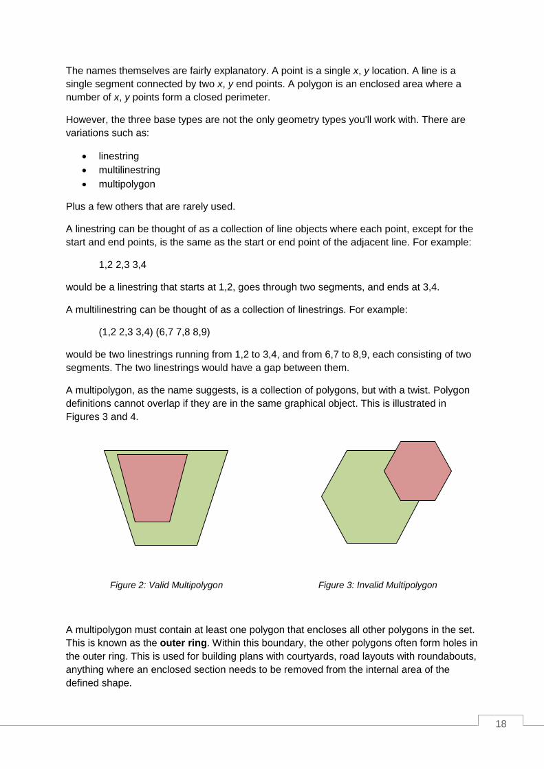
A multipolygon, as the name suggests, is a collection of polygons, but with a twist. Polygon
definitions cannot overlap if they are in the same graphical object. This is illustrated in
Figures 3 and 4.
Figure 2: Valid Multipolygon Figure 3: Invalid Multipolygon
A multipolygon must contain at least one polygon that encloses all other polygons in the set.
This is known as the outer ring. Within this boundary, the other polygons often form holes in
the outer ring. This is used for building plans with courtyards, road layouts with roundabouts,
anything where an enclosed section needs to be removed from the internal area of the
defined shape.

19
Many spatial databases, however, will define even single polygons as multipolygons. This is
done so that it's easy to insert cutouts if needed at a later time.
What Types Should I Use for My Data?
The data types you use depend what your data is representing. If you have a series of
locations representing shops, you'll most likely just want to define those as points. If, on the
other hand, your data represents roads between those points, a multilinestring is probably a
better choice. If you want to mark the building outlines of each shop, you'll want to use a
polygon or multipolygon depending on the complexity of the structure.
There are no hard and fast rules for data types. You only have to keep in mind that if you
don't use a data type appropriate for the operations you expect to perform, you're almost
certain to end up with errors in any calculations you do.
Think back to our shops. If you're searching for the largest one, you need to test for area,
and you can't test for area using a single point. On the other hand, if all you want to do is
provide a searchable map for a customer to find his or her closest shop, you don't need to
store more data than you need, so a simple point will do.
Enough of data layout for now. We'll come back to it in a while. Let's continue with the
metadata tables.
Metadata Tables, Part 2
As mentioned previously, the spatial_ref_sys metadata table holds conversion data to allow
conversions from one coordinate system to another.
Each entry in this table contains specific information such as units of measurement, where
the origin is located, and even the starting offset of a measurement.
Most of us are familiar with seeing a coordinate pair such as this:
54.852726, -1.832299
If you have a GPS built into your mobile phone, fire it up and watch the display. You'll see
something similar to this coordinate pair. Note that on some devices and apps, the
coordinates may be swapped.
This coordinate pair is known as latitude and longitude. The first number, latitude, is the
degrees north or south from the equator with north being positive and south being negative.
The second number, longitude, is the degrees east or west of the Prime Meridian with west
being negative and east being positive. The correct geospatial name for this coordinate
system is WGS84. Its SRID number is 4326 in the spatial_ref_sys table.
We'll come back to the different coordinate systems and why they exist in just a moment. For
now, let's continue with the description of the spatial reference table. The spatial_ref_sys
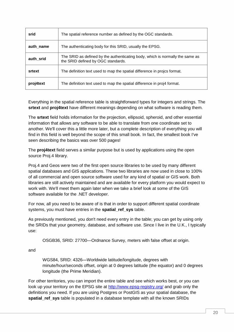
table has the following fields:
20
srid The spatial reference number as defined by the OGC standards.
auth_name The authenticating body for this SRID, usually the EPSG.
auth_srid The SRID as defined by the authenticating body, which is normally the same as the SRID defined by OGC standards.
srtext The definition text used to map the spatial difference in projcs format.
proj4text The definition text used to map the spatial difference in proj4 format.
Everything in the spatial reference table is straightforward types for integers and strings. The
srtext and proj4text have different meanings depending on what software is reading them.
The srtext field holds information for the projection, ellipsoid, spheroid, and other essential
information that allows any software to be able to translate from one coordinate set to
another. We'll cover this a little more later, but a complete description of everything you will
find in this field is well beyond the scope of this small book. In fact, the smallest book I've
seen describing the basics was over 500 pages!
The proj4text field serves a similar purpose but is used by applications using the open
source Proj.4 library.
Proj.4 and Geos were two of the first open source libraries to be used by many different
spatial databases and GIS applications. These two libraries are now used in close to 100%
of all commercial and open source software used for any kind of spatial or GIS work. Both
libraries are still actively maintained and are available for every platform you would expect to
work with. We'll meet them again later when we take a brief look at some of the GIS
software available for the .NET developer.
For now, all you need to be aware of is that in order to support different spatial coordinate
systems, you must have entries in the spatial_ref_sys table.
As previously mentioned, you don't need every entry in the table; you can get by using only
the SRIDs that your geometry, database, and software use. Since I live in the U.K., I typically
use:
OSGB36, SRID: 27700—Ordnance Survey, meters with false offset at origin.
and
WGS84, SRID: 4326—Worldwide latitude/longitude, degrees with
minute/hour/seconds offset, origin at 0 degrees latitude (the equator) and 0 degrees
longitude (the Prime Meridian).
For other territories, you can import the entire table and see which works best, or you can
look up your territory on the EPSG site at http://www.epsg-registry.org/ and grab only the
definitions you need. If you are using Postgres or PostGIS as your spatial database, the
spatial_ref_sys table is populated in a database template with all the known SRIDs

21
available when you install the database. Creating your own databases is simply a matter of
using this template to have a fully populated table from the start.
One note of caution before we move on: some databases, while they do support the
geometry_columns and spatial_sys_ref metadata tables, don't create them by default. MS
SQL 2008 is noted for this; it uses its own methods for storing spatial metadata. You may
find that in some cases you will be required to create some of these tables manually before
you can use your database. Additionally, you may also find that some databases create the
tables but use a slightly different naming convention, especially for the geometry_columns
table. For this reason, it's always better to use the official OGC-compliant spatial SQL
command set (which can be downloaded from http://www.opengeospatial.org/standards/sfs)
to manipulate the data in these tables, rather than trying to manipulate the entries directly.
Coordinate and Spatial Location Systems
Before we can get onto the technical fun stuff and start to play, we have to cover a little more
theory. You must understand why all these different SRIDs and coordinate systems exist.
I'd like to send you merrily on your way into your first GIS adventure right now and say this
stuff really doesn't matter; however, the truth is I can't and it does matter. In fact, it matters a
great deal.
If you don't comprehend this coordinate stuff correctly, it's possible to map an automobile's
track as being in the middle of the Atlantic Ocean. While this may not matter for the
application you're working on—you may be looking at a general overview of customer
dispersal, for example—you should still try to make sure your application is as accurate as it
can possibly be.
So the answer to the million-dollar question, "Why do we have to deal with all this coordinate
stuff?" boils down to one thing, and one thing only:
The Earth is not flat.
There, I said it. And all naysayers out there who still believe it is need to build themselves a
top-notch GIS and check it out.
Jokes aside though, it's the fact that our planet is a sphere that causes all these coordinate
system headaches. To make matters even worse, our humble home is not even a perfectly
round sphere. It's slightly elongated around its axis, a little like a rugby ball, but not quite as
pronounced. This causes further complications because the math we need to use as we look
at positions closer to the poles must compensate for the differences in the Earth's curvature.
Degrees, Minutes, and GPS
Okay, so how exactly do we deal with this curvature? There MUST be one measurement
that makes sense throughout the whole globe, right? If not, then how on Earth do airplanes

22
and ships navigate from country to country without getting lost or having to keep track all of
these different SRIDs?
You'll be pleased to know there is, but it's not as straightforward as just mapping an x
position and a y position at a certain place on the globe.
If you look at any geography textbook or world map, you'll see the Earth is divided into
rectangles. These rectangles are formed from the lines of latitude and longitude that make
up our planet's wireframe model. It looks something like the following:
Figure 4: Earth's wireframe model
Each horizontal and vertical line represents one or more whole degrees depending on the
scale factor being used. Minutes are then used to offset the position within that grid square.
When we express a latitude of 50° 25' 32" N, what we are actually saying is 50 degrees
latitude, plus 25 minutes and 32 seconds north into that square, in simple terms. There's a
little more complexity to it if truth be told, but unless you're navigating the high seas or
piloting a commercial airliner, you're probably not going to need to go into that much detail.
The same works for longitude. Everything is expressed as a positive number, so west of the
Prime Meridian is suffixed with a W, and everything to the east is suffixed with an E.
Combining these with the north and south longitude designations divide the planet into four
quadrants of 180 degrees each.
How is this of any relevance to the GIS developer?
If you're looking to retrieve the data from any commercial-grade GPS, particularly those built
into mobile phones, you'll almost always come face to face with the National Marine
Electronics Association and its standards for electronic navigation devices to communicate,
known as the NMEA 0183 standard. Opening the GPS port on just about any device will
produce a constant stream of data that looks very similar to the following:
$GPGGA,092750.000,5321.5802,N,00630.3372,W,1,8,1.03,61.7,M,55.2,M,,*76
$GPGSA,A,3,10,07,05,02,29,04,08,13,,,,,1.72,1.03,1.38*0A
$GPGSV,3,1,11,10,63,137,17,07,61,098,15,05,59,290,20,08,54,157,30*70
$GPGSV,3,2,11,02,39,223,19,13,28,070,17,26,23,252,,04,14,186,14*79
This data stream is the navigation data emitted by the GPS circuitry in the device in
response to what it's able to receive from the GPS network orbiting the Earth. We'll come
23
back to this in more detail in a later chapter. For now, I'd like to draw your attention to the
first line of this data, specifically the following entries:
5321.5802,N and 00630.3372,W
These are the GPS' current location expressed as degrees and minutes. Deciphering them
is not hard once you get used to it, but it can be a little strange at first.
The format of the string is DDMM.mmmm for the latitude (vertical) direction and
DDDMM.mmmm for the longitude (horizontal) direction.
Starting with the north (latitude) measurement in the string, the first two digits are the
number of degrees, and the remaining numbers are the minutes. The numbers after the
decimal point are fractions of a minute. This gives us:
53 degrees, 21.5802 minutes north
For the longitude measurement, the first three digits are the number of degrees, and the
remaining digits are the minutes. All the numbers after the decimal are fractions of a minute.
This gives us:
6 Degrees, 30.3372 minutes west
Because this data is string data, it's essentially an exercise in cutting the string at specific
points to derive the values you want. Once you have them, the math to convert them to the
more familiar latitude and longitude (if you remember that was WGS84) format is very
simple.
First, you need to separate the first two digits from the latitude string and the first three from
the longitude. This gives us the following:
53 and 21.5802 for the north direction
006 and 30.3372 for west
Because there are 60 minutes in a degree, we must divide the minutes digits by sixty to find
what fraction of a degree they are, and then combine them with our whole degrees. So, for
our latitude:
53 + (21.5812/60) will give you 53.359686 degrees.
And for our longitude:
6 + (30.3372/60) will give you 6.505620 degrees.
You get simple positions from the numbers. To finish the conversion, you need to apply the
north and west directions as positive or negative numbers. The easiest way to manage
which directions are positive or negative is to change any west or south measurements to
negative. So with our numbers, the final coordinates in WGS84 latitude and longitude are:
53.359686, -6.505620

24
WGS84 is a global coordinate system standard, and while it is widely used, using it for
everything can cause some problems. Because WGS84 is designed to cover the globe, it's
designed also to be very lenient with the curvature of the planet. Think back to the wireframe
globe in Figure 4. Notice the shape of the rectangles as they near the top of the globe.
You can see in the diagram that the rectangles become longer and narrower. This stretching
also has to be accounted for in the coordinate system. Over long distances, it can cause
rounding and deviations to occur in your data.
If you're dealing with a territory where you only have a defined area of operation, using a
coordinate system more suited to that area is the preferred way of working. As I mentioned
previously, for me here in the U.K. it's often better for me to convert these WGS84
coordinates to OSGB36 before storing them in my database. As we'll see later when we start
looking at spatial SQL, your GIS database can do this on the fly when set up correctly.
That's pretty much all you need to know as a developer. There's much deeper stuff you can
dig into such as spheroid and airy calculations, geodetic measurements, and a lot of that
trigonometry stuff from school. The fact is that your GIS database and many of the tools
you'll use will actually do the vast majority of the heavy lifting for you. So while having a good
knowledge of the actual formulas used by the systems and the Proj.4 strings may be
interesting, I assure you of one thing: it will end up giving you a brain ache.
In the next chapter, we start to move onto more interesting things, starting with the software
we'll be using.
25
Chapter 2 The Software
Having a well-designed GIS database is great, but what software do you need aside from
that?
Unless you're doing everything from scratch, you'll need some kind of editing application,
some way to load your data, and most likely some kind of real-time data too.
The major problem is expense. You will quickly find that GIS software is probably one of the
most expensive software markets on the planet. Dollar for dollar, the overall cost for most of
these applications vastly outweighs your typical yearly operating system site license costs
for a small office—often for just one user in one app for 6 months.
Fortunately for us, there is also a huge open source and free software movement around
GIS mostly operated and managed by the Open Source Geospatial Foundation (OSGeo).
The OSGeo website at www.osgeo.org is the main hub for finding links to all the open
source and spatial tools available in the market today, as well as many links to tutorials,
news, and paid-for providers. They are a sponsor funded organization, and rely on groups
using the software to improve it and feed it back into system.
For those companies that don't like open source and require service and support contracts,
many of the open source offerings available do have such packages available for a small
cost.
Let's look at some of the choices available.
Database Software
Postgres and PostGIS
This combination is to the open-source GIS scene what the godfather is to the mafia. It's the
granddaddy of all GIS databases. It's fully OGC compliant, absolutely rock solid, time tested,
and is supported by every bit of GIS software on the planet.
Those who know their databases will know that Postgres has been around for a very long
time. It was originally a University of California, Berkley product started in 1986 by a
computer science professor named Michael Stonebraker. In 1995, two of Stonebraker's
students extended Postgres to SQL, and in 1996 their innovation left the classroom for the
world of open source.
Refractions Research realized that Postgres had enormous potential, and in 2001 set about
making an open source add-on for servers to give them full geographic and spatial

26
capabilities, ultimately producing PostGIS. From there, it's grown into a top-class database
system for enterprise and shows no signs of slowing down.
MySQL
Originally developed as a simple-to-use open source database from the beginning, MySQL
has included basic geometry types since at least v3.23. They may have been present earlier,
but there is no documentation for them prior to 3.23, and no mention of them in the history of
the database.
Version 3.23 documentation clearly states that the database is not fully OGC compliant. In
particular, the geometry_columns metadata table is not supported, and many of the
standard functions are renamed to be prefixed with a G—GLength, for example, so as not to
cause issues with the standard Length function. The level of support for GIS across different
versions of MySQL is questionable.
In more recent versions—I'm reading the version 5.6 documentation as I type this—the core
engine does seem to be more OGC compliant, and I certainly know of people who use it as
the central component in some complex GIS. Given that this is one of the few systems that
ships with support for GIS operations, there's no need to install third-party components to
spatially enable it.
MySQL is a very capable and fast system. It's also incredibly easy to administrate and has
enormous support in the community despite having been recently acquired by Oracle as part
of its buyout of Sun Microsystems. Its future is still a little uncertain, but one thing is sure: it
will remain at the center of most LAMP and WAMP open source web stack installations for
some time to come. You can learn more about MySQL at www.mysql.com.
SQL Server
Since this book is intended for .NET and Microsoft developers, I'm not going to delve into
SQL Server too much as most readers will know a lot of the capabilities of the system
already.
GIS functionality in the core product is a relatively new thing that was not fully introduced
until SQL Server 2008. Prior to this, there were a few unofficial third party add-ons that
spatially enabled SQL Server 2003 and SQL Server 2005, but these never really delivered. I
remember trying an add-on for SQL Server 2005 that repeatedly crashed the server only
when certain functions were called!
Even though SQL Server 2008 has GIS functionality baked in, it is probably the most non-
OGC compliant OGC compliancy I've seen in any product.
Let me explain: SQL Server 2008 implements all the functionality required in the OGC
specifications, functions such as ST_GeomFromText or ST_Polygonize and so on. But
because SQL Server is a CLR-based assembly, it doesn't allow functions to be accessed in
the same way. I'll discuss the SQL more in-depth later; for now, consider the following:
Standard OGC-compliant SQL

27
SQL Server 2008 OGC-compliant SQL
This minor difference causes all sorts of issues. In particular, it means that any software
using SQL Server 2008 as its backend needs specialized data adapters (usually based
around ODBC) to translate calls to the server in an OGC-compliant way. In fact, most GIS
software has only just recently started to provide built-in support via ODBC.
One positive aspect for .NET developers using SQL Server is direct support in .NET via the
Entity Framework and its Geometry and Spatial classes. If you’re working solely on the
.NET platform, there is a strong argument for not needing to use anything other than SQL
Server. If, however, you need access to GIS in general and the underlying SQL to
manipulate it, SQL Server is not the best choice.
The official SQL Server website is www.microsoft.com/sqlserver/en/us/default.aspx.
SQLite and SpatiaLite
SQLite is not strictly a database server, but one of the new generation single-file database
engines designed to be embedded directly into your application. SQLite has amazing
support on a massive number of platforms, and is possibly one of the most cross-platform
kits I've had the pleasure to use.
Compared to the big three already mentioned, SQLite is a relative newcomer to the scene,
but it runs remarkably well and is incredibly efficient, especially on mobile platforms. In fact,
it's so good on mobile platforms that it's been chosen as the database engine of choice on
Android devices and Apple's iOS, as well as featuring full support on Windows Phone
through the use of a fully managed .NET interface.
SpatiaLite, the spatial extension for the SQLite engine, is not so lucky. Its sources are
available, but built binaries are only provided for the Windows platform. For any other
platform you'll need to download the source and then port it to your platform of choice. While
this is not difficult, the sources are all in standard ANSI C and can be a little tricky to get
working, especially if you have very little native C or C++ experience.
There are binary builds available for platforms other than Windows, but these are very
fragmented and often out of date. Bear in mind also that SpatiaLite, like much of the open
source GIS-based software available, depends on Proj.4, GEOS, and other libraries to
provide many of its advanced features. If you have to custom build SpatiaLite for your
platform, you'll likely have to custom build the dependent libraries as well.
SELECT id,name,ST_AsText(geometry) FROM myspatialtable
SELECT id,name,geometry.astext() FROM myspatialtable

28
Does this put SQLite and SpatiaLite out of the picture? Not really. I have yet to find anything
else that works on so many different mobile platforms with such a consistent API. While
there is some work involved, building for your platform is quite simple in most cases, and
certainly no more complex than the work that needs to be performed when installing
Postgres/PostGIS, MySQL, or SQL Server. However, unless you need spatial capabilities
that are universally mobile, SQLite and SpatiaLite are probably not worth the effort.
The SQLite website is sqlite.org. Its .NET interface is available at
http://system.data.sqlite.org/index.html/doc/trunk/www/index.wiki.
The SpatiaLite website can be found at www.gaia-gis.it/gaia-sins/index.html.
Oracle Spatial
Unless you're a multimillion dollar enterprise, it's very unlikely you are going to have access
to Oracle Spatial. Oracle Spatial is to the commercial world what Postgres is to the open
source world.
It's big, it's hungry, it costs an arm and a leg to license, and the learning curve is probably
steeper than climbing Mount Everest.
Many government agencies in the U.K. use it for their mapping and planning work, and
larger companies such as oil and gas giants deploy multibillion-dollar infrastructures based
around it to support their survey work. If you're in a position where you are using this, then
you most likely won't be talking to the system directly; you'll already have software set up for
you that manages everything the database can do. Systems built around Oracle are
generally designed specifically by Oracle's consultants for a specific purpose, and have an
entire toolkit built around them at the same time. Most of the software I mention in this book
does not—to the best of my knowledge—have the ability to connect to Oracle Spatial; or if it
does, the setup and operation of doing so is tremendously complex.
The official Oracle Spatial website can be found at
www.oracle.com/us/products/database/options/spatial/overview/index.html.
What about the rest?
There are many more database packages available out there. Some support GIS out of the
box, and some don't. Some of them need third-party add-ons or involve a complicated setup.
The reason for leaving others out is because there is simply not enough room in this book. If
you decide to explore additional databases, you may want to check out the following:
MongoDB at www.mongodb.org
SpaceBase at paralleluniverse.co
CouchDB at couchdb.apache.org
CartoDB at cartodb.com
SpaceBase in particular looks like it could be a lot of fun. Its primary goal is to track and
store online MMO-based game characters and assets in a near real-time 3-D world for
multiplayer games.

29
GIS Desktop Software
In order to manipulate your GIS assets you need a good desktop application—preferably
one that not only allows you to view and manipulate your data, but also allows you to import
and export data with relative ease.
The latter point is also important because the sole purpose of some applications is to move
data into and out of your system, and other applications are made only for viewing data.
Applications for moving data are commonly known as ETL (Extract, Transform, and Load)
packages. ETL packages are available for many database engines in general, not just for
those designed to manipulate geospatial data.
Fortunately, most software allows you to do both. Starting with these packages, here are
some of the more well-known ones:
ESRI ArcGIS
One of the big players in the market, ESRI, has been providing GIS and mapping software
now for over 20 years. The software is like many GIS packages: quite expensive, and
certainly outside the price range for most hobbyists and small and medium enterprises. ESRI
does, however, offer a free product called ArcGIS Explorer Desktop that can be used to
make basic maps and produce your own mapping data.
One thing to note about ArcGIS Explorer Desktop is that it can be used to look at imagery
from Bing's and Google's mapping services. As you can see in the following screenshot, I've
marked some features in the City Centre of Newcastle-upon-Tyne, England:
Figure 5: A Modified Existing Map in ArcGIS Explorer Desktop
You can find out more about ArcGIS Desktop Explorer and other ESRI software at
www.esri.com/software/arcgis/explorer.

30
Pitney Bowes MapInfo
MapInfo, like the ESRI suite, is a large commercial package designed with the enterprise in
mind. I know from my own experience that it's used by a lot of utilities companies such as
mobile phone operators for managing their network map assets. Like Oracle Spatial, you'll
rarely come across this package unless you have a very specialized management system
for your geospatial data.
While it can load and work with all the common map formats and services like Bing, Google,
and others, MapInfo's primary design is to handle non-standard data in large, heavily
customized GIS databases. Its strength lies in its ability to be extended using its own
programming language called MapBasic that is often deployed in many custom
configurations. For instance, it may be deployed in a wireless service's operator consoles for
showing where network faults are located, or at a delivery service for keeping track of its
vehicles.
You can find more info about Pitney Bowes MapInfo at
www.pbsoftware.eu/uk/products/location-intelligence/.
OpenJUMP
Now we come to the first of the open source desktop offerings, OpenJUMP. Designed from
the start to be open source, it's built using the Java platform, and as expected can talk to
most of the GIS databases in use today.
It allows you to load and view your own spatial data, handle shapefiles and GML files, and
export maps as SVG for display on the web.
Its primary purpose is to edit mapping data in preparation for creating vector maps for web
use. I've personally never used OpenJUMP, but it seems like a very capable package for
creating web maps from scratch.
Figure 6: Using OpenJUMP

31
You can find more out about OpenJUMP at www.openjump.org.
Quantum GIS
There's nothing I can say that does Quantum GIS (QGIS) justice. This package can do just
about anything. It's on par with applications such as ESRI and MapInfo, fully open source,
and officially supported by the OSGeo Foundation.
The main application is written using Python, and as a result will run on Linux, Mac OS,
Windows, and anything else that supports Python in a desktop environment.
Now on version 1.8.0, the development of Quantum GIS has built strength upon strength in
the relatively short time it's been available. The extension API exposed by the system is
simply amazing, and can be customized at every level—from re-engineering the main UI, to
plug-ins that expose things like live GPS tracking, to the creation of brand new vector layers
by applying algorithms to different layers in a package.
It comes standard in OSGeo4W, a collection of open-source geospatial software for
Windows, along with Grass, MSYS, OpenEV, and many others. Backed by tools such as
GDAL, pg2mysql, and many others, the only limit I've found to this package is your
imagination.
Quantum is my desktop tool of choice when dealing with all the different types of data
available. It can handle Postgres and all other major databases with the same ease that it
imports and exports just about every known GIS file format on the planet.
It's also one of the few packages that can import and export Google Earth (KML) files for
direct use with projects that make use of Google's mapping API. The current version now
also includes a handy geospatial file explorer, which means you can browse and view your
local file system resources without needing to fire up the full-blown GUI.
In the following screenshot, you can see QGIS loaded with a multilayer vector map (an
Ordnance Survey Strategi map of the U.K.) zoomed in on Newcastle upon Tyne City Centre:
32
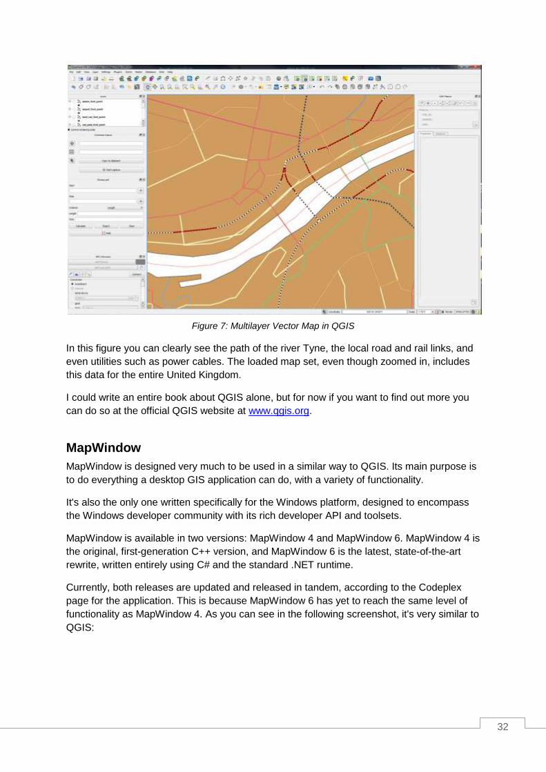
Figure 7: Multilayer Vector Map in QGIS
In this figure you can clearly see the path of the river Tyne, the local road and rail links, and
even utilities such as power cables. The loaded map set, even though zoomed in, includes
this data for the entire United Kingdom.
I could write an entire book about QGIS alone, but for now if you want to find out more you
can do so at the official QGIS website at www.qgis.org.
MapWindow
MapWindow is designed very much to be used in a similar way to QGIS. Its main purpose is
to do everything a desktop GIS application can do, with a variety of functionality.
It's also the only one written specifically for the Windows platform, designed to encompass
the Windows developer community with its rich developer API and toolsets.
MapWindow is available in two versions: MapWindow 4 and MapWindow 6. MapWindow 4 is
the original, first-generation C++ version, and MapWindow 6 is the latest, state-of-the-art
rewrite, written entirely using C# and the standard .NET runtime.
Currently, both releases are updated and released in tandem, according to the Codeplex
page for the application. This is because MapWindow 6 has yet to reach the same level of
functionality as MapWindow 4. As you can see in the following screenshot, it's very similar to
QGIS:
33
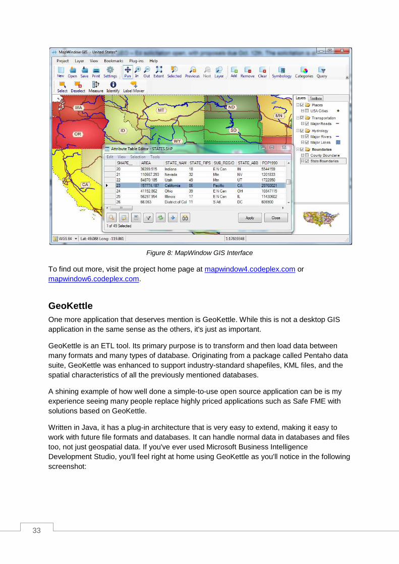
Figure 8: MapWindow GIS Interface
To find out more, visit the project home page at mapwindow4.codeplex.com or
mapwindow6.codeplex.com.
GeoKettle
One more application that deserves mention is GeoKettle. While this is not a desktop GIS
application in the same sense as the others, it's just as important.
GeoKettle is an ETL tool. Its primary purpose is to transform and then load data between
many formats and many types of database. Originating from a package called Pentaho data
suite, GeoKettle was enhanced to support industry-standard shapefiles, KML files, and the
spatial characteristics of all the previously mentioned databases.
A shining example of how well done a simple-to-use open source application can be is my
experience seeing many people replace highly priced applications such as Safe FME with
solutions based on GeoKettle.
Written in Java, it has a plug-in architecture that is very easy to extend, making it easy to
work with future file formats and databases. It can handle normal data in databases and files
too, not just geospatial data. If you've ever used Microsoft Business Intelligence
Development Studio, you'll feel right at home using GeoKettle as you'll notice in the following
screenshot:

34
Figure 9: GeoKettle Interface
If you want to find out more, you can visit the GeoKettle website at
www.spatialytics.org/projects/geokettle.
The Remaining Packages
As with database engines, there are simply too many GIS desktop packages for me to list
them all. Wikipedia has a good list of geospatial and GIS software, ranging from pricey to
free, at en.wikipedia.org/wiki/List_of_GIS_software, including those that I've covered here.
My two personal favorites are QGIS and GeoKettle, but I encourage you to try all that you
are able to. Over the years, I've used many desktop GIS packages; some have very steep
learning curves, and some you can pick up in less than five minutes. As with anything, you
should pick the tool that does the job you need to perform in the best and easiest way
possible.
Please also note that the applications I've listed are used predominantly in the U.K. and
Europe. The popularity of applications varies all over the world. For instance, I believe that
IDRISI is a popular package used in Canada. The applications listed in this section are the
ones I use in my day-to-day GIS work.
As I've already mentioned, you have a ton of other stuff to take care of besides your choice
of software.

35
Development Kits
Since this book is aimed at the .NET developer, it's only right that we include a section on
the kits available for using geospatial data in your own .NET applications.
We'll cover a few practical examples later on, but for now I'll list the kits I've used or seen in
use. Please note, however, that this is not an exhaustive list. The toolkits I describe are all
designed for use under .NET on the Windows platform. As I've mentioned, applications like
QGIS can be vastly extended, and there are many toolkits available under Linux and Mac
systems that I've not yet and likely won't cover. If you're starting a project where you know
you're going to be writing custom user interfaces, do your research beforehand. Instead of
writing them from scratch, there's every chance you can modify an existing application to suit
your needs.
MapWinGis
MapWinGis is the central GUI component behind MapWindow 4 and MapWindow 6. It's an
OCX control written in C++ that can be used in any language that supports OCX on the
Windows platform.
In the past, I used the original version of this component. It's been some time now since I've
done any development using it. As with many of these components, it has a permanent
home on Codeplex at mapwingis.codeplex.com.
It is designed to do most of the heavy lifting for you, leaving you free to concentrate on the
GUI aspects of your application. Please note that it's designed for use in desktop
applications, not web-based applications, and as far as I'm aware cannot be used in WPF or
Silverlight.
DotSpatial
DotSpatial is a sister project of the MapWindow stable, and actually forms most of the core
of the new MapWindow 6 .NET rewrite. DotSpatial also incorporates a few other Codeplex
projects under its hood too, most notably GPS.Net and GeoFramework. Both are still
available separately.
One thing that's worth noting about DotSpatial is that like QGIS, this toolkit has the backing
of the OSGeo Foundation. As part of its kit, it also has the entire open source GIS developer
library (including GEOS, Proj.4, GDAL, and many more) packaged as ready-to-use Windows
DLLs for direct inclusion in your projects.
The project home page can be found on Codeplex at dotspatial.codeplex.com/.
SharpMap
SharpMap is one of the older toolkits for .NET. It has been around a little longer than
DotSpatial.

36
It can handle most types of vector and raster data, including the NASA Blue Marble tile set
for the entire globe.
According to its documentation, the SharpMap library supports both desktop and web-based
projects (the later via the use of the AJAX Map control). It can also create custom thematic
map styles by combining many different types of overlay.
The project home page can be found at sharpmap.codeplex.com.
BruTile
While not a full GIS library in the same sense as others, BruTile does one thing, and does it
very well: it serves raster tiles cut up and reorganized on the fly to allow smooth scrolling and
zooming of any input that the library handles.
BruTile is actually used by both SharpMap and DotSpatial to provide output support on their
raster tile components. It's also used to display open street map data running inside a
Silverlight map at brutiledemo.appspot.com.
BruTile can be used in any type of project, from web and Silverlight, to high-end desktop
apps. It also has an adapter that allows it to be used in custom ArcGIS deployments.
The project home page is located at brutile.codeplex.com.
And There's More...
As with the other bits of software mentioned previously, there are simply many, many more
available. What I've not even begun to cover here is the fact that all the major players such
as ESRI and Pitney Bowes offer their own SDKs as well. In fact, a large chunk of ESRI's
profit comes from the provision of GUI toolkits that are used in much the same way as
MapWindow. Unfortunately, as much as I would like to, there are simply too many to cover in
this short book.
The Demos
So now we get to that all-important question: what will I be using for the demos in this book?
I already have a setup of PostgreSQL with PostGIS, and most of my spatial SQL examples
will be done using this. Any database management tool you have that can connect to
Postgres will work. However, I will be using the one that comes provided with the server:
pgAdmin.
In addition to this, I'll be using Quantum GIS to manage and display data along with a
demonstration of using GeoKettle to load some data.
For the programming examples, I'll be using SharpMap in Visual Studio 2010 Professional in
the C# language. The samples can be downloaded from bitbucket.org/syncfusion/gis-
succinctly.

37
Please note that I won't be covering how to install and initially set up any of these
applications. This is a fairly simple operation in most cases, and one that I'm going assume
the reader of the book is familiar with. If you have any issues with installing the software, all
the applications mentioned in this book have very active communities and help forums.
For those of you who are familiar with Stack Overflow, its GIS-specific site can be found at
gis.stackexchange.com.
Many of the regulars there are expert GIS users who have a very deep understanding. Some
parts of this book wouldn't have been possible without the help provided and replies to the
questions I've asked there. I strongly recommend that anyone playing with GIS in .NET add
a bookmark to the site right alongside a bookmark to the main Stack Overflow page.

38
Chapter 3 Loading Data into your Database
The first thing we need to do before we can begin to explore what a GIS can do is load some
data in.
In this chapter, I'm going to load three ESRI shapefiles into Postgres to use with the demos
later on. The first two of these will be point-based files showing the location of cities and
towns in the U.K. The third file will be a polygon file showing the outlines of all the county
and borough boundaries that make up the U.K.
For those of you who are not familiar with U.K. geography, the county boundaries logically
divide the country into administrative regions, similar to the U.S. states or Chinese
provinces.
Creating a Spatial Database
Before we can start to add any data into our system, we first need to create a database for
storing the data. For the samples in this book, I'm going to create a simple three-table
database rather than an entire GIS model as described earlier.
If you are working on a large enterprise application, I can't stress enough how important
planning and design is in GIS database solutions. In many ways the planning part of this is
substantially more important than the same steps in a normal database. Failures and
alterations further down the line tend to be more pricey and more complex to fix for GIS
solutions than for an average enterprise data solution.
To create the database, we'll be using the database admin tool provided with Postgres,
pgAdmin. To start pgAdmin, click on the pgAdmin III icon on your desktop. If you don't see
the icon, make sure that you installed the management tools when you installed the server.
Once you've installed the app and created an initial connection to your database server, you
can start to create a database in that server connection as shown in the figures that follow.
Please note that for security reasons, I've removed server and table names from many of the
figures showing pgAdmin in this book, leaving only those that are necessary for your
understanding. In your use of pgAdmin, you'll see a lot more information when going through
the steps I present here.
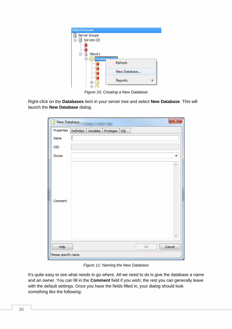
39
Figure 10: Creating a New Database
Right-click on the Databases item in your server tree and select New Database. This will
launch the New Database dialog.
Figure 11: Naming the New Database
It's quite easy to see what needs to go where. All we need to do is give the database a name
and an owner. You can fill in the Comment field if you wish; the rest you can generally leave
with the default settings. Once you have the fields filled in, your dialog should look
something like the following:

40
Figure 12: Completed New Database Dialog
Most Postgres installers create a template to aid in the creation of spatial database tables
when using this or similar dialogs. Before we click OK, we need to navigate to the Definition
tab and select the template to use as shown in the following figure:

41
Figure 13: Choosing a Template from the Definition Tab
All the other options in this tab can be left as they are. Once you click OK, pgAdmin will
return to the main display where you'll see your new database appear in the server tree.
Figure 14: New Database Added to Server Tree
It's also possible to create the database by hand using standard SQL commands such as
Create Database and Create Table; however, using these can be a lengthy process.
There are scripts in the Postgres Contrib directory (located where you chose to install
Postgres) that you can load and run to create all the spatial functions and metadata tables

42
required. Since every installation of Postgres I've done has included pgAdmin, I've found it
much easier and quicker to use the GUI. Please also note that even if you are installing your
database on a platform such as Ubuntu, the pgAdmin tool can be downloaded separately
from the Postgres website and installed on a standard Windows machine for managing your
server.
Once the database has been created, you can expand the objects in the server tree to show
the different tables and objects in your new spatial database.
Figure 15: Exploring the New Database
A Side Note about Postgres Users
Many of you reading this will likely be accustomed to using MS SQL Server for your data
tasks. Postgres, like SQL Server, supports multiple user accounts. However, you need to be
careful with using the root admin account.
In MS SQL, the super user account (usually sa) has ultimate control over the entire
database. Under Postgres, the equivalent super user account is called Postgres, but unlike
MS SQL, the Postgres user can be prevented from interacting with other tables.
If you create all your tables using the Postgres account you won't have an issue, but if you
create databases and then assign ownership of these databases to other user names you
have created in your server, you might find that the Postgres user account is unable to work
with them.
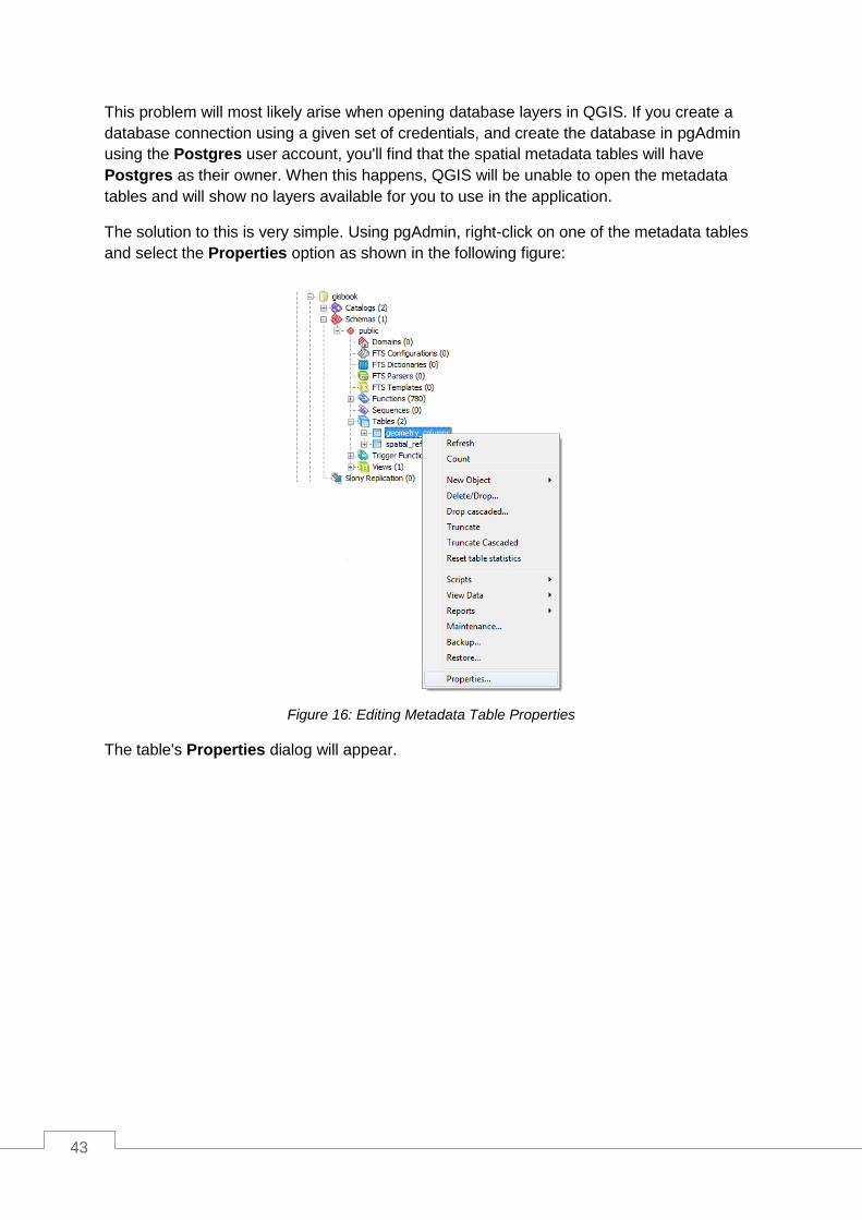
43
This problem will most likely arise when opening database layers in QGIS. If you create a
database connection using a given set of credentials, and create the database in pgAdmin
using the Postgres user account, you'll find that the spatial metadata tables will have
Postgres as their owner. When this happens, QGIS will be unable to open the metadata
tables and will show no layers available for you to use in the application.
The solution to this is very simple. Using pgAdmin, right-click on one of the metadata tables
and select the Properties option as shown in the following figure:
Figure 16: Editing Metadata Table Properties
The table's Properties dialog will appear.

44
Figure 17: Editing the geometry_columns Table Properties
The Owner field provides a drop-down list of users defined in the server. Select the owner
that you are using in your app connection.
Revisiting the Metadata Tables
If you remember from our discussion earlier in the book, we discussed the spatial metadata
tables and the importance they have in the grand scheme of things.
If you've created your spatial database correctly, you should see two tables in your server
tree: geometry_columns and spatial_sys_ref. Right-clicking on them and selecting View
Data will allow you to examine what's in them as shown in the following figures.

45
Figure 18: spatial_sys_ref Table
Figure 19: geometry_columns Table
As you can see, the geometry_columns table is initially empty. This will start to fill up as we
load data into our database.
Loading Points Using QGIS
Quantum GIS has a great little tool built-in called SPIT (Shapefile to PostGIS Import Tool)
whose sole purpose is to insert ESRI shapefiles into Postgres.

46
In practice, I have found that it gets upset easily if there's even the slightest bit of corruption
or non-standard data in the shapefile you are trying to import. Despite its fragility, it remains
the most used tool by QGIS users to import data into their database.
You activate SPIT by clicking the small blue elephant icon on your QGIS toolbar as shown in
the following picture:
Figure 20: Activating SPIT
Once SPIT loads and displays its main interface, you should see the following:
Figure 21: SPIT Interface
The interface is fairly self-explanatory. The PostgreSQL connections area is where you'll
find any connections to your SQL databases listed. The Import options are for specifying
things like the SRID of your data, and other options for the data import.
Your PostgreSQL connections list is shared between here and the main app. If you've
already created a connection in QGIS, you'll be able to reuse it here by just selecting it from
the drop-down and clicking Connect.
For the purposes of this exercise, however, we'll be creating a new connection to hold our
data. To start, click New under PostgreSQL connections. The Create a New PostGIS
connection dialog will appear.

47
Figure 22: Creating a New PostGIS Connection
Complete the fields as shown in Figure 22, remembering to substitute your server name,
database name, user name, and password as required for your own Postgres installation.
You don't have to save the password and user name, but it makes connecting easier if you
don't have to type the credentials in every time.
The four deselected options are not required. They are used to control the following:
Only look in the geometry_columns table: This option means exactly what it says.
By default, QGIS will look at all tables in the database to see if any of them contain
spatial geometry. Selecting this check box prevents this.
Only look in public schema: If you use different schemas to logically divide your
database, selecting this option will make QGIS only look in the public schema
(equivalent to DBO in MS SQL).
Also list tables with no geometry: Selecting this option will make QGIS list tables
with no geographic data in the Add Layer dialog.

48
Use estimated table metadata: If you have a table that is not registered in the
geometry_columns table, selecting this option will make QGIS guess the data type,
rather than examine the data in the table to determine the geometry type.
Once the fields are completed, click the Test Connect button. The test should be
successful.
Click OK to save the connection and register it in the SPIT tool.
Once you return to the SPIT dialog, click Connect, and then use the Add button to browse
and load the shapefiles for U.K. towns and cities.
You can download sample shapefiles from bitbucket.org/syncfusion/gis-succinctly.
Once you've set the other options such as the SRID—all files provided for these demos are
in UK-OSGB36, SRID 27700—and the Geometry column name, your SPIT dialog should
look similar to the following figure:
Figure 23: Completed SPIT Dialog
Click OK to add your data into your Postgres database and create any tables and other
objects needed. If you go back to pgAdmin after adding your data and look at the
geometry_columns table, you'll see that there are now two entries in it.
49
Once SPIT has finished, you should be able to go back to the main QGIS window and
display a Postgres vector layer. We'll wait to do this for the moment though; next we're going
to load the county boundary polygons using GeoKettle.
Loading Boundary Polygons Using GeoKettle
Sometimes you need a little bit more control over your data loading process. For instance,
you may need to combine two files and make some transformations to your data before
importing it into your database.
When you need to go beyond simple loading using SPIT, you need to use an ETL (Extract,
Transform, and Load) tool such as GeoKettle. As mentioned previously, GeoKettle is a
specialized ETL package that understands geospatial data and all its special metadata.
As with Postgres and QGIS, I'm not going to cover the installation process. It's fairly
straightforward if you download the Java installer version. Since it requires Java to run,
make sure you have an up-to-date Java VM installed on your computer.
After installing GeoKettle, open the program. You should be presented with something that
looks like the following screenshot:
Figure 24: GeoKettle Home Screen
The concepts behind using GeoKettle are slightly different than the normal point-and-click
methodology you may be familiar with, but once you get used to them working with
GeoKettle is very easy.

50
Transformations and Jobs
If you click on the File menu and select New, you'll see that you have two options:
Transformation and Job. The idea here is that many transformations make up a job,
allowing you to break your task down into smaller chunks and then reassemble them using a
sequence.
If you've ever done any workflow programming in .NET, you'll be familiar with the idea of
separate work units and sequencing those pieces to perform a whole task. Using GeoKettle
is the same idea. For what we are going to achieve here, we only need a simple
transformation, so select the Transformation item under New.
Figure 25: GeoKettle File Menu
Adding Transformation Steps
Once you have a new GeoKettle work surface, you'll notice the designer palette in the left of
your screen.
To construct a transformation, drag the necessary steps from this palette to your work
surface, and then connect them together by holding Shift and dragging between them.
Data then flows from step to step in the direction of your connections, performing the
required step as it passes through.
In order to add a shapefile to a database, we need three transformation steps:
1. A shapefile input.
2. A set SRID transform.
3. A table output.
Let's start by adding our input step. Select the Input folder in the design palette, and then
drag a Shapefile File Input onto the work surface as shown in the following screenshot:

51
Figure 26: Adding a Shapefile Input Step to the Transformation
Open the Output folder in the designer palette and add Table output to the transformation.
Figure 27: Adding a Table Output Step to the Transformation

52
Open the Transform folder in the designer palette and add the Set SRS step.
Figure 28: Adding a Set SRS Step to the Transformation
Note the black arrow in Figure 28 pointing at SRS Transformation—be careful not to use
this one as it is an actual data transformation. You may find that you need this if you're
transforming your data from one spatial system to another; for example, if you have a GPS
course recorded from a GPS device, it may be in WGS84 coordinate space, but you may
need to change it to a local UTM system that matches your area of the globe.
Set SRS does NOT transform the actual coordinate values; it simply sets the SRID of the
data you're adding. You must ensure that this SRID is the correct value; otherwise, when
you try to demonstrate or project your data, your geometry will appear in a completely
different place than where you expect it.
Once you've added the necessary steps to the workspace, you need to connect them. To do
this, click on one of your steps to select it, hold Shift, and then click and drag to the step you
wish to connect. One thing that may be confusing is that GeoKettle does not draw a line as
you drag the pointer from one step to the next. Just keep moving the pointer to your next
transformation step and release the mouse button when you reach it.
For our example, connect the Shapefile File Input to Set SRS, and then connect Set SRS
to Table output. If all goes as expected, you should see something like the following:
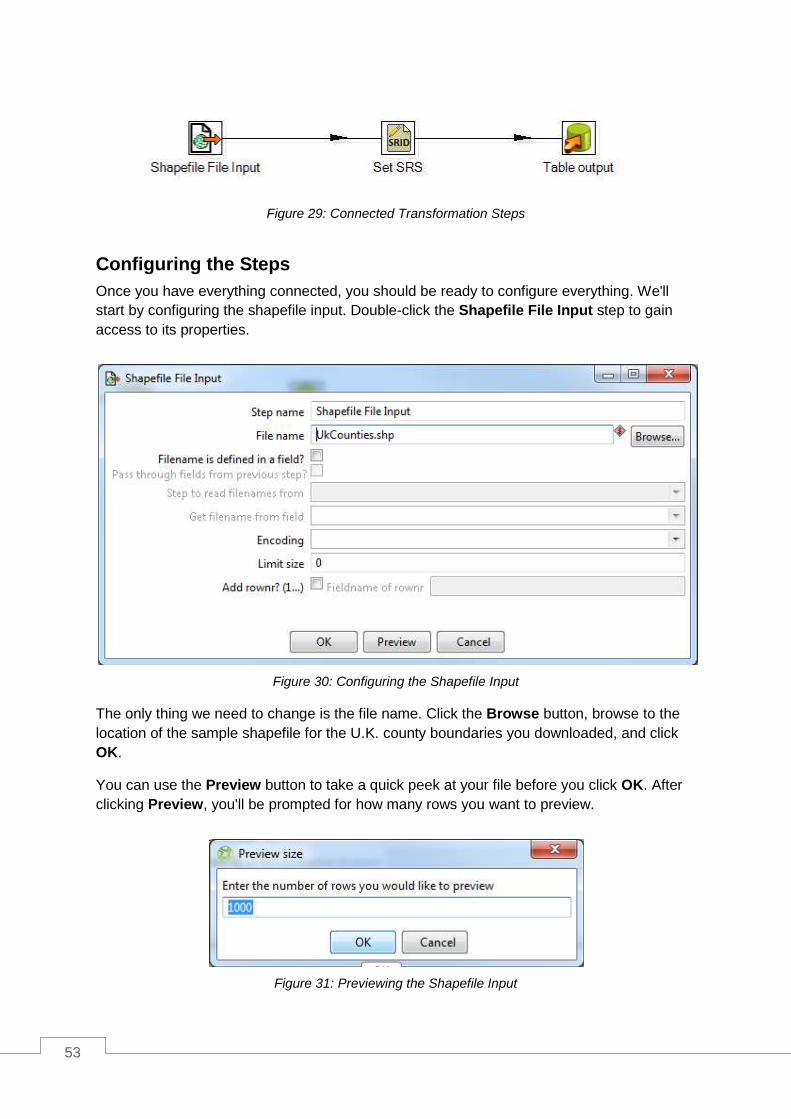
53
Figure 29: Connected Transformation Steps
Configuring the Steps
Once you have everything connected, you should be ready to configure everything. We'll
start by configuring the shapefile input. Double-click the Shapefile File Input step to gain
access to its properties.
Figure 30: Configuring the Shapefile Input
The only thing we need to change is the file name. Click the Browse button, browse to the
location of the sample shapefile for the U.K. county boundaries you downloaded, and click
OK.
You can use the Preview button to take a quick peek at your file before you click OK. After
clicking Preview, you'll be prompted for how many rows you want to preview.
Figure 31: Previewing the Shapefile Input

54
Entering 0 will show all the rows in the input file. Click OK to display the preview. GeoKettle
will open the file and show you a spreadsheet-like view of the data and any attributes within
the file.
Figure 32: Shapefile Data Preview—Standard View
You can click the Geographic view tab at the top to see the following:
Figure 33: Shapefile Data Preview—Geographic View
When you're finished previewing the data, click Close. Click OK in the Shapefile File Input
dialog to complete the shapefile input setup.
The next thing we need to do is set our SRS options. In our case, as you may have noticed
when previewing the data, our county boundaries shapefile is actually in WGS84 (SRID
4326) coordinate space. As mentioned previously, we are not going to actually transform the
coordinates for this sample data, but in a production system it's highly recommended that
you match all your data in the same coordinate space. If I was doing this for a production

55
system, I'd use the SRS Transformation step and actually change the coordinates to
OSGB36 (SRID 27700). For this example, I'm keeping things as simple as possible.
If you want to try transforming your data, note that you'll need two Set SRS steps, one on
each side of the SRS Transform step, to ensure you have the correct spatial ID going into
and coming out of the transformation.
Moving on in our example, let's set the singular SRID we need for this data. Double-click the
Set SRS step to open its dialog; you should see the following:
Figure 34: Configuring the Set SRS Step
For the Set SRS on field drop-down, select the correct field to set the geometry on. Usually
it is called the_geom in a shapefile. In the EPSG Code field, select the correct spatial ID for
the data. In our case, it will be SRID 4326 (WGS84). You can look through the drop-down list
to get an idea of how many SRID coordinate spaces there are. Rather than looking through
the entire drop-down list, you can simply type 4326.
Once you've set the SRID, click OK to confirm the SRS settings.
The final step is to set our Table output and associated database connection. Double-click
the Table output step to open its configuration dialog as shown in the figure that follows.
Note that I've already filled in the connection and target table details.

56
Figure 35: Table Output Configuration
The first thing you'll want to do is create a new database connection. Click the New button
next to the Connection field. The Database Connection dialog will appear.
Figure 36: Adding a New Database Connection

57
Again for Figure 36, I've already filled in my details, but you should easily be able to see that
GeoKettle supports a wide variety of database types.
Under Connection Type, select PostgreSQL. Under Access, select Native JDBC and fill
in the appropriate details to connect to the same database you connected to when adding
the point data using QGIS.
Once you’re done, give the connection a name and click the Test button. You should be
shown a small dialog stating that the connection to the database is OK, as shown in the
previous figure. Click OK to close the dialog, and click OK in the Database Connection
window to go back to the Table Output options.
Next, you must set a target table name so the transformation step knows where to insert the
data. You may also want to select the Truncate table check box to ensure the table is void
of data before starting. The other table output settings can usually be left as they are.
If you’re creating the data for the first time, you'll need to click the SQL button at the bottom
of the window to automatically generate and run the SQL necessary to create the initial table
in your database. If you're using an existing table, this will give you the SQL needed to
ensure the table schema matches the data. It's fairly straightforward, and if you have any
knowledge of SQL you'll see immediately what's happening.
One thing I often do in the SQL dialog is add a primary key because GeoKettle does not
automatically add one. There are transformation steps for adding primary keys and such, but
I find it easier to add the extra field in the SQL editor when creating the table by manually
typing in the extra line. In the following figure, you can see I added a primary key with the
definition for GID in Postgres.
Figure 37: Adding a Primary Key
When you're done editing your SQL, click Execute to run it. Once you've run your SQL
successfully, you can click Close to exit the SQL editor and then click OK to navigate back
to the transformation workspace. You've completed setting up the required steps.

58
When you arrive at this point, go to File > Save to save your loading script. GeoKettle will
refuse to run the transformation unless your file is saved. When your script is saved and
you're ready to run the transformation, click the green play arrow in the toolbar.
Figure 38: Button to Run Transformation
The Execute a transformation window will appear.
Figure 39: Execute a Transformation Window
99 percent of the time you won't need to change anything in this window. Click the Launch
button and the lower pane in your workspace will display the transformation progress.
Figure 40: Viewing the Transformation Results

59
When all your Active column entries switch to Finished, you should have a database
loaded with the county polygons; you are now ready to start experimenting.
If any of the steps turn red and display Stopped, you have a problem. The details and stack
trace of the problem will be shown in the Logging and Execution History tabs.
Unfortunately, as much as I'd like to be able to list every possible issue you'll see here, I
simply can't. When GeoKettle fails, it only releases a stack trace and refuses to do anything
further. This probably isn't an issue for the average developer, but for a non-technical user it
can look very scary indeed.
My experience with transformation problems is that they're usually some kind of data format
issue; for instance, an incorrect setting in the transform step of the destination server spitting
out its default data because it doesn't like something about the SQL GeoKettle has just sent
to it.
Whenever I receive a stop condition, I copy and paste the output from the Logging pane
into a text editor so I can start examining SQL statements and diagnosing the stack trace in
an easier-to-read window.
Once all of the transformation steps finish successfully, you can close GeoKettle and return
to Quantum GIS. Using the connection you created when loading data with SPIT, you can
view the data you now have in your database.
Previewing the Data
If we open Quantum GIS and start a new project, the first thing we need to do is set the
project properties. We do this by navigating to Settings > Project Properties in the toolbar.
Figure 41: Opening Project Properties in Quantum GIS

60
Figure 42: Quantum GIS Project Properties
In Project Properties, select the Enable 'on the fly' CRS transformation check box since
we have both SRID 27700 and SRID 4326 coordinate systems in our database. As you can
see in Figure 42, I've selected OSGB36 (SRID 27700) for my project since I reside in the
U.K. You can choose WGS84 for your project if you want. As mentioned previously, it's a
good practice to select a coordinate system specific to your location.
Once you've selected your coordinate system, click OK to return to the main Quantum GIS
workspace.
Now we need to start adding vector layers from our database. Click the blue Add Database
Layer icon on your toolbar. You'll be presented with the Add layers dialog, and should
immediately recognize the Connections drop-down at the top of the dialog; it looks just like
the one you used in SPIT.

61
Figure 43: Add Database Layer Icon
Figure 44: Adding Database Layers
Select the connection you wish to use from the drop-down, or create a new one as you did in
SPIT, and click Connect. A list of vector layers present in your Postgres database should
appear as shown in the following figure:

62
Figure 45: Available Vector Layers
As you can see, the two point layers we imported earlier and the polygon layer we imported
using GeoKettle are available. Select all of them and click Add.
After a bit of processing, depending on your computer and database speed, QGIS should
display the layers, hopefully in three different styles.
Figure 46: Loaded Map with Three Layers
As shown in my example in Figure 46, county boundaries are in green, towns are dark blue,
and cities are pink.
If your display looks anything like mine, then congratulations, you've just created your very
first spatially enabled database. Now we get to play with this data.

63
Chapter 4 Spatial SQL
I've mentioned this breed of SQL many times in this book, and to some extent I've also
described it in a brief fashion.
Spatial SQL is not anything special; if you take "Spatial" out of the name, it's just regular
SQL. Either way you're dealing with binary large objects, or blobs.
Just like working with images embedded in the database, these blobs have a special
meaning when processed by code that understands what they contain. It's the addition of
this code along with the extra SQL functions needed to use it that makes a spatially enabled
database.
In the following section, I'm not going to cover every possible permutation and function call.
At last count there are more than 300 independent functions in the OGC specification,
covering just about every possible scenario from spatial distance relationships, to
constructions of complex geometries, to clipping rasters for predefined vector paths.
Instead, using the data we've placed in our database, I'll guide you through some simple but
common operations—the type that anyone writing a GIS-enabled application is likely to use.
Before we discuss these operations, let's take a quick look at the input and output stages
described in the first chapter.
Creating and Retrieving Geometry
Even though we've already imported some data into our database, anyone writing a GIS app
also needs to be able to create geometry in the database, especially if the application is
going to allow editing.
Most geometry creation is performed in one of three formats:
Well-known text (WKT)
Extended well-known text (EWKT)
Well-known binary (WKB)
We'll be using WKT in the examples that follow, and we'll only be performing the operations
in SQL without inserting any data into our database. EWKT is slightly different, mostly due to
the fact that in the textual representation of the geometry, the SRID is separated from the
rest of the data by a semicolon.
I prefer to use the WKT standard and the spatial function ST_SetSrid to set the SRID for my
geometries.
If you are using MS SQL, you may have to use EWKT since it doesn't have a ST_SetSrid
function. There is, however, a writable SRID property on the Geometry SQL type.

64
So how do we create a geometry using WKT? Try the following SQL:
This creates a four-segment linestring that starts at 1,1, ends at 4,4, and passes through 2,2
and 3,3. The following is another example of creating geometry with SQL:
This creates a point at 5, 6 in the current coordinate system.
You can include an optional second parameter that specifies the SRID of the geometry. So if
we wanted to create our point in OSGB36 (SRID 27700) coordinates, we'd use the following:
If you try this using the SQL editor in pgAdmin, you'll find that the database doesn't complain
about the coordinates not being valid for the coordinate system being used. That's because
the second parameter only sets the field in the geometry blob to say what the geometry's
coordinate system is; it does not set anything in the metadata tables or anywhere else in the
system to mark that SRID.
Please also note that if you are trying to insert these geometries into a table you have
created, the triggers and constraints on those tables will have been set by the table creation
functions to allow only certain geometry types and SRIDs to be inserted. This can disrupt
many new GIS developers. If the second parameter is not specified, the database will set it
to the table default. It's all too easy to insert an invalid coordinate if you don't specify the
SRID.
If you do specify the SRID, but it doesn't match the SRID of the table you are inserting the
geometry into, then the insert will be rejected and not committed to the table. It is very
important to be sure when creating new geometries by hand that you have the correct SRID
for your data, and that it matches the constraints of any tables you may have created.
Any of the geometry types we discussed in Chapter 1 can be used in the GeomFromText
function, but beware as sometimes things are not quite as simple as you may expect,
especially when it comes to MULT geometries.
The following is a simple point type.
SELECT ST_GeomFromText('LINESTRING(1 1,2 2,3 3,4 4)')
SELECT ST_GeomFromText('POINT(5 6)')
SELECT ST_GeomFromText('POINT(5 6)',27700)
SELECT ST_GeomFromText('POINT(5 6)')

65
Multipoints, on the other hand, look like this:
As you can see, simple parenthesis nesting can quickly become a nightmare. Some of the
most bizarre bugs I've had to track down in GIS were a direct result of a missing
parenthesis.
The same format is used for all other geometry types too.
The exception to the rule is polygons. Because polygons can include inner rings, a standard
polygon actually looks like a single multipolygon from the start. This means that
multipolygons have three sets of parentheses surrounding them.
This is not very nice to debug. Using a library like DotSpatial or SharpMap helps
tremendously because it has functionality built in that allows you to use a familiar C# or VB
object and have this text, or even a direct WKB representation, generated on the fly for you
so you won't have to construct these geometries by hand.
There are other input functions besides GeomFromText. Most of them mirror the equivalent
output functions listed in the next section. For your reference, I've listed some of the input
functions available in the latest version of Postgres:
Other geometry functions available in the latest version of Postgres include:
SELECT ST_GeomFromText('POINT((5 6)(6 7))')
SELECT ST_GeomFromText('MULTILINE((1 1,2 2)(1 2,2 1))')
SELECT ST_GeomFromText('MULTILINESTRING((1 1,2 2,3 3,4 4)(5 5,6 6,7 7,8 8))')
SELECT ST_GeomFromText('POLYGON((x y,x y,x y,x y..)(x y,x y,x y,x y..))
SELECT ST_GeomFromText('MULTIPOLYGON(((x y,x y,x y,x y..) (x y,x y,x y,x y..))((x y,x y,x y,x y..) (x y,x y,x y,x y..)))')
ST_GeomFromEWKB()
ST_GeomFromEWKT()
ST_GeomFromGML()
ST_GeomFromKML()

66
All of which are detailed in the Geometry Constructors section of the online PostGIS manual
at http://postgis.refractions.net/docs/reference.html#Geometry_Constructors. Most of the
geometry constructors are also defined in the OGC specifications.
Output Functions
Now that we've seen how to generate geometry objects, it would be great to be able to get
our data back out of the database.
If you want just the binary blob representation, a simple Select will do the job. In the
creation samples in the previous section, because we weren't inserting the data, the output
was the actual binary blob that represented the geometry.
One thing you must be cautious of: when dumping the blob directly, it might not be a WKB
formatted object. Some database services store the data in an internal format which allows
them to manage it quicker and easier than if it were WKB. If you want to ensure you always
receive a WKB output, be sure to use the correct output function as shown in the following
code:
Quite a few textual output functions are available as well, such as:
This will output your geometry in the WKT format.
If you want your geometry output in the EWKT format, use the following:
If you’re displaying your geometry in an HTML 5 page using SVG, then you'll use the
following:
ST_Point()
ST_LineFromMultiPoint()
ST_Polygon()
SELECT ST_AsBinary(geometry)
SELECT ST_AsText(geometry)
SELECT ST_AsEWKT(geometry)
SELECT ST_AsSVG(geometry)

67
This returns an SVG tag ready to be inserted directly into your output or an SVG file.
If you're creating output for use in Google Earth or any other app that supports Keyhole
Markup Language, use the following function:
If you're outputting industry-standard Geography Markup Language (GML) or GeoJSON (A
special format of JSON designed especially for geographic data),
and
will be your functions.
Some servers also provide other output functions on top of that, such as the following
Postgres function:
This outputs coordinates in NMEA seconds, minutes, and degrees format, but the use of this
is considered non-standard and may make it hard to port your application between database
platforms.
Let's have a quick look at one or two of these functions using the cities point data we added
to our database. To do this, we'll use the SQL editor in pgAdmin. To open the SQL editor,
select the database you wish to work in— in our case the GISBook one if you've been
following along—and click on the SQL magnifying glass icon on the toolbar.
Figure 47: SQL Editor Icon
SELECT ST_AsKML(geometry)
SELECT ST_AsGML(geometry)
SELECT ST_AsGeoJSON(geometry)
SELECT ST_AsLatLonText(geometry)

68
This will open the SQL Editor pane.
Figure 48: SQL Editor
Type your SQL statements in the top pane, and press F5 or click the green arrow to run your
SQL. The results and messages will appear in the lower pane.
A side note on using SQL in Postgres
Using SQL in Postgres is likely to cause some users problems: Postgres is case sensitive by
default. If you create a table or other object with a name with specific casing, it will create
exactly that name. However, when trying to access the object, Postgres will look for the
object name using all lowercase letters unless the name is enclosed in quotation marks.
As an example, if I CREATE TABLE Shawty, then the table will be named Shawty with a
capital S. But if I then run SELECT * FROM Shawty, Postgres will fail to find the table.
Instead, I need to type SELECT * FROM "Shawty" to make Postgres pay attention to the
casing of the name.
This also extends to the Postgres data adapter for .NET. If you are unable to access a table
in the Postgres data adapter, try putting the table name in quotation marks and you'll most
likely find it resolves the issue.
Please note that regular strings are enclosed with single quotes, not double quotes. If you
enclose your literal string in double quotes, Postgres will interpret your text as an object
name and not as data.
The best practice for creating objects in Postgres is to give them all lowercase names. I've
done exactly this for the database I'll be using to demonstrate the SQL functions, and I've
changed all the names of tables and columns to lowercase after importing the data as shown
previously. I've also removed columns from the dataset that are unused either in the
examples, or in general.
If you receive errors while trying the samples, make sure that you're making the same
changes I am, using single and double quotes properly, and correctly casing names as
needed.

69
Testing the Output Functions
Let's try the following:
You should receive something like the following output:
Figure 49: Data Output with Binary Geometry
As you can see, the geometry column is displayed in its binary form, which may or may not
be in WKB format.
Now let's try this:
You should receive the following:
Figure 50: Data Output with Text Geometry
As shown in the previous figure, the output is in WKT format with the coordinates in meters
since we're using OSGB36 as the SRID.
Let’s swap AsText for AsEWKT. We should get the following:
SELECT * FROM ukcitys LIMIT 5
SELECT gid,number,name,admin_name,AsText(geometry) FROM ukcitys LIMIT 5

70
Figure 51: Data Output with EWKT Geometry
You may have noticed that in these examples I've been calling the functions without the ST_
in front. ST_ is a legacy tag from when systems were called Spatial and Temporal systems.
In most modern GIS databases, you can freely switch between using the prefix and leaving it
out since most systems define the function both with and without the 'ST_' prefix. One or two
functions are defined only with the ST_ prefix, so if something seems to be missing in your
data, try both spellings before you give up.
As you can see, the main difference between AsText and AsEWKT is the addition of the SRID
in the output.
Let's try one more, this time with the data output in GeoJSON format:
Figure 52: Data Output with GeoJSON Geometry
What Else Can We Do with Spatial SQL?
We can do tons of things with spatial SQL. A better question is what can't we do? However,
as a developer, you're most likely only interested in simple tasks, so we'll continue by looking
at a few real-world scenarios and what our database can do to help us.
Scenario 1: Largest land mass
Let's suppose you have a number of land plots for sale, and you have them all in a nice
mapping system that potential buyers can browse via a map-enabled website. One thing you
may want to know is which plot has the largest area so you can price them appropriately.
This is achieved very simply by using the area functions provided by the database.
SELECT gid,number,name,admin_name,ST_AsGeoJSON(geometry) FROM ukcitys LIMIT 5
SELECT name2,ST_Area(the_geom) FROM ukcountys LIMIT 5

71
Figure 53: Calculated Land Areas
You'll notice that all our results are in square degrees or fractions thereof. This is because
our geometry was added to the database in WGS84 (SRID 4326) coordinates. Most of the
calculation functions will return their answers in the same units that the source geometry
uses. Converting our area results to meters is not difficult.
SRID 27700, if you recall, is measured in meters so all we need to do is transform our
geometry from SRID 4326 to SRID 27700. We can do this using ST_Transform.
The transform function takes the geometry to be transformed as the first parameter, and the
SRID to transform it to as the second. Using the function on our data gives us the following
SQL:
Figure 54: Geometry Converted from Square Degrees to Meters
Once you have the data converted from square degrees to meters, you can then use normal
SQL order by clauses and other aggregate functions to arrange the areas from largest to
smallest, or add a price column. For example, the following code outputs the five largest
counties in the U.K. and their areas in square meters.
SELECT name2,ST_Area(ST_Transform(the_geom,27700)) FROM ukcountys LIMIT 5
SELECT name2,ST_Area(ST_Transform(the_geom,27700)) FROM ukcountys order by ST_Area(ST_Transform(the_geom,27700)) desc LIMIT 5

72
Figure 55: Five Largest Counties in the U.K in Descending Order
Another thing that might be useful to know is how long the perimeter of the land mass is.
Finding this is just as easy, as shown in the following code sample and data output:
Figure 56: Perimeter of U.K. Counties
Scenario 2: How many of what are where?
Another typical use of GIS is for gathering information on how one object's location is related
to another object's location. For example, given three U.K. counties—Durham, Tyne and
Wear, and Cumbria—we can easily find out how many principal towns are in each.
This code gives us the following:
SELECT name2,ST_Perimeter(ST_Transform(the_geom,27700)) FROM ukcountys LIMIT 5
SELECT ukcountys.name2,count(uktowns.*)
FROM ukcountys,uktowns
WHERE ST_Within(uktowns.geometry,ST_Transform(ukcountys.the_geom,27700)) AND ukcountys.name2 IN ('Durham','Tyne and Wear','Cumbria')
GROUP BY ukcountys.name2
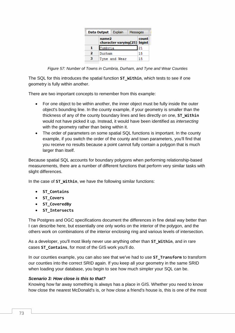
73
Figure 57: Number of Towns in Cumbria, Durham, and Tyne and Wear Counties
The SQL for this introduces the spatial function ST_Within, which tests to see if one
geometry is fully within another.
There are two important concepts to remember from this example:
For one object to be within another, the inner object must be fully inside the outer
object's bounding line. In the county example, if your geometry is smaller than the
thickness of any of the county boundary lines and lies directly on one, ST_Within
would not have picked it up. Instead, it would have been identified as intersecting
with the geometry rather than being within it.
The order of parameters on some spatial SQL functions is important. In the county
example, if you switch the order of the county and town parameters, you'll find that
you receive no results because a point cannot fully contain a polygon that is much
larger than itself.
Because spatial SQL accounts for boundary polygons when performing relationship-based
measurements, there are a number of different functions that perform very similar tasks with
slight differences.
In the case of ST_Within, we have the following similar functions:
ST_Contains
ST_Covers
ST_CoveredBy
ST_Intersects
The Postgres and OGC specifications document the differences in fine detail way better than
I can describe here, but essentially one only works on the interior of the polygon, and the
others work on combinations of the interior enclosing ring and various levels of intersection.
As a developer, you'll most likely never use anything other than ST_Within, and in rare
cases ST_Contains, for most of the GIS work you'll do.
In our counties example, you can also see that we've had to use ST_Transform to transform
our counties into the correct SRID again. If you keep all your geometry in the same SRID
when loading your database, you begin to see how much simpler your SQL can be.
Scenario 3: How close is this to that?
Knowing how far away something is always has a place in GIS. Whether you need to know
how close the nearest McDonald's is, or how close a friend's house is, this is one of the most
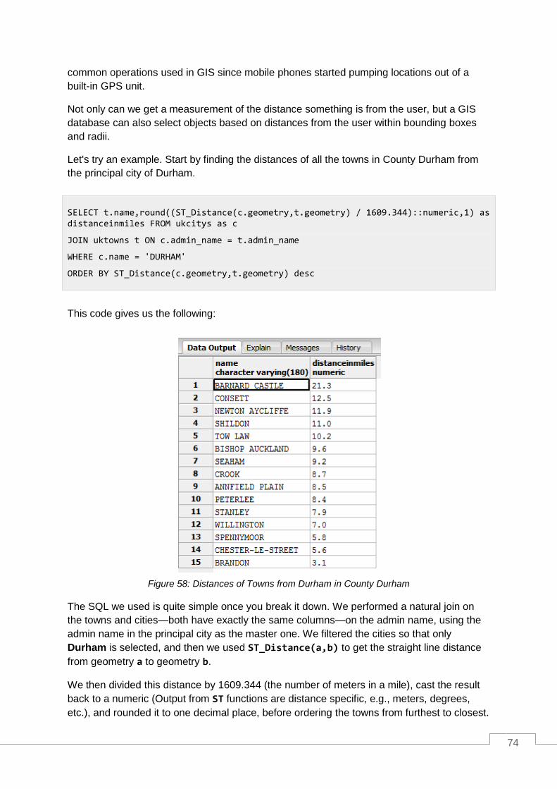
74
common operations used in GIS since mobile phones started pumping locations out of a
built-in GPS unit.
Not only can we get a measurement of the distance something is from the user, but a GIS
database can also select objects based on distances from the user within bounding boxes
and radii.
Let's try an example. Start by finding the distances of all the towns in County Durham from
the principal city of Durham.
This code gives us the following:
Figure 58: Distances of Towns from Durham in County Durham
The SQL we used is quite simple once you break it down. We performed a natural join on
the towns and cities—both have exactly the same columns—on the admin name, using the
admin name in the principal city as the master one. We filtered the cities so that only
Durham is selected, and then we used ST_Distance(a,b) to get the straight line distance
from geometry a to geometry b.
We then divided this distance by 1609.344 (the number of meters in a mile), cast the result
back to a numeric (Output from ST functions are distance specific, e.g., meters, degrees,
etc.), and rounded it to one decimal place, before ordering the towns from furthest to closest.
SELECT t.name,round((ST_Distance(c.geometry,t.geometry) / 1609.344)::numeric,1) as distanceinmiles FROM ukcitys as c
JOIN uktowns t ON c.admin_name = t.admin_name
WHERE c.name = 'DURHAM'
ORDER BY ST_Distance(c.geometry,t.geometry) desc
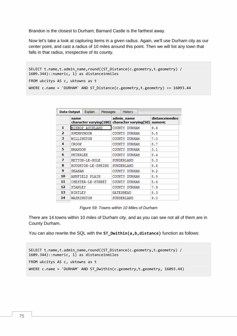
75
Brandon is the closest to Durham; Barnard Castle is the farthest away.
Now let's take a look at capturing items in a given radius. Again, we'll use Durham city as our
center point, and cast a radius of 10 miles around this point. Then we will list any town that
falls in that radius, irrespective of its county.
Figure 59: Towns within 10 Miles of Durham
There are 14 towns within 10 miles of Durham city, and as you can see not all of them are in
County Durham.
You can also rewrite the SQL with the ST_Dwithin(a,b,distance) function as follows:
SELECT t.name,t.admin_name,round((ST_Distance(c.geometry,t.geometry) / 1609.344)::numeric, 1) as distanceinmiles
FROM ukcitys AS c, uktowns as t
WHERE c.name = 'DURHAM' AND ST_Distance(c.geometry,t.geometry) <= 16093.44
SELECT t.name,t.admin_name,round((ST_Distance(c.geometry,t.geometry) / 1609.344)::numeric, 1) as distanceinmiles
FROM ukcitys AS c, uktowns as t
WHERE c.name = 'DURHAM' AND ST_Dwithin(c.geometry,t.geometry, 16093.44)

76
The only thing different is the <= clause in the last part of the WHERE statement, so what
changes? Not much, really. However, if you're using bounding boxes and buffers, you'll often
get better results using ST_Distance with a <= operator.
Again, we used the cast operator to make sure our data output a normal numeric type and
rounded it to one decimal place, divided it by 1609.344 to convert it to miles, and finally
filtered things so that only towns around Durham were included.
It's easy enough to exchange the Durham city geometry for a GPS point from a GPS device,
for example, and list the towns around that point.
Or if your GPS is WGS84 (SRID 4326), you'll need to transform it to meters and OSGB36
(SRID 27700).
Scenario 4: What is my geometry made of?
In some cases you may need to take your geometry apart and reassemble it in a different
way, or make a new geometry based on the original one.
First off, let's find out how many points make up the border around County Durham.
Figure 60: Number of Border Points
SELECT t.name,t.admin_name,round((ST_Distance(ST_Point(428110 542709),t.geometry) / 1609.344)::numeric, 1) as distanceinmiles
FROM ukcitys AS c, uktowns as t
WHERE c.name = 'DURHAM' AND ST_Dwithin(ST_Point(428110 542709),t.geometry, 16093.44)
SELECT t.name,t.admin_name,round((ST_Distance(ST_Transform(ST_Point(-1.56450 54.77851),27700),t.geometry) / 1609.344)::numeric, 1) as distanceinmiles
FROM ukcitys AS c, uktowns as t
WHERE c.name = 'DURHAM' AND ST_Dwithin(ST_Transform(ST_Point(-1.56450 54.77851),27700),t.geometry, 16093.44)
SELECT name2,ST_NPoints(the_geom) FROM ukcountys WHERE name2 = 'Durham'
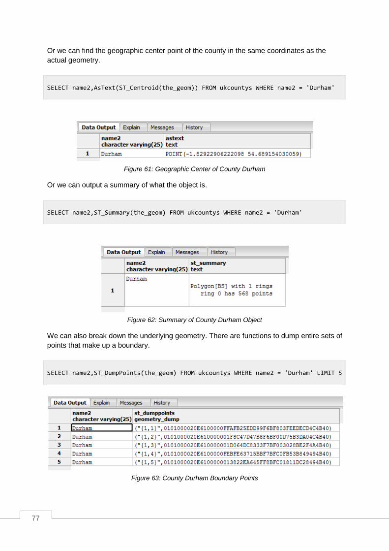
77
Or we can find the geographic center point of the county in the same coordinates as the
actual geometry.
Figure 61: Geographic Center of County Durham
Or we can output a summary of what the object is.
Figure 62: Summary of County Durham Object
We can also break down the underlying geometry. There are functions to dump entire sets of
points that make up a boundary.
Figure 63: County Durham Boundary Points
SELECT name2,AsText(ST_Centroid(the_geom)) FROM ukcountys WHERE name2 = 'Durham'
SELECT name2,ST_Summary(the_geom) FROM ukcountys WHERE name2 = 'Durham'
SELECT name2,ST_DumpPoints(the_geom) FROM ukcountys WHERE name2 = 'Durham' LIMIT 5

78
Or we can get a specific point if the input is a LINESTRING or MULTILINESTRING.
Figure 64: Finding a Specific Point
The point output shown in the previous figure is the second point in our linestring.
If you need to know the bounding box of an object, you can easily get the x, y pairs of the
maximum and minimum extents by using the following code:
Figure 65: Maximum and Minimum Extents
Or if we need to perform measurements and other functions on our extents, we can get them
as an actual geometric rectangle.
Figure 66: Extents Output as Geometric Rectangle
Lastly, let's imagine we have a segment of a path, represented by the following line:
SELECT AsText(ST_PointN(GeomFromText('LINESTRING(1 1,2 2,3 3,4 4)'),2))
SELECT name2,ST_Xmax(the_geom),ST_Ymax(the_geom),ST_Xmin(the_geom),ST_Ymin(the_geom) FROM ukcountys WHERE name2 = 'Durham'
SELECT name2,AsText(GeomFromText(box2d(the_geom)::geometry)) FROM ukcountys WHERE name2 = 'Durham'
LINE(1 1,10 10)
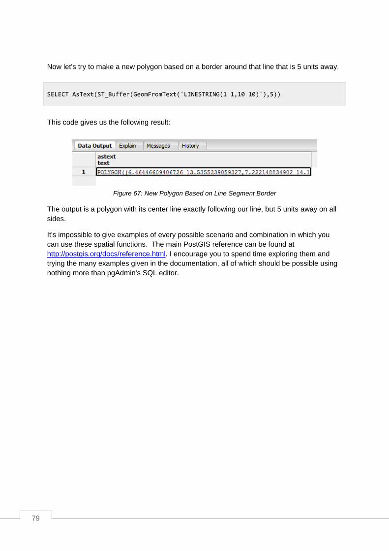
79
Now let's try to make a new polygon based on a border around that line that is 5 units away.
This code gives us the following result:
Figure 67: New Polygon Based on Line Segment Border
The output is a polygon with its center line exactly following our line, but 5 units away on all
sides.
It's impossible to give examples of every possible scenario and combination in which you
can use these spatial functions. The main PostGIS reference can be found at
http://postgis.org/docs/reference.html. I encourage you to spend time exploring them and
trying the many examples given in the documentation, all of which should be possible using
nothing more than pgAdmin's SQL editor.
SELECT AsText(ST_Buffer(GeomFromText('LINESTRING(1 1,10 10)'),5))
80
Chapter 5 Creating a GIS application in .NET
So finally we come to the part most of you have been waiting for: the creation of a small GIS-
enabled desktop application in .NET.
In this chapter I use Visual Studio 2010 Ultimate for any screenshots, and my code is in C#.
For anyone who has used any of the Microsoft .NET languages and editors, it shouldn't be
much of a problem for you to adapt what I show here to the environment you are working in.
Downloading SharpMap
Before we do anything, we need to download SharpMap; it is the GIS framework we'll be
using. Since SharpMap is currently undergoing a lot of changes and general refactoring, it's
better to download the source files from SVN and compile your own version than it is to use
the pre-compiled downloads.
In your browser, navigate to http://sharpmap.codeplex.com/ and click the Source Code tab.
Click Download to get the latest changeset as a zip file—it's approximately 180 MB. Or you
can click Connect to get the addresses to connect to either the TFS or SVN repositories
using regular clients.
Once you have the sources synced or unpacked onto your hard drive, start Visual Studio,
open the trunk folder, and open the SharpMap.sln solution.
Once everything is loaded, the Solution Explorer should appear as it does in the following
screenshot:

81
Figure 68: SharpMap Solution
If everything loaded OK, you should be able to click Build Solution to get the current
binaries. I generally build all the configurations, so I select Release then Build, Debug then
Build, and so on. What you choose to build is up to you though.
Once everything builds successfully, you're ready to close this project and start on your own.
Creating Our Own SharpMap Solution
Run an instance of Visual Studio or reuse the one you still have open, and create a new
Windows Forms app.

82
Figure 69: Starting a New Windows Forms App
Make sure you’re using .NET 4. The current version of SharpMap is targeted at .NET 4 and
above.
The first thing you need to do is double-click on Properties in the Solution Explorer and
change the selected Target framework from .NET Framework 4 Client Profile to the full
.NET Framework 4.
Figure 70: Changing the Target Framework
Now we need to add the SharpMap UI components to our toolbox. Double-click Form1.cs in
the Solution Explorer to load the toolbar palettes. Right-click in an open area below
General and select Add Tab. Give the tab a name. In my application, I called the tab
SharpMap.
Once the palette is created, expand it and right-click the Palette area. Select Choose Items
from the menu that appears. The Choose Toolbox Items dialog should appear.

83
Figure 71: Choosing Toolbox Items
Click the Browse button and navigate to the location where you unpacked the SharpMap
toolkit. Navigate to SharpMap.UI > bin > Debug, and then select SharpMap.UI.dll.
Figure 72: Adding SharpMap to the Toolbox
Click Open and then navigate back to the main Visual Studio screen. You should be greeted
with the following in your toolbox:

84
Figure 73: SharpMap and Tools in the Toolbox
You may also find that SharpMap and SharpMap.UI have been automatically added to your
project references. If you started a new project and already had the tools loaded into your
toolbox, then you'll need to add the references to your project manually. To do this, right-
click References in your project, and then browse to the same location where you added the
SharpMap.UI.dll. Add the SharpMap.dll and SharpMap.UI references. After adding these
DLLs, reload the References dialog.
We need to add some more DLLs which are located in other folders in the solution.
Browse to the SharpMap.Extensions project folder, and into Bin > Debug or Release as
needed. Select and add the following DLLs:
BruTile.dll
GeoAPI.dll
Npgsql.dll
SharpMap.Extensions.dll
Your project references should look something like the following screenshot:

85
Figure 74: Added References
Now we are ready to put our GUI together.
Set the size of your form to around 1000 x 800, change the StartPosition property to
CenterScreen, and change the title text to Sharp Map Example 1.
I generally rename my forms to something like formMainForm, but it's entirely up to you
what name to choose. If you name your forms something different, you'll need to adjust the
source accordingly when we start coding.
Now we need to drag five components onto our form in the designer. They are:
MapBox from the SharpMap tools.
Two Button controls and a ListBox from Common Controls.
StatusStrip from Menus and Toolbars.
Rename the two buttons to btnZoomAndPan and btnQueryCounty. Change the display
text on them to Switch to Zoom & Pan Mode and Switch to County Query Mode,
respectively, and then place them in the upper left corner of your form. Resize them as
needed to fit the text.
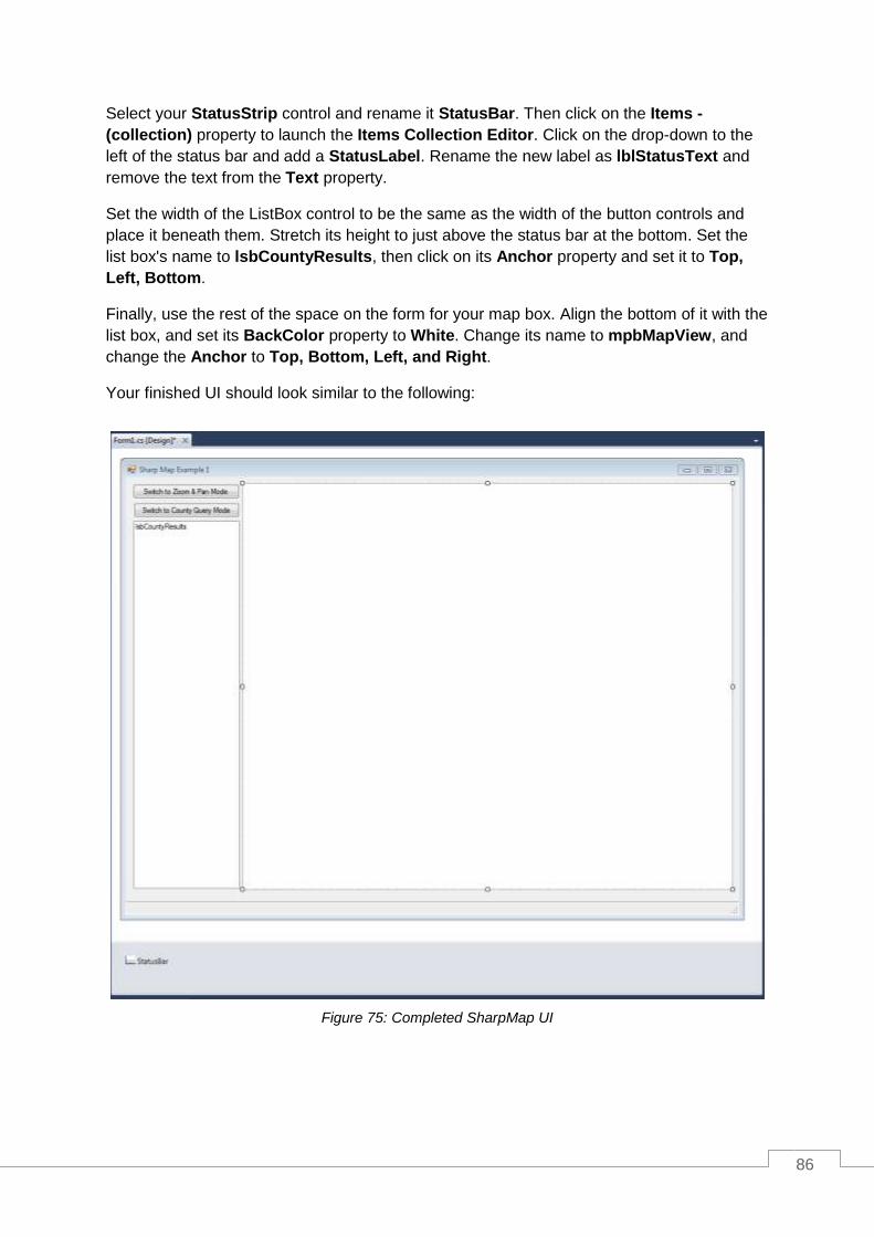
86
Select your StatusStrip control and rename it StatusBar. Then click on the Items -
(collection) property to launch the Items Collection Editor. Click on the drop-down to the
left of the status bar and add a StatusLabel. Rename the new label as lblStatusText and
remove the text from the Text property.
Set the width of the ListBox control to be the same as the width of the button controls and
place it beneath them. Stretch its height to just above the status bar at the bottom. Set the
list box's name to lsbCountyResults, then click on its Anchor property and set it to Top,
Left, Bottom.
Finally, use the rest of the space on the form for your map box. Align the bottom of it with the
list box, and set its BackColor property to White. Change its name to mpbMapView, and
change the Anchor to Top, Bottom, Left, and Right.
Your finished UI should look similar to the following:
Figure 75: Completed SharpMap UI

87
Adding the Code
Now that we have a good-looking UI, it's time to start adding functionality to our app.
Using the MapBox control is very easy. The concept is simply to create layers, and then add
those layers to the control which will then render and display them.
Each layer can have a different spatial reference and coordinate system, and the map
control can re-project and convert coordinates on the fly. For this example though, we're
going to let Postgres do all the work for us.
Load and run pgAdmin, and log into your database containing the data we loaded earlier.
Expand the object tree until you can see all your tables and other objects.
Figure 76: Object Tree in pgAdmin
As you can see in the figure, beneath the Tables node is a small green icon named Views.
You may have used these before in other databases. The general idea is that they project
data from other tables into a different schema, but appear to client apps as though they were
an actual table.
A typical use is to take rows from different tables linked via foreign keys, and present a
simple flat view of the combined data in which all the present items form a single row rather
than a hierarchy.
For our demo, we are going to re-project our town and city points as WGS84 (SRID 4326) to
match the coordinates of the U.K. counties layer. We'll start by right-clicking on Views and
creating a new view.

88
Figure 77: Creating a New View
Give the view a name—I named mine ukcitys_wgs—and set the correct user for your
database login.
Switch to the Definition tab and enter the following SQL:
Figure 78: Setting the Database Login
SELECT ukcitys.gid, ukcitys.number, ukcitys.name, ukcitys.admin_name, st_transform(ukcitys.geometry, 4326) AS geometry FROM ukcitys;

89
As you can see in our SQL and Figure 78, we are using ST_Transform to transform our
points from OSGB36 (SRID 27700) to WGS84 (SRID 4326). The result is that when a
SELECT from ukcitys_wgs is performed, the table layout will be identical to ukcitys, but the
geometry will be in the new coordinate system.
Views solve lots of problems like this in a GIS, and you'll tend to find that GIS databases
make very extensive use of them.
Repeat these steps and create uktowns_wgs using the following SQL:
One Small Problem...
For all that views do, they do have one small problem when it comes to using them in this
way: the spatial metadata.
If you recall the beginning of the book, we discussed the geometry_columns table and its
importance in the GIS database. When we create tables in the regular table space, we
generally use the spatial function AddGeometryColumn to add the column that will contain
the actual geometry object. You should have seen this happen when you used GeoKettle to
add the county data—the SQL that was generated to create the table should have contained
the AddGeometryColumn spatial function. This not only adds the column and modifies the
table as needed, but it also registers the field with the required metadata tables and sets up
some triggers to enforce the correct data types and SRIDs.
The problem is because a view is built from existing columns, there is no way of creating an
actual geometric column on a view. This means that we have to add it manually. Fortunately,
it's not a particularly difficult process; it only involves an insert.
Open up an SQL editor window and enter the following SQL:
If you examine the rows already in geometry_columns, you'll notice that the data being
inserted is identical to the row for uktowns; the only difference is the SRID.
To complete this task, perform the following to update for the city view:
SELECT uktowns.gid, uktowns.number, uktowns.name, uktowns.admin_name, st_transform(uktowns.geometry, 4326) AS geometry FROM uktowns;
INSERT INTO geometry_columns(f_table_catalog,f_table_schema,f_table_name,f_geometry_column,coord_dimension,srid,type) VALUES('','public','uktowns_wgs','geometry',2,4326,'MULTIPOINT')

90
Once you are done, you should have the following:
Figure 79: Adding New Views
INSERT INTO geometry_columns(f_table_catalog,f_table_schema,f_table_name,f_geometry_column,coord_dimension,srid,type) VALUES('','public','ukcitys_wgs','geometry',2,4326,'MULTIPOINT')

91
Figure 80: Table with New Views
SharpMap, like any decent implementation of an OGC-compliant GIS database client, will
examine the geometry_columns table to find out the details of any layers we add. It will
cancel and produce an exception if we add a view that can't be found in the
geometry_columns table. Once we manually add the data, we can then load those views into
our application.
Back to the Code...
Now that we have our UI, our data, and some views to project our data, it's time to add some
C# to stitch it all together.
The first thing we need is a connection string for our Postgres database and a Boolean flag
for the map initialization. Add the following code just before the constructor for your first
form, and substitute the sever name, passwords, and user names as needed for your own
connection:
Note that I set the command timeout to five minutes. If you're going to be doing a lot of
server-based, long running geometry processing jobs, then this is a wise thing to do. The
default command timeout is 20 seconds. When you start doing bigger jobs with this stuff,
you'll end up with gigabytes of data and some lengthy run times.
private const string _connString = "Server=<server>;Port=5432;User Id=<user>;Password=<password>;Database=gisbook;CommandTimeout=300";
private bool _mapInitializing;

92
Following our constructor, we need a function for initializing our map to be called from it.
Your code should look like this by now:
Initializing the map
The first thing we need to do in our map initialization function is set up and load our layers.
We'll start with the county layer. The data source for the vector layer requires the names of
the geometry column and the primary key—otherwise known as OID or GID in geospatial
terms—which you must have in your geometry table, and the name of the table containing
your layer.
The code to initialize and load the county layer, give it a green fill, and set a black border
style is as follows:
using System.Windows.Forms;
namespace SharpMapExample1
{
public partial class formMainForm : Form
{
private const string _connString = "Server ;Port=5432;User Id= ;Password= ;Database=gisbook;CommandTimeout=300";
private bool _mapInitializing;
public formMainForm()
{
InitializeComponent();
}
public void InitializeMap()
{
}
}
}
const string countyTableName = "ukcountys";
const string countyGeometryColumnName = "the_geom";

93
We repeat this pattern two more times to load the data for our towns and cities:
const string countyGidColumnName = "gid";
VectorStyle ukCountyStyle = new VectorStyle { Fill = Brushes.Green, Outline =
Pens.Black, EnableOutline = true };
VectorLayer ukCountys = new VectorLayer("ukcountys")
{
Style = ukCountyStyle,
DataSource = new PostGIS(_connString, countyTableName,
countyGeometryColumnName,countyGidColumnName),
MaxVisible = 40000
};
const string cityTableName = "ukcitys_wgs";
const string cityGeometryColumnName = "geometry";
const string cityGidColumnName = "gid";
const string townTableName = "uktowns_wgs";
const string townGeometryColumnName = "geometry";
const string townGidColumnName = "gid";
VectorStyle ukCountyStyle = new VectorStyle { Fill = Brushes.Green, Outline =
Pens.Black, EnableOutline = true };
VectorStyle ukCityStyle = new VectorStyle { PointColor = Brushes.OrangeRed };
VectorLayer ukCitys = new VectorLayer("ukcitys")
{
Style = ukCityStyle,
DataSource = new PostGIS(_connString, cityTableName, cityGeometryColumnName,
cityGidColumnName),
MaxVisible = 40000
};
VectorStyle ukTownStyle = new VectorStyle { PointColor = Brushes.DodgerBlue };
VectorLayer ukTowns = new VectorLayer("uktowns")
{
Style = ukTownStyle,

94
The only difference here is that we set the point color rather than the fill and line colors as
we do for a polygon layer. We set the Style property of the layers to our VectorStyle
object to give the layers their visual appearance. Next, we set the DataSource property to a
connection to our Postgres server using the constants and connection string we previously
defined. MaxVisible is the maximum zoom level that objects will be visible at in our map
viewer. If we zoom beyond the value we specify, nothing will be drawn on the screen.
After we define the layers and their styles and connections, we then simply add these layers
to the map control on our form.
Then we set our default tool, zoom to the full extents of the map, and render it.
We'll finish by inserting the following code as the first two lines of the function; this will add a
status message to our status bar while the map is initializing:
Your code should now look something like the following image:
DataSource = new PostGIS(_connString, townTableName, townGeometryColumnName,
townGidColumnName),
MaxVisible = 40000
};
mpbMapView.Map.Layers.Add(ukCountys);
mpbMapView.Map.Layers.Add(ukCitys);
mpbMapView.Map.Layers.Add(ukTowns);
mpbMapView.ActiveTool = MapBox.Tools.Pan;
mpbMapView.Map.ZoomToExtents();
mpbMapView.Refresh();
_mapInitializing = true;
lblStatusText.Text = "MAP Initializing please wait";

95
Figure 81: Nearly Completed Code
Lastly, add a call to InitializeMap() to your form constructor just below the call to
InitializeComponent(), and that's all that's needed for the initialization function.
If you run your app at this point, and everything has been set up correctly, you should see
your map layers appear on screen. You should be able to pan them by dragging the pointer
around the map surface, and zoom using the mouse wheel.
It should look something like this:

96
Figure 82: Completed Map
Fixing the Status Label
You'll notice that the MAP Initializing message in the status bar never changes. We'll fix
that. When the map finishes rendering, it fires an event called MapRefreshed.
Figure 83: Map Events

97
We hook this event in our code and add some code to it to change the label. However, we
also need to use our Boolean variable to control it as we don't want it called every time our
map is refreshed (which will happen quite often).
Hook the event with the following code:
If you run it now, the status bar should update when the map has finished rendering.
Wiring up the Tool Buttons
Now we'll add the code for the two buttons that allow you to switch tools.
SharpMap has a number of different tool modes, from zooming and panning to drawing lines
and polygons over the top of your loaded map.
The two tools we'll use in this app are the zoom and pan tool, which is the default, and the
query tool.
Changing the tool is as simple as assigning a new value to the ActiveTool property of the
MapBox control on your form. The value to assign is any of the values from the
MapBox.Tools type enumeration.
Double-click on each button in turn and add the following code in each of their click handlers
as follows:
private void MapBox1MapRefreshed(object sender, EventArgs e)
{
if(_mapInitializing)
{
_mapInitializing = false;
lblStatusText.Text = "MAP Initialized";
}
}
private void BtnZoomAndPanClick(object sender, System.EventArgs e)
{
mpbMapView.ActiveTool = MapBox.Tools.Pan;
}
private void BtnQueryCountyClick(object sender, System.EventArgs e)

98
If you run the app now, you should be able to change modes using the two buttons in the top
left of the form. Zooming and panning are handled automatically. For queries, we have to
respond to the click event on the map box and add some code to get the results we need.
Adding Our County Info Query Code
The first thing we need to do is make sure we are using the Query tool and go no further if
we are not.
From the designer, find the Click event on the map control and add the following line to the
event handler in the code:
Why do it this way? That's a very good question, especially considering that the query tool
actually has its own event handler that is fired when the map is clicked.
While writing this book, I originally used the dedicated handler, but found it quite difficult to
narrow down its range and the items I was selecting. Instead of one polygon, I routinely
received what seemed like half of the database, and had a difficult time sifting through the
amount of data handed to the event handler.
After a bit of research, it appears that most of the examples and recommended ways of
avoiding this problem involve trapping either the MouseUp and MouseDown events, or the
Click event. I chose the Click event for simplicity.
Once we know that we're in the correct tool, we can see where we are on the map. The first
thing we must do is get the actual mouse position in pixels. Then, we use ImageToWorld
from the SharpMap toolkit to transform the mouse position's x and y values into a WGS84
latitude and longitude.
Next, we need to use that position to query our county layer and gather a FeatureDataSet
containing any polygons that are present in the location we clicked.
{
mpbMapView.ActiveTool = MapBox.Tools.Query;
}
if (mapBox1.ActiveTool != MapBox.Tools.Query) return;
FeatureDataSet selectedGeometry = new FeatureDataSet();
VectorLayer theLayer =
(VectorLayer)mapBox1.Map.FindLayer("ukcountys").FirstOrDefault();
if (theLayer != null)

99
This should result in our FeatureDataSet collection being filled with any geometry found at
that location, which in our case should be the county that we clicked on.
Next up, we need to check if we have any data in the FeatureDataSet. If we do, grab the
name of the county that was clicked on.
Each row in the FeatureDataSet is pretty much the same as a row in a normal data set, so
we can look for a column with the same name as a column in the underlying table in
Postgres. If no rows are found, it's better to return.
Once we have a county name from our U.K. counties layer, we then want to get a list of
cities and towns for our county. We do this with the following two methods:
Now that we have our data, we want to provide some visual feedback to the user. First, we'll
highlight the county we clicked on.
{
if (!theLayer.DataSource.IsOpen)
{
theLayer.DataSource.Open();
}
Envelope boundingBox = new Envelope(wgs84Location.CoordinateValue);
if (Math.Abs(boundingBox.Area - 0.0) < 0.01)
{
boundingBox.ExpandBy(0.01);
}
theLayer.DataSource.ExecuteIntersectionQuery(boundingBox, selectedGeometry);
theLayer.DataSource.Close();
}
if (selectedGeometry.Tables[0].Count <= 0) return;
string countyName = selectedGeometry.Tables[0].Rows[0]["name2"].ToString();
List<string> cityList = GetCitysForCounty(countyName);
List<string> townList = GetTownsForCounty(countyName);

100
We do this by first checking to see if we already have a highlight layer on our map. If one is
not present, create a new one. One thing to note about setting the style on the highlight layer
is the way we set the color. We use the full ARGB color call so that we can specify a
transparency level to our layer—the first value in the function, 64—that allows us to see the
existing map elements underneath it.
Next we take the FeatureDataSet we obtained earlier and assign it as the data source for
our highlight layer so that the selected county polygon shows up with our defined semi-
transparent style. Note that this will highlight multiple polygons if you select more than one
on the map. Previously selected counties will be cleared.
Once we add the highlight layer and refresh the map, our selected county should be visible.
The last thing to do for our country query feature is add our county info to the list box on the
left of our UI, and add some code at the start and end of the method to show what's
happening in our status bar.
VectorLayer highlightLayer = (VectorLayer)
mpbMapView.Map.FindLayer("highlight").FirstOrDefault();
if (highlightLayer == null)
{
Color myColor = Color.FromArgb(64,144,238,144);
Brush fillBrush = new SolidBrush(myColor);
highlightLayer = new VectorLayer("highlight");
VectorStyle highlightStyle = new VectorStyle
{Fill = fillBrush, Outline = Pens.White, EnableOutline = true};
highlightLayer.Style = highlightStyle;
}
highlightLayer.DataSource = new GeometryProvider(selectedGeometry.Tables[0]);
mpbMapView.Map.Layers.Add(highlightLayer);
mpbMapView.Refresh();
lsbCountyResults.Items.Clear();
lsbCountyResults.Items.Add("Selected county: " + countyName.ToUpper());
lsbCountyResults.Items.Add("");

101
Next, we add the status bar message just after the first if statement.
And we add the completed message just before the closing brace.
Before we go any further, some of you will say, "Wow, what a long method," and wonder
why I'm using Application.DoEvents to make sure the label is updated in an event
handler. Please remember that this is example code only; it's not supposed to be a perfect
example, or simply copy and pasted verbatim to make production-quality apps. Its purpose is
purely to show you how to use SharpMap to create a simple GIS application.
if (cityList.Count > 0)
{
lsbCountyResults.Items.Add("Citys in this county");
foreach (string city in cityList)
{
lsbCountyResults.Items.Add(city);
}
lsbCountyResults.Items.Add("");
}
if (townList.Count > 0)
{
lsbCountyResults.Items.Add("Towns in this county");
foreach (string town in townList)
{
lsbCountyResults.Items.Add(town);
}
lsbCountyResults.Items.Add("");
}
lblStatusText.Text = "Querying Map... please wait for results.";
Application.DoEvents();
lblStatusText.Text = "Query finished.";

102
Conclusion
The final thing we need to do is create the two methods to retrieve our city and town lists
from our GIS database.
SharpMap is perfectly capable of taking the polygon outline we found earlier and querying
the other layers in the map to tell us which points fall within which area. However, as this
book is primarily about using a GIS database, I'd like to conclude by letting Postgres do the
heavy lifting for us once more.
The two methods are fairly similar, so I've copied both of them out and just described them
as one.
private static List<string> GetTownsForCounty(string countyName)
{
string sql =
string.Format(
"SELECT t.Name FROM ukcountys c, uktowns t WHERE name2 = :county AND
ST_Within(t.geometry,ST_Transform(c.the_geom,27700))");
List<string> results = new List<string>();
using (NpgsqlConnection conn = new NpgsqlConnection(_connString))
{
conn.Open();
using (NpgsqlCommand command = new NpgsqlCommand(sql, conn))
{
command.Parameters.Add(new NpgsqlParameter("county", NpgsqlDbType.Varchar));
command.Parameters[0].Value = countyName;
using (NpgsqlDataReader dr = command.ExecuteReader())
{
while (dr.Read())
{
results.Add(dr.GetString(0));
}
}
}
}
return results;

103
Anyone who has done any raw ADO.NET programming should immediately recognize what
we are doing here, and may even quite reasonably ask why we're not using LINQ to SQL, or
Entity Framework, or…the list goes on.
In the first place, the raw Postgres data provider doesn't provide an Entity Framework or
LINQ-to-SQL data model provider. Secondly, since we're using spatial functions, it's far
better to do this in ADO.NET than in a model where the SQL-level syntax is deeply hidden
from view.
}
private static List<string> GetCitysForCounty(string countyName)
{
string sql =
string.Format(
"SELECT t.Name FROM ukcountys c, ukcitys t WHERE name2 = :county AND
ST_Within(t.geometry,ST_Transform(c.the_geom,27700))");
List<string> results = new List<string>();
using (NpgsqlConnection conn = new NpgsqlConnection(_connString))
{
conn.Open();
using (NpgsqlCommand command = new NpgsqlCommand(sql, conn))
{
command.Parameters.Add(new NpgsqlParameter("county", NpgsqlDbType.Varchar));
command.Parameters[0].Value = countyName;
using (NpgsqlDataReader dr = command.ExecuteReader())
{
while (dr.Read())
{
results.Add(dr.GetString(0));
}
}
}
}
return results;
}

104
The first thing we do is make a constant string of the SQL we wish to run in the database,
and I'd like you to pay particular attention to :county in the query string. This is one of the
places where the Postgres data provider differs from the regular ADO.NET way of providing
parameters to a query string.
In regular ADO.NET code, parameters are usually prefixed with @, e.g., @county. In
Postgres, parameters are prefixed with a :. In code, however, adding parameters is done in
the same way.
The rest is fairly self-explanatory. We open a connection using the connection string we
defined previously, open the database, add the parameter, and run our SQL before finally
getting a data reader object to read our results into a generic string list.
We're doing all of this in nested using statements, which means everything is IDisposable
and should be freed correctly once we're done, leaving us to simply return the string list of
results back to the calling method.
If everything goes according to plan, on clicking Run you should be greeted with an
application that can zoom and pan around the map defined in your database, as well as
switch to County Query Mode and retrieve a list of towns and cities in a selected county.
Your finished app should look something like the following:
Figure 84: Completed Map Application

105
And there we have it. Hopefully I've whetted your appetite and shown you just a few of the
many things GIS can help you with in daily life.
Remember that it's possible to buy mobile phones that have enough power to do this kind of
thing on a small scale, and there are database systems to support them such as SQL
Compact. SharpMap allows you to do everything from vector to raster maps and beyond.
Once you start looking further, you'll find that some systems have the built-in ability to read
GPS devices, enabling you to pull real-time location information into your apps. Go out there
and explore the world in both its real and digital forms. It's an adventure that's only just
started.
106
Acronyms and Abbreviations
I thought it would be pertinent to leave you with a list of some of the acronyms you've seen
throughout the book. Like any industry, there are many acronyms to be familiar with, and
even though I've tried to explain them where possible, a summary list never hurts.
EPSG European Petroleum Survey Group
ESRI Environmental Systems Research Institute
EWKT Extended well-known text
GIS Geographic information system
GML Geography markup language
GPS Geographic positioning system; geographic positioning satellite; global positioning system
KML Keyhole markup language
NMEA National Marine Electronics Association
OGC Open Geospatial Consortium
OSGeo Open Source Geospatial Foundation
SRID Spatial reference identifier
WKB Well-known binary, the binary format of data in a GIS database
WKT Well-known text, the text format of data in a GIS database