GIS in Spatial Epidemiology:small area studies of exposure-

outcome relationships

Robert Haining

Department of Geography

University of Cambridge

1. Spatial epidemiology:• Some definitions

• Geographical correlation studies

• Framework for analysis

• Problems with small area analysis

• Reasons for conducting small area analysis

• Good practice

• Regression models

2. Reference to a case study:• Data issues

• Statistical modelling

• Spatial epidemiology is concerned with describing and understanding spatial variation in disease risk.

• Individual level data;

• Counts for small areas.

• Recent developments owe much to:• Geo-referenced health and population data;

• Computing advances;

• Development of GIS;

• Statistical methodology.

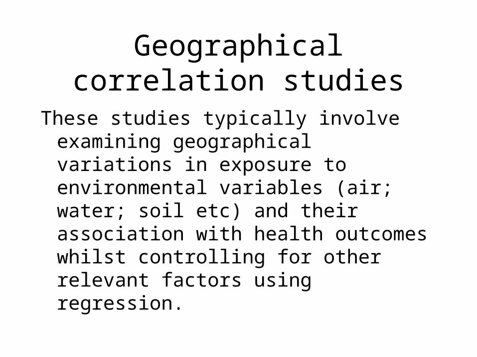
Geographical correlation studies

These studies typically involve examining geographical variations in exposure to environmental variables (air; water; soil etc) and their association with health outcomes whilst controlling for other relevant factors using regression.

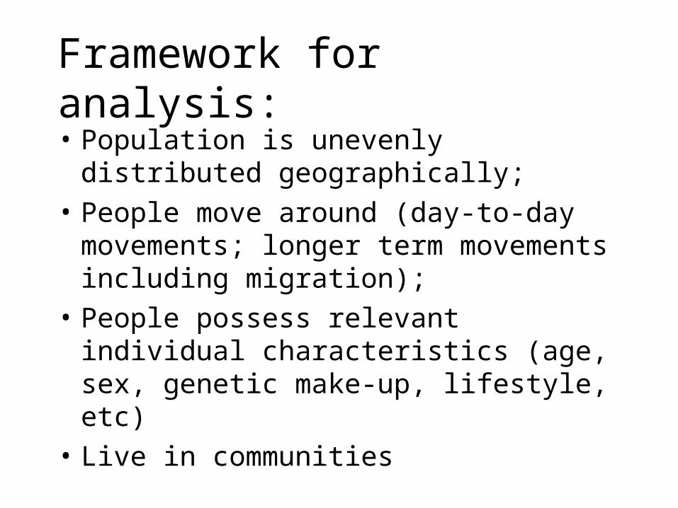
Framework for analysis:

• Population is unevenly distributed geographically;

• People move around (day-to-day movements; longer term movements including migration);

• People possess relevant individual characteristics (age, sex, genetic make-up, lifestyle, etc)

• Live in communities

Problems with small area analyses• Frequency and quality of population data (e.g.

Census every 10 years);• Spatial compatibility of different data sets;• Availability of data on population movements;• Measuring population exposure to the

environmental variable;• Environmental impacts are often likely to be quite

small (relative to, for example, lifestyle effects) and there may be serious confounding effects;

• Cannot estimate strength of an association;• Ecological (or aggregation) bias.

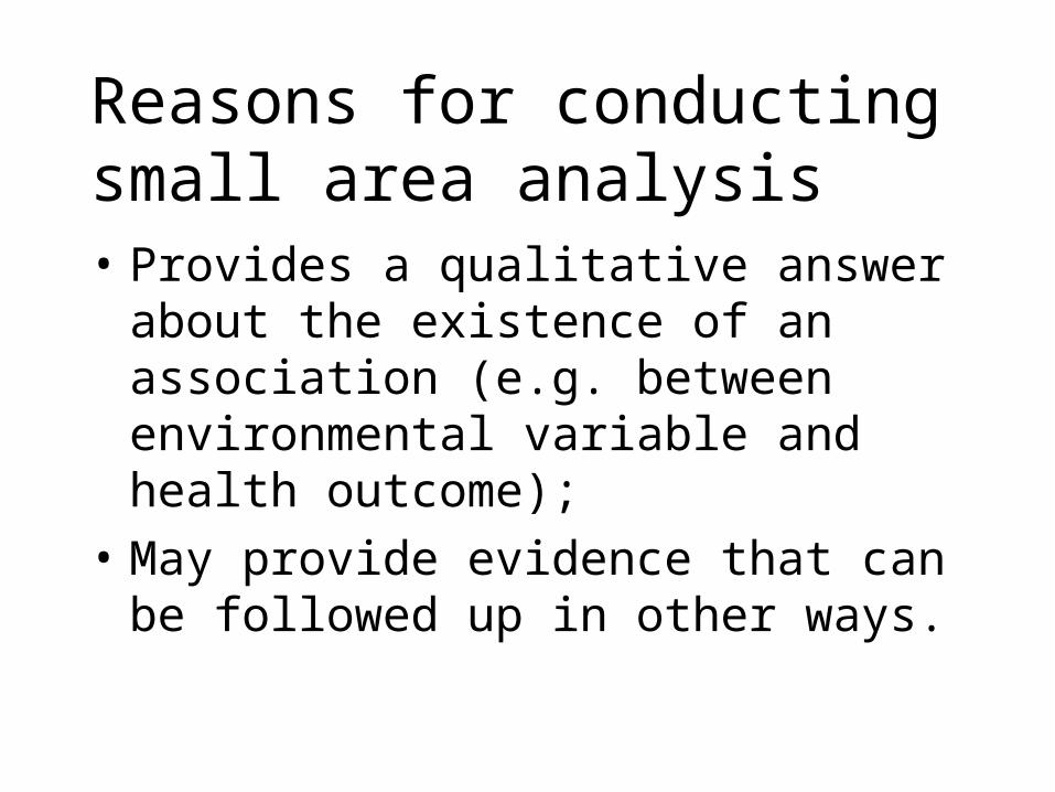
Reasons for conducting small area analysis• Provides a qualitative answer about the

existence of an association (e.g. between environmental variable and health outcome);

• May provide evidence that can be followed up in other ways.

Good practice (Richardson 1992)

• Allow for heterogeneity of exposure;

• Use “well defined” population groups;

• Use survey data to help obtain good exposure data;

• Allow for latency times;

• Allow for population movement effects

Regression model specification:

Oi denotes the number of cases for area i. i = 1,…,n.

If the outcome is rare, typically, it is assumed that Oi is Poisson

distributed with parameter i.

The expected value of Oi is written:

E[Oi] = i = Eiri i = 1, …, n,

where ri is the unknown area-specific relative risk in area i, and Ei

defines the expected number of cases for i given the size of the population and its age and sex composition.

ln[i] = ln[Ei] + ln[ri] .

•This defines a Poisson regression model where is the intercept parameter, and 1, 2,…, k and are regression parameters. ln[Ei] is an

offset.

•The area-specific relative risk at i is associated with attributes of the population X1,…,Xk and the environmental exposure Z at i.

• Adjustment for overdispersion is necessary because of population heterogeneity at the scale of the individual small areas (see, for example, Manton and Stallard 1981).

•Allowance for data uncertainty arising from the use of sample data

ln[i] = ln[Ei] + + 1X1,i +2X2,i + ..... + kXk,i + Zi

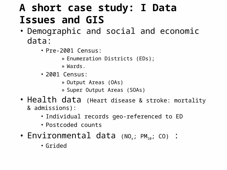
A short case study: I Data Issues and GIS

• Demographic and social and economic data:• Pre-2001 Census:

» Enumeration Districts (EDs);

» Wards.

• 2001 Census:» Output Areas (OAs)

» Super Output Areas (SOAs)

• Health data (Heart disease & stroke: mortality & admissions):

• Individual records geo-referenced to ED

• Postcoded counts

• Environmental data (NOx; PM10; CO) :• Grided

• Problem: obtain a measure of air pollution exposure at the ED level.

Step 1: Measuring NOx exposure. The Indic-Airviro model:

Average annual mean pollution levels 1994-9 (exc 1998): a) NOx (ug/m3) ; b) PM10 (ug/m3)

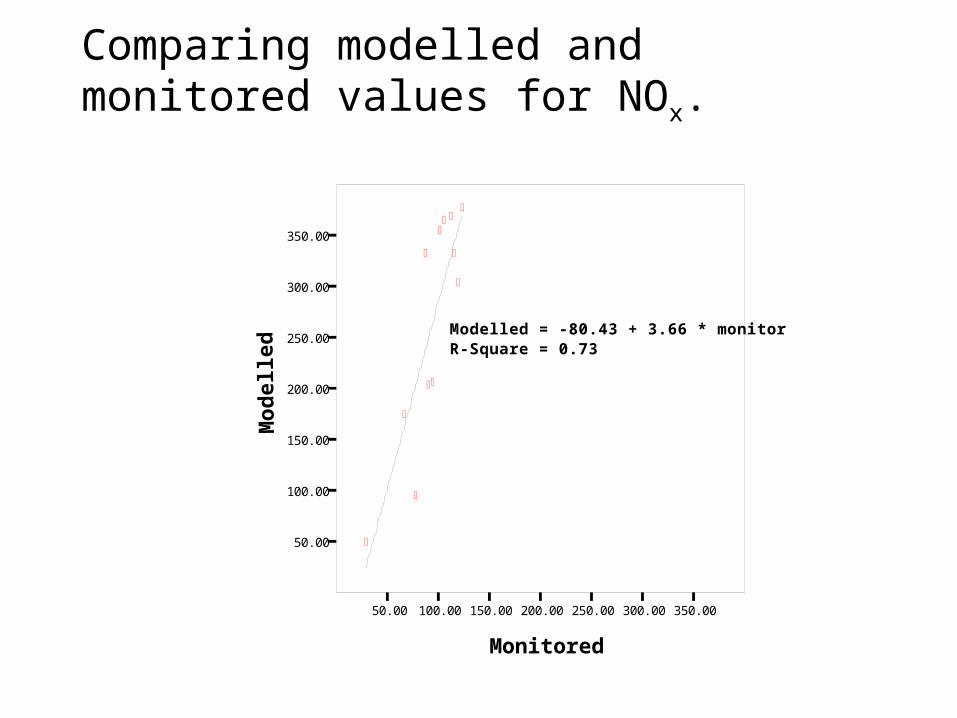
Comparing modelled and monitored values for NOx.

50.00 100.00 150.00 200.00 250.00 300.00 350.00

Monitored

50.00

100.00

150.00

200.00

250.00

300.00

350.00

Mo

del

led

Modelled = -80.43 + 3.66 * monitorR-Square = 0.73

Step 2: Transferring the gridded data to the ED framework. Areal Interpolation: i Area weighting

Areal Interpolation (from grid to EDs): ii point in polygon – ED

centroid

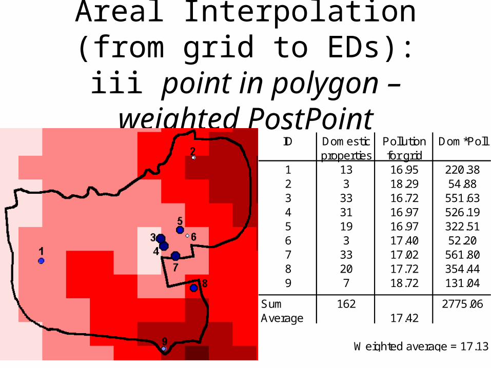
Areal Interpolation (from grid to EDs): iii point in polygon –

weighted PostPointID Domestic Pollution Dom*Poll

properties for grid1 13 16.95 220.382 3 18.29 54.883 33 16.72 551.634 31 16.97 526.195 19 16.97 322.516 3 17.40 52.207 33 17.02 561.808 20 17.72 354.449 7 18.72 131.04

Sum 162 2775.06Average 17.42

Weighted average = 17.13

Weighted PostPoint and ED centroid exposure measures are very similar; areal weighting different

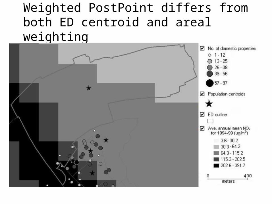
Weighted PostPoint differs from both ED centroid and areal weighting

Where all three methods will give the same or similar results

Step 3: Making allowance for population movements1. Long term population movement:

• Sheffield Health and Illness Prevalence study:– 12,239 representative individuals 18-94 tracked from

1994-2002;– 1491 died; 1572 left Sheffield.– Of the 9176 remaining:

» 70% did not move;» 23% made 1 move» 5% made 2 moves;» Just over 1% made 3 moves» Under 1% made 4 or more moves.

• => significant risk of misclassification of exposure level.

2. Short term population movement

Spatially smoothed CO average of the annual mean pollution levels (1994-1999, excluding 1998) for Sheffield enumeration

districts (ug/m3)(i) 1km; (ii) 2km; (iii) 4km

Comparing indoor and outdoor air pollution exposure

• People spend between 75% and 90% of their time indoors.

• Indoor pollution levels depend not only on outdoor emissions but on housing conditions (cooking, heating, ventilation etc).

• Evidence on relationship between indoor and outdoor pollution levels

Pollutant Source Indoor Outdoor Indoor/outdoor

CO Valerio et al (1997) 7.8 9.55 0.82

NO Drakou et al (1998) 56.53 70.66 0.80

NO2 Drakou et al (1998) 67.14 88.04 0.76

NOx Drakou et al (1998) 126.98 187.74 0.68

O3 Drakou et al (1998) 17.54 37.14 0.47

PM2.5 Lee et al (1997) 25.3 26.3 0.96

PM2.5 Fischer et al (2000) 19.5 23 0.85

PM10 Lee and Chang (2000) 120 134 0.90

PM10 Fischer et al (2000) 29.5 39.5 0.75

    mean (g/m3) mean (g/m3) ratio

SO2 Lee et al (1997) 6.18 11.1 0.56

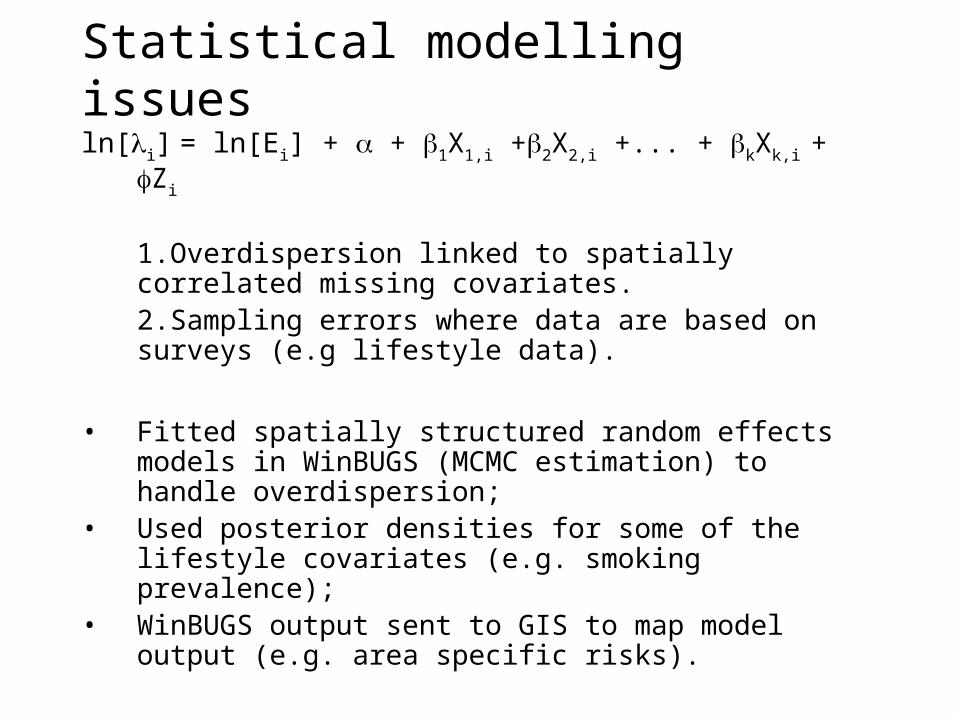
Statistical modelling issues

ln[i] = ln[Ei] + + 1X1,i +2X2,i +... + kXk,i + Zi

1.Overdispersion linked to spatially correlated missing covariates. 2.Sampling errors where data are based on surveys (e.g lifestyle data).

• Fitted spatially structured random effects models in WinBUGS (MCMC estimation) to handle overdispersion;

• Used posterior densities for some of the lifestyle covariates (e.g. smoking prevalence);

• WinBUGS output sent to GIS to map model output (e.g. area specific risks).

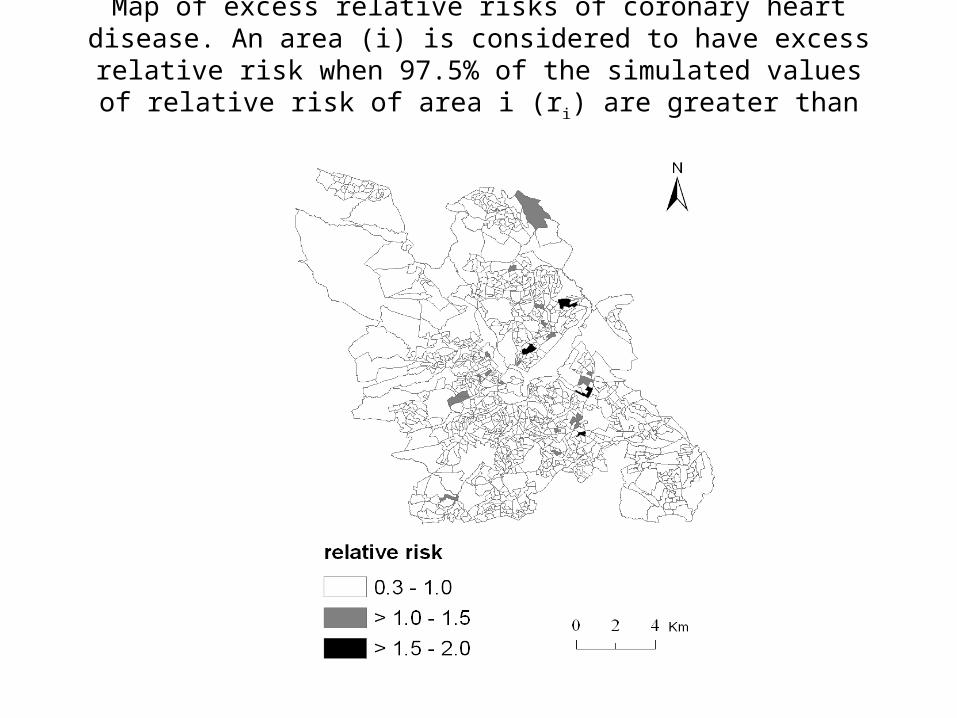
Map of excess relative risks of coronary heart disease. An area (i) is considered to have excess relative risk when 97.5% of the simulated

values of relative risk of area i (ri) are greater than 1.

References:

• P.Brindley, R.Maheswaran, T.Pearson, S.Wise and R.Haining (2004) “Using modelled outdoor air pollution data for health surveillance.” In R.Maheswaran and M.Craglia (eds) GIS in Public Health Practice. Taylor and Francis, London, p.125-149.

• P.Brindley, S.Wise, R.Maheswaran, and R.Haining. (2005) “The effect of alternative representations of population location on the areal interpolation of air pollution exposure.” Computers, Environment and Urban Systems, Vol 29, 455-469.

• R.Maheswaran, R.Haining, P.Brindley, J.Law, T.Pearson, N.Best (2006) “Outdoor NOx and stroke mortality – adjusting for small area level smoking prevalence using a Bayesian approach.” Statistical Methods in Medical Research, 2006, 15, 499-516.