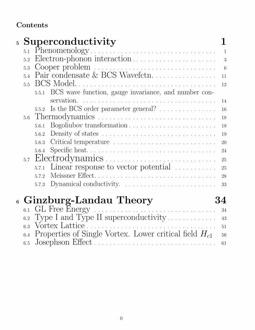
Contents

5 Superconductivity 15.1 Phenomenology . . . . . . . . . . . . . . . . . . . . . . . . . . . . . . . . . 1

5.2 Electron-phonon interaction . . . . . . . . . . . . . . . . . . . . . . 3

5.3 Cooper problem . . . . . . . . . . . . . . . . . . . . . . . . . . . . . . . . 6

5.4 Pair condensate & BCS Wavefctn. . . . . . . . . . . . . . . . . 11

5.5 BCS Model. . . . . . . . . . . . . . . . . . . . . . . . . . . . . . . . . . . . . 12

5.5.1 BCS wave function, gauge invariance, and number con-servation. . . . . . . . . . . . . . . . . . . . . . . . . . . . . . . . . . . . 14

5.5.2 Is the BCS order parameter general? . . . . . . . . . . . . . . . 16

5.6 Thermodynamics . . . . . . . . . . . . . . . . . . . . . . . . . . . . . . . 18

5.6.1 Bogoliubov transformation . . . . . . . . . . . . . . . . . . . . . . . 18

5.6.2 Density of states . . . . . . . . . . . . . . . . . . . . . . . . . . . . . . 19

5.6.3 Critical temperature . . . . . . . . . . . . . . . . . . . . . . . . . . . 20

5.6.4 Specific heat. . . . . . . . . . . . . . . . . . . . . . . . . . . . . . . . . . 24

5.7 Electrodynamics . . . . . . . . . . . . . . . . . . . . . . . . . . . . . 25

5.7.1 Linear response to vector potential . . . . . . . . . . . 25

5.7.2 Meissner Effect. . . . . . . . . . . . . . . . . . . . . . . . . . . . . . . . 28

5.7.3 Dynamical conductivity. . . . . . . . . . . . . . . . . . . . . . . . . 33

6 Ginzburg-Landau Theory 346.1 GL Free Energy . . . . . . . . . . . . . . . . . . . . . . . . . . . . . . . . 34

6.2 Type I and Type II superconductivity . . . . . . . . . . . . . 43

6.3 Vortex Lattice . . . . . . . . . . . . . . . . . . . . . . . . . . . . . . . . . . 51

6.4 Properties of Single Vortex. Lower critical field Hc1 56

6.5 Josephson Effect . . . . . . . . . . . . . . . . . . . . . . . . . . . . . . . . 61

0

5 Superconductivity

5.1 Phenomenology

Superconductivity was discovered in 1911 in the Leiden lab-oratory of Kamerlingh Onnes when a so-called “blue boy”(local high school student recruited for the tedious job of mon-itoring experiments) noticed that the resistivity of Hg metalvanished abruptly at about 4K. Although phenomenologicalmodels with predictive power were developed in the 30’s and40’s, the microscopic mechanism underlying superconductiv-ity was not discovered until 1957 by Bardeen Cooper andSchrieffer. Superconductors have been studied intensively fortheir fundamental interest and for the promise of technologi-cal applications which would be possible if a material whichsuperconducts at room temperature were discovered. Until1986, critical temperatures (Tc’s) at which resistance disap-pears were always less than about 23K. In 1986, Bednorz andMueller published a paper, subsequently recognized with the1987 Nobel prize, for the discovery of a new class of materialswhich currently include members with Tc’s of about 135K.

1

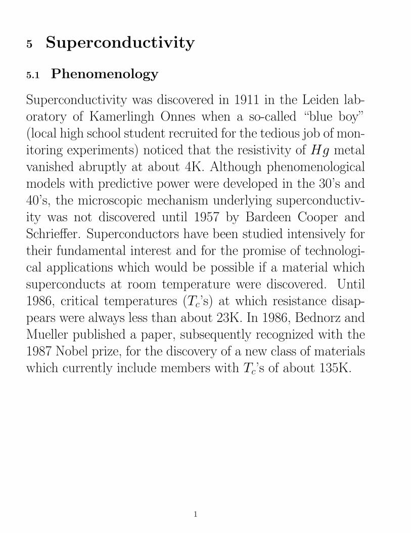
Figure 1: Properties of superconductors.

Superconducting materials exhibit the following unusual be-haviors:

1. Zero resistance. Below a material’s Tc, the DC elec-trical resistivity ρ is really zero, not just very small. Thisleads to the possibility of a related effect,

2. Persistent currents. If a current is set up in a super-conductor with multiply connected topology, e.g. a torus,

2

it will flow forever without any driving voltage. (In prac-tice experiments have been performed in which persistentcurrents flow for several years without signs of degrading).

3. Perfect diamagnetism. A superconductor expels aweak magnetic field nearly completely from its interior(screening currents flow to compensate the field within asurface layer of a few 100 or 1000 A, and the field at thesample surface drops to zero over this layer).

4. Energy gap. Most thermodynamic properties of a su-perconductor are found to vary as e−∆/(kBT ), indicatingthe existence of a gap, or energy interval with no allowedeigenenergies, in the energy spectrum. Idea: when thereis a gap, only an exponentially small number of particleshave enough thermal energy to be promoted to the avail-able unoccupied states above the gap. In addition, this gapis visible in electromagnetic absorption: send in a photonat low temperatures (strictly speaking, T = 0), and noabsorption is possible until the photon energy reaches 2∆,i.e. until the energy required to break a pair is available.

5.2 Electron-phonon interaction

Superconductivity is due to an effective attraction betweenconduction electrons. Since two electrons experience a re-pulsive Coulomb force, there must be an additional attrac-tive force between two electrons when they are placed in ametallic environment. In classic superconductors, this force

3

is known to arise from the interaction with the ionic system.In previous discussion of a normal metal, the ions were re-placed by a homogeneous positive background which enforcescharge neutrality in the system. In reality, this medium ispolarizable– the number of ions per unit volume can fluctuatein time. In particular, if we imagine a snapshot of a singleelectron entering a region of the metal, it will create a netpositive charge density near itself by attracting the oppositelycharged ions. Crucial here is that a typical electron close tothe Fermi surface moves with velocity vF = ~kF/m which ismuch larger than the velocity of the ions, vI = VFm/M . Soby the time (τ ∼ 2π/ωD ∼ 10−13 sec) the ions have polarizedthemselves, 1st electron is long gone (it’s moved a distance

vFτ ∼ 108cm/s ∼ 1000A, and 2nd electron can happen by

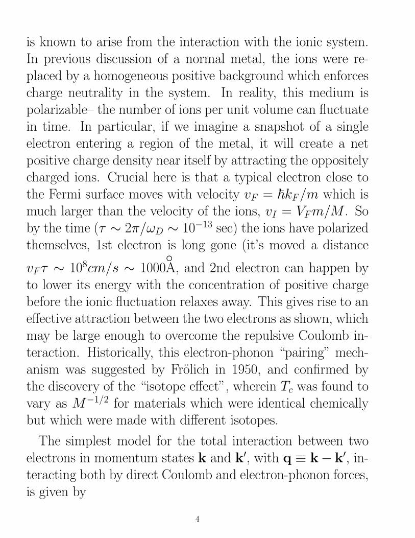
to lower its energy with the concentration of positive chargebefore the ionic fluctuation relaxes away. This gives rise to aneffective attraction between the two electrons as shown, whichmay be large enough to overcome the repulsive Coulomb in-teraction. Historically, this electron-phonon “pairing” mech-anism was suggested by Frolich in 1950, and confirmed bythe discovery of the “isotope effect”, wherein Tc was found tovary as M−1/2 for materials which were identical chemicallybut which were made with different isotopes.

The simplest model for the total interaction between twoelectrons in momentum states k and k′, with q ≡ k− k′, in-teracting both by direct Coulomb and electron-phonon forces,is given by

4

Figure 2: Effective attraction of two electrons due to “phonon exchange”

V (q, ω) =4πe2

q2 + k2s+

4πe2

q2 + k2s

ω2q

ω2 − ω2q

, (1)

in the jellium model. Here first term is Coulomb interac-tion in the presence of a medium with dielectric constantε = 1+k2s/q

2, and ωq are the phonon frequencies. The screen-ing length k−1

s is 1A or so in a good metal. Second term isinteraction due to exchange of phonons, i.e. the mechanismpictured in the figure. Note it is frequency-dependent, re-flecting the retarded nature of interaction (see figure), and inparticular that the 2nd term is attractive for ω < ωq ∼ ωD.Something is not quite right here, however; it looks indeedas though the two terms are of the same order as ω → 0;indeed they cancel each other there, and V is seen to be al-ways repulsive. This indicates that the jellium approximationis too simple. We should probably think about a more care-ful calculation in a real system as producing two equivalentterms, which vary in approximately the same way with kTFand ωq, but with prefactors which are arbitrary. In some ma-terials, then, the second term might “win” at low frequencies,depending on details. The BCS interaction is sometimes re-

5

ferred to as a “residual” attractive interaction, i.e. what isleft when the long-range Coulomb

5.3 Cooper problem

A great deal was known about the phenomenology of super-conductivity in the 1950’s, and it was already suspected thatthe electron phonon interaction was responsible, but the mi-croscopic form of the wave function was unknown. A cluewas provided by Leon Cooper, who showed that the noninter-acting Fermi sea is unstable towards the addition of a singlepair of electrons with attractive interactions. Cooper beganby examining the wave function of this pair ψ(r1, r2), whichcan always be written as a sum over plane waves

ψ(r1, r2) =∑

kq

uk(q)eik·r1e−i(k+q)·r2ζ (2)

where the uk(q) are expansion coefficients and ζ is the spinpart of the wave function, either the singlet | ↑↓ − ↓↑> /

√2

or one of the triplet, | ↑↑>, | ↓↓>, | ↑↓ + ↓↑> /√2. In

fact since we will demand that ψ is the ground state of thetwo-electron system, we will assume the wave function is re-alized with zero center of mass momentum of the two elec-trons, uk(q) = ukδq,0. Here is a quick argument related tothe electron-phonon origin of the attractive interaction.1 Theelectron-phonon interaction is strongest for those electronswith single-particle energies ξk within ωD of the Fermi level.

1Thanks to Kevin McCarthy, who forced me to think about this further

6

k

p

-q

k-q p+q

k p

g gωD

p+q

k-q

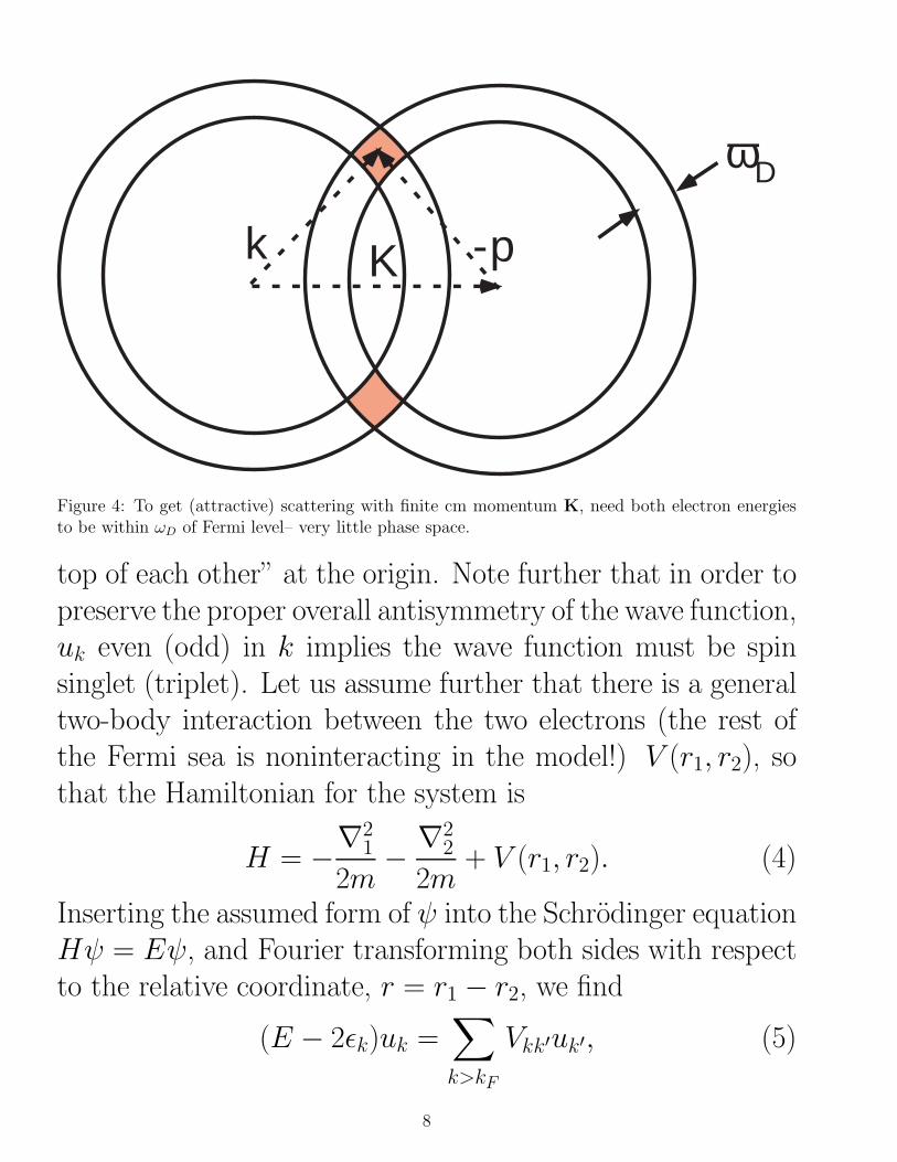
Figure 3: Electrons scattered by phonon exchange are confined to shell of thickness ωD about Fermisurface.

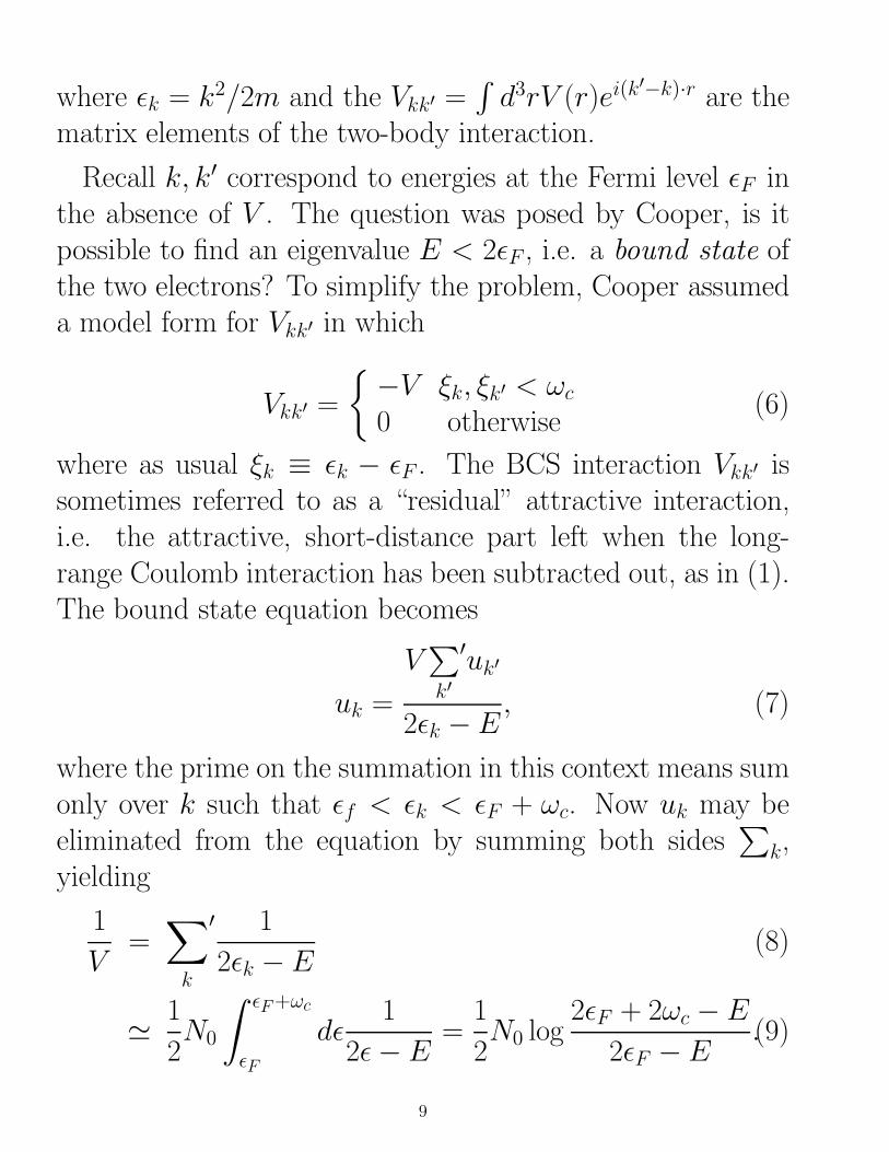
In the scattering process depicted in Fig. 3, momentum isexplicitly conserved, i.e. the total momentum

k + p = K (3)

is the same in the incoming and outgoing parts of the diagram.Now look at Figure 4, and note that ifK is not∼ 0, the phasespace for scattering (attraction) is dramatically reduced. Sothe system can always lower its energy by creating K = 0pairs. Henceforth we will make this assumption, as Cooperdid.

Then ψ(r1, r2) becomes∑

k ukeik·(r1−r2). Note that if uk is

even in k, the wave function has only terms ∝ cos k ·(r1−r2),whereas if it is odd, only the sin k · (r1 − r2) will contribute.This is an important distinction, because only in the formercase is there an amplitude for the two electrons to live ”on

7

-pKk

ωD

Figure 4: To get (attractive) scattering with finite cm momentum K, need both electron energiesto be within ωD of Fermi level– very little phase space.

top of each other” at the origin. Note further that in order topreserve the proper overall antisymmetry of the wave function,uk even (odd) in k implies the wave function must be spinsinglet (triplet). Let us assume further that there is a generaltwo-body interaction between the two electrons (the rest ofthe Fermi sea is noninteracting in the model!) V (r1, r2), sothat the Hamiltonian for the system is

H = −∇21

2m− ∇2

2

2m+ V (r1, r2). (4)

Inserting the assumed form of ψ into the Schrodinger equationHψ = Eψ, and Fourier transforming both sides with respectto the relative coordinate, r = r1 − r2, we find

(E − 2εk)uk =∑

k>kF

Vkk′uk′, (5)

8

where εk = k2/2m and the Vkk′ =∫d3rV (r)ei(k

′−k)·r are thematrix elements of the two-body interaction.

Recall k, k′ correspond to energies at the Fermi level εF inthe absence of V . The question was posed by Cooper, is itpossible to find an eigenvalue E < 2εF , i.e. a bound state ofthe two electrons? To simplify the problem, Cooper assumeda model form for Vkk′ in which

Vkk′ =

−V ξk, ξk′ < ωc0 otherwise

(6)

where as usual ξk ≡ εk − εF . The BCS interaction Vkk′ issometimes referred to as a “residual” attractive interaction,i.e. the attractive, short-distance part left when the long-range Coulomb interaction has been subtracted out, as in (1).The bound state equation becomes

uk =

V∑

k′

′uk′

2εk − E, (7)

where the prime on the summation in this context means sumonly over k such that εf < εk < εF + ωc. Now uk may beeliminated from the equation by summing both sides

∑

k,yielding

1

V=

∑

k

′ 1

2εk − E(8)

' 1

2N0

∫ εF+ωc

εF

dε1

2ε− E=

1

2N0 log

2εF + 2ωc − E

2εF − E.(9)

9

For a weak interaction N0V 1, we expect a solution (if atall) just below the Fermi level, so we treat 2εF −E as a smallpositive quantity, e.g. negligible compared to 2ωc. We thenarrive at the pair binding energy

∆Cooper ≡ 2εF − E ' 2ωce−2/N0V . (10)

There are several remarks to be made about this result.

1. Note (for your own information–Cooper didn’t know thisat the time!) that the dependence of the bound state en-ergy on both the interaction V and the cutoff frequency ωcstrongly resembles the famous BCS transition temperaturedependence, with ωc identified as the phonon frequencyωD, as given in equation (I.1).

2. the dependence on V is that of an essential singularity,i.e. a nonanalytic function of the parameter. Thus wemay expect never to arrive at this result at any order inperturbation theory, an unexpected problem which hin-dered theoretical progress for a long time.

3. The solution found has isotropic or s-symmetry, since itdoesn’t depend on the k on the Fermi surface. (How wouldan angular dependence arise? Look back over the calcula-tion.)

4. Note the integrand (2εk−E)−1 = (2ξk+∆Cooper)−1 peaks

at the Fermi level with energy spread ∆Cooper of statesinvolved in the pairing. The weak-coupling (N0V 1)solution therefore provides a bit of a posteriori justifica-tion for its own existence, since the fact that ∆Cooper ωc

10

implies that the dependence of Vkk′ on energies out nearthe cutoff and beyond is in fact not terribly important, sothe cutoff procedure used was ok.

5. The spread in momentum is therefore roughly ∆Cooper/vF ,and the characteristic size of the pair (using Heisenberg’suncertainty relation) about vF/Tc. This is about 100-1000A in metals, so since there is of order 1 electron/ unitcell in a metal, and if this toy calculation has anythingto do with superconductivity, there are certainly manyelectron pairs overlapping each other in real space in asuperconductor.

5.4 Pair condensate & BCS Wavefctn.

Obviously one thing is missing from Cooper’s picture: if it isenergetically favorable for two electrons in the presence of anoninteracting Fermi sea to pair, i.e. to form a bound state,why not have the other electrons pair too, and lower the en-ergy of the system still further? This is an instability of thenormal state, just like magnetism or charge density wave for-mation, where a ground state of completely different charac-ter (and symmetry) than the Fermi liquid is stabilized. TheCooper calculation is a T=0 problem, but we expect that asone lowers the temperature, it will become at some criticaltemperature Tc energetically favorable for all the electrons topair. Although this picture is appealing, many things aboutit are unclear: does the pairing of many other electrons alter

11

the attractive interaction which led to the pairing in the firstplace? Does the bound state energy per pair change? Do allof the electrons in the Fermi sea participate? And most im-portantly, how does the critical temperature actually dependon the parameters and can we calculate it?

5.5 BCS Model.

A consistent theory of superconductivity may be constructedeither using the full “effective interaction” or our approxima-tion V (q, ω) to it. However almost all interesting questionscan be answered by the even simpler model used by BCS.The essential point is to have an attractive interaction forelectrons in a shell near the Fermi surface; retardation is sec-ondary. Therefore BCS proposed starting from a phenomeno-logical Hamiltonian describing free electrons scattering via aneffective instantaneous interaction a la Cooper:

H = H0 − V∑

kk′qσσ′

′c†kσc

†−k+qσ′c−k′+qσ′ck′σ, (11)

where the prime on the sum indicates that the energies of thestates k and k′ must lie in the shell of thickness ωD. Note theinteraction term is just the Fourier transform of a completelylocal 4-Fermi interaction ψ†(r)ψ†(r)ψ(r)ψ(r).2

Recall that in our discussion of the instability of the nor-mal state, we suggested that an infinitesimal pair field could

2Note this is not the most general form leading to superconductivity. Pairing in higher angular momentumchannels requires a bilocal model Hamiltonian, as we shall see later.

12

produce a finite amplitude for pairing. That amplitude wasthe expectation value 〈c†kσc

†−k−σ〉. We ignore for the moment

the problems with number conservation, and ask if we cansimplify the Hamiltonian still further with a mean field ap-proximation, again to be justified a posteriori. We proceedalong the lines of generalized Hartree-Fock theory, and rewritethe interaction as

c†kσc†−k+qσ′c−k′+qσ′ck′σ = [〈c†kσc

†−k+qσ′〉 + δ(c†c†)]×

×[〈c−k′+qσ′ck′σ〉 + δ(cc)], (12)

where, e.g. δ(cc) = c−k′+qσ′ck′σ − 〈c−k′+qσ′ck′σ〉 is the fluctu-ation of this operator about its expectation value. If a meanfield description is to be valid, we should be able to neglectterms quadratic in the fluctuations when we expand Eq (20).If we furthermore make the assumption that pairing will takeplace in a uniform state (zero pair center of mass momentum),then we put 〈c−k′+qσ′ck′σ〉 = 〈c−k′σ′ck′σ〉δq,0. The effectiveHamiltonian then becomes (check!)

H ' H0 − (∆∑

k

c†k↑c†−k↓ + h.c.) + ∆〈c†k↑c

†−k↓〉∗, (13)

where∆ = V

∑

k

′〈c−k↓ck↑〉. (14)

What BCS (actually Bogoliubov, after BCS) did was then totreat the order parameter ∆ as a (complex) number, andcalculate expectation values in the approximate Hamiltonian(13), insisting that ∆ be determined self-consistently via Eq.

13

(14) at the same time.3

5.5.1 BCS wave function, gauge invariance, and number con-

servation.

What BCS actually did in their original paper is to treat theHamiltonian (11) variationally. Their ansatz for the groundstate of (11) is a trial state with the pairs k ↑,−k ↓ occupiedwith amplitude vk and unoccupied with amplitude uk, suchthat |uk|2 + |vk|2 = 1:

|ψ >= Πk(uk + vkc†k↑c

†−k↓)|0 > . (15)

This is a variational wave function, so the energy is to beminimized over the space of uk, vk. Alternatively, one candiagonalize the Hartree-Fock (BCS) Hamiltonian directly, to-gether with the self-consistency equation for the order param-eter; the two methods turn out to be equivalent. I will followthe latter procedure, but first make a few remarks on the formof the wave function. First, note the explicit violation of par-ticle number conservation: |ψ > is a superposition of statesdescribing 0, 2, 4 , N-particle systems.4 In general a quan-tum mechanical system with fixed particle number N (like,e.g. a real superconductor!) manifests a global U (1) gauge

symmetry, because H is invariant under c†kσ → eiθc†kσ. Thestate |ψ > is characterized by a set of coefficients uk, vk,which becomes uk, e2iθvk after the gauge transformation.

3If the pairing interaction is momentum dependent the self-consistency or “gap” equation reads ∆k =∑′

k′ Vkk′〈c−k′↓ck′↑〉, which reduces to (14) if one sets Vkk′ = V .4What happened to the odd numbers? In mesoscopic superconductors, there are actually differences in the

properties of even and odd-number particle systems, but for bulk systems the distinction is irrelevant.

14

The two states |ψ > and ψ(φ), where φ = 2θ, are inequiva-lent, mutually orthogonal quantum states, since they are notsimply related by a multiplicative phase factor.5 Since His independent of φ, however, all states |ψ(φ) > are contin-uously degenerate, i.e. the ground state has a U (1) gauge(phase) symmetry. Any state |ψ(φ) > is said to be a bro-ken symmetry state, becaue it is not invariant under a U (1)transformation, i.e. the system has ”chosen” a particular φout of the degenerate range 0 < φ < 2π. Nevertheless the ab-solute value of the overall phase of the ground state is not anobservable, but its variations δφ(r, t) in space and time are.It is the rigidity of the phase, i.e. the energy cost of any ofthese fluctuations, which is responsible for superconductivity.

Earlier I mentioned that it was possible to construct a num-ber conserving theory. It is now instructive to see how: statesof definite number are formed [Anderson 1958] by making co-herent superpositions of states of definite phase

|ψ(N) >=

∫ 2π

0

dφeiφN/2|ψ(φ) > . (16)

[The integration over φ gives zero unless there are in the ex-pansion of the product contained in |ψ > precisely N/2 paircreation terms, each with factor exp iφ.] Note while this statehas maximal uncertainty in the value of the phase, the rigidityof the system to phase fluctuations is retained.6

5In the normal state, |ψ > and ψ(φ) differ by a global multiplicative phase eiθ, which has no physical consequences,and the ground state is nondegenerate.

6The phase and number are in fact canonically conjugate variables, [N/2, φ] = i, where N = 2i∂/∂φ in the φrepresentation.

15

It is now straightforward to see why BCS theory works.The BCS wave function |ψ > may be expressed as a sum|ψ >=

∑

N aN |ψ(N) > [Convince yourself of this by calcu-lating the aN explicitly!]. IF we can show that the distribu-tion of coefficients aN is sharply peaked about its mean value< N >, then we will get essentially the same answers as work-ing with a state of definite number N =< N >. Using theexplicit form (15), it is easy to show

〈N〉 = 〈ψ|∑

kσ

nkσ|ψ〉 = 2∑

k

|vk|2 ; 〈(N−〈N〉)2〉 =∑

k

u2kv2k.

(17)Now the uk and vk will typically be numbers of order 1, sosince the numbers of allowed k-states appearing in the k sumsscale with the volume of the system, we have 〈N〉 ∼ V , and〈(N−〈N〉)2〉 ∼ V . Therefore the width of the distribution ofnumbers in the BCS state is 〈(N − 〈N〉)2〉1/2/〈N〉 ∼ N−1/2.As N → 1023 particles, this relative error implied by thenumber nonconservation in the BCS state becomes negligible.

5.5.2 Is the BCS order parameter general?

Before leaving the subject of the phase in this section, it isworthwhile asking again why we decided to pair states withopposite momenta and spin, k ↑ and −k ↓. The BCS argu-ment had to do 1) with minimizing the energy of the entiresystem by giving the Cooper pairs zero center of mass mo-mentum, and 2) insisting on a spin singlet state because thephonon mechanism leads to electron attraction when the elec-

16

trons are at the same spatial position (because it is retardedin time!), and a spatially symmetric wavefunction with largeamplitude at the origin demands an antisymmetric spin part.Can we relax these assumptions at all? The first require-ment seems fairly general, but it should be recalled that onecan couple to the pair center of mass with an external mag-netic field, so that one will create spatially inhomogeneous(finite-q) states with current flow in the presence of a mag-netic field. Even in zero external field, it has been proposedthat systems with coexisting antiferromagnetic correlationscould have pairing with finite antiferromagnetic nesting vec-tor ~Q [Baltensberger and Strassler 1963]. The requirementfor singlet pairing can clearly be relaxed if there is a pair-ing mechanism which disfavors close approach of the pairedparticles. This is the case in superfluid 3He, where the hardcore repulsion of two 3He atoms supresses Tc for s-wave, sin-glet pairing and enhances Tc for p-wave, triplet pairing wherethe amplitude for two particles to be together at the origin isalways zero.

In general, pairing is possible for some pair mechanism ifthe single particle energies corresponding to the states kσ andk′σ′ are degenerate, since in this case the pairing interactionis most attractive. In the BCS case, a guarantee of this degen-eracy for k ↑ and −k ↓ in zero field is provided by Kramer’stheorem, which says these states must be degenerate becausethey are connected by time reversal symmetry. However,there are other symmetries: in a system with inversion sym-

17

metry, parity will provide another type of degeneracy, so k ↑,k ↓, −k ↑ and −k ↓ are all degenerate and may be pairedwith one another if allowed by the pair interaction.

5.6 Thermodynamics

5.6.1 Bogoliubov transformation

We now return to (13) and discuss the solution by canonicaltransformation given by Bogoliubov. After our drastic ap-proximation, we are left with a quadratic Hamiltonian in thec’s, but with c†c† and cc terms in addition to c†c’s. We can di-agonalize it easily, however, by introducing the quasiparticleoperators γk0 and γk1 by

ck↑ = u∗kγk0 + vkγ†k1

c†−k↓ = −v∗kγk0 + ukγ†k1. (18)

You may check that this transformation is canonical (preservesfermion comm. rels.) if |uk|2 + |vk|2 = 1. Substituting into(13) and using the commutation relations we get

HBCS =∑

k

ξk[(|uk|2 − |vk|2)(γ†k0γk0 + γ†k1γk1) + 2|vk|2

+2u∗kv∗kγk1γk0 + 2ukvkγ

†k1γ

†k0]

+∑

k

[(∆kukv∗k +∆∗

ku∗kvk)(γ

†k0γk0 + γ†k1γk1 − 1)

+(∆kv∗2k −∆∗

ku∗2k )γk1γk0 + (∆∗

kv2k −∆ku

2k)γ

†k0γ

†k1

+∆k〈c†k↑c†−k↓〉∗, (19)

18

which does not seem to be enormous progress, to say the least.But the game is to eliminate the terms which are not of theform γ†γ, so to be left with a sum of independent number-typeterms whose eigenvalues we can write down. The coefficientsof the γ†γ† and γγ type terms are seen to vanish if we choose

2ξkukvk +∆∗kv

2k −∆ku

2k = 0. (20)

This condition and the normalization condition |uk|2+|vk|2 =1 are both satisfied by the solutions

|uk|2|vk|2

=1

2

(

1± ξkEk

)

, (21)

where I defined the Bogolibov quasiparticle energy

Ek =√

ξ2k + |∆k|2. (22)

The BCS Hamiltonian has now been diagonalized:

HBCS =∑

k

Ek

(

γ†k0γk0 + γ†k1γk1)

+∑

k

(

ξk − Ek +∆k〈c†k↑c†−k↓〉∗

)

.

(23)Note the second term is just a constant, which will be impor-tant for calculating the ground state energy accurately. Thefirst term, however, just describes a set of free fermion exci-tations above the ground state, with spectrum Ek.

5.6.2 Density of states

The Bogoliubov quasiparticle spectrum Ek is easily seen tohave a minimum ∆k for a given direction k on the Fermi sur-face defined by ξk = 0; ∆k therefore, in addition to playing

19

the role of order parameter for the superconducting transi-tion, is also the energy gap in the 1-particle spectrum. Tosee this explicitly, we can simply do a change of variables inall energy integrals from the normal metal eigenenergies ξk tothe quasiparticle energies Ek:

N(E)dE = NN(ξ)dξ. (24)

If we are interested in the standard case where the gap ∆ ismuch smaller than the energy over which the normal state dosNN(ξ) varies near the Fermi level, we can make the replace-ment

NN(ξ) ' NN(0) ≡ N0, (25)

so using the form of Ek from (22) we find

N(E)

N0=

E√E2−∆2 E > ∆

0 E < ∆. (26)

This function is sketched in Figure 5.

5.6.3 Critical temperature

The critical temperature is defined as the temperature atwhich the order parameter ∆k vanishes. We can now cal-culate this with the aid of the diagonalized Hamiltonian. The

20

N(E)

N 0

E

Normal

SC

10

1

ξ

ξ || ξ ||

energy

Ε

∆

Figure 5: a) Normalized density of states; b) Quasiparticle spectrum.

self-consistency condition is

∆∗k = V

∑

k′〈c†

k′↑c†−k′↓〉

∗

= V∑

k′uk′v

∗k′〈1− γ†k0γk0 − γ†k1γk1〉

= V∑

k

∆∗k

2Ek

(1− 2f(Ek)) . (27)

Since 1 − 2f(E) = tanh[E/(2T )], the BCS gap equation

reads

∆∗k = V

∑

k′

∆∗k′

2Ek′tanh

Ek′

2T(28)

This equation may now be solved, first for the critical temper-ature itself, i.e. the temperature at which ∆ → 0, and thenfor the normalized order parameter ∆/Tc for any temperatureT . It is the ability to eliminate all normal state parameters

21

from the equation in favor of Tc itself which makes the BCStheory powerful. For in practice the parameters ωD, N0, andparticularly V are known quite poorly, and the fact that twoof them occur in an exponential makes an accurate first prin-ciples calculation of Tc nearly impossible. You should alwaysbe suspicious of a theory which claims to be able to calculateTc! On the other hand, Tc is easy to measure, so if it is theonly energy scale in the theory, we have a tool with enormouspredictive power.

First note that at Tc, the gap equation becomes

1

N0V=

∫ ωD

0

dξk1

ξktanh

ξk2Tc

. (29)

This integral can be approximated carefully, but it is usefulto get a sense of what is going on by doing a crude treatment.Note that since Tc ωD generally, most of the integrandweight occurs for ξ > T , so we can estimate the tanh factorby 1. The integral is log divergent, which is why the cutoffωD is so important. We find

1

N0V0= log

ω

Tc⇒ Tc ' ωDe

−1/N0V (30)

The more accurate analysis of the integral gives the BCS result

Tc = 1.14ωDe−1/N0V (31)

We can do the same calculation near Tc, expanding to lead-ing order in the small quantity ∆(T )/T , to find ∆(T )/Tc '

22

3.06(1− T/Tc)1/2. At T = 0 we have

1

N0V=

∫ ωD

0

dξk1

Ek=

∫ ωD

∆

dEN(E)/E (32)

=

∫ ωD

∆

dE1√

E2 −∆2' ln(2ωd/∆), (33)

so that ∆(0) ' 2ωD exp−1/N0V , or ∆(0)/Tc ' 1.76. Thefull temperature dependence of ∆(T ) is sketched in Figure 6).In the halcyon days of superconductivity theory, comparisons

∆

TTc

(T)1.76 Tc

Figure 6: BCS order parameter as fctn. of T .

with the theory had to be compared with a careful table of∆/Tc painstakingly calculated and compiled by Muhlschlegl.Nowadays the numerical solution requires a few seconds ona PC. It is frequently even easier to use a phenomenologicalapproximate closed form of the gap, which is correct nearT = 0 and = Tc:

∆(T ) = δscTctanhπ

δsc

√

aδC

CN(TcT

− 1), (34)

23

where δsc = ∆(0)/Tc = 1.76, a = 2/3, and δC/CN = 1.43is the normalized specific heat jump.7 This is another of the“universal” ratios which the BCS theory predicted and whichhelped confirm the theory in classic superconductors.

5.6.4 Specific heat.

The gap in the density of states is reflected in all thermody-namic quantities as an activated behavior e−∆/T , at low T ,due to the exponentially small number of Bogoliubov quasi-particles with thermal energy sufficient to be excited over thegap ∆ at low temperatures T ∆. The electronic specificheat is particularly easy to calculate, since the entropy of theBCS superconductor is once again the entropy of a free gasof noninteracting quasiparticles, with modified spectrum Ek.The expression (II.6) then gives the entropy directly, and maybe rewritten

S = −kB∫ ∞

0

dEN(E)f(E)lnf(E)+[1−f(E)]ln[1−f(E)],(35)

where f(E) is the Fermi function. The constant volume spe-cific heat is just Cel,V = T [dS/dT ]V , which after a little alge-bra may be written

Cel,V =2

T

∫

dEN(E)(−∂f∂E

)[E2 − 1

2Td∆2

dT]. (36)

A sketch of the result of a full numerical evaluation is shownin Figure 1. Note the discontinuity at Tc and the very rapid

7Note to evaluate the last quantity, we need only use the calculated temperature dependence of ∆ near Tc, andinsert into Eq. (47).

24

falloff at low temperatures.

It is instructive to actually calculate the entropy and specificheat both at low temperatures and near Tc. For T ∆,f(E) ' e−E/T and the density of states factor N(E) in theintegral cuts off the integration at the lower limit ∆, givingC ' (N0∆

5/2/T 3/2)e−∆/T .8

Note the first term in Eq. (47)is continuous through thetransition ∆ → 0 (and reduces to the normal state specificheat (2π2/3)N0T above Tc), but the second one gives a dis-continuity at Tc of (CN−CS)/CN = 1.43, where CS = C(T−

c )and CN = C(T+

c ). To evaluate (36), we need the T depen-dence of the order parameter from a general solution of (28).

5.7 Electrodynamics

5.7.1 Linear response to vector potential

The existence of an energy gap is not a sufficient condition forsuperconductivity (actually, it is not even a necessary one!).Insulators, for example, do not possess the phase rigidity

which leads to perfect conductivity and perfect diamagnetismwhich are the defining characteristics of superconductivity.We can understand both properties by calculating the cur-

8To obtain this, try the following:

• replace the derivative of Fermi function by exp-E/T

• do integral by parts to remove singularity at Delta

• expand around Delta E = Delta + delta E

• change integration variables from E to delta E

Somebody please check my answer!

25

rent response of the system to an applied magnetic or electricfield.9 The kinetic energy in the presence of an applied vectorpotential A is just

H0 =1

2m

∑

σ

∫

d3rψ†σ(r)[−i∇− (

e

c)A]2ψσ(r), (37)

and the second quantized current density operator is given by

j(r) =e

2mψ†(r)(−i∇− e

cA)ψ(r) + [(i∇− e

cA)ψ†(r)]ψ(r) (38)

= jpara −e2

mcψ†(r)ψ(r)A, (39)

where

jpara(r) =−ie2m

ψ†(r)∇ψ(r)− (∇ψ†(r))ψ(r), (40)

or in Fourier space,

jpara(q) =e

m

∑

kσ

kc†k−qσckσ (41)

We would like to do a calculation of the linear current re-sponse j(q, ω) to the application of an external field A(q, ω)to the system a long time after the perturbation is turnedon. Expanding the Hamiltonian to first order in A gives theinteraction

H ′ =

∫

d3rjpara ·A =e

mc

∑

kσ

k ·A(q)c†k−qσcqσ. (42)

9To see this, note that we can choose a gauge where E = −(1/c)∂A/∂t = −iωA/c for a periodic electric field.Then the Fourier component of the current is

j(q, ω) = σ(q, ω)E(q, ω) = K(q, ω)A(q, ω),

so σ(q, ω) = icK(q, ω)/ω.

26

The expectation value < j > may now be calculated to linearorder via the Kubo formula, yielding

〈j〉(q, ω) = K(q, ω)A(q, ω) (43)

with

K(q, ω) = −ne2

mc+ 〈[jpara, jpara]〉(q, ω). (44)

Note the first term in the current

jdia(q, ω) ≡ −ne2

mcA(q, ω) (45)

is purely diagmagnetic, i.e. these currents tend to screen theexternal field (note sign). The second, paramagnetic term isformally the Fourier transform of the current-current corre-lation function (correlation function used in the sense of ourdiscussion of the Kubo formula).10 Here are a few remarks onthis expression:

• Note the simple product structure of (43) in momentumspace implies a nonlocal relationship in general between j

and A., i.e. j(r) depends on the A(r′) at many points r′

around r.11

• Note also that the electric field in a gauge where the elec-trostatic potential is set to zero may be written E(q, ω) =

10We will see that the first term gives the diamagnetic response of the system, and the second the temperature-dependent paramagnetic response.

11If we transformed back, we’d get the convolution

j(r) =

∫

d3r′K(r, r′)A(r′) (46)

27

−iωA(q, ω), so that the complex conductivity of the sys-tem defined by j = σE may be written

σ(q, ω) =i

ωK(q, ω) (47)

• What happens in a normal metal? The paramagnetic sec-ond term cancels the diamagnetic response at ω = 0,leaving no real part of K (Im part of σ), i.e. the conduc-tivity is purely dissipative and not inductive at ω,q = 0in the normal metal.

5.7.2 Meissner Effect.

There is a theorem of classical physics proved by Bohr12 whichstates that the ground state of a system of charged particlesin an external magnetic field carries zero current. The essen-tial element in the proof of this theorem is the fact that themagnetic forces on the particles are always perpendicular totheir velocities. In a quantum mechanical system, the threecomponents of the velocity do not commute in the presenceof the field, allowing for a finite current to be created in theground state. Thus the existence of the Meissner effect insuperconductors, wherein magnetic flux is expelled from theinterior of a sample below its critical temperature, is a clearproof that superconductivity is a manifestation of quantummechanics.

12See “The development of the quantum-mechanical electron theory of metals: 1928-33.” L. Hoddeson and G.Baym, Rev. Mod. Phys., 59, 287 (1987).

28

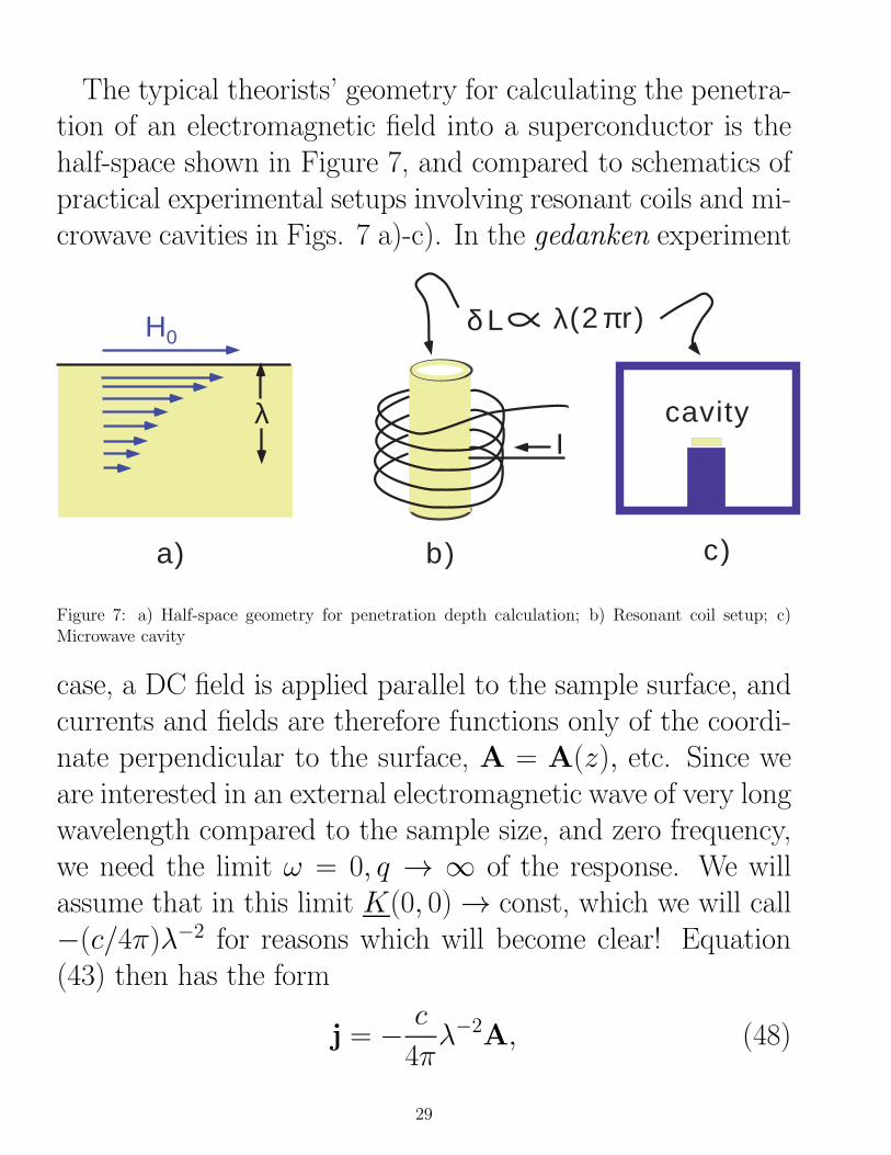
The typical theorists’ geometry for calculating the penetra-tion of an electromagnetic field into a superconductor is thehalf-space shown in Figure 7, and compared to schematics ofpractical experimental setups involving resonant coils and mi-crowave cavities in Figs. 7 a)-c). In the gedanken experiment

λ

H0

a)

δ L λ(2 r)π

b)

Icavity

c)

Figure 7: a) Half-space geometry for penetration depth calculation; b) Resonant coil setup; c)Microwave cavity

case, a DC field is applied parallel to the sample surface, andcurrents and fields are therefore functions only of the coordi-nate perpendicular to the surface, A = A(z), etc. Since weare interested in an external electromagnetic wave of very longwavelength compared to the sample size, and zero frequency,we need the limit ω = 0, q → ∞ of the response. We willassume that in this limit K(0, 0) → const, which we will call−(c/4π)λ−2 for reasons which will become clear! Equation(43) then has the form

j = − c

4πλ−2A, (48)

29

This is sometimes called London’s equation, which must besolved in conjunction with Maxwell’s equation

∇×B = −∇2A =4π

cj = −λ−2A, (49)

which immediately gives A ∼ e−z/λ, and B = B0e−z/λ. The

currents evidently screen the fields for distances below thesurface greater than about λ. This is precisely the Meissnereffect, which therefore follows only from our assumption thatK(0, 0) = const. A BCS calculation will now tell us how the“penetration depth” λ depends on temperature.

Evaluating the expressions in (44) in full generality is te-dious and is usually done with standard many-body methodsbeyond the scope of this course. However for q = 0 the cal-culation is simple enough to do without resorting to Green’sfunctions. First note that the perturbing HamiltonianH ′ maybe written in terms of the quasiparticle operators (18) as

H ′ = (50)

− e

mc

∑

k

k ·A(q)[

(ukuk+q + vkvk+q)(γ†k+q0γk0 − γ†k+q1γk1)

+(vkuk+q − ukvk+q)(γ†k+q0γ

†k1 − γk+q1γk0)

]

→q→0

− e

mc

∑

k

k ·A(0)(γ†k0γk0 − γ†k1γk1) (51)

If you compare with the A = 0 Hamiltonian (23), we see that

30

the new excitations of the system are

Ek0 → Ek −e

mck ·A(0)

Ek1 → Ek +e

mck ·A(0) (52)

We may similarly insert the quasiparticle operators (18) intothe expression for the expectation value of the paramagneticcurrent operator(41):

〈jpara(q = 0)〉 =e

m

∑

k

k〈(γ†k0γk0 − γ†k1γk1)〉

=e

m

∑

k

k (f(Ek0)− f(Ek1)) . (53)

We are interested in the linear responseA → 0, so that whenwe expand wrt A, the paramagnetic contribution becomes

〈jpara(q = 0)〉 = 2e2

m2c

∑

k

[k ·A(0)]k

(

− ∂f

∂Ek

)

. (54)

Combining now with the definition of the response functionK and the diamagnetic current (45), and recalling

∑

k →N0

∫dξk(dΩ/4π), withN0 = 3n/(4εF )

13 and∫(dΩ/4π)kk =

1/3, we get for the static homogeneous response is therefore

K(0, 0) =−ne2mc

1−∫

dξk(−∂f∂Ek

)1 (55)

≡ −ns(T )e2mc

1 (56)

13Here N0 is single-spin DOS!

31

where in the last step, I defined the superfluid density to bens(T ) ≡ n− nn(T ), with normal fluid density

nn(T ) ≡ n

∫

dξk

(−∂f∂Ek

)

. (57)

Note at T = 0, − ∂f/∂Ek → 0, [Not a delta function, as inthe normal state case–do you see why?], while at T = Tc theintegral nn → 1.14 Correspondingly, the superfluid density asdefined varies between n at T = 0 and 0 at Tc. This is the BCSmicroscopic justification for the rather successful phenomeno-logical two-fluid model of superconductivity: the normal fluidconsists of the thermally excited Bogoliubov quasiparticle gas,and the superfluid is the condensate of Cooper pairs.15

Y(T)

~ exp-∆/ T

1

1

0

n /nn

T/Tc

a)

T/Tc 1

1

0 10λ

T/Tc

b) c)

n /ns λ (T)

Figure 8: a) Yoshida function; b) superfluid density ; c) penetration depth

Now let’s relate the BCS microscopic result for the statichomogeneous response to the penetration depth appearing inthe macroscopic electrodynamics calculation above. We find

14The dimensioness function nn(T/Tc)/n is sometimes called the Yoshida function, Y (T ), and is plotted in Fig.8.15The BCS theory and subsequent extensions also allow one to understand the limitations of the two-fluid picture:

for example, when one probes the system at sufficiently high frequencies ω ∼ ∆, the normal fluid and superfluidfractions are no longer distinct.

32

immediately

λ(T ) = (mc2

4πns(T )e2)1/2. (58)

At T = 0, the supercurrent screening excludes the field fromall of the sample except a sheath of thickness λ(0). At smallbut finite temperatures, an exponentially small number ofquasiparticles will be excited out of the condensate, depeletingthe supercurrent and allowing the field to penetrate further.Both nn(T ) and λ(T ) − λ(0) may therefore be expected tovary as e−∆/T for T Tc, as may be confirmed by explicitexpansion of Eq. (57). [See homework.] Close to Tc, the pen-etration depth diverges as it must, since in the normal statethe field penetrates the sample completely.

5.7.3 Dynamical conductivity.

The calculation of the full, frequency dependent conductivityis beyond the scope of this course. If you would like to read anold-fashioned derivation, I refer you to Tinkham’s book. Themain point to absorb here is that, as in a semiconductor witha gap, at T = 0 there is no process by which a photon can beabsorbed in a superconductor until its energy exceeds 2∆, thebinding energy of the pair. This “threshold” for optical ab-sorption is one of the most direct measurements of the gaps ofthe old superconductors. If one is interested simply in the zeroDC resistance state of superconductors, it is frustrating to findthis is not discussed often in textbooks. In fact, the argumentis somewhat oblique. One notes that the Ferrell-Tinkham-

33

Glover sum rule∫dωσ(0, ω) = πne2/(2m) requires that the

integral under σ(q = 0, ω) be conserved when one passesthrough the superconducting transition. Thus the removal ofspectal weight below 2∆ (found in calculation of BCS con-ductivity, first by Mattis and Bardeen) implies that the lostspectral weight must be compensated by a delta-function inσ(ω) at ω = 0, i.e. infinite DC conductivity.

6 Ginzburg-Landau Theory

6.1 GL Free Energy

While the BCS weak-coupling theory we looked at the lasttwo weeks is very powerful, and provides at least a qualita-tively correct description of most aspects of classic supercon-ductors,16 there is a complementary theory which a) is simplerand more physically transparent, although valid only near thetransition; and b) provides exact results under certain circum-stances. This is the Ginzburg-Landau theory [ V.L. Ginzburgand L.D. Landau, Zh. Eksp. Teor. Fiz. 20, 1064 (1950)],which received remarkably little attention in the west untilGor’kov showed it was derivable from the BCS theory. [L.P.Gor’kov, Zh. Eksp. Teor Fiz. 36, 1918 (1959)]. The the-ory simply postulated the existence of a macrosopic quantumwave function ψ(r) which was equivalent to an order param-eter, and proposed that on symmetry grounds alone, the free

16In fact one could make a case that the BCS theory is the most quantitatively accurate theory in all of condensedmatter physics

34

energy density of a superconductor should be expressible interms of an expansion in this quantity:

fs − fnV

= a|ψ|2 + b|ψ|4 + 1

2m∗|(∇ +ie∗

c~A)ψ|2, (59)

where the subscripts n and s refer to the normal and super-conducting states, respectively.

Let’s see why GL might have been led to make such a“guess”. The superconducting-normal transition was empiri-cally known to be second order in zero field, so it was naturalto write down a theory analogous to the Landau theory ofa ferromagnet, which is an expansion in powers of the mag-netization, M. The choice of order parameter for the super-conductor corresponding to M for the ferromagnet was notobvious, but a complex scalar field ψ was a natural choicebecause of the analogy with liquid He, where |ψ|2 is knownto represent the superfluid density ns;

17 a quantum mechani-cal density should be a complex wave function squared. Thebiggest leap of GL was to specify correctly how electromag-netic fields (which had no analog in superfluid He) wouldcouple to the system. They exploited in this case the simi-larity of the formalism to ordinary quantum mechanics, andcoupled the fields in the usual way to “charges” e∗ associatedwith “particles” of mass m∗. Recall for a real charge in a

17ψ in the He case has the microscopic interpretation as the Bose condensate amplitude.

35

magnetic field, the kinetic energy is:

< Ψ|Hkin|Ψ > = − 1

2m

∫

d3rΨ∗(∇ +ie

c~A)2Ψ (60)

=1

2m

∫

d3r|(∇ +ie

c~A)Ψ|2, (61)

after an integration by parts in the second step. GL just re-placed e,m with e∗,m∗ to obtain the kinetic part of Eq. (59);they expected that e∗ and m∗ were the elementary electroncharge and mass, respectively, but did not assume so.

T>T

T<Tc

c

δ f

|ψ|

Figure 9: Mexican hat potential for superconductor.

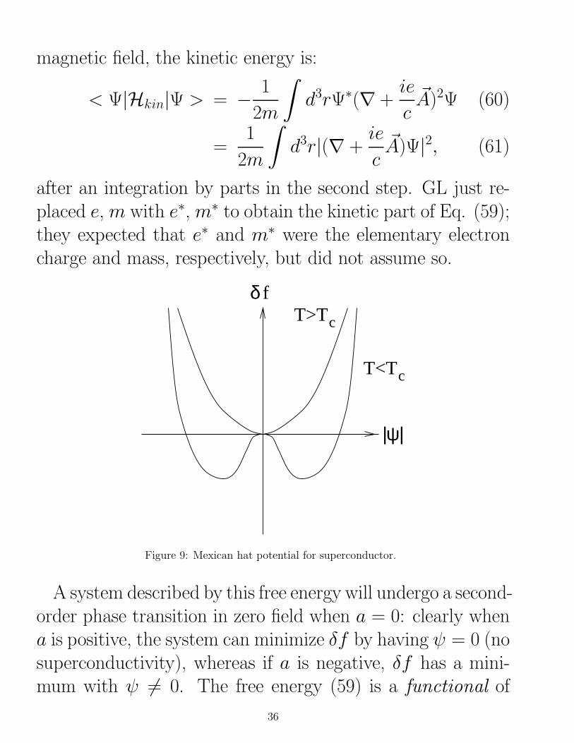
A system described by this free energy will undergo a second-order phase transition in zero field when a = 0: clearly whena is positive, the system can minimize δf by having ψ = 0 (nosuperconductivity), whereas if a is negative, δf has a mini-mum with ψ 6= 0. The free energy (59) is a functional of

36

the order parameter ψ, meaning the actual value of the orderparameter realized in equilibrium satisfies δf/δψ = 0.18 No-tice f is independent of the phase φ of the order parameter,ψ ≡ |ψ|eiφ, and so the ground state for a < 0 is equivalentto any state ψ related to it by multiplication by a pure phase.This is the U (1) gauge invariance of which we spoke earlier.This symmetry is broken when the system chooses one of theground states (phases) upon condensation (Fig 1.).

For a uniform system in zero field, the total free energyF =

∫d3rf is minimized when f is, so one find for the order

parameter at the minimum,

|ψ|eq = [−a2b ]1/2, a < 0 (62)

|ψ|eq = 0, a > 0. (63)

When a changes sign, a minimum with a nonzero value be-comes possible. For a second order transition as one lowers thetemperature, we assume that a and b are smooth functions ofT near Tc. Since we are only interested in the region near Tc,we take only the leading terms in the Taylor series expansionsin this region: a(T,H) = a0(T − Tc) and b = constant. Eqs.(62) and (63) take the form:

|ψ(T )|eq = [a0(Tc−T )2b ]1/2, T < Tc (64)

|ψ(T )|eq = 0, T > Tc. (65)18Thus you should not be perturbed by the fact that f apparently depends on ψ even for a > 0. The value of f

in equilibrium will be fn = f [ψ = 0].

37

Substituting back into Eqs.59, we find:

fs(T )− fn(T ) = −a204b(Tc − T )2, T < Tc (66)

fs(T )− fn(T ) = 0, T > Tc. (67)

The idea now is to calculate various observables, and de-termine the GL coefficients for a given system. Once theyare determined, the theory acquires predictive power due toits extreme simplicity. It should be noted that GL theory isapplied to many systems, but it is in classic superconductorsthat it is most accurate, since the critical region, where de-viations from mean field theory are large, is of order 10−4 orless. Near the transition it may be taken to be exact for allpractical purposes. This is not the case for the HTSC, wherethe size of the critical region has been claimed to be as muchas 10-20K in some samples.

Supercurrents. Let’s now focus our attention on theterm in the GL free energy which leads to supercurrents, thekinetic energy part:

Fkin =

∫

d3r1

2m∗|(∇ +ie∗

c~A)ψ|2 (68)

=

∫

d3r1

2m∗ [(∇|ψ|)2 + (∇φ− e∗/cA)2|ψ|2]. (69)

These expressions deserve several remarks. First, note thatthe free energy is gauge invariant, if we make the transforma-tion ~A→ ~A+∇Λ, where Λ is any scalar function of position,while at the same time changing ψ → ψ exp(−ie∗Λ/c) . Sec-ond, note that in the last step above I have split the kinetic

38

part of f into a term dependent on the gradients of the orderparameter magnitude |ψ| and on the gradients of the phaseφ. Let us use a little intuition to guess what these termsmean. The energy of the superconducting state below Tc islower than that of the normal state by an amount called thecondensation energy.19 From Eq. (59) in zero field this is oforder |ψ|2 very close to the transition. To make spatial vari-ations of the magnitude of ψ must cost a significant fractionof the condensation energy in the region of space in which itoccurs.20 On the other hand, the zero-field free energy is ac-tually invariant with respect to changes in φ, so fluctuationsof φ alone actually cost no energy.

With this in mind, let’s ask what will happen if we applya weak magnetic field described by A to the system. Sinceit is a small perturbation, we don’t expect it to couple to |ψ|but rather to the phase φ. The kinetic energy density shouldthen reduce to the second term in Eq. (69), and furthermorewe expect that it should reduce to the intuitive two-fluid ex-pression for the kinetic energy due to supercurrents, 1

2mnsv2s .

Recall from the superfluid He analogy, we expect |ψ|2 ≡ n∗sto be a kind of density of superconducting electrons, but thatwe aren’t certain of the charge or mass of the “particles”. Solet’s put

fkin '1

2m∗ |(∇+ie∗

c~A)ψ|2. =

∫

d3r1

2m∗(∇φ+e∗/cA)2|ψ|2 ≡ 1

2m∗n∗sv

2s .

(70)

Comparing the forms, we find that the superfluid velocity19We will see below from the Gorkov derivation of GL from BCS that it is of order N(0)∆2.20We can make an analogy with a ferromagnet, where if we have a domain wall the magnetization must go to zero

at the domain boundary, costing lots of surface energy.

39

must be

~vs =1

m∗(∇φ +e∗

c~A). (71)

Thus the gradient of the phase is related to the superfluidvelocity, but the vector potential also appears to keep theentire formalism gauge-invariant.

Meissner effect. The Meissner effect now follows imme-diately from the two-fluid identifications we have made. Thesupercurrent density will certainly be just

~js = −e∗n∗s~vs = −e∗n∗sm∗ (∇φ +

e∗

c~A). (72)

Taking the curl of this equation, the phase drops out, and wefind the magnetic field:

∇× ~js = −e∗2n∗sm∗c

~B. (73)

Now recall the Maxwell equation

~js =c

4π∇× ~B, (74)

which, when combined with (14), gives

c

4π∇×∇× ~B = − c

4π∇2 ~B = −e

∗2nsm∗c

~B, (75)

orλ2∇2 ~B = ~B, (76)

where

λ =m∗c2

4πe∗2n∗s

1/2

. (77)

40

Notice now that if we use what we know about Cooper pairs,this expression reduces to the BCS/London penetration depth.We assume e∗ is the charge of the pair, namely e∗ = 2e, andsimilarly m∗ = 2m, and |ψ|2 = n∗s = ns/2 since n∗s is thedensity of pairs.

Flux quantization. If we look at the flux quantizationdescribed in Part 1 of these notes, it is clear from our sub-sequent discussion of the Meissner effect, that the currentswhich lead to flux quantization will only flow in a small partof the cross section, a layer of thickness λ. This layer enclosesthe flux passing through the toroid. Draw a contour C in theinterior of the toroid, as shown in Figure 10. Then vs = 0everywhere on C. It follows that

js

C

λΦ

Figure 10: Quantization of flux in a toroid.

0 =

∮

C

d~ · ~vs =1

m∗

∮

C

d~ · (∇φ +e∗

c~A). (78)

The last integral may be evaluated using∮

C

d~ · ∇φ = 2π × integer, (79)

41

which follows from the requirement that ψ be single-valued asin quantum mechanics. Having n 6= 0 requires that one notbe able to shrink the contour to a point, i.e. that the samplehas a hole as in our superconducting ring. The line integralof the vector potential is and

e∗

c

∮

C

d~ · ~A =e∗

c

∫

S

d~S · ∇ × ~A (80)

=e∗

c

∫

S

d~S · ~B (81)

=e∗

cΦ. (82)

Here S is a surface spanning the hole and Φ the flux throughthe hole. Combining these results,

Φ = 2π~c

2en = n

hc

2e= nΦ0, (83)

where n is a integer, Φ0 is the flux quantum, and I’ve rein-serted the correct factor of ~ in the first step to make the unitsright. Flux quantization indeed follows from the fact that thecurrent is the result of a phase gradient.21

Derivation from Microscopic Theory. One of thereasons the GL theory did not enjoy much success at firstwas the fact that it is purely phenomenological, in the sensethat the parameters a0, b,m

∗ are not given within any micro-scopic framework. The BCS theory is such a framework, andgives values for these coefficients which set the scale for all

21It is important to note, however, that a phase gradient doesn’t guarantee that a current is flowing. For example,in the interior of the system depicted in Fig. 2, both ∇φ and ~A are nonzero in the most convenient gauge, and canceleach other!

42

quantities calculable from the GL free energy. The GL theoryis more general, however, since, e.g. for strong coupling su-perconductors the weak coupling values of the coefficients aresimply replaced by different ones of the same order of mag-nitude, without changing the form of the GL free energy. Inconsequence, the dependence of observables on temperature,field, etc, will obey the same universal forms.

The GL theory was derived from BCS by Gor’kov. Thecalculation is beyond the scope of this course, but can befound in many texts.

6.2 Type I and Type II superconductivity

Now let’s look at the problem of the instability of the normalstate to superconductivity in finite magnetic fieldH. At whatmagnetic field to we expect superconductivity to be destroyed,for a given T < Tc?

22 Well, overall energy is conserved, sothe total condensation energy of the system in zero field,fs−fn(T ) of the system must be equal to the magnetic field energy∫d3rH2/8π the system would have contained at the critical

fieldHc in the absence of the Meissner effect. For a completelyhomogeneous system I then have

fs(T )− fn(T ) = −H2c /8π, (84)

and from Eq. (8) this means that, near Tc,

Hc =

√

2πa20b

(Tc − T ). (85)

22Clearly it will destroy superconductivity since it breaks the degenerace of between the two componenets of aCooper pair.

43

Whether this thermodynamic critical field Hc actually rep-resents the applied field at which flux penetrates the sampledepends on geometry. We assumed in the simplified treat-ment above that the field at the sample surface was the sameas the applied field. Clearly for any realistic sample placedin a field, the lines of field will have to follow the contourof the sample if it excludes the field from its interior. Thismeans the value of H at different points on the surface willbe different: the homogeneity assumption we made will notquite hold. If we imagine ramping up the applied field fromzero, there will inevitably come a point Happl = Happl,c wherethe field at certain points on the sample surface exceeds thecritical field, but at other points does not. For applied fieldsHappl,c < Happl < Hc, part of the sample will then be normal,with local field penetration, and other parts will still excludefield and be superconducting. This is the intermediate state

of a type I superconductor. The structure of this state for areal sample is typically a complicated ”striped” pattern of su-perconducting and normal phases. Even for small fields, edgesand corners of samples typically go normal because the fieldlines bunch up there; these are called ”demagnetizing effects”,and must be accounted for in a quantitatively accurate mea-surement of, say, the penetration depth. It is important tonote that these patterns are completely geometry dependent,and have no intrinsic length scale associated with them.

In the 50’s, there were several materials known, however,in which the flux in sufficiently large fields penetrated the

44

sample in a manner which did not appear to be geometry de-pendent. For example, samples of these so-called ”type II”superconductors with nearly zero demagnetizing factors (longthin plates placed parallel to the field) also showed flux pen-etration in the superconducting state. The type-II materialsexhibit a second-order transition at finite field and the fluxB through the sample varies continuously in the supercon-ducting state. Therefore the mixed state must have currentsflowing, and yet the Meissner effect is not realized, so that theLondon equation somehow does not hold.

The answer was provided by Abrikosov in 1957 [A.A.A.,Sov. Phys. JETP 5, 1174 (1957).] in a paper which Landauapparently held up for several years because he did not be-lieve it. Let us neglect the effects of geometry again, and goback to our theorist’s sample with zero demagnetizing factor.Can we relax any of the assumptions that led to the Lon-don equation (72)? Only one is potentially problematic, thatn∗s(r) = |ψ(r)|2 = constant independent of position. Let’sexamine–as Abrikosov did–the energy cost of making spatialvariations of the order parameter. The free energy in zerofield is

F =

∫

d3r[a|ψ|2 + 1

2m∗|∇ψ|2 + b|ψ|4], (86)

or1

−aF =

∫

d3r[−|ψ|2 + ξ2|∇ψ|2 + b

−a|ψ|4], (87)

45

where I’ve put

ξ = [1

−2m∗a]1/2 = [

1

−2m∗a0(Tc − T )]1/2. (88)

Clearly the length ξ represents some kind of stiffness of thequantitiy |ψ|2, the superfluid density. [Check that it does in-deed have dimensions of length!] If ξ, the so-called coherence

length, is small, the energy cost of ns varying from place toplace will be small. If the order parameter is somehow changedfrom its homogeneous equilibrium value at one point in spaceby an external force, ξ specifies the length scale over whichit ”heals”. We can then investigate the possibility that, asthe kinetic energy of superfluid flow increases with increasingfield, if ξ is small enough it might eventually become favorableto ”bend” |ψ|2 instead. In typical type I materials, ξ(T = 0)is of order several hundreds or even thousands of Angstrom,but in heavy fermion superconductors, for example, coher-ence lengths are of order 50-100A. The smallest coherencelengths are attained in the HTSC, where ξab is of order 12-15A, whereas ξc is only 2-3A.

The general problem of minimizing F when ψ depends onposition is extremely difficult. However, we are mainly in-terested in the phase boundary where ψ is small, so life is abit simpler. Let’s recall our quantum mechanics analogy oncemore so as to write F in the form:

F =

∫

d3r[a|ψ|2 + b|ψ|4]+ < ψ|Hkin|ψ >, (89)

46

where Hkin is the operator

− 1

2m∗(∇ +ie∗

c~A)2. (90)

Now note 1) sufficiently close to the transition, we mayalways neglect the 4th-order term, which is much smaller;2) to minimize F , it suffices to minimize < Hkin >, sincethe |ψ|2 term will simply fix the overall normalization. Thevariational principle of quantum mechanics states that theminimum value of < H > over all possible ψ is achievedwhen ψ is the ground state (for a given normalization of ψ).So we need only solve the eigenvalue problem

Hkinψj = Ejψj (91)

for the lowest eigenvalue, Ej, and corresponding eigenfunction

ψj. For the given form of Hkin, this reduces to the classicquantum mechanics problem of a charged particle moving inan applied magnetic field. The applied field H is essentiallythe same as the microscopic field B since ψ is so small (at thephase boundary only!). I’ll remind you of the solution, due toto Landau, in order to fix notation. We choose a convenientgauge,

A = −Hyx, (92)

in which Eq. 44 becomes

1

2m∗ [(−i∂

∂x+

y

`2M)2 − ∂2

∂y2− ∂2

∂z2]ψj = Ejψj, (93)

where `M = (c/e∗H)1/2 is the magnetic length. Since the co-ordinates x and z don’t appear explicitly, we make the ansatz

47

of a plane wave along those directions:

ψ = η(y)eikxx+ikzz, (94)

yielding

1

2m∗ [(kx +y

`2M)2 − ∂2

∂y2+ k2z ]η(y) = Eη(y). (95)

But this you will recognize as just the equation for a one-dimensional harmonic oscillator centered at the point y =−kx`2M with an additional additive constant k2z/2m

∗ in theenergy. Recall the standard harmonic oscillator equation

(− 1

2m

∂2

∂x2+1

2kx2)Ψ = EΨ, (96)

with ground state energy

E0 =ω0

2=

1

2(k/m)1/2, (97)

where k is the spring constant, and ground state wavefunc-tion corresponding to the lowest order Hermite polynomial,

Ψ0 ≈ exp[−(mk/4)1/2x2]. (98)

Let’s just take over these results, identifying

Hkinψkx,kz =e∗H

2m∗cψkx,kz. (99)

The ground state eigenfunction may then be chosen as

ψkx,kz = ψ0(π`2ML2y

)−1/4eikxx+ikzz exp[−(y + kx`2M)2/2`2M)],

(100)

48

whereLy is the size of the sample in the y direction (LxLyLz =V = 1). The wave functions are normalized such that

∫

d3r|ψkx,kz|2 = ψ20 (101)

(since I set the volume of the system to 1). The prefactorsare chosen such that ψ2

0 represents the average superfluid den-stity. One important aspect of the particle in a field problemseen from the above solution is the large degeneracy of theground state: the energy is independent of the variable kx,for example, corresponding to many possible orbit centers.

We have now found the wavefunction which minimizes <Hkin >. Substituting back into (89), we find using (99)

F = [a0(T − Tc) +e∗H

2m∗c]

∫

d3r|ψ|2 + b

∫

d3r|ψ|4. (102)

When the coefficient of the quadratic term changes sign, wehave a transition. The field at which this occurs is called theupper critical field Hc2,

Hc2(T ) =2m∗ca0e∗

(Tc − T ). (103)

What is the criterion which distinguishes type-I and type IImaterials? Start in the normal state for T < Tc as shown inFigure 3, and reduce the field. Eventually one crosses eitherHc or Hc2 first. Whichever is crossed first determines thenature of the instability in finite field, i.e. whether the sampleexpels all the field, or allows flux (vortex) penetration (seesection C).

49

c1H

H

H

Meissner phase

T

H

Normal statec2

c

Figure 11: Phase boundaries for classic type II superconductor.

In the figure, I have displayed the situation where Hc2 ishigher, meaning it is encountered first. The criterion for thedividing line between type 1 and type II is simply

|dHc

dT| = |dHc2

dT| (104)

at Tc, or, using the results (85) and (103),

(m∗)2c2b

π(e∗)2=

1

2. (105)

This criterion is a bit difficult to extract information from inits current form. Let’s define the GL parameter κ to be theratio of the two fundamental lengths we have identified so far,the penetration depth and the coherence length:

κ =λ

ξ. (106)

Recalling that

λ2 = − m∗c2

4πe∗2n∗s= −m∗c2b

2πe∗2a(107)

50

and

ξ2 = − 1

2m∗a. (108)

The criterion (58) now becomes

κ2 =m∗c2b/2πe∗2a

1/2m∗a=

(m∗)2c2b

πe∗2=

1

2. (109)

Therefore a material is type I (II) if κ is less than (greaterthan) 1√

2. In type-I superconductors, the coherence length is

large compared to the penetration depth, and the system isstiff with respect to changes in the superfluid density. Thisgives rise to the Meissner effect, where ns is nearly constantover the screened part of the sample. Type-II systems can’tscreen out the field close to Hc2 since their stiffness is toosmall. The screening is incomplete, and the system must de-cide what pattern of spatial variation and flux penetration ismost favorable from an energetic point of view. The result isthe vortex lattice first described by Abrikosov.

6.3 Vortex Lattice

I commented above on the huge degeneracy of the wave func-tions (100). In particular, for fixed kz = 0, there are as manyground states as allowed values of the parameter kx. AtHc2 itdidn’t matter, since we could use the eigenvalue alone to de-termine the phase boundary. BelowHc2 the fourth order termbecomes important, and the minimization of f is no longer aneigenvalue problem. Let’s make the plausible assumption thatif some spatially varying order parameter structure is going

51

to form below Hc2, it will be periodic with period 2π/q, i.e.the system selects some wave vector q for energetic reasons.The x-dependence of the wave functions

ψkx,kz=0 = ψ0(π`2ML2y

)−1/4eikxx exp[−(y+kx`2M)2/2`2M)]. (110)

is given through plane wave phases, eikxx. If we choose kx =qnx, with nx =integer, all such functions will be invariantunder x → x + 2π/q. Not all nx’s are allowed, however: thecenter of the ”orbit”, kx`

2M should be inside the sample:

−Ly/2 < kx`2M = q`2Mnx < Ly/2, (111)

Thus nx is restricted such that

− Ly2q`2

= −nmax/2 < nx < nmax/2 =Ly2q`2

(112)

and the total number of degenerate functions is Ly/(q`2M).

Clearly we need to build up a periodic spatially varyingstructure out of wave functions of this type, with ”centers”distributed somehow. What is the criterion which determinesthis structure? All the wave functions (110) minimize <Hkin >, and are normalized to

∫d3r|ψ|2 = |ψ0|2. They are

all therefore degenerate at the level of the quadratic GL freeenergy, F =

∫d3r|ψ|2+ < Hkin >. The fourth order term

must stabilize some linear combination of them. We thereforewrite

ψ(r) =∑

nx

Cnxψnx(r), (113)

52

with the normalization∑

nx|Cnx|2 = 1, which enforces

∫d3r|ψ(r)|2 =

ψ20. Note this must minimize < Hkin >. Let’s therefore

choose the Cnx and q to minimize the remaining terms in F ,∫d3r[a|ψ|2+b|ψ|4]. Substituting and using the normalization

condition and orthogonality of the different ψkz,kx, we find

f = aψ20 + bψ4

0. (114)

with

a(H, T ) = a0(T − Tc) +e∗H

2m∗c=

e∗

2m∗c(H −Hc2(T )), (115)

b(H) = sb, (116)

and

s = (π`2ML2y

)−1nmax∑

nx1,nx2,nx3,nx4

C∗nx1C∗nx2Cnx3Cnx4

∫

dz

∫

dx eiq(−nx1−nx2+nx3+nx4)x ×∫

dy e− 1

2`2M

[(y+qnx1`2M )2+(y+qnx2`

2M )2+(y+qnx3`

2M )2+(y+qnx4`

2M )2]

.(117)

The form of f [ψ0] is now the same as in zero field, so weimmediately find that in equilibrium,

ψ0|eq = (−a2b

)1/2. (118)

and

f =−a24b

. (119)

This expression depends on the variational parameters Cnx, qonly through the quantity s appearing in b. Thus if we mini-mize s, we will minimize f (remember b > 0, so f < 0). The

53

minimization of the complicated expression (117) with con-straint

∑

nx|Cnx|2 = 1 is difficult enough that A. Abrikosov

made a mistake the first time he did it, and I won’t inflict thefull solution on you. To get an idea what it might look like,however, let’s look at a very symmetric linear combination,one where all the Cnx’s are equal:

Cn = n−1/2max . (120)

Then

ψ(r) ∼∑

n

einqx exp[−(y + nq`2M)2/2`2M ], (121)

which is periodic in x with period 2π/q,

ψ(x + 2π/q, y) = ψ(x, y), (122)

and periodic in y with period q`2M , up to a phase factor

ψ(x, y + q`2M) = e−iqxψ(x, y). (123)

in a sufficiently large system. Note if q =√2π/`M , |ψ|2 forms

a square lattice! The area of a unit cell is (2π/q)× (q`2M) =2π`2M , and the flux through each one is therefore

Φcell = 2π`2MH = 2πc

e∗HH =

hc

2e= Φ0 (124)

where I inserted a factor of ~ in the last step. We haven’tperformed the minimization explicitly, but this is a charac-teristic of the solution, that each cell contains just one fluxquantum. The picture is crudely depicted in Fig. 12a). Noteby symmetry that the currents must cancel on the boundaries

54

s=1.18 s=1.16

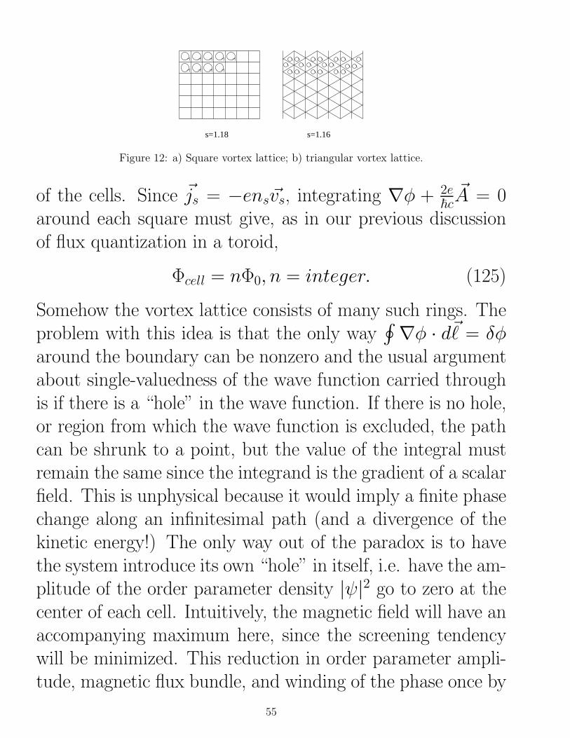
Figure 12: a) Square vortex lattice; b) triangular vortex lattice.

of the cells. Since ~js = −ens~vs, integrating ∇φ + 2e~c~A = 0

around each square must give, as in our previous discussionof flux quantization in a toroid,

Φcell = nΦ0, n = integer. (125)

Somehow the vortex lattice consists of many such rings. Theproblem with this idea is that the only way

∮∇φ · d~ = δφ

around the boundary can be nonzero and the usual argumentabout single-valuedness of the wave function carried throughis if there is a “hole” in the wave function. If there is no hole,or region from which the wave function is excluded, the pathcan be shrunk to a point, but the value of the integral mustremain the same since the integrand is the gradient of a scalarfield. This is unphysical because it would imply a finite phasechange along an infinitesimal path (and a divergence of thekinetic energy!) The only way out of the paradox is to havethe system introduce its own “hole” in itself, i.e. have the am-plitude of the order parameter density |ψ|2 go to zero at thecenter of each cell. Intuitively, the magnetic field will have anaccompanying maximum here, since the screening tendencywill be minimized. This reduction in order parameter ampli-tude, magnetic flux bundle, and winding of the phase once by

55

2π constitute a magnetic “vortex”, which I’ll discuss in moredetail next time.

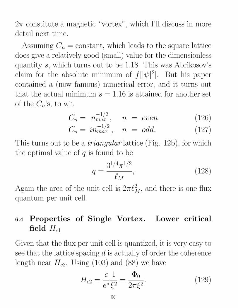
Assuming Cn = constant, which leads to the square latticedoes give a relatively good (small) value for the dimensionlessquantity s, which turns out to be 1.18. This was Abrikosov’sclaim for the absolute minimum of f [|ψ|2]. But his papercontained a (now famous) numerical error, and it turns outthat the actual minimum s = 1.16 is attained for another setof the Cn’s, to wit

Cn = n−1/2max , n = even (126)

Cn = in−1/2max , n = odd. (127)

This turns out to be a triangular lattice (Fig. 12b), for whichthe optimal value of q is found to be

q =31/4π1/2

`M, (128)

Again the area of the unit cell is 2π`2M , and there is one fluxquantum per unit cell.

6.4 Properties of Single Vortex. Lower critical

field Hc1

Given that the flux per unit cell is quantized, it is very easy tosee that the lattice spacing d is actually of order the coherencelength near Hc2. Using (103) and (88) we have

Hc2 =c

e∗1

ξ2=

Φ0

2πξ2. (129)

56

On the other hand, as H is reduced, d must increase. To seethis, note that the area of the triangular lattice unit cell isA =

√3d2/2, and that there is one quantum of flux per cell,

A = Φ0/H . Then the lattice constant may be expressed as

d =4π√3ξ(Hc2

H)1/2. (130)

Since λ ξ is the length scale on which supercurrents andmagnetic fields vary, we expect the size of a magnetic vor-tex to be about λ. This means at Hc2 vortices are stronglyoverlapping, but as the field is lowered, the vortices separate,according to (124), and may eventually be shown to influenceeach other only weakly. To find the structure of an isolatedvortex is a straightforward but tedious exercise in minimizingthe GL free energy, and in fact can only be done numericallyin full detail. But let’s exploit the fact that we are inter-ested primarily in strongly type-II systems, and therefore goback to the London equation we solved to find the penetrationdepth in the half-space geometry for weak fields, allow ns tovary spatially, and look for vortex-like solutions. For example,equation (75) may be written

−λ2∇×∇× ~B = ~B. (131)

Let’s integrate this equation over a surface perpendicular tothe field ~B = ~B(x, y)z spanning one cell of the vortex lattice:

−λ2∫

∇× (∇× ~B) · d~S =

∫

~B · d~S, (132)

−λ24πc

∮

~js · d~ = Φ0. (133)

57

But we have already argued that ~js · d~ should be zero onthe boundary of a cell, so the left side is zero and there isa contradiction. What is wrong? The equation came fromassuming a two-fluid hydrodynamics for the superconductor,with a nonzero ns everywhere. We derived it, in fact, fromBCS theory, but only for the case where ns was constant.Clearly there must be another term in the equation when avortex-type solution is present, one which can only contributeover the region where the superfluid density is strongly varyingin space, i.e. the coherence length-sized region in the middleof the vortex where the order parameter goes to zero (vortex“core”). Let’s simply add a term which enables us to getthe right amount of flux to Eq. (131). In general we shouldprobably assume something like

λ2∇×∇× ~B + ~B = Φ0g(~r)z (134)

where g(r) is some function which is only nonzero in the core.The flux will then come out right if we demand

∫d3rg(~r) =

1. But let’s simplify things even further, by using the factthat ξ λ: let’s treat the core as having negligible size,which means it is just a line singularity. We therefore putg(~r) = δ(~r). Then the modified London equation with linesingularity acting as an inhomogeneous “source term” reads

−λ2∇2 ~B + ~B = Φ0δ2(~r)z (135)

−λ21ρ

∂

∂ρ(ρ∂Bz

∂ρ) +Bz = Φ0δ

2(~r), (136)

58

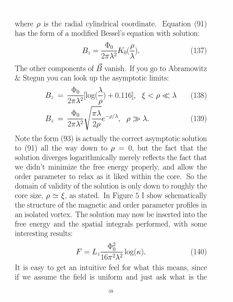
where ρ is the radial cylindrical coordinate. Equation (91)has the form of a modified Bessel’s equation with solution:

Bz =Φ0

2πλ2K0(

ρ

λ). (137)

The other components of ~B vanish. If you go to Abramowitz& Stegun you can look up the asymptotic limits:

Bz =Φ0

2πλ2[log(

λ

ρ) + 0.116], ξ < ρ λ (138)

Bz =Φ0

2πλ2

√

πλ

2ρe−ρ/λ, ρ λ. (139)

Note the form (93) is actually the correct asymptotic solutionto (91) all the way down to ρ = 0, but the fact that thesolution diverges logarithmically merely reflects the fact thatwe didn’t minimize the free energy properly, and allow theorder parameter to relax as it liked within the core. So thedomain of validity of the solution is only down to roughly thecore size, ρ ' ξ, as stated. In Figure 5 I show schematicallythe structure of the magnetic and order parameter profiles inan isolated vortex. The solution may now be inserted into thefree energy and the spatial integrals performed, with someinteresting results:

F = LzΦ20

16π2λ2log(κ). (140)

It is easy to get an intuitive feel for what this means, sinceif we assume the field is uniform and just ask what is the

59

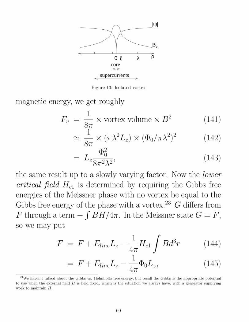
core

ρλξ0

supercurrents

|ψ|

Bz

Figure 13: Isolated vortex

magnetic energy, we get roughly

Fv =1

8π× vortex volume×B2 (141)

' 1

8π× (πλ2Lz)× (Φ0/πλ

2)2 (142)

= LzΦ20

8π2λ2, (143)

the same result up to a slowly varying factor. Now the lowercritical field Hc1 is determined by requiring the Gibbs freeenergies of the Meissner phase with no vortex be equal to theGibbs free energy of the phase with a vortex.23 G differs fromF through a term −

∫BH/4π. In the Meissner state G = F ,

so we may put

F = F + ElineLz −1

4πHc1

∫

Bd3r (144)

= F + ElineLz −1

4πΦ0Lz, (145)

23We haven’t talked about the Gibbs vs. Helmholtz free energy, but recall the Gibbs is the appropriate potentialto use when the external field H is held fixed, which is the situation we always have, with a generator supplyingwork to maintain H .

60

where Eline is the free energy per unit length of the vortexitself. Therefore

Hc1 =4πEline

Φ0(146)

is the upper critical field. But the line energy is given precisely

by Eq. (95), Eline =Φ20

16π2λ2log(κ), so

Hc1(T ) =Φ0

4πλ2log(κ). (147)

6.5 Josephson Effect

In 1962 Brian Josephson24, then a 22–year old graduate stu-dent, made a remarkable prediction that two superconductorsseparated by a thin insulating barrier should give rise to aspontaneous (zero voltage) DC current, Is = Ic sin∆φ, where∆φ is the difference in phase across the junction. And thatif a finite (DC) voltage were applied, an AC current with fre-quency ω = 2eV/~ would flow. Ic is called the Josephsoncritical current.There is a myth that Brian Josephson did his calculation

(1962) and won the Nobel prize (1973) as part of the solu-tion to a homework problem of Phil Anderson’s. The truthis that Anderson was a lecturer on sabbatical at Cambridgein 1961-62, and he gave a series of lectures in which he men-tioned the problem of tunneling between two superconductors,which Josephson then promptly solved. The idea was opposedat first by John Bardeen, who felt that pairing could not exist

24Phys. Lett. 1, 251 (1962)

61

in the barrier region25. Thus much of the early debate cen-tered on the nature of the tunneling process, whereas in facttoday we know that the Josephson effect occurs in a variety ofsituations whenever two superconductors are separated by a“weak link”, which can be an insulating region, normal metal,or short, narrow constriction.26

Let’s first consider the last example as the conceptually sim-plest. The Ginzburg–Landau equation appropriate for thissituation may be written

ξ2d2f

dx2+ f − f 3 = 0 (148)

where ξ =√

~

2m∗a(T ) is the GL coherence length and f(x) ≡Ψ(x)/Ψ∞. Take L ξ, so the deviations of Ψ coming fromthe bulk value Ψ1 of the first SC is small, and vice versa forthe second SC. Changes of Ψ in the constriction occur overa length scale of L, so that the first term is of O((ξ/L)2) f − f 3. So we must solve a Laplace equation for f , (d

2fdx2

= 0)25Physics Today, July 200126In Je. 2009 I received an email from Brian Josephson correcting this version of the history:

Date: Wed, 10 Jun 2009 09:43:54 +0100

From: Brian Josephson <bdj10@cam.ac.uk>

To: pjh@phys.ufl.edu

Subject: the Josephson myth

Dear Peter,

While browsing I came across your mention of the ’myth’ that I discovered the effect because

of a problem set by Anderson. Your correction is not completely correct either! It was

Pippard, my supervisor, who drew my attention to Giaevar’s tunnelling expts. and his theory,

which started me thinking (especially as to how one could get away without using coherence

factors). Anderson on the other hand told me of the Cohen/Falicov/Phillps calculation involving

a single superconductor when it came our in PRL, which gave me the idea of how to do the two-sc.

case. Previously I had got the broken symmetry idea which was crucial from a number of papers

including Anderson’s pseudospin model, and also expounded in his lecture course which I went to.

Best regards, Brian J.

62

with B.C. f(0) = 1, f(L) = ei∆Φ. The solution will be

f =

(

1− x

L

)

+x

Lei∆φ. (149)

The solution can be thought of as two terms, the first Ψ1,beginning to “leak” into the constriction from the left, thesecond Ψ2 leaking into the constriction from the right. TheGL expression for the current will be

j =e∗~

2m∗i

(Ψ∗∇Ψ− Ψ∇Ψ∗)− e∗2

m∗cΨ∗ΨA

︸ ︷︷ ︸zero

=e∗~

2m∗iΨ2

∞

[(

1− x

L+x

Le−i∆φ

)(

− 1

L+

1

Lei∆φ

)

− c.c

]

=e∗~Ψ2

∞m∗L

sin∆φ, (150)

which means that the current will be

I = Ic sin∆φ, (151)

Ic =e∗~Ψ2

∞m∗L

A, (152)

where A is the cross–section.Given that we have two weakly coupled QM systems, it is

“not unreasonable” (justified by microscopic theory) to writedown coupled Schrodinger equations

i∂Ψ1

∂t= E1Ψ1 + αΨ2 (153)

i∂Ψ2

∂t= E2Ψ2 + αΨ1 (154)

63

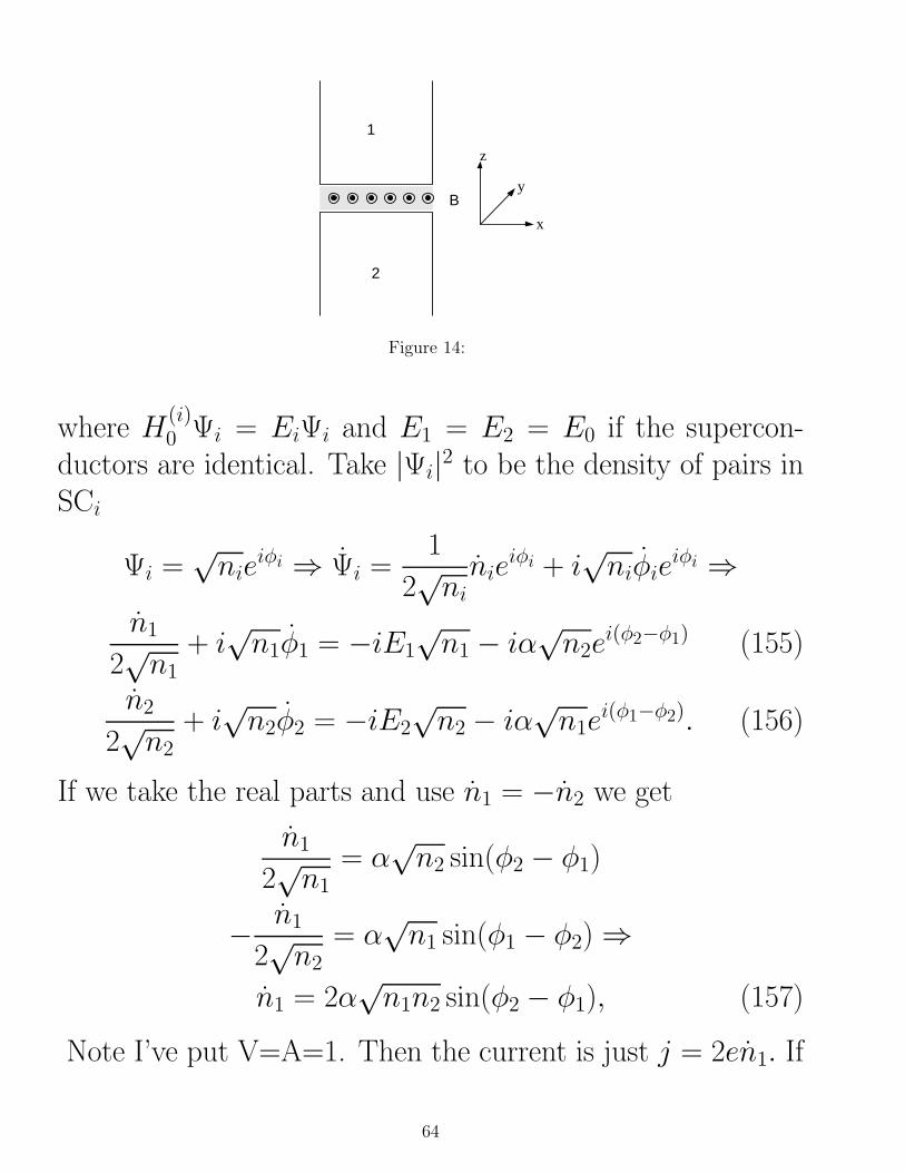
1

2

Βx

y

z

Figure 14:

where H(i)0 Ψi = EiΨi and E1 = E2 = E0 if the supercon-

ductors are identical. Take |Ψi|2 to be the density of pairs inSCi

Ψi =√nie

iφi ⇒ Ψi =1

2√ninie

iφi + i√niφie

iφi ⇒n1

2√n1

+ i√n1φ1 = −iE1

√n1 − iα

√n2e

i(φ2−φ1) (155)

n22√n2

+ i√n2φ2 = −iE2

√n2 − iα

√n1e

i(φ1−φ2). (156)

If we take the real parts and use n1 = −n2 we getn1

2√n1

= α√n2 sin(φ2 − φ1)

− n12√n2

= α√n1 sin(φ1 − φ2) ⇒

n1 = 2α√n1n2 sin(φ2 − φ1), (157)

Note I’ve put V=A=1. Then the current is just j = 2en1. If

64

we take the imaginary parts we have√n1φ1 = −E1

√n1 − α

√n2 cos(φ2 − φ1) (158)

√n2φ2 = −E2

√n2 − α

√n1 cos(φ1 − φ2), (159)

and by subtracting and assuming n1 ' n2 (let’s couple 2identical superconductors at first) we get

φ1 − φ2 = E2 − E1 = 2e(V1 − V2) (160)

where for the second equality we used the fact that the po-tential difference between the superconductors shifts the pairenergies by −2eV . So we see that a finite voltage differenceleads to a time changing phase difference ∆φ which means anAC current via Eq. (157).Magnetic fields. Now put a flux through the junction where

the B field is along the −y direction and A = −Bxz. Thephase of the wave function Ψ must change by

φ→ φ− 2e

c

∫

dS ·A (161)

for the theory to be gauge invariant. Notice that φ is nowspace–dependent. So the Josephson equations will read

j = 4eα√n1n2

︸ ︷︷ ︸jc

sin

(

∆φ− 2e

c

∫ 2

1

dS ·A)

, (162)

2e(V1 − V2) =∂

∂t

(

φ2 − φ1 −2e

c

∫ 2

1

dS ·A)

, (163)

and since∫ 2

1

S ·A =

∫ d

0

dz(−Bx) = −Bxd, (164)

65

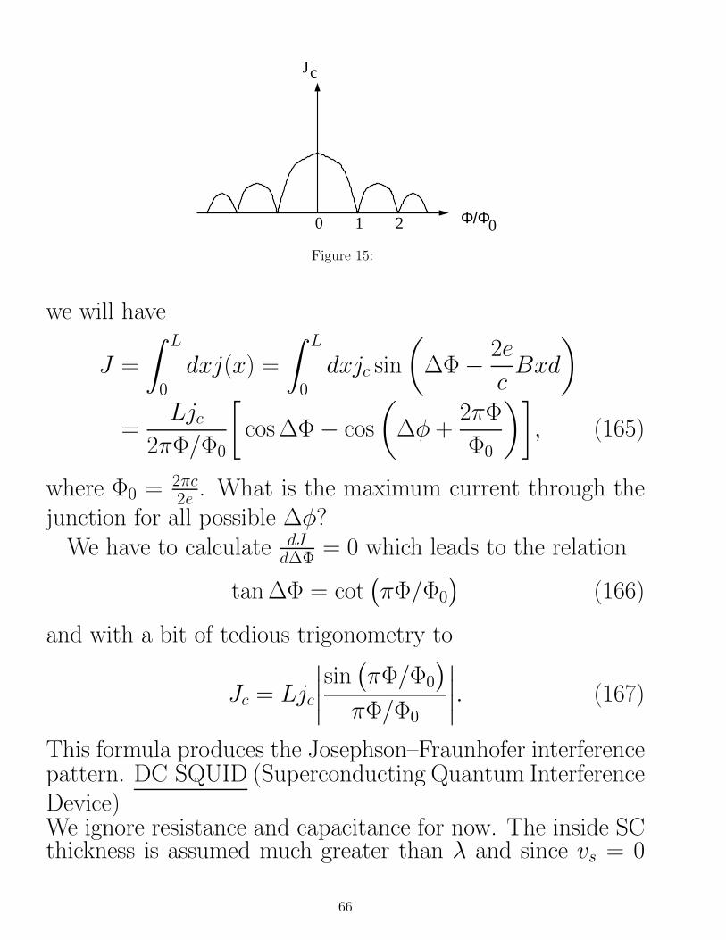
Φ/Φ

J

0 1 2 0

c

Figure 15:

we will have

J =

∫ L

0

dxj(x) =

∫ L

0

dxjc sin

(

∆Φ− 2e

cBxd

)

=Ljc

2πΦ/Φ0

[

cos∆Φ− cos

(

∆φ +2πΦ

Φ0

)]

, (165)

where Φ0 =2πc2e . What is the maximum current through the

junction for all possible ∆φ?We have to calculate dJ

d∆Φ = 0 which leads to the relation

tan∆Φ = cot(πΦ/Φ0

)(166)

and with a bit of tedious trigonometry to

Jc = Ljc

∣∣∣∣

sin(πΦ/Φ0

)

πΦ/Φ0

∣∣∣∣. (167)

This formula produces the Josephson–Fraunhofer interferencepattern. DC SQUID (Superconducting Quantum InterferenceDevice)We ignore resistance and capacitance for now. The inside SCthickness is assumed much greater than λ and since vs = 0

66

1 2

34

J JΦ

Figure 16:

we have ∇φ = 2A/Φ0. The flux will be

Φ =

∮

ds ·A =

∫ 2

1

ds · A+Φ0

2

∫ 3

2

ds · ∇φ+

∫ 4

3

ds ·A+Φ0

2

∫ 1

4

ds · ∇φ

=Φ0

2(φ3 − φ2) +

Φ0

2(φ1 − φ4) +

∫ 2

1

ds ·A+

∫ 4

3

ds ·A

=Φ0

2(φ1 − φ2) +

∫ 2

1

ds ·A︸ ︷︷ ︸

≡−γ12

+Φ0

2(φ3 − φ4) +

∫ 4

3

ds ·A︸ ︷︷ ︸

≡−γ34

Φ = γ43 − γ12. (168)

The Josephson current through the SQUID will be

J = Jc(sin γ12 + sin γ43

)

= Jc(sin γ12 + sin(γ12 + Φ)

). (169)

Which means that the current oscillates with the flux. Andas a result of that the SQUID can be a sensitive measure ofmagnetic fields. In practice we include the capacitance andresistance of the device.

67