Gini Covariance Matrix and its A ne Equivariant Version

Gini Covariance Matrix and its AffineEquivariant Version

October 25, 2016

Xin Dang1,3, Hailin Sang1 and Lauren Weatherall2

1Department of Mathematics, University of Mississippi, University, MS 38677,USA. E-mail addresses: [email protected], [email protected]

2 BlueCross & BlueShield of Mississippi, 3545 Lakeland Drive, Flowood, MS39232, USA. E-mail address: [email protected]

Abbreviated Title: Gini Covariance Matrix

Abstract

We propose a new covariance matrix called Gini covariance matrix (GCM),which is a natural generalization of univariate Gini mean difference (GMD) tothe multivariate case. The extension is based on the covariance representation ofGMD by applying the multivariate spatial rank function. We study properties ofGCM, especially in the elliptical distribution family. In order to gain the affineequivariance property for GCM, we utilize the transformation-retransformation(TR) technique and obtain an affine equivariant version GCM that turns out tobe a symmetrized M-functional. The influence function of those two GCM’s areobtained and their estimation has been presented. Asymptotic results of esti-mators have been established. A closely related scatter Kotz functional and itsestimator are also explored. Finally, asymptotical efficiency and finite sampleefficiency of the TR version GCM are compared with those of sample covari-ance matrix, Tyler-M estimator and other scatter estimators under differentdistributions.

Key words and phrases: Affine equivariance; efficiency; Gini mean difference;influence function; scatter M-estimator; spatial rank; symmetrization.

MSC 2010 subject classification: 62H10, 62H12

1 Introduction

Gini mean difference (GMD) was introduced by Corrado Gini in 1914 as analternative measure of variability. Since then, GMD and its derivatives suchas Gini index have been widely used in a variety of research fields especially in

3Corresponding author

1

finance, economics and social welfare (Yitzhaki and Schechtman, 2013). Ratherthan the assumption on the finite second moment, the GMD only requires ex-istence of the finite mean of the distribution (Yitzhaki, 2003). Hence GMD ismore robust than the variance and it is often used for heavy-tailed asymmetricdistributions, although it is less robust than some scale measures without anymoment conditions. On the other hand, GMD is highly efficient. The relativeefficiencies (RE) of the sample GMD with respect to sample standard deviationare about 0.98 under the normal distributions, 1.21 under the Laplace distribu-tion and 1.86 under the t(5) distribution (Nair, 1936; Gerstenberger and Vogel,2015). With a little loss on efficiency, GMD gains robustness against departuresfrom normal distributions.

In this paper, we extend GMD to the multivariate case. We propose theGini covariance matrix (GCM) as (2 times) the covariance of X with its spatialrank r(X), which is a direct generalization from a covariance representation ofthe univariate GMD. While the covariance matrix (Cov) is the covariance of Xwith itself and the rank covariance matrix (RCM) (Visuri et al., 2000) is thecovariance of r(X) with r(X), intuitively GCM is a new scatter measure be-tween Cov and RCM. With no surprise, the efficiency and robustness of sampleGCM are between those of sample Cov and RCM. In terms of balance betweenefficiency and robustness, sample Gini covariance matrix provides us an extramethod for multivariate statistical inference including multivariate analysis ofvariance, principle component analysis, factor analysis, and canonical correla-tion analysis.

As any estimator based on spatial signs and ranks, GCM is only orthogo-nally equivariant. In order to gain fully affine equivariant property, we utilizea transformation-retransformation (TR) technique (Charkraborty and Chaud-huri, 1996; Serfling, 2010) to obtain an affine equivariant version of GCM. Thewell-known scatter Tyler M-functional (Tyler, 1987) is a TR version of the spa-tial sign covariance matrix. Dumbgen (1998) considered symmetrized TR spatialsign covariance matrix on the difference of two independent vectors X1 −X2.Dumbgen et al. (2015) provided a general treatment on M-functionals of scatterbased on symmetrizations of arbitrary order. Our TR Gini covariance matrixturns out to be a pairwise symmetrized scatter M-functional. Compared to theregular M-functional, the symmetrized one has several advantages as emphasizedin Sirkia et al. (2007). The distribution of pairwise differences is symmetric at 0,hence avoids imposing some arbitrary definition of location for non-symmetricdistributions. For elliptical distributions, there is no need to estimate locationsimultaneously for scatter M-estimators. Hence they avoid restrictive regularityconditions for joint existence of location and scatter estimators and may takefewer iterations to converge than their counterparts. Further, a symmetrizedscatter matrix has the so-called block independence property: it is a block di-agonal matrix if the block components of the random vector are independent.Such a property holds naturally for the regular covariance matrix but may notfor general M-functionals and some robust alternatives (Nordhausen and Tyler,2015). Both versions of GCM have the block independence property and hencecan be applied to independent component analysis (Hyvarinen et al., 2001) or

2

invariant coordinate selection (Tyler et al., 2009). The price to pay for thoseadvantages of the pairwise difference approach is an increase of computationburden and a loss of some robustness. If a procedure has computation com-plexity O(n), its symmetrized one may require O(n2), although Dumbgen et al.(2016) have presented new algorithms for symmetrized M-estimators to reducethe computation time substantially. For large n, they approximate symmetrizedestimators by considering the surrogate ones rather than all pairwise differences.Their algorithms can easily be adopted for our estimators. The decrease of ro-bustness in symmetrized procedures seems to be understandable since one singleoutlier affects n − 1 pairwise differences. One must take into consideration ofefficiency, robustness and computation when choosing a proper procedure forapplications at hand.

Koshevoy et al. (2003) considered other multivariate extensions of meandeviation and Gini mean difference using the geometric volumes of zonotopesand lift-zonotopes. Their covariance matrices share many similar properties asour proposed ones, but ours enjoy simplicity and computational ease. Althoughthe approach differs from ours, it is worthwhile to mention that Serfling and Xiao(2007) also generalize GMD to multivariate case through L-moment approach.

The remainder of the paper is organized as follows. In Section 2, we firstreview the Gini mean difference and the spatial rank function, then introducethe Gini covariance matrix and its affine equivariant version. Section 3 exploresthe influence functions of the two Gini covariance matrices. Section 4 presentsestimation of the two Gini covariance matrices and asymptotical properties ofthe estimators. Asymptotic and finite sample efficiencies of the proposed TRGini covariance estimator have been studied and compared with other estima-tors. The paper ends with some final comments in Section 5. All proofs arereserved to Appendix Section.

2 Two Gini Covariance Matrices

2.1 Gini Mean Difference

Gini mean difference (GMD) was introduced as an alternative measure of vari-ability to the usual standard deviation. For a random variable X from a uni-variate distribution F , the GMD of X (or F ) is

σg = σg(X) = σg(F ) = E|X1 −X2|, (1)

where X1 and X2 are independent random variables from F . In contrast, thevariance of X (or F ) is

σ2v(F ) = var(X) =

1

2E(X1 −X2)2.

Rather than the assumption of finite second moment, the GMD only requiresexistence of a finite mean of F . Hence the Gini mean difference is often used for

3

heavy-tailed asymmetric distributions, especially in social welfare and the fieldsof decision-making under financial risk.

Among many representations such as Lorenz curve or L-functional formula-tions (Yitzhaki and Schechtman, 2013), we are interested in covariance formu-lations. One of them is

σg(F ) = 4Cov(X,F (X)).

While the variance is the covariance of X with itself, the GMD is (4 times)the covariance of X with F (X). In this spirit, two Gini-type alternatives tothe usual covariance for measuring the dependence of random variable X andanother random variable Y with distribution function H are

Covg(X,Y ) = 4Cov(X,H(Y )), Covg(Y,X) = 4Cov(Y, F (X)).

Such extensions are natural and useful (Yitzhaki, 2003; Carcea and Serfling,2015). However, a major drawback is the asymmetry between X and Y , i.e.,Covg(X,Y ) 6= Covg(Y,X), in general. An even worse part is that Covg(X,Y )and Covg(X,Y ) may have different signs in some cases (Yitzhaki, 2003), whichbrings substantial difficulty in interpretation. The asymmetry stems from theusage of F (X) or H(Y ), which can be thought as a standardized marginal rank.A symmetry one calls for a ‘joint’ rank of X and Y .

The other covariance type formulation for GMD is

σg(F ) = 2Cov(X, 2F (X)− 1),

allowing an insightful interpretation: σg(X) is twice of the covariance of Xand the centered rank function r(X) = 2F (X) − 1. r(X) is centered becauseEr(X) = 0 if F is continuous. So

σg(F ) = 2Cov(X, r(X)) = 2E(Xr(X)). (2)

A nice generalization of the centered rank in high dimensions provides a jointrank, and along with the representation of GMD in (2) yields a natural extensionof GMD for a multivariate distribution F .

2.2 Spatial Rank Function

Let X be a d-variate random vector from a continuous distribution F witha finite first moment and the expected Euclidean distance from x to X beD(x, F ) = EF ‖x − X‖. Then the gradient of D is denoted as the centeredspatial rank function (Mottonen et al., 1997), that is,

r(x) = ∇xD(x, F ) = Ex−X‖x−X‖

= E{s(x−X)}, (3)

where s(x) = x/‖x‖ (s(0) = 0) is the spatial sign function in Rd. The spatialrank function is the expected direction fromX to x. We call it centered because a

4

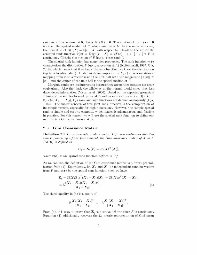
random rank is centered at 0, that is, Er(X) = 0. The solution of x in r(x) = 0is called the spatial median of F , which minimizes D. In the univariate case,the derivative of D(x, F ) = E|x −X| with respect to x leads to the univariatecentered rank function r(x) = Esign(x − X) = 2F (x) − 1 ∈ [−1, 1] if F iscontinuous. Clearly, the median of F has a center rank 0.

The spatial rank function has many nice properties. The rank function r(x)characterizes the distribution F (up to a location shift) (Koltchinskii, 1997; Oja,2010), which means that if we know the rank function, we know the distribution(up to a location shift). Under weak assumptions on F , r(x) is a one-to-onemapping from x to a vector inside the unit ball with the magnitude ‖r(x)‖ ∈[0, 1] and the center of the unit ball is the spatial median of F .

Marginal ranks are less interesting because they are neither rotation nor scaleequivariant. Also they lack the efficiency at the normal model since they lossdependence information (Visuri et al., 2000). Based on the expected geometricvolume of the simplex formed by x and d random vectors from F , i.e, D(x, F ) =EFV (x,X1, ...,Xd), Oja rank and sign functions are defined analogously (Oja,1983). The major concern of this joint rank function is the computation ofits sample version, especially for high dimensions. However, the sample spatialrank is simple and easy to compute, which makes it advantageous and feasiblein practice. For this reason, we will use the spatial rank function to define ourmultivariate Gini covariance matrix.

2.3 Gini Covariance Matrix

Definition 2.1 For a d-variate random vector X from a continuous distribu-tion F possessing a finite first moment, the Gini covariance matrix of X or F(GCM) is defined as

Σg = Σg(F ) = 2E[XrT (X)],

where r(x) is the spatial rank function defined in (3).

As we can see, the definition of the Gini covariance matrix is a direct general-ization from (2). Equivalently, let X1 and X2 be independent random vectorsfrom F and s(x) be the spatial sign function, then we have

Σg = 2EX1E[sT (X1 −X2)|X1] = 2E[X1sT (X1 −X2)]

= E(X1 −X2)(X1 −X2)T

‖X1 −X2‖. (4)

The third equality in (4) is a result of

EX1(X1 −X2)T

‖X1 −X2‖= −EX2(X1 −X2)T

‖X1 −X2‖.

From (4), it is easy to prove that Σg is positive definite since F is continuous.Equation (4) additionally recovers the L1 metric representation of Gini mean

5

difference (1) when d = 1. It also demonstrates that it is a pairwise differenceapproach defined without reference to a location parameter.

From (4), we can also write Σg as E(X1 −X2)sT (X1 −X2), which is theexpected matrix of the product of a pairwise difference and its directional signfunction. If we only use directional information of F , we obtain

Es(X1 −X2)sT (X1 −X2) = E(X1 −X2)(X1 −X2)T

‖X1 −X2‖2.

The resulting matrix is known as the symmetrized spatial sign covariance matrix(SSCM), which has been studied by Visuri et al. (2000), Croux et al. (2002)and Taskinen et al. (2012).

The spatial rank covariance matrix (RCM) is defined as the covariance ma-trix of spatial rank. That is,

Er(X)rT (X) = Es(X1 −X2)sT (X1 −X3) = E(X1 −X2)(X1 −X3)T

‖X1 −X2‖‖X1 −X3‖.

(5)

RCM and its modified version have been studied by Visuri et al. (2000) andYu et al. (2015). Since RCM uses three independent random vectors in itsdefinition, the sample RCM is more efficient than the sample SSCM.

Before we explore properties of the Gini covariance matrix, it is worthwhileto note that another useful extension of GMD from the covariance representationbased on the spatial rank function is 2EXTr(X). This generalization coincideswith the multivariate Gini mean difference defined in Koshevoy and Mosler(1997). That is, 2EXTr(X) = E‖X1 −X2‖. Clearly, it is also an immediateextension from the L1 metric representation of (1).

2.4 Properties of Gini covariance matrix

We study properties of the Gini covariance matrix under elliptical distributions.

Definition 2.2 A d-variate absolutely continuous random vector X has an el-liptical distribution if its density function is of the form

f(x|µ,Σ) = |Σ|−1/2g{(x− µ)TΣ−1(x− µ)}, (6)

for some positive definite symmetric matrix Σ and nonnegative function g with∫∞0td/2−1g(t)dt <∞.

If t(d−k)/2−1g(t) is integrable, then the kth moment of X exits. The parameterµ is the symmetric center and it equals the first moment if it exists. Thescatter parameter Σ is proportional to the covariance matrix when it exists.It should be noted that elliptical distributions can also be defined through thecharacteristic functions without assuming densities. In addition, the variates

6

R = ‖Σ−1/2(X − µ)‖ and U = {Σ−1/2(X − µ)}/R are independent with Ubeing uniformly distributed on the unit sphere and R having density

fr(r) =2πd/2

Γ(d/2)rd−1g(r2), (7)

where Γ(a) =∫∞

0ta−1e−tdt is the gamma function. The independence of R

and U follows from Lemma 1 of Stamatis et al. (1981). Note that if thecovariance matrix ofX exists, it equals (ER2/d)Σ. More details on the ellipticaldistribution family refer to Fang and Anderson (1990).

The family of elliptical distributions is denoted as E(µ,Σ, g). If µ = 0and Σ = Id (the d × d identity matrix), we call the distribution sphericallysymmetric and denote it as F0(g).

The family of elliptical distributions contains a quite rich collection of mod-els. Perhaps the most widely used one is the Gaussian distribution, in which

g(t) = (2π)−d/2e−t/2.

Other than that, t distributions are commonly used in modeling data withheavy-tailed regions. In the case of the t distributions,

g(t) =Γ[(ν + d)/2]

Γ(ν/2)(νπ)d/2(1 + t/ν)−(d+ν)/2,

where ν is the degree of freedom parameter. ν determines the fatness of the tailregions. For ν = 1, it is called d-variate Cauchy distribution, which has veryheavy tails where even the first moment does not exist. When ν →∞, it yieldsthe Gaussian distribution.

A quite flexible elliptical family is called Kotz type distributions (Kotz, 1975;Nadarajah, 2003), in which the density is of the form (6) with

g(t) = c(d, α, β, γ)tα−1e−γtβ

.

The parameters are β, γ > 0, α > 1− d/2 and c(d, α, β, γ) is the normalizationconstant. Clearly, when β = 1, α = 1 and γ = 1/2, the distribution reducesto the Gaussian distribution. The heaviness (or lightness) of tail regions ofdistributions mainly depends on β. In particular, we take the special case ofβ = 1/2, α = 1 and γ = 1 for demonstration in later sections, that is,

g(t) =Γ(d/2)

2πd/2Γ(d)e−√t. (8)

We call it the Kotz distribution. For d = 1, the Kotz distribution reducesto the Laplace distribution. It can be viewed as a multivariate generalizationof Laplace distribution. Arslan (2010) also considered this distribution andextended it to asymmetry distributions by introducing a skewness parameter.

The following theorem states the relationship of the Gini covariance matrixand the scatter matrix Σ in elliptical distributions.

7

Theorem 2.1 If X is elliptically distributed from F with the first momentand the scatter parameter Σ having the spectral decomposition V ΛV T , thenΣg = V ΛgV

T with

Λg = diag(λg,1, ..., λg,d) = c(F )E

[Λ1/2UUTΛ1/2√

UTΛU

],

and hence

λg,i = c(F )E

λiu2i√∑d

j=1 λju2j

,where U = (U1, ..., Ud)

T is uniformly distributed on the unit sphere, λi’s areeigenvalues of Σ and c(F ) is a constant depending on distribution F .

The proof of Theorem 2.1 goes along the lines of the proof of Theorem1 in Taskinen et al. (2012) and is given (together with all other proofs) inthe Appendix. The main consequence is that the same orthogonal matrix Vdiagonalizes both Σ and Σg. In other words, the Gini covariance matrix Σg

has the same eigenvectors as Σ. Consequently, the Gini covariance matrix canbe used for principal component analysis.

Remark 2.1 In the case of an elliptical distribution F in E(µ,Σ, g) havingΣ = Id, it holds that λg,i = c(F )E(U2

i /‖U‖) = c(F )EU2i = c(F )/d for all i =

1, ..., d and hence Σg = c(F )d Id. In other words, for spherical distributions F0(g)

(even µ 6= 0), their Gini covariance matrix is the identity matrix multiplied bya factor. Dividing by this factor makes GCM estimator Fisher consistent tothe scatter parameter at F0(g). An estimator T (Fn) is Fisher consistent to θ ifT (limn→∞ Fn) = θ where Fn is the empirical distribution of sample X1, ...,Xn

from F .

.

Remark 2.2 For any elliptical distribution F in E(µ,Σ, g) and the associatedspherical distribution F0(g), the constant c(F ) = c(F0) = EF0

‖X1−X2‖, whereX1 and X2 are independent random vectors from F0(g). Let c1(F0) = EF0‖X‖.For Gaussian distributions, c(F0) =

√2c1(F0). However, such a relationship

may not hold for other elliptical distributions.

Remark 2.3 If F is a multivariate normal distribution Nd(µ,Σ), c(F ) =√2E(D1/2), where D = (X −µ)TΣ−1(X −µ) has a χ2 distribution with d de-

grees of freedom. Hence c(F ) = 2Γ[(d+ 1)/2]/Γ(d/2). For a univariate normaldistribution N (µ, σ2), the Gini covariance is reduced to the Gini mean differencethat equals 2σ/

√π.

Spatial signs and spatial ranks are orthogonally equivariant in the sensethat for any d × d orthogonal matrix O (OT = O−1), d-dimensional vector band nonzero scalar c, letting X∗ = cOX + b with the distribution F ∗,

s(X∗) = sign(c)Os(X), and r(X∗, F ∗) = sign(c)Or(X, F ).

8

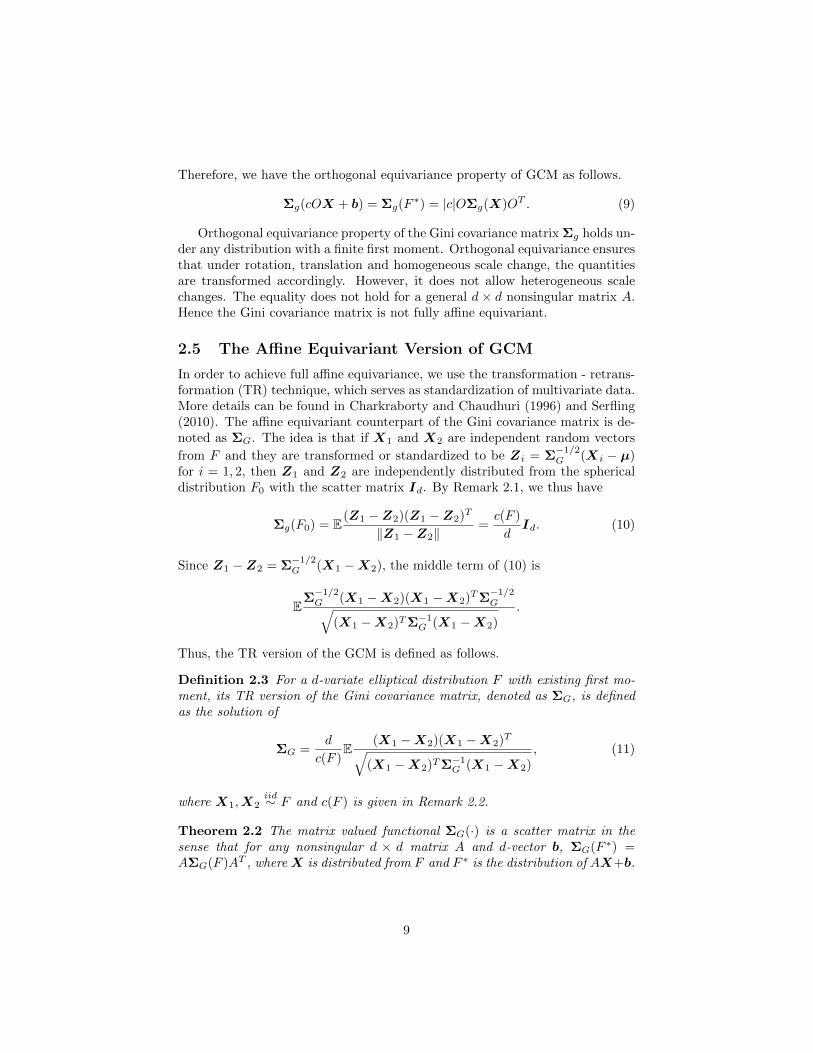
Therefore, we have the orthogonal equivariance property of GCM as follows.

Σg(cOX + b) = Σg(F∗) = |c|OΣg(X)OT . (9)

Orthogonal equivariance property of the Gini covariance matrix Σg holds un-der any distribution with a finite first moment. Orthogonal equivariance ensuresthat under rotation, translation and homogeneous scale change, the quantitiesare transformed accordingly. However, it does not allow heterogeneous scalechanges. The equality does not hold for a general d× d nonsingular matrix A.Hence the Gini covariance matrix is not fully affine equivariant.

2.5 The Affine Equivariant Version of GCM

In order to achieve full affine equivariance, we use the transformation - retrans-formation (TR) technique, which serves as standardization of multivariate data.More details can be found in Charkraborty and Chaudhuri (1996) and Serfling(2010). The affine equivariant counterpart of the Gini covariance matrix is de-noted as ΣG. The idea is that if X1 and X2 are independent random vectors

from F and they are transformed or standardized to be Zi = Σ−1/2G (Xi − µ)

for i = 1, 2, then Z1 and Z2 are independently distributed from the sphericaldistribution F0 with the scatter matrix Id. By Remark 2.1, we thus have

Σg(F0) = E(Z1 −Z2)(Z1 −Z2)T

‖Z1 −Z2‖=c(F )

dId. (10)

Since Z1 −Z2 = Σ−1/2G (X1 −X2), the middle term of (10) is

EΣ−1/2G (X1 −X2)(X1 −X2)TΣ

−1/2G√

(X1 −X2)TΣ−1G (X1 −X2)

.

Thus, the TR version of the GCM is defined as follows.

Definition 2.3 For a d-variate elliptical distribution F with existing first mo-ment, its TR version of the Gini covariance matrix, denoted as ΣG, is definedas the solution of

ΣG =d

c(F )E

(X1 −X2)(X1 −X2)T√(X1 −X2)TΣ−1

G (X1 −X2), (11)

where X1,X2iid∼ F and c(F ) is given in Remark 2.2.

Theorem 2.2 The matrix valued functional ΣG(·) is a scatter matrix in thesense that for any nonsingular d × d matrix A and d-vector b, ΣG(F ∗) =AΣG(F )AT , where X is distributed from F and F ∗ is the distribution of AX+b.

9

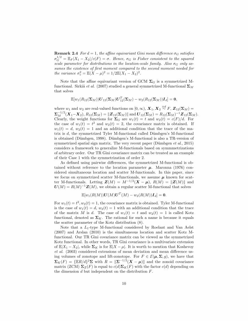
Remark 2.4 For d = 1, the affine equivariant Gini mean difference σG satisfies

σ1/2G = EF |X1 −X2|/c(F ) = σ. Hence, σG is Fisher consistent to the squared

scale parameter for distributions in the location-scale family. Also σG only as-sumes the existence of first moment compared to the second moment needed forthe variance σ2

v = E(X − µ)2 = 1/2E(X1 −X2)2.

Note that the affine equivariant version of GCM ΣG is a symmetrized M-functional. Sirkia et al. (2007) studied a general symmetrized M-functional ΣM

that solves

E[w1(R12(ΣM ))U12(ΣM )UT12(ΣM )− w2(R12(ΣM ))Id] = 0,

where w1 and w2 are real-valued functions on [0,∞), X1,X2iid∼ F , Z12(ΣM ) =

Σ−1/2M (X1−X2), R12(ΣM ) = ‖Z12(ΣM )‖ andU12(ΣM ) = R12(ΣM )−1Z12(ΣM ).

Clearly, the weight functions for ΣG are w1(t) = t and w2(t) = c(F )/d. Forthe case of w1(t) = t2 and w2(t) = 2, the covariance matrix is obtained. Ifw1(t) = d, w2(t) = 1 and an additional condition that the trace of the ma-trix is d, the symmetrized Tyler M-functional called Dumbgen’s M-functionalis obtained (Dumbgen, 1998). Dumbgen’s M-functional is also a TR-version ofsymmetrized spatial sign matrix. The very recent paper (Dumbgen et al., 2015)considers a framework to generalize M-functionals based on symmmetrizationsof arbitrary order. Our TR Gini covariance matrix can be treated as an exampleof their Case 1 with the symmetrization of order 2.

As defined using pairwise differences, the symmetrized M-functional is ob-tained without reference to the location parameter µ. Maronna (1976) con-sidered simultaneous location and scatter M-functionals. In this paper, sincewe focus on symmetrized scatter M-functionals, we assume µ known for scat-ter M-functionals. Letting Z(M) = M−1/2(X − µ), R(M) = ‖Z(M)‖ andU(M) = R(M)−1Z(M), we obtain a regular scatter M-functional that solves

E[w1(R(M))U(M)UT (M)− w2(R(M))Id] = 0.

For w1(t) = t2, w2(t) = 1, the covariance matrix is obtained. Tyler M-functionalis the case of w1(t) = d, w2(t) = 1 with an additional condition that the traceof the matrix M is d. The case of w1(t) = t and w2(t) = 1 is called Kotzfunctional, denoted as ΣK . The rational for such a name is because it equalsthe scatter parameter of the Kotz distribution (8).

Note that a L1-type M-functional considered by Roelant and Van Aelst(2007) and Arslan (2010) is the simultaneous location and scatter Kotz M-functional. Our TR Gini covariance matrix can be viewed as the symmetrizedKotz functional. In other words, TR Gini covariance is a multivariate extensionof E|X1 −X2|, while ΣK is for E|X − µ|. It is worth to mention that Koshevoyet al. (2003) considered extensions of mean deviation and mean difference us-ing volumes of zonotope and lift-zonotope. For F ∈ E(µ,Σ, g), we have that

ΣK(F ) = {ER/d}2Σ with R = ‖Σ−1/2(X − µ)‖ and the zonoid covariancematrix (ZCM) ΣZ(F ) is equal to c(d)ΣK(F ) with the factor c(d) depending onthe dimension d but independent on the distribution F .

10

Instead of taking the TR technique, Visuri et al. (2000) re-estimated eacheigenvalue of the spatial rank covariance (RCM) defined in (5) to make it affineequivariant. Yu et al. (2015) used the median of absolute deviation (MAD) toestimate scale of each univariate projected data on each of eigenvector directions.Thus the resulting RCM is affine equivariant and robust. However, it maytrade off too much efficiency for robustness. The simulation in later sectionconfirms its relatively low finite sample efficiency comparing to symmetrizedM-estimators. Also, as cautioned in Nordhausen and Tyler (2015), those robustalternatives may not have the block independence property.

2.6 Block Independence Property

One important property of symmetrized scatter functionals is the independenceproperty, or more generally, the block independence property. A scatter func-tional with the block independence property means that it is a block diagonalmatrix if the block components of the random vector are independent. Such aproperty holds naturally for the regular covariance matrix, but it may not holdfor general M-functionals and some other robust scatter functionals, as notedin Nordhausen and Tyler (2015). They proved that any symmetrized scatterfunctionals have the block independent property. In fact, such a result holdsfor any symmetrized orthogonally equivariant covariance matrix since the proofof their theorem only uses the conditions of symmetry and orthogonal equiv-ariance. As a result, our two versions of GCM have the block independenceproperty as stated in the following corollary.

Corollary 2.1 Let XT = (XT1 ,X

T2 , ...,X

Tk ) have k independent blocks with

dimensions d1, ..., dk (d1 + d2 + ... + dk = d). Then Σg(X) and ΣG(X) areblock diagonal matrices with block dimensions d1, ..., dk.

The block independence property is beneficial in many applications, for ex-ample, in independent component analysis (Oja et al., 2006), in independentsubspace analysis (Nordhausen and Oja, 2011), or in invariant coordinate selec-tion (Tyler et al., 2009).

In the next section, we study the robustness properties of the two Gini co-variance matrices along with the Kotz functional through the influence functionapproach.

3 Influence function

The influence function (IF) introduced by Hampel (1974) is a standard heuristictool for measuring the effect of infinitesimal perturbations on a functional T .For a distribution F on Rd and a covariance functional T : F 7→ T (F ) ∈ M+

withM+ being the set of d×d positive definite matrices, the IF of T at F maybe expressed as

IF(x;T, F ) = limε→0

T ((1− ε)F + εδx)− T (F )

ε, x ∈ Rd,

11

where δx denotes the point mass distribution at x. Not only is the IF a localrobustness measure of T (F ), it is also useful in deriving asymptotic efficiencyof the corresponding estimator T (Fn), where Fn is the empirical distribution.

Proposition 3.1 The influence function of the Gini covariance matrix Σg is

IF (x; Σg, F ) = 2E(X1 − x)(X1 − x)T

‖X1 − x‖− 2Σg.

Remark 3.1 For d = 1, we obtain the influence function for the Gini meandifference, that is, IF (x;σg, F ) = 2E|X1−x|−2σg, which is approximately linearfor large |x| in contrast to the quadratic form in IF (x;σ2

v , F ) = E(X1−x)2−σ2v =

(x− µ)2, the influence function of the regular variance.

The influence function of the affine equivariant GCM is more complicatedthan that of GCM. Hampel et al. (1986) showed that, for an affine equivariantscatter functional M(·), the influence function of M at a spherical distributionF0(g) in Rd is given by

IF (x;M,F0) = αM (‖x‖) xxT

‖x‖2− βM (‖x‖)Id, (12)

where αM and βM are two real valued functions depending on F0(g). Then theinfluence function of M at an elliptical distribution F (µ,Σ, g) is

IF (x;M,F ) = Σ1/2IF (Σ−1/2(x− µ);M,F0)Σ1/2.

The following corollary states the influence function of the TR version ofGCM, which is obtained as a special case of Theorem 2 in Sirkia et al. (2007)with w1(t) = t and w2(t) = c(F0)/d.

Corollary 3.1 The influence function of the affine equivariant version of theGini covariance matrix ΣG at a spherical distribution F0 is of the form (12)with

αΣG(‖x‖) =2d(d+ 2)

(d+ 1)c(F0)E[(‖X1 − ‖x‖e1‖)−

d(X1)22

‖X1 − ‖x‖e1‖

],

βΣG(‖x‖) = 4− 2d

(d+ 1)c(F0)E[(‖X1 − ‖x‖e1‖) +

(d+ 2)(X1)22

‖X1 − ‖x‖e1‖

],

where (X1)2 denotes the second coordinate of X1, e1 = (1, 0, ..., 0)T , andc(F0) = EF0

‖X1 −X2‖.

Remark 3.2 For d = 1, the influence function for σG is IF (x;σG, F0) =ασG(|x|) − βσG(|x|) = 4E|X1 − |x||/c(F0) − 4, where c(F0) = EF0 |X1 − X2|.Again, it is approximately linear in large values of |x|.

Applying the result of M-functional from Huber and Ronchetti (2009) (pp.220-222) to the Kotz functional, we have the following corollary.

12

0 2 4 6 8

05

1015

20

r

alpha

TR GiniKotzDümbgenTylerCov

0 2 4 6 8

-2-1

01

23

4

r

beta

TR GiniKotzDümbgenTylerCov

Figure 1: Functions αM (r) (left panel) and βM (r) (right panel) for covariancematrix, Tyler M functional, Dumbgen functional, Kotz functional and TR Ginicovariance matrix under the bivariate standard normal distribution.

Corollary 3.2 The influence function of Kotz functional ΣK at a sphericaldistribution F0 is of the form (12) with

αΣK (‖x‖) =d(d+ 2)

(d+ 1)c1(F0)‖x‖, βΣK (‖x‖) =

d

c1(F0)

[2− ‖x‖

d+ 1

],

where c1(F0) = EF0‖X1‖ with X1 from F0.

Remark 3.3 For a spherical distribution F0(g), c1(F0) = Er where r has thedistribution of (7).

Remark 3.4 If F0 is a spherical t distribution Td(ν) with ν > 1,

c1(F0) =ν1/2Γ[(ν − 1)/2]√

2Γ(ν/2)

√2Γ[(d+ 1)/2]

Γ(d/2).

Note that when ν → ∞, using Stirling formula Γ(ν) ≈√

2πe−ννν−1/2, we

have ν1/2Γ[(ν−1)/2]√2Γ(ν/2)

→ 1, which corresponds to the normal case in that c1(F0) =

c(F0)/√

2 as in Remark 2.3.

Remark 3.5 If F0 is the spherical Kotz distribution (8), then c1(F0) = d, themean of Gamma(d, 1).

Figure 1 displays functions αM (r) and βM (r) for covariance matrix, Tyler Mfunctional, Dumbgen functional, Kotz functional and TR Gini covariance ma-trix under the bivariate standard normal distribution. From (12), the functionα is the influence of x on an off-diagonal element of M , that is, IF (x;Mij , F0) =

13

αM (‖x‖)uiuj , where ui and uj are the ith and jth component of u = x/‖x‖.The influences of diagonal elements of M appear in both α and β functions.In other words, IF (x;Mii, F0) = αM (‖x‖)u2

i − βM (‖x‖). This means that forboundedness of the influence at off-diagonal elements, a necessary and suffi-cient condition is that the α is bounded, while for diagonal elements, one needsboundedness on both α and β. As we can see from Figure 1, the α and β func-tions of Tyler’s and Dumbgen’s M-functionals are bounded. The α function ofthe covariance matrix is quadratic in the radius r = ‖x‖, though its β functionis constant to be bounded. Both functions of the TR Gini covariance matrixare approximately linear for large r and those of the Kotz functionals are linear.This suggests that the TR Gini covariance matrix and Kotz matrix give moreprotection to moderate outliers than the covariance matrix but they are notrobust in the strict sense. The Kotz functional and its symmetrized version TRGini covariance matrix are L1 methods. They are more robust than L2 meth-ods, and also very efficient (as we will see in the next section). Such propertiesare also shared by the zonoid scatter matrix (Koshevoy et al., 2003), Oja signand rank covariance matrix (Ollila et al., 2003; Ollila et al., 2004). They allhave influence functions linear or approximately linear in r.

Note that the influence function of the affine equivariant version of spatialrank covariance matrix (MRCM) considered by Visuri et al. (2000) can notbe written as the form of (12) because of the construction way of MRCM withnonlinear transformations. See Yu et al. (2015) for more details.

4 Estimation

4.1 Sample Gini Covariance Matrix

Suppose that X = {X1, ...,Xn} is a random sample from a continuous distribu-tion F in Rd and its empirical distribution is Fn. Then the sample counterpartof the Gini covariance matrix is obtained by replacing F with the empiricaldistribution Fn in (4). That is,

Σg = Σg(Fn) =2

n

n∑i=1

Xir(Xi)T =

(n

2

)−1∑i<j

(Xi −Xj)(Xi −Xj)T

‖Xi −Xj‖. (13)

Clearly, the sample Gini covariance matrix Σg(Fn) is a matrix-valued U -statisticUn to estimate Σg(F ) with the kernel h(x1,x2) = (x1−x2)(x1−x2)T /‖x1−x2‖.A straightforward generalization of univariate results on non-degenerated U -statistics given in Serfling (1980) establishes

√n-consistency of Σg(Fn). This

means that for F having a finite second moment,

√n(Σg −Σg) =

√n(Un −Σg) =

√n

[1

n

n∑i=1

IF (Xi; Σg, F )

]+Rn, (14)

where the remainder term satisfies Rnp→ 0. We have the following proposition.

14

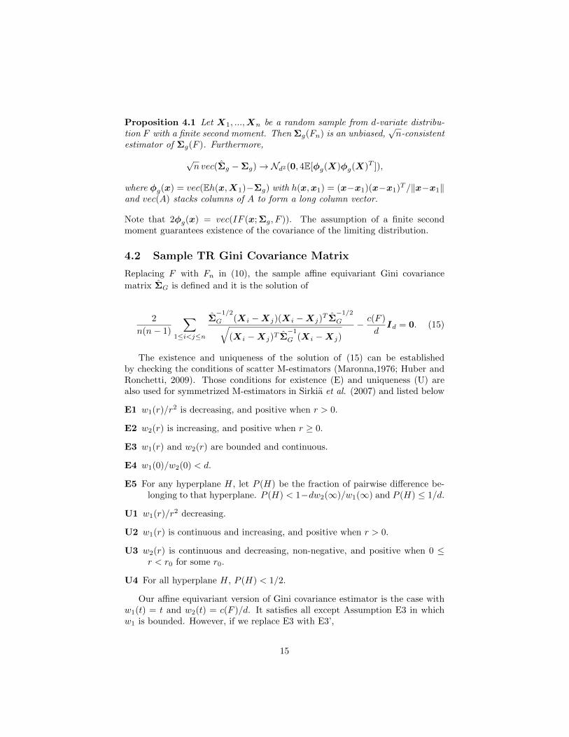
Proposition 4.1 Let X1, ...,Xn be a random sample from d-variate distribu-tion F with a finite second moment. Then Σg(Fn) is an unbiased,

√n-consistent

estimator of Σg(F ). Furthermore,

√n vec(Σg −Σg)→ Nd2(0, 4E[φg(X)φg(X)T ]),

where φg(x) = vec(Eh(x,X1)−Σg) with h(x,x1) = (x−x1)(x−x1)T /‖x−x1‖and vec(A) stacks columns of A to form a long column vector.

Note that 2φg(x) = vec(IF (x; Σg, F )). The assumption of a finite secondmoment guarantees existence of the covariance of the limiting distribution.

4.2 Sample TR Gini Covariance Matrix

Replacing F with Fn in (10), the sample affine equivariant Gini covariance

matrix ΣG is defined and it is the solution of

2

n(n− 1)

∑1≤i<j≤n

Σ−1/2

G (Xi −Xj)(Xi −Xj)T Σ−1/2

G√(Xi −Xj)T Σ

−1

G (Xi −Xj)

− c(F )

dId = 0. (15)

The existence and uniqueness of the solution of (15) can be establishedby checking the conditions of scatter M-estimators (Maronna,1976; Huber andRonchetti, 2009). Those conditions for existence (E) and uniqueness (U) arealso used for symmetrized M-estimators in Sirkia et al. (2007) and listed below

E1 w1(r)/r2 is decreasing, and positive when r > 0.

E2 w2(r) is increasing, and positive when r ≥ 0.

E3 w1(r) and w2(r) are bounded and continuous.

E4 w1(0)/w2(0) < d.

E5 For any hyperplane H, let P (H) be the fraction of pairwise difference be-longing to that hyperplane. P (H) < 1−dw2(∞)/w1(∞) and P (H) ≤ 1/d.

U1 w1(r)/r2 decreasing.

U2 w1(r) is continuous and increasing, and positive when r > 0.

U3 w2(r) is continuous and decreasing, non-negative, and positive when 0 ≤r < r0 for some r0.

U4 For all hyperplane H, P (H) < 1/2.

Our affine equivariant version of Gini covariance estimator is the case withw1(t) = t and w2(t) = c(F )/d. It satisfies all except Assumption E3 in whichw1 is bounded. However, if we replace E3 with E3’,

15

E3’ The distribution of F has a finite first moment,

then Lemma 8.3 in Huber and Ronchetti (2009) is still satisfied, hence ourestimator does exist and exists uniquely. The assumption E3’ is in agreementwith the condition of Dumbgen et al. (2015) for the Case 1 in which ψ(t) =

√t.

Intuitively, we can find the solution of the equation of (15) by a commoniterative algorithm:

Σ(t+1)

G ←− 2

n(n− 1)

d

c(F )

∑1≤i<j≤n

(xi − xj)(xi − xj)T√(xi − xj)T (Σ

(t)

G )−1(xi − xj). (16)

The initial value can take Σ(0)

G = Id. The iteration stops when ‖Σ(t+1)

G −Σ

(t)

G ‖ < ε for a pre-specified number ε > 0, where ‖ · ‖ can take any matrixnorm. Note that we need to know the distribution F since c(F ) is includedin (16). In this case the estimator is Fisher consistent to Σ. Usually onemakes the estimator Fisher consistent at the normal model. That is, one takesc(F ) = 2Γ[(d + 1)/2]/Γ(d/2) as stated in Remark 2.3. If one is interested inestimation of correlation matrix or shape matrix (shape matrix is defined laterat Section 4.3), there is no need to specify the distribution. One can delete thefactor d/c(F ) in the equation of (15) and obtain its solution for estimation ofscatter matrix up to a factor.

The above algorithm is called the fixed-point algorithm and its convergencefrom any start points has been rigorously proved (Tyler, 1987). However, itcan be rather slow for high dimensions and large sample sizes. The very recentpaper by Dumbgen, Nordhausen and Schuhmacher (2016) provide much fasternew algorithms by utilizing a Taylor expansion of second order of the targetfunctional. For large n, they approximate symmetrized estimators by consid-ering the surrogate ones rather than all pairwise differences. Based on theiridea, an algorithm for our Gini estimator can be developed and added to theirR package “fastM” (Dumbgen et al., 2014).

If we assume that the location parameter µ is known, then the MLE of Σin the Kotz distribution (8) is found to be a scatter M-estimator, which is the

solution of Σ in the equation below:

1

n

n∑i=1

(Xi − µ)(Xi − µ)T√(Xi − µ)T Σ

−1(Xi − µ)

= Σ. (17)

The solution of Σ in (17) is denoted as ΣK , which is ΣK(Fn). Assuming aknown location parameter is for avoiding some restrictive regularity conditionsfor the simultaneous M-estimators. The simultaneous one is treated in Roelantand Van Aelst (2007) and Arslan (2010). Our TR version GCM estimator is thesymmetrized scatter MLE of the Kotz distribution without the need of referenceto the location parameter, and hence avoids the above situation.

Dumbgen et al. (2015) provided a general treatment and asymptotics forM-estimation of multivariate scatter. The Kotz and TR Gini estimators are

16

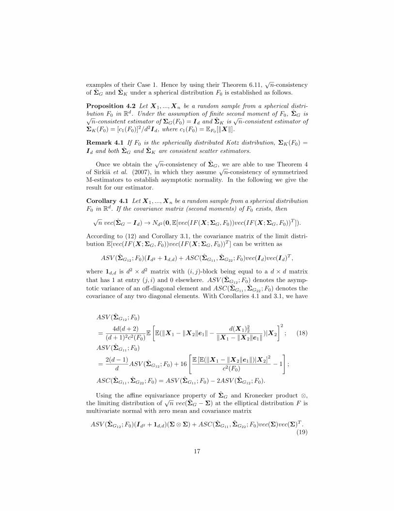
examples of their Case 1. Hence by using their Theorem 6.11,√n-consistency

of ΣG and ΣK under a spherical distribution F0 is established as follows.

Proposition 4.2 Let X1, ...,Xn be a random sample from a spherical distri-bution F0 in Rd. Under the assumption of finite second moment of F0, ΣG is√n-consistent estimator of ΣG(F0) = Id and ΣK is

√n-consistent estimator of

ΣK(F0) = [c1(F0)]2/d2Id, where c1(F0) = EF0 [‖X‖].

Remark 4.1 If F0 is the spherically distributed Kotz distribution, ΣK(F0) =

Id and both ΣG and ΣK are consistent scatter estimators.

Once we obtain the√n-consistency of ΣG, we are able to use Theorem 4

of Sirkia et al. (2007), in which they assume√n-consistency of symmetrized

M-estimators to establish asymptotic normality. In the following we give theresult for our estimator.

Corollary 4.1 Let X1, ...,Xn be a random sample from a spherical distributionF0 in Rd. If the covariance matrix (second moments) of F0 exists, then

√n vec(ΣG − Id)→ Nd2(0,E[vec(IF (X; ΣG, F0))vec(IF (X; ΣG, F0))T ]).

According to (12) and Corollary 3.1, the covariance matrix of the limit distri-bution E[vec(IF (X; ΣG, F0))vec(IF (X; ΣG, F0))T ] can be written as

ASV (ΣG12;F0)(Id2 + 1d,d) +ASC(ΣG11

, ΣG22;F0)vec(Id)vec(Id)

T ,

where 1d,d is d2 × d2 matrix with (i, j)-block being equal to a d × d matrix

that has 1 at entry (j, i) and 0 elsewhere. ASV (ΣG12 ;F0) denotes the asymp-

totic variance of an off-diagonal element and ASC(ΣG11, ΣG22

;F0) denotes thecovariance of any two diagonal elements. With Corollaries 4.1 and 3.1, we have

ASV (ΣG12 ;F0)

=4d(d+ 2)

(d+ 1)2c2(F0)E[E(‖X1 − ‖X2‖e1‖ −

d(X1)22

‖X1 − ‖X2‖e1‖)|X2

]2

; (18)

ASV (ΣG11;F0)

=2(d− 1)

dASV (ΣG12 ;F0) + 16

[E [E(‖X1 − ‖X2‖e1‖)|X2]

2

c2(F0)− 1

];

ASC(ΣG11 , ΣG22 ;F0) = ASV (ΣG11 ;F0)− 2ASV (ΣG12 ;F0).

Using the affine equivariance property of ΣG and Kronecker product ⊗,the limiting distribution of

√n vec(ΣG −Σ) at the elliptical distribution F is

multivariate normal with zero mean and covariance matrix

ASV (ΣG12;F0)(Id2 + 1d,d)(Σ⊗Σ) +ASC(ΣG11

, ΣG22;F0)vec(Σ)vec(Σ)T .

(19)

17

Checking the conditions (N1-N4) of MLE proposed by Huber (1967), we are

able to establish the normality of Kotz estimator ΣK assuming a known locationparameter.

Proposition 4.3 Let X1, ...,Xn be a random sample from spherical distribu-tion F0(g) in Rd. If the second moment of F0(g) exists and the first moment isknown, then

√n vec(ΣK −ΣK)→ Nd2(0,E[vec(IF (X; ΣK , F0))vec(IF (X; ΣK , F0))T ]).

With the results of Corollary 3.2 and Proposition 4.3, we have

ASV (ΣK12;F0) =

d(d+ 2)EF0 [‖X‖2]

(d+ 1)2[c1(F0)]2, (20)

in which EF0 [‖X‖2] = ER2 with R having the distribution of (7).

4.3 Asymptotic Efficiency

Although our TR Gini covariance estimator is Fisher consistent to the scat-ter matrix since it is corrected by c(F0)/d, we consider its shape estimator inorder to compare its limiting efficiency with that of the Tyler and DumbgenM-estimators. The shape matrix associated with the scatter functional Σ is

W (F ) =d

Tr(Σ(F ))Σ(F ).

Note that there are also other definitions for a shape matrix. For example,Paindaveine (2008) uses the determinant. Here we use the shape matrix basedon the matrix trace because it allows us to compare asymptotic efficiency moreeasily. Tyler and Dumbgen estimators estimate the shape matrix. At ellipticaldistributions, all shape estimators estimate the same population quantity andhence are comparable without any correction factors. Theorem 5 of Sirkia etal. (2007) states that a single number characterizes the limiting distributionof the shape estimators at F0 and that number is the variance of off-diagonalelements of Σ or W , τ . In general, the asymptotic relative efficiency (ARE)of an estimator T1 with respect to another estimator T2 is defined as the ratioof ASV (T2) and ASV (T1). Hence for shape estimators, the ARE of W1 withrespect to W2 is τ(W2)/τ(W1).

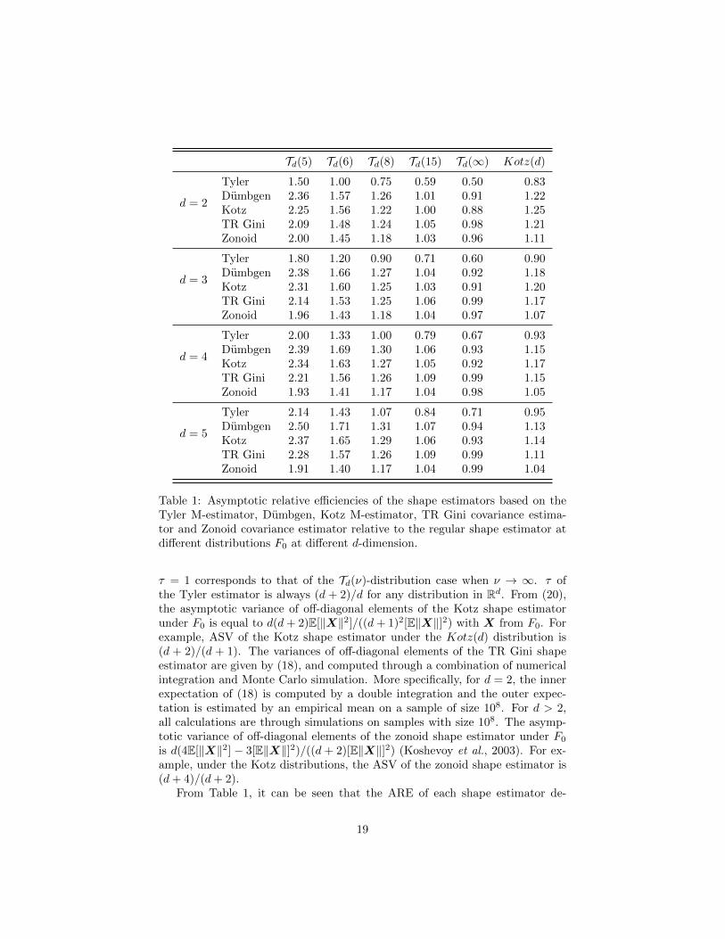
Listed in Table 1 are the limiting efficiencies of shape estimators with re-spect to the shape estimator based on the regular sample covariance matrix(i.e. the regular shape estimator). The efficiencies are considered under spheri-cal Kotz(d) distribution and Td(ν) distributions at different dimensions d withdifferent degrees of freedom ν, with ν = ∞ referring to the normal case. Thevariance of the off-diagonal element of the regular shape estimator at F0 equalto 1 + κ(F0), where κ(F0) is the kurtosis of F0. That is, τ of the regular shapeestimator is (ν−2)/(ν−4) in the Td(ν)-distributions for ν > 4 and (d+3)/(d+1)in the Kotz(d) distribution (Wang, 2009; Zografos, 2008). In the normal case,

18

Td(5) Td(6) Td(8) Td(15) Td(∞) Kotz(d)

d = 2

Tyler 1.50 1.00 0.75 0.59 0.50 0.83Dumbgen 2.36 1.57 1.26 1.01 0.91 1.22Kotz 2.25 1.56 1.22 1.00 0.88 1.25TR Gini 2.09 1.48 1.24 1.05 0.98 1.21Zonoid 2.00 1.45 1.18 1.03 0.96 1.11

d = 3


d = 4


d = 5


Table 1: Asymptotic relative efficiencies of the shape estimators based on theTyler M-estimator, Dumbgen, Kotz M-estimator, TR Gini covariance estima-tor and Zonoid covariance estimator relative to the regular shape estimator atdifferent distributions F0 at different d-dimension.

τ = 1 corresponds to that of the Td(ν)-distribution case when ν → ∞. τ ofthe Tyler estimator is always (d + 2)/d for any distribution in Rd. From (20),the asymptotic variance of off-diagonal elements of the Kotz shape estimatorunder F0 is equal to d(d+ 2)E[‖X‖2]/((d+ 1)2[E‖X‖]2) with X from F0. Forexample, ASV of the Kotz shape estimator under the Kotz(d) distribution is(d + 2)/(d + 1). The variances of off-diagonal elements of the TR Gini shapeestimator are given by (18), and computed through a combination of numericalintegration and Monte Carlo simulation. More specifically, for d = 2, the innerexpectation of (18) is computed by a double integration and the outer expec-tation is estimated by an empirical mean on a sample of size 108. For d > 2,all calculations are through simulations on samples with size 108. The asymp-totic variance of off-diagonal elements of the zonoid shape estimator under F0

is d(4E[‖X‖2] − 3[E‖X‖]2)/((d + 2)[E‖X‖]2) (Koshevoy et al., 2003). For ex-ample, under the Kotz distributions, the ASV of the zonoid shape estimator is(d+ 4)/(d+ 2).

From Table 1, it can be seen that the ARE of each shape estimator de-

19

creases as ν increases in Td(ν) distributions, and the ARE of Tyler, Dumbgen,Kotz and TR Gini shape estimators increases as dimension d increases. In thenormal cases, TR Gini estimator has a 98% ARE for d = 2 and 99% for d ≥ 3.With very little loss in efficiency in the normal case, the TR Gini estimator gainsefficiency in the heavy tailed distributions. For example, its ARE is greater than2 relative to the regular shape estimator in the Td(5) distribution. The Tylerestimator has the lowest ARE among all estimators except the Zonoid estima-tor for all distributions considered. In particular, the symmetrized Dumbgenestimator is more efficient than its counterpart, the Tyler estimator, in all dis-tributions. However, such a result does not hold for all symmetrized estimators.TR Gini shape estimator is more efficient than Kotz estimator in Td(15) andTd(∞), but less efficient in the Kotz and Td(ν) distributions with ν = 5, 6. Itis worthwhile to point out that Gerstenberger and Vogel (2015) studied effi-ciency of Gini mean difference. Their results complement ours for Kotz and TRGini estimator when d = 1. The ARE’s of the zonoid shape estimator underTd(∞) are 0.96, 0.97, 0.98 and 0.99, respectively for d = 2, 3, 4, 5. Under T2(ν),their ARE’s are 2.00, 1.45, 1.18 and 1.03, respectively for ν = 5, 6, 8, 15. Thosenumbers are similar to (slightly smaller than) the ARE’s of our TR Gini shapeestimator, which is not surprising since both are multivariate extensions of themean deviation or mean difference and both have linear or approximately linearinfluence functions. They are highly efficient at the normal and fairly robustat the heavy-tailed cases. For Td(5), Td(6), Td(8) and Kotz distributions, theefficiency of the Zonoid shape estimator decreases with d, which is different fromother estimators. At T5(5), the Zonoid shape estimator is least efficient amongM-estimators and symmetrized M-estimators, but it is much efficient than theregular shape estimator.

4.4 Finite Sample Efficiency

We conduct a small simulation to study finite sample efficiencies of the shapeestimators with respect to the regular shape estimator. M = 10000 samples oftwo different sample sizes (n = 50, 200) at two different dimensions (d = 2, 5) aredrawn from spherical T -distributions with 5, 8 and ∞ degrees of freedoms andfrom spherical Kotz distribution. We use R Package “mnormt” (Azzalini andGenz, 2016) to generate samples from multivariate T -distributions and normaldistribution. We generate a random vector X from spherical Kotz distributionby X = RU , in which R is distributed from the Gamma distribution with theshape parameter being d and the scale parameter being 1 and U = Z/‖Z‖ withZ being a vector formed by d iid standard normal variables. If a random samplefrom Kotz(µ,Σ) is required, then by taking Σ’s Cholesky decomposition L, wehave Y = LX + µ from Kotz(µ,Σ).

In the simulation, all M-estimators and symmetrized M-estimators are cal-culated by the fixed-point algorithm. Tyler and Kotz shape estimators use thetrue location values in the computation. tyler.shape and duembgen.shape func-tions in R package “ICSNP” (Nordhausenet al., 2015) are used for computingTyler and Dumbgen estimators. Also spatial.rank function of “ICSNP” is used

20

Td(5) Td(8) Td(∞) Kotz(d)

n\d 2 5 2 5 2 5 2 5

Tyler 50 0.81 1.12 0.61 0.71 0.45 0.49 0.71 0.75200 1.14 1.60 0.82 1.01 0.59 0.69 0.79 0.90∞ 1.50 2.14 0.75 1.07 0.50 0.71 0.83 0.95

Dumbgen 50 1.27 1.73 1.02 1.15 0.83 0.89 1.04 0.94200 1.35 1.88 1.03 1.23 0.81 0.91 1.17 1.09∞ 2.36 2.50 1.26 1.31 0.91 0.89 1.22 1.13

Kotz 50 1.41 1.72 1.15 1.19 0.91 0.96 1.23 1.13200 1.54 1.87 1.22 1.27 0.95 0.94 1.24 1.14∞ 2.25 2.37 1.22 1.29 0.88 0.93 1.25 1.14

TR Gini 50 1.31 1.60 1.14 1.18 0.98 0.99 1.15 1.09200 1.36 1.67 1.16 1.21 0.99 0.99 1.18 1.10∞ 2.09 2.28 1.24 1.26 0.98 0.99 1.21 1.11

MRCM 50 0.95 1.17 0.72 0.71 0.52 0.49 0.78 0.75200 1.29 1.50 0.92 0.92 0.63 0.60 0.84 0.81

(Qn) 200 1.65 1.83 1.11 1.19 0.83 0.87 1.07 1.04

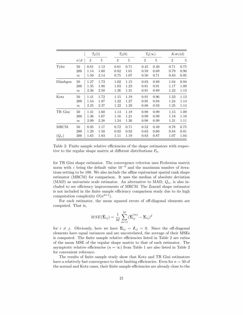
Table 2: Finite sample relative efficiencies of the shape estimators with respec-tive to the regular shape matrix at different distributions F0.

for TR Gini shape estimator. The convergence criterion uses Frobenius matrixnorm with ε being the default value 10−6 and the maximum number of itera-tions setting to be 100. We also include the affine equivariant spatial rank shapeestimator (MRCM) for comparison. It uses the median of absolute deviation(MAD) as univariate scale estimator. An alternative to MAD, Qn, is also in-cluded to see efficiency improvements of MRCM. The Zonoid shape estimatoris not included in the finite sample efficiency comparison study due to its highcomputation complexity O(nd+1).

For each estimator, the mean squared errors of off-diagonal elements arecomputed. That is,

MSE(Σij) =1

M

M∑m=1

(Σ(m)

ij −Σij)2

for i 6= j. Obviously, here we have Σij = Iij = 0. Since the off-diagonalelements have equal variances and are uncorrelated, the average of their MSEsis computed. The finite sample relative efficiencies listed in Table 2 are ratiosof the mean MSE of the regular shape matrix to that of each estimator. Theasymptotic relative efficiencies (n =∞) from Table 1 are also listed in Table 2for convenient reference.

The results of finite sample study show that Kotz and TR Gini estimatorshave a relatively fast convergence to their limiting efficiencies. Even for n = 50 ofthe normal and Kotz cases, their finite sample efficiencies are already close to the

21

asymptotic ones. For the Tyler estimator, the convergence is slower, and the lossin efficiency is larger for finite sample sizes comparing to that of others. In thecase of the T (5) distribution, the convergence to the limiting efficiency is muchslower than that of the other cases. Low efficiency of MRCM can be explainedby low efficiency of the univariate scale estimator MAD. Improvement can bedone by using other robust alternatives which are more efficient, as suggestedby Rousseeuw and Croux (1993). They recommended Qn which is given bythe 0.25 quantile of the pairwise distances multiplying some correction factor.For the normal distribution under the size n = 200, if Qn is used, the RE ofMRCM increases to 0.83 for d = 2 and 0.87 for d = 5. Similar improvementsare observed for other distributions also.

5 Conclusion

We have extended the univariate Gini mean difference to the multivariate caseand proposed two versions of Gini covariance matrix (GCM). New covariancematrices are based on pairwise differences. Thus the location center needs notbe estimated nor known. Their properties have been explored. They possess theblock independence property, which allow them beneficial in many applications.Their influence functions have been derived. It was found that the influencefunctions of GCM are approximately linear, which is unbounded. In a strictsense, they are not highly robust. However, they are highly efficient undernormal distributions. They have greater than 98% asymptotic relative efficiencywith respect to sample covariance matrix. On the other hand, they are morerobust than the covariance matrix which has influence function of a quadraticform. GCM will give more protection to moderate outliers than the covariancematrix. Similar properties are also shared by the Oja sign or rank covariancematrix and the zoniod or lift-zoniod covariance matrix, but our proposed onesenjoy computational ease. Hence the proposed affine equivariant GCM providesus an option for estimating scatter matrix with a consideration to balance wellamong efficiency, robustness and computation.

6 Appendix

Proof of Theorem 2.1. We first show that X1−X2 is elliptically distributedwith center 0 and scatter parameter 2Σ by its characteristic function as follows.

EeitT

(X1−X2) = EeitTX1Ee−it

TX2 = eitTµe−it

Tµψ2(tTΣt) := ψ∗(2tTΣt),

where ψ∗(s) = ψ2(s/2). Note that except for normal distributions, X1 −X2

has a different generating function g∗ from g, the one for X.Let Zi = V T (Xi − µ) for i = 1, 2, then Z1 − Z2 = V T (X1 − X2) fol-

lows a centered elliptical distribution with diagonal scatter matrix 2Λ. Wecan write (2Λ)−1/2(Z1 − Z2) = RU with R = ‖(2Λ)−1/2(Z1 − Z2)‖ and

22

U = (2Λ)−1/2(Z1 − Z2)/R being independent with R and uniformly distri-bution on the unit sphere. Then

Σg = E[

(X1 −X2)(X1 −X2)T

‖X1 −X2‖

]= V E

[(Z1 −Z2)(Z1 −Z2)T

‖Z1 −Z2‖

]V T

= V E

[2R2Λ1/2UUTΛ1/2√2R2UTΛ1/2Λ1/2U

]V T =

√2ERV E

[Λ1/2UUTΛ1/2√

UTΛU

]V T .

Denote√

2ER as c(F ), the proof is complete. �

Proof of Theorem 2.2. Multiplying A on the left and AT on the right toboth sides of Equation (11), we have

AΣGAT =

d

c(F )EA(X1 −X2)(X1 −X2)TAT√

(X1 −X2)TΣ−1G (X1 −X2)

.

Since A is nonsingular, A−1 and (AT )−1 exist. Hence

AΣGAT =

d

c(F )E

A(X1 −X2)(X1 −X2)TAT√(X1 −X2)TAT (AΣGAT )−1A(X1 −X2)

.

It means that AΣGAT is the TR version of Gini covariance matrix for AX + b,

where X is random vector from distribution F . �

Proof of Proposition 3.1. The proof is straightforward. Let Y 1 and Y 2 beindependently distributed from Fε = (1− ε)F + εδx and X1 and X2 indepen-dently distributed from F , then we have

Σg(Fε) = EFε(Y 1 − Y 2)s(Y 1 − Y 2)T

= (1− ε)2EF(X1 −X2)(X1 −X2)T

‖X1 −X2‖+ 2ε(1− ε)EF

(X1 − x)(X1 − x)T

‖X1 − x‖.

Then the result for IF (x; Σg, F ) follows. �

Proof of Corollary 3.1. The affine equivariant version of Gini covariancematrix ΣG is a symmetrized M-functional with w1(t) = t and w2(t) = c(F )/d =c(F0)/d. From Theorem 2 of Sirkia et al. (2007), we get

η1 =(d+ 1)E[‖X1 −X2‖]

2d(d+ 2)=

(d+ 1)c(F0)

2d(d+ 2),

η2 =E‖X1 −X2‖

4d=c(F0)

4d.

Thus, the result is obtained. �

23

Proof of Corollary 3.2. We have the influence function of M-functional Min the form IF (x;M,F0) = −2W where W = M−1/2, W = IF (x;W,F0), and

1

dtr(W ) = −

1dw1(‖x‖)− w2(‖x‖)

E[( 1dw

′1(‖Y ‖)− w′

2(‖Y ‖))‖Y ‖],

W − 1

dtr(W )Id = −d+ 2

2

w1(‖x‖)(xxT

‖x‖2 −1dId)

Ey[w1(‖Y ‖) + 1dw

′1(‖Y ‖)‖Y ‖]

,

where Y is a random vector from the distribution F0 (see pages 220-222 ofHuber and Ronchetti (2009)).

With w1(t) = t and w2(t) = 1 along with w′

1(t) = 1 and w′

2(t) = 0 for ΣK ,solving for W in the above equations we get

W =−d(d+ 2)

2(d+ 1)E‖Y ‖‖x‖ xx

T

‖x‖2+

d+ 2

2(d+ 1)E‖Y ‖‖x‖Id −

‖x‖ − dE‖Y ‖

Id.

Let c1(F0) = E‖Y ‖. Therefore, we obtain

IF (x; ΣK , F0) = −2W

=d(d+ 2)

(d+ 1)c1(F0)‖x‖ xx

T

‖x‖2+

d

(d+ 1)c1(F0)‖x‖Id −

2d

c1(F0)Id.

Hence the result follows. �

Proof of Proposition 4.1. We only prove the asymptotic normality result.The normality of an U-statistic follows from the central limit theorem on

its first order Hoeffding decomposition provided that the U-statistic is non-degenerated. Here we need to show that E[φg(X)φg(X)T ] > 0 and exists. Theexistence is guaranteed by the assumption of finite second moment. Hence it issufficient to prove that φg(X) is of full rank almost everywhere. This is true ifP (X ∈ V ) = 0 for any proper linear subspace V (dim(V ) < d). Particularly,this is true for continuous distribution F . �

Proof of Proposition 4.2. Kotz and TR Gini estimators are examples ofthe Case 1 considered in Dumbgen et al. (2015) with the symmetrization order1 and 2, respectively. Using the same notations of Dumbgen et al. (2015),Kotz and TR Gini estimators are the cases with ρ(s) =

√s, ψ(s) = 1

2

√s and

ψ2(s) = 14

√s, which satisfy all conditions on ρ, ψ and ψ2. Under continuous

distribution F0 with finite second moments, Theorem 6.11 holds for Kotz and TRGini estimators, and hence they are

√n consistent to ΣK and ΣG, respectively.

�

Proof of Proposition 4.3. Proposition 4.3 follows if the conditions (N1-N4)by Huber (1967) are fulfilled. The notation of this proof will be chose to matchHuber’s paper. Let M+ denote the set of symmetric positive definite d × d

24

matrices. For A ∈M+, we define its norm ‖A‖ as the spectral norm of A, thatis λ1, where λ1 ≥ λ2 ≥ ... ≥ λd are eigenvalues of A. Without loss of generality,assume µ = 0. It is clear that the Kotz estimator ψ(x,M) in Huber’s papertakes the form of

ψ(x,M) = (xTM−1x)−1/2xxT −M.

Let λ(M) = Eψ(X,M) so that the true parameter Id is defined as λ(Id) = 0.Define

U(x,M, δ) = sup‖M1−M‖<δ

‖ψ(x,M1)− ψ(x,M)‖.

According to Huber’s Theorem 3 and its corollary, if there exist positive numberb, c and δ0 such that EU(X,M, δ) < bδ and EU2(X,M, δ) < cδ for ‖M −Id‖ + δ < δ0 and if E(‖ψ(X, Id)‖2) is nonzero and finite, then the asymptoticnormality of ΣK follows.

Note that U(x,M, δ) is less than

δ +‖xxT ‖‖x‖

sup‖M1−M‖<δ

|(xTM−1

1 x

xTx)−1/2 − (

xTM−1x

xTx)−1/2|.

Hence, for sufficient small δ, EU(X,M, δ) < δ+E‖X‖/dmax(√λ1 + δ−

√λd,√λ1−√

λd − δ), where λ1 and λd are the largest and smallest eigenvalues of M , respec-tively. Since ‖M−Id‖ ≤ δ0−δ, we have λ1 < 1+δ0−δ and λd > 1−δ0+δ. Thus,EU(X,M, δ) < δ+E‖X‖/dmax(

√1 + δ0−

√1− δ0 + δ,

√1 + δ0 − δ−

√1− δ0),

and it exists a b > 0 such that EU(X,M, δ) < bδ. Similarly, the existence of ccan be proved under the assumption of finite second moment, that E‖X‖2 <∞.Also the result that E(‖ψ(X, Id)‖2) is nonzero and finite follows for continuousF0 with a finite second moment.

References

[1] Arslan, O. (2010). An alternative multivariate skew Laplace distribution:properties and estimation. Statistical Papers, 51, 865-887.

[2] Azzalini, A. and Genz, A. (2016). The R package ‘mnormt’:The multivariate normal and ‘t’ distributions (version 1.5-4). URLhttp://azzalini.stat.unipd.it/SW/Pkg-mnormt

[3] Carcea, M. and Serfling, R. (2015). A Gini autocovariance function for timeseries modeling. Journal of Time Series Analysis, 36, 817-838.

[4] Chakraborty, B. and Chaudhuri, P. (1996). On a transformation and re-transformation technique for constructing an affine equivariant multivariatemedian. Proceedings of the American Mathematical Society, 124(8), 2539-2547.

25

[5] Croux, C., Ollila, E., and Oja, H. (2002). Sign and rank covariance matrices:statistical properties and application to principal components analysis, InStatistical Data Analysis Based on the L1-Norm and Related Methods, Y.Dodge (Eds.), Birkhauser, Basel, 257-271.

[6] Dumbgen, L. (1998). On Tyler’s M-functional of scatter in high dimension.Annals of Institute of Statistical Mathematics, 50, 471-491.

[7] Dumbgen, L., Nordhausen, K. and Schuhmacher, H. (2014). fastM:Fast Computation of Multivariate M-estimators. R package version 0.0-2.https://CRAN.R-project.org/package=fastM

[8] Dumbgen, L., Nordhausen, K. and Schuhmacher, H. (2016). New algo-rithms for M-estimation of multivariate scatter and location. Journal ofMultivariate Analysis, 144, 200-217.

[9] Dumbgen, L., Pauly, M. and Schweizer, T. (2015). M-functionals of multi-variate scatter. Statistics Surveys, 9, 32-105.

[10] Fang, K.T., and Anderson, T. W. (1990). Statistical Inference in EllipticallyContoured and Related Distributions, Allerton Press, New York.

[11] Gerstenberger, C. and Vogel, D. (2015). On the efficiency of Gini’s meandifference. Statistical Methods and Applications, 24(4), 569-596.

[12] Gini, C. (1914). Reprinted: On the measurement of concentration andvariability of characters (2005), Metron, LXIII(1), 3-38.

[13] Hampel, F.R. (1974). The influence curve and its role in robust estimation.Journal of American Statistics Association, 69, 383-393.

[14] Hampel, F.R., Ronchetti, E.M., Rousseeuw, P.J. and Stahel, W.J. (1986).Robust Statistics: The Approach Based on Influence Functions. Wiley, NewYork.

[15] Huber, P.J. (1967). The behavior of maximum likelihood estimates un-der nonstandard conditions, Proceedings of Fifth Berkeley Symposium onMathematical Statistics and Probability, 1, 221-233.

[16] Huber, P.J. and Ronchetti, E.M. (2009). Robust Statistics, 2nd edition.Wiley, New York.

[17] Hyvarinen, A., Karhunen, J. and Oja, E. (2001). Independent ComponentAnalysis. Wiley, New York.

[18] Koltchinskii, V.I. (1997). M-estimation, convexity and quantiles. Annals ofStatistics, 25, 435-477.

[19] Koshevoy, G. and Mosler, K. (1997). Multivariate Gini indices. Journal ofMultivariate Analysis, 60, 252-276.

26

[20] Koshevoy, G., Mottonen, J. and Oja, H. (2003). Scatter matrix estimatebased on the zonotope. Annals of Statistics, 31, 1439-1459.

[21] Kotz, S. (1975). Multivariate distributions at a cross-road. In StatisticalDistributions in Scientific Work, 1 (eds Patil, Kotz and Ord), Reidel Pub-lication Company.

[22] Maronna, R.A. (1976). Robust M-estimators of multivariate location andscatter. Annals of Statistics, 4, 51–67.

[23] Mottonen J., Oja, H. and Tienari J. (1997). On the efficiency of multivariatespatial sign and rank tests. Annals of Statistics, 25, 542-552.

[24] Nadarajah, S. (2003). The Kotz-type distribution with applications. Statis-tics, 37, 341-358.

[25] Nair, U. (1936). The standard error of Gini’s mean difference. Biometrika,28, 428-436.

[26] Nordhausen, K. and Oja, H. (2011). Scatter matrices with independentblock property and ISA. In Proceedings of the 19th European Signal Pro-cessing Conference (EUSIPCO 2011).

[27] Nordhausen, K., Sirkia, S., Oja, H. and Tyler, D.E. (2015). IC-SNP: Tools for Multivariate Nonparametrics. R package version 1.1-0.https://CRAN.R-project.org/package=ICSNP

[28] Nordhausen, K. and Tyler, D.E. (2015). A cautionary note on robust co-variance plug-in methods. Biometrika, 102, 573-588.

[29] Oja, H. (1983). Descriptive statistics for multivariate distributions. Statis-tics & Probability Letters, 1, 327-332.

[30] Oja, H. (2010). Multivariate Nonparametric Methods with R: An ApproachBased on Spatial Signs and Ranks. Springer, New York.

[31] Oja, H., Sirkia, S. and Eriksson, J. (2006). Scatter matrices and indepen-dent component analysis. Austrian Journal of Statistics, 35, 175-189.

[32] Ollila, E., Croux, C. and Oja, H. (2004). Influence function and asymptoticefficiency of the affine equivariant rank covariance matrix. Statistica Sinica,14, 297-316.

[33] Ollila, E., Oja, H. and Croux, C. (2003). The affine equivariant sign covari-ance matrix: Asymptotic behavior and efficiencies. Journal of MultivariateAnalysis, 87, 328-355.

[34] Paindaveine, D. (2008). A canonical definition of shape. Statistics and Prob-ability Letters, 78, 2240-2247.

27

[35] Roelant, E. and Van Aelst, S. (2007). An L1-type estimator of multivariatelocation and shape. Statistical Methods and Applications, 15, 381-393.

[36] Rousseeuw, P.J. and Croux, C. (1993). Alternatives to the median absolutedeviation. Journal of the American Statistical Association, 88, 1273-1283.

[37] Serfling, R. (1980). Approximation Theorems of Mathematical Statistics.Wiley.

[38] Serfling, R. (2010). Equivariance and invariance properties of multivariatequantile and related functions, and the role of standardization. Journal ofNonparametric Statistics, 22, 915-936.

[39] Serfling, R. and Xiao, P. (2007). A contribution to multivariate L-moments:L-comoment matrices. Journal of Multivariate Analysis, 98, 1765-1781.

[40] Sirkia, S., Taskinen, S. and Oja, H. (2007). Symmetrised M-estimators ofmultivariate scatter. Journal of Multivariate Analysis, 98, 1611-1629.

[41] Stamatis, C., Steel, H. and Gordon, S. (1981). On the theory of ellipticallycontoured distributions. Journal of Multivariate Analysis, 11, 368-385.

[42] Taskinen, S., Koch, I. and Oja, H. (2012). Robustifying principal compo-nent analysis with spatial sign vectors. Statistics and Probability Letters,82, 765-774.

[43] Tyler, D. (1987). A distribution-free M-estimator of multivariate scatter.Annals of Statistics, 15, 234-251.

[44] Tyler, D., Critchley, F., Dumbgen, L. and Oja, H. (2009). Invariant co-ordinate selection. Journal of the Royal Statistical Society, Series B, 71,549?592.

[45] Visuri, S., Koivunen, V. and Oja, H. (2000). Sign and rank covariancematrices. Journal of Statistical Planning and Inference, 91, 557-575.

[46] Wang, J. (2009). A family of kurtosis orderings for multivariate distribu-tions. Journal of Multivariate Analysis, 100, 509-517.

[47] Yitzhaki, S. (2003). Gini’s mean difference: a superior measure of variabil-ity for non-normal distribution. Metron - International Journal of Statis-tics, 61, 285-316.

[48] Yitzhaki, S. and Schechtman, E. (2013). The Gini Methodology - A Primeron a Statistical Methodology. Springer, New York.

[49] Yu, K., Dang, X. and Chen, Y. (2015). Robustness of the affine equivariantscatter estimator based on the spatial rank covariance matrix. Communi-cation in Statistics - Theory and Methods, 44, 914-932.

[50] Zografos, K. (2008). On Mardia’s and Song’s measures of kurtosis in ellip-tical distributions. Journal of Multivariate Analysis, 99, 858-879.

28

Gini Covariance Matrix and its A ne Equivariant Version

Documents

Transcript of Gini Covariance Matrix and its A ne Equivariant Version