Gibbs Sampling with the MDP Model - College of Arts and ... · STAT 882 Nonparametric Bayesian...
4
STAT 882 Nonparametric Bayesian Methods Gibbs Sampling with the MDP Model In the lectures, we’ve discussed a basic Gibbs sampler for the MDP model and how to modify it to improve convergence and mixing. We’ll focus on a simple model and a stylized estimation problem. The Gibbs sampler we’ll use is that of Bush and MacEachern (1996). The web site contains an R workspace and a script with R code to fit the model. The small R workspace contains only data–I recommend downloading this one, and only moving to the large R workspace if you have trouble with the code. The two data files are on weights of men. The first, bodyfat, is from the StatLib archive housed at Carnegie Mellon University. The R script contains a pointer to StatLib. The second is from a roster of the 2008-2009 Buckeye football team. The model is the basic MDP-DPM mixture of normals, where, for simplicity, all components of variation are assumed known. We will use it for the compound decision problem, although in this setting, the goal of estimating θ i is artificial. Functions The requisite generations for the Gibbs sampler consist of 1. Generate θ i (a) Remove θ i from the cluster structure (b) Generate a new value for θ i 2. Generate the θ * 3. Generate μ In addition, there are two functions to control the Gibbs sampler. 1. Run one iterate of the Gibbs sampler 2. Run a collection of iterates (and collect output) Output Once you have the Gibbs sampler up and running, there is extraordinary variety to the output that you may wish to collect and store. The functions above preserve a tiny bit of Markov chain as output. With thought and planning (i.e., what will you look at for diagnostic purposes? for the MCMC? for the model? What are the primary features of inference?), more output should be stored. For this model, one might choose to store the number of clusters, k, the clustering vector, s, and even perhaps the mean of the distribution from which each θ * is generated, immmediatly preceeding its generation.
Transcript of Gibbs Sampling with the MDP Model - College of Arts and ... · STAT 882 Nonparametric Bayesian...
STAT 882Nonparametric Bayesian Methods
Gibbs Sampling with the MDP Model
In the lectures, we’ve discussed a basic Gibbs sampler for the MDP model and howto modify it to improve convergence and mixing. We’ll focus on a simple modeland a stylized estimation problem. The Gibbs sampler we’ll use is that of Bush andMacEachern (1996).
The web site contains an R workspace and a script with R code to fit the model.The small R workspace contains only data–I recommend downloading this one, andonly moving to the large R workspace if you have trouble with the code. The twodata files are on weights of men. The first, bodyfat, is from the StatLib archivehoused at Carnegie Mellon University. The R script contains a pointer to StatLib.The second is from a roster of the 2008-2009 Buckeye football team.
The model is the basic MDP-DPM mixture of normals, where, for simplicity,all components of variation are assumed known. We will use it for the compounddecision problem, although in this setting, the goal of estimating θi is artificial.
Functions
The requisite generations for the Gibbs sampler consist of
1. Generate θi
(a) Remove θi from the cluster structure
(b) Generate a new value for θi
2. Generate the θ∗
3. Generate µ
In addition, there are two functions to control the Gibbs sampler.
1. Run one iterate of the Gibbs sampler
2. Run a collection of iterates (and collect output)
Output
Once you have the Gibbs sampler up and running, there is extraordinary varietyto the output that you may wish to collect and store. The functions above preservea tiny bit of Markov chain as output. With thought and planning (i.e., what willyou look at for diagnostic purposes? for the MCMC? for the model? What are theprimary features of inference?), more output should be stored. For this model, onemight choose to store the number of clusters, k, the clustering vector, s, and evenperhaps the mean of the distribution from which each θ∗ is generated, immmediatlypreceeding its generation.
04000
8000
180 210
tmp
res.mat1[tmp, i]
04000
8000
130 170
tmp
res.mat1[tmp, i]
04000
8000
140 180
tmp
res.mat1[tmp, i]
04000
8000
130 170
tmp
res.mat1[tmp, i]
04000
8000
140 200
tmp
res.mat1[tmp, i]
04000
8000
150 190
tmp
res.mat1[tmp, i]
04000
8000
180 220
tmp
res.mat1[tmp, i]
04000
8000
160 220
tmp
res.mat1[tmp, i]
04000
8000
140 180
tmp
res.mat1[tmp, i]
04000
8000
160 220
tmp
res.mat1[tmp, i]
04000
8000
160 200
tmp
res.mat1[tmp, i]
04000
8000
150 190
tmp
res.mat1[tmp, i]
04000
8000
180 220
tmp
res.mat1[tmp, i]
04000
8000
150 190
tmp
res.mat1[tmp, i]
04000
8000
170 210
tmp
res.mat1[tmp, i]
04000
8000
160 200
tmp
res.mat1[tmp, i]
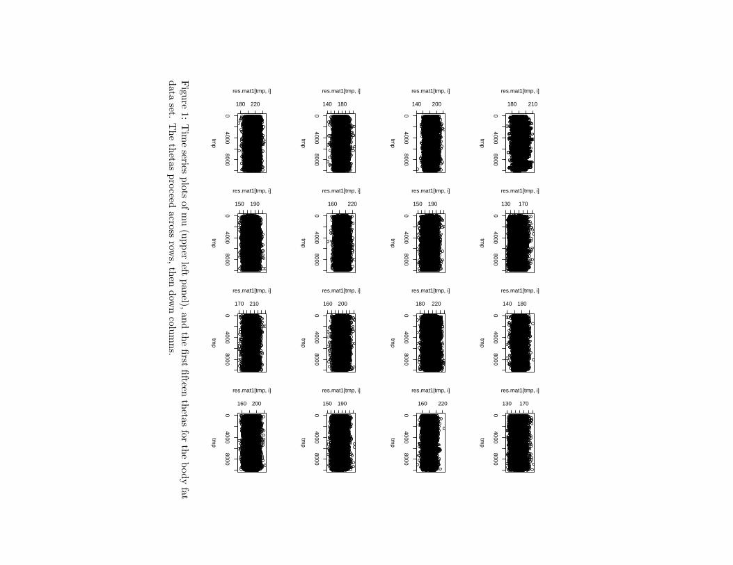
Figu
re1:
Tim
eseries
plots
ofm
u(u
pper
leftpan
el),an
dth
efirst
fifteen
thetas
forth
ebody
fatdata
set.T
he
thetas
pro
ceedacross
rows,
then
dow
ncolu
mns.
0 2000 4000 6000 8000 10000
4060
8010
0
tmp
tmp.
vec
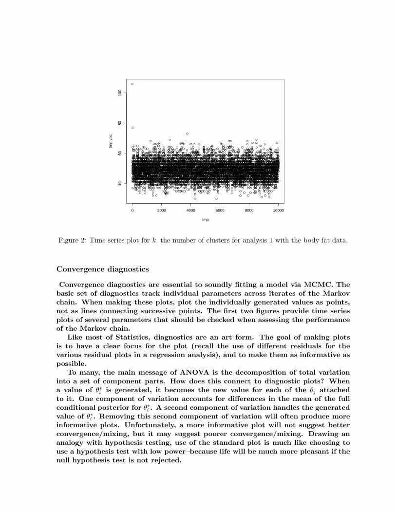
Figure 2: Time series plot for k, the number of clusters for analysis 1 with the body fat data.
Convergence diagnostics
Convergence diagnostics are essential to soundly fitting a model via MCMC. Thebasic set of diagnostics track individual parameters across iterates of the Markovchain. When making these plots, plot the individually generated values as points,not as lines connecting successive points. The first two figures provide time seriesplots of several parameters that should be checked when assessing the performanceof the Markov chain.
Like most of Statistics, diagnostics are an art form. The goal of making plotsis to have a clear focus for the plot (recall the use of different residuals for thevarious residual plots in a regression analysis), and to make them as informative aspossible.
To many, the main message of ANOVA is the decomposition of total variationinto a set of component parts. How does this connect to diagnostic plots? Whena value of θ∗i is generated, it becomes the new value for each of the θj attachedto it. One component of variation accounts for differences in the mean of the fullconditional posterior for θ∗i . A second component of variation handles the generatedvalue of θ∗i . Removing this second component of variation will often produce moreinformative plots. Unfortunately, a more informative plot will not suggest betterconvergence/mixing, but it may suggest poorer convergence/mixing. Drawing ananalogy with hypothesis testing, use of the standard plot is much like choosing touse a hypothesis test with low power–because life will be much more pleasant if thenull hypothesis test is not rejected.
150 200 250 300 350
150
200
250
300
data1$x
thet
a.ha
t1[2
:253
]
200 250 300
180
220
260
300
data2$x
thet
a.ha
t2[2
:113
]
150 200 250 300 350
150
200
250
300
data3$x
thet
a.ha
t3[2
:253
]
200 250 300
180
220
260
300
data4$x
thet
a.ha
t4[2
:113
]
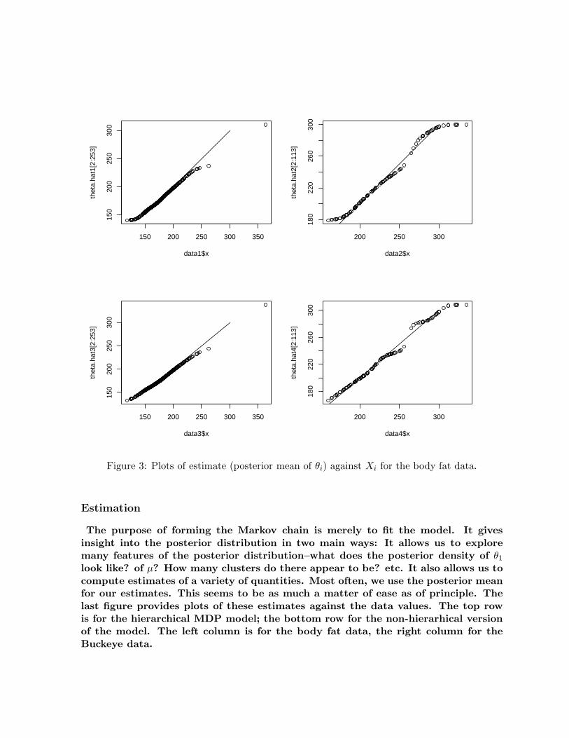
Figure 3: Plots of estimate (posterior mean of θi) against Xi for the body fat data.
Estimation
The purpose of forming the Markov chain is merely to fit the model. It givesinsight into the posterior distribution in two main ways: It allows us to exploremany features of the posterior distribution–what does the posterior density of θ1
look like? of µ? How many clusters do there appear to be? etc. It also allows us tocompute estimates of a variety of quantities. Most often, we use the posterior meanfor our estimates. This seems to be as much a matter of ease as of principle. Thelast figure provides plots of these estimates against the data values. The top rowis for the hierarchical MDP model; the bottom row for the non-hierarhical versionof the model. The left column is for the body fat data, the right column for theBuckeye data.