GGGG TTTTHESIS AAAA---2016.161 FDS ----222----Abaqus · AAAAUTHOR Name J.A. (Jelmer) Feenstra...
205
GRADUATION RADUATION RADUATION RADUATION THESIS HESIS HESIS HESIS A- 2016.161 2016.161 2016.161 2016.161 FDS FDS FDS FDS- 2- Abaqus Abaqus Abaqus Abaqus C++ C++ C++ C++ MANAGED AUTOMATED PY MANAGED AUTOMATED PY MANAGED AUTOMATED PY MANAGED AUTOMATED PYTHON SCRIPTED THON SCRIPTED THON SCRIPTED THON SCRIPTED CFD CFD CFD CFD- FEM FEM FEM FEM COUPLING COUPLING COUPLING COUPLING Additionally assessing two Additionally assessing two Additionally assessing two Additionally assessing two- - - way coupling effectiveness way coupling effectiveness way coupling effectiveness way coupling effectiveness J.A.Feenstra 0726615 August 2016
Transcript of GGGG TTTTHESIS AAAA---2016.161 FDS ----222----Abaqus · AAAAUTHOR Name J.A. (Jelmer) Feenstra...
GGGGRADUATIONRADUATIONRADUATIONRADUATION TTTTHESISHESISHESISHESIS AAAA----2016.1612016.1612016.1612016.161
FDSFDSFDSFDS----2222----AbaqusAbaqusAbaqusAbaqus
C++C++C++C++ MANAGED AUTOMATED PYMANAGED AUTOMATED PYMANAGED AUTOMATED PYMANAGED AUTOMATED PYTHON SCRIPTED THON SCRIPTED THON SCRIPTED THON SCRIPTED CFDCFDCFDCFD----FEMFEMFEMFEM COUPLINGCOUPLINGCOUPLINGCOUPLING
Additionally assessing twoAdditionally assessing twoAdditionally assessing twoAdditionally assessing two----way coupling effectivenessway coupling effectivenessway coupling effectivenessway coupling effectiveness
J.A.Feenstra
0726615
August 2016

FDS-2-ABAQUS: C++ MANAGED AUTOMATED PYTHON SCRIPTED CFD-FEM COUPLING
J.A. FEENSTRA I
Master Thesis of J.A.Feenstra for the degree of Master of Science to be submitted to the
Department of the Built Environment at Eindhoven University of Technology.
PPPPUBLICATIONUBLICATIONUBLICATIONUBLICATION
Project MSc. Thesis
Archive Code A-2016.161
Title FDS-2-Abaqus, C++ managed automated python scripted CFD-FEM coupling.
Additionally assessing two-way coupling effectiveness
Version 1.4 (Final)
Date August 2016
AAAAUTHORUTHORUTHORUTHOR
Name J.A. (Jelmer) Feenstra Student Number 0726615 Address Salamancapad 267
3584DX Utrecht Mobile Number +31 6 16 70 63 38 Mail address [email protected] EEEEINDHOVEN INDHOVEN INDHOVEN INDHOVEN UUUUNIVERSITY NIVERSITY NIVERSITY NIVERSITY OOOOF F F F TTTTECHNOLOGYECHNOLOGYECHNOLOGYECHNOLOGY
Faculty Department of the Built Environment Master Architecture Building and Planning Master Track Structural Design Chair Applied Mechanics GGGGRADUATION COMMITTEERADUATION COMMITTEERADUATION COMMITTEERADUATION COMMITTEE
Chairman dr. ir. H. Hofmeyer [TU/e – Netherlands] 2nd member prof. M. Mahendran [QUT – Australia] 3rd member ir. R.A.P. van Herpen [TU/e – Netherlands]

II MASTER THESIS

FDS-2-ABAQUS: C++ MANAGED AUTOMATED PYTHON SCRIPTED CFD-FEM COUPLING
J.A. FEENSTRA III
PREFACE
Before you lies my graduation thesis for my master Structural Design at Eindhoven University of
Technology. Within this thesis a program called FDS-2-Abaqus was developed which can be used to
perform one and two-way coupled CFD-FEM analyses. FDS-2-Abaqus was used to study the
feasibility and effectiveness of a two-way coupled of CFD-FEM analysis.
In the past year I was able to develop numerous skills. Most notably my ability to read and write code.
The core process of coding is to continuously subdivide a problem until you can solve one with a simple
line of code. I think this process is widely applicable in any project. Looking back there are numerous
things that I, in retrospect, would like to do or approach differently. Actually illustrating the numerous
skills I developed over the course of this project.
This thesis would not have been a success without the support and encouragement of my environment.
Therefore I would like to thank my supervisors for their guidance throughout this project. I am very
grateful for their encouragement, explanations, and enthusiasm. It helped me keep motivated and were
vital to the successful completion of this project. Thank you Herm Hofmeyer for our in depth discussion
in which we always seemed to run out of time. Thank you Ruud van Herpen for your clear explanations
on fire. Also thanks to prof. Mahen Mahendran of Queensland University of Technology for his interest
in my project and his feedback on my writing.
In addition I would like to thank my family and friends for their support and interest throughout this
project. You guys really never seemed bored. A special shout out to my parents who have always
encouraged and supported me.
Jelmer Auke Feenstra
Utrecht, August 2016


FDS-2-ABAQUS: C++ MANAGED AUTOMATED PYTHON SCRIPTED CFD-FEM COUPLING
J.A. FEENSTRA V
ABSTRACT
Coupling of CFD fire simulations to thermo-mechanical FE models is a relative new area of research. A
distinction is made between one and two way coupling where in a two way coupled analysis the effect
of the structural response on the fire propagation is taken into account. The effect of mechanical
behaviour on the fire has only been studied in a very limited number of cases.
The aim of this thesis is to study the feasibility of the two-way coupling of CFD fire simulations to FE
heat transfer and structural response analyses. More specifically to compare the difference in failure
propagation of a thin walled steel façade subjected to fire for a one and two-way coupled analysis.
Coupled CFD-FEM fire to thermomechanical analysis can be split into three separate types of analysis
(a1) fire simulations, (a2) heat transfer analysis, and (a3) structural response analysis. These Analysis
steps and their mutual coupling steps, have been studied separately. For the fire simulation the CFD
software Fire Dynamic Simulator (FDS) by NIST is used. Both the heat transfer (HT) and the structural
response (SR) analyses are modelled using FE software Abaqus.
FDS-2-Abaqus is a managing program developed during this thesis to facilitate the one and two-way
coupling of a CFD-FEM analysis. FDS-2-Abaqus was used to perform one and two way coupled
analyses of an office space comprising a twelve plate thin walled steel façade. The results were used
to assess the effectiveness of two-way coupling. Concluding that the significant difference in failure
progression illustrates both the feasibility and the effectiveness of two-way coupling. Although
additional research, using more advanced fire and structural models, is required for an all conclusive
answer.

FDS-2-ABAQUS: C++ MANAGED AUTOMATED PYTHON SCRIPTED CFD-FEM COUPLING
J.A. FEENSTRA VII
ABBREVIATIONS AND SYMBOLS
Overview of abbreviations and symbols used throughout this thesis.
ABBREVIATIONS
ASTASTASTAST Adiabatic Surface Temperature
CFDCFDCFDCFD Computational Fluid Dynamics
DOFDOFDOFDOF Degree of Freedom
FDSFDSFDSFDS Fire Dynamic Simulator
FEAFEAFEAFEA Finite Element Analysis
FEMFEMFEMFEM Finite Element Method
HRRHRRHRRHRR Heat Release Rate
HTHTHTHT Heat Transfer
OWCOWCOWCOWC One-Way Coupled / One-Way Coupling
SRSRSRSR Structural Response
TWCTWCTWCTWC Two-Way Coupled / Two-Way Coupling
SYMBOLS - GREEK
α Coefficient of thermal expansion -1[K ]
ε Emissivity -
longε Longitudinal strain -
transε Transverse strain -
ν Poisson’s ratio -
thσ Thermal Stress -2[N m ]⋅
boltzσ Stefan Boltzmann Constant 8 -2 -45,5703 10 [W m K ]−
⋅ ⋅
SYMBOLS – LATIN
fiA Total fire surface
2[m ]
htA Heat transfer surface 2[m ]
c Specific heat -1 -1[J kg K ]⋅
E Young’s modulus -2[N m ]⋅
F View factor -
fHRR Heat release rate
-2[W m ]⋅
ch Convective heat transfer coefficient -2 -1[W m K ]⋅
k Thermal conductivity -2 -1[W m K ]⋅
L∆ Elongation [m]
0L Original length [m]
m Unit mass [kg]
Q Thermal energy [J]
fiQ Net heat of combustion [J]

VIII MASTER THESIS
q Heat rate [W]
q„ Heat flux
2[W m ]−⋅
cdq Conductive heat rate [W]
cvq Conductive heat rate [W]
fiq Fire load density
2[J m ]−⋅
radq Radiative heat rate [W]
incq„ Incident radiation flux
2[W m ]−⋅
ambT Absolute ambient temperature [K]
ASTT Adiabatic Surface Temperature [K]
gasT Absolute temperature of fluid [K]
surfT Absolute surface temperature [K]
t Duration [s]
0t Duration flashover phase [s]
1t Duration fully-developed phase [s]
2t Duration decay phase [s]
fit Total fire duration [s]

FDS-2-ABAQUS: C++ MANAGED AUTOMATED PYTHON SCRIPTED CFD-FEM COUPLING
J.A. FEENSTRA 1
TTTTABLE OF ABLE OF ABLE OF ABLE OF CCCCONTENTSONTENTSONTENTSONTENTS
Preface .................................................................................................................................................... III
Abstract ................................................................................................................................................... V
Abbreviations and Symbols ................................................................................................................... VII
1. Introduction ...................................................................................................................................... 3
2. Theory .............................................................................................................................................. 5
2.1 Coupling of Fire Simulations and Structural Analysis .............................................................. 5
2.2 Fire ........................................................................................................................................... 6
2.3 Fire Load and Heat Release Rate ............................................................................................ 8
2.4 Heat Transfer ......................................................................................................................... 10
2.5 Adiabatic Surface Temperature ............................................................................................. 14
3. Approach ........................................................................................................................................ 17
4. Experimental Setup: Model Room ................................................................................................. 21
4.1 Design .................................................................................................................................... 21
4.2 Thin Walled Steel Façade Systems ....................................................................................... 22
4.3 Fire Scenario .......................................................................................................................... 23
5. Simulating Fire with Fire Dynamic Simulator ................................................................................. 25
5.1 Fire Dynamic Simulator (FDS) ................................................................................................ 25
5.2 Writing an FDS Input FIle ...................................................................................................... 26
5.3 Modifying the Fire Model During Simulation ......................................................................... 31
6. Abaqus Analysis ............................................................................................................................. 35
6.1 Abaqus CAE ........................................................................................................................... 35
6.2 Basic Model ........................................................................................................................... 36
6.3 Heat Transfer Analysis ........................................................................................................... 38
6.4 Structural Response Analysis ................................................................................................ 41
6.5 Multiple Plate Models ............................................................................................................ 45
6.6 Restart Analysis ..................................................................................................................... 46
6.7 Removing Plates .................................................................................................................... 47
7. Programs and Scripts ..................................................................................................................... 49
7.1 Coupling Methodology .......................................................................................................... 49
7.2 FDS-2-Abaqus ........................................................................................................................ 51
7.3 reWriteAST2py ...................................................................................................................... 54
7.4 upGeomFDS .......................................................................................................................... 56
7.5 upGeomHT ............................................................................................................................ 57
7.6 upGeomSR ............................................................................................................................ 59
7.7 PlateFailureCheck.py ............................................................................................................. 61
ADDITIONALLY ASSESSING TWO-WAY COUPLING EFFECTIVENESS
2 MASTER THESIS
8. Results and Discussion .................................................................................................................. 65
8.1 Effectiveness Study: Twelve Plates ...................................................................................... 65
8.2 Tied Multi Plate Models ......................................................................................................... 69
9. Conclusions and Recommendations .............................................................................................. 73
9.1 Conclusions ........................................................................................................................... 73
9.2 Recommendations for Future Research ............................................................................... 74
References ............................................................................................................................................ 77
FDS-2-ABAQUS: C++ MANAGED AUTOMATED PYTHON SCRIPTED CFD-FEM COUPLING
J.A. FEENSTRA 3
1. INTRODUCTION
The traditional approach of structural response to fire is by imposing prescriptive time temperature
curves on the structure. This approach is widely used in standards and codes, for example the ISO
cellulosic fire curve included in EC1 1-2 [1]. Fire safety design thereby revolves around meeting fire
resistance times for the separate structural components. Advanced numerical models based on the
Finite Element Method (FEM) are used nowadays to predict local and global structural behaviour. In
addition these methods have been applied to predict structural response to fire. However the use of
the simplified time-temperature curves do not take into account the randomness of fire and therefore
cannot accurately represent the fire. Fire evolution is governed by fuel distribution, oxygen supply, and
the geometric boundary conditions of the compartment. More advanced numerical models based on
Computational Fluid Dynamics (CFD) are capable of modelling the three dimensional fire propagation
more accurately.
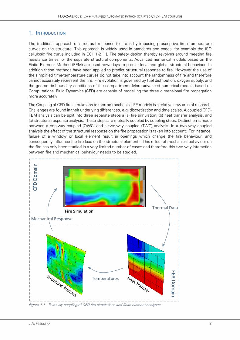
The Coupling of CFD fire simulations to thermo-mechanical FE models is a relative new area of research.
Challenges are found in their underlying differences, e.g. discretization and time scales. A coupled CFD-
FEM analysis can be split into three separate steps a (a) fire simulation, (b) heat transfer analysis, and
(c) structural response analysis. These steps are mutually coupled by coupling steps. Distinction is made
between a one-way coupled (OWC) and a two-way coupled (TWC) analysis. In a two way coupled
analysis the effect of the structural response on the fire propagation is taken into account. For instance,
failure of a window or local element result in openings which change the fire behaviour, and
consequently influence the fire load on the structural elements. This effect of mechanical behaviour on
the fire has only been studied in a very limited number of cases and therefore this two-way interaction
between fire and mechanical behaviour needs to be studied.
CF
D D
om
ain
FE
A D
om
ain
Temperatures
Thermal Data
Mechanical Response
Fire Simulation
Figure 1.1 - Two way coupling of CFD fire simulations and finite element analyses
ADDITIONALLY ASSESSING TWO-WAY COUPLING EFFECTIVENESS
4 MASTER THESIS
The aim of this thesis is to study the feasibility of the two-way coupling of CFD fire simulations to FE
heat transfer and structural response analyses, as illustrated in Figure 1.1. Several programs and scripts
were developed to facilitate and automate both one- and two-way CFD-FEM coupling. The developed
managing program FDS-2-Abaqus was used to perform one and two way coupled analyses on an
office space comprising a twelve plate thin walled steel façade. The results were used to assess the
effectiveness of two-way coupling.
This thesis is structured as follows. Chapter 2 contains a selection of relevant literature topics where,
among others, heat transfer is discussed. Chapter 3 discusses the approach to the coupling, the
methodology. A model room, and fire scenario, to act as a starting point for the coupling procedure is
developed in chapter 4. Chapter 5 discusses fire simulation using the software Fire Dynamic Simulater
(FDS) by NIST. The subsequent thermal and structural response analysis are performed using finite
element software Abaqus, and discussed in chapter 6. The development of the various coupling
programs and scripts are discussed chapter 7. The assessment on the effectiveness of two way
coupling is presented as part of the results in chapter 8. Lastly, the conclusions and recommendations
are presented in chapter 9.
RESEARCH QUESTIONS
The main question for this thesis is presented below:
“Is the two-way coupling of CFD fire simulations to finite heat transfer and structural response
analysis a feasible technique for use in structural fire safety design?”
This main question has been elaborated in various sub questions as follows:
“How does a two-way coupling perform compared to a one-way coupled CFD-FEM? “
“What separate analysis steps can be identified and how to perform and implement these in a
coupled analysis?”
“What coupling steps can be identified and what data exchange occurs between the analysis
steps?”
“What tools are required to facilitate and automate the coupling procedure?”
In a sense these questions loosely translate to a can, how and should question. Can we do it? Should
we do it? And How to do it? The questions have been answered throughout this report by first
investigating the separate analyses and coupling steps. Subsequently programs and scripts have been
developed to facilitate one and two way CFD-FEM coupling.
SOCIAL RELEVANCE
The thesis focusses on the feasibility of coupling fire simulation to finite element analysis. In a sense
this is very specific, but in the long run it could contribute to a better understanding of fire and its
behaviour. Fire often results in the loss of human life. Therefore, understanding fire and its effects
could contribute to fire safety and structural performance. In addition it is important to note that the
majority of the victims of an earthquake are due to resulting fires in the aftermath of the earthquake.
Again underlining the importance of fire safety. This research could also be relevant to the field of
engineering. Large projects often take advantage of BIM models. BIM models incorporate aspects of
all different professions into one big model. This study could contribute to such models by integrating
fire analyses with structural analyses possibly resulting in more efficient and safe solutions.
FDS-2-ABAQUS: C++ MANAGED AUTOMATED PYTHON SCRIPTED CFD-FEM COUPLING
J.A. FEENSTRA 5
2. THEORY
Several relevant topics to this research are explained. First the coupling of fire simulations to structural
analysis is explored. Followed by fire, fire load, heat transfer and the concept of adiabatic surface
temperature.
2.1 COUPLING OF FIRE SIMULATIONS AND STRUCTURAL ANALYSIS
Coupling of CFD fire simulations and structural finite element analyses is a relatively new area of
research. One of the reasons for the resurgence of interest in thermo-mechanical response to fire was
due to the attacks on the World Trade Centre (WTC) towers in 2001. In the aftermath of the collapse
Prasad and Baum (2005) [2] developed an interface model to couple the gas phase energy release and
fluid movements with the stress analysis in the load bearing materials. Their procedure, used in the
analysis of the collapse of the WTC towers, couples CFD with FEA based on heat transfer by radiation
and conduction. The resulting method, called Fire Structural Interface (FSI) can be used to generate
realistic thermal boundary conditions for use in solutions to the heating of complex structures. Later
work by Baum (2011) [3] discusses the fire-thermomechanical coupling. Specifically it discusses the
role of uncertainty in input parameters and provides a context to illustrate the strengths and
weaknesses of employed coupling methodologies.
The European research project FIRESTRUC analysed coupling methodologies for predicting thermo-
mechanical behaviour. The FIRESTRUC paper by Welch et al (2006) [4] shows a broad examination of
approaches to coupling CFD and FEM codes, while taking into account the implications for accuracy
and computational requirements. Each of the analysis and coupling steps are discussed separately in
the paper and multiple methods are proposed for both one and two-way coupling.
Luo et al. [5] developed an Fire Interface Simulator Toolkit (AFIST) by integrating CFD software Fire
Dynamic Simulator (FDS) with a customized Abaqus structural analyser through a two-way coupling. A
two-way coupling exchange of heat and mass flow is integrated on the incremental level. In addition
various demonstration and validation methods are presented to illustrate the capability of the tool.
The concept of adiabatic surface temperature (AST) was introduced by Wickström et al. in 2007 [6].
Adiabatic surface temperature is a practical tool to express the thermal exposure of a surface to fire in
a single quantity, thereby reducing the data flow. The AST concept and associated equations are
discussed in more detail in paragraph 2.5. Duthinh et al (2008) [7] utilized AST to developed an interface
between fire simulation software FDS and FEA software ANSYS. They applied their interface to a
trussed beam and verified it using a real life fire test by NIST. Another example of utilizing AST to couple
CFD and FEA analyses is found in a paper by Banerjee et al (2009) [8]. Banerjee et al. created an
Immersive Visualization Environment (IVE) to visualize, and study, in real time the structural and thermal
behaviour of a chosen structural element under fire. For the initial study a beam was selected as
structural element. The software Fire Dynamic Simulator (FDS) was used to simulate the onset and
development of fire in a typical room. Subsequently the resulting gas temperatures were imposed on
a simulated beam using finite element software Abaqus. Finally Abaqus was used to compute the
deformation over time as a result of the thermal and mechanical loads.
Silva et al (2014) [9] developed a computational interface model, the Fire- Thermomechanical Interface
(FTMI), to provide an interface for fire-thermomechanical performance based analysis of structures
under fire. The interface allows for coupling of the fire-driven fluid model FDS and structural
thermomechanical analysis via ANSYS. The coupling allows for both convective and radiative heat
transfer to the exposed surface by utilizing the AST concept. In the paper the methodology is described
and applied to a simple case for verification. In addition the code has been added to the FDS repository
under the name FDS2FTMI allowing for one-way coupling of FDS and finite element software ANSYS
[10]. Additional validation of FDS2FTMI was carried out by Zhang et al (2015) [11].

ADDITIONALLY ASSESSING TWO-WAY COUPLING EFFECTIVENESS
6 MASTER THESIS
The transfer of data between analysis models can get rather complicated because of difference in
discretization and time scale. Banerjee (2014) [12] discusses software independent mapping tools to
assist in both types of data transfer for one-way coupling. More specifically, the transfer from fire model
to heat transfer model, and subsequently from the heat transfer model to the structural analysis model.
2.2 FIRE
According to the encyclopedia of Natural Hazards
fire can be defined as the combustion (a series of
chemical reactions) between a fuel (an organic
compound) and an oxidant (oxygen source)
producing heat, light, and often sound [13].
Chemically speaking is fire a rapid exothermic
oxidation of a combustible material accompanied by
the evolution of heated gaseous products of
combustion. The previous description hint at the
conditions needed for the onset, and continuation
of fire. The requirements for fire are oxygen, fuel,
heat, and chemical chain reaction. The first three
elements are required to trigger the fire. The
oxidizing agent (oxygen) sustains combustion, heat
is needed to raise the material to its ignition
temperature, and a combustible material (fuel) acts
as the reducing agent. Once triggered the fire is sustained by a chemical chain reaction and keeps
burning until one of the conditions is removed or blocked. These requirements are commonly
symbolized by the fire tetrahedron (or triangle, excluding the chain reaction) as shown in Figure 2.1.
STAGES OF A FIRE
Both the trigger and development of a compartment fire are random and vary greatly for specific
situations. Despite this randomness a general behaviour can be explained and understood. Given a
compartment fire four stages can be recognized: the initial, flashover, fully developed, and cooling
phase. These stages are illustrated in Figure 2.2 and discussed in more detail below.
Figure 2.2 - The four stages in a compartment fire [14]
Initial Stage of the Fire
The first stage of the fire, also called incipient, is characterized by ignition. Heat, fuel and oxygen
combine and form a chemical chain reaction resulting in a fire. During this stage the fire is fuel
controlled, there is sufficient oxygen for all (currently burning) fuel to combust. Once triggered the
gaseous products, generated by the fire, form a hot layer of gases close to the ceiling. The fire gradually
Figure 2.1 - The Fire Tetrahedron
FDS-2-ABAQUS: C++ MANAGED AUTOMATED PYTHON SCRIPTED CFD-FEM COUPLING
J.A. FEENSTRA 7
heats its surroundings due to the overall temperature increase from the continuing generating of heated
gases. The increase in temperature combined with the availability of both oxygen and fuel will cause
the fire to grow in size at an increasing rate [14], [15].
.
Flashover
With the growth of the fire the temperatures of its surroundings keep increasing. The fire can develop
to such an extent that the compartment and its interior can reach a certain temperature that allows for
flashover to occur. Flashover is a rapid transition resulting in total surface involvement of all combustible
materials in the compartment. In other words all combustible material reach their ignition temperature
resulting in a fully developed fire. However, this can only occur when sufficient oxygen is available, if
oxygen is limited the fire’s intensity will decrease which results in the fire burning out or devolve into a
smouldering fire. Generally flashover occurs at temperatures ranging from 600 - 700 °C [14], [15].
Fully Developed
After flashover the fire is fully developed when all combustible material is ignited. Flames rush out
through openings and the heat of the surrounding structures greatly increases. This poses a great threat
for spreading to adjoining rooms or buildings. The heat release is at its greatest, although limited by
ventilation (availability of oxygen). The average gas temperatures within the compartment range from
700 - 1200 °C [14], [15].
Cooling Phase
The cooling phase is initiated as a result of limited availability of fuel or oxygen, in the end resulting in
the end of the fire. Simply put, the cooling phase is the dying out of the fire due to lack of resources.
When insufficient oxygen is available the end stage results in hot pyrolized fuel and flammable gaseous
products of combustion. These products present a threat since they could re-ignite when introduced to
a source of oxygen, so called backdraft. Backdraft is the burning of heated gaseous products of
combustion when oxygen is introduced into an environment that has a depleted supply of oxygen due
to fire. This burning often occurs with explosive force [14], [15].
ADDITIONALLY ASSESSING TWO-WAY COUPLING EFFECTIVENESS
8 MASTER THESIS
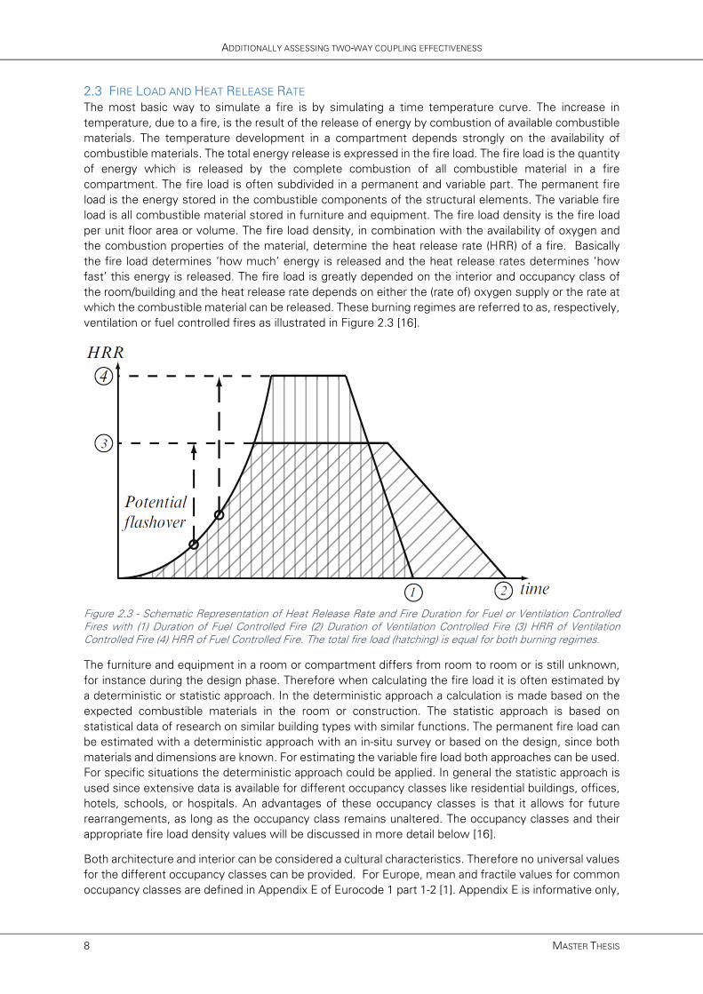
2.3 FIRE LOAD AND HEAT RELEASE RATE
The most basic way to simulate a fire is by simulating a time temperature curve. The increase in
temperature, due to a fire, is the result of the release of energy by combustion of available combustible
materials. The temperature development in a compartment depends strongly on the availability of
combustible materials. The total energy release is expressed in the fire load. The fire load is the quantity
of energy which is released by the complete combustion of all combustible material in a fire
compartment. The fire load is often subdivided in a permanent and variable part. The permanent fire
load is the energy stored in the combustible components of the structural elements. The variable fire
load is all combustible material stored in furniture and equipment. The fire load density is the fire load
per unit floor area or volume. The fire load density, in combination with the availability of oxygen and
the combustion properties of the material, determine the heat release rate (HRR) of a fire. Basically
the fire load determines ‘how much’ energy is released and the heat release rates determines ‘how
fast’ this energy is released. The fire load is greatly depended on the interior and occupancy class of
the room/building and the heat release rate depends on either the (rate of) oxygen supply or the rate at
which the combustible material can be released. These burning regimes are referred to as, respectively,
ventilation or fuel controlled fires as illustrated in Figure 2.3 [16].
Figure 2.3 - Schematic Representation of Heat Release Rate and Fire Duration for Fuel or Ventilation Controlled Fires with (1) Duration of Fuel Controlled Fire (2) Duration of Ventilation Controlled Fire (3) HRR of Ventilation Controlled Fire (4) HRR of Fuel Controlled Fire. The total fire load (hatching) is equal for both burning regimes.
The furniture and equipment in a room or compartment differs from room to room or is still unknown,
for instance during the design phase. Therefore when calculating the fire load it is often estimated by
a deterministic or statistic approach. In the deterministic approach a calculation is made based on the
expected combustible materials in the room or construction. The statistic approach is based on
statistical data of research on similar building types with similar functions. The permanent fire load can
be estimated with a deterministic approach with an in-situ survey or based on the design, since both
materials and dimensions are known. For estimating the variable fire load both approaches can be used.
For specific situations the deterministic approach could be applied. In general the statistic approach is
used since extensive data is available for different occupancy classes like residential buildings, offices,
hotels, schools, or hospitals. An advantages of these occupancy classes is that it allows for future
rearrangements, as long as the occupancy class remains unaltered. The occupancy classes and their
appropriate fire load density values will be discussed in more detail below [16].
Both architecture and interior can be considered a cultural characteristics. Therefore no universal values
for the different occupancy classes can be provided. For Europe, mean and fractile values for common
occupancy classes are defined in Appendix E of Eurocode 1 part 1-2 [1]. Appendix E is informative only,
FDS-2-ABAQUS: C++ MANAGED AUTOMATED PYTHON SCRIPTED CFD-FEM COUPLING
J.A. FEENSTRA 9
meaning national Appendixes are allowed to define different values. Outside of Europe, the
International Fire Engineering Guidelines (IFEG) [17] are considered for information concerning fire load
densities for both specific and common occupancy classes. Both standards refer to the CIB W14, an
international overview on fire load surveys conducted before 1986. It is important to note that the
present-day furnishing and construction materials are different from what was customary several
decades ago. A more recent overview on fire load densities in office buildings is found in a paper by
Khorasani et al. (2013) [18]. The paper discusses that recent surveys indicate a large range of fire load
density values, and show strong correlation between fire load density, compartment area, and use.
These variables are not account for in current codes (like Eurocode). Showing, for instance, that
Eurocode is conservative for ‘lightweight’ (general, clerical, lobby, and conference) and non-
conservative on ‘heavyweight’ (file, storage, and library) compartment use. In addition new fire load
density and maximum temperature models are proposed by Khorasani et al. for application in
probabilistic performance-based fire design, taking into consideration the area and compartment use.
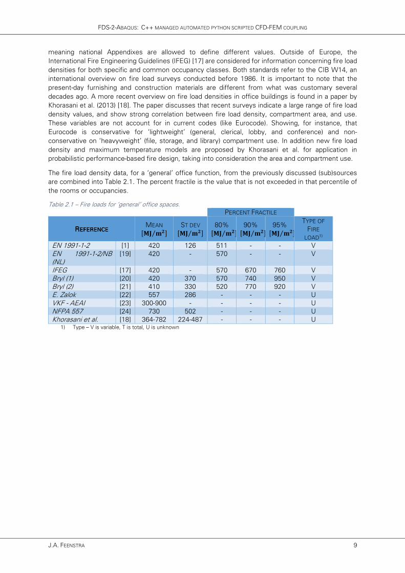
The fire load density data, for a ‘general’ office function, from the previously discussed (sub)sources
are combined into Table 2.1. The percent fractile is the value that is not exceeded in that percentile of
the rooms or occupancies.
Table 2.1 – Fire loads for ‘general’ office spaces.
PERCENT FRACTILE
RRRREFERENCEEFERENCEEFERENCEEFERENCE MEAN
��� ��⁄ �
ST DEV
��� ��⁄ �
80%
��� ��⁄ �
90%
��� ��⁄ �
95%
��� ��⁄ �
TYPE OF
FIRE
LOAD1)
EN 1991-1-2 [1] 420 126 511 - - V
EN 1991-1-2/NB (NL)
[19] 420 - 570 - - V
IFEG [17] 420 - 570 670 760 V
Bryl (1) [20] 420 370 570 740 950 V
Bryl (2) [21] 410 330 520 770 920 V
E. Zalok [22] 557 286 - - - U
VKF - AEAI [23] 300-900 - - - - U
NFPA 557 [24] 730 502 - - - U
Khorasani et al. [18] 364-782 224-487 - - - U 1) Type – V is variable, T is total, U is unknown
ADDITIONALLY ASSESSING TWO-WAY COUPLING EFFECTIVENESS
10 MASTER THESIS
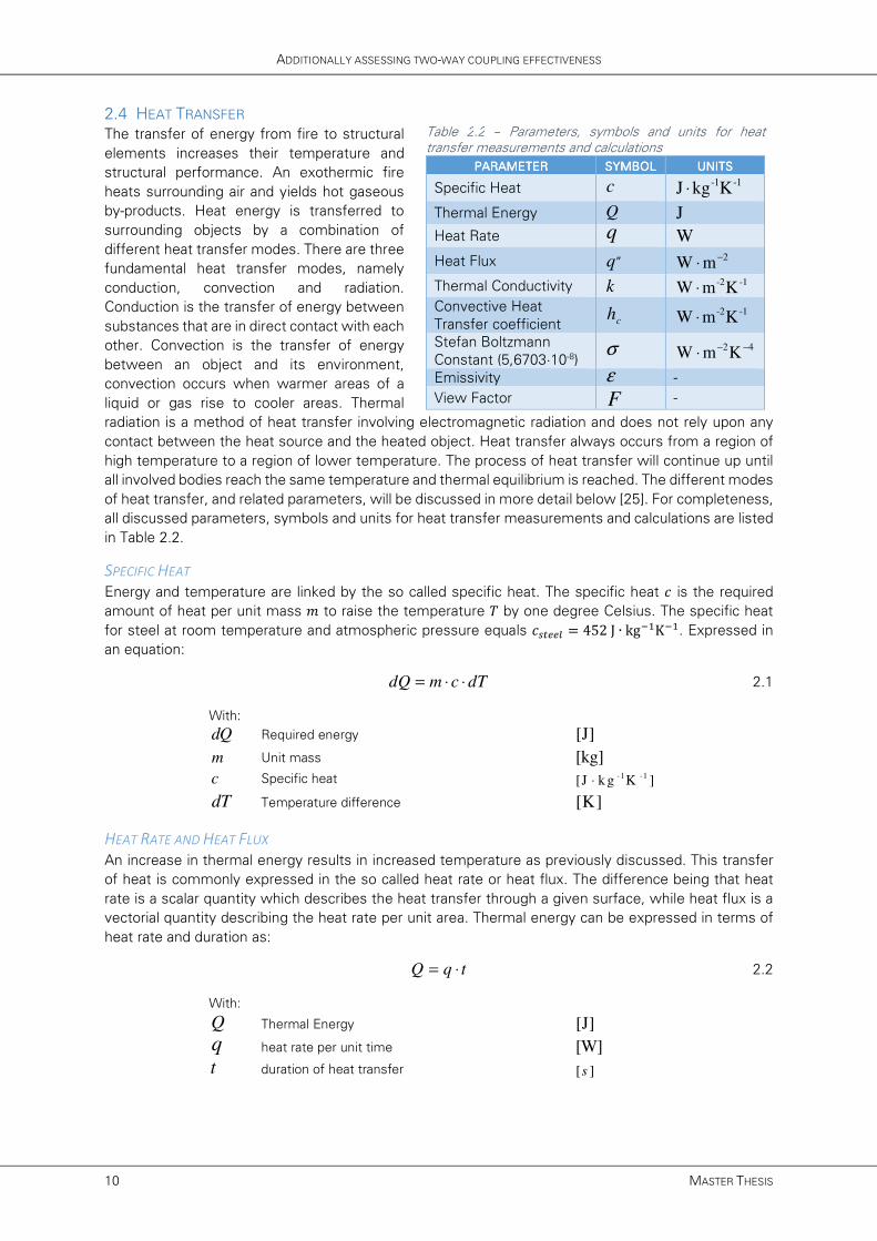
2.4 HEAT TRANSFER
The transfer of energy from fire to structural
elements increases their temperature and
structural performance. An exothermic fire
heats surrounding air and yields hot gaseous
by-products. Heat energy is transferred to
surrounding objects by a combination of
different heat transfer modes. There are three
fundamental heat transfer modes, namely
conduction, convection and radiation.
Conduction is the transfer of energy between
substances that are in direct contact with each
other. Convection is the transfer of energy
between an object and its environment,
convection occurs when warmer areas of a
liquid or gas rise to cooler areas. Thermal
radiation is a method of heat transfer involving electromagnetic radiation and does not rely upon any
contact between the heat source and the heated object. Heat transfer always occurs from a region of
high temperature to a region of lower temperature. The process of heat transfer will continue up until
all involved bodies reach the same temperature and thermal equilibrium is reached. The different modes
of heat transfer, and related parameters, will be discussed in more detail below [25]. For completeness,
all discussed parameters, symbols and units for heat transfer measurements and calculations are listed
in Table 2.2.
SPECIFIC HEAT
Energy and temperature are linked by the so called specific heat. The specific heat is the required
amount of heat per unit mass to raise the temperature � by one degree Celsius. The specific heat
for steel at room temperature and atmospheric pressure equals � ��� = 452 J ∙ kg��K��. Expressed in
an equation:
dQ m c dT= ⋅ ⋅ 2.1
With:
dQ Required energy [J]
m Unit mass [kg]
c Specific heat -1 -1[J k g K ]⋅
dT Temperature difference [K]
HEAT RATE AND HEAT FLUX
An increase in thermal energy results in increased temperature as previously discussed. This transfer
of heat is commonly expressed in the so called heat rate or heat flux. The difference being that heat
rate is a scalar quantity which describes the heat transfer through a given surface, while heat flux is a
vectorial quantity describing the heat rate per unit area. Thermal energy can be expressed in terms of
heat rate and duration as:
Q q t= ⋅ 2.2
With:
Q Thermal Energy [J]
q heat rate per unit time [W]
t duration of heat transfer [ ]s
Table 2.2 – Parameters, symbols and units for heat transfer measurements and calculations
PARAMETERPARAMETERPARAMETERPARAMETER SYMBOLSYMBOLSYMBOLSYMBOL UNITSUNITSUNITSUNITS
Specific Heat c -1 -1J kg K⋅
Thermal Energy Q J
Heat Rate q W
Heat Flux q„ 2W m−
⋅
Thermal Conductivity k -2 -1W m K⋅
Convective Heat
Transfer coefficient ch -2 -1W m K⋅
Stefan Boltzmann
Constant (5,6703∙10-8) σ 2 4W m K− −
⋅
Emissivity ε -
View Factor F -
FDS-2-ABAQUS: C++ MANAGED AUTOMATED PYTHON SCRIPTED CFD-FEM COUPLING
J.A. FEENSTRA 11
In turn, heat rate can be expressed in terms of heat flux and surface area.
ht
q q A= ⋅„
2.3
With:
htA Heat transfer area of the surface 2
[m ]
q„ Heat Flux 2[W m ]−
⋅
CONDUCTION
Conduction is the flow of heath through solids and liquids by vibration and collision of molecules. Heat
is transferred from high energetic to less energetic molecules through collision. Since high temperature
is associated with high molecular energy heat energy transfers in direction of the lower temperatures.
Conduction occurs if there is a temperature gradient within a solid or fluid medium.
Thermal conductivity � is the property of a material to conduct heat. The thermal conductivity for
(carbon) steel at room temperature equals � = 53,3 W ∙ m��K�� and drops linearly to � = 27,3 W ∙
m��K�� at � = 800 °C. The total conductive heat transfer to a surface can be expressed as:
cd ht
dTq k A
ds= ⋅ 2.4
With:
cdq Conductive heat transfer per unit time [W]
k Thermal conductivity -2 -1[W m K ]⋅
d T
d s Temperature gradient over distance s 1
[K m ]−
⋅
CONVECTION
Convection is the transfer of heat energy between a surface and a moving fluid (liquid or gas) at different
temperatures. A distinction is made between forced and natural convection. Forced convection, also
known as assisted convection, occurs when an external force induces a fluid flow. For instance a pump,
mixer or fan. Natural convection, also known as free convection, is caused by buoyant forces resulting
from density variations due to variations in temperature in the fluid. At the interface layer between fluid
and surface the hot fluid transfers heat and, as a result of its increase in density, sinks. Therefore this
cooled fluid is replaced by hot fluid, which in turn transfers heat, sinks, and is replaced by hot fluid. This
continuous process is known as natural or free convection [25].
Convective heat transfer depends on the area of the surface, the temperature difference, and the so
called convective heat transfer coefficient. The convective heat gain of a surface can be expresses as:
( )cv c ht gas surfq h A T T= ⋅ − 2.5
With:
cvq Convective heat transfer per unit time [W]
ch Convective heat transfer coefficient -2 -1[W m K ]⋅
gasT Temperature of fluid (gas) [K]
surfT Surface temperature [K]

ADDITIONALLY ASSESSING TWO-WAY COUPLING EFFECTIVENESS
12 MASTER THESIS
The convective heat transfer coefficient of air
depends on the relative speed of the surface
through the air and can be approximated using the
equation 2.6 or the graph in Figure 2.4. It is
important to note that it concerns an empirical
equation and can only be used for velocities from
2 < & ≤ 20 m ∙ s�� [25].
0,5
, 10.45 10c air
h v v= − + ⋅ 2.6
With:
ν The relative speed of the object through the air 1[m s ]
−⋅
RADIATION
Heat transfer through radiation is the increase in temperature due to absorbing electromagnetic waves.
Radiation heat transfer can be described by reference to a black body. A black body is an idealized
object that absorbs all electromagnetic radiation that falls on its surface. By absorbing this energy its
inner building blocks are agitated, resulting in an increased temperature of the object in comparison to
its surroundings. This heat is then emitted in the form of electromagnetic radiation. Theoretically a black
body will emit radiation on all wavelengths, although at low temperatures the amount of visible light is
negligible and the radiation mainly comprises infrared radiation. The emission spectrum of such a black
body was first fully described by Max Planck [25].
The radiation energy per unit time from a black body is proportional to the fourth power of the absolute
temperature and can be expressed with Stefan-Boltzmann Law as:
4
radq T Aσ= ⋅ ⋅ 2.7
With:
radq Radiative heat loss per unit time [W]
boltzσ Stefan Boltzmann Constant (5,6703∙10-8) 2 4[W m K ]
− −⋅
T Absolute temperature [K]
A Area of the emitting body 2[m ]
Since black bodies don’t exist in nature the
Stefan-Boltzmann Law for other objects, so called
‘grey bodies’, includes a factor ) describing the
emissivity of the object. The emissivity coefficient
) indicates the radiation of heat from a grey body
compared to the radiation of heat form an ideal
black body ) = 1,0. The emissivity depends on the
type of material and its surface finishing as
illustrated in Table 2.3 for steel [25]. In most cases
of structural materials being exposed to fire, it can
be assumed equal to 0.8 [6].
Figure 2.4 – Convective heat transfer coefficient (air)
Table 2.3 – Emissivity of steel
MMMMATERIALATERIALATERIALATERIAL EEEEMISSIVITY MISSIVITY MISSIVITY MISSIVITY +
Steel Oxidized 0,79
Steel Polished 0,07
Stainless Steel, weathered 0,85
Stainless Steel, polished 0,075
Steel Galvanized (Old) 0,88
Steel Galvanized (New) 0,23
0
10
20
30
40
00 05 10 15 20
hc,
air
[W∙m
-2KK KK-- -- 11 11
]
ν [m/s]

FDS-2-ABAQUS: C++ MANAGED AUTOMATED PYTHON SCRIPTED CFD-FEM COUPLING
J.A. FEENSTRA 13
4
radq Tε σ= ⋅ ⋅ 2.8
With:
ε Emissivity of the object [ ]−
Above formulation describes heat loss by radiation. The net radiation heat received by a surface is the
difference between the absorbed incident radiation and the radiation emitted from the surface. Both
heat transfer through the surface and the influence of various wavelengths are neglected. Resulting in
equal values for absorptivity and emissivity. The net heat received by a surface can be written as:
( )4
rad inc surfq q T Aε σ= −
„ 2.9
With:
incq„ Incident radiation flux 2[W m ]−
⋅
surfT Absolute surface temperature [K]
Fires show non-homogeneous temperature distributions. The incident radiation heat flux should include
contribution from all nearby flames, hot gases, and surfaces. Radiation exchange between two or more
surfaces depends strongly on the surface geometries and orientations, as well as on their radiative
properties and temperature. The incident radiation flux can be written as the sum of all contributing
radiating sources [6]:
4
inc i i i
i
q F Tε σ=∑„
2.10
With:
iε Emissivity of the ith flame/surface [ ]−
iF View factor of the ith flame /surface 2[W m ]−⋅
iT Absolute temperature of the ith flame/surface [K]
The view factor ,- is defined as the fraction of the radiation leaving a surface . that is intercepted by the
surface under consideration. If a cold object is receiving radiation energy from its hot surroundings the
net heat gain decreases as its temperature equalizes. For this basic case the view factor can be
neglected and the net radiation heat only depends on the difference between the object and ambient
temperature. The net radiation heat gain can be expressed as:
( )4 4
rad amb surfq T T Aε σ= ⋅ − 2.11
With:
ambT Absolute ambient temperature [K]
surfT Absolute surface temperature [K]
ADDITIONALLY ASSESSING TWO-WAY COUPLING EFFECTIVENESS
14 MASTER THESIS
2.5 ADIABATIC SURFACE TEMPERATURE
Adiabatic surface temperature is a practical tool to express the thermal exposure of a surface to fire.
The concept of adiabatic surface temperature (AST) was introduced by Wickström et al. in 2007 [6].
AST is the temperature of an imaginary perfect insulator exposed to the same heating (fire) conditions
as the real surface and can be used for transferring data from fire models to thermal/structural models.
Utilizing AST reduces the data flow to the structural model by eliminating the dependency of the surface
temperature on the net heat flux. A simple way to describe adiabatic surface temperature is as an
imaginary temperature being used commonly for calculating both convective and radiative heat transfer
to a Structural Model.
AST provides an interface between fire and a structural model. A fire model is defined as a calculation
method to predict temperature and species concentrations of the fire-driven flow. CFD fire models
often approximate bounding solid as thick slabs to estimate surface temperatures. A detailed thermal
study requires an interface to transfer the required thermal data. The most obvious quantity is heat flux
but this has two problems. First, the net heat flux to a surface computed by the fire model is dependent
on the corresponding surface temperature computed by the same fire model. Secondly, many
commonly used heat transfer programs incorporate heat flux by prescribing a boundary gas temperature
and a surface temperature. Adiabatic Surface Temperature can be used as intermediary to solve both
aforementioned problems. The main advantage for utilizing AST is that only one quantity needs to be
transferred from fire model to structural model.
Below the basic theory for this fairly new concept, as proposed by Wickström et al. [6] is explained. For
further reading and verification, using real life fire test, is referred to the full paper.
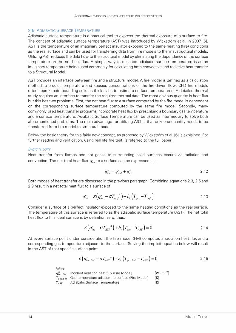
BASIC THEORY
Heat transfer from flames and hot gases to surrounding solid surfaces occurs via radiation and
convection. The net total heat flux tot
q„ to a surface can be expressed as:
tot rad cv
q q q= +„ „ „ 2.12
Both modes of heat transfer are discussed in the previous paragraph. Combining equations 2.3, 2.5 and
2.9 result in a net total heat flux to a surface of:
( ) ( )4
tot inc surf c gas surfq q T h T Tε σ= − + −„ „
2.13
Consider a surface of a perfect insulator exposed to the same heating conditions as the real surface.
The temperature of this surface is referred to as the adiabatic surface temperature (AST). The net total
heat flux to this ideal surface is by definition zero, thus:
( ) ( )4 0inc AST c gas ASTq T h T Tε σ− + − =„
2.14
At every surface point under consideration the fire model (FM) computes a radiation heat flux and a
corresponding gas temperature adjacent to the surface. Solving the implicit equation below will result
in the AST of that specific surface point.
( ) ( )4
, ,0
inc FM AST c gas FM ASTq T h T Tε σ− + − =„
2.15
With:
/-01,2344 Incident radiation heat flux (Fire Model) �W ∙ m�5�
�67�,23 Gas temperature adjacent to surface (Fire Model) �K�
�89: Adiabatic Surface Temperature �K�

FDS-2-ABAQUS: C++ MANAGED AUTOMATED PYTHON SCRIPTED CFD-FEM COUPLING
J.A. FEENSTRA 15
For the structural model (SM) the heat flux is computed based on the fire conditions predicted by the
fire model and the surface temperature as predicted by the structural model.
( ) ( )4
, , , , ,tot SM inc FM surf SM c gas FM surf SMq q T h T Tε σ= − + −„ „
2.16
With:
/ ; ,9344 Total heat flux (Structural Model) �W ∙ m�5�
/-01,2344 Incident radiation heat flux (Fire Model) �W ∙ m�5�
) Emissivity �−�
= Stefan Boltzmann Constant �W ∙ m�5 ∙ K�>�
ℎ1 Heat transfer coefficient �W ∙ m�5 ∙ K���
�67�,23 Gas temperature adjacent to surface (Fire Model) �K�
��@AB,93 Absolute Surface Temperature (Structural Model) �K�
Subtracting equation 2.16 from equation 2.15 results in a total net heat flux to the surface of:
( ) ( )4 4
, , ,tot SM AST surf SM c AST surf SMq T T h T Tεσ= − + −„
2.17

FDS-2-ABAQUS: C++ MANAGED AUTOMATED PYTHON SCRIPTED CFD-FEM COUPLING
J.A. FEENSTRA 17
3. APPROACH
The main goal of this thesis is to study the effectiveness (and feasibility) of the two way coupling of
CFD fire simulations to FE heat transfer and structural response analyses. In this chapter the general
approach to this topic will be clarified. Additionally it aims to explain the ‘what’ and the ‘how’ question,
as in what separate steps can be identified and how to address these steps.
Heat Transfer Analysis (A2)
Structural Response Analysis
(A3)
Fire Simulation (A1)
C1 C2
One-Way Coupling
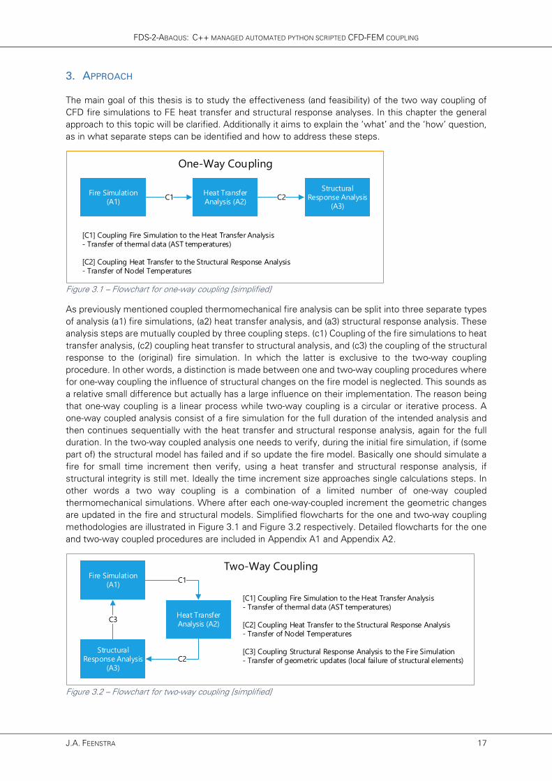
[C1] Coupling Fire Simulation to the Heat Transfer Analysis - Transfer of thermal data (AST temperatures)
[C2] Coupling Heat Transfer to the Structural Response Analysis- Transfer of Nodel Temperatures
Figure 3.1 – Flowchart for one-way coupling [simplified]
As previously mentioned coupled thermomechanical fire analysis can be split into three separate types
of analysis (a1) fire simulations, (a2) heat transfer analysis, and (a3) structural response analysis. These
analysis steps are mutually coupled by three coupling steps. (c1) Coupling of the fire simulations to heat
transfer analysis, (c2) coupling heat transfer to structural analysis, and (c3) the coupling of the structural
response to the (original) fire simulation. In which the latter is exclusive to the two-way coupling
procedure. In other words, a distinction is made between one and two-way coupling procedures where
for one-way coupling the influence of structural changes on the fire model is neglected. This sounds as
a relative small difference but actually has a large influence on their implementation. The reason being
that one-way coupling is a linear process while two-way coupling is a circular or iterative process. A
one-way coupled analysis consist of a fire simulation for the full duration of the intended analysis and
then continues sequentially with the heat transfer and structural response analysis, again for the full
duration. In the two-way coupled analysis one needs to verify, during the initial fire simulation, if (some
part of) the structural model has failed and if so update the fire model. Basically one should simulate a
fire for small time increment then verify, using a heat transfer and structural response analysis, if
structural integrity is still met. Ideally the time increment size approaches single calculations steps. In
other words a two way coupling is a combination of a limited number of one-way coupled
thermomechanical simulations. Where after each one-way-coupled increment the geometric changes
are updated in the fire and structural models. Simplified flowcharts for the one and two-way coupling
methodologies are illustrated in Figure 3.1 and Figure 3.2 respectively. Detailed flowcharts for the one
and two-way coupled procedures are included in Appendix A1 and Appendix A2.
Fire Simulation (A1)
Heat Transfer Analysis (A2)
Structural Response Analysis
(A3)
C1
C2
C3
Two-Way Coupling
[C1] Coupling Fire Simulation to the Heat Transfer Analysis - Transfer of thermal data (AST temperatures)
[C2] Coupling Heat Transfer to the Structural Response Analysis- Transfer of Nodel Temperatures
[C3] Coupling Structural Response Analysis to the Fire Simulation- Transfer of geometric updates (local failure of structural elements)
Figure 3.2 – Flowchart for two-way coupling [simplified]
ADDITIONALLY ASSESSING TWO-WAY COUPLING EFFECTIVENESS
18 MASTER THESIS
Based on the idea of a two-way coupling as a combination of multiple one-way coupling procedures.
The various steps in a one way coupling procedure are studied and later expended to two way coupling.
Basically it draws down to study the separate steps and then design coupling tools (scripts and
programs) to facilitate this one and two way coupling. But before these procedures can be modelled a
room should be designed as ‘case study’ for the coupling procedure. Therefore the first step comprises
the design of a model room and fire scenario. All steps are discussed separately in the remainder of
this chapter including references to chapters containing the information.
MODEL ROOM
A standard room model is developed to act as a starting point for the successive one- and two-way
coupling analyses. The design of the room is based on an office building comprising a thin-walled steel
structural façade. Both its geometric design and a corresponding fire scenario, based on its occupancy
class, are discussed in chapter 4.
FIRE SIMULATION (A1)
For the fire simulation the software Fire Dynamic Simulator (FDS) and its accompanying visualization
tool SmokeView are used. Using FDS the time and spatial varying thermal data is obtained for later use
in the heat transfer analysis. More specifically the obtained thermal data consist of the adiabatic surface
temperature of the structural elements under consideration. The concept of AST, as discussed in
section 2.5, is used to limit the data transfer from fire simulation to heat transfer model. A detailed
discussion on the fire simulation is included in chapter 5.
COUPLING FIRE SIMULATION TO THE HEAT TRANSFER ANALYSIS (C1)
The AST data from the fire simulation needs to be transferred to the subsequent heat transfer analysis.
The output from FDS cannot be input directly and should be pre-processed for use in the FE software.
It is important to note that the coupling from FDS to the HT simulation is assumed one-way, meaning
the resulting structural temperature is not fed back to the fire model. Since the structural system under
consideration is assumed adiabatic it will have constant temperature (room temperature) throughout
the duration of the simulation. Thereby influencing the temperature generation in the model. The overall
temperatures will be lower, compared to non-adiabatic behaviour, due to the constant temperature of
the studied structural system. The coupling of the fire simulation to the heat transfer is discussed in
section 6.3, the program developed to automate this coupling is discussed in section 7.3.
HEAT TRANSFER ANALYSIS (A2)
Finite Element software Abaqus is used to predict the thermal response of the structural system to the
thermal load from the fire. All three modes of heat transfer, as discussed in section 2.4 are taken into
account. The AST data is used to model convection and radiation to the structural model. Conduction
is accounted for as a material property. The assumed steel quality is S355 and all required material
properties comply with this selection. The heat transfer analysis is discussed in section 6.3.
COUPLING HEAT TRANSFER ANALYSIS TO THE STRUCTURAL RESPONSE ANALYSIS (C2)
The nodal temperature from the heat transfer analysis need to be transferred to the subsequent thermal
response analysis to model the response, and possible failure, of the structural system to the increase
in temperature. Both the heat transfer and structural response analysis are modelled using Finite
Element software Abaqus thereby simplifying this coupling. The output from the HT analysis can be
input directly in the SR analysis. Abaqus even allows the use of dissimilar meshes between the two
analyses. So no additional mapping tools are required. It is important to note that the coupling is
sequential, a one-way coupling. Both the heat generation due to rapid deformation and the disturbance
of the conductance flow field, due to occurrence of gaps, are neglected since both are assumed
negligible for the utilized time and structural scale. This coupling is discussed in more detail in section
6.4.

FDS-2-ABAQUS: C++ MANAGED AUTOMATED PYTHON SCRIPTED CFD-FEM COUPLING
J.A. FEENSTRA 19
STRUCTURAL RESPONSE ANALYSIS (A3)
Finite Element software Abaqus is used to predict the structural response to the temperature increase.
The nodal temperatures from the time varying nodal temperature data from the HT analysis is applied
as a boundary condition on the structural response model. Due to the temperature increase the steel
elements, assuming elastic plastic material behaviour, expand. This expansion is restricted thereby
generating thermal stresses to allow (some of) this expansion the structural elements could bend and
are therefore susceptible to buckling. This structural response could result in partial failure of the
structural system thereby influencing the fire propagation. It is important to note that for this initial study
the temperature dependency of the material properties are neglected. The structural response analysis
is discussed in section 6.4.
COUPLING STRUCTURAL RESPONSE ANALYSIS TO THE FIRE SIMULATION (C3)
This initial study focusses on the effect of (partial) failure of the structural system on the propagation of
the fire. It is not possible to model and study the effect of the relative small deformations (expansion
and buckling) since the precision of the fire model is limited to its discretization. A failure criteria is
required to determine if the structural system failed or not. For this study a simplified approach to failure
is assumed which checks if the von Mises Stress in the structural system exceeds the yield stress.
Geometric changes, based on aforementioned stress criterion, are then updated in the Fire, HT and SR
models. The failure criteria and the script to predict (plate) failure are discussed in section 7.7 .The
programs to automatically update the geometric changes in Fire Simulation, Heat Transfer, and
Structural Response analysis are discussed in sections 7.4 - 7.6 respectively.
PROGRAMS AND SCRIPTS
Given the multiple simulations and coupling steps the coupling procedure quickly becomes a tedious,
time consuming task. Not only because of the various iterations in the two-way coupled procedure but
also because of the ‘trial-and-error’ throughout the development. Therefore scripts and programs, using
programming language C++ and python, are developed to both facilitate the coupling steps and manage
the complete coupling procedure. A brief overview of the various programs and scripts is listed below.
For a detailed discussion on the scripts and programs is referred to chapter 7.
FDS-2-Abaqus Master program managing the two-way coupling.
reWriteAST2Py Program to rewrite FDS AST output for input in HT analysis.
upGeomFDS Program to update the FDS model.
upGeomHT Program to update the Heat Transfer model.
upGeomSR Program to update the Structural Response model.
PlateFailureCheck Script to check plate failure.

FDS-2-ABAQUS: C++ MANAGED AUTOMATED PYTHON SCRIPTED CFD-FEM COUPLING
J.A. FEENSTRA 21
4. EXPERIMENTAL SETUP: MODEL ROOM
A standard room model is developed to act as a starting point for the successive one- and two-way
coupling analyses. This room comprises thin-walled steel structural elements and acts as basis to proof
the principle of two way coupling. The design and function (occupancy class), thin-walled steel façade,
and fire scenario will be discussed consecutively in this chapter.
4.1 DESIGN
Thin walled steel façade systems are often
applied in office buildings and industrial
buildings. Therefore during the initial phase of
this project an office function was selected as
model room by association of thin walled steel
structural systems with industrial/office like
types of buildings
The traditional office building in the
Netherlands is highly standardized and
established according to fixed dimensions,
modules, and building grids. Industrial
manufactured prefabricated elements follow
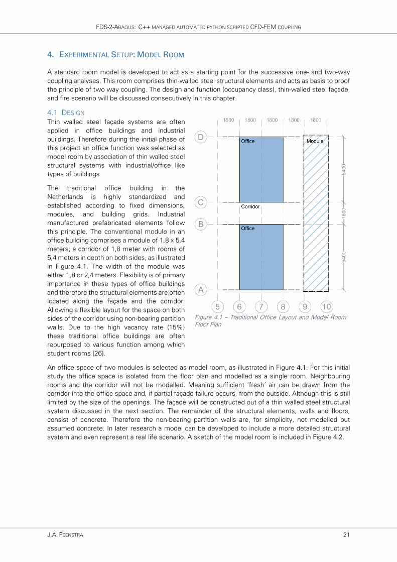
this principle. The conventional module in an
office building comprises a module of 1,8 x 5,4
meters; a corridor of 1,8 meter with rooms of
5,4 meters in depth on both sides, as illustrated
in Figure 4.1. The width of the module was
either 1,8 or 2,4 meters. Flexibility is of primary
importance in these types of office buildings
and therefore the structural elements are often
located along the façade and the corridor.
Allowing a flexible layout for the space on both
sides of the corridor using non-bearing partition
walls. Due to the high vacancy rate (15%)
these traditional office buildings are often
repurposed to various function among which
student rooms [26].
An office space of two modules is selected as model room, as illustrated in Figure 4.1. For this initial
study the office space is isolated from the floor plan and modelled as a single room. Neighbouring
rooms and the corridor will not be modelled. Meaning sufficient ‘fresh’ air can be drawn from the
corridor into the office space and, if partial façade failure occurs, from the outside. Although this is still
limited by the size of the openings. The façade will be constructed out of a thin walled steel structural
system discussed in the next section. The remainder of the structural elements, walls and floors,
consist of concrete. Therefore the non-bearing partition walls are, for simplicity, not modelled but
assumed concrete. In later research a model can be developed to include a more detailed structural
system and even represent a real life scenario. A sketch of the model room is included in Figure 4.2.
Figure 4.1 – Traditional Office Layout and Model Room Floor Plan
ADDITIONALLY ASSESSING TWO-WAY COUPLING EFFECTIVENESS
22 MASTER THESIS
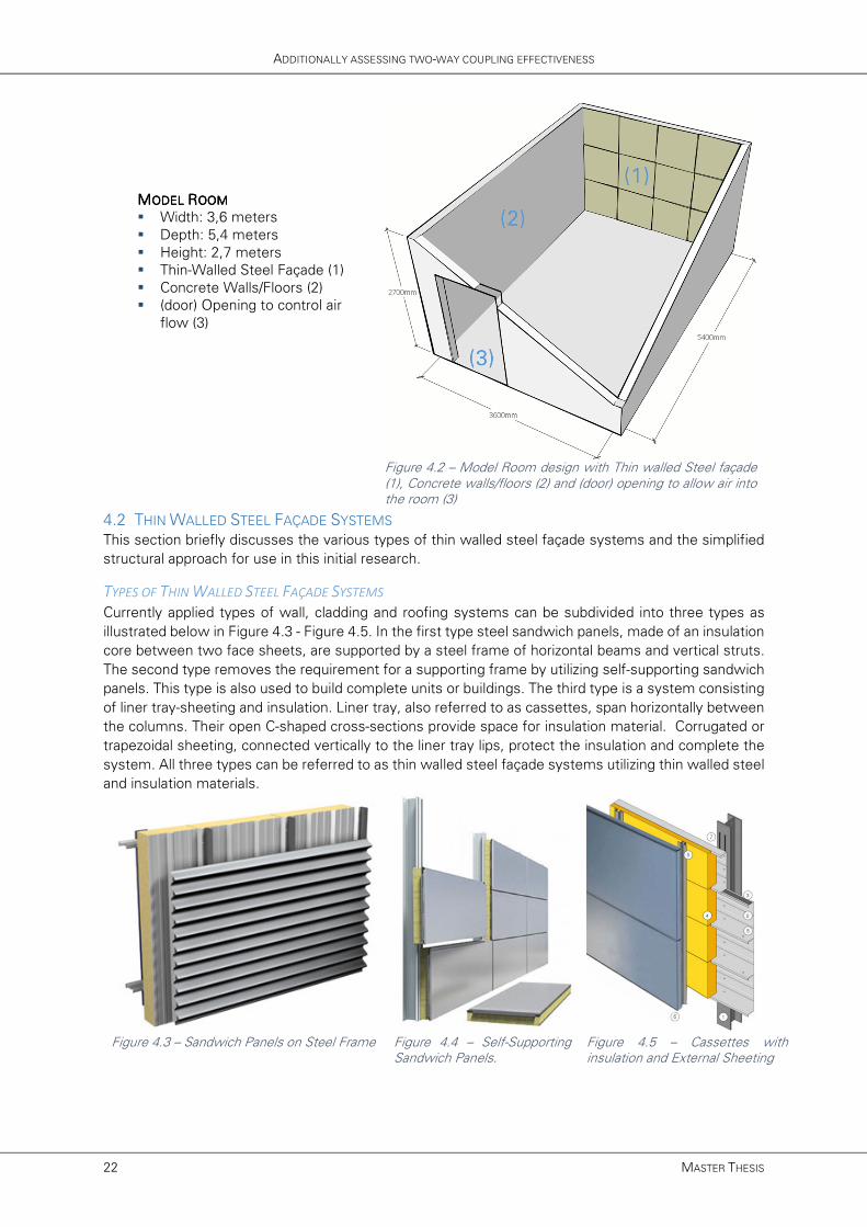
MMMMODEL ODEL ODEL ODEL RRRROOMOOMOOMOOM
� Width: 3,6 meters
� Depth: 5,4 meters
� Height: 2,7 meters
� Thin-Walled Steel Façade (1)
� Concrete Walls/Floors (2)
� (door) Opening to control air
flow (3)
Figure 4.2 – Model Room design with Thin walled Steel façade (1), Concrete walls/floors (2) and (door) opening to allow air into the room (3)
4.2 THIN WALLED STEEL FAÇADE SYSTEMS
This section briefly discusses the various types of thin walled steel façade systems and the simplified
structural approach for use in this initial research.
TYPES OF THIN WALLED STEEL FAÇADE SYSTEMS
Currently applied types of wall, cladding and roofing systems can be subdivided into three types as
illustrated below in Figure 4.3 - Figure 4.5. In the first type steel sandwich panels, made of an insulation
core between two face sheets, are supported by a steel frame of horizontal beams and vertical struts.
The second type removes the requirement for a supporting frame by utilizing self-supporting sandwich
panels. This type is also used to build complete units or buildings. The third type is a system consisting
of liner tray-sheeting and insulation. Liner tray, also referred to as cassettes, span horizontally between
the columns. Their open C-shaped cross-sections provide space for insulation material. Corrugated or
trapezoidal sheeting, connected vertically to the liner tray lips, protect the insulation and complete the
system. All three types can be referred to as thin walled steel façade systems utilizing thin walled steel
and insulation materials.
Figure 4.3 – Sandwich Panels on Steel Frame
Figure 4.4 – Self-Supporting Sandwich Panels.
Figure 4.5 – Cassettes with insulation and External Sheeting

FDS-2-ABAQUS: C++ MANAGED AUTOMATED PYTHON SCRIPTED CFD-FEM COUPLING
J.A. FEENSTRA 23
SIMPLIFYING THE THIN WALLED FAÇADE
The detailed modelling of thin walled steel façade systems is outside the scope of this initial research.
But rather focusses on the effectiveness of two way coupling compared to one-way coupling and other
types of fire simulations. A thin walled steel façade system of sandwich panels on a steel frame is
selected as structural system. The panels are simplified to a single steel plate. Failure of a panel results
in a direct connection to the outside (and thereby influencing the fire). The second simplification step is
modelling the steel frame as boundary conditions, thereby omitting its modelled geometry from the
calculations. The simplification procedure is illustrated in Figure 4.6 below, the full wall can be modelled
as twelve separate panels.
Figure 4.6 - Simplification of sandwich panels on thin walled steel frame
4.3 FIRE SCENARIO
In this section a fire scenario is designed based on literature and regulations as previously discussed in
section 2.2. Based on Table 2.1 a fire load density of /B- = 700 MJ m5⁄ is selected for the office function
(average of ~90% fractile). Based on the floor plan of the model room the net heat of combustion DB-
can be expressed as
4
700 3,6 5, 4
1,36 10 MJ
fi fi fiQ q A= ⋅
= ⋅ ⋅
= ⋅
The limit value for the heat release rate for an office function is 250 kW m5⁄ . A fully developed fire is
assumed with a linear decreasing decay phase initialized when 70% of the combustibles have been
consumed [19]. The corresponding durations for these fully developed and decay phase can be
expressed with equation 2.18. The fire scenario is summarized below in Figure 4.7.
1
122
0,7
0,3
fi f fi
fi f fi
t A HRR Q
t A HRR Q
⋅ ⋅ = ⋅
⋅ ⋅ ⋅ = ⋅ 2.18

ADDITIONALLY ASSESSING TWO-WAY COUPLING EFFECTIVENESS
24 MASTER THESIS
FFFFIRE IRE IRE IRE SSSSCENARIOCENARIOCENARIOCENARIO
� /B- = 700 MJ m5⁄
� DB- = 13600MJ
� FB- = 3650s
� FG = 10s Duration flashover phase
� F� = 1960s Duration fully-developed phase
� F5 = 1680s Duration decay phase
Figure 4.7 – Fire Scenario for Model Room
0
50
100
150
200
250
300
0 900 1800 2700 3600 4500H
ea
t R
ele
ase
Ra
te [
kW
/m2]
Time t [s]
FDS-2-ABAQUS: C++ MANAGED AUTOMATED PYTHON SCRIPTED CFD-FEM COUPLING
J.A. FEENSTRA 25
5. SIMULATING FIRE WITH FIRE DYNAMIC SIMULATOR
This chapter discusses the fire simulation using Fire Dynamic Simulator (FDS). The first section describe
briefly the fire dynamic simulator software and its accompanying visualization tool SmokeView. In the
subsequent sections both the coding and running of an FDS simulation are discussed in detail. The last
section discusses the modification of the fire model during the simulation.
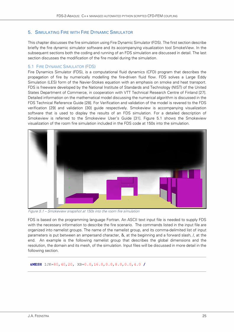
5.1 FIRE DYNAMIC SIMULATOR (FDS)
Fire Dynamics Simulator (FDS), is a computational fluid dynamics (CFD) program that describes the
propagation of fire by numerically modelling the fire-driven fluid flow. FDS solves a Large Eddy
Simulation (LES) form of the Navier-Stokes equation with an emphasis on smoke and heat transport.
FDS is freeware developed by the National Institute of Standards and Technology (NIST) of the United
States Department of Commerce, in cooperation with VTT Technical Research Centre of Finland [27].
Detailed information on the mathematical model discussing the numerical algorithm is discussed in the
FDS Technical Reference Guide [28]. For Verification and validation of the model is revered to the FDS
verification [29] and validation [30] guide respectively. Smokeview is accompanying visualization
software that is used to display the results of an FDS simulation. For a detailed description of
Smokeview is referred to the Smokeview User’s Guide [31]. Figure 5.1 shows the Smokeview
visualization of the room fire simulation included in the FDS code at 150s into the simulation.
Figure 5.1 – Smokeview snapshot at 150s into the room fire simulation
FDS is based on the programming language Fortran. An ASCII text input file is needed to supply FDS
with the necessary information to describe the fire scenario. The commands listed in the input file are
organized into namelist groups. The name of the namelist group, and its comma-delimited list of input
parameters is put between an ampersand character, &, at the beginning and a forward slash, /, at the
end. An example is the following namelist group that describes the global dimensions and the
resolution, the domain and its mesh, of the simulation. Input files will be discussed in more detail in the
following section.
&MESH IJK=80,40,20, XB=0.0,16.0,0.0,8.0,0.0,4.0 /

ADDITIONALLY ASSESSING TWO-WAY COUPLING EFFECTIVENESS
26 MASTER THESIS
The aim of FDS is to solve practical fire problems in fire engineering and to provide a tool for studying
fire dynamics and propagation. Its first version was released to the public in February 2000. Its main
applications comprise the design of smoke handling systems and sprinkler/detector activation studies
and the reconstruction of industrial and residential fires.
FDS version 6.1.12 is used throughout this report.
5.2 WRITING AN FDS INPUT FILE
This paragraph discussed the writing (and running) of an FDS input file. Complete FDS input file with
detailed explanation are included in Appendix X. For additional information on writing and running FDS
input files and all possible namelist groups and attributes, is referred to the FDS User’s Guide [27] .
FILE STRUCTURE
An FDS Input File (*.fds) is written from &HEAD to &TAIL. In between its &HEAD and &TAIL the namelist
records can be included in any order in the input file. Typically the namelist records are organized in a
systematic way with general information near the top while detailed information, like obstructions and
devices are listed towards the end. Each time FDS processes a namelist group it scans the whole input
file. It is advised to liberally include comments to increase the (re)readability of the input files. Ensure
that these comments do not fall within the namelist records by preceding them with one (or more)
forward slash characters.
The namelist group &HEAD contains two attributes: CHID and TITLE. CHID is a string of up to 30
characters used to tag output files. The TITLE attribute is a string of up to 60 characters describing the
simulation. These attributes are of great importance in organizing various simulations. The &TAIL
namelist record ensures that FDS reads the entire file. The &HEAD is often followed by the &TIME
namelist group describing the initiation (T_BEGIN) and duration (T_END) of the simulation. If T_BEGIN
and T_END are equal to each other FDS only generates the model set-up allowing one to check the
model set-up before running the simulation.
For illustrative purposes a (very) generalized input file is listed below.
&HEAD CHID='FirstFDS', TITLE='My First FDS Simulation' / &TIME T_END=300 / // General Information
// Detailed Information
&TAIL /
GEOMETRY
The FDS calculations are performed within a domain that is made of rectilinear volumes called meshes.
Each mesh is divided into rectangular cells. Increasing the number of cells increases the resolution and
required computational time of the simulation. This computational domain is defined using the &MESH
namelist group.
A mesh is a rectangular box with a coordinate system that conforms to the right hand rule. Its
dimensions are defined by the attribute XB, containing a string of six numbers describing the origin and
opposite corner of the domain. The first, third and fifth value define the origin point and the second,
fourth, and sixth the opposite corner. The attribute IJK describes the number of cells within the mesh
in respectively the x, y, and z direction. For instance the input line listed below creates a domain of 39.0 3.6 2.7 mxyz = ⋅ ⋅ subdivided into cells of
30.3 0.3 0.3 mxyz = ⋅ ⋅
&MESH IJK=30,12,9, XB=0.0,9.0,0.0,3.6,0.0,2.7 /

FDS-2-ABAQUS: C++ MANAGED AUTOMATED PYTHON SCRIPTED CFD-FEM COUPLING
J.A. FEENSTRA 27
The envelope of the domain consist of external walls. Additional obstructions describing the geometry
of the model can be introduced with the &OBST namelist group. Each &OBST line describes a rectangular
solid in the flow domain. Like the domain it is defined using the attribute XB containing a string of six
numbers defining the origin and opposite corner of the rectangular obstruction. The (surface) boundary
conditions of the obstruction can be specified with the attribute SURF_ID, which refers to a
corresponding &SURF line. The &SURF namelist group is discussed in more detail below. The level of
detail of the model and its obstructions is limited by cell size. In other words: the dimensions of
obstructions are scaled and fitted to nearby cells.
It is self-evident that when one wants to model a wall containing a door or window it would be a tedious
task to split this wall in separate rectangular components. The &HOLE namelist group can be used to
carve a hole out of an existing obstruction or set of obstructions. As with &OBST the attribute XB is
used to define the size and location of the &HOLE object. Any solid mesh cells intersecting with the
object are removed.
The &SURF namelist group is used to define attributes for all solid surfaces or openings within the flow
domain. The default boundary condition is that of an inert wall at fixed temperature. Each &SURF line is
identified with an identification string ID=’<name>’. This string is used to reference to the &SURF line
by the &OBST and &VENT namelist groups using the character string SURF_ID=’…’. If a SURF_ID is
omitted from an &OBST or &VENT line the default surface properties are applied. One can overwrite the
boundary condition by including DEFAULT=.TRUE. on the &SURF line.
Material properties can be prescribed using the &MATL namelist group. Various material properties like
density, conductivity, specific heat, and emissivity can be prescribed. The &MATL line is identified with
an identification string ID=’<name>’. This string is used to reference to the &MATL line by the &SURF
line (which in turn is referred to by a &VENT or &OBST line).
The &VENT namelist group is used to apply a particular boundary condition to a rectangular patch on a
solid surface. Historically the &VENT attribute allowed for air to be blown into or sucked out of the
computational domain but has since evolved well beyond its initial role. The attribute XB is used to
describe the dimension and location of the patch. Since a plane is described two of the six coordinates
must be the same within the XB attribute. Alternatively, the attribute MB (Mesh Boundary) can be used
to easily select limiting planes of the mesh. As previously discussed each &VENT includes a character
string SURF_ID referring to a set of boundary conditions described on the corresponding &SURF line.
A special type of (reserved) SURF_ID is ‘OPEN’ denoting a passive opening to the outside and can
only be used if the &VENT is applied to an exterior boundary of the computational domain.
Combining the namelist groups discussed in this section, the input lines below create a concrete box
with a large opening in direct contact with the outside. The Smokeview visualization is shown in
Figure 5.2.

ADDITIONALLY ASSESSING TWO-WAY COUPLING EFFECTIVENESS
28 MASTER THESIS
…
&MESH IJK=30,12,9, XB=0.0,9.0,0.0,3.6,0.0,2.7 / &SURF ID='CONCRETE_S', MATL_ID='CONCRETE_M', THICKNESS=0.3, COLOR='GRAY', DEFAULT=.TRUE. / &MATL ID='CONCRETE_M', DENSITY=1800, CONDUCTIVITY=1.15, SPECIFIC_HEAT=1.00, EMISSIVITY=0.80, / &OBST XB=1.8,1.8,0.0,3.6,0,2.7 / &HOLE XB=1.6,2.0,0.6,3.0,0.0,2.1 / &VENT XB=0.0,1.8,0.0,3.6,0.0,0.0, SURF_ID='OPEN' / &VENT XB=0.0,1.8,0.0,3.6,2.7,2.7, SURF_ID='OPEN' / &VENT XB=0.0,1.8,0.0,0.0,0.0,2.7, SURF_ID='OPEN' / &VENT XB=0.0,1.8,3.6,3.6,0.0,2.7, SURF_ID='OPEN' / &VENT MB='XMIN', SURF_ID='OPEN' /
…
Figure 5.2 – Basic FDS Model Utilizing Geometry Namelist Groups
SIMULATING FIRE
In section 4.3 a fire scenario was developed. This fire scenario needs to be modelled in FDS. For
example
…
&SURF ID='fire',HRRPUA=250 ,TMP_FRONT=20,COLOR='RED' / &VENT XB=1.8,7.2,0.0,3.6,0.0,0.0, SURF_ID='fire' /
…
generates a fully developed fire on the entire surface area of the office floor. To accurately model the
fire scenario discussed previously the &RAMP namelist group is used. The input lines

FDS-2-ABAQUS: C++ MANAGED AUTOMATED PYTHON SCRIPTED CFD-FEM COUPLING
J.A. FEENSTRA 29
…
&SURF ID='fire',HRRPUA=250,RAMP_Q='fire_r',TMP_FRONT=20,COLOR='RED' / &RAMP ID='fire_r',T= 0,F=0. / &RAMP ID='fire_r',T= 10,F=1. / &RAMP ID='fire_r',T=1970,F=1. / &RAMP ID='fire_r',T=3650,F=0. / &VENT XB=1.8,7.2,0.0,3.6,0.0,0.0, SURF_ID='fire' /
…
accurately describe the fire scenario. The heat release increases linearly from 0 to 250 kW/m2 in the first
10 seconds of the simulation and remains constant for 1960 seconds. After that it drops linearly to 0
kW/m2 over the course of 1680 seconds. If the simulation duration would be increased the heat release
would remain constant at 0 kW/m2, the last defined value.
The heat released by the aforementioned input lines cannot be generated out of thin air but need to be
generated by a combustion reaction. This combustion reaction has been discussed in detail in 4.3 but
needs to be included in the input file. Combustion reactions are prescribed in FDS using the &REAC
namelist group.
The default combustion model in FDS is that of single-step mixing controlled combustion, in which the
reaction of fuel and oxygen is infinitely fast and only controlled by mixing, hence the label. This approach
is referred to as the ‘simple chemistry’ combustion model. FDS considers a single fuel species that is
composed primary of Carbon (C), Hydrogen (H), Oxygen (O), and Nitrogen (N) reacting with oxygen (O2)
to form Water (H2O), Soot (mainly C), Carbon dioxide (CO2), Carbon monoxide (CO), and Nitrogen (N2).
This ‘simple chemistry’ approach can be expressed in a chemical equation as shown in equation 2.19
2 2 2 2x y z v 2 2 2 2C H O N O CO H O CO Soot N
O CO H O CO S Nv v v v v v+ → + + + + 2.19
The stoichiometric coefficients are automatically calculated by FDS. To accurately calculate these values
from the chemical formula the post combustion yields of CO, soot and volume fraction of Hydrogen in
the soot, need to be defined. The default values for the post combustion yields are 0. The total energy
released by the combustion can be computed by taking the sum of the net change in mass for each
species multiplied by the species enthalpy of formation. Various enthalpy of formations values are
included in FDS and listed in table 11.1 in the FDS User’s Guide [27]. If the fuel species is not included
in table 11.1 of the FDS User’s Guide there are various options to specify the missing enthalpies. In the
first option one can specify the unknown enthalpy on a separate species, &SPEC, line in kJ/mol.
Secondly, if only the enthalpy of formation of the fuel is missing, the heat of combustion can be directly
specified on the &REAC line in kJ/kg. Lastly, if enthalpies are missing and no heat of combustion is
specified, the heat of combustion is computed based on the amount of energy released per unit mass
of oxygen consumed.
The combustion reaction discussed in section 4.3 can be included by defining both a &REAC line and
defining the enthalpy of formation of cellulose on a &SPEC line as listed below. Alternatively the heat
of combustion could be directly specified on the &REAC line.
…
&SPEC ID = 'CELLULOSE',
FORMULA = 'C4H6O3', MW = 102.0886 ENTHALPY_OF_FORMATION=-5.13E2 / &REAC FUEL = 'CELLULOSE' /
…

ADDITIONALLY ASSESSING TWO-WAY COUPLING EFFECTIVENESS
30 MASTER THESIS
Combining the namelist groups discussed in this section a (ramp based) fire can be simulated as
illustrated with the Smokeview visualization in Figure 5.3.
Figure 5.3 – Basic FDS Fire Simulation with Cellulose Combustion Reaction
Alternatively one can model an interior using &OBST and assigning calorific values in the &MATL namelist
group. This allows one to accurately model a fire compartment, its interior and its encompassed calorific
energy. This will not be discussed further but a good example is found in the room_fire model included
in the FDS installation.
SPECIFYING OUTPUT
To effectively couple the fire simulation to a subsequent heat transfer analysis AST data needs to be
extracted at specific locations in the fire model. By default FDS outputs the total Heat Release and
related quantities to an output file called CHID_hrr.csv. Additional data can be requested using
devices designated via the &DEVC namelist group. Devices can be used to record some location
dependent quantity of the simulated environment or to trigger events. This section will focus on
obtaining specific data using devices. As an example the line
…
&DEVC XYZ=7.2,2.475,1.125, QUANTITY='ADIABATIC_SURFACE_TEMPERATURE',
ID='AST_1A', IOR=-1 /
…
creates a device at position XYZ that records the QUANTITY adiabatic surface temperature. A device is
characterized with an unique character string ID. This descriptive string is used to identify the device
in the output files. IOR is an abbreviation of Index of Orientation and should be defined for any device
placed on the surface of a solid. Its value depicts the direction the device points, where the values ±1,
±2, or ±3 correspond to respectively the positive or negative x,y, or z direction. The above device is
actually positioned on the back wall of the fire model illustrated in Figure 5.3 hence the ‘-1’ direction.
Various AST output devices should be included in the input file to obtain sufficient temperature data for
use in the subsequent thermomechanical analysis.
An overview of frequently used QUANTITY attributes is given in table 16.3 of the FDS User’s Manual.
For additional reading and information on defining more complex devices like smoke detectors and
sprinklers is referred to chapter 15 of the FDS User’s Manual [27].

FDS-2-ABAQUS: C++ MANAGED AUTOMATED PYTHON SCRIPTED CFD-FEM COUPLING
J.A. FEENSTRA 31
RUNNING THE SIMULATION
FDS is run from command prompt by first locating the correct path and then using the command:
fds inputfile.fds
The string contained in the CHID attribute in the &HEAD namelist group of the input file is associated
with the ouput files generated by the simulation. Detailed diagnostic information is automatically written
to a file CHID.out. Screen output can be redirected to a file by the command
fds inputfile.fds > inputfile.err
Alternatively one can create a batch file (*.bat) in the folder of the input file and include the code above
the directly run the simulation without the necessity to browse to the path using the command prompt.
An example of such a batch script is listed below. The pause command interrupts closing of the cmd
prompt until ‘any key’ is pressed. This way one can check the simulation (or possible errors) before
closing it.
It is also possible to associate the *.fds file extension with FDS, if associated one can run the simulation
by double clicking the *.fds file (Windows 10 automatically associates *.fds files with FDS). Keep in
mind that rerunning a simulation without changing the CHID attribute in the &HEAD namelist group will
overwrite previous output.
5.3 MODIFYING THE FIRE MODEL DURING SIMULATION
In order to successfully perform the two way coupling of a fire model and a thermomechanical analysis
one needs to iterate through the various analysis steps. So first simulate for x iterations and checking
for plate failure in subsequent thermomechanical analysis. If failure occurs update the FDS model and
continue with the next iteration. The ideal case being when x = 1. Independent of the iteration size one
should be able to stop the calculation wait for the output of the thermomechanical analysis and possibly
remove a panel based on this outcome and continue to the next iteration. These steps: stopping the
simulation, restarting the simulation and changing the model during (or in between) simulations are
required in order to be able to perform a two-way coupled thermomechanical analysis and will be
discussed in the remainder of this paragraph.
INTERRUPTING A FDS SIMULATION
There are two ways to interrupt (or kill) a FDS simulation. The first possibility is by creating a dummy
file CHID.stop in the simulation path. In which CHID refers to the tag string defined in the &HEAD
namelist group that is used to name all output files. The second possibility is by using a device (&DEVC)
to trigger a control function (&CTRL). As an example the following lines will interrupt the simulation
when the simulation time reaches 300 seconds.
…
&DEVC XYZ=0.1,0.1,0.1, ID='Trigger', SETPOINT=300.0, QUANTITY='TIME' / &CTRL ID='Stop_Simulation', FUNCTION_TYPE='KILL', INPUT_ID='Trigger' /
…

ADDITIONALLY ASSESSING TWO-WAY COUPLING EFFECTIVENESS
32 MASTER THESIS
RESTARTING A FDS SIMULATION
FDS requires a restart file CHID.restart in order to restart a simulation after interruption. FDS can
create restart files periodically by including the attribute DT_RESTART=’Seconds’ on the &DUMP line
in the input file. This is especially valuable in very long simulations as a safety measure against random
crashes or a power outage. As an example the following line should be included to create restart files
every 300 seconds (simulation time, not real time).
…
&DUMP DT_RESTART=300.0 /
…
Alternatively a restart file can be generated with a &CNTR function and a corresponding &DEVC trigger,
similar to the KILL function discussed previously. As an example the following lines will interrupt the
simulation when the simulation time reaches 300 seconds, and at the same time, create a restart file.
…
&DEVC XYZ=0.1,0.1,0.1, ID='Trigger', SETPOINT=300.0, QUANTITY='TIME',
LATCH=.FALSE. / &CTRL ID='Stop_Simulation', FUNCTION_TYPE='KILL', INPUT_ID='Trigger', LATCH=.FALSE. / &CTRL ID='Create_Restart', FUNCTION_TYPE='RESTART', INPUT_ID='Trigger', LATCH=.FALSE. /
…
Since multiple changes of state are required the attribute LATCH=.FALSE. is included. A latch can only
change state a single time and therefore, if excluded, the simulation would not be interrupted and no
restart file would be generated after the first iteration.
To restart a simulation from a restart file the line the attribute RESTART=.TRUE. should be included on
the &MISC line. The output from the restarted simulation is appended to the output files from the
original simulation. Alternatively the attribute RESTART_CHID=’some_name' can be specified on the
&MISC line to restart the simulation from a specific restart file and write the output to output files tagged
with the CHID as defined in the &HEAD line.
The FDS user manual specifically states that between stops and restarts major changes cannot be
made to the fire model. The changes are limited to those attributes that do not directly influence the
existing flow field. The removal (or addition) of obstructions would directly influence the flow field and
are therefore not allowed. Meaning it is impossible to simply delete the obstructions that, as a result
of the subsequent thermos-mechanical analysis, have failed. A solution is discussed in the next section.
TIME-CONTROLLED OBJECT REMOVAL
Similar to the device trigger controlling the previously discussed KILL and RESTART function a device
can be defined to (de)activate an obstruction. The following lines will deactivate the obstruction
Plate_08 after 300 seconds.
…
&OBST XB=7.2,7.2,0.9,1.8,0.9,1.8, DEVC_ID='Plate_08' /
&DEVC XYZ=0.1,0.1,0.1, ID='Plate_08', SETPOINT=300.0, QUANTITY='TIME',
INITIAL_STATE=.TRUE. / …
FDS-2-ABAQUS: C++ MANAGED AUTOMATED PYTHON SCRIPTED CFD-FEM COUPLING
J.A. FEENSTRA 33
Time-Controlled Object Removal can be utilized as a solution to the inability to remove obstruction
between the stop and restart of a simulation. Initially a unique timed removal should be defined for all
plates with a trigger time outside the simulation time. Given a simulation with a total simulation time of
T_END=3650, the following lines define the deactivation of Plate_08 after 3700 seconds. Since the
simulation only last for 3650 seconds the plate will never be removed and will still be there at the end
of the simulation.
… &TIME T_END=3650 / &OBST XB=7.2,7.2,0.9,1.8,0.9,1.8, DEVC_ID='Plate_08' / &DEVC XYZ=0.1,0.1,0.1, ID='Plate_08', SETPOINT=3700.0, QUANTITY='TIME',
INITIAL_STATE=.TRUE. /
…
Assuming above lines are used in a two-way coupled thermo-mechanical simulation. After a couple of
iteration steps at, for instance, 1200 seconds the mechanical analysis returns failure of Plate_08.
Before restarting the FDS simulation the SETPOINT attribute should be changed to remove the plate
from the simulation. The removal can occur directly at the restart of the simulation since FDS ‘knows’,
due to the time controlled object removal device, that the obstruction will be removed at some point.
Thereby invalidating the non-altering for the existing flow field. The following lines show the updated
lines for the next iteration of the input file incorporating the removal of the plate after the mechanical
analysis returned failure of Plate_08.
… &TIME T_END=3650 / &OBST XB=7.2,7.2,0.9,1.8,0.9,1.8, DEVC_ID='Plate_08' / &DEVC XYZ=0.1,0.1,0.1, ID='Plate_08', SETPOINT=1200.0, QUANTITY='TIME',
INITIAL_STATE=.TRUE. /
…
With the namelist groups and corresponding attributes discussed in this chapter it is possible to create,
run, interrupt and restart FDS simulations. In addition obstructions can be removed at a moment in time
slightly after obstruction failure is measured by the subsequent mechanical analysis. This removal is
governed by time-controlled object removal. It is self-evident that the increase in iterations (coupling
cycles) limits the time difference between the measured failure time and the moment in time at which
the panel is removed from the simulation. For a few iterations this is possible to do by hand but soon
this becomes a tedious task. Therefore this process should be automated. For additional reading on the
coupling programs used in the two-way coupling of fire simulations to the thermomechanical analysis
is referred to chapter 7.


FDS-2-ABAQUS: C++ MANAGED AUTOMATED PYTHON SCRIPTED CFD-FEM COUPLING
J.A. FEENSTRA 35
6. ABAQUS ANALYSIS
The finite element code used throughout this study is Abaqus. This software will be discussed briefly
in the following section. In the remainder of the chapter the basic model setup, the heat transfer model
and analysis, the structural response model and analysis, multiple plate models, restart analysis, and
plate removal will be discussed sequentially.
6.1 ABAQUS CAE
The Abaqus Complete Abaqus Environment (CAE) is part of the Abaqus product suite for finite element
analysis and computer aided design. The full suite offers powerful and complete solutions for both
routine and sophisticated engineering problems covering a vast spectrum of industrial applications. The
first version of Abaqus was released in 1978 by a company called HKS, renamed to Abaqus inc. in 2002
and acquired by Dassault Systèmes in 2005 [32].
The finite element method is a numerical method for solving systems of differential equations to predict
structural response. The finite-element method divides a structural model in a limited, hence the name
finite, number of elements. These elements are interconnected through nodes and governed by
boundary conditions. The connected nodes, for instance, should displace equally. By dividing the
structural model in a finite number of elements the complex differential equations can be approximated
by matrix calculations. By increasing the number of elements the solution converges to the analytical
solution.
The approach to a finite element problem can be split in three consecutive steps as illustrated in Figure
6.1. The first step is pre-processing, a representative model is defined and subjected to boundary
conditions describing the problem at hand. In the simulation a Finite element solver is used to obtain
numerical solutions to the given problem. During post-processing the previously obtained results are
used to interpret the response of the model to the boundary conditions. Abaqus CAE is used for the
pre-processing and post-processing of the finite element analysis. For the simulation either the
Abaqus/Standard or Abaqus/Explicit finite element solver is used. In which the former employs an
implicit and the latter an explicit integration scheme.
Pre-Processing
(Modelling)
Abaqus/CAE
Simulation
Abaqus/Standard or
Abaqus/Explicit
Post-processing
(Visualization)
Abaqus/CAE
Figure 6.1 – Approach to a finite element problem.
Each step in the above approach is challenging on its own. One could state that a basic understanding
of the modelling, simulation and visualization process is required to obtain valid results. The extensive
documentation included in Abaqus CAE, and available online, could be of help in this process. This
documentation consist of guides on modelling and visualization, analysis, examples, benchmarks and
basic tutorials. In addition reference guides on theory, verification and scripting are available [33].
Abaqus is based on program language Fortran. In the pre-processing phase one either inputs all
parameters directly in the GUI, or by using scripts based on the Python language. Some tasks would
be practically impossible or very time consuming when only using the GUI. Abaqus uses programing
language C for writing the output database. A basic understanding of these different programming
languages helps in efficiently using Abaqus to solve problems.
Abaqus CAE version 6.14 is used throughout this report.
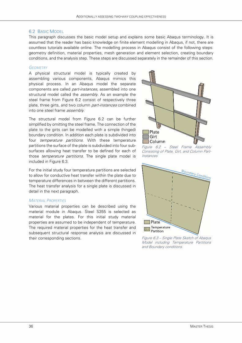
ADDITIONALLY ASSESSING TWO-WAY COUPLING EFFECTIVENESS
36 MASTER THESIS
6.2 BASIC MODEL
This paragraph discusses the basic model setup and explains some basic Abaqus terminology. It is
assumed that the reader has basic knowledge on finite element modelling in Abaqus, if not, there are
countless tutorials available online. The modelling process in Abaqus consist of the following steps:
geometry definition, material properties, mesh generation and element selection, creating boundary
conditions, and the analysis step. These steps are discussed separately in the remainder of this section.
GEOMETRY
A physical structural model is typically created by
assembling various components, Abaqus mimics this
physical process. In an Abaqus model the separate
components are called part-instances, assembled into one
structural model called the assembly. As an example the
steel frame from Figure 6.2 consist of respectively three
plate, three girts, and two column part-instances combined
into one steel frame assembly.
The structural model from Figure 6.2 can be further
simplified by omitting the steel frame. The connection of the
plate to the girts can be modelled with a simple (hinged)
boundary condition. In addition each plate is subdivided into
four temperature partitions. With these temperature
partitions the surface of the plate is subdivided into four sub-
surfaces allowing heat transfer to be defined for each of
those temperature partitions. The single plate model is
included in Figure 6.3.
For the initial study four temperature partitions are selected
to allow for conductive heat transfer within the plate due to
temperature differences in between the different partitions.
The heat transfer analysis for a single plate is discussed in
detail in the next paragraph.
MATERIAL PROPERTIES
Various material properties can be described using the
material module in Abaqus. Steel S355 is selected as
material for the plates. For this initial study material
properties are assumed to be independent of temperature.
The required material properties for the heat transfer and
subsequent structural response analysis are discussed in
their corresponding sections.
Figure 6.2 – Steel Frame Assembly Consisting of Plate, Girt, and Column Part-Instances
Figure 6.3 – Single Plate Sketch of Abaqus Model including Temperature Partitions and Boundary conditions.

FDS-2-ABAQUS: C++ MANAGED AUTOMATED PYTHON SCRIPTED CFD-FEM COUPLING
J.A. FEENSTRA 37
MESH GENERATION
As previously discussed in finite element analysis the model is divided in a finite number of elements
for which the complex differential equations can be approximated by matrix calculations. The
subdivision into separate elements is called the mesh. Each element in the mesh is then assigned an
element type with corresponding element properties. There are a wide range of element types available
in Abaqus for which is referred to the Abaqus Analysis User’s Guide chapters 27 – 33 [33].
Shell elements are often used when the thickness of the shell is small
compared to the typical dimensions in the shell surface. With shell elements
a three dimensional continuum is approximated using a, more economical,
two-dimensional theory. Shell elements will be used throughout this study
since the nature of the model ‘plates on a frame’, have a relative small
thickness compared to its surface dimensions.
The element type DS8 will be used for the heat transfer analysis and the
element type S8R for the sequentially coupled stress/displacement analysis.
These elements are illustrated in Figure 6.4 and Figure 6.5. In Abaqus the
element name identifies its primary element characteristics. Element DS8 is
an 8-node quadrilateral Heat Transfer Shell Element and element S8R is an
8-node doubly curved Stress/displacement shell element with reduced
integration. Reduced-order integration allow for fast and cheap calculation of
the element matrices but may have significant effect on the accuracy of the
element.
Stresses (and temperatures) are accurately calculated in the integration
(Gauss) points using Gaussian quadrature method to numerically
approximate the integrals. The locations of the shell elements are illustrated
in Figure 6.4 and Figure 6.5. Section Points are the equally spaced integration
points over the thickness of the shell. The typical number of section points
is five.
BOUNDARY CONDITIONS
The step module controls the incrementation and duration of the simulation. Boundary conditions (and
loads) are applied during the initial step or a newly defined step. The heat transfer analysis is
independent of support boundary conditions since no displacement is involved. For the structural
response analysis hinged (line) supports are imposed on the top and bottom edge of the plate to
simulate the connection of the plate to the girts (see also Figure 6.4 and Figure 6.5). The load in the
heat transfer analysis is controlled by the convective and radiative flux as result of the adiabatic surface
temperature from the corresponding FDS fire simulation. The load step in the structural response
analysis are governed by the nodal temperatures from the heat transfer analysis inducing thermal
expansion resulting in thermal stresses and displacements due to bending.
ANALYSIS
An Abaqus analysis is run by first creating a job and then submitting this job for analysis. The result of
this analysis are stored in an output database file called jobname.odb. This output database contains
both the model data and the result data. The temperature, stress and displacement result in the result
data can then be analysed (post-processed) to predict plate failure. The variables stored, and the
frequency with which they are stored, are controlled through the field output module. The number of
section points for which field output is stored is also controlled through the field output interface. For
additional information on the jobname.odb data structure is referred to section 7.7.
Figure 6.4 – DS8 Heat Transfer Element
Figure 6.5 – S8R Stress/Displacement Element

ADDITIONALLY ASSESSING TWO-WAY COUPLING EFFECTIVENESS
38 MASTER THESIS
6.3 HEAT TRANSFER ANALYSIS
The temperate field does not depend on the stress/displacement solution and can therefore be obtained
separately. This section discussed the pure heat transfer analysis based on the adiabatic surface
temperature (AST) results obtained from the FDS fire simulation discussed in previous chapter.
Sequentially the heat transfer (HT) model setup, the approach to heat transfer in Abaqus, and importing
AST data are discussed. The python script for the Heat Transfer analysis is included in Appendix C1.
MODEL SETUP: HEAT TRANSFER – SINGLE PLATE
The model setup for the single plate heat transfer with four temperature partitions is summarized at
the end of this sub-section and illustrated in Figure 6.6. This model includes all three heat transfer
modes. Convection and radiative heat transfer are governed by the AST results from the FDS simulation
and, over time, heat the temperature partitions. Conductive heat flux occurs as a result of the
temperature differences in these partitions. Defining convective and radiative heat transfer is discussed
in the next sub-section. To correctly predict the structural response the material properties density,
specific heat, and conductivity should be defined. As an example the following lines define the required
thermal material properties for steel.
…
mdb.models['Model-1'].Material(name='Steel') modMat = mdb.models['Model'].materials['Steel'] modMat.Density(table=((7850.0, ), )) modMat.SpecificHeat(table=((452.0, ), )) modMat.Conductivity(table=((53.3, ), ))
…
The required results from this simulation are the nodal temperature field over time to be used in the
subsequent structural response analysis. A resulting temperature field is illustrated in Figure 6.6.
SSSSINGLE INGLE INGLE INGLE PPPPLATE LATE LATE LATE HHHHEAT EAT EAT EAT TTTTRANSFER RANSFER RANSFER RANSFER AAAANALYSISNALYSISNALYSISNALYSIS
� Abaqus Standard Analyis
� Step: Implicit Heat Transfer
� Transient Heat Transfer
� 1 Plate (0,9 x 0,9 m2)
� 4 Temperature Partitions (blue square)
� Steel S355
� 36 Shell Elements
� 3 mm thickness
� DS8 Element Type
� DS8: 8 nodes, 9 Integration Points
� AST data from FDS fire Simulation
� 3650 seconds
� Result: Nodal Temperature Field
Python script for the heat transfer analysis is
included in Appendix C1
Figure 6.6 – Single Plate Heat Transfer Analysis – Temperature Field

FDS-2-ABAQUS: C++ MANAGED AUTOMATED PYTHON SCRIPTED CFD-FEM COUPLING
J.A. FEENSTRA 39
DEFINING HEAT TRANSFER
In Abaqus convection can be accounted for using the interaction
module. In the interaction module a surface film condition can be
defined describing a Film coefficient (convective heat transfer
coefficient) and a sink (AST or ambient) temperature. In Abaqus the
convective heat flux to the surface is governed by equation 6.1. The
convective heat transfer equation 2.5 and equation 6.1 as
implemented in Abaqus are of the same form, their only difference
being that the former describes heat rate �W� and the latter heat flux
�W ∙ m�5�. For additional information is revered to the Abaqus/CAE
User’s Guide section 15.13.22 and the Abaqus Analysis User’s Guide
section 34.4.4 [33]. The convective heat transfer to a simply
supported plate is illustrated in Figure 6.7.
( )cv c surf sinkq h T T= − −„
6.1
With:
/1I44 Convective heat flux to surface �W ∙ m�5�
?1 Reference sink coefficient �W ∙ m�5 ∙ K���
��@AB Surface Temperature �K� or �°C�
��-0J Absolute Surface Temperature (Structural Model) �K� or �°C�
In Abaqus radiation can be accounted for using the interaction
module. In the interaction module a surface radiation to the
environment can be defined describing the emissivity and an
ambient temperature. The heat flux on a surface due to radiation is
governed by equation 6.2. This expression of the same form as
equation 2.11 in chapter 2.3, the former describing heat flux and the
latter heat rate. It is important to note that equation equation 6.2
describes the radiative heat flux to the environment, hence the
difference in sign compared to equation 2.11. Radiative heat transfer
to a simply supported plate is illustrated in Figure 6.8
( ) ( )( )4 4
,rad env surf abs amb absq T T T Tε σ= ⋅ − − −„ 6.2
With:
/A7K,�0I44 Radiative heat flux to the environment �W ∙ m�5�
) Emissivity (0,8) �<�
= Stefan Boltzmann Constant �W ∙ m�5 ∙ K�>�
�7LM Surface Temperature �K� or �°C�
��@AB Absolute Surface Temperature �K� or �°C�
�7LM Value of absolute zero �K� or �°C�
Figure 6.7 – Convective Heat Transfer [Abaqus]
Figure 6.8 – Radiative Heat Transfer [Abaqus]
ADDITIONALLY ASSESSING TWO-WAY COUPLING EFFECTIVENESS
40 MASTER THESIS
In order to correctly model radiation in Abaqus the Stefan Boltzmann Constant and the temperature
value for absolute zero should be defined. Since FDS utilizes the Celsius temperature scale the
following line should be included to correctly model radiative heat transfer.
…
mdb.models['Model-1'].setValues(absoluteZero=-273,
stefanBoltzmann=5.67e-08)
…
Combining equations 6.1 and 6.2 to obtain the total heat flux to the structural model results in equation
6.3.
( ) ( )( ) ( )44
, , sink ,tot SM amb abs surf SM abs c surf SMq T T T T h T Tεσ= − − − + −„ 6.3
Now by rewriting the ambient temperature �7LM and the sink temperature ��-0J to the adiabatic surface
temperature �89: equation 6.4 is obtained which is identical to the expression for expression obtained
in equation 2.17. Where the latter is only defined for the Kelvin scale and the former alsow works with
the Celcius scale. Therefore by utilizing both conductive and convective heat transfer in Abaqus the
total heat flux, based on the concept of adiabatic surface temperature, is obtained.
( ) ( )( ) ( )44
, , AST ,tot SM AST abs surf SM abs c surf SMq T T T T h T Tεσ= − − − + −„ 6.4
As previously mentioned both convective and radiative heat transfer can be defined directly using the
interaction module in the interactive Abaqus CAE environment. Alternatively the lines listed below can
be added to define respectively conductive and radiative heat transfer to a single temperature partition.
Both lines refer to AST amplitude data, ‘AST_TabAMP’. This imported amplitude data will be discussed
in more detail in the next section.
… mod = mdb.models['Model-1'] mod.FilmCondition(createStepName='HeatTransfer', definition= EMBEDDED_COEFF, filmCoeff=25.0, filmCoeffAmplitude='', name='Conv', sinkAmplitude='AST_TabAMP', sinkDistributionType=UNIFORM, sinkFieldName='', sinkTemperature=1.0, surface= mod.rootAssembly.instances['Plate'].surfaces['Surf-1']) mod.RadiationToAmbient(ambientTemperature=1.0, ambientTemperatureAmp='AST_TabAMP', createStepName='HeatTransfer', distributionType=UNIFORM, emissivity=0.8, field='', name='Rad', radiationType=AMBIENT, surface= mod.rootAssembly.instances['Plate'].surfaces['Surf-1'])
…
Defining convective and radiative heat transfer for all plates and all temperature partitions is a tedious
task. Therefore a program was developed using object orientated programming language C++. This
program, upGeomHT, automatically updates a basic Heat Transfer script for the next iteration and
appends the conduction and radiation python code, illustrated above, for all plates and temperature
sections. For a detailed description of this program is referred to section 7.5.

FDS-2-ABAQUS: C++ MANAGED AUTOMATED PYTHON SCRIPTED CFD-FEM COUPLING
J.A. FEENSTRA 41
IMPORTING ADIABATIC SURFACE TEMPERATURE DATA
The AST data from the FDS fire simulation is stored in a comma separated (csv) file. This file cannot be
input directly in Abaqus and should be pre-processed to obtain the tabular time/temperature amplitude
data required for modelling convective and radiative heat transfer. The most basic way is by
manipulating the csv data with typical spreadsheet software to obtain separate time/temperature data
for each separate temperature surface. This data can then be copied and pasted directly in the create
amplitude module in the interactive Abaqus CAE environment. Alternatively amplitude data can be
created using python code. For example the following lines generate amplitude data for use in a heat
transfer analysis. Abaqus automatically interpolates (linearly) between specified time/temperature
coordinates.
… mdb.models['Model-1'].TabularAmplitude(timeSpan=TOTAL, name='AST_TabAMP',
data=((0, 20), (1500, 500), (3000, 600), (3600, 20),))
…
With increasing number of plates and temperature surfaces both previously described methods quickly
become tedious, time consuming tasks. Therefore a program was developed using object orientated
programming language C++. This program, ReWriteAST2py, automatically rewrites the FDS csv
output data into an Abaqus python script, similar to the lines illustrated above. For a detailed description
of this script is referred to section 7.3.
6.4 STRUCTURAL RESPONSE ANALYSIS
In response to heating materials tend to expand. The temperature distribution from the HT analysis will
induce thermal expansion, and due to restricted movement, thermal stresses and buckling (bending
stresses). The basic SR model setup, thermal stresses, imperfections and importing nodal
temperatures are discussed successively in this section. The python script for the single plate Heat
Transfer analysis is included in Appendix C4.
MODEL SETUP: STRUCTURAL RESPONSE – SINGLE PLATE
The model setup for the single plate structural response analysis is summarized at the end of this sub-
section and illustrated in Figure 6.6. The resulting stress/displacement field is a result of the expansion
due to the temperature increase. The occurrence of thermal stresses are explained in detail in the next
sub-section. To correctly predict the structural response the elastic and plastic material properties and
the thermal expansion coefficient should be defined. As an example the following lines define the
required material properties for the structural response analysis.
… mdb.models['Model-1'].Material(name='Steel') modMat = mdb.models['Model'].materials['Steel'] modMat.Elastic(table=((210000000000.0, 0.29),)) modMat.Expansion(table=((12e-06, ), )) modMat.Plastic(table=((320000000.0, 0.0), (357000000.0, 0.002),
(366100000.0, 0.0157), (541600000.0, 0.1351)))
…
Initially the plate is perfectly flat and will remain flat for the duration of the simulation. Therefore an
imperfection should be introduced, allowing the plate to bend out-of-plane. This imperfection is
implemented as a linear superposition of the first buckling eigenmode obtained from a separate
buckling analysis and will be discussed in detail later in this chapter.
The required results for this simulation are the stresses and displacements which can be post
processed to predict plate failure. A resulting stress field is illustrated in Figure 6.9.
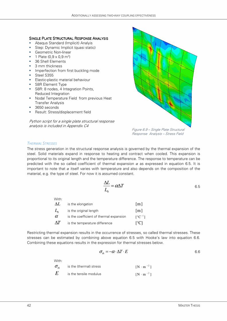
ADDITIONALLY ASSESSING TWO-WAY COUPLING EFFECTIVENESS
42 MASTER THESIS
SSSSINGLE INGLE INGLE INGLE PPPPLATE LATE LATE LATE SSSSTRUCTURAL TRUCTURAL TRUCTURAL TRUCTURAL RRRRESPONSEESPONSEESPONSEESPONSE AAAANALYSISNALYSISNALYSISNALYSIS
� Abaqus Standard (Implicit) Analyis
� Step: Dynamic Implicit (quasi static)
� Geometric Non-linear
� 1 Plate (0,9 x 0,9 m2)
� 36 Shell Elements
� 3 mm thickness
� Imperfection from first buckling mode
� Steel S355
� Elastic-plastic material behaviour
� S8R Element Type
� S8R: 8 nodes, 4 Integration Points,
Reduced Integration
� Nodal Temperature Field from previous Heat
Transfer Analysis
� 3650 seconds
� Result: Stress/displacement field
Python script for a single plate structural response analysis is included in Appendix C4
Figure 6.9 – Single Plate Structural Response Analysis – Stress Field
THERMAL STRESSES
The stress generation in the structural response analysis is governed by the thermal expansion of the
steel. Solid materials expand in response to heating and contract when cooled. This expansion is
proportional to its original length and the temperature difference. The response to temperature can be
predicted with the so called coefficient of thermal expansion N as expressed in equation 6.5. It is
important to note that N itself varies with temperature and also depends on the composition of the
material, e.g. the type of steel. For now it is assumed constant.
0
LT
Lα
∆= ∆ 6.5
With:
L∆ is the elongation [m]
0L is the original length [m]
α is the coefficient of thermal expansion 1[°C ]
−
T∆ is the temperature difference [°C]
Restricting thermal expansion results in the occurrence of stresses, so called thermal stresses. These
stresses can be estimated by combining above equation 6.5 with Hooke’s law into equation 6.6.
Combining these equations results in the expression for thermal stresses below.
th T Eσ α ⋅∆= − ⋅ 6.6
With:
thσ is the (thermal) stress 2[N m ]
−⋅
E is the tensile modulus 2[N m ]
−⋅
FDS-2-ABAQUS: C++ MANAGED AUTOMATED PYTHON SCRIPTED CFD-FEM COUPLING
J.A. FEENSTRA 43
For steel S355 N = 12 ∙ 10�O ℃��, ∆� = 500 ℃, and R = 210 ∙ 10S N ∙ m�5. The thermal stresses for the
one-dimensional case increase with 2,52 N ∙ mm�5°C��. To relax these thermal stresses the structure
tends to buckle (bend), effectively exchanging compressive thermal stresses for some bending
stresses.
When a material is compressed in one direction it often tends to expand in the other two directions.
This behaviour can be predicted using the so called Poisson’s ratio &. The Poisson’s ratio is the ratio of
transverse contraction strain to longitudinal extension strain in the direction of the stretching force.
Imagine a plate fixed on its top and bottom edge (Figure 6.3). If subjected to a fire the plate expands in
both directions, due to its boundary condition it cant expand to the top or bottom generating thermal
stresses. Restriction of (thermal) expansion in one direction will result in additional expansion in the
other direction (out-of-plane neglected). This additional expansion could, for instance when partly
restricted, generate additional (Poisson) stresses. Long story short: the relation between different strain
directions influence the stress behaviour.
trans
longitudinal
εν
ε= − 6.7
With:
ν is the Poisson’s ratio
transε is transverse strain
.longε is longitudinal strain
INTRODUCING IMPERFECTIONS
To accurately predict the structural response to the temperature increase an imperfection should be
introduced in the perfectly flat plate to allow out-of-plane bending. This imperfection is implemented as
a linear superposition of the first buckling eigenmode obtained from a separate buckling analyses. The
separate buckling analysis consist of the same structural model applying a linear perturbation buckle
step combined with a uniform normalized temperature field as the unit load. To capture the buckling
modes it is necessary to export result file (jobname.fil) containing the nodal displacements. This file
can be obtained by directly editing the input file (‘Model’ → ‘Edit Keyword’) and include the
following lines after **FIELD OUTPUT.
… *NODE FILE
U
…
To include it in a python script the following lines should be added.
… modKey = mdb.models['Model-1'].keywordBlock
modKey.synchVersions(storeNodesAndElements=False) modKey.insert(47, '\n*Node File\nU')
…
It is important to note that the python script imports a string at a certain line number. Therefore if the
model is developed further the required position for the additional lines requesting the result file could
change, and should be checked.

ADDITIONALLY ASSESSING TWO-WAY COUPLING EFFECTIVENESS
44 MASTER THESIS
To include the first eigenmode as imperfection in the structural response analysis the following lines
should be included in the input file. It is mandatory to enter the lines after **STEP.
… *IMPERFECTION, FILE=jobname, STEP=1
1, 0.005
…
The corresponding python commands are
… modKey = mdb.models['Model-1'].keywordBlock
modKey.synchVersions(storeNodesAndElements=False) modKey.insert(33,'\n*Imperfection, file=jobname, step=1\n1, 0.005')
…
Where jobname refers to the requested result file from the buckling analysis (tagged with the name
of the job in the buckling analysis). The values on the second line correspond to respectively the buckling
mode and the scale factor for the deflections. The eigenvector buckling modes are normalised to give
a maximum deflection of 1 unit.
An alternative method to introduce an imperfection is by drawing a slightly curved plate in the initial
creation of the part. For additional information on implementing a geometrical imperfection is referred
to the Abaqus Analyses User’s Guide 11.3.1 [34].
IMPORTING NODAL TEMPERATURE DATA
The output data from the Heat Transfer analysis can be directly read into the structural response
analysis. Nodal temperatures (NT) are stored as function of time in the heat transfer analyses output
database file. The temperature distributions can be input directly into the stress analysis as a predefined
field, at the nodes, and interpolated to the calculations points within the elements as needed. Abaqus
even allows the use of dissimilar meshes for both analyses. The temperature values will be interpolated
based on element interpolators evaluated at nodes of the thermal-stress model. To import the
temperature data from the HeatTranfer.odb file into the structural response analysis the following
lines should be added.
… mdb.models['Model-1'].Temperature(absoluteExteriorTolerance=0.0, beginIncrement=None, beginStep=None, createStepName='i0-SR-Step', distributionType=FROM_FILE, endIncrement=None, endStep=None, exteriorTolerance=0.05, fileName='path\HeatTranfer.odb',
interpolate=ON, name='Temp-From-HT')
…
For additional reading on the (sequentially) coupled thermal-stress analyses in Abaqus is referred to the
Abaqus Analysis User's Guide sections 16.1.2 [33].

FDS-2-ABAQUS: C++ MANAGED AUTOMATED PYTHON SCRIPTED CFD-FEM COUPLING
J.A. FEENSTRA 45
6.5 MULTIPLE PLATE MODELS
This section discusses how to extend the previous models
to include multiple instances of a single part. Additionally the
use of thermal and structural tie constraints between the
plate-instances is addressed. The numbering convention for
both plates and temperature partitions is from bottom to top
first and from left to right second. This numbering
convention is illustrated in the typical SR output in Figure
6.10.
MULTIPLE PLATE-INSTANCES MODEL
As previously discussed in section 6.2 an Abaqus model
consist of one assembly consisting of a single or multiple
instance(s) of one or several parts. Therefore the single
plate-instance model, as discussed in the previous sections,
can be easily expanded to include multiple plate-instances
of the same part. Various geometric operations for
instances are included in Abaqus like translation, rotation
and linear and radial patterns. As an example the following
lines create a 2x2 plate-pattern.
… modRa = mdb.models['Model-1'].rootAssembly modRa.LinearInstancePattern(instanceList=('Plate-1', ), direction1=(1.0, 0.0, 0.0), direction2=(0.0, 1.0, 0.0), number1=2, number2=2, spacing1=0.9, spacing2=0.9)
…
Abaqus automatically assigns names to the newly generated plate-instances based on their original
name and their location in the pattern. To rename these instances the following lines should be added.
… modRaFe = modRa.features
modRaFe.changeKey(fromName='Plate-1-lin-1-2', toName='Plate-2')
modRaFe.changeKey(fromName='Plate-1-lin-2-1', toName='Plate-3') modRaFe.changeKey(fromName='Plate-1-lin-2-2', toName='Plate-4') …
Since Abaqus generates multiple instances of the same part all previous and possible newly assigned
SETS and SURFACES in the part are automatically created for all instances. The plate-instances are
structurally and thermally independent. Depending on the modelled structural system, structural and/or
thermal ties could be implemented. The tying of instances is discussed in the next section.
Figure 6.10 – Numbering convention overlay on a 12 (untied) plate-instance Abaqus SR model with each plate subdivided into 36 finite elements
ADDITIONALLY ASSESSING TWO-WAY COUPLING EFFECTIVENESS
46 MASTER THESIS
TYING PLATES
Plate-instances can be tied using TIE constraints. A TIE constraint ties two separate surfaces together
so that there is no relative motion between them, effectively fusing them together. To define a TIE
constraint a master and slave surface should be selected. As an example the following lines tie together
Plate-1 and Plate-2.
… mod = mdb.models['Model-1']
mod.Tie(name='Tie_P1-P2',
master=modRa.instances['Plate-1'].surfaces['Surf-0'], slave=modRa.instances['Plate-2'].surfaces['Surf-0']) …
Alternatively the plates can be tied by selecting edges or node regions. Although this does not work for
the Heat Transfer Analysis which has to use the surface method listed above. Specific edges can be
tied using the following lines.
… mod.Tie(name='Tie_P1-P2',
master=modRa.instances['Plate-1'].sets['Edge-Top'],
slave=modRa.instances['Plate-2'].sets['Edge-Bot']) …
The slave nodes degrees of freedom (dof) are written as a linear combination of master dofs in a
constraint equation. If slave nodes are defined in more than one constraint equation this can result in
over-constrained nodes thereby obtaining questionable results. Abaqus does warn for, and often
deactivates, over-constrained nodes.
The combination of ties with the restart analysis and plate removal has proved challenging for additional
reading on this challenge is referred to section 8.2. For additional information on TIE constraints is
referred to the Abaqus/CAE User’s Guide 15.15.1 [33].
SINGLE PART INSTANCE MODEL
An alternative approach to a structural system consisting of multiple plates is to define the system as
a single part and assign subsection as plate-area’s. Either by redrawing the complete system as a single
plate or, alternatively, by merging the meshes of the plate-instances of the ‘multiple-plate-instances’
approach. When using this method Abaqus will supress all part-instances and create a new part
instance with all instances combined. The major drawback of this method is that all SET and SURFACE
information is lost and needs to be reassigned.
The major advantage for this approach is, given only a single ‘full-wall’ part is defined, that all plates are
automatically tied and no additional TIE-constraints need to be defined. The major drawback for this
approach is that for every plate all plate SETS and (temperature partition) SURFACES need to be defined
individually.
6.6 RESTART ANALYSIS
In order to restart or continue any simulation a restart file *.fil should be requested in the step
module. One can either define a frequency U or interval to control restart file creation. For frequency
U restart data is written every n’th increment (and the last). For interval , the step is divided into
intervals and restart data is written at the end of every interval, if time marks is checked restart data
will be written for the increment closest to this interval. The Boolean argument overlay specifies that
restart data should be overwritten, thereby minimizing the size of the restart file. As an example the
following lines request a restart file at the end of the step (single interval).

FDS-2-ABAQUS: C++ MANAGED AUTOMATED PYTHON SCRIPTED CFD-FEM COUPLING
J.A. FEENSTRA 47
… mod = mdb.models['Model-1']
mod.steps['i0_SR-Step'].Restart(frequency=0, numberIntervals=1,
overlay=ON, timeMarks=OFF) …
In the subsequent analysis this restart data should be specified to allow Abaqus to restart from the
previous simulation. As illustrated in the following lines.
… mod = mdb.models['Model-1'] mod.setValues(restartJob='i0_SR-Job', restartStep='i0_SR-Step') …
In addition the job type needs to be set to restart, compared to the standard full analysis. The restart
job type is automatically selected when creating a job in Abaqus CAE but needs to be specified when
using python script input. An example is found in the following line.
… mdb.Job(name='i1_SR-Job', model='Model-1', type=RESTART) …
For additional information on restart simulations is referred to the Abaqus Analysis Guide section 9.1.1
[33].
6.7 REMOVING PLATES
Plates can be removed from the simulation by a model change interaction from the interaction module.
The model change interaction can be used to deactivate, or reactivate) a region in the model. Both
geometry and element regions can be deactivated. A model change interaction can only be defined at
the beginning of a (restart) step. As an example the following lines deactivate the geometry region
Plate-Area for instance Plate-2 at the beginning of step i1_SR-Step.
… mod = mdb.models['Model-1'] thisPlate = mod.rootAssembly.instances['Plate-2'].sets['Plate-Area'] mod.ModelChange(activeInStep=False, createStepName='i1_SR-Step', includeStrain=False, name='deActPlate-2', region=thisPlate)
…
Using a model change interaction in a restart analysis is only possible if a model change interaction was
defined in the original model. To include the model change interaction in the initial model the following
lines should be included.
… mod.ModelChange(name='ModelChange', createStepName='i0_SR-Step',
isRestart=True) …
For additional information on the model change interaction is referred to the Abaqus/CAE User’s Guide
section 15.3.3 [33].

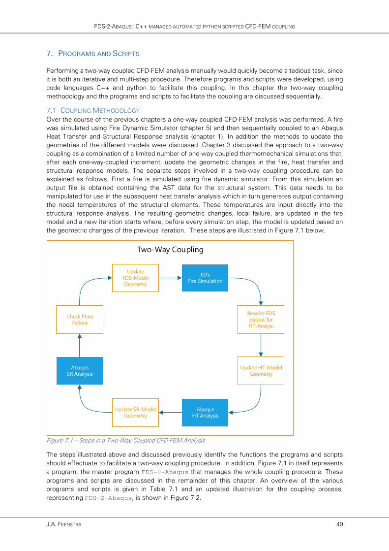
FDS-2-ABAQUS: C++ MANAGED AUTOMATED PYTHON SCRIPTED CFD-FEM COUPLING
J.A. FEENSTRA 49
7. PROGRAMS AND SCRIPTS
Performing a two-way coupled CFD-FEM analysis manually would quickly become a tedious task, since
it is both an iterative and multi-step procedure. Therefore programs and scripts were developed, using
code languages C++ and python to facilitate this coupling. In this chapter the two-way coupling
methodology and the programs and scripts to facilitate the coupling are discussed sequentially.
7.1 COUPLING METHODOLOGY
Over the course of the previous chapters a one-way coupled CFD-FEM analysis was performed. A fire
was simulated using Fire Dynamic Simulator (chapter 5) and then sequentially coupled to an Abaqus
Heat Transfer and Structural Response analysis (chapter 1). In addition the methods to update the
geometries of the different models were discussed. Chapter 3 discussed the approach to a two-way
coupling as a combination of a limited number of one-way coupled thermomechanical simulations that,
after each one-way-coupled increment, update the geometric changes in the fire, heat transfer and
structural response models. The separate steps involved in a two-way coupling procedure can be
explained as follows. First a fire is simulated using fire dynamic simulator. From this simulation an
output file is obtained containing the AST data for the structural system. This data needs to be
manipulated for use in the subsequent heat transfer analysis which in turn generates output containing
the nodal temperatures of the structural elements. These temperatures are input directly into the
structural response analysis. The resulting geometric changes, local failure, are updated in the fire
model and a new iteration starts where, before every simulation step, the model is updated based on
the geometric changes of the previous iteration. These steps are illustrated in Figure 7.1 below.
FDSFire Simulation
AbaqusHT Analysis
AbaqusSR Analysis
upGeomFDS
upGeomHT
upGeomSR
reWriteAST2pyPlateFailureCheck
Two-Way Coupling
Rewrite FDS output for HT-Analysi
Update HT-ModelGeometry
Update SR-ModelGeometry
Check PlateFailure
Update FDS-ModelGeometry
Figure 7.1 – Steps in a Two-Way Coupled CFD-FEM Analysis
The steps illustrated above and discussed previously identify the functions the programs and scripts
should effectuate to facilitate a two-way coupling procedure. In addition, Figure 7.1 in itself represents
a program, the master program FDS-2-Abaqus that manages the whole coupling procedure. These
programs and scripts are discussed in the remainder of this chapter. An overview of the various
programs and scripts is given in Table 7.1 and an updated illustration for the coupling process,
representing FDS-2-Abaqus, is shown in Figure 7.2.

ADDITIONALLY ASSESSING TWO-WAY COUPLING EFFECTIVENESS
50 MASTER THESIS
Table 7.1 – Overview of programs and scripts to facilitate two-way coupling procedure
PPPPROGRAMME ROGRAMME ROGRAMME ROGRAMME //// SSSSCRIPTCRIPTCRIPTCRIPT DDDDESCRIPTIONESCRIPTIONESCRIPTIONESCRIPTION FDS-2-Abaqus Master Programme – managing two-way coupling procedure upGeomFDS Updates FDS input file for current iteration reWriteAST2py Rewrites AST data for use in subsequent HT analysis upGeomHT Updates HT script for current iteration upGeomSR Updates SR script for current iteration PlateFailureCheck Checks SR output for possible plate failure
FDSFire Simulation
AbaqusHT Analysis
AbaqusSR Analysis
upGeomFDS
upGeomHT
upGeomSR
reWriteAST2pyPlateFailureCheck
__ __ __ __
|_ | \(_ __ _) __ /\ |_ _ _ _
| |__/__) /__ /--\|_)(_|(_||_|_)
|
Figure 7.2 – Core process of coupling methodology as managed by Master programme FDS-2-Abaqus
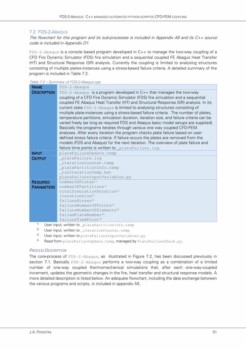
FDS-2-ABAQUS: C++ MANAGED AUTOMATED PYTHON SCRIPTED CFD-FEM COUPLING
J.A. FEENSTRA 51
7.2 FDS-2-ABAQUS
The flowchart for this program and its sub-processes is included in Appendix A5 and its C++ source
code is included in Appendix D1.
FDS-2-Abaqus is a console based program developed in C++ to manage the two-way coupling of a
CFD Fire Dynamic Simulator (FDS) fire simulation and a sequential coupled FE Abagus Heat Transfer
(HT) and Structural Response (SR) analysis. Currently the coupling is limited to analysing structures
consisting of multiple plates-instances using a stress-based failure criteria. A detailed summary of the
program is included in Table 7.2.
Table 7.2 – Summary of FDS-2-Abaqus.cpp
NNNNAMEAMEAMEAME FDS-2-Abaqus
DDDDESCRIPTIONESCRIPTIONESCRIPTIONESCRIPTION FDS-2-Abaqus is a program developed in C++ that manages the two-way
coupling of a CFD Fire Dynamic Simulator (FDS) fire simulation and a sequential
coupled FE Abaqus Heat Transfer (HT) and Structural Response (SR) analysis. In its
current state FDS-2-Abaqus is limited to analysing structures consisting of
multiple plate-instances using a stress-based failure criteria. The number of plates,
temperature partitions, simulation duration, iteration size, and failure criteria can be
varied freely (as long as required FDS and Abaqus basic model setups are supplied).
Basically the programs iterates through various one way coupled CFD-FEM
analyses. After every iteration the program checks plate failure based on user-
defined stress failure criteria. If failure occurs the plates are removed from the
models (FDS and Abaqus) for the next iteration. The overview of plate failure and
failure time points is written to _plateFailure.log.
IIIINPUTNPUTNPUTNPUT plateFailureUpdate.temp
OOOOUTPUTUTPUTUTPUTUTPUT _plateFailure.log
_iterationCounter.temp
_platePartitionInfo.temp
_runIterationTemp.bat
plateFailureInputVariables.py
RRRREQUIRED EQUIRED EQUIRED EQUIRED
PPPPARAMETERSARAMETERSARAMETERSARAMETERS
numberOfPlates1)
numberOfPartitions1)
totalSimulationDuration2)
iterationSize2)
failureStress3)
failureNumberOfPoints3)
failureNumberOfElements3)
failedPlateNumber4)
failureTimePoint4)
1) User input, written to _platePartitionInfo.temp
2) User input, written to _iterationCounter.temp
3) User input, written to plateFailureInputVariables.py 4) Read from plateFailureUpdate.temp, managed by PlateFailureCheck.py.
PROCESS DESCRIPTION
The core-process of FDS-2-Abaqus, as illustrated in Figure 7.2, has been discussed previously in
section 7.1. Basically FDS-2-Abaqus performs a two-way coupling as a combination of a limited
number of one-way coupled thermomechanical simulations that, after each one-way-coupled
increment, updates the geometric changes in the fire, heat transfer and structural response models. A
more detailed description is listed below. An adequate flowchart, including the data exchange between
the various programs and scripts, is included in appendix A5.

ADDITIONALLY ASSESSING TWO-WAY COUPLING EFFECTIVENESS
52 MASTER THESIS
� Check existence of required files.
� Request basic variables (console input)
� Create plateFailureArray to log plate failure progression.
� Create data files _plateFailure.log, platePartitionInfo.temp.
� Create iteration batch file _runIterationTemp.bat containing the actual coupling
sequence as listed (see Figure 7.2):
� Run upGeomFDS.exe
� Run FDS_Simulation
� Run reWriteAST2py.exe
� Run upGeomHT.exe
� Run Abaqus HT simulation
� Run upGeomSR.exe
� Run Abaqus SR simulation
� Run PlateFailureCheck.py
� While loop consisting of the following sequence (continues running till
totalSimulationDuration is reached):
� Write/update current iteration info to data file _iterationCounter.temp.
� Write/update failure criteria and paths to data script
plateFailureInputVariables.py.
� Run _runIterationTemp.bat (see above).
� Update plateFailureArray based on plateFailureUpdate.temp.
� Next iteration
� Output completion info and summarize results
The C++ source code for this program is included in Appendix D1. This source code includes
extensive comments for code clarification.
USING FDS-2-ABAQUS
In order to perform a two-way coupled
analysis using FDS-2-Abaqus the
following steps should be followed.
� Run FDS-2-Abaqus
� Supply necessary files
� Specify basic variables
� Specify failure Criteria
� Verify input and run simulation
� Check output for possible errors
The FDS-2-Abaqus interface, as
illustrated in Figure 7.3, will guide the user
through the above process. For the sake of
completeness an overview of all
necessary files and folders is included in
Table 7.3.
Both FDS and Abaqus need to be installed on the computer before running FDS-2-Abaqus. A detailed
installation guide is included in appendix E1. In addition a worked example is included in appendix E2.
Lastly a debug guide is included in appendix E3.
Figure 7.3 - FDS-2-Abaqus Console Interface
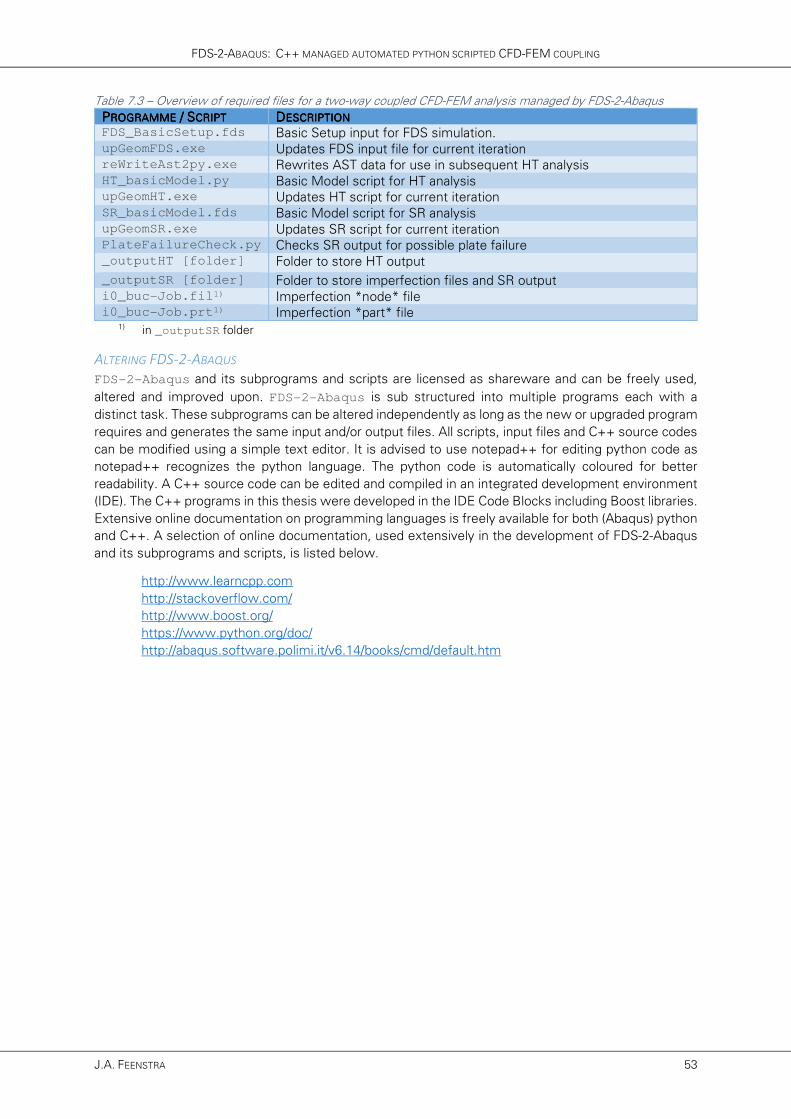
FDS-2-ABAQUS: C++ MANAGED AUTOMATED PYTHON SCRIPTED CFD-FEM COUPLING
J.A. FEENSTRA 53
Table 7.3 – Overview of required files for a two-way coupled CFD-FEM analysis managed by FDS-2-Abaqus
PPPPROGRAMME ROGRAMME ROGRAMME ROGRAMME //// SSSSCRIPTCRIPTCRIPTCRIPT DDDDESCRIPTIONESCRIPTIONESCRIPTIONESCRIPTION FDS_BasicSetup.fds Basic Setup input for FDS simulation. upGeomFDS.exe Updates FDS input file for current iteration reWriteAst2py.exe Rewrites AST data for use in subsequent HT analysis HT_basicModel.py Basic Model script for HT analysis upGeomHT.exe Updates HT script for current iteration SR_basicModel.fds Basic Model script for SR analysis upGeomSR.exe Updates SR script for current iteration PlateFailureCheck.py Checks SR output for possible plate failure _outputHT [folder] Folder to store HT output
_outputSR [folder] Folder to store imperfection files and SR output i0_buc-Job.fil1) Imperfection *node* file i0_buc-Job.prt1) Imperfection *part* file
1) in _outputSR folder
ALTERING FDS-2-ABAQUS
FDS-2-Abaqus and its subprograms and scripts are licensed as shareware and can be freely used,
altered and improved upon. FDS-2-Abaqus is sub structured into multiple programs each with a
distinct task. These subprograms can be altered independently as long as the new or upgraded program
requires and generates the same input and/or output files. All scripts, input files and C++ source codes
can be modified using a simple text editor. It is advised to use notepad++ for editing python code as
notepad++ recognizes the python language. The python code is automatically coloured for better
readability. A C++ source code can be edited and compiled in an integrated development environment
(IDE). The C++ programs in this thesis were developed in the IDE Code Blocks including Boost libraries.
Extensive online documentation on programming languages is freely available for both (Abaqus) python
and C++. A selection of online documentation, used extensively in the development of FDS-2-Abaqus
and its subprograms and scripts, is listed below.
http://www.learncpp.com
http://stackoverflow.com/
http://www.boost.org/
https://www.python.org/doc/
http://abaqus.software.polimi.it/v6.14/books/cmd/default.htm
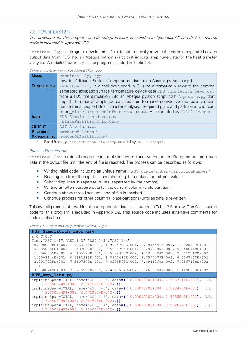
ADDITIONALLY ASSESSING TWO-WAY COUPLING EFFECTIVENESS
54 MASTER THESIS
7.3 REWRITEAST2PY
The flowchart for this program and its sub-processes is included in Appendix A3 and its C++ source
code is included in Appendix D2.
ReWriteAST2py is a program developed in C++ to automatically rewrite the comma separated device
output data from FDS into an Abaqus python script that imports amplitude data for the heat transfer
analysis. A detailed summary of the program is listed in Table 7.4.
Table 7.4 – Summary of reWriteAST2py.cpp
NNNNAMEAMEAMEAME reWriteAST2py.cpp
[rewrite Adiabatic Surface Temperature data to an Abaqus python script]
DDDDESCRIPTIONESCRIPTIONESCRIPTIONESCRIPTION reWriteAST2py is a tool developed in C++ to automatically rewrite the comma
separated adiabatic surface temperature device data FDS_Simulation_devc.csv
from a FDS fire simulation into an Abaqus python script AST_Amp_data.py that
imports the tabular amplitude data required to model convective and radiative heat
transfer in a coupled Heat Transfer analysis. Required plate and partition info is read
from _platePartitionInfo.temp a temporary file created by FDS-2-Abaqus.
IIIINPUTNPUTNPUTNPUT FDS_Simulation_devc.csv
_platePartitionInfo.temp
OOOOUTPUTUTPUTUTPUTUTPUT AST_Amp_Data.py
RRRREQUIRED EQUIRED EQUIRED EQUIRED
PPPPARAMETERSARAMETERSARAMETERSARAMETERS
numberOfPlates1)
numberOfPartitions1) 1) Read from _platePartitionInfo.temp, created by FDS-2-Abaqus.
PROCESS DESCRIPTION
reWriteAST2py iterates through the input file line by line and writes the time/temperature amplitude
data in the output file until the end of file is reached. The process can be described as follows:
� Writing initial code including an unique name, ‘AST_plateNumber-partitionNumber’
� Reading line from the input file and checking if it contains time/temp value’s
� Subdividing lines in separate values (separated by the comma)
� Writing time/temperature data for the current column (plate-partition)
� Continue above three lines until end of file is reached
� Continue process for other columns (plate-partitions) until all data is rewritten
This overall process of rewriting the temperature data is illustrated in Table 7.5 below. The C++ source
code for this program is included in Appendix D2. This source code includes extensive comments for
code clarification.
Table 7.5 – input and output of reWriteAST2py
FDS_Simulation_devc.csv s,C,C,C,C
Time,"AST_1-1","AST_1-2","AST_1-3","AST_1-4"
0.0000000E+000, 1.9933111E+001, 1.9924704E+001, 1.9935541E+001, 1.9926727E+001
5.0350356E+000, 1.2587006E+002, 9.5066795E+001, 1.2907686E+002, 9.6406448E+001
1.0006359E+001, 4.5135278E+002, 3.6574329E+002, 4.6353320E+002, 3.8612912E+002
1.5002146E+001, 6.5682263E+002, 6.0171484E+002, 6.7507477E+002, 6.0263403E+002
2.0017225E+001, 7.3107379E+002, 7.0298578E+002, 7.4941260E+002, 7.2567188E+002
[…]
3.6500249E+003, 2.3215961E+002, 2.4729654E+002, 2.2615050E+002, 2.4190033E+002 AST_Amp_Data.py imp(timeSpan=TOTAL, name='AST_1-1', data=(( 0.0000000E+000, 1.9933111E+001), […],
( 3.6500249E+003, 2.3215961E+002),)) imp(timeSpan=TOTAL, name='AST_1-2', data=(( 0.0000000E+000, 1.9924704E+001), […],
( 3.6500249E+003, 2.4729654E+002),)) imp(timeSpan=TOTAL, name='AST_1-3', data=(( 0.0000000E+000, 1.9935541E+001), […],
( 3.6500249E+003, 2.2615050E+002),)) imp(timeSpan=TOTAL, name='AST_1-4', data=(( 0.0000000E+000, 1.9926727E+001), […],
( 3.6500249E+003, 2.4190033E+002),))

FDS-2-ABAQUS: C++ MANAGED AUTOMATED PYTHON SCRIPTED CFD-FEM COUPLING
J.A. FEENSTRA 55
The resulting output script can be called from the heat transfer analysis by including the following lines
in the python script for the heat transfer analysis.
… imp = mdb.models['Model'].TabularAmplitude execfile('path\AST_Amp_Data.py', __main__.__dict__)
…

ADDITIONALLY ASSESSING TWO-WAY COUPLING EFFECTIVENESS
56 MASTER THESIS
7.4 UPGEOMFDS
The C++ source code for this program is included in Appendix D3.
upGeomFDS is a program developed in C++ to automatically update a basic FDS input file for the current
iteration. A detailed summary of the program is listed in Table 7.6.
Table 7.6 – Summary of upGeomFDS.cpp
NNNNAMEAMEAMEAME upGeomFDS.cpp
[update Geometry Fire Dynamic Simulator (model)]
DDDDESCRIPTIONESCRIPTIONESCRIPTIONESCRIPTION upGeomFDS is a program developed in C++ that creates a FDS input file for the
current iteration. Basically it copies the basicSetupFile, FDS_BasicSetup.fds, to a
new input file, FDS_Script.fds, and appends input lines defining the next
iteration and plate failure devices. The iteration parameters are read from temporary
file _iterationCounter.temp and the plate failure parameters from
_plateFailure.log. Both of which are managed by the ‘Master program’
FDS-2-Abaqus.
IIIINPUTNPUTNPUTNPUT FDS_BasicSetup.fds3)
_iterationCounter.temp
_plateFailure.log
_platePartitionInfo.temp
OOOOUTPUTUTPUTUTPUTUTPUT FDS_Script.fds
RRRREQUIRED EQUIRED EQUIRED EQUIRED
PPPPARAARAARAARAMETERSMETERSMETERSMETERS
iterationCounter1)
iterationSize1)
totalSimulationDuration1)
failedPlateNumber2)
failureTimePoint2)
plateFailureBool2) 1) Read from _iterationCounter.temp, managed by FDS-2-Abaqus.
2) Read from _plateFailure.log, managed by FDS-2-Abaqus. 3) Should be supplied by user!
PROCESS DESCRIPTION
upGeomFDS copies the basicSetupFile FDS_BasicSetup.fds to a new input file and appends
additional input lines controlling the duration of the next iteration and the removal of failed plates. The
process can be described as follows:
� Read current iteration from _iterationCounter.temp.
� Read number of plates and partitions from _platePartitionInfo.temp.
� Copy basic setup FDS input file FDS_BasicSetup.fds to new input file FDS_Script.fds.
� Append RESTART and KILL lines for current iteration (see section 5.3)
� Read plate(failure) info from _plateFailure.log.
� Append input lines controlling (possible) plate removal based on _plateFailure.log
(see section 5.3).
� Write &TAIL input line and finalize script.
The C++ source code for this program is included in Appendix D3. This source code includes
extensive comments for code clarification.
upGeomFDS is managed by master program FDS-2-Abaqus meaning its required parameters are read
from the data files created by FDS-2-Abaqus. It is very important to note that a valid
FDS_BasicSetup.fds input file should be supplied by the USER to create a functioning (updated)
FDS input file and subsequently perform a coupled analysis. An example of an FDS_BasicSetup.fds
input file for an office with a 12-plate façade is included in Appendix B2. An example of typical code
appended by the upGeomFDS program is included in Appendix B3. The C++ source code for this
program is included in Appendix D3. This source code includes extensive comments for code
clarification.

FDS-2-ABAQUS: C++ MANAGED AUTOMATED PYTHON SCRIPTED CFD-FEM COUPLING
J.A. FEENSTRA 57
7.5 UPGEOMHT
The C++ source code for this program is included in Appendix D4.
upGeomHT is a program developed in C++ to automatically update the basic Abaqus python script for
the Heat Transfer analysis for the current iteration. A detailed summary of the program is listed in Table
7.7.
Table 7.7 – Summary of upGeomHT.cpp
NNNNAMEAMEAMEAME upGeomHT.cpp
[update Geometry Heat Transfer (Analysis)]
DDDDESCRIPTIONESCRIPTIONESCRIPTIONESCRIPTION upGeomHT is a program developed in C++ that creates an Abaqus Heat Transfer (HT)
python script for the current iteration. Basically it copies the basic model setup,
HT_basicModel.py, to a new python script, HT_Script.py, and appends
additional python code to update step, restart, AST, heat transfer and geometry info
for the current iteration. The AST amplitude script AST_Amp_data.py, which is
generated by the reWriteAST2py program, is used to update the AST data.
Required iteration parameters are read from temporary file
_iterationCounter.temp, the plate and partition parameters are read from
_platePartitionInfo.temp, and plate failure parameters from
_plateFailure.log. All of which are managed by the ‘Master program’
FDS-2-Abaqus.
IIIINPUTNPUTNPUTNPUT HT_basicModel.py
_iterationCounter.temp
_platePartitionInfo.temp
_plateFailure.log
AST_Amp_data.py
OOOOUTPUTUTPUTUTPUTUTPUT HT_Script.py
ix_Script.py
RRRREQUIRED EQUIRED EQUIRED EQUIRED
PPPPARAMETERSARAMETERSARAMETERSARAMETERS
iterationCounter1)
iterationSize1)
totalSimulationDuration1)
numberOfPlates2)
numberOfPartitions2)
failedPlateNumber3)
failureTimePoint3)
plateFailureBool3) 1) Read from _iterationCounter.temp, managed by FDS-2-Abaqus.
2) Read from _platePartitionInfo.temp, managed by FDS-2-Abaqus. 3) Read from _plateFailure.log, managed by FDS-2-Abaqus.
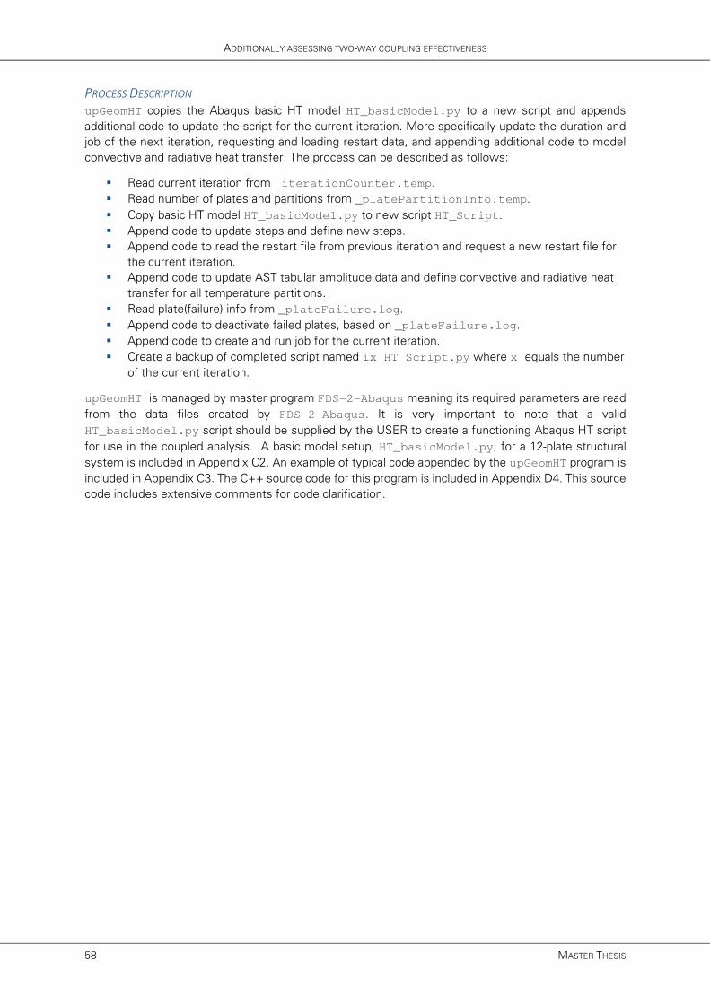
ADDITIONALLY ASSESSING TWO-WAY COUPLING EFFECTIVENESS
58 MASTER THESIS
PROCESS DESCRIPTION
upGeomHT copies the Abaqus basic HT model HT_basicModel.py to a new script and appends
additional code to update the script for the current iteration. More specifically update the duration and
job of the next iteration, requesting and loading restart data, and appending additional code to model
convective and radiative heat transfer. The process can be described as follows:
� Read current iteration from _iterationCounter.temp.
� Read number of plates and partitions from _platePartitionInfo.temp.
� Copy basic HT model HT_basicModel.py to new script HT_Script.
� Append code to update steps and define new steps.
� Append code to read the restart file from previous iteration and request a new restart file for
the current iteration.
� Append code to update AST tabular amplitude data and define convective and radiative heat
transfer for all temperature partitions.
� Read plate(failure) info from _plateFailure.log.
� Append code to deactivate failed plates, based on _plateFailure.log.
� Append code to create and run job for the current iteration.
� Create a backup of completed script named ix_HT_Script.py where x equals the number
of the current iteration.
upGeomHT is managed by master program FDS-2-Abaqus meaning its required parameters are read
from the data files created by FDS-2-Abaqus. It is very important to note that a valid
HT_basicModel.py script should be supplied by the USER to create a functioning Abaqus HT script
for use in the coupled analysis. A basic model setup, HT_basicModel.py, for a 12-plate structural
system is included in Appendix C2. An example of typical code appended by the upGeomHT program is
included in Appendix C3. The C++ source code for this program is included in Appendix D4. This source
code includes extensive comments for code clarification.
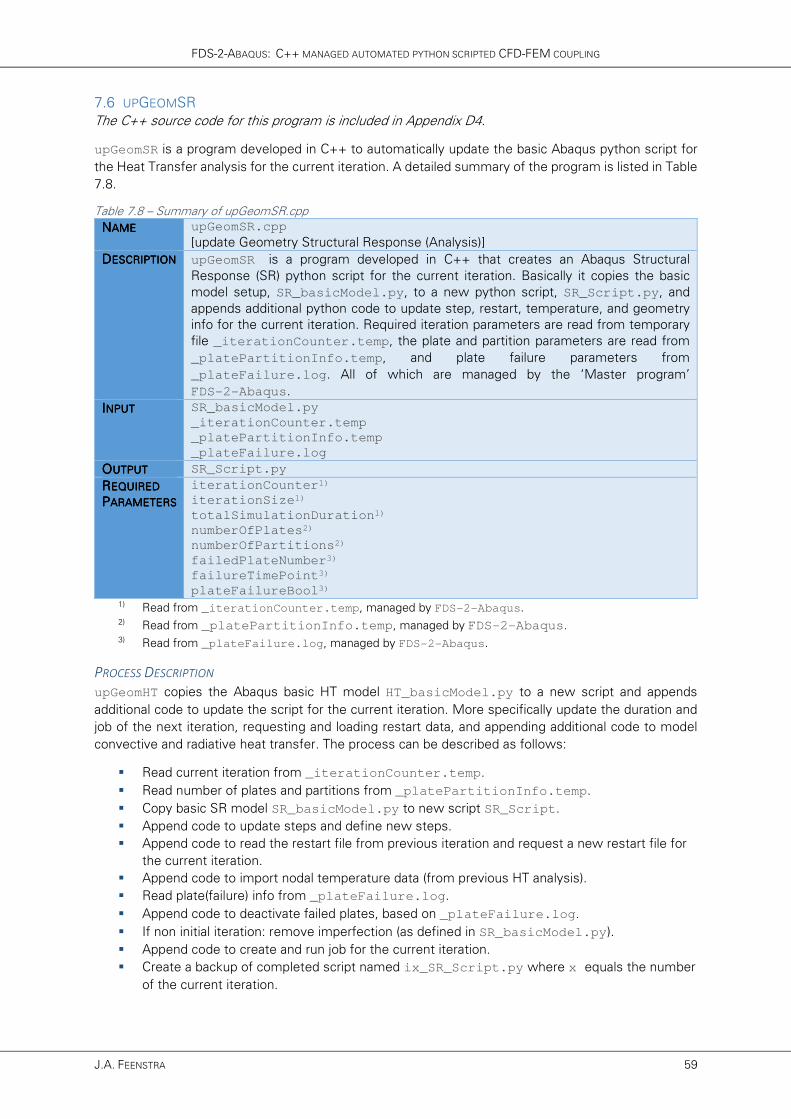
FDS-2-ABAQUS: C++ MANAGED AUTOMATED PYTHON SCRIPTED CFD-FEM COUPLING
J.A. FEENSTRA 59
7.6 UPGEOMSR
The C++ source code for this program is included in Appendix D4.
upGeomSR is a program developed in C++ to automatically update the basic Abaqus python script for
the Heat Transfer analysis for the current iteration. A detailed summary of the program is listed in Table
7.8.
Table 7.8 – Summary of upGeomSR.cpp
NNNNAMEAMEAMEAME upGeomSR.cpp
[update Geometry Structural Response (Analysis)]
DDDDESCRIPTIONESCRIPTIONESCRIPTIONESCRIPTION upGeomSR is a program developed in C++ that creates an Abaqus Structural
Response (SR) python script for the current iteration. Basically it copies the basic
model setup, SR_basicModel.py, to a new python script, SR_Script.py, and
appends additional python code to update step, restart, temperature, and geometry
info for the current iteration. Required iteration parameters are read from temporary
file _iterationCounter.temp, the plate and partition parameters are read from
_platePartitionInfo.temp, and plate failure parameters from
_plateFailure.log. All of which are managed by the ‘Master program’
FDS-2-Abaqus.
IIIINPUTNPUTNPUTNPUT SR_basicModel.py
_iterationCounter.temp
_platePartitionInfo.temp
_plateFailure.log
OOOOUTPUTUTPUTUTPUTUTPUT SR_Script.py
RRRREQUIRED EQUIRED EQUIRED EQUIRED
PPPPARAMETERSARAMETERSARAMETERSARAMETERS
iterationCounter1)
iterationSize1)
totalSimulationDuration1)
numberOfPlates2)
numberOfPartitions2)
failedPlateNumber3)
failureTimePoint3)
plateFailureBool3) 1) Read from _iterationCounter.temp, managed by FDS-2-Abaqus.
2) Read from _platePartitionInfo.temp, managed by FDS-2-Abaqus. 3) Read from _plateFailure.log, managed by FDS-2-Abaqus.
PROCESS DESCRIPTION
upGeomHT copies the Abaqus basic HT model HT_basicModel.py to a new script and appends
additional code to update the script for the current iteration. More specifically update the duration and
job of the next iteration, requesting and loading restart data, and appending additional code to model
convective and radiative heat transfer. The process can be described as follows:
� Read current iteration from _iterationCounter.temp.
� Read number of plates and partitions from _platePartitionInfo.temp.
� Copy basic SR model SR_basicModel.py to new script SR_Script.
� Append code to update steps and define new steps.
� Append code to read the restart file from previous iteration and request a new restart file for
the current iteration.
� Append code to import nodal temperature data (from previous HT analysis).
� Read plate(failure) info from _plateFailure.log.
� Append code to deactivate failed plates, based on _plateFailure.log.
� If non initial iteration: remove imperfection (as defined in SR_basicModel.py).
� Append code to create and run job for the current iteration.
� Create a backup of completed script named ix_SR_Script.py where x equals the number
of the current iteration.

ADDITIONALLY ASSESSING TWO-WAY COUPLING EFFECTIVENESS
60 MASTER THESIS
upGeomSR is managed by master program FDS-2-Abaqus meaning its required parameters are read
from the data files created by FDS-2-Abaqus. It is very important to note that a valid
SR_basicModel.py script should be supplied by the USER to create a functioning Abaqus SR script
for use in the coupling analysis. A basic model setup, SR_basicModel.py, for a 12-plate structural
system is included in Appendix C5. An example of typical code appended by the upGeomHT program is
included in Appendix C6. The C++ source code for this program is included in Appendix D5. This source
code includes extensive comments for code clarification.
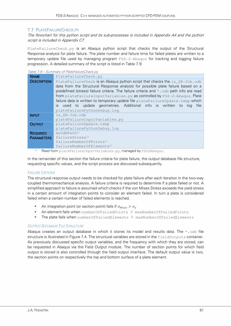
FDS-2-ABAQUS: C++ MANAGED AUTOMATED PYTHON SCRIPTED CFD-FEM COUPLING
J.A. FEENSTRA 61
7.7 PLATEFAILURECHECK.PY
The flowchart for this python script and its sub-processes is included in Appendix A4 and the python
script is included in Appendix C7
PlateFailureCheck.py is an Abaqus python script that checks the output of the Structural
Response analysis for plate failure. The plate number and failure time for failed plates are written to a
temporary update file used by managing program FDS-2-Abaqus for tracking and logging failure
progression. A detailed summary of the script is listed in Table 7.9.
Table 7.9 – Summary of PlateFailureCheck.py
NNNNAMEAMEAMEAME PlateFailureCheck.py
DDDDESCRIPTIONESCRIPTIONESCRIPTIONESCRIPTION PlateFailureCheck is an Abaqus python script that checks the ix_SR-Job.odb
data from the Structural Response analysis for possible plate failure based on a
predefined (stress) failure criteria. The failure criteria and *.odb path info are read
from plateFailureInputVariables.py as controlled by FDS-2-Abaqus. Plate
failure data is written to temporary update file plateFailureUpdate.temp which
is used to update geometries. Additional info is written to log file
plateFailurePythonDebug.log.
IIIINPUTNPUTNPUTNPUT ix_SR-Job.odb
plateFailureInputVariables.py
OOOOUTPUTUTPUTUTPUTUTPUT plateFailureUpdate.temp
plateFailurePythonDebug.log
RRRREQUIRED EQUIRED EQUIRED EQUIRED
PPPPARAMETERSARAMETERSARAMETERSARAMETERS
myOdbPath1)
failureStress1)
failureNumberOfPoints1)
failureNumberOfElements1) 1) Read from plateFailureInputVariables.py, managed by FDS2Abaqus.
In the remainder of this section the failure criteria for plate failure, the output database file structure,
requesting specific values, and the script process are discussed subsequently.
FAILURE CRITERIA
The structural response output needs to be checked for plate failure after each iteration in the two-way
coupled thermomechanical analysis. A failure criteria is required to determine if a plate failed or not. A
simplified approach to failure is assumed which checks if the von Mises Stress exceeds the yield stress
in a certain amount of integration points to consider an element failed. In turn a plate is considered
failed when a certain number of failed elements is reached.
� An integration point (or section point) fails if =3-��� > =W
� An element fails when numberOfFailedPoints ≥ maxNumberOfFailedPoints
� The plate fails when numberOfFailedElements ≥ maxNumberOfFailedElements
OUTPUT DATABASE FILE STRUCTURE
Abaqus creates an output database in which it stores its model and results data. The *.odb file
structure is illustrated in Figure 7.4. The structural variables are stored in the fieldOutputs container.
As previously discussed specific output variables, and the frequency with which they are stored, can
be requested in Abaqus via the Field Output module. The number of section points for which field
output is stored is also controlled through the field output interface. The default output value is two,
the section points on respectively the top and bottom surface of a plate element.
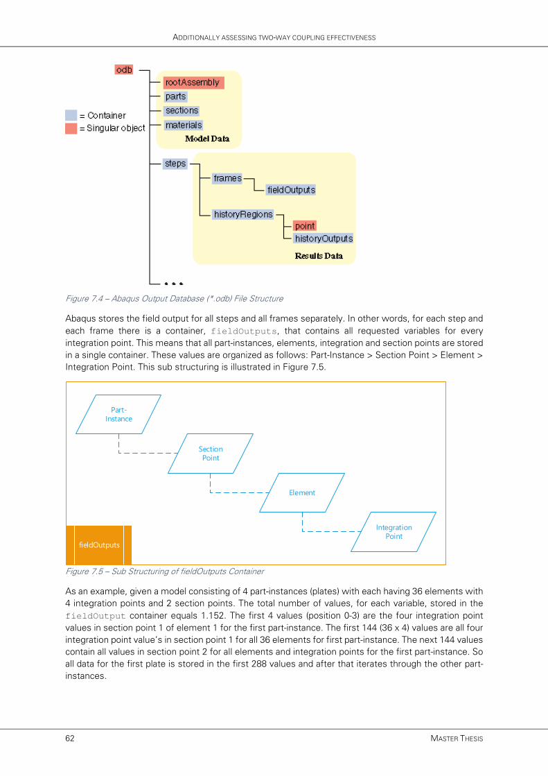
ADDITIONALLY ASSESSING TWO-WAY COUPLING EFFECTIVENESS
62 MASTER THESIS
Figure 7.4 – Abaqus Output Database (*.odb) File Structure
Abaqus stores the field output for all steps and all frames separately. In other words, for each step and
each frame there is a container, fieldOutputs, that contains all requested variables for every
integration point. This means that all part-instances, elements, integration and section points are stored
in a single container. These values are organized as follows: Part-Instance > Section Point > Element >
Integration Point. This sub structuring is illustrated in Figure 7.5.
Part-Instance
Section Point
Element
Integration Point
fieldOutputs
Figure 7.5 – Sub Structuring of fieldOutputs Container
As an example, given a model consisting of 4 part-instances (plates) with each having 36 elements with
4 integration points and 2 section points. The total number of values, for each variable, stored in the
fieldOutput container equals 1.152. The first 4 values (position 0-3) are the four integration point
values in section point 1 of element 1 for the first part-instance. The first 144 (36 x 4) values are all four
integration point value’s in section point 1 for all 36 elements for first part-instance. The next 144 values
contain all values in section point 2 for all elements and integration points for the first part-instance. So
all data for the first plate is stored in the first 288 values and after that iterates through the other part-
instances.

FDS-2-ABAQUS: C++ MANAGED AUTOMATED PYTHON SCRIPTED CFD-FEM COUPLING
J.A. FEENSTRA 63
REQUESTING OUTPUT VALUES
Specific values in the output database can be requested using python code. Assuming the same model
from the previously discussed example (4 part-instances, 2 section points, 36 elements, 4 integration
points). First we need to open our example.odb file:
… from odbAccess import openOdb odb = openOdb('path/example.odb')
…
It is important to note that in python a list starts with 0 and finish with N-1 where N is the number of
elements in the list. The von Mises stress at position 478 (actually the 479th value) can be obtained as
follows (the print command is used to actually output the value):
… stress = odb.steps['stepname'].frames[-1].fieldOutputs['S'] print stress.values[478].mises
…
The corresponding part-instance (name), section point, element number and integration point for
position 478 can be obtained respectively as follows:
… print stress.values[478].instance.name
print stress.values[478].sectionPoint.number
print stress.values[478].elementLabel
print stress.values[478].integrationPoint …
It is quite tedious to iterate through the whole fieldOutput container when only interested in the
values for specific locations. To obtain values for a specific location, i.e. a plate-instance, element(set),
or node(set), the getSubset command is used. As an example the following lines limit the return
values from the fieldOutput container to only include the stresses for the first element of
Plate-1.
…
### Select First Instance ###
instanceName = odb.rootAssembly.instances.keys()[0]
selectInstance = odb.rootAssembly.instances[instanceName]
### Select First Element ###
selectElement = selectInstance.elements[0]
### Subset Containing Stress Data For Element-1 of Plate-1 ###
elementStressField = stressField.getSubset(
region = selectElement,
position = INTEGRATION_POINT,
elementType = 'S8R'
) …
The brief discussion above covers the basic python commands to explore an *.odb output database.
For extensive information on using the scripting interface to access and explore an output database is
referred to the Abaqus Scripting User’s Guide chapter 9 and the Abaqus Scripting Reference Guide
chapter 34 [33].
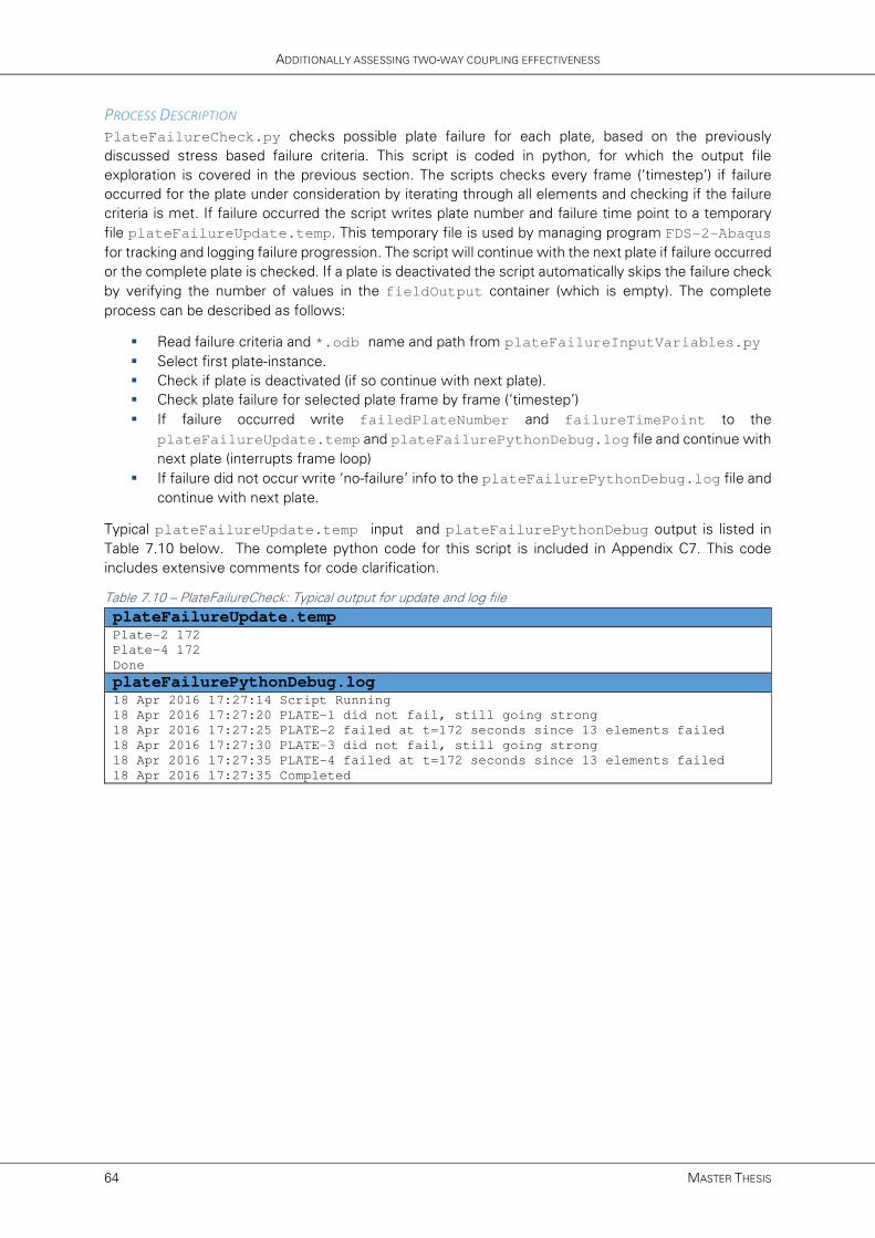
ADDITIONALLY ASSESSING TWO-WAY COUPLING EFFECTIVENESS
64 MASTER THESIS
PROCESS DESCRIPTION
PlateFailureCheck.py checks possible plate failure for each plate, based on the previously
discussed stress based failure criteria. This script is coded in python, for which the output file
exploration is covered in the previous section. The scripts checks every frame (‘timestep’) if failure
occurred for the plate under consideration by iterating through all elements and checking if the failure
criteria is met. If failure occurred the script writes plate number and failure time point to a temporary
file plateFailureUpdate.temp. This temporary file is used by managing program FDS-2-Abaqus
for tracking and logging failure progression. The script will continue with the next plate if failure occurred
or the complete plate is checked. If a plate is deactivated the script automatically skips the failure check
by verifying the number of values in the fieldOutput container (which is empty). The complete
process can be described as follows:
� Read failure criteria and *.odb name and path from plateFailureInputVariables.py
� Select first plate-instance.
� Check if plate is deactivated (if so continue with next plate).
� Check plate failure for selected plate frame by frame (‘timestep’)
� If failure occurred write failedPlateNumber and failureTimePoint to the
plateFailureUpdate.temp and plateFailurePythonDebug.log file and continue with
next plate (interrupts frame loop)
� If failure did not occur write ‘no-failure’ info to the plateFailurePythonDebug.log file and
continue with next plate.
Typical plateFailureUpdate.temp input and plateFailurePythonDebug output is listed in
Table 7.10 below. The complete python code for this script is included in Appendix C7. This code
includes extensive comments for code clarification.
Table 7.10 – PlateFailureCheck: Typical output for update and log file
plateFailureUpdate.temp Plate-2 172
Plate-4 172
Done plateFailurePythonDebug.log 18 Apr 2016 17:27:14 Script Running
18 Apr 2016 17:27:20 PLATE-1 did not fail, still going strong
18 Apr 2016 17:27:25 PLATE-2 failed at t=172 seconds since 13 elements failed
18 Apr 2016 17:27:30 PLATE-3 did not fail, still going strong
18 Apr 2016 17:27:35 PLATE-4 failed at t=172 seconds since 13 elements failed
18 Apr 2016 17:27:35 Completed
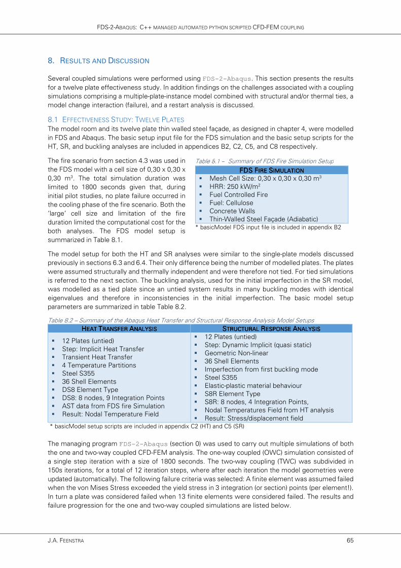
FDS-2-ABAQUS: C++ MANAGED AUTOMATED PYTHON SCRIPTED CFD-FEM COUPLING
J.A. FEENSTRA 65
8. RESULTS AND DISCUSSION
Several coupled simulations were performed using FDS-2-Abaqus. This section presents the results
for a twelve plate effectiveness study. In addition findings on the challenges associated with a coupling
simulations comprising a multiple-plate-instance model combined with structural and/or thermal ties, a
model change interaction (failure), and a restart analysis is discussed.
8.1 EFFECTIVENESS STUDY: TWELVE PLATES
The model room and its twelve plate thin walled steel façade, as designed in chapter 4, were modelled
in FDS and Abaqus. The basic setup input file for the FDS simulation and the basic setup scripts for the
HT, SR, and buckling analyses are included in appendices B2, C2, C5, and C8 respectively.
The fire scenario from section 4.3 was used in
the FDS model with a cell size of 0,30 x 0,30 x
0,30 m3. The total simulation duration was
limited to 1800 seconds given that, during
initial pilot studies, no plate failure occurred in
the cooling phase of the fire scenario. Both the
‘large’ cell size and limitation of the fire
duration limited the computational cost for the
both analyses. The FDS model setup is
summarized in Table 8.1.
The model setup for both the HT and SR analyses were similar to the single-plate models discussed
previously in sections 6.3 and 6.4. Their only difference being the number of modelled plates. The plates
were assumed structurally and thermally independent and were therefore not tied. For tied simulations
is referred to the next section. The buckling analysis, used for the initial imperfection in the SR model,
was modelled as a tied plate since an untied system results in many buckling modes with identical
eigenvalues and therefore in inconsistencies in the initial imperfection. The basic model setup
parameters are summarized in table Table 8.2.
Table 8.2 – Summary of the Abaqus Heat Transfer and Structural Response Analysis Model Setups
HHHHEAT EAT EAT EAT TTTTRANSFER RANSFER RANSFER RANSFER AAAANALYSISNALYSISNALYSISNALYSIS SSSSTRUTRUTRUTRUCTURAL CTURAL CTURAL CTURAL RRRRESPONSEESPONSEESPONSEESPONSE AAAANALYSISNALYSISNALYSISNALYSIS
� 12 Plates (untied)
� Step: Implicit Heat Transfer
� Transient Heat Transfer
� 4 Temperature Partitions
� Steel S355
� 36 Shell Elements
� DS8 Element Type
� DS8: 8 nodes, 9 Integration Points
� AST data from FDS fire Simulation
� Result: Nodal Temperature Field
� 12 Plates (untied)
� Step: Dynamic Implicit (quasi static)
� Geometric Non-linear
� 36 Shell Elements
� Imperfection from first buckling mode
� Steel S355
� Elastic-plastic material behaviour
� S8R Element Type
� S8R: 8 nodes, 4 Integration Points,
� Nodal Temperatures Field from HT analysis
� Result: Stress/displacement field * basicModel setup scripts are included in appendix C2 (HT) and C5 (SR)
The managing program FDS-2-Abaqus (section 0) was used to carry out multiple simulations of both
the one and two-way coupled CFD-FEM analysis. The one-way coupled (OWC) simulation consisted of
a single step iteration with a size of 1800 seconds. The two-way coupling (TWC) was subdivided in
150s iterations, for a total of 12 iteration steps, where after each iteration the model geometries were
updated (automatically). The following failure criteria was selected: A finite element was assumed failed
when the von Mises Stress exceeded the yield stress in 3 integration (or section) points (per element!).
In turn a plate was considered failed when 13 finite elements were considered failed. The results and
failure progression for the one and two-way coupled simulations are listed below.
Table 8.1 – Summary of FDS Fire Simulation Setup
FDSFDSFDSFDS FFFFIRE IRE IRE IRE SSSSIMULATIONIMULATIONIMULATIONIMULATION
� Mesh Cell Size: 0,30 x 0,30 x 0,30 m3
� HRR: 250 kW/m2
� Fuel Controlled Fire
� Fuel: Cellulose
� Concrete Walls
� Thin-Walled Steel Façade (Adiabatic)
* basicModel FDS input file is included in appendix B2

ADDITIONALLY ASSESSING TWO-WAY COUPLING EFFECTIVENESS
66 MASTER THESIS
ONE WAY COUPLED TWO WAY COUPLED duration
iteration size
iterations
1800 s
1800 s
1
duration
iteration size
iterations
1800 s
150 s
12
RESULTS COUPLING ANALYSIS Table 8.3 – Failure time [s] of plates for the one-way coupled analysis.
PLATE
[#]
ONE WAY COUPLED SIMULATION [#]
1 2 3 4 5
01 680 830 955 714 655
02 765 715 745 714 680
03 610 620 590 639 605
04 405 360 450 664 655
05 0 0 0 0 0
06 675 595 615 0 0
07 0 0 0 0 0
08 0 0 0 0 0
09 0 0 0 0 0
10 0 0 0 0 0
11 1345 1525 1750 1789 1305
12 640 660 635 614 605
* failure time in seconds (if 0 s, plate did not fail)
Table 8.4 - Failure time [s] of plates for the two-way coupled analysis.
PLATE
[#]
TWO WAY COUPLED SIMULATION [#]
1 2 3 4 5
01 0 0 0 0 0
02 0 0 0 0 0
03 0 0 0 0 0
04 330 310 440 402 402
05 0 0 0 0 0
06 0 0 0 0 0
07 0 0 0 0 0
08 0 0 0 0 0
09 0 0 0 0 0
10 0 0 0 0 0
11 0 0 0 0 0
12 1690 1690 1690 1752 0
* failure time in seconds (if 0 s, plate did not fail)
Figure 8.1 – Number of failed plates over time for the one-way coupled analysis
Figure 8.2 – Number of failed plates over time for the two-way coupled analysis
FAILURE PROGRESSION [PLATE #]:
4 4 4 4 –––– 3 3 3 3 –––– (6) (6) (6) (6) –––– 12 12 12 12 –––– 2 2 2 2 –––– 1 1 1 1 –––– 11111111
4 4 4 4 –––– (12)(12)(12)(12)
* continues on next page
0
1
2
3
4
5
6
7
8
0 300 600 900 1200 1500 1800
nu
mb
erO
fFa
ile
dP
late
s [#
]
Time [s]
OWC1
OWC2
OWC3
OWC4
OWC5
0
1
2
3
4
5
6
7
8
0 300 600 900 1200 1500 1800
nu
mb
erO
fFa
ile
dP
late
s [#
]
Time [s]
TWC1
TWC2
TWC3
TWC4
TWC5
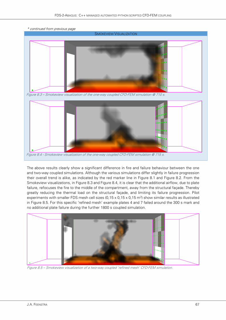
FDS-2-ABAQUS: C++ MANAGED AUTOMATED PYTHON SCRIPTED CFD-FEM COUPLING
J.A. FEENSTRA 67
* continued from previous page
SMOKEVIEW VISUALIZATION
Figure 8.3 – Smokeview visualization of the one-way coupled CFD-FEM simulation @ 710 s.
Figure 8.4 - Smokeview visualization of the one-way coupled CFD-FEM simulation @ 715 s.
The above results clearly show a significant difference in fire and failure behaviour between the one
and two-way coupled simulations. Although the various simulations differ slightly in failure progression
their overall trend is alike, as indicated by the red marker line in Figure 8.1 and Figure 8.2. From the
Smokeview visualizations, in Figure 8.3 and Figure 8.4, it is clear that the additional airflow, due to plate
failure, refocuses the fire to the middle of the compartment, away from the structural façade. Thereby
greatly reducing the thermal load on the structural façade, and limiting its failure progression. Pilot
experiments with smaller FDS mesh cell sizes (0,15 x 0,15 x 0,15 m3) show similar results as illustrated
in Figure 8.5. For this specific ‘refined mesh’ example plates 4 and 7 failed around the 300 s mark and
no additional plate failure during the further 1800 s coupled simulation.
Figure 8.5 – Smokeview visualization of a two-way coupled ‘refined mesh’ CFD-FEM simulation.

ADDITIONALLY ASSESSING TWO-WAY COUPLING EFFECTIVENESS
68 MASTER THESIS
In another pilot the bottom row of the plates was
excluded from the simulation. The idea was, based on the
failure progression of the twelve plate simulations, a top
row panel would fail first given the bottom row failure in
the twelve plate studies were soon followed by top row
failures. These top row failures would then induce a
different airflow resulting in a non-centrally located fire
and thereby a different failure progression. Similar input
parameters to those described in Table 8.1 and Table 8.2
for the FDS, HT, and SR models were used, their only
difference being the use of eight plates compared to the
twelve previously. The first panels failed around the
650 – 800 second mark for both the OWC and TWC
analysis as listed in Table 8.5. No additional failure was
recorded for the two-way coupling possibly due to energy
release to the outside. The Smokeview visualization of
the TWC analysis is included in Figure 8.6.
Figure 8.6 – Smokeview visualization of the two-way coupled CFD-FEM simulation @ 865 s.
An additional remark is that slightly varying the input variables influence the failure time and progression.
Pilot experiments showed that changing the initial imperfections, interval of fieldOutput requests,
and varying the coupling iteration size all affected the failure progression. A detailed parameter study,
possibly verified using real life fire simulations, could help in both mapping and understanding these
influences. Nevertheless the overall failure progression remained relatively identical.
The main drawback of above experiment is that a fuel controlled fire is assumed. Compartment fires in
real life situations typically are, after flashover, ventilation controlled. Plate failure in a ventilation
controlled fire would result in an additional oxygen source causing backdraft and an overall increase in
HRR. Possibly accelerating the failure progression of a two-way coupled simulation compared to a one-
way coupled one. Initial pilot experiments were conducted to include a ventilation controlled fire model
in the simulations. These pilots showed that a fire cannot be defined as a prescriptive HRR curve, as
discussed in section 5.2, to model a ventilation controlled fire. A more complex pyrolysis model needs
to be developed to model a ventilation controlled fire in the simulation. For additional reading on defining
a more complex pyrolysis model is referred to the FDS user’s Guide section 8.5 [27].
All in all it is still too early to give an all conclusive answer on its effectiveness but is clear that the
influence is of significant magnitude for further analysis. Especially considering the many possible
improvements to the various models, scripts and simulations. For additional reading on possible
improvements and recommendations for future research is referred to section 9.2.
Table 8.5 – Failure time [s] and progression for 8-plate OWC and TWC Analysis.
PLATE [#] OWC TWC
01 1020 0
02 800 682
03 0 0
04 0 0
05 0 0
06 0 0
07 915 0
08 710 682
FAILURE
PROGRESSIO8 – 2 – 7 – 1 8 – 2
* failure time in seconds
(if 0 s, plate did not fail)

FDS-2-ABAQUS: C++ MANAGED AUTOMATED PYTHON SCRIPTED CFD-FEM COUPLING
J.A. FEENSTRA 69
8.2 TIED MULTI PLATE MODELS
In the effectiveness study the multiple plates were assumed
structurally and thermally independent, in other words they
were untied. Tying the plates influences the temperature and
stress field of the model and subsequently its failure
progression. However coupling simulations comprising a
multiple-plate-instance model combined with structural and/or
thermal ties, a model change interaction (failure), and a restart
analysis, proofed difficult. This section will explore the findings
of and discuss possible solutions to these challenges.
Various pilot studies were carried out to study the two-way-
coupling of a CFD fire simulation with a structurally and
thermally tied multiple plate Heat Transfer and Structural
response analysis. Tying plates in a one way coupled CFD-FEM
analysis is pretty straight forward as illustrated in the resulting
stress field of a one-way coupled four plate model with thermal
and structural TIE constraints as shown in Figure 8.7. However
it gets challenging when a model change and/or a restart
analysis is introduced. When tying together nodes, a constraint
is defined that describes the displacement (or temperature) of
nodes from plate-2 as a linear combination of the
displacement of nodes from plate-1. Where the so called
slave nodes depend on the master nodes. Therefore when
defining tie constraints a master and a slave node set or surface
is defined (see section 6.5) where the slaves depend on the
masters. Consequently when introducing a model change in an
analysis either a master or a slave plate is deactivated. In
addition one could choose to also deactivate the TIEs between
these plates. The last parameter is that the analysis is either an
initial step or a restart step. Two plate pilot experiments were
set up varying these parameters. A sketch of this pilot model
is included in Figure 8.8 and the results are summarized in
Table 8.6 for the HT analysis and Table 8.7 for the SR analysis.
These results will be discussed in more detail in the following
subsections.
HEAT TRANSFER TIE CONSTRAINTS
In the HT analysis the plates were tied using a master and slave
surface definition. Deactivating the slave surface did not
complicate the initial nor the restart analysis. This is pretty
straight forward since the slave nodes depend on the master nodes in the TIE constraints and can be
deactivated without deactivating variables in the constraint equations. However when deactivating a
master surface the analysis aborts due to the occurrence of zero pivots. A zero pivot occurs when a
term in the load vector corresponds to a dof that has no terms in the stiffness matrix. Basically the
response of the slave nodes depends on master nodes that are no longer active, and therefore aborts.
For the initial analysis (non restart) a possible work-around is to deactivate both the master surface and
suppress the TIE constraints associated with this surface. Thereby omitting the dependencies and
hence the analysis runs successfully. However this does not work for a restart analysis possibly due to
the ‘history’ dependency of these nodes. A possible solution to this approach is to define a new ‘initial’
heat transfer analysis for every iteration in the two way coupling and importing the temperatures from
the previous iteration as boundary condition. Basically just getting rid of the restart analysis. The main
challenge here lies in redeveloping the upGeomHT program to supress TIE constraints when a
corresponding master surface is deactivated. Another approach is to model the wall as an assembly of
Figure 8.7 – Typical Stress Field for one-way coupled four plate model with structural and thermal TIE constraints.
Figure 8.8 – Sketch: Two plate pilot model

ADDITIONALLY ASSESSING TWO-WAY COUPLING EFFECTIVENESS
70 MASTER THESIS
a single façade part containing multiple plate-area’s that can be deactivated. Effectively removing the
ties and therefore the challenges associated with the ties. Although this would work for this specific
simplified ‘wall-as-plate’ approach it will not work for more detailed models, for instance a façade wall
assembled from several column-, strut- and plate instances as previous shown in Figure 6.2. A third
possible solution is to effectively remove the plate by increasing its conductance, more specifically to
gradually adjust the material properties to effectively remove the plate. In absolute terms the plate is
still there but the due to its adjusted material properties it is effectively removed. The main advantage
of this approach is that no plate deactivations nor the suppression of TIE constraint need to be
introduced in the model.
Table 8.6 – Results and possible errors for initial and restart HT analysis on a multiple plate model varying ties and model change interactions.
INITIAL ANALYSIS (HT)
TIE MASTER SLAVE RESULT ERROR
active active deactivated Completed -
active deactivated active Aborted Zero Pivot, Nodal temp below 0 K
supressed deactivated active Completed -
RESTART ANALYSIS (HT)
active active deactivated Completed -
active deactivated active Aborted Solver Problem Zero Pivot
supressed deactivated active Aborted Solver Problem Zero Pivot
In summary: Due to the dependency of slave nodes on master nodes deactivating these master nodes
will cause a singularity in the constraint equations, thereby complicating and possibly crashing the
analysis. Possible solutions are:
� Supress TIE constraints when deactivating master surface and omit restart analyses.
� Model façade as single part, effectively removing TIE constraints.
� Effectively remove plate by increasing its conductance.
STRUCTURAL RESPONSE TIE CONSTRAINTS
In the SR analysis the plates were tied using a master and slave
edge definition. As with the HT analysis deactivating the slave
did not influence the initial nor the restart analysis. In addition,
for this two plate pilot, both the initial and restart analysis ran
successfully when deactivating the master. The difference in
job completion between the HT and SR analysis is due to the
TIE constraint definition based on edges (SR) compared to the
constraints based on surfaces (HT) when deactivating a plate-
area the edge sets are still valid while surface sets are
deactivated. Supressing the TIE constraints associated with a
deactivated master plate resulted in an unstable simulation.
This is pretty straight forward given boundary conditions are
prescribed for the master nodes only to avoid over constraining
the slave nodes. When a TIE is supresses the slave plate is cut
loose allowing for unconstrained rotation (rigid body) as
illustrated in Figure 8.9. So either the TIE constraints should
remain active or initially suppressed boundary conditions on the
slave nodes should be reactivated.
Figure 8.9 – rigid body rotation when deactivating master and supressing TIE constraint (master shown for clarity)

FDS-2-ABAQUS: C++ MANAGED AUTOMATED PYTHON SCRIPTED CFD-FEM COUPLING
J.A. FEENSTRA 71
Table 8.7 - Results and possible errors for initial and restart SR analysis on a multiple plate model varying ties and model change interactions.
INITIAL ANALYSIS (SR)
TIE MASTER SLAVE RESULT ERROR
active active deactivated Completed -
active deactivated active Completed -
supressed deactivated active Aborted Unstable, not enough displacement BC
RESTART ANALYSIS (SR)
active active deactivated Completed -
active deactivated active Completed (does not work for 4-plate system)
supressed deactivated active Aborted Unstable, not enough displacement BC
At first sight these SR analyses seemed less challenging but
the real challenge occurred while expanding the two plate pilot
to a four plate pilot as illustrated in Figure 8.10. For the initial
(non restart) simulation both the master and slave plates could
be deactivated without causing convergence errors. But when
deactivating a master edge in the four plate pilot the ‘edge
curling’ and ultimately convergence error illustrated in Figure
8.11 occurred. The reason this error did not occur during the
previous two plate pilot is because of the hinged boundary
conditions on the top and bottom of the plates. The removal of
a plate causes a sudden stress and stiffness change which
proofed too challenging for the solver. A possible solution is to
introduce some sort of ‘relaxation’ step to reinitialize the
changed model. Another approach is to effectively remove the
plate by gradually lowering its stiffness (factor 0.001), similar to
the HT approach discussed previously.
Figure 8.11 – Edge ‘curling’ discontinuity due to sudden stress and stiffness change.
In summary: The model change interaction causes a sudden stress and stiffness change which proofed
too challenging for a restart analysis. Possible solutions are:
� Introduce a ‘relaxation’ step as transition between complete and partly failed model.
� Effectively remove plate by lowering its stiffness.
Figure 8.10 - Sketch: Four plate pilot model

FDS-2-ABAQUS: C++ MANAGED AUTOMATED PYTHON SCRIPTED CFD-FEM COUPLING
J.A. FEENSTRA 73
9. CONCLUSIONS AND RECOMMENDATIONS
In this chapter the thesis is finalized by drawing conclusions and a separate section on
recommendations for future research containing an extensive discussion on possible improvements to
the two-way coupling approach and FDS-2-Abaqus.
9.1 CONCLUSIONS
This thesis set out to explore the feasibility of two-way coupled CFD fire simulations to FE heat transfer
and structural response analysis. Basically it aimed to answer the questions ‘Can we do it?’ and ‘Should
we do it?’ More specifically it aimed to compare the effectiveness of a one-way coupled to a two-way
coupled analysis by first identifying the various analysis steps, both how to perform and implement
them in a coupled analysis. Secondly by studying the coupling steps and analyse the typical data
exchange between the various analysis steps. And finally provide necessary tools to facilitate this
coupling using programs and scripts.
Extensive discussions and explanations on performing and implementing the various analysis and
coupling steps were included in their respective chapters (4 - 7). In addition the programs and scripts
developed to facilitate a two-way coupling were discussed and summarized in chapter 7. So over the
course of these chapters the ‘Can we do it?’ was answered implicitly by both explaining a possible
approach to, and performing a two-way coupling.
The more interesting question, however, is should we perform such types of analysis. Initial studies
using the FDS-2-Abaqus program developed throughout this thesis illustrated a significant difference
in the failure progression of a façade wall between a one-way and two-way coupled analysis. This
difference was governed by the change in fire propagation due to geometric updates in the fire, heat
transfer, and structural response models. However it is still too early to give an all conclusive answer
on its effectiveness mainly due to the lack of validation and the simplified approach to reality. Still it is
clear that the influence is of significant magnitude for further analysis. Especially considering the many
possible improvements to the various models, scripts and simulations.
Although limited in its current state FDS-2-Abaqus and this thesis can be seen as the preliminary
framework for the use of two-way coupling in the field of structural fire and safety engineering. More
specifically it could contribute to a better understanding of both structural response to fire and the
response of the fire propagation to these structural changes. Therefore it could proof a powerful tool
for research on fire propagation and structural response. For instance allowing extensive parameter
studies on specific scenarios which would be virtually impossible, or economically impracticable, to
study with real life in-situ experiments.
The biggest limitations of this research are found in the initial assumptions, the lack of validation, and
the specific applications to FDS and Abaqus. Although the overall concept and approach should be
applicable to other CFD and FE codes. In addition FDS-2-Abaqus and its subprograms are, in its current
state, limited to studying structural systems consisting of a limited number of plate-instances. For a
detailed discussion on possible improvements and future research is referred to the next section.
In a way, the program FDS-2-Abaqus is itself the conclusion. FDS-2-Abaqus proofs the concept of
two-way coupling, while illustrating the difference in fire and failure propagation of a two-way coupling
compared to a one-way coupled analysis. In addition FDS-2-Abaqus provides the opportunity to
perform various two-way coupled fire-to-thermomechanical studies.

ADDITIONALLY ASSESSING TWO-WAY COUPLING EFFECTIVENESS
74 MASTER THESIS
9.2 RECOMMENDATIONS FOR FUTURE RESEARCH
During the initial phase of the research various assumptions were made and simplifications introduced,
which, in retrospect proofed suboptimal. For instance, the combination of model change interactions
with a restart analysis as extensively discussed in section 8.2 or the simplified approach to fire as a fuel
controlled fire compared to a more realistic ventilation controlled compartment fire. Nevertheless, as
previously mentioned, this thesis can be seen as the framework for performing two way coupled fire
to thermomechanical analysis and by tackling various challenges become an even more powerful
research tool. Various improvements and recommendations are discussed in this section subdivided
into the separate analysis and coupling steps. In addition the consequences of the improvements on
FDS-2-Abaqus and its subprograms are discussed.
FDS MODEL AND FIRE SIMULATION
The values for fire load and heat release rate in the FDS simulation were based on literature and
implemented as an equally spread fire load with a constant HRR till decay phase. The total floor area
was ablaze simulating a post flashover fire. A real life fire is far more random and strongly depends on
the occupancy class, interior, and size of the openings. Where a post flashover fire is fuel controlled in
case of large openings and ventilation (oxygen) controlled in case of small opening in the boundaries. A
more realistic fire model could include a fully modelled interior, using a ventilation controlled fire and a
fire scenario from initial to cooling phase. Modelling a ventilation controlled fire would greatly influence
the failure progression in a two-way coupled analysis since partial collapse could result in an additional
oxygen supply causing backdraft and an overall increase in HRR. Which in turn increases the thermal
load on the structure, possibly causing failure, and so on. The redevelopment of the FDS simulation
comprising a more realistic fire model and fire scenario would contribute to a more conclusive answer
on the feasibility of two-way coupling. A possible implementation of a more advanced model is found
in the definition of a complex pyrolysis model as described in the FDS user’s Guide section 8.5 [27].
The main advantage for this improvement is that it can be studied separately. Meaning no additional
changes are necessary to the other models, programs, and scripts. Although the structural model would
be limited to one consisting of multiple plates utilizing a failure criteria based on exceeding the Von
Mises stress.
EFFECTIVELY REMOVE PLATES
The challenge in combining TIE constraints with model change interactions and a restart analysis has
been discussed extensively in section 8.2. The absolute removal of plates, using model change
interactions, proofed suboptimal mainly due to the reliance of slave nodes on master nodes and the
sudden changes in the stress field when removing plates. A possible solution is to redevelop the heat
transfer model to effectively remove plates by gradually increasing its thermal conductance. Similarly
the structural response model could be redeveloped to effectively remove plates by gradually lowering
its stiffness. Using this approach both challenges could be tackled. Extensive pilot experiments should
be set up to test this hypothesis.
Redevelopment of the HT and SR models to effectively remove failed plates influences both the
basicModel setups and the additional code appended by the upGeom programs. Consequently the
upGeomHT and upGeomSR programs need to be redeveloped to include lines to gradually increase or
lower the material properties of failed plates. More specifically the append_update_geometry
function in both these programs which appends the plate deactivation code should be redesigned. The
C++ source code for the upGeomHT and upGeomSR programs are included in appendix D4 and D5
respectively.

FDS-2-ABAQUS: C++ MANAGED AUTOMATED PYTHON SCRIPTED CFD-FEM COUPLING
J.A. FEENSTRA 75
In addition a few lines in PlateFailureCheck.py need to be redeveloped. When deactivating a plate-
instance in a model the fieldOutput container, for this specific instance, returns empty.
PlateFailureCheck.py currently checks if a container is empty, and if so, skips it since it has already
failed and should not be checked. When effectively removing them this approach will not work. It is
advised to rewrite these lines. A possible solution is to perform this check based on the material
properties of the plate. Additionally the script could be rewritten to use the _plateFailure.log file
managed by FDS-2-Abaqus similar to the upGeom programs.
ABAQUS MODELS AND SIMULATIONS
In the initial stage of this research a model room was developed using a thin walled steel façade. This
thin walled steel façade was simplified to a wall consisting of steel panels supported by a frame. The
frame was modelled as hinged boundary conditions imposed on the top and bottom of the plates. Thin
walled steel façade system consist of many components (struts, beams, fasteners, insulation, and
panels) which perform differently under fire conditions and influence each other. In addition these
components perform on a different scale-level. Accordingly development of multi scale multi
component heat transfer and structural response models could contribute to more realistic failure
progression and subsequently fire propagation. The main drawback of these multi scale multi
component models is that both the FE models and the coupling tools increase in complexity. On the
other hand it allows for more specific failure criteria’s, for instance failure of fasteners, to be included
in the coupled analysis. In the long run these models could be used in advanced two way coupling
studies that could support and expand upon current in situ experiments.
VALIDATION
No detailed verification or validation studies were performed during the development of FDS-2-
Abaqus. Meaning it strongly depends on the validation of the FDS and Abaqus software. The accuracy
of a CFD calculation dependents on the resolution of the underlying numerical grid. Initial verification
can be completed by performing a grid resolution stud. In addition existing fire tests on thin walled steel
structures could be used to validate the model. Although these validation studies should be preceded
by the development of more advanced (and verified) fire, heat transfer and structural models.
FDS-2-ABAQUS
Currently FDS-2-Abaqus and its subprograms are limited to performing a one or two-way coupled
CFD-FEM analysis comprising a structural system consisting of multiple plates and a failure criteria
based on the Von Mises stress. The program could be upgraded to include a greater variety of structural
systems and failure criteria’s. FDS-2-Abaqus is sub structured into multiple programs each with a
distinct task. These subprograms can be altered independently as long as the new or upgraded program
requires and generates the same input and/or output files. A possible improvement to FDS-2-Abaqus
is to improve the data flow between FDS-2-Abaqus and the FDS and Abaqus Simulations. Allowing,
for instance, to interrupt the coupling procedure when an error in the FDS or Abaqus Simulation is
encountered.


FDS-2-ABAQUS: C++ MANAGED AUTOMATED PYTHON SCRIPTED CFD-FEM COUPLING
J.A. FEENSTRA 77
REFERENCES
[1] Nederlands Normalisatie-instituut (NEN), “Eurocode 1: Actions on structures – Part 1-2: General
actions – Actions on structures exposed to fire,” 2012.
[2] K. Prasad and H. R. Baum, “Coupled fire dynamics and thermal response of complex building
structures,” Proc. Combust. Inst., vol. 30, no. 2, pp. 2255–2262, Jan. 2005.
[3] H. R. Baum, “Simulating fire effects on complex building structures,” Mech. Res. Commun., vol. 38, no. 1, pp. 1–11, 2011.
[4] S. Welch, S. Miles, S. Kumar, T. Lemaire, and A. Chan, “FIRESTRUC - Integrating advanced
three-dimensional modelling methodologies for predicting thermo-mechanical behaviour of steel
and composite structures subjected to natural fires,” Fire Saf. Sci., vol. 9, pp. 1315–1326, 2008.
[5] C. Luo, L. Chen, J. Lua, and P. Liu, “Abaqus Fire Interface Simulator Toolkit (AFIST) for Coupled
Fire and Structural Response Prediction,” in Structures, Structural Dynamics, and Materials Conference, 2010, no. April.
[6] U. Wickström, D. Duthinh, and K. McGrattan, “Adiabatic surface temperature for calculating
heat transfer to fire exposed structures,” Interflam, vol. 2, p. 943, 2007.
[7] D. Duthinh, K. McGrattan, and A. Khaskia, “Recent advances in fire–structure analysis,” Fire Saf. J., vol. 43, no. 2, pp. 161–167, Feb. 2008.
[8] D. Banerjee, W. Hess, T. Olano, J. Terrill, and J. Gross, “Visualization of structural behavior under
fire,” National Institute of Standards and Technology, 2009.
[9] J. C. G. Silva, A. Landesmann, and F. L. B. Ribeiro, “Interface model to fire-thermomechanical
performance-based analysis of structures under fire conditions,” in Fire and Evacuation Modeling Technical Conference (FEMTC) 2014, 2014.
[10] J. C. Silva, “FDS2FTMI - An automated code to one-way coupling between FDS and FEM using
FTMI,” 2016. .
[11] C. Zhang, J. G. Silva, C. Weinschenk, D. Kamikawa, and Y. Hasemi, “Simulation Methodology
for Coupled Fire-Structure Analysis: Modeling Localized Fire Tests on a Steel Column,” Fire Technol., 2015.
[12] D. K. Banerjee, “Software Independent Data Mapping Tool for Structural Fire Analysis.”
[13] L. Stanbrough, Encyclopedia of Natural Hazards, 1st ed. Dordrecht: Springer Netherlands, 2013.
[14] S. Svensson, Fire Ventilation, vol. 46, no. 0. NRS Tryckeri, Huskvarna, 2005.
[15] L.-G. Bengtsson, Enclosure fi res Enclosure fi res. NRS Tryckeri, Huskvarna, 2001.
ADDITIONALLY ASSESSING TWO-WAY COUPLING EFFECTIVENESS
78 MASTER THESIS
[16] M. Fontana, J. Kohler, K. Fischer, and G. De Sanctis, “Fire Load Density,” in SFPE Handbook of Fire Protection Engineering, 5th ed., M. J. Hurley, D. Gottuk, J. R. Hall, K. Harada, E. Kuligowski,
M. Puchovsky, J. Torero, J. M. Watts, and C. Wieczorek, Eds. New York, NY: Springer, 2016,
pp. 1131–1142.
[17] National Research Council Canada; International Code Council (USA); New Zealand. Dept. of
Building and Housing; Australian Building Codes Board, International Fire Engineering Guidelines. Canberra, 2005.
[18] N. Elhami Khorasani, M. Garlock, and P. Gardoni, “Fire load: Survey data, recent standards, and
probabilistic models for office buildings,” Eng. Struct., vol. 58, pp. 152–165, 2013.
[19] European Committee for Standardization, “EN 1991-1-2/NB - National Annex to EN 1991-1-2,
Eurocode 1: Actions on structures – Part 1-2: General actions – Actions on structures exposed
to fire,” 2010.
[20] S. Bryl, “Brandbelastungen im Hochbau,” Scheizerische Bauzetung, vol. 93, no. 17, 1975.
[21] S. Bryl, “Brandbelastung im Stahlbau, Teil III, Brandbelasting in Bürogebäuden, ECCS-III-74-2-
D,” in European Convention for Constructional Steelwork, 1974.
[22] E. Zalok, “Validation of Methodologies to Determine Fire Load For Use in Structural Fire
Protection,” 2011.
[23] Association de établissements cantonaux d’assurance incendie (AEAI), “Note Explicaivive de
Protection Incendie - Evaluation en vue de la détermination de la grandeur des compartiments
coupe-feu (115-03f),” 2003.
[24] National Fire Protection Association (NFPA), “NFPA 557 standard for determination of fire loads
for use in structural fire protection design.,” 2012.
[25] H. D. Young, R. A. Freedman, and A. Lewis Ford, University Physics, 11th ed. San Fransisco: Addison Wesley, 2004.
[26] L. van Meijel and T. Bouma, “Kantoorgebouwen in Nederland 1945-2015 cultuurhistorische en
typologische quickscan,” pp. 1–20, 2013.
[27] K. McGrattan, R. Mcdermott, S. Hostikka, and J. Floyd, “Fire Dynamics Simulator (Version 6)
User ’ s Guide.” p. 262, 2013.
[28] R. Mcdermott, “Sixth Edition Fire Dynamics Simulator Technical Reference Guide Volume 1 :
Mathematical Model,” vol. 1.
[29] K. McGrattan, S. Hostikka, R. McDermott, J. Floyd, C. Weinschenk, and K. Overholt, “Fire
Dynamics Simulator, Technical Reference Guide, Volume 2: Verification,” vol. 4, 2013.

FDS-2-ABAQUS: C++ MANAGED AUTOMATED PYTHON SCRIPTED CFD-FEM COUPLING
J.A. FEENSTRA 79
[30] K. B. McGrattan, S. Hostikka, J. E. Floyd, and R. McDermott, “Fire Dynamics Simulator,
Technical Reference Guide, Volume 3: Experimental Validation,” vol. 3, no. 1018, 2007.
[31] G. P. Forney, “Smokeview (Version 5) A Tool for Visualizing Fire Dynamics Simulation Data
Volume I : User’s Guide,” vol. I, no. Version 5, p. 162, 2010.
[32] P. Huang, “Interview with Mark Goldstein, CEO of Abaqus,” 2005. .
[33] Dassault Systèmes, “Abaqus 6.14 Documentation Collection.” .
[34] Simulia, “Abaqus 6.14 Documentation.” [Online]. Available: http://50.16.225.63/v6.14/.
[Accessed: 10-Sep-2015].

ADDITIONALLY ASSESSING TWO-WAY COUPLING EFFECTIVENESS
80 MASTER THESIS
GGGGRADUATIONRADUATIONRADUATIONRADUATION TTTTHESISHESISHESISHESIS AAAA----2016.1612016.1612016.1612016.161
FDSFDSFDSFDS----2222----AbaqusAbaqusAbaqusAbaqus
C++C++C++C++ MANAGED AUTOMATED PYMANAGED AUTOMATED PYMANAGED AUTOMATED PYMANAGED AUTOMATED PYTHON SCRIPTED THON SCRIPTED THON SCRIPTED THON SCRIPTED CFDCFDCFDCFD----FEMFEMFEMFEM COUPLINGCOUPLINGCOUPLINGCOUPLING
Additionally assessing twoAdditionally assessing twoAdditionally assessing twoAdditionally assessing two----way coupling effectivenessway coupling effectivenessway coupling effectivenessway coupling effectiveness
J.A.Feenstra
0726615
July 2016
APPENDICES

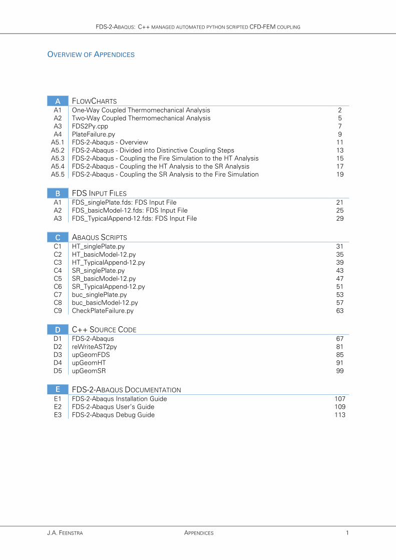
FDS-2-ABAQUS: C++ MANAGED AUTOMATED PYTHON SCRIPTED CFD-FEM COUPLING
J.A. FEENSTRA APPENDICES 1
OVERVIEW OF APPENDICES
AAAA FLOWCHARTS
A1 One-Way Coupled Thermomechanical Analysis 2
A2 Two-Way Coupled Thermomechanical Analysis 5
A3 FDS2Py.cpp 7
A4 PlateFailure.py 9
A5.1 FDS-2-Abaqus - Overview 11
A5.2 FDS-2-Abaqus - Divided into Distinctive Coupling Steps 13
A5.3 FDS-2-Abaqus - Coupling the Fire Simulation to the HT Analysis 15
A5.4 FDS-2-Abaqus - Coupling the HT Analysis to the SR Analysis 17
A5.5 FDS-2-Abaqus - Coupling the SR Analysis to the Fire Simulation 19
BBBB FDS INPUT FILES A1 FDS_singlePlate.fds: FDS Input File 21
A2 FDS_basicModel-12.fds: FDS Input File 25
A3 FDS_TypicalAppend-12.fds: FDS Input File 29
CCCC ABAQUS SCRIPTS C1 HT_singlePlate.py 31
C2 HT_basicModel-12.py 35
C3 HT_TypicalAppend-12.py 39
C4 SR_singlePlate.py 43
C5 SR_basicModel-12.py 47
C6 SR_TypicalAppend-12.py 51
C7 buc_singlePlate.py 53
C8 buc_basicModel-12.py 57
C9 CheckPlateFailure.py 63
DDDD C++ SOURCE CODE D1 FDS-2-Abaqus 67
D2 reWriteAST2py 81
D3 upGeomFDS 85
D4 upGeomHT 91
D5 upGeomSR 99
EEEE FDS-2-ABAQUS DOCUMENTATION E1 FDS-2-Abaqus Installation Guide 107
E2 FDS-2-Abaqus User’s Guide 109
E3 FDS-2-Abaqus Debug Guide 113

ADDITIONALLY ASSESSING TWO-WAY COUPLING EFFECTIVENESS
2 APPENDICES MASTER THESIS

3
APPENDIX A1 – FLOWCHART: ONE-WAY COUPLED THERMOMECHANICAL ANALYSIS

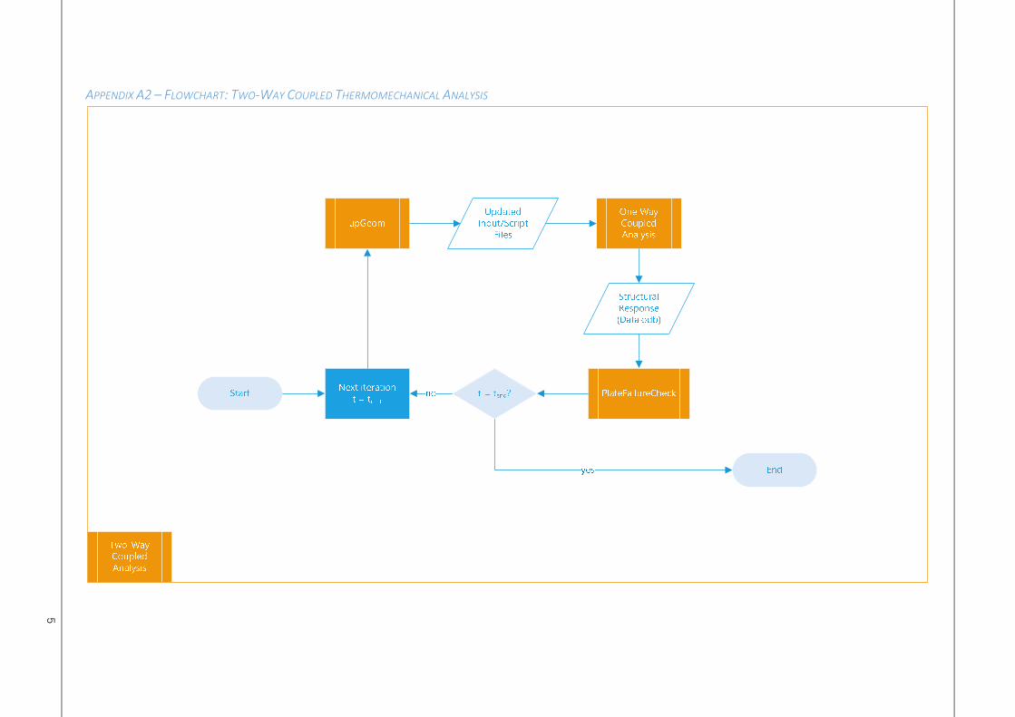
5
APPENDIX A2 – FLOWCHART: TWO-WAY COUPLED THERMOMECHANICAL ANALYSIS

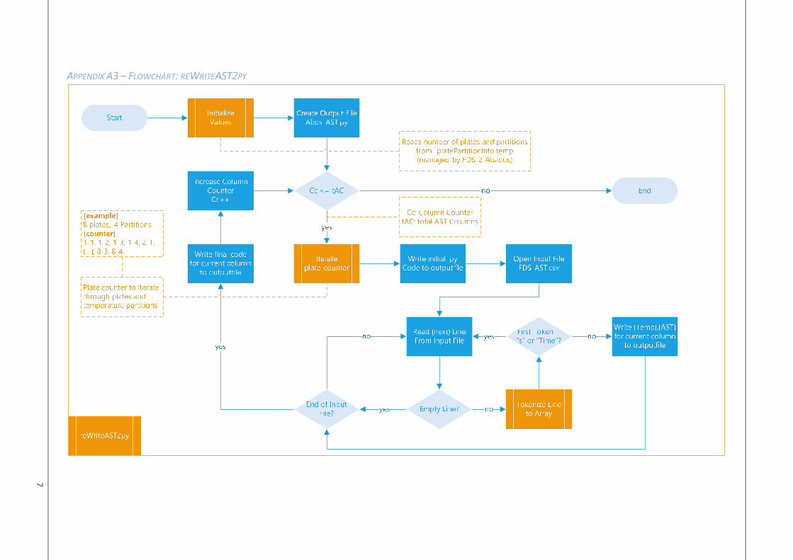
7
APPENDIX A3 – FLOWCHART: REWRITEAST2PY

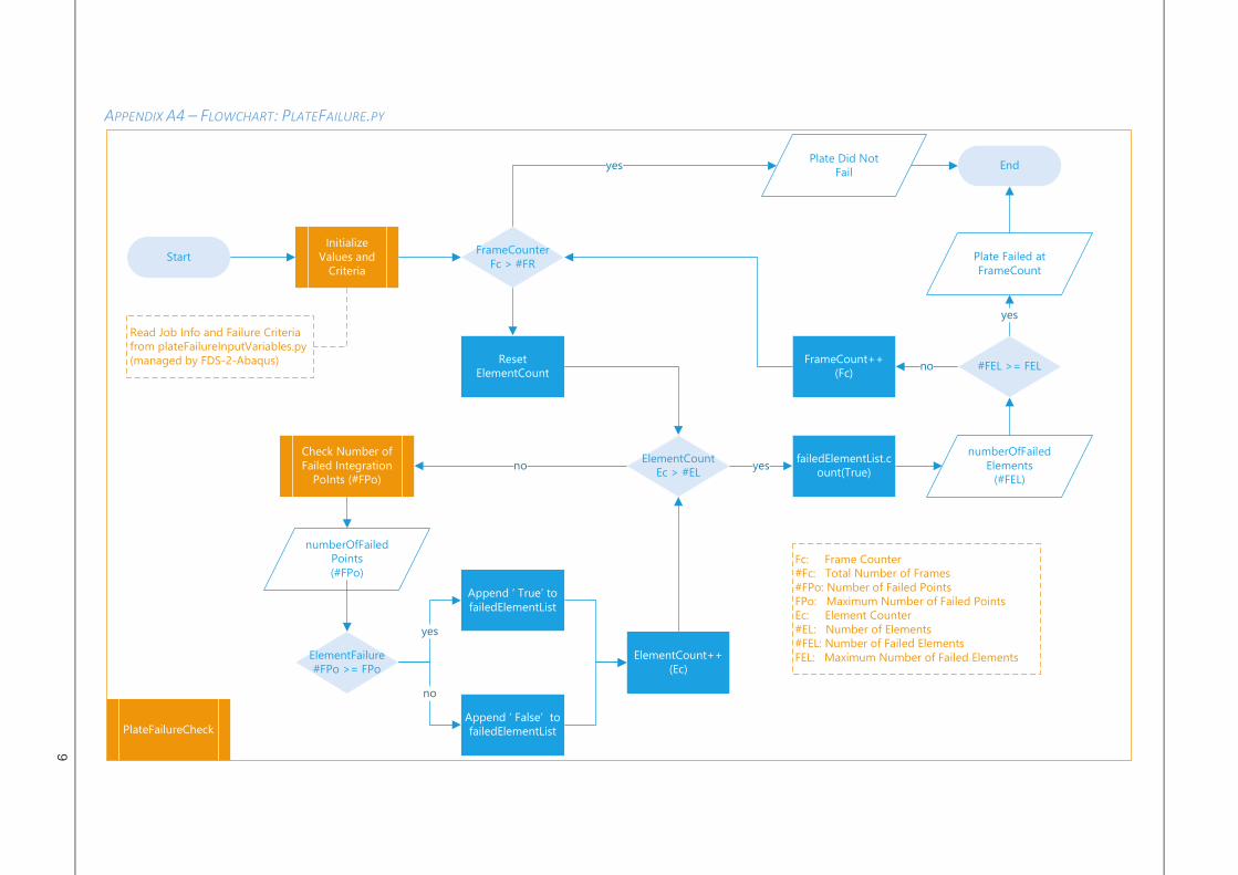
9
APPENDIX A4 – FLOWCHART: PLATEFAILURE.PY
PlateFailureCheck
FrameCounterFc > #FR
Initialize Values and
CriteriaStart
End
#FEL >= FEL
yes
FrameCount++(Fc)
no
Plate Did Not Fail
yes
ElementCountEc > #EL
ElementFailure#FPo >= FPo
Append ‘ True’ to failedElementList
Append ‘ False’ to failedElementList
yes
no
ElementCount++(Ec)
Check Number of Failed Integration
PoInts (#FPo)
numberOfFailedPoints(#FPo)
nofailedElementList.c
ount(True)yes
numberOfFailedElements
(#FEL)
Reset ElementCount
Plate Failed at FrameCount
Read Job Info and Failure Criteria from plateFailureInputVariables.py(managed by FDS-2-Abaqus)
Fc: Frame Counter#Fc: Total Number of Frames#FPo: Number of Failed PointsFPo: Maximum Number of Failed PointsEc: Element Counter#EL: Number of Elements#FEL: Number of Failed ElementsFEL: Maximum Number of Failed Elements


11
APPENDIX A5.1 – FLOWCHART: FDS-2-ABAQUS – OVERVIEW


13
APPENDIX A5.2 – FLOWCHART: FDS-2-ABAQUS – DIVIDED INTO DISTINCTIVE COUPLING STEPS


15
APPENDIX A5.3 – FLOWCHART: FDS-2-ABAQUS – COUPLING OF THE FIRE SIMULATION TO THE HEAT TRANSFER ANALYSIS


17
APPENDIX A5.4 – FLOWCHART: FDS-2-ABAQUS – COUPLING OF THE HEAT TRANSFER ANALYSIS TO THE STRUCTURAL RESPONSE ANALYSIS

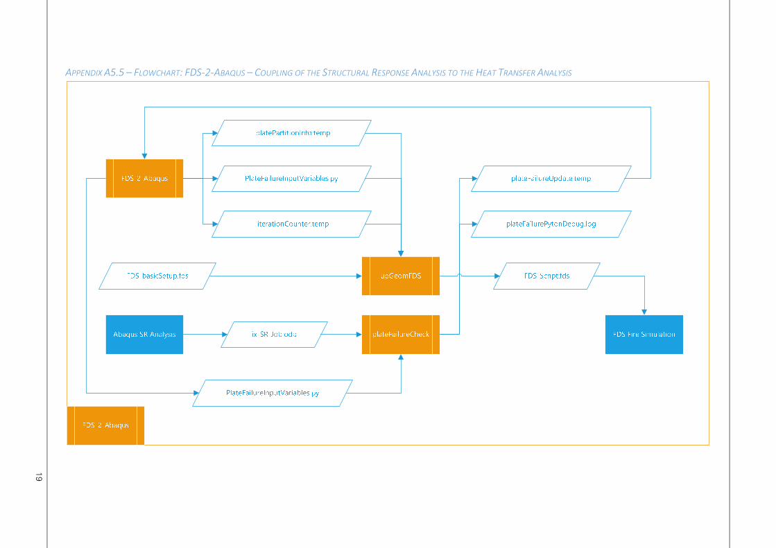
19
APPENDIX A5.5 – FLOWCHART: FDS-2-ABAQUS – COUPLING OF THE STRUCTURAL RESPONSE ANALYSIS TO THE HEAT TRANSFER ANALYSIS


FDS-2-ABAQUS: C++ MANAGED AUTOMATED PYTHON SCRIPTED CFD-FEM COUPLING
J.A. FEENSTRA APPENDICES 21
APPENDIX B1 – FDS_SINGLEPLATE.FDS: FDS INPUT FILE
///////////////////////////////////////////////////////////////////////////
// Name: FDS_singlePlate.fds //
// //
// Description: FDS fire model for a single plate one-way coupled //
// thermo-mechanical CFD-FEM Analysis. //
// //
// //
// Output: FDS_Simulation_devc.csv //
// (Comma separated file containing AST data) //
// //
///////////////////////////////////////////////////////////////////////////
// Version 1.0 by J.A.Feenstra //
// August 2016 [email protected] //
///////////////////////////////////////////////////////////////////////////
//////////////////////////// Begin Input File /////////////////////////////
// Basic Header Info //
&HEAD CHID='FDS_Simulation', TITLE='Basic FDS Model - 12 Plate' /
// Specify Total Simulation Duration //
&TIME T_BEGIN=0, T_END=3650./
// Specify Coordinate system and Discretization //
&MESH IJK=30,12,9, XB=0.0,9.0,0.0,3.6,0.0,2.7 /
// Define Output Request Interval //
&DUMP STATUS_FILES=TRUE, NFRAMES=1460, DT_DEVC=5. /
// Set Default Surface //
&MISC SURF_DEFAULT='CONCRETE_S'
// Define Fuel Type //
&REAC FUEL = 'CELLULOSE'
FORMULA = 'C4H6O3'
// Specify Enthalpy [kJ/mol] for Species //
&SPEC ID = 'CELLULOSE',
FORMULA = 'C4H6O3',
ENTHALPY_OF_FORMATION=-5.13E2 /
// Define Fire Propagation //
&SURF ID='fire',HRRPUA=250.,RAMP_Q='fire',TMP_FRONT=100.,COLOR='RED' /
&RAMP ID='fire',T= 0.,F=0. /
&RAMP ID='fire',T= 10.,F=1. /
&RAMP ID='fire',T=1970.,F=1. /
&RAMP ID='fire',T=3650.,F=0. /
// Define Fire Area //
&VENT XB=1.8,7.2,0.0,3.6,0.0,0.0, SURF_ID='fire' /
// Specify Concrete Material Properties //
// CONDUCTIVITY [W m-1 K-1], DENSITY [kg m-3] //
// SPECIFIC_HEAT [kJ kg-1 K-1], EMISSIVITY //
&MATL ID='CONCRETE_M',
DENSITY=1800.,
CONDUCTIVITY=1.15,
SPECIFIC_HEAT=1.00,
EMISSIVITY=0.80, /
// Define Concrete Surface //
&SURF ID='CONCRETE_S', MATL_ID='CONCRETE_M', THICKNESS=0.3, COLOR='GRAY' /
// Define Adiabatic Surface //
&SURF ID='ADIABATIC', ADIABATIC=.TRUE./
// Specify Corridor Wall (And Door) //
&OBST XB=1.8,1.8,0.0,3.6,0,2.7 /
&HOLE XB=1.6,2.0,0.6,3.0,0.0,2.1 /

ADDITIONALLY ASSESSING TWO-WAY COUPLING EFFECTIVENESS
22 APPENDICES MASTER THESIS
// Define Facade Wall //
// This wall consist of 12 separate obstructions to //
// allow for independent obstruction removal //
// Plate 1 - Column 1, Row 1 //
&OBST XB=7.2,7.2,2.7,3.6,0.0,0.9, SURF_ID='ADIABATIC', COLOR='LIGHT GREY',
DEVC_ID='RemPlate1' /
// Plate 2 - Column 1, Row 2 //
&OBST XB=7.2,7.2,2.7,3.6,0.9,1.8, SURF_ID='ADIABATIC', COLOR='SILVER',
DEVC_ID='RemPlate2' /
// Plate 3 - Column 1, Row 3 //
&OBST XB=7.2,7.2,2.7,3.6,1.8,2.7, SURF_ID='ADIABATIC', COLOR='WARM GREY',
DEVC_ID='RemPlate3' /
// Plate 4 - Column 2, Row 1 //
&OBST XB=7.2,7.2,1.8,2.7,0.0,0.9, SURF_ID='ADIABATIC', COLOR='WARM GREY',
DEVC_ID='RemPlate4' /
// Plate 5 - Column 2, Row 2 //
&OBST XB=7.2,7.2,1.8,2.7,0.9,1.8, SURF_ID='ADIABATIC', COLOR='LIGHT GREY',
DEVC_ID='RemPlate5' /
// Plate 6 - Column 2, Row 3 //
&OBST XB=7.2,7.2,1.8,2.7,1.8,2.7, SURF_ID='ADIABATIC', COLOR='SILVER',
DEVC_ID='RemPlate6' /
// Plate 7 - Column 3, Row 1 //
&OBST XB=7.2,7.2,0.9,1.8,0.0,0.9, SURF_ID='ADIABATIC', COLOR='SILVER',
DEVC_ID='RemPlate7' /
// Plate 8 - Column 3, Row 2 //
&OBST XB=7.2,7.2,0.9,1.8,0.9,1.8, SURF_ID='ADIABATIC', COLOR='ORANGE',
DEVC_ID='RemPlate8' /
// Plate 9 - Column 3, Row 3 //
&OBST XB=7.2,7.2,0.9,1.8,1.8,2.7, SURF_ID='ADIABATIC', COLOR='LIGHT GREY',
DEVC_ID='RemPlate9' /
// Plate 10 - Column 4, Row 1 //
&OBST XB=7.2,7.2,0.0,0.9,0.0,0.9, SURF_ID='ADIABATIC', COLOR='LIGHT GREY',
DEVC_ID='RemPlate10' /
// Plate 11 - Column 4, Row 2 //
&OBST XB=7.2,7.2,0.0,0.9,0.9,1.8, SURF_ID='ADIABATIC', COLOR='SILVER',
DEVC_ID='RemPlate11' /
// Plate 12 - Column 4, Row 3 //
&OBST XB=7.2,7.2,0.0,0.9,1.8,2.7, SURF_ID='ADIABATIC', COLOR='WARM GREY',
DEVC_ID='RemPlate12' /
// Define Vents //
// Removing Obstructions outside Office Space (Front) //
&VENT XB=0.0,1.8,0.0,3.6,0.0,0.0, SURF_ID='OPEN' /
&VENT XB=0.0,1.8,0.0,3.6,2.7,2.7, SURF_ID='OPEN' /
&VENT XB=0.0,1.8,0.0,0.0,0.0,2.7, SURF_ID='OPEN' /
&VENT XB=0.0,1.8,3.6,3.6,0.0,2.7, SURF_ID='OPEN' /
&VENT MB='XMIN', SURF_ID='OPEN' /
// Removing Obstructions outside Office Space (Back) //
&VENT XB=7.2,9.0,0.0,3.6,0.0,0.0, SURF_ID='OPEN' /
&VENT XB=7.2,9.0,0.0,3.6,2.7,2.7, SURF_ID='OPEN' /
&VENT XB=7.2,9.0,0.0,0.0,0.0,2.7, SURF_ID='OPEN' /
&VENT XB=7.2,9.0,3.6,3.6,0.0,2.7, SURF_ID='OPEN' /
&VENT MB='XMAX', SURF_ID='OPEN' /
// Define Slice Files //
&SLCF PBX=3.6,QUANTITY='TEMPERATURE' /
&SLCF PBX=3.6,QUANTITY='HRRPUV' /
&SLCF PBY=1.8,QUANTITY='TEMPERATURE' /
&SLCF PBY=1.8,QUANTITY='HRRPUV' /

FDS-2-ABAQUS: C++ MANAGED AUTOMATED PYTHON SCRIPTED CFD-FEM COUPLING
J.A. FEENSTRA APPENDICES 23
// Create Data Devices //
// Devices recording AST temperature data //
// AST Devices for Plate 8 - Column 3, Row 2 //
&DEVC XYZ=7.2,1.575,1.125, QUANTITY='ADIABATIC_SURFACE_TEMPERATURE',
ID='AST_8-1', IOR=-1 /
&DEVC XYZ=7.2,1.575,1.575, QUANTITY='ADIABATIC_SURFACE_TEMPERATURE',
ID='AST_8-2', IOR=-1 /
&DEVC XYZ=7.2,1.125,1.125, QUANTITY='ADIABATIC_SURFACE_TEMPERATURE',
ID='AST_8-3', IOR=-1 /
&DEVC XYZ=7.2,1.125,1.575, QUANTITY='ADIABATIC_SURFACE_TEMPERATURE',
ID='AST_8-4', IOR=-1 /
// Tail //
&Tail /
////////////////////////// End of FDS_BasicSetup //////////////////////////


FDS-2-ABAQUS: C++ MANAGED AUTOMATED PYTHON SCRIPTED CFD-FEM COUPLING
J.A. FEENSTRA APPENDICES 25
APPENDIX B2 – FDS_BASICSETUP-12.FDS: FDS INPUT FILE
///////////////////////////////////////////////////////////////////////////
// Name: FDS_BasicSetup-12.fds //
// //
// Description: Basic Setup for FDS fire simulation model //
// comprising a 12 part obstruction facade for use in a //
// two-way coupled thermo-mechanical CFD-FEM Analysis. //
// //
// Additional This script is INCOMPLETE additional input lines are //
// Info: appended by geometric update program upGeomFDS based on //
// the current iteration and failure progression. //
// The complete coupling procedure is managed by //
// Master Program FDS-2-Abaqus. //
// //
// Output: FDS_Simulation_devc.csv //
// (Comma separated file containing AST data) //
// //
///////////////////////////////////////////////////////////////////////////
// Version 1.0 by J.A.Feenstra //
// August 2016 [email protected] //
///////////////////////////////////////////////////////////////////////////
//////////////////////////// Begin Input File /////////////////////////////
// Basic Header Info //
&HEAD CHID='FDS_Simulation', TITLE='FDS BasicSetup - 12 Plate' /
// Specify Total Simulation Duration //
&TIME T_BEGIN=0, T_END=3650./
// Specify Coordinate system and Discretization //
&MESH IJK=30,12,9, XB=0.0,9.0,0.0,3.6,0.0,2.7 /
// Define Output Request Interval //
&DUMP STATUS_FILES=TRUE, NFRAMES=1460, DT_DEVC=5. /
// Set Default Surface //
&MISC SURF_DEFAULT='CONCRETE_S'
// Define Fuel Type //
&REAC FUEL = 'CELLULOSE'
FORMULA = 'C4H6O3'
// Specify Enthalpy [kJ/mol] for Species //
&SPEC ID = 'CELLULOSE',
FORMULA = 'C4H6O3',
ENTHALPY_OF_FORMATION=-5.13E2 /
// Define Fire Propagation //
&SURF ID='fire',HRRPUA=250.,RAMP_Q='fire',TMP_FRONT=100.,COLOR='RED' /
&RAMP ID='fire',T= 0.,F=0. /
&RAMP ID='fire',T= 10.,F=1. /
&RAMP ID='fire',T=1970.,F=1. /
&RAMP ID='fire',T=3650.,F=0. /
// Define Fire Area //
&VENT XB=1.8,7.2,0.0,3.6,0.0,0.0, SURF_ID='fire' /
// Specify Concrete Material Properties //
// CONDUCTIVITY [W m-1 K-1], DENSITY [kg m-3] //
// SPECIFIC_HEAT [kJ kg-1 K-1], EMISSIVITY //
&MATL ID='CONCRETE_M',
DENSITY=1800.,
CONDUCTIVITY=1.15,
SPECIFIC_HEAT=1.00,
EMISSIVITY=0.80, /
// Define Concrete Surface //
&SURF ID='CONCRETE_S', MATL_ID='CONCRETE_M', THICKNESS=0.3, COLOR='GRAY' /

ADDITIONALLY ASSESSING TWO-WAY COUPLING EFFECTIVENESS
26 APPENDICES MASTER THESIS
// Define Adiabatic Surface //
&SURF ID='ADIABATIC', ADIABATIC=.TRUE./
// Specify Corridor Wall (And Door) //
&OBST XB=1.8,1.8,0.0,3.6,0,2.7 /
&HOLE XB=1.6,2.0,0.6,3.0,0.0,2.1 /
// Define Facade Wall //
// This wall consist of 12 separate obstructions to //
// allow for independent obstruction removal //
// Plate 1 - Column 1, Row 1 //
&OBST XB=7.2,7.2,2.7,3.6,0.0,0.9, SURF_ID='ADIABATIC', COLOR='LIGHT GREY',
DEVC_ID='RemPlate1' /
// Plate 2 - Column 1, Row 2 //
&OBST XB=7.2,7.2,2.7,3.6,0.9,1.8, SURF_ID='ADIABATIC', COLOR='SILVER',
DEVC_ID='RemPlate2' /
// Plate 3 - Column 1, Row 3 //
&OBST XB=7.2,7.2,2.7,3.6,1.8,2.7, SURF_ID='ADIABATIC', COLOR='WARM GREY',
DEVC_ID='RemPlate3' /
// Plate 4 - Column 2, Row 1 //
&OBST XB=7.2,7.2,1.8,2.7,0.0,0.9, SURF_ID='ADIABATIC', COLOR='WARM GREY',
DEVC_ID='RemPlate4' /
// Plate 5 - Column 2, Row 2 //
&OBST XB=7.2,7.2,1.8,2.7,0.9,1.8, SURF_ID='ADIABATIC', COLOR='LIGHT GREY',
DEVC_ID='RemPlate5' /
// Plate 6 - Column 2, Row 3 //
&OBST XB=7.2,7.2,1.8,2.7,1.8,2.7, SURF_ID='ADIABATIC', COLOR='SILVER',
DEVC_ID='RemPlate6' /
// Plate 7 - Column 3, Row 1 //
&OBST XB=7.2,7.2,0.9,1.8,0.0,0.9, SURF_ID='ADIABATIC', COLOR='SILVER',
DEVC_ID='RemPlate7' /
// Plate 8 - Column 3, Row 2 //
&OBST XB=7.2,7.2,0.9,1.8,0.9,1.8, SURF_ID='ADIABATIC', COLOR='WARM GREY',
DEVC_ID='RemPlate8' /
// Plate 9 - Column 3, Row 3 //
&OBST XB=7.2,7.2,0.9,1.8,1.8,2.7, SURF_ID='ADIABATIC', COLOR='LIGHT GREY',
DEVC_ID='RemPlate9' /
// Plate 10 - Column 4, Row 1 //
&OBST XB=7.2,7.2,0.0,0.9,0.0,0.9, SURF_ID='ADIABATIC', COLOR='LIGHT GREY',
DEVC_ID='RemPlate10' /
// Plate 11 - Column 4, Row 2 //
&OBST XB=7.2,7.2,0.0,0.9,0.9,1.8, SURF_ID='ADIABATIC', COLOR='SILVER',
DEVC_ID='RemPlate11' /
// Plate 12 - Column 4, Row 3 //
&OBST XB=7.2,7.2,0.0,0.9,1.8,2.7, SURF_ID='ADIABATIC', COLOR='WARM GREY',
DEVC_ID='RemPlate12' /
// Define Vents //
// Removing Obstructions outside Office Space (Front) //
&VENT XB=0.0,1.8,0.0,3.6,0.0,0.0, SURF_ID='OPEN' /
&VENT XB=0.0,1.8,0.0,3.6,2.7,2.7, SURF_ID='OPEN' /
&VENT XB=0.0,1.8,0.0,0.0,0.0,2.7, SURF_ID='OPEN' /
&VENT XB=0.0,1.8,3.6,3.6,0.0,2.7, SURF_ID='OPEN' /
&VENT MB='XMIN', SURF_ID='OPEN' /
// Removing Obstructions outside Office Space (Back) //
&VENT XB=7.2,9.0,0.0,3.6,0.0,0.0, SURF_ID='OPEN' /
&VENT XB=7.2,9.0,0.0,3.6,2.7,2.7, SURF_ID='OPEN' /
&VENT XB=7.2,9.0,0.0,0.0,0.0,2.7, SURF_ID='OPEN' /
&VENT XB=7.2,9.0,3.6,3.6,0.0,2.7, SURF_ID='OPEN' /
&VENT MB='XMAX', SURF_ID='OPEN' /
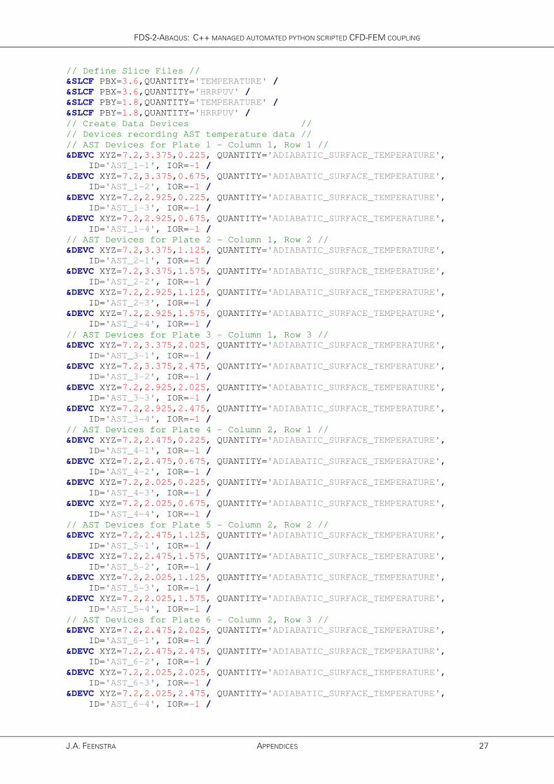
FDS-2-ABAQUS: C++ MANAGED AUTOMATED PYTHON SCRIPTED CFD-FEM COUPLING
J.A. FEENSTRA APPENDICES 27
// Define Slice Files //
&SLCF PBX=3.6,QUANTITY='TEMPERATURE' /
&SLCF PBX=3.6,QUANTITY='HRRPUV' /
&SLCF PBY=1.8,QUANTITY='TEMPERATURE' /
&SLCF PBY=1.8,QUANTITY='HRRPUV' /
// Create Data Devices //
// Devices recording AST temperature data //
// AST Devices for Plate 1 - Column 1, Row 1 //
&DEVC XYZ=7.2,3.375,0.225, QUANTITY='ADIABATIC_SURFACE_TEMPERATURE',
ID='AST_1-1', IOR=-1 /
&DEVC XYZ=7.2,3.375,0.675, QUANTITY='ADIABATIC_SURFACE_TEMPERATURE',
ID='AST_1-2', IOR=-1 /
&DEVC XYZ=7.2,2.925,0.225, QUANTITY='ADIABATIC_SURFACE_TEMPERATURE',
ID='AST_1-3', IOR=-1 /
&DEVC XYZ=7.2,2.925,0.675, QUANTITY='ADIABATIC_SURFACE_TEMPERATURE',
ID='AST_1-4', IOR=-1 /
// AST Devices for Plate 2 - Column 1, Row 2 //
&DEVC XYZ=7.2,3.375,1.125, QUANTITY='ADIABATIC_SURFACE_TEMPERATURE',
ID='AST_2-1', IOR=-1 /
&DEVC XYZ=7.2,3.375,1.575, QUANTITY='ADIABATIC_SURFACE_TEMPERATURE',
ID='AST_2-2', IOR=-1 /
&DEVC XYZ=7.2,2.925,1.125, QUANTITY='ADIABATIC_SURFACE_TEMPERATURE',
ID='AST_2-3', IOR=-1 /
&DEVC XYZ=7.2,2.925,1.575, QUANTITY='ADIABATIC_SURFACE_TEMPERATURE',
ID='AST_2-4', IOR=-1 /
// AST Devices for Plate 3 - Column 1, Row 3 //
&DEVC XYZ=7.2,3.375,2.025, QUANTITY='ADIABATIC_SURFACE_TEMPERATURE',
ID='AST_3-1', IOR=-1 /
&DEVC XYZ=7.2,3.375,2.475, QUANTITY='ADIABATIC_SURFACE_TEMPERATURE',
ID='AST_3-2', IOR=-1 /
&DEVC XYZ=7.2,2.925,2.025, QUANTITY='ADIABATIC_SURFACE_TEMPERATURE',
ID='AST_3-3', IOR=-1 /
&DEVC XYZ=7.2,2.925,2.475, QUANTITY='ADIABATIC_SURFACE_TEMPERATURE',
ID='AST_3-4', IOR=-1 /
// AST Devices for Plate 4 - Column 2, Row 1 //
&DEVC XYZ=7.2,2.475,0.225, QUANTITY='ADIABATIC_SURFACE_TEMPERATURE',
ID='AST_4-1', IOR=-1 /
&DEVC XYZ=7.2,2.475,0.675, QUANTITY='ADIABATIC_SURFACE_TEMPERATURE',
ID='AST_4-2', IOR=-1 /
&DEVC XYZ=7.2,2.025,0.225, QUANTITY='ADIABATIC_SURFACE_TEMPERATURE',
ID='AST_4-3', IOR=-1 /
&DEVC XYZ=7.2,2.025,0.675, QUANTITY='ADIABATIC_SURFACE_TEMPERATURE',
ID='AST_4-4', IOR=-1 /
// AST Devices for Plate 5 - Column 2, Row 2 //
&DEVC XYZ=7.2,2.475,1.125, QUANTITY='ADIABATIC_SURFACE_TEMPERATURE',
ID='AST_5-1', IOR=-1 /
&DEVC XYZ=7.2,2.475,1.575, QUANTITY='ADIABATIC_SURFACE_TEMPERATURE',
ID='AST_5-2', IOR=-1 /
&DEVC XYZ=7.2,2.025,1.125, QUANTITY='ADIABATIC_SURFACE_TEMPERATURE',
ID='AST_5-3', IOR=-1 /
&DEVC XYZ=7.2,2.025,1.575, QUANTITY='ADIABATIC_SURFACE_TEMPERATURE',
ID='AST_5-4', IOR=-1 /
// AST Devices for Plate 6 - Column 2, Row 3 //
&DEVC XYZ=7.2,2.475,2.025, QUANTITY='ADIABATIC_SURFACE_TEMPERATURE',
ID='AST_6-1', IOR=-1 /
&DEVC XYZ=7.2,2.475,2.475, QUANTITY='ADIABATIC_SURFACE_TEMPERATURE',
ID='AST_6-2', IOR=-1 /
&DEVC XYZ=7.2,2.025,2.025, QUANTITY='ADIABATIC_SURFACE_TEMPERATURE',
ID='AST_6-3', IOR=-1 /
&DEVC XYZ=7.2,2.025,2.475, QUANTITY='ADIABATIC_SURFACE_TEMPERATURE',
ID='AST_6-4', IOR=-1 /
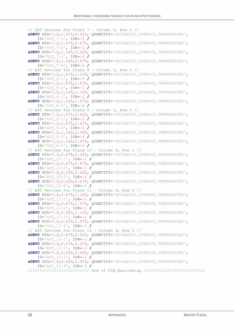
ADDITIONALLY ASSESSING TWO-WAY COUPLING EFFECTIVENESS
28 APPENDICES MASTER THESIS
// AST Devices for Plate 7 - Column 3, Row 1 //
&DEVC XYZ=7.2,1.575,0.225, QUANTITY='ADIABATIC_SURFACE_TEMPERATURE',
ID='AST_7-1', IOR=-1 /
&DEVC XYZ=7.2,1.575,0.675, QUANTITY='ADIABATIC_SURFACE_TEMPERATURE',
ID='AST_7-2', IOR=-1 /
&DEVC XYZ=7.2,1.125,0.225, QUANTITY='ADIABATIC_SURFACE_TEMPERATURE',
ID='AST_7-3', IOR=-1 /
&DEVC XYZ=7.2,1.125,0.675, QUANTITY='ADIABATIC_SURFACE_TEMPERATURE',
ID='AST_7-4', IOR=-1 /
// AST Devices for Plate 8 - Column 3, Row 2 //
&DEVC XYZ=7.2,1.575,1.125, QUANTITY='ADIABATIC_SURFACE_TEMPERATURE',
ID='AST_8-1', IOR=-1 /
&DEVC XYZ=7.2,1.575,1.575, QUANTITY='ADIABATIC_SURFACE_TEMPERATURE',
ID='AST_8-2', IOR=-1 /
&DEVC XYZ=7.2,1.125,1.125, QUANTITY='ADIABATIC_SURFACE_TEMPERATURE',
ID='AST_8-3', IOR=-1 /
&DEVC XYZ=7.2,1.125,1.575, QUANTITY='ADIABATIC_SURFACE_TEMPERATURE',
ID='AST_8-4', IOR=-1 /
// AST Devices for Plate 9 - Column 3, Row 3 //
&DEVC XYZ=7.2,1.575,2.025, QUANTITY='ADIABATIC_SURFACE_TEMPERATURE',
ID='AST_9-1', IOR=-1 /
&DEVC XYZ=7.2,1.575,2.475, QUANTITY='ADIABATIC_SURFACE_TEMPERATURE',
ID='AST_9-2', IOR=-1 /
&DEVC XYZ=7.2,1.125,2.025, QUANTITY='ADIABATIC_SURFACE_TEMPERATURE',
ID='AST_9-3', IOR=-1 /
&DEVC XYZ=7.2,1.125,2.475, QUANTITY='ADIABATIC_SURFACE_TEMPERATURE',
ID='AST_9-4', IOR=-1 /
// AST Devices for Plate 10 - Column 4, Row 1 //
&DEVC XYZ=7.2,0.675,0.225, QUANTITY='ADIABATIC_SURFACE_TEMPERATURE',
ID='AST_10-1', IOR=-1 /
&DEVC XYZ=7.2,0.675,0.675, QUANTITY='ADIABATIC_SURFACE_TEMPERATURE',
ID='AST_10-2', IOR=-1 /
&DEVC XYZ=7.2,0.225,0.225, QUANTITY='ADIABATIC_SURFACE_TEMPERATURE',
ID='AST_10-3', IOR=-1 /
&DEVC XYZ=7.2,0.225,0.675, QUANTITY='ADIABATIC_SURFACE_TEMPERATURE',
ID='AST_10-4', IOR=-1 /
// AST Devices for Plate 11 - Column 4, Row 2 //
&DEVC XYZ=7.2,0.675,1.125, QUANTITY='ADIABATIC_SURFACE_TEMPERATURE',
ID='AST_11-1', IOR=-1 /
&DEVC XYZ=7.2,0.675,1.575, QUANTITY='ADIABATIC_SURFACE_TEMPERATURE',
ID='AST_11-2', IOR=-1 /
&DEVC XYZ=7.2,0.225,1.125, QUANTITY='ADIABATIC_SURFACE_TEMPERATURE',
ID='AST_11-3', IOR=-1 /
&DEVC XYZ=7.2,0.225,1.575, QUANTITY='ADIABATIC_SURFACE_TEMPERATURE',
ID='AST_11-4', IOR=-1 /
// AST Devices for Plate 12 - Column 4, Row 3 //
&DEVC XYZ=7.2,0.675,2.025, QUANTITY='ADIABATIC_SURFACE_TEMPERATURE',
ID='AST_12-1', IOR=-1 /
&DEVC XYZ=7.2,0.675,2.475, QUANTITY='ADIABATIC_SURFACE_TEMPERATURE',
ID='AST_12-2', IOR=-1 /
&DEVC XYZ=7.2,0.225,2.025, QUANTITY='ADIABATIC_SURFACE_TEMPERATURE',
ID='AST_12-3', IOR=-1 /
&DEVC XYZ=7.2,0.225,2.475, QUANTITY='ADIABATIC_SURFACE_TEMPERATURE',
ID='AST_12-4', IOR=-1 /
////////////////////////// End of FDS_BasicSetup //////////////////////////
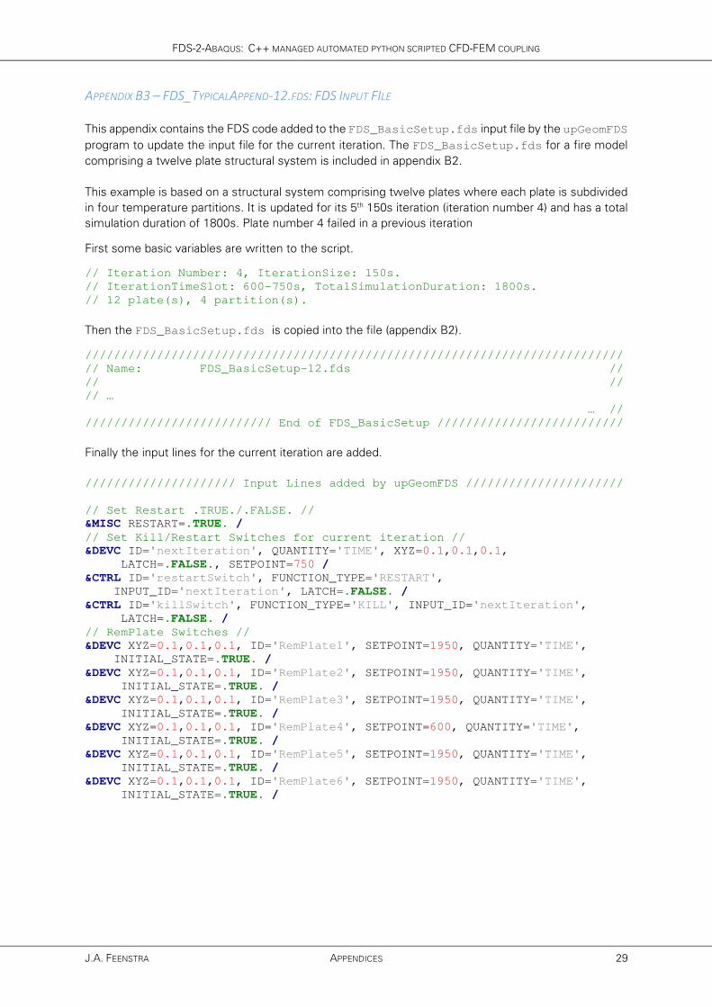
FDS-2-ABAQUS: C++ MANAGED AUTOMATED PYTHON SCRIPTED CFD-FEM COUPLING
J.A. FEENSTRA APPENDICES 29
APPENDIX B3 – FDS_TYPICALAPPEND-12.FDS: FDS INPUT FILE
This appendix contains the FDS code added to the FDS_BasicSetup.fds input file by the upGeomFDS
program to update the input file for the current iteration. The FDS_BasicSetup.fds for a fire model
comprising a twelve plate structural system is included in appendix B2.
This example is based on a structural system comprising twelve plates where each plate is subdivided
in four temperature partitions. It is updated for its 5th 150s iteration (iteration number 4) and has a total
simulation duration of 1800s. Plate number 4 failed in a previous iteration
First some basic variables are written to the script.
// Iteration Number: 4, IterationSize: 150s.
// IterationTimeSlot: 600-750s, TotalSimulationDuration: 1800s.
// 12 plate(s), 4 partition(s).
Then the FDS_BasicSetup.fds is copied into the file (appendix B2).
///////////////////////////////////////////////////////////////////////////
// Name: FDS_BasicSetup-12.fds //
// // // …
… //
////////////////////////// End of FDS_BasicSetup //////////////////////////
Finally the input lines for the current iteration are added.
///////////////////// Input Lines added by upGeomFDS //////////////////////
// Set Restart .TRUE./.FALSE. //
&MISC RESTART=.TRUE. /
// Set Kill/Restart Switches for current iteration //
&DEVC ID='nextIteration', QUANTITY='TIME', XYZ=0.1,0.1,0.1,
LATCH=.FALSE., SETPOINT=750 /
&CTRL ID='restartSwitch', FUNCTION_TYPE='RESTART',
INPUT_ID='nextIteration', LATCH=.FALSE. /
&CTRL ID='killSwitch', FUNCTION_TYPE='KILL', INPUT_ID='nextIteration',
LATCH=.FALSE. /
// RemPlate Switches //
&DEVC XYZ=0.1,0.1,0.1, ID='RemPlate1', SETPOINT=1950, QUANTITY='TIME',
INITIAL_STATE=.TRUE. /
&DEVC XYZ=0.1,0.1,0.1, ID='RemPlate2', SETPOINT=1950, QUANTITY='TIME',
INITIAL_STATE=.TRUE. /
&DEVC XYZ=0.1,0.1,0.1, ID='RemPlate3', SETPOINT=1950, QUANTITY='TIME',
INITIAL_STATE=.TRUE. /
&DEVC XYZ=0.1,0.1,0.1, ID='RemPlate4', SETPOINT=600, QUANTITY='TIME',
INITIAL_STATE=.TRUE. /
&DEVC XYZ=0.1,0.1,0.1, ID='RemPlate5', SETPOINT=1950, QUANTITY='TIME',
INITIAL_STATE=.TRUE. /
&DEVC XYZ=0.1,0.1,0.1, ID='RemPlate6', SETPOINT=1950, QUANTITY='TIME',
INITIAL_STATE=.TRUE. /
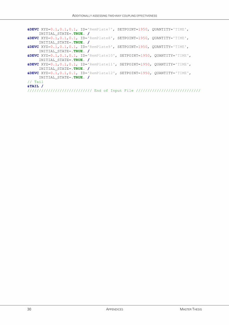
ADDITIONALLY ASSESSING TWO-WAY COUPLING EFFECTIVENESS
30 APPENDICES MASTER THESIS
&DEVC XYZ=0.1,0.1,0.1, ID='RemPlate7', SETPOINT=1950, QUANTITY='TIME',
INITIAL_STATE=.TRUE. /
&DEVC XYZ=0.1,0.1,0.1, ID='RemPlate8', SETPOINT=1950, QUANTITY='TIME',
INITIAL_STATE=.TRUE. /
&DEVC XYZ=0.1,0.1,0.1, ID='RemPlate9', SETPOINT=1950, QUANTITY='TIME',
INITIAL_STATE=.TRUE. /
&DEVC XYZ=0.1,0.1,0.1, ID='RemPlate10', SETPOINT=1950, QUANTITY='TIME',
INITIAL_STATE=.TRUE. /
&DEVC XYZ=0.1,0.1,0.1, ID='RemPlate11', SETPOINT=1950, QUANTITY='TIME',
INITIAL_STATE=.TRUE. /
&DEVC XYZ=0.1,0.1,0.1, ID='RemPlate12', SETPOINT=1950, QUANTITY='TIME',
INITIAL_STATE=.TRUE. /
// Tail
&TAIL /
//////////////////////////// End of Input File ////////////////////////////
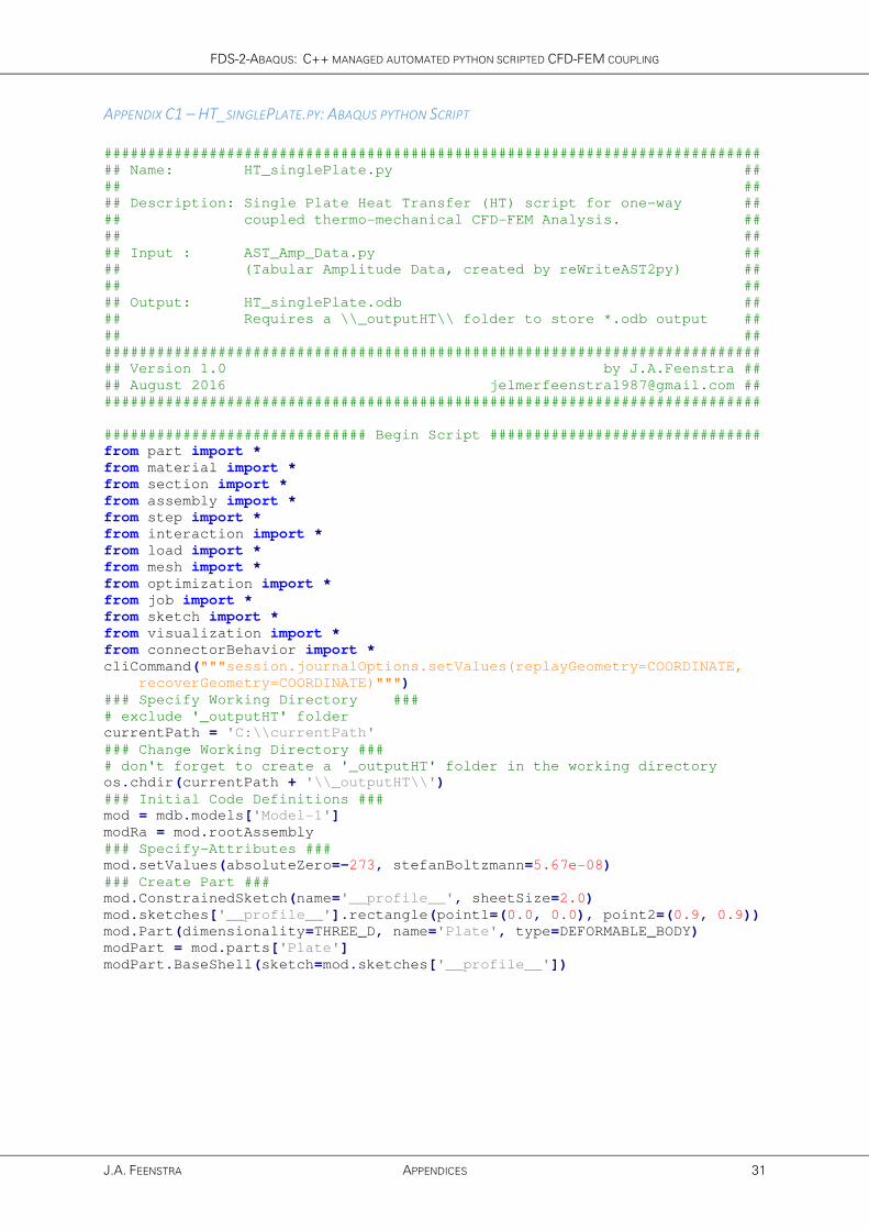
FDS-2-ABAQUS: C++ MANAGED AUTOMATED PYTHON SCRIPTED CFD-FEM COUPLING
J.A. FEENSTRA APPENDICES 31
APPENDIX C1 – HT_SINGLEPLATE.PY: ABAQUS PYTHON SCRIPT
###########################################################################
## Name: HT_singlePlate.py ##
## ##
## Description: Single Plate Heat Transfer (HT) script for one-way ##
## coupled thermo-mechanical CFD-FEM Analysis. ##
## ##
## Input : AST_Amp_Data.py ##
## (Tabular Amplitude Data, created by reWriteAST2py) ##
## ##
## Output: HT_singlePlate.odb ##
## Requires a \\_outputHT\\ folder to store *.odb output ##
## ##
###########################################################################
## Version 1.0 by J.A.Feenstra ##
## August 2016 [email protected] ##
###########################################################################
############################## Begin Script ###############################
from part import *
from material import *
from section import *
from assembly import *
from step import *
from interaction import *
from load import *
from mesh import *
from optimization import *
from job import *
from sketch import *
from visualization import *
from connectorBehavior import *
cliCommand("""session.journalOptions.setValues(replayGeometry=COORDINATE,
recoverGeometry=COORDINATE)""")
### Specify Working Directory ###
# exclude '_outputHT' folder
currentPath = 'C:\\currentPath'
### Change Working Directory ###
# don't forget to create a '_outputHT' folder in the working directory
os.chdir(currentPath + '\\_outputHT\\')
### Initial Code Definitions ###
mod = mdb.models['Model-1']
modRa = mod.rootAssembly
### Specify-Attributes ###
mod.setValues(absoluteZero=-273, stefanBoltzmann=5.67e-08)
### Create Part ###
mod.ConstrainedSketch(name='__profile__', sheetSize=2.0)
mod.sketches['__profile__'].rectangle(point1=(0.0, 0.0), point2=(0.9, 0.9))
mod.Part(dimensionality=THREE_D, name='Plate', type=DEFORMABLE_BODY)
modPart = mod.parts['Plate']
modPart.BaseShell(sketch=mod.sketches['__profile__'])

ADDITIONALLY ASSESSING TWO-WAY COUPLING EFFECTIVENESS
32 APPENDICES MASTER THESIS
### Create Sets ###
#Plate-Area, Edge-Top, Edge-Right, Edge-Bot, and Edge-Left
modPartFfa = modPart.faces.findAt
modPartEfa = modPart.edges.findAt
modPart.Set(faces=modPartFfa(((0.45, 0.45, 0.0),)), name='Plate-Area')
modPart.Set(edges=modPartEfa(((0.45, 0.9, 0.0), )), name='Edge-Top')
modPart.Set(edges=modPartEfa(((0.45, 0.0, 0.0), )), name='Edge-Bot')
modPart.Set(edges=modPartEfa(((0.0, 0.45, 0.0), )), name='Edge-Left')
modPart.Set(edges=modPartEfa(((0.9, 0.45, 0.0), )), name='Edge-Right')
modRa.regenerate()
### Create Partitions ###
modPartInPo = modPart.InterestingPoint
modPart.PartitionFaceByShortestPath(faces=modPartFfa(((0.3, 0.3, 0.0), )),
point1=modPartInPo(modPartEfa((0.675, 0.0, 0.0), ), MIDDLE),
point2=modPartInPo(modPartEfa((0.225, 0.9, 0.0), ), MIDDLE))
modPart.PartitionFaceByShortestPath(faces=modPartFfa(((0.3, 0.6, 0.0), )),
point1=modPartInPo(modPartEfa((0.0, 0.225, 0.0), ), MIDDLE),
point2=modPartInPo(modPartEfa((0.45, 0.675, 0.0), ), MIDDLE))
modPart.PartitionFaceByShortestPath(faces=modPartFfa(((0.6, 0.3, 0.0), )),
point1=modPart.vertices.findAt((0.45, 0.45, 0.0), ),
point2=modPartInPo(modPartEfa((0.9, 0.675, 0.0), ), MIDDLE))
### Create Surfaces ###
# Naming Convention
# 1)bottomLeft 2)topLeft 3)bottomRight 4)topRight
modPart.Surface(name='Surf-1', side1Faces=modPartFfa(((0.3, 0.3, 0.0), )))
modPart.Surface(name='Surf-2', side1Faces=modPartFfa(((0.15, 0.6, 0.0),)))
modPart.Surface(name='Surf-3', side1Faces=modPartFfa(((0.75, 0.3, 0.0),)))
modPart.Surface(name='Surf-4', side1Faces=modPartFfa(((0.6, 0.6, 0.0), )))
### Create Material ###
mod.Material(name='Steel')
modMat = mod.materials['Steel']
modMat.Elastic(table=((210000000000.0, 0.29),))
modMat.Density(table=((7850.0, ), ))
modMat.SpecificHeat(table=((452.0, ), ))
modMat.Conductivity(table=((53.3, ), ))
modMat.Expansion(table=((12e-06, ), ))
### Create Section ###
mod.HomogeneousShellSection(material='Steel', name='Section-Plate',
numIntPts=5, thickness=0.003)
### Assign Section ###
modPart.SectionAssignment(offset=0.0,
offsetField='', offsetType=MIDDLE_SURFACE, region=
modPart.sets['Plate-Area'], sectionName=
'Section-Plate', thicknessAssignment=FROM_SECTION)
### Create Instance ###
modRa.DatumCsysByDefault(CARTESIAN)
modRa.Instance(dependent=ON, name='Plate-1', part=modPart)
### Create Step ###
mod.HeatTransferStep(deltmx=50.0, initialInc=1E-6, maxInc=
10.0, maxNumInc=1000, minInc=1E-6, name='i0_HT-Step',
previous='Initial', timePeriod=3650.0)
### Import Adiabatic Temperature Data ###
imp = mod.TabularAmplitude
execfile(r'../AST_Amp_Data.py', __main__.__dict__)
### Request Field Output ###
# Field Output is requested every 5 seconds.
modFOR = mod.fieldOutputRequests['F-Output-1']
modFOR.setValues(variables=('NT',), timeInterval=5.0)
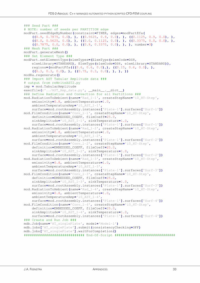
FDS-2-ABAQUS: C++ MANAGED AUTOMATED PYTHON SCRIPTED CFD-FEM COUPLING
J.A. FEENSTRA APPENDICES 33
### Seed Part ###
# NOTE: number of seeds per PARTITION edge
modPart.seedEdgeByNumber(constraint=FINER, edges=modPartEfa(
((0.9, 0.7875, 0.0), ), ((0.5625, 0.9, 0.0), ), ((0.1125, 0.9, 0.0), ),
((0.0, 0.5625, 0.0), ), ((0.0, 0.1125, 0.0), ), ((0.3375, 0.0, 0.0), ),
((0.7875, 0.0, 0.0), ), ((0.9, 0.3375, 0.0), ), ), number=3)
### Mesh Part ###
modPart.generateMesh()
### Set Element Type ###
modPart.setElementType(elemTypes=(ElemType(elemCode=DS8,
elemLibrary=STANDARD), ElemType(elemCode=DS6, elemLibrary=STANDARD)),
regions=(modPartFfa(((0.6, 0.6, 0.0),), ((0.15, 0.6, 0.0), ),
((0.3, 0.3, 0.0), ), ((0.75, 0.3, 0.0), ), ), ))
modRa.regenerate()
### Import AST Tabular Amplitude data ###
# output from reWriteAST2.py
imp = mod.TabularAmplitude
execfile(r'../AST_Amp_data.py', __main__.__dict__)
### Define Radiation and Convection for all Partitions ###
mod.RadiationToAmbient(name='Rad_1-1', createStepName='i0_HT-Step',
emissivity=0.8, ambientTemperature=1.0,
ambientTemperatureAmp='i0_AST_1-1',
surface=mod.rootAssembly.instances['Plate-1'].surfaces['Surf-1'])
mod.FilmCondition(name='Conv_1-1', createStepName='i0_HT-Step',
definition=EMBEDDED_COEFF, filmCoeff=25.0,
sinkAmplitude='i0_AST_1-1', sinkTemperature=1.0,
surface=mod.rootAssembly.instances['Plate-1'].surfaces['Surf-1'])
mod.RadiationToAmbient(name='Rad_1-2', createStepName='i0_HT-Step',
emissivity=0.8, ambientTemperature=1.0,
ambientTemperatureAmp='i0_AST_1-2',
surface=mod.rootAssembly.instances['Plate-1'].surfaces['Surf-2'])
mod.FilmCondition(name='Conv_1-2', createStepName='i0_HT-Step',
definition=EMBEDDED_COEFF, filmCoeff=25.0,
sinkAmplitude='i0_AST_1-2', sinkTemperature=1.0,
surface=mod.rootAssembly.instances['Plate-1'].surfaces['Surf-2'])
mod.RadiationToAmbient(name='Rad_1-3', createStepName='i0_HT-Step',
emissivity=0.8, ambientTemperature=1.0,
ambientTemperatureAmp='i0_AST_1-3',
surface=mod.rootAssembly.instances['Plate-1'].surfaces['Surf-3'])
mod.FilmCondition(name='Conv_1-3', createStepName='i0_HT-Step',
definition=EMBEDDED_COEFF, filmCoeff=25.0,
sinkAmplitude='i0_AST_1-3', sinkTemperature=1.0,
surface=mod.rootAssembly.instances['Plate-1'].surfaces['Surf-3'])
mod.RadiationToAmbient(name='Rad_1-4', createStepName='i0_HT-Step',
emissivity=0.8, ambientTemperature=1.0,
ambientTemperatureAmp='i0_AST_1-4',
surface=mod.rootAssembly.instances['Plate-1'].surfaces['Surf-4'])
mod.FilmCondition(name='Conv_1-4', createStepName='i0_HT-Step',
definition=EMBEDDED_COEFF, filmCoeff=25.0,
sinkAmplitude='i0_AST_1-4', sinkTemperature=1.0,
surface=mod.rootAssembly.instances['Plate-1'].surfaces['Surf-4'])
### Create and Run Job ###
mdb.Job(name='HT_singlePlate', model='Model-1')
mdb.jobs['HT_singlePlate'].submit(consistencyChecking=OFF)
mdb.jobs['HT_singlePlate'].waitForCompletion()
############################## End-Of-Script ##############################


FDS-2-ABAQUS: C++ MANAGED AUTOMATED PYTHON SCRIPTED CFD-FEM COUPLING
J.A. FEENSTRA APPENDICES 35
APPENDIX C2 – HT_BASICMODEL-12.PY: ABAQUS PYTHON SCRIPT
###########################################################################
## Name: HT_basicModel-12.py ##
## ##
## Description: Basic Heat Transfer (HT) Model for a 12 plate thin ##
## walled steel facade for use in two-way coupled thermo- ##
## mechanical CFD-FEM Analysis. ##
## ##
## Additional This script is INCOMPLETE additional python code is ##
## Info: appended by geometric update program upGeomHT based on ##
## the current iteration and failure progression. ##
## The complete coupling procedure is managed by ##
## Master Program FDS-2-Abaqus. ##
## ##
## Input : AST_Amp_Data.py ##
## (code calling this script is appended by upGeomHT) ##
## ##
## Output: HT_Script.odb ##
## Requires a \\_outputHT\\ folder to store *.odb output ##
## ##
###########################################################################
## Version 1.0 by J.A.Feenstra ##
## August 2016 [email protected] ##
###########################################################################
############################## Begin Script ###############################
from part import *
from material import *
from section import *
from assembly import *
from step import *
from interaction import *
from load import *
from mesh import *
from optimization import *
from job import *
from sketch import *
from visualization import *
from connectorBehavior import *
cliCommand("""session.journalOptions.setValues(replayGeometry=COORDINATE,
recoverGeometry=COORDINATE)""")
### Specify Working Directory ###
# exclude '_outputSR' folder
# use this line for use in FDS-2-Abaqus (relative path)
## currentPath = os.getcwd() # use this
# use this line when running script from Abaqus CEA (direct path)
currentPath = 'C:\\currentPath' # or this
# don't forget to create a '_outputHT' folder in the working directory
### Change Working Directory ###
os.chdir(currentPath + '\\_outputHT\\')
### Initial Code Definitions ###
mod = mdb.models['Model-1']
modRa = mod.rootAssembly
### Specify-Attributes ###
mod.setValues(absoluteZero=-273, stefanBoltzmann=5.67e-08)

ADDITIONALLY ASSESSING TWO-WAY COUPLING EFFECTIVENESS
36 APPENDICES MASTER THESIS
### Create Part ###
mod.ConstrainedSketch(name='__profile__', sheetSize=2.0)
mod.sketches['__profile__'].rectangle(point1=(0.0, 0.0), point2=(0.9, 0.9))
mod.Part(dimensionality=THREE_D, name='Plate', type=DEFORMABLE_BODY)
modPart = mod.parts['Plate']
modPart.BaseShell(sketch=mod.sketches['__profile__'])
### Create Sets ###
#Plate-Area, Edge-Top, Edge-Right, Edge-Bot, and Edge-Left
modPartFfa = modPart.faces.findAt
modPartEfa = modPart.edges.findAt
modPart.Set(faces=modPartFfa(((0.45, 0.45, 0.0),)), name='Plate-Area')
modPart.Set(edges=modPartEfa(((0.45, 0.9, 0.0), )), name='Edge-Top')
modPart.Set(edges=modPartEfa(((0.45, 0.0, 0.0), )), name='Edge-Bot')
modPart.Set(edges=modPartEfa(((0.0, 0.45, 0.0), )), name='Edge-Left')
modPart.Set(edges=modPartEfa(((0.9, 0.45, 0.0), )), name='Edge-Right')
modRa.regenerate()
### Create Partitions ###
modPartInPo = modPart.InterestingPoint
modPart.PartitionFaceByShortestPath(faces=modPartFfa(((0.3, 0.3, 0.0), )),
point1=modPartInPo(modPartEfa((0.675, 0.0, 0.0), ), MIDDLE),
point2=modPartInPo(modPartEfa((0.225, 0.9, 0.0), ), MIDDLE))
modPart.PartitionFaceByShortestPath(faces=modPartFfa(((0.3, 0.6, 0.0), )),
point1=modPartInPo(modPartEfa((0.0, 0.225, 0.0), ), MIDDLE),
point2=modPartInPo(modPartEfa((0.45, 0.675, 0.0), ), MIDDLE))
modPart.PartitionFaceByShortestPath(faces=modPartFfa(((0.6, 0.3, 0.0), )),
point1=modPart.vertices.findAt((0.45, 0.45, 0.0), ),
point2=modPartInPo(modPartEfa((0.9, 0.675, 0.0), ), MIDDLE))
### Create Surfaces ###
# Naming Convention
# 1)bottomLeft 2)topLeft 3)bottomRight 4)topRight
modPart.Surface(name='Surf-1', side1Faces=modPartFfa(((0.3, 0.3, 0.0), )))
modPart.Surface(name='Surf-2', side1Faces=modPartFfa(((0.15, 0.6, 0.0),)))
modPart.Surface(name='Surf-3', side1Faces=modPartFfa(((0.75, 0.3, 0.0),)))
modPart.Surface(name='Surf-4', side1Faces=modPartFfa(((0.6, 0.6, 0.0), )))
### Create Material ###
mod.Material(name='Steel')
modMat = mod.materials['Steel']
modMat.Elastic(table=((210000000000.0, 0.29),))
modMat.Density(table=((7850.0, ), ))
modMat.SpecificHeat(table=((452.0, ), ))
modMat.Conductivity(table=((53.3, ), ))
modMat.Expansion(table=((12e-06, ), ))
### Create Section ###
mod.HomogeneousShellSection(material='Steel', name='Section-Plate',
numIntPts=5, thickness=0.003)
### Assign Section ###
modPart.SectionAssignment(offset=0.0,
offsetField='', offsetType=MIDDLE_SURFACE, region=
modPart.sets['Plate-Area'], sectionName=
'Section-Plate', thicknessAssignment=FROM_SECTION)
### Create Instance ###
modRa.DatumCsysByDefault(CARTESIAN)
modRa.Instance(dependent=ON, name='Plate-1', part=modPart)
### Pattern Multiple Instances ###
modRa.LinearInstancePattern(instanceList=('Plate-1', ),
direction1=(1.0, 0.0, 0.0), direction2=(0.0, 1.0, 0.0),
number1=4, number2=3, spacing1=0.9, spacing2=0.9)
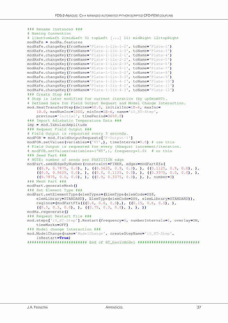
FDS-2-ABAQUS: C++ MANAGED AUTOMATED PYTHON SCRIPTED CFD-FEM COUPLING
J.A. FEENSTRA APPENDICES 37
### Rename Instances ###
# Naming Convention
# 1)bottomLeft 2)midLeft 3) topLeft [...] 11) midRight 12)topRight
modRaFe = modRa.features
modRaFe.changeKey(fromName='Plate-1-lin-1-2', toName='Plate-2')
modRaFe.changeKey(fromName='Plate-1-lin-1-3', toName='Plate-3')
modRaFe.changeKey(fromName='Plate-1-lin-2-1', toName='Plate-4')
modRaFe.changeKey(fromName='Plate-1-lin-2-2', toName='Plate-5')
modRaFe.changeKey(fromName='Plate-1-lin-2-3', toName='Plate-6')
modRaFe.changeKey(fromName='Plate-1-lin-3-1', toName='Plate-7')
modRaFe.changeKey(fromName='Plate-1-lin-3-2', toName='Plate-8')
modRaFe.changeKey(fromName='Plate-1-lin-3-3', toName='Plate-9')
modRaFe.changeKey(fromName='Plate-1-lin-4-1', toName='Plate-10')
modRaFe.changeKey(fromName='Plate-1-lin-4-2', toName='Plate-11')
modRaFe.changeKey(fromName='Plate-1-lin-4-3', toName='Plate-12')
### Create Step ###
# Step is later modified for current iteration (by upGeomHT).
# Defined here for Field Output Request and Model Change Interaction.
mod.HeatTransferStep(deltmx=50.0, initialInc=1E-6, maxInc=
10.0, maxNumInc=1000, minInc=1E-6, name='i0_HT-Step',
previous='Initial', timePeriod=3650.0)
### Import Adiabatic Temperature Data ###
imp = mod.TabularAmplitude
### Request Field Output ###
# Field Output is requested every 5 seconds.
modFOR = mod.fieldOutputRequests['F-Output-1']
modFOR.setValues(variables=('NT',), timeInterval=5.0) # use this
# Field Output is requested for every (Abaqus) increment/iteration.
# modFOR.setValues(variables=('NT',), frequency=1.0) # or this
### Seed Part ###
# NOTE: number of seeds per PARTITION edge
modPart.seedEdgeByNumber(constraint=FINER, edges=modPartEfa(
((0.9, 0.7875, 0.0), ), ((0.5625, 0.9, 0.0), ), ((0.1125, 0.9, 0.0), ),
((0.0, 0.5625, 0.0), ), ((0.0, 0.1125, 0.0), ), ((0.3375, 0.0, 0.0), ),
((0.7875, 0.0, 0.0), ), ((0.9, 0.3375, 0.0), ), ), number=3)
### Mesh Part ###
modPart.generateMesh()
### Set Element Type ###
modPart.setElementType(elemTypes=(ElemType(elemCode=DS8,
elemLibrary=STANDARD), ElemType(elemCode=DS6, elemLibrary=STANDARD)),
regions=(modPartFfa(((0.6, 0.6, 0.0),), ((0.15, 0.6, 0.0), ),
((0.3, 0.3, 0.0), ), ((0.75, 0.3, 0.0), ), ), ))
modRa.regenerate()
### Request Restart File ###
mod.steps['i0_HT-Step'].Restart(frequency=0, numberIntervals=1, overlay=ON,
timeMarks=OFF)
### Model change Interaction ###
mod.ModelChange(name='ModelChange', createStepName='i0_HT-Step',
isRestart=True)
########################## End of HT_basicModel ###########################

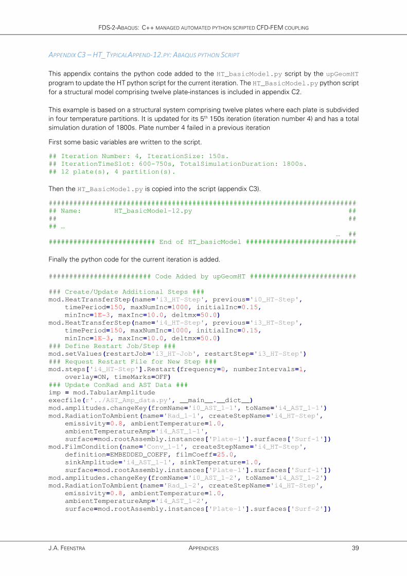
FDS-2-ABAQUS: C++ MANAGED AUTOMATED PYTHON SCRIPTED CFD-FEM COUPLING
J.A. FEENSTRA APPENDICES 39
APPENDIX C3 – HT_TYPICALAPPEND-12.PY: ABAQUS PYTHON SCRIPT
This appendix contains the python code added to the HT_basicModel.py script by the upGeomHT
program to update the HT python script for the current iteration. The HT_BasicModel.py python script
for a structural model comprising twelve plate-instances is included in appendix C2.
This example is based on a structural system comprising twelve plates where each plate is subdivided
in four temperature partitions. It is updated for its 5th 150s iteration (iteration number 4) and has a total
simulation duration of 1800s. Plate number 4 failed in a previous iteration
First some basic variables are written to the script.
## Iteration Number: 4, IterationSize: 150s.
## IterationTimeSlot: 600-750s, TotalSimulationDuration: 1800s.
## 12 plate(s), 4 partition(s).
Then the HT_BasicModel.py is copied into the script (appendix C3).
###########################################################################
## Name: HT_basicModel-12.py ##
## ##
## …
… ##
########################## End of HT_basicModel ###########################
Finally the python code for the current iteration is added.
######################### Code Added by upGeomHT ##########################
### Create/Update Additional Steps ###
mod.HeatTransferStep(name='i3_HT-Step', previous='i0_HT-Step',
timePeriod=150, maxNumInc=1000, initialInc=0.15,
minInc=1E-3, maxInc=10.0, deltmx=50.0)
mod.HeatTransferStep(name='i4_HT-Step', previous='i3_HT-Step',
timePeriod=150, maxNumInc=1000, initialInc=0.15,
minInc=1E-3, maxInc=10.0, deltmx=50.0)
### Define Restart Job/Step ###
mod.setValues(restartJob='i3_HT-Job', restartStep='i3_HT-Step')
### Request Restart File for New Step ###
mod.steps['i4_HT-Step'].Restart(frequency=0, numberIntervals=1,
overlay=ON, timeMarks=OFF)
### Update ConRad and AST Data ###
imp = mod.TabularAmplitude
execfile(r'../AST_Amp_data.py', __main__.__dict__)
mod.amplitudes.changeKey(fromName='i0_AST_1-1', toName='i4_AST_1-1')
mod.RadiationToAmbient(name='Rad_1-1', createStepName='i4_HT-Step',
emissivity=0.8, ambientTemperature=1.0,
ambientTemperatureAmp='i4_AST_1-1',
surface=mod.rootAssembly.instances['Plate-1'].surfaces['Surf-1'])
mod.FilmCondition(name='Conv_1-1', createStepName='i4_HT-Step',
definition=EMBEDDED_COEFF, filmCoeff=25.0,
sinkAmplitude='i4_AST_1-1', sinkTemperature=1.0,
surface=mod.rootAssembly.instances['Plate-1'].surfaces['Surf-1'])
mod.amplitudes.changeKey(fromName='i0_AST_1-2', toName='i4_AST_1-2')
mod.RadiationToAmbient(name='Rad_1-2', createStepName='i4_HT-Step',
emissivity=0.8, ambientTemperature=1.0,
ambientTemperatureAmp='i4_AST_1-2',
surface=mod.rootAssembly.instances['Plate-1'].surfaces['Surf-2'])
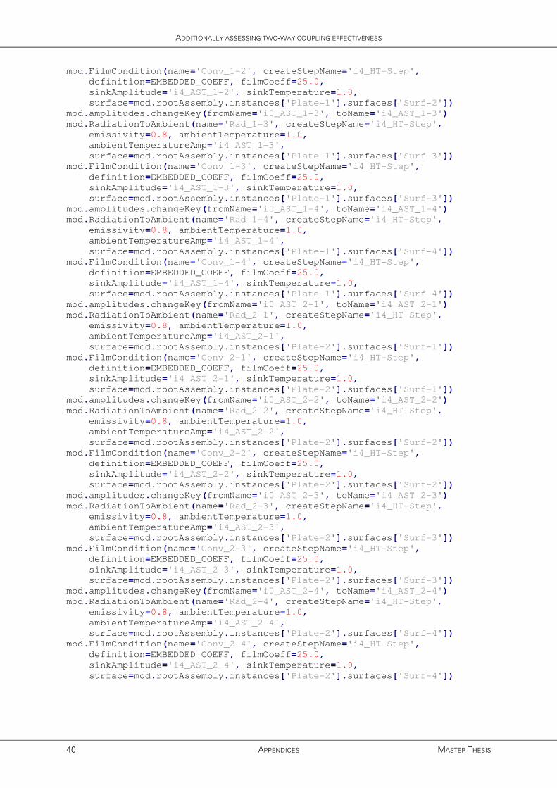
ADDITIONALLY ASSESSING TWO-WAY COUPLING EFFECTIVENESS
40 APPENDICES MASTER THESIS
mod.FilmCondition(name='Conv_1-2', createStepName='i4_HT-Step',
definition=EMBEDDED_COEFF, filmCoeff=25.0,
sinkAmplitude='i4_AST_1-2', sinkTemperature=1.0,
surface=mod.rootAssembly.instances['Plate-1'].surfaces['Surf-2'])
mod.amplitudes.changeKey(fromName='i0_AST_1-3', toName='i4_AST_1-3')
mod.RadiationToAmbient(name='Rad_1-3', createStepName='i4_HT-Step',
emissivity=0.8, ambientTemperature=1.0,
ambientTemperatureAmp='i4_AST_1-3',
surface=mod.rootAssembly.instances['Plate-1'].surfaces['Surf-3'])
mod.FilmCondition(name='Conv_1-3', createStepName='i4_HT-Step',
definition=EMBEDDED_COEFF, filmCoeff=25.0,
sinkAmplitude='i4_AST_1-3', sinkTemperature=1.0,
surface=mod.rootAssembly.instances['Plate-1'].surfaces['Surf-3'])
mod.amplitudes.changeKey(fromName='i0_AST_1-4', toName='i4_AST_1-4')
mod.RadiationToAmbient(name='Rad_1-4', createStepName='i4_HT-Step',
emissivity=0.8, ambientTemperature=1.0,
ambientTemperatureAmp='i4_AST_1-4',
surface=mod.rootAssembly.instances['Plate-1'].surfaces['Surf-4'])
mod.FilmCondition(name='Conv_1-4', createStepName='i4_HT-Step',
definition=EMBEDDED_COEFF, filmCoeff=25.0,
sinkAmplitude='i4_AST_1-4', sinkTemperature=1.0,
surface=mod.rootAssembly.instances['Plate-1'].surfaces['Surf-4'])
mod.amplitudes.changeKey(fromName='i0_AST_2-1', toName='i4_AST_2-1')
mod.RadiationToAmbient(name='Rad_2-1', createStepName='i4_HT-Step',
emissivity=0.8, ambientTemperature=1.0,
ambientTemperatureAmp='i4_AST_2-1',
surface=mod.rootAssembly.instances['Plate-2'].surfaces['Surf-1'])
mod.FilmCondition(name='Conv_2-1', createStepName='i4_HT-Step',
definition=EMBEDDED_COEFF, filmCoeff=25.0,
sinkAmplitude='i4_AST_2-1', sinkTemperature=1.0,
surface=mod.rootAssembly.instances['Plate-2'].surfaces['Surf-1'])
mod.amplitudes.changeKey(fromName='i0_AST_2-2', toName='i4_AST_2-2')
mod.RadiationToAmbient(name='Rad_2-2', createStepName='i4_HT-Step',
emissivity=0.8, ambientTemperature=1.0,
ambientTemperatureAmp='i4_AST_2-2',
surface=mod.rootAssembly.instances['Plate-2'].surfaces['Surf-2'])
mod.FilmCondition(name='Conv_2-2', createStepName='i4_HT-Step',
definition=EMBEDDED_COEFF, filmCoeff=25.0,
sinkAmplitude='i4_AST_2-2', sinkTemperature=1.0,
surface=mod.rootAssembly.instances['Plate-2'].surfaces['Surf-2'])
mod.amplitudes.changeKey(fromName='i0_AST_2-3', toName='i4_AST_2-3')
mod.RadiationToAmbient(name='Rad_2-3', createStepName='i4_HT-Step',
emissivity=0.8, ambientTemperature=1.0,
ambientTemperatureAmp='i4_AST_2-3',
surface=mod.rootAssembly.instances['Plate-2'].surfaces['Surf-3'])
mod.FilmCondition(name='Conv_2-3', createStepName='i4_HT-Step',
definition=EMBEDDED_COEFF, filmCoeff=25.0,
sinkAmplitude='i4_AST_2-3', sinkTemperature=1.0,
surface=mod.rootAssembly.instances['Plate-2'].surfaces['Surf-3'])
mod.amplitudes.changeKey(fromName='i0_AST_2-4', toName='i4_AST_2-4')
mod.RadiationToAmbient(name='Rad_2-4', createStepName='i4_HT-Step',
emissivity=0.8, ambientTemperature=1.0,
ambientTemperatureAmp='i4_AST_2-4',
surface=mod.rootAssembly.instances['Plate-2'].surfaces['Surf-4'])
mod.FilmCondition(name='Conv_2-4', createStepName='i4_HT-Step',
definition=EMBEDDED_COEFF, filmCoeff=25.0,
sinkAmplitude='i4_AST_2-4', sinkTemperature=1.0,
surface=mod.rootAssembly.instances['Plate-2'].surfaces['Surf-4'])

FDS-2-ABAQUS: C++ MANAGED AUTOMATED PYTHON SCRIPTED CFD-FEM COUPLING
J.A. FEENSTRA APPENDICES 41
###########################################################################
## Code for Plates 3 - 11 is excluded from this appendix ##
## for obvious reasons (Space, Ink, Paper!) ##
## (See also 'for loop' alternative below) ##
###########################################################################
mod.amplitudes.changeKey(fromName='i0_AST_12-1', toName='i4_AST_12-1')
mod.RadiationToAmbient(name='Rad_12-1', createStepName='i4_HT-Step',
emissivity=0.8, ambientTemperature=1.0,
ambientTemperatureAmp='i4_AST_12-1',
surface=mod.rootAssembly.instances['Plate-12'].surfaces['Surf-1'])
mod.FilmCondition(name='Conv_12-1', createStepName='i4_HT-Step',
definition=EMBEDDED_COEFF, filmCoeff=25.0,
sinkAmplitude='i4_AST_12-1', sinkTemperature=1.0,
surface=mod.rootAssembly.instances['Plate-12'].surfaces['Surf-1'])
mod.amplitudes.changeKey(fromName='i0_AST_12-2', toName='i4_AST_12-2')
mod.RadiationToAmbient(name='Rad_12-2', createStepName='i4_HT-Step',
emissivity=0.8, ambientTemperature=1.0,
ambientTemperatureAmp='i4_AST_12-2',
surface=mod.rootAssembly.instances['Plate-12'].surfaces['Surf-2'])
mod.FilmCondition(name='Conv_12-2', createStepName='i4_HT-Step',
definition=EMBEDDED_COEFF, filmCoeff=25.0,
sinkAmplitude='i4_AST_12-2', sinkTemperature=1.0,
surface=mod.rootAssembly.instances['Plate-12'].surfaces['Surf-2'])
mod.amplitudes.changeKey(fromName='i0_AST_12-3', toName='i4_AST_12-3')
mod.RadiationToAmbient(name='Rad_12-3', createStepName='i4_HT-Step',
emissivity=0.8, ambientTemperature=1.0,
ambientTemperatureAmp='i4_AST_12-3',
surface=mod.rootAssembly.instances['Plate-12'].surfaces['Surf-3'])
mod.FilmCondition(name='Conv_12-3', createStepName='i4_HT-Step',
definition=EMBEDDED_COEFF, filmCoeff=25.0,
sinkAmplitude='i4_AST_12-3', sinkTemperature=1.0,
surface=mod.rootAssembly.instances['Plate-12'].surfaces['Surf-3'])
mod.amplitudes.changeKey(fromName='i0_AST_12-4', toName='i4_AST_12-4')
mod.RadiationToAmbient(name='Rad_12-4', createStepName='i4_HT-Step',
emissivity=0.8, ambientTemperature=1.0,
ambientTemperatureAmp='i4_AST_12-4',
surface=mod.rootAssembly.instances['Plate-12'].surfaces['Surf-4'])
mod.FilmCondition(name='Conv_12-4', createStepName='i4_HT-Step',
definition=EMBEDDED_COEFF, filmCoeff=25.0,
sinkAmplitude='i4_AST_12-4', sinkTemperature=1.0,
surface=mod.rootAssembly.instances['Plate-12'].surfaces['Surf-4'])
### Update Model Geometry ###
thisPlate = mod.rootAssembly.instances['Plate-4'].sets['Plate-Area']
mod.ModelChange(activeInStep=False, createStepName='i4_HT-Step',
includeStrain=False, name='deActPlate-4', region=thisPlate)
# If empty: No plates failed this iteration - Still Going Strong!
### Create and Run Job ###
mdb.Job(name='i4_HT-Job', model='Model-1', type=RESTART)
mdb.jobs['i4_HT-Job'].submit(consistencyChecking=OFF)
mdb.jobs['i4_HT-Job'].waitForCompletion()
############################## End-Of-Script ##############################
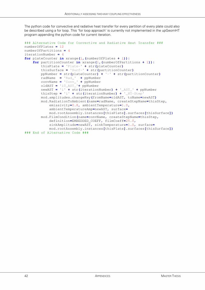
ADDITIONALLY ASSESSING TWO-WAY COUPLING EFFECTIVENESS
42 APPENDICES MASTER THESIS
The python code for convective and radiative heat transfer for every partition of every plate could also
be described using a for loop. This ‘for loop approach’ is currently not implemented in the upGeomHT
program appending the python code for current iteration.
### Alternative Code for Convective and Radiative Heat Transfer ###
numberOfPlates = 12
numberOfPartitions = 4
iterationNumber = 4
for plateCounter in xrange(1,(numberOfPlates + 1)):
for partitionCounter in xrange(1,(numberOfPartitions + 1)):
thisPlate = 'Plate-' + str(plateCounter)
thisSurface = 'Surf-' + str(partitionCounter)
ppNumber = str(plateCounter) + '-' + str(partitionCounter)
radName = 'Rad_' + ppNumber
convName = 'Conv_' + ppNumber
oldAST = 'i0_AST_'+ ppNumber
newAST = 'i' + str(iterationNumber) + '_AST_' + ppNumber
thisStep = 'i' + str(iterationNumber) + '_HT-Step'
mod.amplitudes.changeKey(fromName=oldAST, toName=newAST)
mod.RadiationToAmbient(name=radName, createStepName=thisStep,
emissivity=0.8, ambientTemperature=1.0,
ambientTemperatureAmp=newAST, surface=
mod.rootAssembly.instances[thisPlate].surfaces[thisSurface])
mod.FilmCondition(name=convName, createStepName=thisStep,
definition=EMBEDDED_COEFF, filmCoeff=25.0,
sinkAmplitude=newAST, sinkTemperature=1.0, surface=
mod.rootAssembly.instances[thisPlate].surfaces[thisSurface])
### End of Alternative Code ###
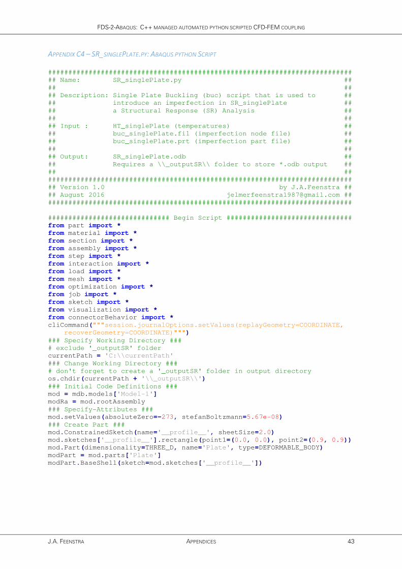
FDS-2-ABAQUS: C++ MANAGED AUTOMATED PYTHON SCRIPTED CFD-FEM COUPLING
J.A. FEENSTRA APPENDICES 43
APPENDIX C4 – SR_SINGLEPLATE.PY: ABAQUS PYTHON SCRIPT
###########################################################################
## Name: SR_singlePlate.py ##
## ##
## Description: Single Plate Buckling (buc) script that is used to ##
## introduce an imperfection in SR_singlePlate ##
## a Structural Response (SR) Analysis ##
## ##
## Input : HT_singlePlate (temperatures) ##
## buc_singlePlate.fil (imperfection node file) ##
## buc_singlePlate.prt (imperfection part file) ##
## ##
## Output: SR_singlePlate.odb ##
## Requires a \\_outputSR\\ folder to store *.odb output ##
## ##
###########################################################################
## Version 1.0 by J.A.Feenstra ##
## August 2016 [email protected] ##
###########################################################################
############################## Begin Script ###############################
from part import *
from material import *
from section import *
from assembly import *
from step import *
from interaction import *
from load import *
from mesh import *
from optimization import *
from job import *
from sketch import *
from visualization import *
from connectorBehavior import *
cliCommand("""session.journalOptions.setValues(replayGeometry=COORDINATE,
recoverGeometry=COORDINATE)""")
### Specify Working Directory ###
# exclude '_outputSR' folder
currentPath = 'C:\\currentPath'
### Change Working Directory ###
# don't forget to create a '_outputSR' folder in output directory
os.chdir(currentPath + '\\_outputSR\\')
### Initial Code Definitions ###
mod = mdb.models['Model-1']
modRa = mod.rootAssembly
### Specify-Attributes ###
mod.setValues(absoluteZero=-273, stefanBoltzmann=5.67e-08)
### Create Part ###
mod.ConstrainedSketch(name='__profile__', sheetSize=2.0)
mod.sketches['__profile__'].rectangle(point1=(0.0, 0.0), point2=(0.9, 0.9))
mod.Part(dimensionality=THREE_D, name='Plate', type=DEFORMABLE_BODY)
modPart = mod.parts['Plate']
modPart.BaseShell(sketch=mod.sketches['__profile__'])

ADDITIONALLY ASSESSING TWO-WAY COUPLING EFFECTIVENESS
44 APPENDICES MASTER THESIS
### Create Sets ###
#Plate-Area, Edge-Top, Edge-Right, Edge-Bot, and Edge-Left
modPartFfa = modPart.faces.findAt
modPartEfa = modPart.edges.findAt
modPart.Set(faces=modPartFfa(((0.45, 0.45, 0.0),)), name='Plate-Area')
modPart.Set(edges=modPartEfa(((0.45, 0.9, 0.0), )), name='Edge-Top')
modPart.Set(edges=modPartEfa(((0.45, 0.0, 0.0), )), name='Edge-Bot')
modPart.Set(edges=modPartEfa(((0.0, 0.45, 0.0), )), name='Edge-Left')
modPart.Set(edges=modPartEfa(((0.9, 0.45, 0.0), )), name='Edge-Right')
modRa.regenerate()
### Create Material ###
mod.Material(name='Steel')
modMat = mod.materials['Steel']
modMat.Elastic(table=((210000000000.0, 0.29),))
modMat.Density(table=((7850.0, ), ))
modMat.SpecificHeat(table=((452.0, ), ))
modMat.Conductivity(table=((53.3, ), ))
modMat.Expansion(table=((12e-06, ), ))
### Define Plasticity Material Property ### - S355
modMat.Plastic(table=((320000000.0, 0.0), (357000000.0, 0.002),
(366100000.0, 0.0157), (541600000.0, 0.1351)))
### Create Section ###
mod.HomogeneousShellSection(material='Steel', name='Section-Plate',
numIntPts=5, thickness=0.003)
### Assign Section ###
modPart.SectionAssignment(offset=0.0,
offsetField='', offsetType=MIDDLE_SURFACE, region=
modPart.sets['Plate-Area'], sectionName=
'Section-Plate', thicknessAssignment=FROM_SECTION)
### Create Instance ###
modRa.DatumCsysByDefault(CARTESIAN)
modRa.Instance(dependent=ON, name='Plate-1', part=modPart)
### Seed Part ###
modPart.seedEdgeByNumber(constraint=FINER, edges=
modPartEfa(((0.9, 0.7875, 0.0), ), ((0.5625, 0.9, 0.0), ),
((0.1125, 0.9, 0.0), ), ((0.0, 0.5625, 0.0), ), ((0.0, 0.1125, 0.0), ),
((0.3375, 0.0, 0.0), ), ((0.7875, 0.0, 0.0), ),
((0.9, 0.3375, 0.0), ), ), number=6)
### Mesh Part ###
modPart.generateMesh()
### Set Element Type ###
modPart.setElementType(elemTypes=(ElemType(elemCode=S8R,
elemLibrary=STANDARD), ElemType(elemCode=STRI65,
elemLibrary=STANDARD)), regions=(modPartFfa(((0.6, 0.6, 0.0),),
((0.15, 0.6, 0.0), ), ((0.3, 0.3, 0.0), ), ((0.75, 0.3, 0.0), ), ), ))
### Create-Step ###
mod.ImplicitDynamicsStep(name='i0_SR-Step', previous='Initial',
timePeriod=3650.0, maxNumInc=10000, application=QUASI_STATIC,
initialInc=0.3, minInc=1e-09, maxInc=25.0, nohaf=OFF, amplitude=RAMP,
alpha=DEFAULT, initialConditions=OFF, nlgeom=ON)
### Import Nodal Temperatures from HT ###
mod.Temperature(absoluteExteriorTolerance=0.0, beginIncrement=None,
beginStep=1, createStepName='i0_SR-Step', distributionType=FROM_FILE,
endIncrement=None, endStep=None, exteriorTolerance=0.05,
fileName='..\_outputHT\HT_singlePlate.odb', interpolate=ON,
name='i0_Temp-From-HT')

FDS-2-ABAQUS: C++ MANAGED AUTOMATED PYTHON SCRIPTED CFD-FEM COUPLING
J.A. FEENSTRA APPENDICES 45
### Request Field Output ###
# Field Output is requested every 5 seconds.
modFOR = mod.fieldOutputRequests['F-Output-1']
modFOR.setValues(timeInterval=5.0,
variables=('S','SSAVG', 'E', 'PE', 'PEEQ', 'U', 'NT', 'TEMP'))
## Create BCs ##
mod.DisplacementBC(createStepName='Initial', name='P1-BC-Top',
region=modRa.instances['Plate-1'].sets['Edge-Top'],
u1=SET, u2=SET, u3=SET, ur1=UNSET, ur2=UNSET, ur3=UNSET)
mod.DisplacementBC(createStepName='Initial', name='P1-BC-Bot',
region=modRa.instances['Plate-1'].sets['Edge-Bot'],
u1=SET, u2=SET, u3=SET, ur1=UNSET, ur2=UNSET, ur3=UNSET)
### Define Imperfection ###
mod.keywordBlock.synchVersions(storeNodesAndElements=False)
mod.keywordBlock.insert(38,
'\n*Imperfection, file=buc_singlePlate, step=1\n1, 0.003')
### Create and Run Job ###
mdb.Job(name='SR_singlePlate', model='Model-1')
mdb.jobs['SR_singlePlate'].submit(consistencyChecking=OFF)
mdb.jobs['SR_singlePlate'].waitForCompletion()
############################## End-Of-Script ##############################


FDS-2-ABAQUS: C++ MANAGED AUTOMATED PYTHON SCRIPTED CFD-FEM COUPLING
J.A. FEENSTRA APPENDICES 47
APPENDIX C5 – SR_BASICMODEL-12.PY: ABAQUS PYTHON SCRIPT
###########################################################################
## Name: SR_basicModel-12.py ##
## ##
## Description: Basic Structural Response (SR) Model for a 12 plate thin ##
## walled steel facade for use in two-way coupled thermo- ##
## mechanical CFD-FEM Analysis. ##
## ##
## Additional This script is INCOMPLETE additional python code is ##
## Info: appended by geometric update program upGeomSR based on ##
## the current iteration and failure progression. ##
## The complete coupling procedure is managed by ##
## Master Program FDS-2-Abaqus. ##
## ##
## Input : HT_Script.odb (temperatures) ##
## i0_buc-Job.fil (imperfection node file) ##
## i0_buc-Job.prt (imperfection part file) ##
## ##
## Output: SR_Script.odb ##
## Requires a \\_outputSR\\ folder to store *.odb output ##
## ##
###########################################################################
## Version 1.0 by J.A.Feenstra ##
## August 2016 [email protected] ##
###########################################################################
############################## Begin Script ###############################
from part import *
from material import *
from section import *
from assembly import *
from step import *
from interaction import *
from load import *
from mesh import *
from optimization import *
from job import *
from sketch import *
from visualization import *
from connectorBehavior import *
cliCommand("""session.journalOptions.setValues(replayGeometry=COORDINATE,
recoverGeometry=COORDINATE)""")
### Specify Working Directory ###
# exclude '_outputSR' folder
# use this line for use in FDS-2-Abaqus (relative path)
# currentPath = os.getcwd() # use this
# use this line when running script from Abaqus CEA (direct path)
currentPath = 'C:\\currentPath' # or this
# don't forget to create a '_outputSR' folder in the working directory
### Change Working Directory ###
# don't forget to create a '_outputSR' folder in output directory
os.chdir(currentPath + '\\_outputSR\\')
### Initial Code Definitions ###
mod = mdb.models['Model-1']
modRa = mod.rootAssembly
### Specify-Attributes ###
mod.setValues(absoluteZero=-273, stefanBoltzmann=5.67e-08)
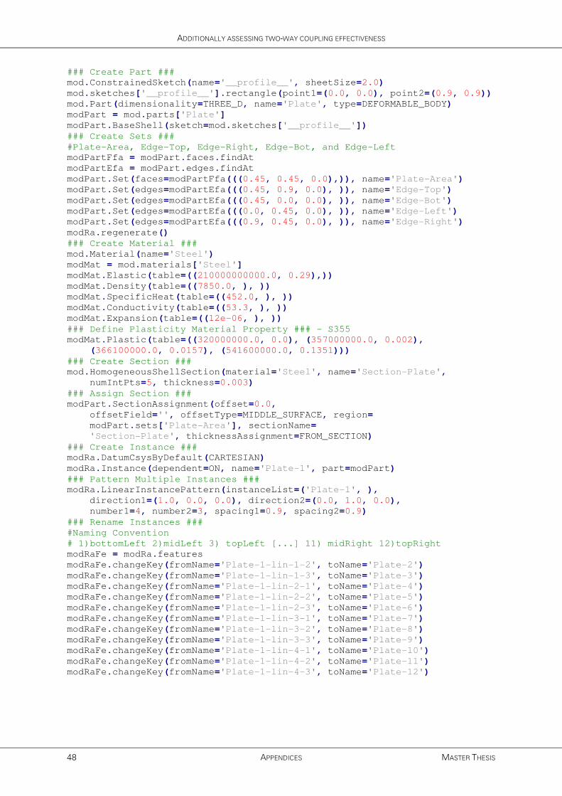
ADDITIONALLY ASSESSING TWO-WAY COUPLING EFFECTIVENESS
48 APPENDICES MASTER THESIS
### Create Part ###
mod.ConstrainedSketch(name='__profile__', sheetSize=2.0)
mod.sketches['__profile__'].rectangle(point1=(0.0, 0.0), point2=(0.9, 0.9))
mod.Part(dimensionality=THREE_D, name='Plate', type=DEFORMABLE_BODY)
modPart = mod.parts['Plate']
modPart.BaseShell(sketch=mod.sketches['__profile__'])
### Create Sets ###
#Plate-Area, Edge-Top, Edge-Right, Edge-Bot, and Edge-Left
modPartFfa = modPart.faces.findAt
modPartEfa = modPart.edges.findAt
modPart.Set(faces=modPartFfa(((0.45, 0.45, 0.0),)), name='Plate-Area')
modPart.Set(edges=modPartEfa(((0.45, 0.9, 0.0), )), name='Edge-Top')
modPart.Set(edges=modPartEfa(((0.45, 0.0, 0.0), )), name='Edge-Bot')
modPart.Set(edges=modPartEfa(((0.0, 0.45, 0.0), )), name='Edge-Left')
modPart.Set(edges=modPartEfa(((0.9, 0.45, 0.0), )), name='Edge-Right')
modRa.regenerate()
### Create Material ###
mod.Material(name='Steel')
modMat = mod.materials['Steel']
modMat.Elastic(table=((210000000000.0, 0.29),))
modMat.Density(table=((7850.0, ), ))
modMat.SpecificHeat(table=((452.0, ), ))
modMat.Conductivity(table=((53.3, ), ))
modMat.Expansion(table=((12e-06, ), ))
### Define Plasticity Material Property ### - S355
modMat.Plastic(table=((320000000.0, 0.0), (357000000.0, 0.002),
(366100000.0, 0.0157), (541600000.0, 0.1351)))
### Create Section ###
mod.HomogeneousShellSection(material='Steel', name='Section-Plate',
numIntPts=5, thickness=0.003)
### Assign Section ###
modPart.SectionAssignment(offset=0.0,
offsetField='', offsetType=MIDDLE_SURFACE, region=
modPart.sets['Plate-Area'], sectionName=
'Section-Plate', thicknessAssignment=FROM_SECTION)
### Create Instance ###
modRa.DatumCsysByDefault(CARTESIAN)
modRa.Instance(dependent=ON, name='Plate-1', part=modPart)
### Pattern Multiple Instances ###
modRa.LinearInstancePattern(instanceList=('Plate-1', ),
direction1=(1.0, 0.0, 0.0), direction2=(0.0, 1.0, 0.0),
number1=4, number2=3, spacing1=0.9, spacing2=0.9)
### Rename Instances ###
#Naming Convention
# 1)bottomLeft 2)midLeft 3) topLeft [...] 11) midRight 12)topRight
modRaFe = modRa.features
modRaFe.changeKey(fromName='Plate-1-lin-1-2', toName='Plate-2')
modRaFe.changeKey(fromName='Plate-1-lin-1-3', toName='Plate-3')
modRaFe.changeKey(fromName='Plate-1-lin-2-1', toName='Plate-4')
modRaFe.changeKey(fromName='Plate-1-lin-2-2', toName='Plate-5')
modRaFe.changeKey(fromName='Plate-1-lin-2-3', toName='Plate-6')
modRaFe.changeKey(fromName='Plate-1-lin-3-1', toName='Plate-7')
modRaFe.changeKey(fromName='Plate-1-lin-3-2', toName='Plate-8')
modRaFe.changeKey(fromName='Plate-1-lin-3-3', toName='Plate-9')
modRaFe.changeKey(fromName='Plate-1-lin-4-1', toName='Plate-10')
modRaFe.changeKey(fromName='Plate-1-lin-4-2', toName='Plate-11')
modRaFe.changeKey(fromName='Plate-1-lin-4-3', toName='Plate-12')

FDS-2-ABAQUS: C++ MANAGED AUTOMATED PYTHON SCRIPTED CFD-FEM COUPLING
J.A. FEENSTRA APPENDICES 49
### Create Step ###
# Step is later modified for current iteration (by upGeomSR).
# Defined here for Field Output Request, and Model Change Interaction.
mod.ImplicitDynamicsStep(name='i0_SR-Step', previous='Initial',
timePeriod=300.0, maxNumInc=10000, application=QUASI_STATIC,
initialInc=0.3, minInc=1e-09, maxInc=25.0, nohaf=OFF, amplitude=RAMP,
alpha=DEFAULT, initialConditions=OFF, nlgeom=ON)
### Request Field Output ###
# Field Output is requested every 5 seconds.
modFOR = mod.fieldOutputRequests['F-Output-1']
modFOR.setValues(timeInterval=5.0, # use this
variables=('S','SSAVG', 'E', 'PE', 'PEEQ', 'U', 'NT', 'TEMP'))
# Field Output is requested for every (Abaqus) increment/iteration.
#modFOR.setValues(frequency=1.0, # or this
# variables=('S','SSAVG', 'E', 'PE', 'PEEQ', 'U', 'NT', 'TEMP'))
### Seed Part ###
modPart.seedEdgeByNumber(constraint=FINER, edges=modPartEfa(
((0.9, 0.7875, 0.0), ), ((0.5625, 0.9, 0.0), ),((0.1125, 0.9, 0.0), ),
((0.0, 0.5625, 0.0), ), ((0.0, 0.1125, 0.0), ),((0.3375, 0.0, 0.0), ),
((0.7875, 0.0, 0.0), ), ((0.9, 0.3375, 0.0), ), ), number=6)
### Mesh Part ###
modPart.generateMesh()
### Set Element Type ###
modPart.setElementType(elemTypes=(ElemType(elemCode=S8R,
elemLibrary=STANDARD), ElemType(elemCode=STRI65,
elemLibrary=STANDARD)), regions=(modPartFfa(((0.6, 0.6, 0.0),),
((0.15, 0.6, 0.0), ), ((0.3, 0.3, 0.0), ), ((0.75, 0.3, 0.0), ), ), ))
### Create BCs ###
# Hinged BCs at top and bottom of every plate
numberOfPlates = 12
for plateCounter in xrange(1,numberOfPlates+1):
thisPlate = 'Plate-' + str(plateCounter)
bcTopName = 'P' + str(plateCounter) + '-BC-Top'
bcBotName = 'P' + str(plateCounter) + '-BC-Bot'
mod.DisplacementBC(createStepName='Initial', name=bcTopName,
region=modRa.instances[thisPlate].sets['Edge-Top'],
u1=SET, u2=SET, u3=SET, ur1=UNSET, ur2=UNSET, ur3=UNSET)
mod.DisplacementBC(createStepName='Initial', name=bcBotName,
region=modRa.instances[thisPlate].sets['Edge-Bot'],
u1=SET, u2=SET, u3=SET, ur1=UNSET, ur2=UNSET, ur3=UNSET)
### Request Restart File ###
mod.steps['i0_SR-Step'].Restart(frequency=0, numberIntervals=1, overlay=ON,
timeMarks=OFF)
### Model Change Interaction ###
mod.ModelChange(name='ModelChange', createStepName='i0_SR-Step',
isRestart=True)
### Define Imperfection ###
# imperfection is removed by upGeomSR for non-initial coupling iterations
mod.keywordBlock.synchVersions(storeNodesAndElements=False)
mod.keywordBlock.insert(115,
'\n*Imperfection, file=i0_buc-Job, step=1\n1, 0.003')
########################## End of SR_basicModel ###########################

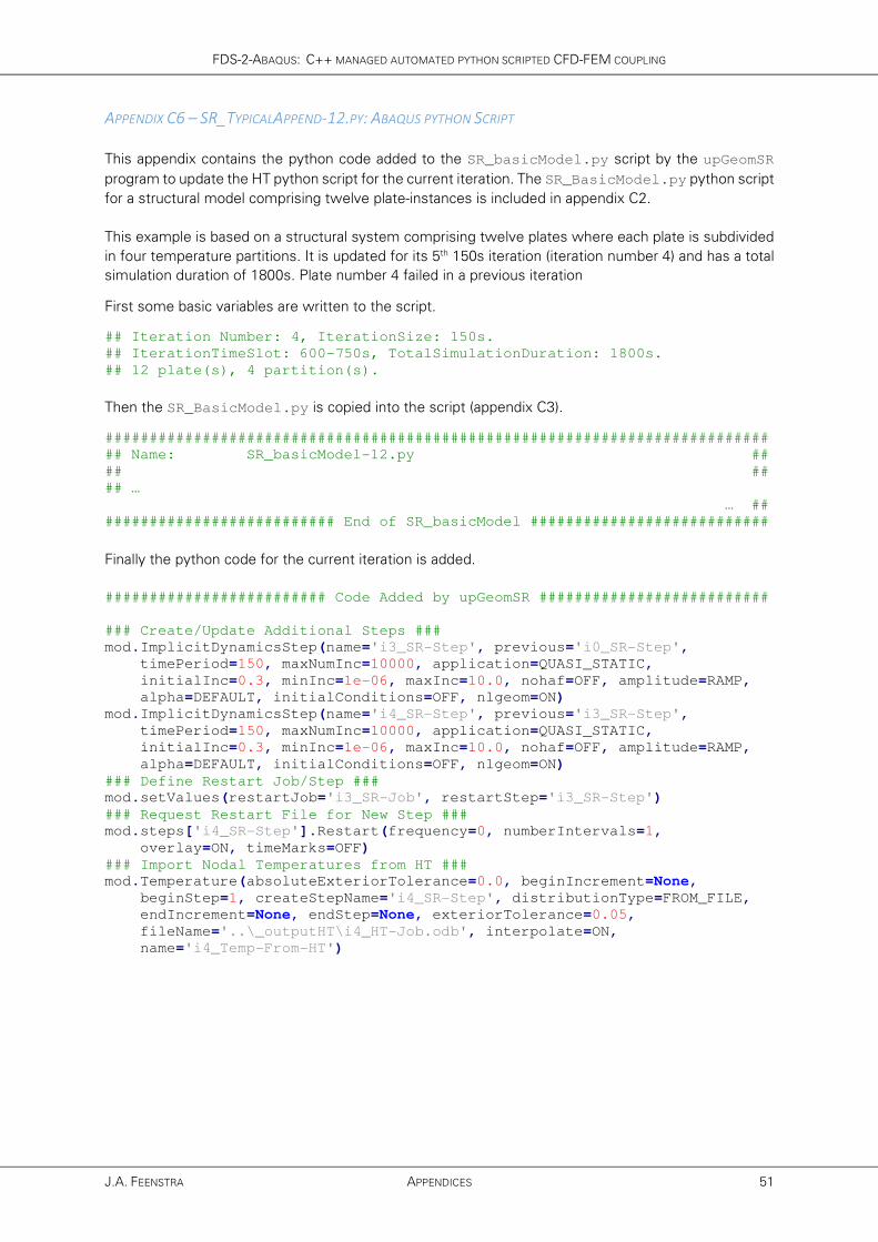
FDS-2-ABAQUS: C++ MANAGED AUTOMATED PYTHON SCRIPTED CFD-FEM COUPLING
J.A. FEENSTRA APPENDICES 51
APPENDIX C6 – SR_TYPICALAPPEND-12.PY: ABAQUS PYTHON SCRIPT
This appendix contains the python code added to the SR_basicModel.py script by the upGeomSR
program to update the HT python script for the current iteration. The SR_BasicModel.py python script
for a structural model comprising twelve plate-instances is included in appendix C2.
This example is based on a structural system comprising twelve plates where each plate is subdivided
in four temperature partitions. It is updated for its 5th 150s iteration (iteration number 4) and has a total
simulation duration of 1800s. Plate number 4 failed in a previous iteration
First some basic variables are written to the script.
## Iteration Number: 4, IterationSize: 150s.
## IterationTimeSlot: 600-750s, TotalSimulationDuration: 1800s.
## 12 plate(s), 4 partition(s).
Then the SR_BasicModel.py is copied into the script (appendix C3).
###########################################################################
## Name: SR_basicModel-12.py ##
## ##
## …
… ##
########################## End of SR_basicModel ###########################
Finally the python code for the current iteration is added.
######################### Code Added by upGeomSR ##########################
### Create/Update Additional Steps ###
mod.ImplicitDynamicsStep(name='i3_SR-Step', previous='i0_SR-Step',
timePeriod=150, maxNumInc=10000, application=QUASI_STATIC,
initialInc=0.3, minInc=1e-06, maxInc=10.0, nohaf=OFF, amplitude=RAMP,
alpha=DEFAULT, initialConditions=OFF, nlgeom=ON)
mod.ImplicitDynamicsStep(name='i4_SR-Step', previous='i3_SR-Step',
timePeriod=150, maxNumInc=10000, application=QUASI_STATIC,
initialInc=0.3, minInc=1e-06, maxInc=10.0, nohaf=OFF, amplitude=RAMP,
alpha=DEFAULT, initialConditions=OFF, nlgeom=ON)
### Define Restart Job/Step ###
mod.setValues(restartJob='i3_SR-Job', restartStep='i3_SR-Step')
### Request Restart File for New Step ###
mod.steps['i4_SR-Step'].Restart(frequency=0, numberIntervals=1,
overlay=ON, timeMarks=OFF)
### Import Nodal Temperatures from HT ###
mod.Temperature(absoluteExteriorTolerance=0.0, beginIncrement=None,
beginStep=1, createStepName='i4_SR-Step', distributionType=FROM_FILE,
endIncrement=None, endStep=None, exteriorTolerance=0.05,
fileName='..\_outputHT\i4_HT-Job.odb', interpolate=ON,
name='i4_Temp-From-HT')
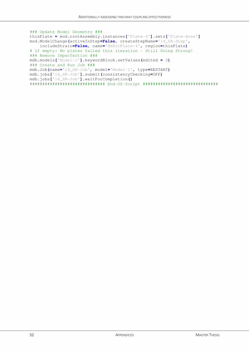
ADDITIONALLY ASSESSING TWO-WAY COUPLING EFFECTIVENESS
52 APPENDICES MASTER THESIS
### Update Model Geometry ###
thisPlate = mod.rootAssembly.instances['Plate-4'].sets['Plate-Area']
mod.ModelChange(activeInStep=False, createStepName='i4_SR-Step',
includeStrain=False, name='deActPlate-4', region=thisPlate)
# If empty: No plates failed this iteration - Still Going Strong!
### Remove Imperfection ###
mdb.models['Model-1'].keywordBlock.setValues(edited = 0)
### Create and Run Job ###
mdb.Job(name='i4_SR-Job', model='Model-1', type=RESTART)
mdb.jobs['i4_SR-Job'].submit(consistencyChecking=OFF)
mdb.jobs['i4_SR-Job'].waitForCompletion()
############################## End-Of-Script ##############################
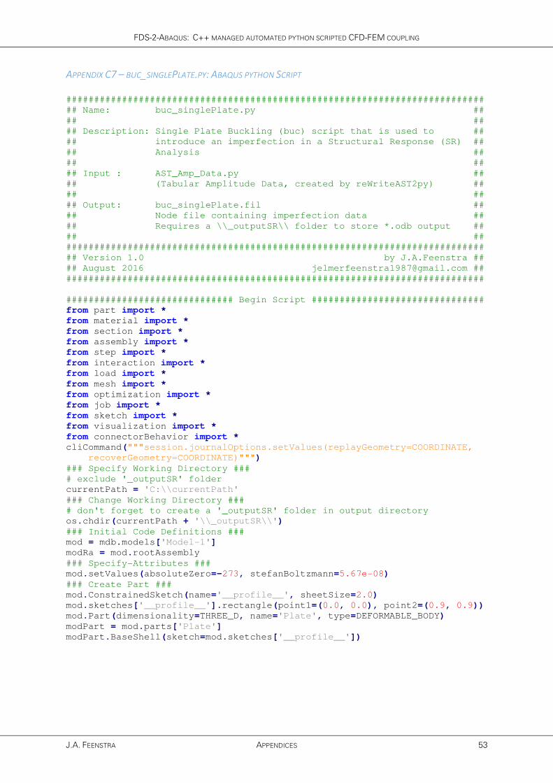
FDS-2-ABAQUS: C++ MANAGED AUTOMATED PYTHON SCRIPTED CFD-FEM COUPLING
J.A. FEENSTRA APPENDICES 53
APPENDIX C7 – BUC_SINGLEPLATE.PY: ABAQUS PYTHON SCRIPT
###########################################################################
## Name: buc_singlePlate.py ##
## ##
## Description: Single Plate Buckling (buc) script that is used to ##
## introduce an imperfection in a Structural Response (SR) ##
## Analysis ##
## ##
## Input : AST_Amp_Data.py ##
## (Tabular Amplitude Data, created by reWriteAST2py) ##
## ##
## Output: buc_singlePlate.fil ##
## Node file containing imperfection data ##
## Requires a \\_outputSR\\ folder to store *.odb output ##
## ##
###########################################################################
## Version 1.0 by J.A.Feenstra ##
## August 2016 [email protected] ##
###########################################################################
############################## Begin Script ###############################
from part import *
from material import *
from section import *
from assembly import *
from step import *
from interaction import *
from load import *
from mesh import *
from optimization import *
from job import *
from sketch import *
from visualization import *
from connectorBehavior import *
cliCommand("""session.journalOptions.setValues(replayGeometry=COORDINATE,
recoverGeometry=COORDINATE)""")
### Specify Working Directory ###
# exclude '_outputSR' folder
currentPath = 'C:\\currentPath'
### Change Working Directory ###
# don't forget to create a '_outputSR' folder in output directory
os.chdir(currentPath + '\\_outputSR\\')
### Initial Code Definitions ###
mod = mdb.models['Model-1']
modRa = mod.rootAssembly
### Specify-Attributes ###
mod.setValues(absoluteZero=-273, stefanBoltzmann=5.67e-08)
### Create Part ###
mod.ConstrainedSketch(name='__profile__', sheetSize=2.0)
mod.sketches['__profile__'].rectangle(point1=(0.0, 0.0), point2=(0.9, 0.9))
mod.Part(dimensionality=THREE_D, name='Plate', type=DEFORMABLE_BODY)
modPart = mod.parts['Plate']
modPart.BaseShell(sketch=mod.sketches['__profile__'])

ADDITIONALLY ASSESSING TWO-WAY COUPLING EFFECTIVENESS
54 APPENDICES MASTER THESIS
### Create Sets ###
#Plate-Area, Edge-Top, Edge-Right, Edge-Bot, and Edge-Left
modPartFfa = modPart.faces.findAt
modPartEfa = modPart.edges.findAt
modPart.Set(faces=modPartFfa(((0.45, 0.45, 0.0),)), name='Plate-Area')
modPart.Set(edges=modPartEfa(((0.45, 0.9, 0.0), )), name='Edge-Top')
modPart.Set(edges=modPartEfa(((0.45, 0.0, 0.0), )), name='Edge-Bot')
modPart.Set(edges=modPartEfa(((0.0, 0.45, 0.0), )), name='Edge-Left')
modPart.Set(edges=modPartEfa(((0.9, 0.45, 0.0), )), name='Edge-Right')
modRa.regenerate()
### Create Material ###
mod.Material(name='Steel')
modMat = mod.materials['Steel']
modMat.Elastic(table=((210000000000.0, 0.29),))
modMat.Density(table=((7850.0, ), ))
modMat.SpecificHeat(table=((452.0, ), ))
modMat.Conductivity(table=((53.3, ), ))
modMat.Expansion(table=((12e-06, ), ))
### Define Plasticity Material Property ### - S355
modMat.Plastic(table=((320000000.0, 0.0), (357000000.0, 0.002),
(366100000.0, 0.0157), (541600000.0, 0.1351)))
### Create Section ###
mod.HomogeneousShellSection(material='Steel', name='Section-Plate',
numIntPts=5, thickness=0.003)
### Assign Section ###
modPart.SectionAssignment(offset=0.0,
offsetField='', offsetType=MIDDLE_SURFACE, region=
modPart.sets['Plate-Area'], sectionName=
'Section-Plate', thicknessAssignment=FROM_SECTION)
### Create Instance ###
modRa.DatumCsysByDefault(CARTESIAN)
modRa.Instance(dependent=ON, name='Plate-1', part=modPart)
### Seed Part ###
modPart.seedEdgeByNumber(constraint=FINER, edges=
modPartEfa(((0.9, 0.7875, 0.0), ), ((0.5625, 0.9, 0.0), ),
((0.1125, 0.9, 0.0), ), ((0.0, 0.5625, 0.0), ), ((0.0, 0.1125, 0.0), ),
((0.3375, 0.0, 0.0), ), ((0.7875, 0.0, 0.0), ),
((0.9, 0.3375, 0.0), ), ), number=6)
### Mesh Part ###
modPart.generateMesh()
### Set Element Type ###
modPart.setElementType(elemTypes=(ElemType(elemCode=S8R,
elemLibrary=STANDARD), ElemType(elemCode=STRI65,
elemLibrary=STANDARD)), regions=(modPartFfa(((0.6, 0.6, 0.0),),
((0.15, 0.6, 0.0), ), ((0.3, 0.3, 0.0), ), ((0.75, 0.3, 0.0), ), ), ))
### Create-Step ###
mod.BuckleStep(description='Buckling Analysis Step',
maxIterations=250, name='i0_buc_step', numEigen=4,
previous='Initial', vectors=8)
### Create-Standardized-Temperature-Field ###
mod.Temperature(name='Buc-Temperature-1', createStepName='i0_buc_step',
magnitudes=(1.0, ),
region=modRa.instances['Plate-1'].sets['Plate-Area'])
### Create BCs ###
mod.DisplacementBC(createStepName='Initial', name='P1-BC-Top',
region=modRa.instances['Plate-1'].sets['Edge-Top'],
u1=SET, u2=SET, u3=SET, ur1=UNSET, ur2=UNSET, ur3=UNSET)
mod.DisplacementBC(createStepName='Initial', name='P1-BC-Bot',
region=modRa.instances['Plate-1'].sets['Edge-Bot'],
u1=SET, u2=SET, u3=SET, ur1=UNSET, ur2=UNSET, ur3=UNSET)
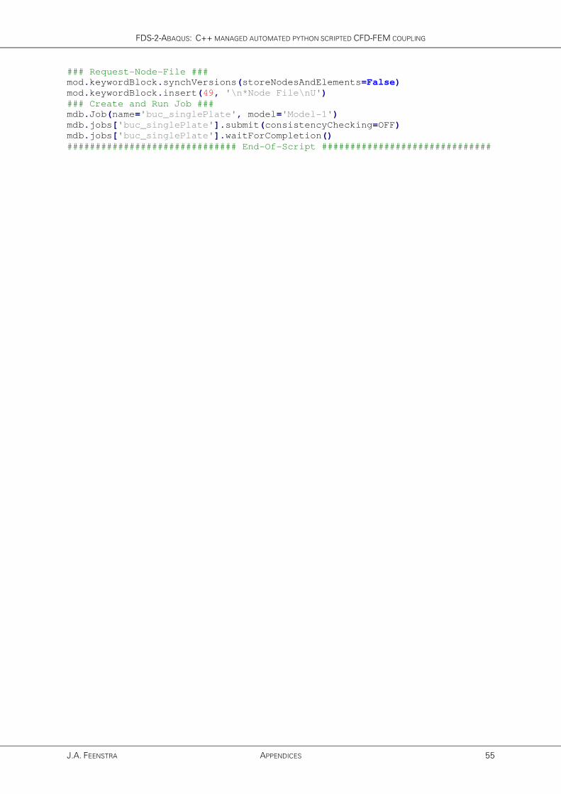
FDS-2-ABAQUS: C++ MANAGED AUTOMATED PYTHON SCRIPTED CFD-FEM COUPLING
J.A. FEENSTRA APPENDICES 55
### Request-Node-File ###
mod.keywordBlock.synchVersions(storeNodesAndElements=False)
mod.keywordBlock.insert(49, '\n*Node File\nU')
### Create and Run Job ###
mdb.Job(name='buc_singlePlate', model='Model-1')
mdb.jobs['buc_singlePlate'].submit(consistencyChecking=OFF)
mdb.jobs['buc_singlePlate'].waitForCompletion()
############################## End-Of-Script ##############################

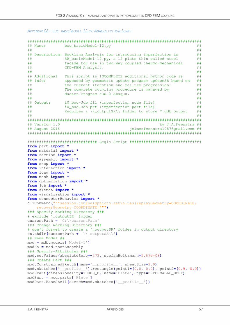
FDS-2-ABAQUS: C++ MANAGED AUTOMATED PYTHON SCRIPTED CFD-FEM COUPLING
J.A. FEENSTRA APPENDICES 57
APPENDIX C8 – BUC_BASICMODEL-12.PY: ABAQUS PYTHON SCRIPT
###########################################################################
## Name: buc_basicModel-12.py ##
## ##
## Description: Buckling Analysis for introducing imperfection in ##
## SR_basicModel-12.py, a 12 plate thin walled steel ##
## facade for use in two-way coupled thermo-mechanical ##
## CFD-FEM Analysis. ##
## ##
## Additional This script is INCOMPLETE additional python code is ##
## Info: appended by geometric update program upGeomSR based on ##
## the current iteration and failure progression. ##
## The complete coupling procedure is managed by ##
## Master Program FDS-2-Abaqus. ##
## ##
## Output: i0_buc-Job.fil (imperfection node file) ##
## i0_buc-Job.prt (imperfection part file) ##
## Requires a \\_outputSR\\ folder to store *.odb output ##
## ##
###########################################################################
## Version 1.0 by J.A.Feenstra ##
## August 2016 [email protected] ##
###########################################################################
############################## Begin Script ###############################
from part import *
from material import *
from section import *
from assembly import *
from step import *
from interaction import *
from load import *
from mesh import *
from optimization import *
from job import *
from sketch import *
from visualization import *
from connectorBehavior import *
cliCommand("""session.journalOptions.setValues(replayGeometry=COORDINATE,
recoverGeometry=COORDINATE)""")
### Specify Working Directory ###
# exclude '_outputSR' folder
currentPath = 'C:\\currentPath'
### Change Working Directory ###
# don't forget to create a '_outputSR' folder in output directory
os.chdir(currentPath + '\\_outputSR\\')
## Name Model ##
mod = mdb.models['Model-1']
modRa = mod.rootAssembly
### Specify-Attributes ###
mod.setValues(absoluteZero=-273, stefanBoltzmann=5.67e-08)
### Create Part ###
mod.ConstrainedSketch(name='__profile__', sheetSize=2.0)
mod.sketches['__profile__'].rectangle(point1=(0.0, 0.0), point2=(0.9, 0.9))
mod.Part(dimensionality=THREE_D, name='Plate', type=DEFORMABLE_BODY)
modPart = mod.parts['Plate']
modPart.BaseShell(sketch=mod.sketches['__profile__'])
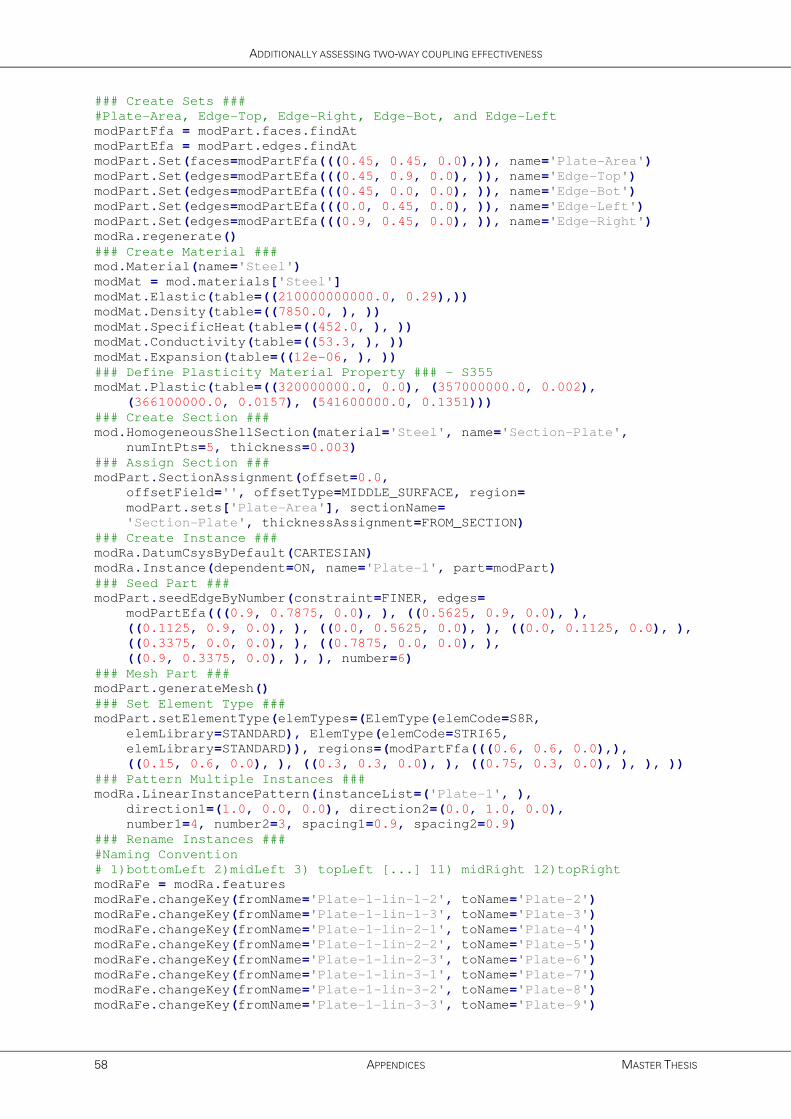
ADDITIONALLY ASSESSING TWO-WAY COUPLING EFFECTIVENESS
58 APPENDICES MASTER THESIS
### Create Sets ###
#Plate-Area, Edge-Top, Edge-Right, Edge-Bot, and Edge-Left
modPartFfa = modPart.faces.findAt
modPartEfa = modPart.edges.findAt
modPart.Set(faces=modPartFfa(((0.45, 0.45, 0.0),)), name='Plate-Area')
modPart.Set(edges=modPartEfa(((0.45, 0.9, 0.0), )), name='Edge-Top')
modPart.Set(edges=modPartEfa(((0.45, 0.0, 0.0), )), name='Edge-Bot')
modPart.Set(edges=modPartEfa(((0.0, 0.45, 0.0), )), name='Edge-Left')
modPart.Set(edges=modPartEfa(((0.9, 0.45, 0.0), )), name='Edge-Right')
modRa.regenerate()
### Create Material ###
mod.Material(name='Steel')
modMat = mod.materials['Steel']
modMat.Elastic(table=((210000000000.0, 0.29),))
modMat.Density(table=((7850.0, ), ))
modMat.SpecificHeat(table=((452.0, ), ))
modMat.Conductivity(table=((53.3, ), ))
modMat.Expansion(table=((12e-06, ), ))
### Define Plasticity Material Property ### - S355
modMat.Plastic(table=((320000000.0, 0.0), (357000000.0, 0.002),
(366100000.0, 0.0157), (541600000.0, 0.1351)))
### Create Section ###
mod.HomogeneousShellSection(material='Steel', name='Section-Plate',
numIntPts=5, thickness=0.003)
### Assign Section ###
modPart.SectionAssignment(offset=0.0,
offsetField='', offsetType=MIDDLE_SURFACE, region=
modPart.sets['Plate-Area'], sectionName=
'Section-Plate', thicknessAssignment=FROM_SECTION)
### Create Instance ###
modRa.DatumCsysByDefault(CARTESIAN)
modRa.Instance(dependent=ON, name='Plate-1', part=modPart)
### Seed Part ###
modPart.seedEdgeByNumber(constraint=FINER, edges=
modPartEfa(((0.9, 0.7875, 0.0), ), ((0.5625, 0.9, 0.0), ),
((0.1125, 0.9, 0.0), ), ((0.0, 0.5625, 0.0), ), ((0.0, 0.1125, 0.0), ),
((0.3375, 0.0, 0.0), ), ((0.7875, 0.0, 0.0), ),
((0.9, 0.3375, 0.0), ), ), number=6)
### Mesh Part ###
modPart.generateMesh()
### Set Element Type ###
modPart.setElementType(elemTypes=(ElemType(elemCode=S8R,
elemLibrary=STANDARD), ElemType(elemCode=STRI65,
elemLibrary=STANDARD)), regions=(modPartFfa(((0.6, 0.6, 0.0),),
((0.15, 0.6, 0.0), ), ((0.3, 0.3, 0.0), ), ((0.75, 0.3, 0.0), ), ), ))
### Pattern Multiple Instances ###
modRa.LinearInstancePattern(instanceList=('Plate-1', ),
direction1=(1.0, 0.0, 0.0), direction2=(0.0, 1.0, 0.0),
number1=4, number2=3, spacing1=0.9, spacing2=0.9)
### Rename Instances ###
#Naming Convention
# 1)bottomLeft 2)midLeft 3) topLeft [...] 11) midRight 12)topRight
modRaFe = modRa.features
modRaFe.changeKey(fromName='Plate-1-lin-1-2', toName='Plate-2')
modRaFe.changeKey(fromName='Plate-1-lin-1-3', toName='Plate-3')
modRaFe.changeKey(fromName='Plate-1-lin-2-1', toName='Plate-4')
modRaFe.changeKey(fromName='Plate-1-lin-2-2', toName='Plate-5')
modRaFe.changeKey(fromName='Plate-1-lin-2-3', toName='Plate-6')
modRaFe.changeKey(fromName='Plate-1-lin-3-1', toName='Plate-7')
modRaFe.changeKey(fromName='Plate-1-lin-3-2', toName='Plate-8')
modRaFe.changeKey(fromName='Plate-1-lin-3-3', toName='Plate-9')

FDS-2-ABAQUS: C++ MANAGED AUTOMATED PYTHON SCRIPTED CFD-FEM COUPLING
J.A. FEENSTRA APPENDICES 59
modRaFe.changeKey(fromName='Plate-1-lin-4-1', toName='Plate-10')
modRaFe.changeKey(fromName='Plate-1-lin-4-2', toName='Plate-11')
modRaFe.changeKey(fromName='Plate-1-lin-4-3', toName='Plate-12')
## Create Node Sets ##
n = modPart.nodes
nodesLeft = n[7:8]+n[14:15]+n[21:22]+n[28:29]+n[35:36]+n[52:53]+n[70:71]\
+n[83:84]+n[96:97]+n[109:110]+n[122:123]
modPart.Set(nodes=nodesLeft, name='Edge-Left-Node')
nodesRight = n[13:14]+n[20:21]+n[27:28]+n[34:35]+n[41:42]+n[66:67]\
+n[79:80]+n[92:93]+n[105:106]+n[118:119]+n[131:132]
modPart.Set(nodes=nodesRight, name='Edge-Right-Node')
### Tie Instances ###
# Convention: Lower plateNumber = Master
## Plate 1 Ties ##
mod.Tie(name='Tie_P1-P2',
master=modRa.instances['Plate-1'].sets['Edge-Top'],
slave=modRa.instances['Plate-2'].sets['Edge-Bot'],
positionToleranceMethod=COMPUTED, adjust=ON)
mod.Tie(name='Tie_P1-P4',
master=modRa.instances['Plate-1'].sets['Edge-Right-Node'],
slave=modRa.instances['Plate-4'].sets['Edge-Left-Node'],
positionToleranceMethod=COMPUTED, adjust=ON)
## Plate 2 Ties ##
mod.Tie(name='Tie_P2-P3',
master=modRa.instances['Plate-2'].sets['Edge-Top'],
slave=modRa.instances['Plate-3'].sets['Edge-Bot'],
positionToleranceMethod=COMPUTED, adjust=ON)
mod.Tie(name='Tie_P2-P5',
master=modRa.instances['Plate-2'].sets['Edge-Right-Node'],
slave=modRa.instances['Plate-5'].sets['Edge-Left-Node'],
positionToleranceMethod=COMPUTED, adjust=ON)
## Plate 3 Ties ##
mod.Tie(name='Tie_P3-P6',
master=modRa.instances['Plate-3'].sets['Edge-Right-Node'],
slave=modRa.instances['Plate-6'].sets['Edge-Left-Node'],
positionToleranceMethod=COMPUTED, adjust=ON)
## Plate 4 Ties ##
mod.Tie(name='Tie_P4-P5',
master=modRa.instances['Plate-4'].sets['Edge-Top'],
slave=modRa.instances['Plate-5'].sets['Edge-Bot'],
positionToleranceMethod=COMPUTED, adjust=ON)
mod.Tie(name='Tie_P4-P7',
master=modRa.instances['Plate-4'].sets['Edge-Right-Node'],
slave=modRa.instances['Plate-7'].sets['Edge-Left-Node'],
positionToleranceMethod=COMPUTED, adjust=ON)
## Plate 5 Ties ##
mod.Tie(name='Tie_P5-P6',
master=modRa.instances['Plate-5'].sets['Edge-Top'],
slave=modRa.instances['Plate-6'].sets['Edge-Bot'],
positionToleranceMethod=COMPUTED, adjust=ON)
mod.Tie(name='Tie_P5-P8',
master=modRa.instances['Plate-5'].sets['Edge-Right-Node'],
slave=modRa.instances['Plate-8'].sets['Edge-Left-Node'],
positionToleranceMethod=COMPUTED, adjust=ON)
## Plate 6 Ties ##
mod.Tie(name='Tie_P6-P9',
master=modRa.instances['Plate-6'].sets['Edge-Right-Node'],
slave=modRa.instances['Plate-9'].sets['Edge-Left-Node'],
positionToleranceMethod=COMPUTED, adjust=ON)

ADDITIONALLY ASSESSING TWO-WAY COUPLING EFFECTIVENESS
60 APPENDICES MASTER THESIS
## Plate 7 Ties ##
mod.Tie(name='Tie_P7-P8',
master=modRa.instances['Plate-7'].sets['Edge-Top'],
slave=modRa.instances['Plate-8'].sets['Edge-Bot'],
positionToleranceMethod=COMPUTED, adjust=ON)
mod.Tie(name='Tie_P7-P10',
master=modRa.instances['Plate-7'].sets['Edge-Right-Node'],
slave=modRa.instances['Plate-10'].sets['Edge-Left-Node'],
positionToleranceMethod=COMPUTED, adjust=ON)
## Plate 8 Ties ##
mod.Tie(name='Tie_P8-P9',
master=modRa.instances['Plate-8'].sets['Edge-Top'],
slave=modRa.instances['Plate-9'].sets['Edge-Bot'],
positionToleranceMethod=COMPUTED, adjust=ON)
mod.Tie(name='Tie_P8-P11',
master=modRa.instances['Plate-8'].sets['Edge-Right-Node'],
slave=modRa.instances['Plate-11'].sets['Edge-Left-Node'],
positionToleranceMethod=COMPUTED, adjust=ON)
## Plate 9 Ties ##
mod.Tie(name='Tie_P9-P12',
master=modRa.instances['Plate-9'].sets['Edge-Right-Node'],
slave=modRa.instances['Plate-12'].sets['Edge-Left-Node'],
positionToleranceMethod=COMPUTED, adjust=ON)
## Plate 10 Ties ##
mod.Tie(name='Tie_P10-P11',
master=modRa.instances['Plate-10'].sets['Edge-Top'],
slave=modRa.instances['Plate-11'].sets['Edge-Bot'],
positionToleranceMethod=COMPUTED, adjust=ON)
## Plate 11 Ties ##
mod.Tie(name='Tie_P11-P12',
master=modRa.instances['Plate-11'].sets['Edge-Top'],
slave=modRa.instances['Plate-12'].sets['Edge-Bot'],
positionToleranceMethod=COMPUTED, adjust=ON)
### Create-Step ###
mod.BuckleStep(description='Buckling Analysis Step',
maxIterations=250, name='i0_buc_step', numEigen=4,
previous='Initial', vectors=8)
### Create-Standardized-Temperature-Field ###
mod.Temperature(name='Buc-Temperature-1', createStepName='i0_buc_step',
magnitudes=(1.0, ),
region=modRa.instances['Plate-1'].sets['Plate-Area'])
mod.Temperature(name='Buc-Temperature-2', createStepName='i0_buc_step',
magnitudes=(1.0, ),
region=modRa.instances['Plate-2'].sets['Plate-Area'])
mod.Temperature(name='Buc-Temperature-3', createStepName='i0_buc_step',
magnitudes=(1.0, ),
region=modRa.instances['Plate-3'].sets['Plate-Area'])
mod.Temperature(name='Buc-Temperature-4', createStepName='i0_buc_step',
magnitudes=(1.0, ),
region=modRa.instances['Plate-4'].sets['Plate-Area'])
mod.Temperature(name='Buc-Temperature-5', createStepName='i0_buc_step',
magnitudes=(1.0, ),
region=modRa.instances['Plate-5'].sets['Plate-Area'])
mod.Temperature(name='Buc-Temperature-6', createStepName='i0_buc_step',
magnitudes=(1.0, ),
region=modRa.instances['Plate-6'].sets['Plate-Area'])
mod.Temperature(name='Buc-Temperature-7', createStepName='i0_buc_step',
magnitudes=(1.0, ),
region=modRa.instances['Plate-7'].sets['Plate-Area'])
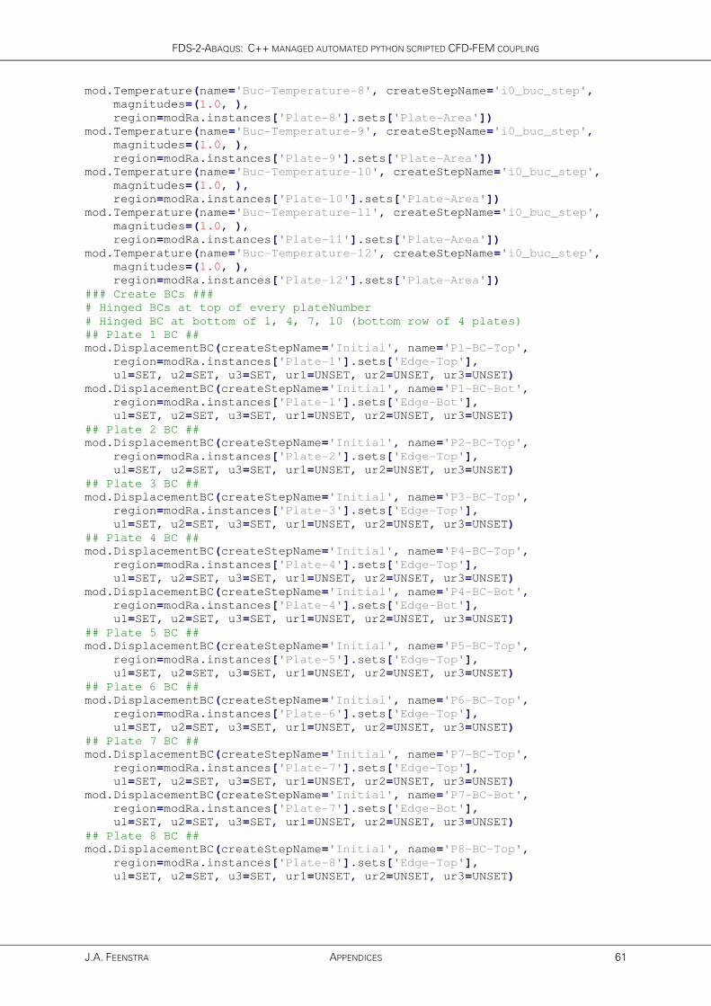
FDS-2-ABAQUS: C++ MANAGED AUTOMATED PYTHON SCRIPTED CFD-FEM COUPLING
J.A. FEENSTRA APPENDICES 61
mod.Temperature(name='Buc-Temperature-8', createStepName='i0_buc_step',
magnitudes=(1.0, ),
region=modRa.instances['Plate-8'].sets['Plate-Area'])
mod.Temperature(name='Buc-Temperature-9', createStepName='i0_buc_step',
magnitudes=(1.0, ),
region=modRa.instances['Plate-9'].sets['Plate-Area'])
mod.Temperature(name='Buc-Temperature-10', createStepName='i0_buc_step',
magnitudes=(1.0, ),
region=modRa.instances['Plate-10'].sets['Plate-Area'])
mod.Temperature(name='Buc-Temperature-11', createStepName='i0_buc_step',
magnitudes=(1.0, ),
region=modRa.instances['Plate-11'].sets['Plate-Area'])
mod.Temperature(name='Buc-Temperature-12', createStepName='i0_buc_step',
magnitudes=(1.0, ),
region=modRa.instances['Plate-12'].sets['Plate-Area'])
### Create BCs ###
# Hinged BCs at top of every plateNumber
# Hinged BC at bottom of 1, 4, 7, 10 (bottom row of 4 plates)
## Plate 1 BC ##
mod.DisplacementBC(createStepName='Initial', name='P1-BC-Top',
region=modRa.instances['Plate-1'].sets['Edge-Top'],
u1=SET, u2=SET, u3=SET, ur1=UNSET, ur2=UNSET, ur3=UNSET)
mod.DisplacementBC(createStepName='Initial', name='P1-BC-Bot',
region=modRa.instances['Plate-1'].sets['Edge-Bot'],
u1=SET, u2=SET, u3=SET, ur1=UNSET, ur2=UNSET, ur3=UNSET)
## Plate 2 BC ##
mod.DisplacementBC(createStepName='Initial', name='P2-BC-Top',
region=modRa.instances['Plate-2'].sets['Edge-Top'],
u1=SET, u2=SET, u3=SET, ur1=UNSET, ur2=UNSET, ur3=UNSET)
## Plate 3 BC ##
mod.DisplacementBC(createStepName='Initial', name='P3-BC-Top',
region=modRa.instances['Plate-3'].sets['Edge-Top'],
u1=SET, u2=SET, u3=SET, ur1=UNSET, ur2=UNSET, ur3=UNSET)
## Plate 4 BC ##
mod.DisplacementBC(createStepName='Initial', name='P4-BC-Top',
region=modRa.instances['Plate-4'].sets['Edge-Top'],
u1=SET, u2=SET, u3=SET, ur1=UNSET, ur2=UNSET, ur3=UNSET)
mod.DisplacementBC(createStepName='Initial', name='P4-BC-Bot',
region=modRa.instances['Plate-4'].sets['Edge-Bot'],
u1=SET, u2=SET, u3=SET, ur1=UNSET, ur2=UNSET, ur3=UNSET)
## Plate 5 BC ##
mod.DisplacementBC(createStepName='Initial', name='P5-BC-Top',
region=modRa.instances['Plate-5'].sets['Edge-Top'],
u1=SET, u2=SET, u3=SET, ur1=UNSET, ur2=UNSET, ur3=UNSET)
## Plate 6 BC ##
mod.DisplacementBC(createStepName='Initial', name='P6-BC-Top',
region=modRa.instances['Plate-6'].sets['Edge-Top'],
u1=SET, u2=SET, u3=SET, ur1=UNSET, ur2=UNSET, ur3=UNSET)
## Plate 7 BC ##
mod.DisplacementBC(createStepName='Initial', name='P7-BC-Top',
region=modRa.instances['Plate-7'].sets['Edge-Top'],
u1=SET, u2=SET, u3=SET, ur1=UNSET, ur2=UNSET, ur3=UNSET)
mod.DisplacementBC(createStepName='Initial', name='P7-BC-Bot',
region=modRa.instances['Plate-7'].sets['Edge-Bot'],
u1=SET, u2=SET, u3=SET, ur1=UNSET, ur2=UNSET, ur3=UNSET)
## Plate 8 BC ##
mod.DisplacementBC(createStepName='Initial', name='P8-BC-Top',
region=modRa.instances['Plate-8'].sets['Edge-Top'],
u1=SET, u2=SET, u3=SET, ur1=UNSET, ur2=UNSET, ur3=UNSET)

ADDITIONALLY ASSESSING TWO-WAY COUPLING EFFECTIVENESS
62 APPENDICES MASTER THESIS
## Plate 9 BC ##
mod.DisplacementBC(createStepName='Initial', name='P9-BC-Top',
region=modRa.instances['Plate-9'].sets['Edge-Top'],
u1=SET, u2=SET, u3=SET, ur1=UNSET, ur2=UNSET, ur3=UNSET)
## Plate 10 BC ##
mod.DisplacementBC(createStepName='Initial', name='P10-BC-Top',
region=modRa.instances['Plate-10'].sets['Edge-Top'],
u1=SET, u2=SET, u3=SET, ur1=UNSET, ur2=UNSET, ur3=UNSET)
mod.DisplacementBC(createStepName='Initial', name='P10-BC-Bot',
region=modRa.instances['Plate-10'].sets['Edge-Bot'],
u1=SET, u2=SET, u3=SET, ur1=UNSET, ur2=UNSET, ur3=UNSET)
## Plate 11 BC ##
mod.DisplacementBC(createStepName='Initial', name='P11-BC-Top',
region=modRa.instances['Plate-11'].sets['Edge-Top'],
u1=SET, u2=SET, u3=SET, ur1=UNSET, ur2=UNSET, ur3=UNSET)
## Plate 12 BC ##
mod.DisplacementBC(createStepName='Initial', name='P12-BC-Top',
region=modRa.instances['Plate-12'].sets['Edge-Top'],
u1=SET, u2=SET, u3=SET, ur1=UNSET, ur2=UNSET, ur3=UNSET)
### Request-Node-File ###
mod.keywordBlock.synchVersions(storeNodesAndElements=False)
mod.keywordBlock.insert(244, '\n*Node File\nU')
### Create Job ###
mdb.Job(name='i0_buc-Job', model='Model-1')
### Run Job ###
mdb.jobs['i0_buc-Job'].submit(consistencyChecking=OFF)
mdb.jobs['i0_buc-Job'].waitForCompletion()
############################## End-Of-Script ##############################
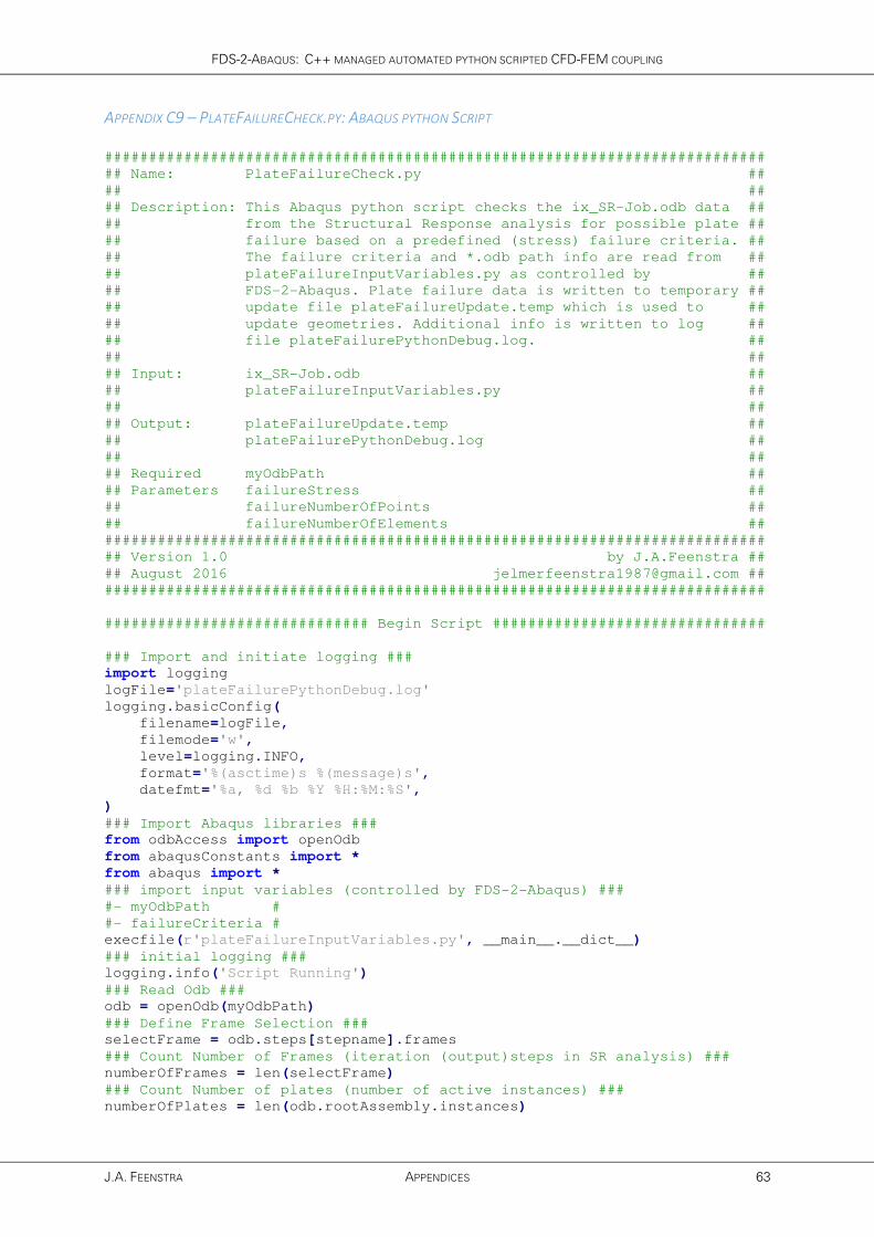
FDS-2-ABAQUS: C++ MANAGED AUTOMATED PYTHON SCRIPTED CFD-FEM COUPLING
J.A. FEENSTRA APPENDICES 63
APPENDIX C9 – PLATEFAILURECHECK.PY: ABAQUS PYTHON SCRIPT
###########################################################################
## Name: PlateFailureCheck.py ##
## ##
## Description: This Abaqus python script checks the ix_SR-Job.odb data ##
## from the Structural Response analysis for possible plate ##
## failure based on a predefined (stress) failure criteria. ##
## The failure criteria and *.odb path info are read from ##
## plateFailureInputVariables.py as controlled by ##
## FDS-2-Abaqus. Plate failure data is written to temporary ##
## update file plateFailureUpdate.temp which is used to ##
## update geometries. Additional info is written to log ##
## file plateFailurePythonDebug.log. ##
## ##
## Input: ix_SR-Job.odb ##
## plateFailureInputVariables.py ##
## ##
## Output: plateFailureUpdate.temp ##
## plateFailurePythonDebug.log ##
## ##
## Required myOdbPath ##
## Parameters failureStress ##
## failureNumberOfPoints ##
## failureNumberOfElements ##
###########################################################################
## Version 1.0 by J.A.Feenstra ##
## August 2016 [email protected] ##
###########################################################################
############################## Begin Script ###############################
### Import and initiate logging ###
import logging
logFile='plateFailurePythonDebug.log'
logging.basicConfig(
filename=logFile,
filemode='w',
level=logging.INFO,
format='%(asctime)s %(message)s',
datefmt='%a, %d %b %Y %H:%M:%S',
)
### Import Abaqus libraries ###
from odbAccess import openOdb
from abaqusConstants import *
from abaqus import *
### import input variables (controlled by FDS-2-Abaqus) ###
#- myOdbPath #
#- failureCriteria #
execfile(r'plateFailureInputVariables.py', __main__.__dict__)
### initial logging ###
logging.info('Script Running')
### Read Odb ###
odb = openOdb(myOdbPath)
### Define Frame Selection ###
selectFrame = odb.steps[stepname].frames
### Count Number of Frames (iteration (output)steps in SR analysis) ###
numberOfFrames = len(selectFrame)
### Count Number of plates (number of active instances) ###
numberOfPlates = len(odb.rootAssembly.instances)
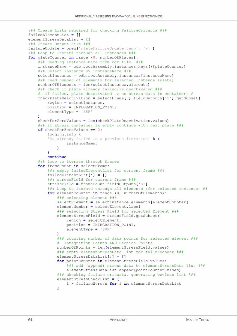
ADDITIONALLY ASSESSING TWO-WAY COUPLING EFFECTIVENESS
64 APPENDICES MASTER THESIS
### Create Lists required for checking FailureCriteria ###
failedElementList = []
elementStressDataList = []
### Create Output File ###
failureUpdate = open('plateFailureUpdate.temp', 'w' )
### Loop to iterate through all instances ###
for plateCounter in range (0, numberOfPlates):
### Reading Instance-name from odb file. ###
instanceName = odb.rootAssembly.instances.keys()[plateCounter]
### Select instance by instanceName ###
selectInstance = odb.rootAssembly.instances[instanceName]
### read number of Elements for selected Instance (plate)
numberOfElements = len(selectInstance.elements)
### check if plate already failed/is deactivated ###
#- if failed, plate deactivated -> no stress data in container) #
checkPlateDeactivation = selectFrame[0].fieldOutputs['S'].getSubset(
region = selectInstance,
position = INTEGRATION_POINT,
elementType = 'S8R'
)
checkForZeroValues = len(checkPlateDeactivation.values)
### if stress container is empty continue with next plate ###
if checkForZeroValues == 0:
logging.info (
'%s already failed in a previous iteration' % (
instanceName,
)
)
continue
### loop to iterate through frames
for frameCount in selectFrame:
### empty failedElementList for current frame ###
failedElementList[:] = []
### stressField for current frame ###
stressField = frameCount.fieldOutputs['S']
### Loop to iterate through all elements (for selected instance) ##
for elementCounter in range (0, numberOfElements):
### selecting element ###
selectElement = selectInstance.elements[elementCounter]
elementNumber = selectElement.label
### selecting Stress Field for selected Element ###
elementStressField = stressField.getSubset(
region = selectElement,
position = INTEGRATION_POINT,
elementType = 'S8R'
)
### counting number of data points for selected element ###
#- Integration Points AND Section Points
numberOfPoints = len(elementStressField.values)
### empty elementStressData list for failurecheck ###
elementStressDataList[:] = []
for pointCounter in elementStressField.values:
### add (append) stress data to elementStressData list ###
elementStressDataList.append(pointCounter.mises)
### checking failure criteria, generating boolean list ###
elementStressCheckList = [
i > failureStress for i in elementStressDataList
]
FDS-2-ABAQUS: C++ MANAGED AUTOMATED PYTHON SCRIPTED CFD-FEM COUPLING
J.A. FEENSTRA APPENDICES 65
### counting number of 'True' (=failed points) ###
#- in boolean list elementStressCheck
elementNumberOfFailedPoints = elementStressCheckList.\
count(True)
### statement checking if element is considered failed ###
#- based on failureCriteria
if elementNumberOfFailedPoints >= failureNumberOfPoints:
failedElementList.append(True)
else:
failedElementList.append(False)
### counting number of 'True' (=failed elements) ###
#- in boolean list failedElementList
numberOfFailedElements = failedElementList.count(True)
### check failure criteria (elements) ###
if numberOfFailedElements >= failureNumberOfElements:
### write plateFailure data to update-file ###
failureUpdate.write('%s %d\n' % (
instanceName,
frameCount.frameValue
)
)
### write plateFailure to logfile (debugging) ###
logging.info (
'%s failed at t=%d seconds since %d elements failed' % (
instanceName,
frameCount.frameValue,
numberOfFailedElements
)
)
### Break 'frameCount for loop' when plate failed ###
break
### write info on non-failed plates to logfile (debugging) ###
if numberOfFailedElements < failureNumberOfElements:
logging.info ('%s did not fail, still going strong'
% (instanceName)
)
### Finalize and close plateFailureUpdate.temp ###
failureUpdate.write('Done')
failureUpdate.close()
### Finalize log file ###
logging.info ('Completed')
### output completed message to console ###
print 'Completed, see plateFailurePythonDebug.log for details'
############################ End-of-Script ############################ ############################ PlateFailureCheck ############################

FDS-2-ABAQUS: C++ MANAGED AUTOMATED PYTHON SCRIPTED CFD-FEM COUPLING
J.A. FEENSTRA APPENDICES 67
APPENDIX D1 – FDS-2-ABAQUS: C++ SOURCE CODE
///////////////////////////////////////////////////////////////////////////
// Name: FDS-2-Abaqus //
// //
// Description: This program manages the two-way coupling of a //
// CFD Fire Dynamic Simulator (FDS) fire simulation and //
// a sequential coupled FE Abaqus Heat Transfer (HT) and //
// Structural Response (SR) analysis. In its current state //
// FDS-2-Abaqus is limited to analyzing structures //
// consisting of multiple plate-instances using a stress- //
// based failure criteria. The number of plates, //
// temperature partitions, simulation duration, iteration //
// size, and failure criteria can be varied freely (as //
// long as required FDS and Abaqus basic model setups //
// are supplied). Basically the programs iterates through //
// various one way coupled CFD-FEM analyses. After every //
// iteration the program checks plate failure based on //
// user-defined stress failure criteria. If failure occurs //
// the plates are removed from the models (FDS and Abaqus) //
// for the next iteration. The overview of plate failure //
// and failure time points is written to _plateFailure.log. //
// //
// Input: plateFailureUpdate.temp //
// //
// Output: _plateFailure.log //
// _iterationCounter.temp //
// _platePartitionCounter.temp //
// _runIterationTemp.bat //
// plateFailureInputVariables.py //
// //
// Required numberOfPlates (user console input) //
// Parameters: numberOfPartitions (user console input) //
// totalSimulationDuration (user console input) //
// iterationSize (user console input) //
// failureStress (user console input) //
// failureNumberOfPoints (user console input) //
// failureNumberOfElements (user console input) //
// failedPlateNumber //
// failureTimePoint //
///////////////////////////////////////////////////////////////////////////
// Version 1.0 by J.A.Feenstra //
// August 2016 [email protected] //
///////////////////////////////////////////////////////////////////////////
/////////////////////////////// Begin Code ////////////////////////////////
// Import Libraries //
#include <iostream>
#include <string>
#include <fstream>
#include <cstdlib>
#include <sstream>
#include <stdlib.h>
#include <windows.h>
#include <iomanip>
#include <regex>
#include <limits>
// Import boost Libraries //
#include <boost/lexical_cast.hpp>

ADDITIONALLY ASSESSING TWO-WAY COUPLING EFFECTIVENESS
68 APPENDICES MASTER THESIS
// Define String Parameters //
// output filename to (temporary) store iteration data //
// used in: upGeomFDS, upGeomHT, upGeomSR,
std::string counterFileName = "_iterationCounter.temp";
// output filename to (temporary) store plate/partition info //
// used in: reWriteAST2py, upGeomHT, upGeomSR
std::string platePartitionFileName = "_platePartitionInfo.temp";
// filename for (temporary) batch file containing program //
// sequence for single iteration loop //
std::string batchScriptFileName = "_runIterationTemp.bat";
// output filename for log managing plate failure //
// used in: upGeomFDS, upGeomHT, upGeomSR //
std::string plateFailureFileName = "_plateFailure.log";
// input filename containing possible plate failure //
// for current iteration (managed by PlateFailureCheck.py) //
std::string updatePlateFailureFileName = "plateFailureUpdate.temp";
// output filename for storing input variables for checking failure //
// used in: PlateFailureCheck.py //
std::string plateFailureInputVariablesFileName =
"plateFailureInputVariables.py";
// inputString to store line from updatePlateFailureFilename //
std::string inputString;
// filename strings for verification if required files exist //
std::string upGeomFDS = "upGeomFDS.exe";
std::string fdsBasicSetup = "FDS_BasicSetup.fds";
std::string reWriteAST2py = "reWriteAST2py.exe";
std::string upGeomHT = "upGeomHT.exe";
std::string htBasicModel= "HT_basicModel.py";
std::string upGeomSR = "upGeomSR.exe";
std::string srBasicModel = "SR_basicModel.py";
std::string plateFailureCheck = "PlateFailureCheck.py";
std::string bucImperfectionFil = "_outputSR\\i0_buc-Job.fil";
std::string bucImperfectionPrt = "_outputSR\\i0_buc-Job.prt";
std::string exists = "Exists!";
std::string missing = "Missing!";
// Define Integer Parameters //
// numberOfPlates, user input see function request_basic_variables //
int numberOfPlates(1);
// numberOfPartitions, user input see function request_basic_variables //
int numberOfPartitions(1);
// totalSimulationDuration, user input see func. request_basic_variables //
int totalSimulationDuration(50);
// iterationSize, user input see function request_basic_variables //
int iterationSize(10);
// iterationCounter starts at 0 (zeroth iteration) //
int iterationCounter(0); // do not edit //
// arrayCounter to be used in for loops iterating through //
// array managing _plateFailure.log info //
int arrayCounter(0);
// Plate/Instance number of failed plate //
// read from plateFailureFileName //
int failedPlateNumber(0);
// failure time point for plate 'failedPlateNumber' //
// read from plateFailureFileName //
int failureTimePoint(0);
// Counter managing number of failed plates //
int numberOfFailedPlates(0);
FDS-2-ABAQUS: C++ MANAGED AUTOMATED PYTHON SCRIPTED CFD-FEM COUPLING
J.A. FEENSTRA APPENDICES 69
// failureStress, user input, see function update_failure_criteria //
int failureStress(355); // [N/mm^2]
// number of SP/IP that should satisfy failure criteria //
// before element is considered failed. //
// user input, see function update_failure criteria //
int failureNumberOfPoints(4);
// number of elements that should satisfy failure criteria //
// before plate is considered failed. //
// user input, see function update_failure criteria //
int failureNumberOfElements(12);
// Define char variables //
// choice char for selecting/storing yes/no questions //
char choice;
// function requesting input to continue //
// 'pause' function //
void press_enter_to_continue()
{
std::cin.clear();
std::cout << "Press ENTER to continue...";
std::cin.ignore(std::numeric_limits<std::streamsize>::max(), '\n');
}
// function to print banner logo to console //
void print_banner_to_console()
{
// ASCII Title-Art //
std::cout << '\n';
std::cout << " ) "
<< " __ __ __ __ "
<< " ) " << '\n';
std::cout << " ) \\ "
<< "|_ | \\(_ __ _) __ /\\ |_ _ _ _ "
<< " ) \\ " << '\n';
std::cout << " / ) ( "
<< "| |__/__) /__ /--\\|_)(_|(_||_|_) "
<< " / ) ( " << '\n';
std::cout << " \\(_)/ "
<< " | "
<< " \\(_)/ " << '\n';
std::cout << '\n';
// Version and Author Info //
std::cout << "Version 1.0 "
<< "by J.A.Feenstra" << '\n';
std::cout << "August 2016 "
<< "[email protected]" << '\n';
std::cout << '\n';
}
ADDITIONALLY ASSESSING TWO-WAY COUPLING EFFECTIVENESS
70 APPENDICES MASTER THESIS
// function to print banner and introductory info to console //
// NOTE: maximum characters on line = 60 //
void welcome_world()
{
print_banner_to_console();
std::cout << "[ [ [Description] ] ]" << '\n'
<< "FDS-2-Abaqus manages the two-way coupling of a CFD Fire " << '\n'
<< "Dynamic Simulator (FDS) fire simulation and a sequential "<< '\n'
<< "coupled FE Abaqus Heat Transfer (HT) and Structural " << '\n'
<< "Response (SR) analysis." << '\n' << '\n';
std::cout << "[ [ [Checking Required Files] ] ]" << '\n'
<< "FDS-2-Abaqus will now check if all required files are " << '\n'
<< "supplied. If any are MISSING verify file(name)s and paths!" <<'\n';
press_enter_to_continue();
std::cout << '\n';
}
// function to check if file exists or are missing //
std::string check_file_existence(const std::string& name)
{
if (FILE *file = fopen(name.c_str(), "r")){
fclose(file);
return exists;
}
else{
return missing;
}
}
void verify_existence_required_files()
{
std::cout << "[ [ [Required Programs] ] ]" << '\n'
<< "reWriteAST2py.exe "
<< check_file_existence(reWriteAST2py) << '\n'
<< "upGeomFDS.exe "
<< check_file_existence(upGeomFDS) << '\n'
<< "upGeomHT.exe "
<< check_file_existence(upGeomHT) << '\n'
<< "upGeomSR.exe "
<< check_file_existence(upGeomSR) << '\n';
std::cout << "[ [ [Required Scripts] ] ]" << '\n'
<< "FDS_BasicSetup.fds "
<< check_file_existence(fdsBasicSetup) << '\n'
<< "HT_basicModel.py "
<< check_file_existence(htBasicModel) << '\n'
<< "SR_basicModel.py "
<< check_file_existence(srBasicModel) << '\n'
<< "PlateFailureCheck.py "
<< check_file_existence(plateFailureCheck) << '\n';
std::cout << "[ [ [Required Buckling File] ] ]" << '\n'
<< "i0_buc-Job.fil "
<< check_file_existence(bucImperfectionFil) << '\n'
<< "i0_buc-Job.prt "
<< check_file_existence(bucImperfectionPrt) << '\n'
<< "(in \\_outputSR\\ folder)" << '\n';
std::cout << '\n';
}
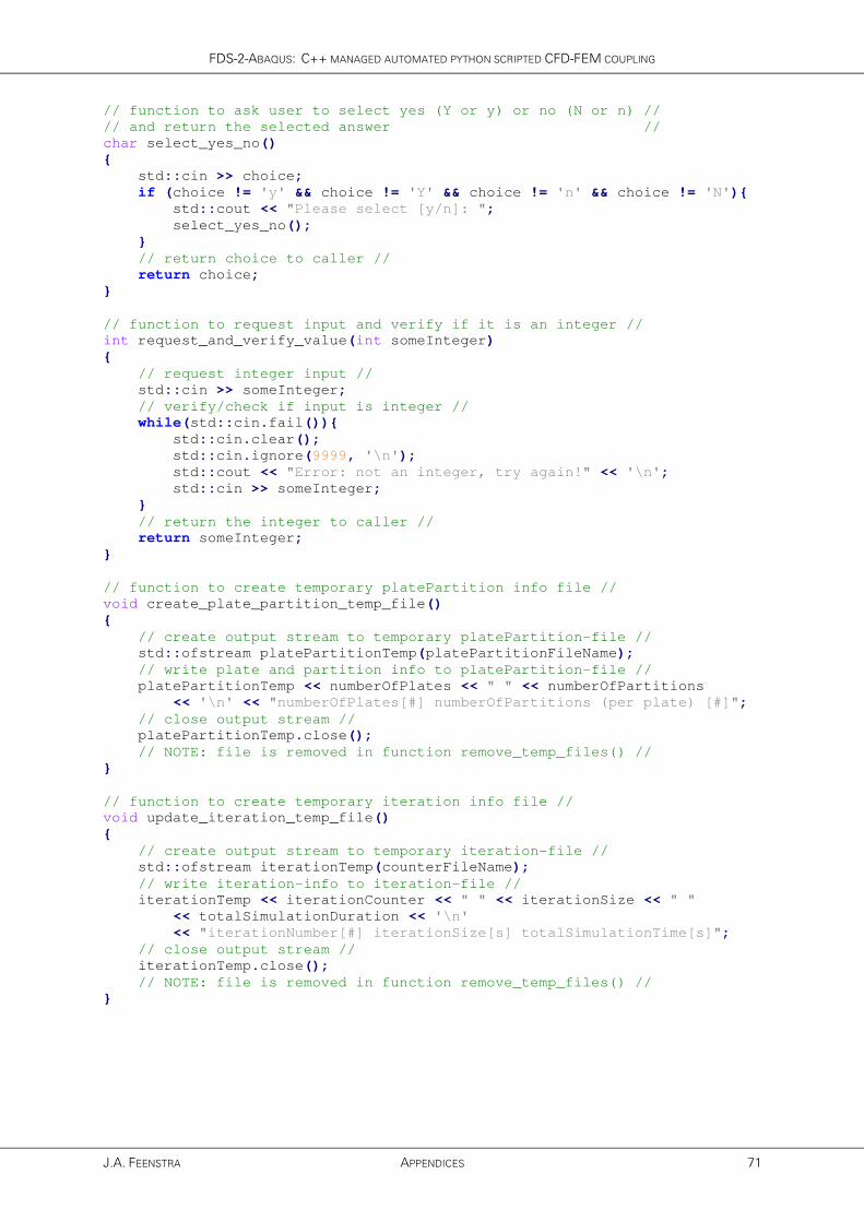
FDS-2-ABAQUS: C++ MANAGED AUTOMATED PYTHON SCRIPTED CFD-FEM COUPLING
J.A. FEENSTRA APPENDICES 71
// function to ask user to select yes (Y or y) or no (N or n) //
// and return the selected answer //
char select_yes_no()
{
std::cin >> choice;
if (choice != 'y' && choice != 'Y' && choice != 'n' && choice != 'N'){
std::cout << "Please select [y/n]: ";
select_yes_no();
}
// return choice to caller //
return choice;
}
// function to request input and verify if it is an integer //
int request_and_verify_value(int someInteger)
{
// request integer input //
std::cin >> someInteger;
// verify/check if input is integer //
while(std::cin.fail()){
std::cin.clear();
std::cin.ignore(9999, '\n');
std::cout << "Error: not an integer, try again!" << '\n';
std::cin >> someInteger;
}
// return the integer to caller //
return someInteger;
}
// function to create temporary platePartition info file //
void create_plate_partition_temp_file()
{
// create output stream to temporary platePartition-file //
std::ofstream platePartitionTemp(platePartitionFileName);
// write plate and partition info to platePartition-file //
platePartitionTemp << numberOfPlates << " " << numberOfPartitions
<< '\n' << "numberOfPlates[#] numberOfPartitions (per plate) [#]";
// close output stream //
platePartitionTemp.close();
// NOTE: file is removed in function remove_temp_files() //
}
// function to create temporary iteration info file //
void update_iteration_temp_file()
{
// create output stream to temporary iteration-file //
std::ofstream iterationTemp(counterFileName);
// write iteration-info to iteration-file //
iterationTemp << iterationCounter << " " << iterationSize << " "
<< totalSimulationDuration << '\n'
<< "iterationNumber[#] iterationSize[s] totalSimulationTime[s]";
// close output stream //
iterationTemp.close();
// NOTE: file is removed in function remove_temp_files() //
}
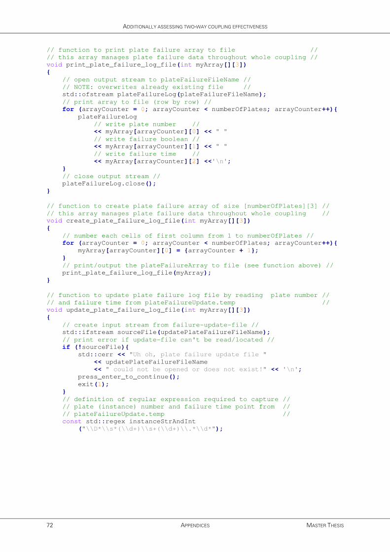
ADDITIONALLY ASSESSING TWO-WAY COUPLING EFFECTIVENESS
72 APPENDICES MASTER THESIS
// function to print plate failure array to file //
// this array manages plate failure data throughout whole coupling //
void print_plate_failure_log_file(int myArray[][3])
{
// open output stream to plateFailureFileName //
// NOTE: overwrites already existing file //
std::ofstream plateFailureLog(plateFailureFileName);
// print array to file (row by row) //
for (arrayCounter = 0; arrayCounter < numberOfPlates; arrayCounter++){
plateFailureLog
// write plate number //
<< myArray[arrayCounter][0] << " "
// write failure boolean //
<< myArray[arrayCounter][1] << " "
// write failure time //
<< myArray[arrayCounter][2] <<'\n';
}
// close output stream //
plateFailureLog.close();
}
// function to create plate failure array of size [numberOfPlates][3] //
// this array manages plate failure data throughout whole coupling //
void create_plate_failure_log_file(int myArray[][3])
{
// number each cells of first column from 1 to numberOfPlates //
for (arrayCounter = 0; arrayCounter < numberOfPlates; arrayCounter++){
myArray[arrayCounter][0] = {arrayCounter + 1};
}
// print/output the plateFailureArray to file (see function above) //
print_plate_failure_log_file(myArray);
}
// function to update plate failure log file by reading plate number //
// and failure time from plateFailureUpdate.temp //
void update_plate_failure_log_file(int myArray[][3])
{
// create input stream from failure-update-file //
std::ifstream sourceFile(updatePlateFailureFileName);
// print error if update-file can't be read/located //
if (!sourceFile){
std::cerr << "Uh oh, plate failure update file "
<< updatePlateFailureFileName
<< " could not be opened or does not exist!" << '\n';
press_enter_to_continue();
exit(1);
}
// definition of regular expression required to capture //
// plate (instance) number and failure time point from //
// plateFailureUpdate.temp //
const std::regex instanceStrAndInt
("\\D*\\s*(\\d+)\\s+(\\d+)\\.*\\d*");

FDS-2-ABAQUS: C++ MANAGED AUTOMATED PYTHON SCRIPTED CFD-FEM COUPLING
J.A. FEENSTRA APPENDICES 73
// while end of file isn't reached do this //
while(!sourceFile.eof()){
// get line and put the line in the string inputString //
getline(sourceFile, inputString);
// break (end) while loop if getline reads Done //
if (inputString == "Done"){
std::cout << "Failure Check Completed!" << '\n' << '\n';
break;
}
// if input string matches regular expression (it should) //
else if(std::regex_match(inputString, instanceStrAndInt)){
// match (string) results into stringMatch //
std::smatch stringMatch;
if (std::regex_search(inputString, stringMatch,
instanceStrAndInt)){
// cast obtained 'strings' as integers //
failedPlateNumber =
boost::lexical_cast<int>(stringMatch[1]);
failureTimePoint =
boost::lexical_cast<int>(stringMatch[2]) +
(iterationCounter * iterationSize);
// output plateFailure to console //
std::cout << "! ! ! F A I L U R E ! ! !" << '\n'
<< "Plate " << failedPlateNumber
<< " Failed @ " << failureTimePoint << " seconds"
<< '\n';
// print error if an already failed plate fails again //
if (myArray[failedPlateNumber - 1][1] == 1){
std::cerr << "Error! An already Failed Plate, "
<<"Failed Again. This should not happen!" << '\n'
<<"Please check scripts/models!";
exit(1);
}
// update plateFailureArray for this itteration //
// write failure boolean and failureTimePoint //
myArray[failedPlateNumber - 1][1] = 1;
myArray[failedPlateNumber - 1][2] = failureTimePoint;
numberOfFailedPlates++;
// continue with while loop //
continue;
}
}
}
// close input stream //
sourceFile.close();
// print/output the plateFailureArray to file //
print_plate_failure_log_file(myArray);
}
// function to request basic values from user and some verification //
void request_basic_variables()
{
std::cout << "[ [ [ Request Input Variables] ] ]" << '\n'
<< "FDS-2-Abaqus will now request some basic input variables." << '\n'
<< "Make sure the numberOfPlates and numberOfPartitions agree " << '\n'
<< "with the variables defined in the basicModel input files " << '\n'
<< "and scripts." << '\n' << '\n';
std::cout << "[ [ [Basic Model Info] ] ]" << '\n';
// request numberOfPlates //
std::cout << "Please enter the number of plates [#]: ";
numberOfPlates = request_and_verify_value(numberOfPlates);

ADDITIONALLY ASSESSING TWO-WAY COUPLING EFFECTIVENESS
74 APPENDICES MASTER THESIS
// request numberOfTemperaturePartitions //
std::cout << "Please enter the number of temperature " << '\n'
<< "partitions for each plate [#]: ";
numberOfPartitions = request_and_verify_value(numberOfPartitions);
// request totalSimulationDuration and iterationSize and verify //
// if totalsimulationDuration > iterationSize //
do{
if (iterationSize > totalSimulationDuration){
std::cout << "Error! iteration size larger than total "
<< "simulation duration, try again!" << '\n';
}
// request totalSimulationDuration //
std::cout << "Please enter the total simulation duration [s]: ";
totalSimulationDuration =
request_and_verify_value(totalSimulationDuration);
// request iterationSize //
std::cout << "Please enter the iteration size [s]: ";
iterationSize = request_and_verify_value(iterationSize);
}
while (iterationSize > totalSimulationDuration);
// list selected values //
std::cout << '\n' << "You selected the values listed below:" << '\n'
<< "Number of Plates = " << numberOfPlates << " plate(s)" << '\n'
<< "Number of Temperature Partitions (per plate) = "
<< numberOfPartitions << " partition(s)" << '\n'
<< "Total Simulation Duration = " << totalSimulationDuration
<< " seconds" << '\n'
<< "Iteration Size = " << iterationSize << " seconds" << '\n'
<< '\n';
// ask user if selected input is correct //
std::cout << "are these values correct [y/n]? ";
select_yes_no();
// if no -> request new input ('restart function') //
if (choice == 'n' || choice == 'N'){
std::cout << '\n';
request_basic_variables();
}
// if yes -> continue //
else if (choice == 'y' || choice == 'Y'){
std::cout << '\n';
// nothing really happens here //
}
// this should never happen, only y,Y,n, or N can be returned //
else{
std::cerr << "This should never happen only [y/n] is returned";
press_enter_to_continue();
exit(1);
}
}
// function to list 'standard' failure parameters and the possibility //
// to change these parameters //
void update_failure_criteria()
{
// list standard values //
std::cout << "[ [ [Failure Criteria] ] ]" << '\n'
<< "Failure Stress = " << failureStress << " N/mm^2" << '\n'
<< "Number of Failed Points required to consider Element "
<< "as failed: " << failureNumberOfPoints << '\n'
<< "Number of Failed Elements required to consider Plate "
<< "as failed: " << failureNumberOfElements << '\n';

FDS-2-ABAQUS: C++ MANAGED AUTOMATED PYTHON SCRIPTED CFD-FEM COUPLING
J.A. FEENSTRA APPENDICES 75
// ask user if standard input is correct //
std::cout << '\n' << "are these values correct [y/n]? ";
select_yes_no();
// if no ask user for new failure input //
if (choice == 'n' || choice == 'N'){
std::cout << '\n';
std::cout << "[ [ [Failure Criteria] ] ]" << '\n';
// request failureStress value //
std::cout << "Please enter the Failure Stress [N/mm^2]: ";
failureStress = request_and_verify_value(failureStress);
// request failureNumberOfPoints //
std::cout << "Please enter the number of Failed Points required "
<< '\n' << "to consider Element as failed [#]: ";
failureNumberOfPoints =
request_and_verify_value(failureNumberOfPoints);
std::cout << "Please enter the number Failed Elements required "
<< '\n' << "to consider Plate as failed [#]: ";
// request failureNumberOfElements //
failureNumberOfElements =
request_and_verify_value(failureNumberOfElements);
std::cout << '\n' << "You selected the values listed below: "
<< '\n';
// write values to plateFailureInputVariables.py //
update_failure_criteria();
}
// if yes -> continue //
else if (choice == 'y' || choice == 'Y'){
std::cout << std::endl;
// final check before running simulation //
std::cout << "[ [ [ Final Check ] ] ]" << '\n'
<< "FDS-2-Abaqus is now ready to begin the coupling procedure!"
<< '\n'
<< "Select YES [y] to start the coupling simulation, select "
<< '\n'
<< "NO [n] to re-enter input variables." << '\n' << '\n'
<< "Start Simulation?: ";
// selecting NO allows user to re-enter input variables //
select_yes_no();
if (choice == 'n' || choice == 'N'){
std::cout << '\n';
request_basic_variables();
update_failure_criteria();
}
}
// this should never happen, only y,Y,n, or N can be returned //
else{
std::cerr << "This should never happen only [y/n] is returned";
press_enter_to_continue();
exit(1);
}
}
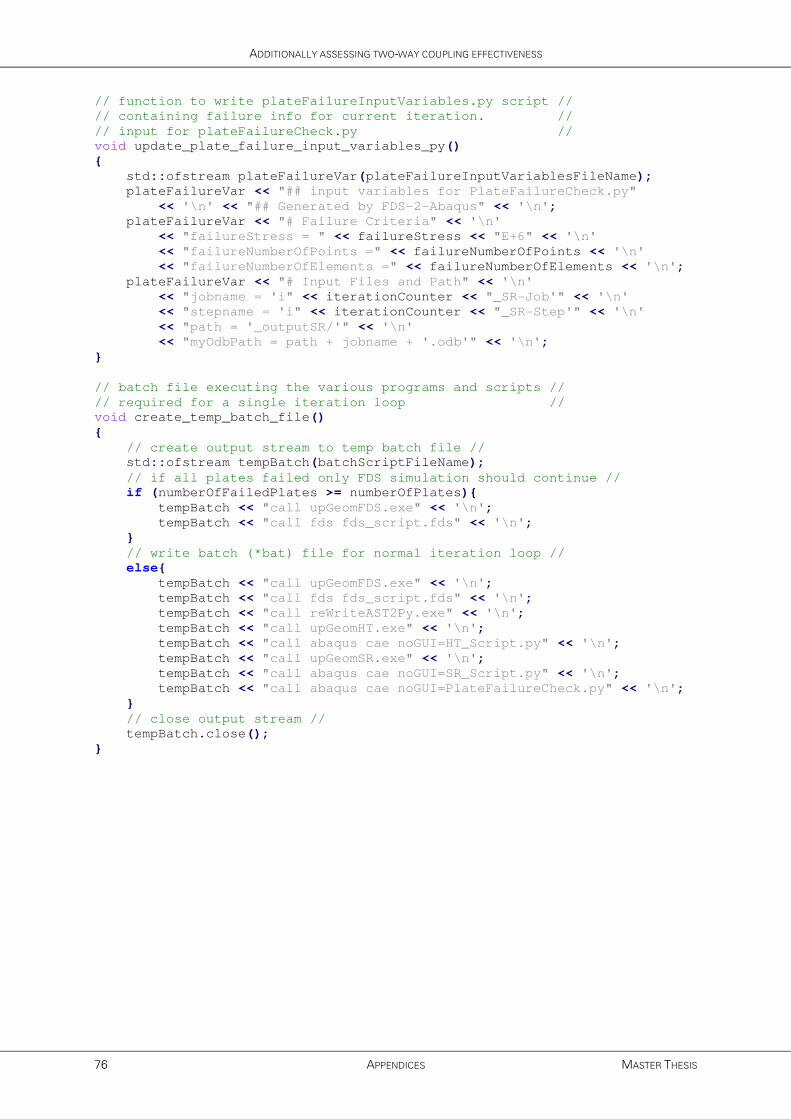
ADDITIONALLY ASSESSING TWO-WAY COUPLING EFFECTIVENESS
76 APPENDICES MASTER THESIS
// function to write plateFailureInputVariables.py script //
// containing failure info for current iteration. //
// input for plateFailureCheck.py //
void update_plate_failure_input_variables_py()
{
std::ofstream plateFailureVar(plateFailureInputVariablesFileName);
plateFailureVar << "## input variables for PlateFailureCheck.py"
<< '\n' << "## Generated by FDS-2-Abaqus" << '\n';
plateFailureVar << "# Failure Criteria" << '\n'
<< "failureStress = " << failureStress << "E+6" << '\n'
<< "failureNumberOfPoints =" << failureNumberOfPoints << '\n'
<< "failureNumberOfElements =" << failureNumberOfElements << '\n';
plateFailureVar << "# Input Files and Path" << '\n'
<< "jobname = 'i" << iterationCounter << "_SR-Job'" << '\n'
<< "stepname = 'i" << iterationCounter << "_SR-Step'" << '\n'
<< "path = '_outputSR/'" << '\n'
<< "myOdbPath = path + jobname + '.odb'" << '\n';
}
// batch file executing the various programs and scripts //
// required for a single iteration loop //
void create_temp_batch_file()
{
// create output stream to temp batch file //
std::ofstream tempBatch(batchScriptFileName);
// if all plates failed only FDS simulation should continue //
if (numberOfFailedPlates >= numberOfPlates){
tempBatch << "call upGeomFDS.exe" << '\n';
tempBatch << "call fds fds_script.fds" << '\n';
}
// write batch (*bat) file for normal iteration loop //
else{
tempBatch << "call upGeomFDS.exe" << '\n';
tempBatch << "call fds fds_script.fds" << '\n';
tempBatch << "call reWriteAST2Py.exe" << '\n';
tempBatch << "call upGeomHT.exe" << '\n';
tempBatch << "call abaqus cae noGUI=HT_Script.py" << '\n';
tempBatch << "call upGeomSR.exe" << '\n';
tempBatch << "call abaqus cae noGUI=SR_Script.py" << '\n';
tempBatch << "call abaqus cae noGUI=PlateFailureCheck.py" << '\n';
}
// close output stream //
tempBatch.close();
}
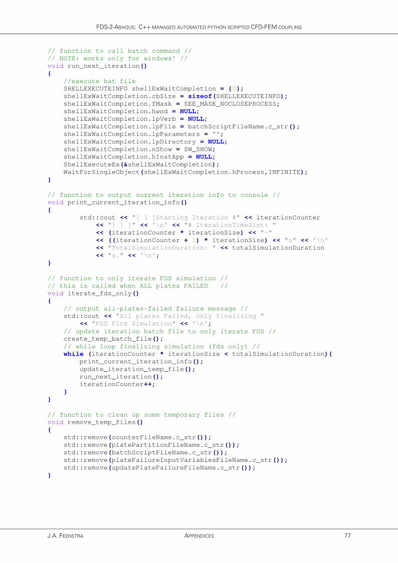
FDS-2-ABAQUS: C++ MANAGED AUTOMATED PYTHON SCRIPTED CFD-FEM COUPLING
J.A. FEENSTRA APPENDICES 77
// function to call batch command //
// NOTE: works only for windows! //
void run_next_iteration()
{
//execute bat file
SHELLEXECUTEINFO shellExWaitCompletion = {0};
shellExWaitCompletion.cbSize = sizeof(SHELLEXECUTEINFO);
shellExWaitCompletion.fMask = SEE_MASK_NOCLOSEPROCESS;
shellExWaitCompletion.hwnd = NULL;
shellExWaitCompletion.lpVerb = NULL;
shellExWaitCompletion.lpFile = batchScriptFileName.c_str();
shellExWaitCompletion.lpParameters = "";
shellExWaitCompletion.lpDirectory = NULL;
shellExWaitCompletion.nShow = SW_SHOW;
shellExWaitCompletion.hInstApp = NULL;
ShellExecuteEx(&shellExWaitCompletion);
WaitForSingleObject(shellExWaitCompletion.hProcess,INFINITE);
}
// function to output current iteration info to console //
void print_current_iteration_info()
{
std::cout << "[ [ [Starting Iteration #" << iterationCounter
<< "] ] ]" << '\n' << "# IterationTimeSlot: "
<< (iterationCounter * iterationSize) << "-"
<< ((iterationCounter + 1) * iterationSize) << "s" << '\n'
<< "TotalSimulationDuration: " << totalSimulationDuration
<< "s." << '\n';
}
// function to only iterate FDS simulation //
// this is called when ALL plates FAILED //
void iterate_fds_only()
{
// output all-plates-failed failure message //
std::cout << "All plates Failed, only finalizing "
<< "FDS Fire Simulation" << '\n';
// update iteration batch file to only iterate FDS //
create_temp_batch_file();
// while loop finalizing simulation (fds only) //
while (iterationCounter * iterationSize < totalSimulationDuration){
print_current_iteration_info();
update_iteration_temp_file();
run_next_iteration();
iterationCounter++;
}
}
// function to clean up some temporary files //
void remove_temp_files()
{
std::remove(counterFileName.c_str());
std::remove(platePartitionFileName.c_str());
std::remove(batchScriptFileName.c_str());
std::remove(plateFailureInputVariablesFileName.c_str());
std::remove(updatePlateFailureFileName.c_str());
}

ADDITIONALLY ASSESSING TWO-WAY COUPLING EFFECTIVENESS
78 APPENDICES MASTER THESIS
// function to output starting info to console //
void print_start_coupling_analysis()
{
std::cout << "[ [ [ S T A R T I N G C O U P L I N G "
<< "A N A L Y S I S ] ] ]" << '\n' << '\n';
}
// function to output completion info to console //
void print_completion_info_and_failureArray(int myArray[][3])
{
std::cout << "[ [ [ C O U P L I N G A N A L Y S I S "
<< "C O M P L E T E D ] ] ]" << '\n';
print_banner_to_console();
// Simulation Overview/Summary //
std::cout << "[ [ [Overview of Failed Plates] ] ] " << '\n'
<< "Number of Plates: " << numberOfPlates << '\n'
<< "Number of Failed Plates: " << numberOfFailedPlates << '\n';
for (arrayCounter = 0; arrayCounter < numberOfPlates; arrayCounter++){
if (myArray[arrayCounter][1] == 1){
std::cout << "Plate " << myArray[arrayCounter][0]
<< " Failed @ " << myArray[arrayCounter][2]
<< " seconds" << '\n';
}
}
std::cout << '\n'
<< "NOTE: Always check FDS (*.out) and Abaqus (*.msg)" << '\n'
<< " files for possible errors!" << '\n';
std::cout << '\n' << "[ [ [ Thank You For Using FDS-2-Abaqus ] ] ]"
<< '\n';
press_enter_to_continue();
press_enter_to_continue();
}
int main()
{
// welcome and introductory info //
welcome_world();
// check if required files exist (in path) //
verify_existence_required_files();
// request #plate, #partition, sim. duration, and iteration size //
request_basic_variables();
// check and/or request failure criteria //
update_failure_criteria();
// create temporary platePartition file //
create_plate_partition_temp_file();
// define plateFailureArray //
// this is defined here since numberOfPlates is required //
int plateFailureArray[numberOfPlates][3] = {0};
// create plate failure log file //
create_plate_failure_log_file(plateFailureArray);
// create batch file executing the various programs and scripts //
// for a single iteration loop //
create_temp_batch_file();
// Just a banner (time stamps should be included)
print_start_coupling_analysis();

FDS-2-ABAQUS: C++ MANAGED AUTOMATED PYTHON SCRIPTED CFD-FEM COUPLING
J.A. FEENSTRA APPENDICES 79
// while loop iterating through all steps in //
// the fully coupled simulation //
while(iterationCounter * iterationSize < totalSimulationDuration){
if (numberOfFailedPlates >= numberOfPlates){
iterate_fds_only();
break;
}
// output current iteration info to console //
print_current_iteration_info();
// update current iteration to temporary file //
update_iteration_temp_file();
// update input variables for plateFailureCheck.py //
// plateFailureCheck.py checks plate failure //
update_plate_failure_input_variables_py();
// run batch file executing the various programs and scripts //
run_next_iteration();
// update and print _plateFailure.log //
update_plate_failure_log_file(plateFailureArray);
// next iteration
iterationCounter++;
}
// output completion info to console //
print_completion_info_and_failureArray(plateFailureArray);
// clean up some temporary files //
//remove_temp_files();
return 0;
}
////////////////////////////// End of Code //////////////////////////////
////////////////////////////// FDS-2-Abaqus //////////////////////////////

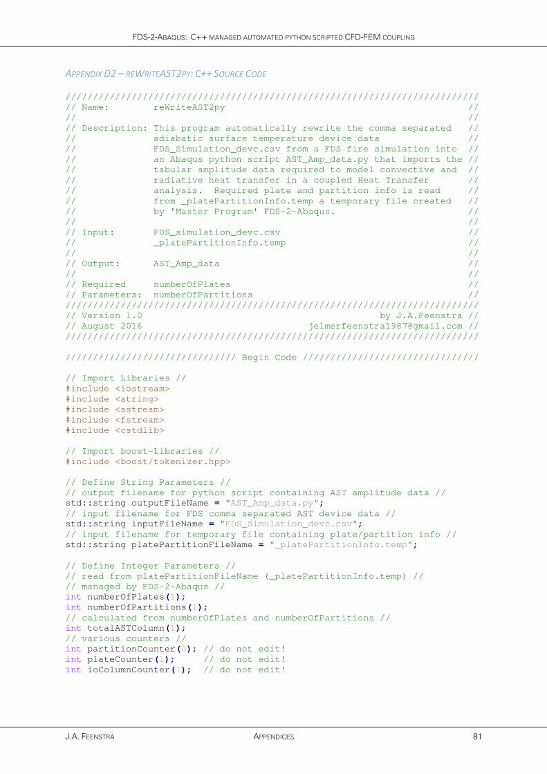
FDS-2-ABAQUS: C++ MANAGED AUTOMATED PYTHON SCRIPTED CFD-FEM COUPLING
J.A. FEENSTRA APPENDICES 81
APPENDIX D2 – REWRITEAST2PY: C++ SOURCE CODE
///////////////////////////////////////////////////////////////////////////
// Name: reWriteAST2py //
// //
// Description: This program automatically rewrite the comma separated //
// adiabatic surface temperature device data //
// FDS_Simulation_devc.csv from a FDS fire simulation into //
// an Abaqus python script AST_Amp_data.py that imports the //
// tabular amplitude data required to model convective and //
// radiative heat transfer in a coupled Heat Transfer //
// analysis. Required plate and partition info is read //
// from _platePartitionInfo.temp a temporary file created //
// by 'Master Program' FDS-2-Abaqus. //
// //
// Input: FDS_simulation_devc.csv //
// _platePartitionInfo.temp //
// //
// Output: AST_Amp_data //
// //
// Required numberOfPlates //
// Parameters: numberOfPartitions //
///////////////////////////////////////////////////////////////////////////
// Version 1.0 by J.A.Feenstra //
// August 2016 [email protected] //
///////////////////////////////////////////////////////////////////////////
/////////////////////////////// Begin Code ////////////////////////////////
// Import Libraries //
#include <iostream>
#include <string>
#include <sstream>
#include <fstream>
#include <cstdlib>
// Import boost-Libraries //
#include <boost/tokenizer.hpp>
// Define String Parameters //
// output filename for python script containing AST amplitude data //
std::string outputFileName = "AST_Amp_data.py";
// input filename for FDS comma separated AST device data //
std::string inputFileName = "FDS_Simulation_devc.csv";
// input filename for temporary file containing plate/partition info //
std::string platePartitionFileName = "_platePartitionInfo.temp";
// Define Integer Parameters //
// read from platePartitionFileName (_platePartitionInfo.temp) //
// managed by FDS-2-Abaqus //
int numberOfPlates(1);
int numberOfPartitions(1);
// calculated from numberOfPlates and numberOfPartitions //
int totalASTColumn(1);
// various counters //
int partitionCounter(0); // do not edit!
int plateCounter(1); // do not edit!
int ioColumnCounter(1); // do not edit!
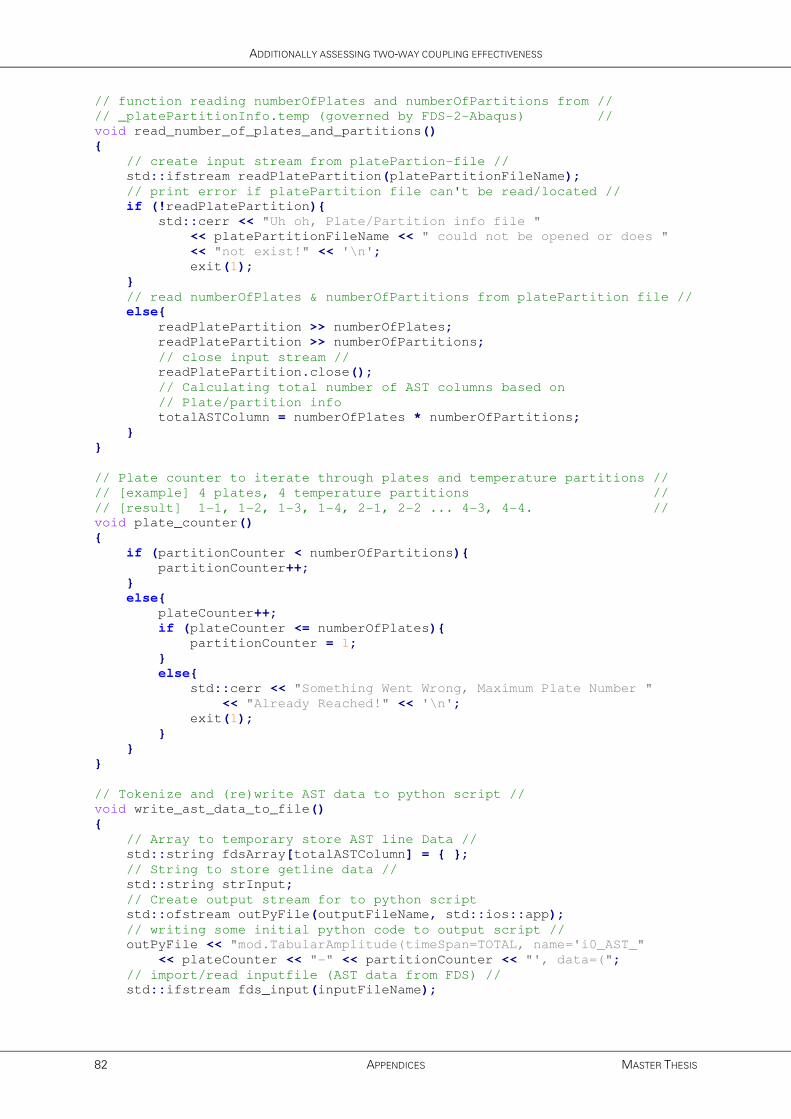
ADDITIONALLY ASSESSING TWO-WAY COUPLING EFFECTIVENESS
82 APPENDICES MASTER THESIS
// function reading numberOfPlates and numberOfPartitions from //
// _platePartitionInfo.temp (governed by FDS-2-Abaqus) //
void read_number_of_plates_and_partitions()
{
// create input stream from platePartion-file //
std::ifstream readPlatePartition(platePartitionFileName);
// print error if platePartition file can't be read/located //
if (!readPlatePartition){
std::cerr << "Uh oh, Plate/Partition info file "
<< platePartitionFileName << " could not be opened or does "
<< "not exist!" << '\n';
exit(1);
}
// read numberOfPlates & numberOfPartitions from platePartition file //
else{
readPlatePartition >> numberOfPlates;
readPlatePartition >> numberOfPartitions;
// close input stream //
readPlatePartition.close();
// Calculating total number of AST columns based on
// Plate/partition info
totalASTColumn = numberOfPlates * numberOfPartitions;
}
}
// Plate counter to iterate through plates and temperature partitions //
// [example] 4 plates, 4 temperature partitions //
// [result] 1-1, 1-2, 1-3, 1-4, 2-1, 2-2 ... 4-3, 4-4. //
void plate_counter()
{
if (partitionCounter < numberOfPartitions){
partitionCounter++;
}
else{
plateCounter++;
if (plateCounter <= numberOfPlates){
partitionCounter = 1;
}
else{
std::cerr << "Something Went Wrong, Maximum Plate Number "
<< "Already Reached!" << '\n';
exit(1);
}
}
}
// Tokenize and (re)write AST data to python script //
void write_ast_data_to_file()
{
// Array to temporary store AST line Data //
std::string fdsArray[totalASTColumn] = { };
// String to store getline data //
std::string strInput;
// Create output stream for to python script
std::ofstream outPyFile(outputFileName, std::ios::app);
// writing some initial python code to output script //
outPyFile << "mod.TabularAmplitude(timeSpan=TOTAL, name='i0_AST_"
<< plateCounter << "-" << partitionCounter << "', data=(";
// import/read inputfile (AST data from FDS) //
std::ifstream fds_input(inputFileName);

FDS-2-ABAQUS: C++ MANAGED AUTOMATED PYTHON SCRIPTED CFD-FEM COUPLING
J.A. FEENSTRA APPENDICES 83
// print error if input file cant be read/located //
if (!fds_input){
std::cerr << "Uh oh, input file " << inputFileName << " could not "
<< "be opened or does not exist!" << '\n';
exit(1);
}
else{
// define seperator for tokenizer //
boost::char_separator<char> sep(",");
// define tokenizer_T1 with separator listed above //
typedef boost::tokenizer\
< boost::char_separator<char> > tokenizer_T1;
// initiate while loop
// this loop continues till end of input file is reached //
while(!fds_input.eof()){
// counter for placing tokens in fdsArray //
int arrayCount=0;
// getline from input file and put in string strInput //
getline(fds_input, strInput);
// statement to check for and skip empty lines //
if (strInput == ""){
continue;
}
// tokenize the 'getline in strInput' //
tokenizer_T1 tok(strInput, sep);
// for loop placing tokens in fdsArray //
for(
tokenizer_T1::iterator token=tok.begin();
token!=tok.end();
++token
){
fdsArray[arrayCount++] = *token;
}
// statement to skip line if first banner line (units) //
if (fdsArray[0] == "s"){
continue;
}
// statement to skip line if second banner line (parameters) //
if (fdsArray[0] == "Time"){
continue;
}
// output time/AST-temperature data to output script //
outPyFile << "(" << fdsArray[0] << ","
<< fdsArray[ioColumnCounter] << ")"<< ",";
}
// finalizing python command with closing brackets //
outPyFile << "))" << '\n';
outPyFile.close();
// output append-info to console //
std::cout << "Successfully appended AST data for Plate "
<< plateCounter << "-" << partitionCounter << " to "
<< outputFileName << '\n';
}
}
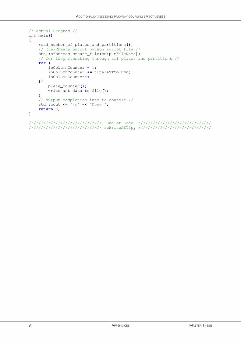
ADDITIONALLY ASSESSING TWO-WAY COUPLING EFFECTIVENESS
84 APPENDICES MASTER THESIS
// Actual Program //
int main()
{
read_number_of_plates_and_partitions();
// (re)Create output python script file //
std::ofstream create_file(outputFileName);
// for loop iterating through all plates and partitions //
for (
ioColumnCounter = 1;
ioColumnCounter <= totalASTColumn;
ioColumnCounter++
){
plate_counter();
write_ast_data_to_file();
}
// output completion info to console //
std::cout << '\n' << "Done!";
return 0;
}
////////////////////////////// End of Code //////////////////////////////
////////////////////////////// reWriteAST2py //////////////////////////////

FDS-2-ABAQUS: C++ MANAGED AUTOMATED PYTHON SCRIPTED CFD-FEM COUPLING
J.A. FEENSTRA APPENDICES 85
APPENDIX D3 – UPGEOMFDS: C++ SOURCE CODE
///////////////////////////////////////////////////////////////////////////
// Name: upGeomFDS //
// //
// Description: This program creates a FDS input file for the current //
// iteration. Basically it copies the basicSetupFile, //
// FDS_BasicSetup.fds, to a new input file, FDS_script.fds, //
// and appends input lines defining the next iteration and //
// plate failure devices. The iteration parameters are read //
// from temporary file _iterationCounter.temp and the plate //
// failure parameters from _plateFailure.log. Both of which //
// are managed by 'Master Program' FDS-2-Abaqus. //
// //
// Input: FDS_BasicSetup.fds //
// _iterationCounter.temp //
// _plateFailure.log //
// //
// Output: FDS_Script.fds //
// //
// Required iterationCounter //
// Parameters: iterationSize //
// totalSimulationDuration //
// failedPlateNumber //
// failureTimePoint //
// plateFailureBool //
// //
///////////////////////////////////////////////////////////////////////////
// Version 1.0 by J.A.Feenstra //
// August 2016 [email protected] //
///////////////////////////////////////////////////////////////////////////
/////////////////////////////// Begin Code ////////////////////////////////
// Import Libraries //
#include <iostream>
#include <string>
#include <fstream>
#include <cstdlib>
// Define String Parameters //
// input filename for *.fds file containing basic FDS model setup //
std::string basicSetupFileName = "FDS_BasicSetup.fds";
// output filename for updated FDS script //
std::string scriptFileName = "FDS_Script.fds";
// input filename for iterationCounter containing iteration data //
std::string counterFileName = "_iterationCounter.temp";
// input filename for temporary file containing plate/partition info //
std::string platePartitionFileName = "_platePartitionInfo.temp";
// input filename for logfile containing failure-info //
std::string plateFailureFileName = "_plateFailure.log";
// Define Integer Parameters //
// read from counterFileName (_iterationCounter.temp) //
// managed by FDS-2-Abaqus //
int iterationCounter(0);
int iterationSize(50);
int totalSimulationDuration(100);

ADDITIONALLY ASSESSING TWO-WAY COUPLING EFFECTIVENESS
86 APPENDICES MASTER THESIS
// read from platePartitionFileName (_platePartitionInfo.temp) //
// managed by FDS-2-Abaqus //
int numberOfPlates(1); // is read from platePartitionFileName
int numberOfPartitions(1);
// read from plateFailureFileName (_plateFailure.log) //
// managed by FDS-2-Abaqus //
int failedPlateNumber(0);
int failureTimePoint(0);
// calculated based on iterationInfo //
int currentIterationSetPoint(0);
int nextIterationSetPoint(50);
// Define Boolean Parameters //
// read from plateFailureFileName (_plateFailure.log) //
// managed by FDS-2-Abaqus //
bool plateFailureBool;
// function importing iteration-info from //
// _platePartitionInfo.temp (managed by FDS-2-Abaqus) //
void read_current_iteration()
{
// create input stream from iteration counter file //
std::ifstream readCounter(counterFileName);
// print error if iterationCounter file can't be read/located //
if (!readCounter){
std::cerr << "Uh oh, iteration counter file " << counterFileName
<< " could not be opened or does not exist!" << '\n';
exit(1);
}
// read/write integers from counterFile to parameters //
else{
readCounter >> iterationCounter;
readCounter >> iterationSize;
readCounter >> totalSimulationDuration;
// close input stream //
readCounter.close();
}
}
// function importing plate/partition info from //
// _platePartitionInfo.temp (managed by FDS-2-Abaqus) //
void read_number_of_plates_and_partitions()
{
// create input stream from plate/partition file //
std::ifstream readPlatePartition(platePartitionFileName);
// print error if iterationCounter file can't be read/located //
if (!readPlatePartition){
std::cerr << "Uh oh, Plate/Partition info file "
<< platePartitionFileName
<< " could not be opened or does not exist!" << '\n';
exit(1);
}
// read/write integers from plate/partition file to parameters //
else{
readPlatePartition >> numberOfPlates;
readPlatePartition >> numberOfPartitions;
readPlatePartition.close();
}
}
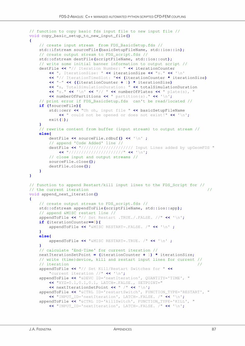
FDS-2-ABAQUS: C++ MANAGED AUTOMATED PYTHON SCRIPTED CFD-FEM COUPLING
J.A. FEENSTRA APPENDICES 87
// function to copy basic fds input file to new input file //
void copy_basic_setup_to_new_input_file()
{
// create input stream from FDS_BasicSetup.fds //
std::ifstream sourceFile(basicSetupFileName, std::ios::in);
// create output stream to FDS_script.fds //
std::ofstream destFile(scriptFileName, std::ios::out);
// write some initial banner information to output script //
destFile << "// Iteration Number: " << iterationCounter
<< ", IterationSize: " << iterationSize << "s." << '\n'
<< "// IterationTimeSlot: "<< (iterationCounter * iterationSize)
<< "-" << ((iterationCounter + 1) * iterationSize)
<< "s, TotalSimulationDuration: " << totalSimulationDuration
<< "s." << '\n' << "// " << numberOfPlates << " plate(s), "
<< numberOfPartitions << " partition(s)." << '\n';
// print error if FDS_BasicSetup.fds can't be read/located //
if (!sourceFile){
std::cerr << "Uh oh, input file " << basicSetupFileName
<< " could not be opened or does not exist!" << '\n';
exit(1);
}
// rewrite content from buffer (input stream) to output stream //
else{
destFile << sourceFile.rdbuf() << '\n' ;
// append 'Code Added' line //
destFile << "///////////////////// Input Lines added by upGeomFDS "
<< "//////////////////////" << '\n';
// close input and output streams //
sourceFile.close();
destFile.close();
}
}
// function to append Restart/kill input lines to the FDS_Script for //
// the current iteration //
void append_next_iteration()
{
// create output stream to FDS_script.fds //
std::ofstream appendToFile(scriptFileName, std::ios::app);
// append &MISC restart line //
appendToFile << "// Set Restart .TRUE./.FALSE. //" << '\n';
if (iterationCounter==0){
appendToFile << "&MISC RESTART=.FALSE. /" << '\n' ;
}
else{
appendToFile << "&MISC RESTART=.TRUE. /" << '\n' ;
}
// calculate 'End-Time' for current iteration //
nextIterationSetPoint = (iterationCounter + 1) * iterationSize;
// write (time)device, kill and restart input lines for current //
// iteration //
appendToFile << "// Set Kill/Restart Switches for " <<
"current iteration //" << '\n';
appendToFile << "&DEVC ID='nextIteration', QUANTITY='TIME', "
<< "XYZ=0.1,0.1,0.1, LATCH=.FALSE., SETPOINT="
<< nextIterationSetPoint << " /" << '\n';
appendToFile << "&CTRL ID='restartSwitch', FUNCTION_TYPE='RESTART', "
<< "INPUT_ID='nextIteration', LATCH=.FALSE. /" << '\n';
appendToFile << "&CTRL ID='killSwitch', FUNCTION_TYPE='KILL', "
<< "INPUT_ID='nextIteration', LATCH=.FALSE. /" << '\n';
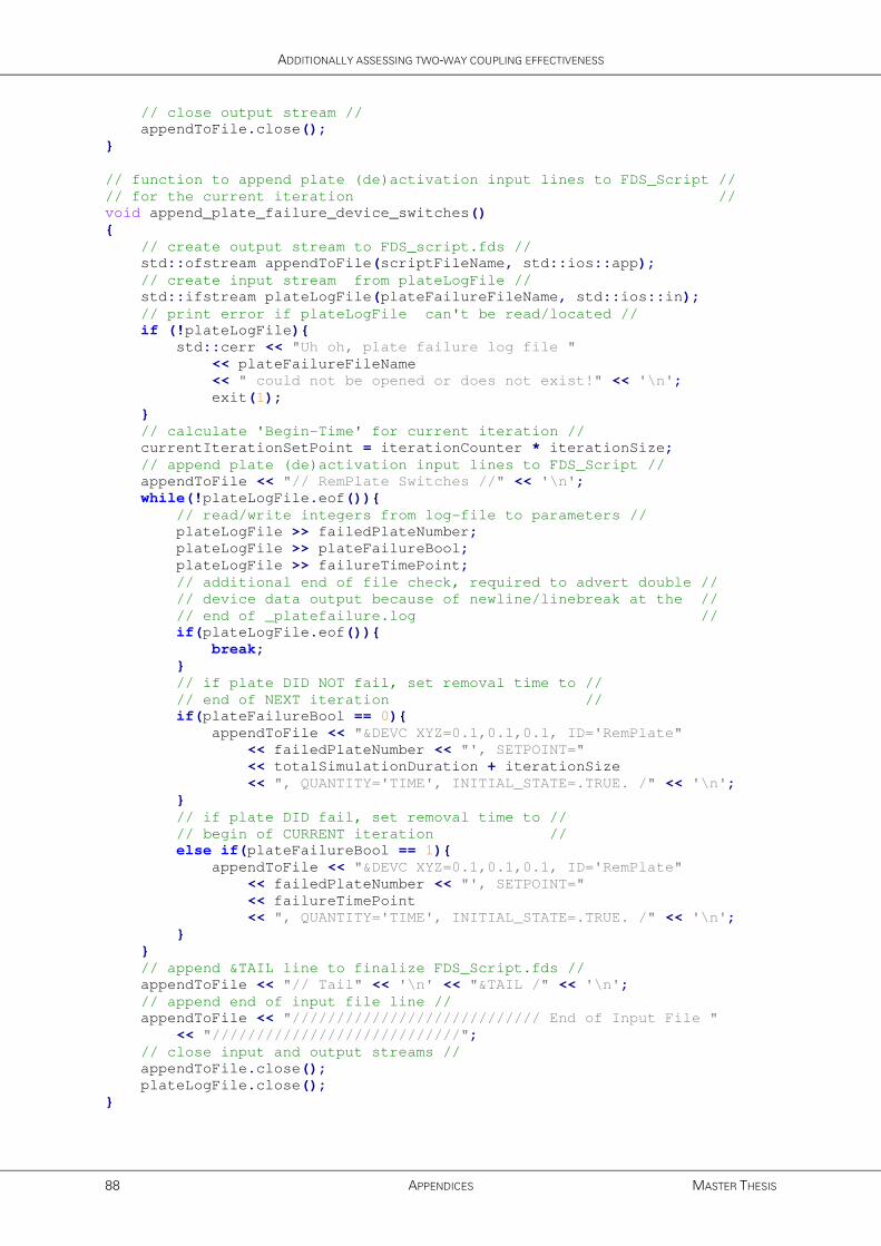
ADDITIONALLY ASSESSING TWO-WAY COUPLING EFFECTIVENESS
88 APPENDICES MASTER THESIS
// close output stream //
appendToFile.close();
}
// function to append plate (de)activation input lines to FDS_Script //
// for the current iteration //
void append_plate_failure_device_switches()
{
// create output stream to FDS_script.fds //
std::ofstream appendToFile(scriptFileName, std::ios::app);
// create input stream from plateLogFile //
std::ifstream plateLogFile(plateFailureFileName, std::ios::in);
// print error if plateLogFile can't be read/located //
if (!plateLogFile){
std::cerr << "Uh oh, plate failure log file "
<< plateFailureFileName
<< " could not be opened or does not exist!" << '\n';
exit(1);
}
// calculate 'Begin-Time' for current iteration //
currentIterationSetPoint = iterationCounter * iterationSize;
// append plate (de)activation input lines to FDS_Script //
appendToFile << "// RemPlate Switches //" << '\n';
while(!plateLogFile.eof()){
// read/write integers from log-file to parameters //
plateLogFile >> failedPlateNumber;
plateLogFile >> plateFailureBool;
plateLogFile >> failureTimePoint;
// additional end of file check, required to advert double //
// device data output because of newline/linebreak at the //
// end of _platefailure.log //
if(plateLogFile.eof()){
break;
}
// if plate DID NOT fail, set removal time to //
// end of NEXT iteration //
if(plateFailureBool == 0){
appendToFile << "&DEVC XYZ=0.1,0.1,0.1, ID='RemPlate"
<< failedPlateNumber << "', SETPOINT="
<< totalSimulationDuration + iterationSize
<< ", QUANTITY='TIME', INITIAL_STATE=.TRUE. /" << '\n';
}
// if plate DID fail, set removal time to //
// begin of CURRENT iteration //
else if(plateFailureBool == 1){
appendToFile << "&DEVC XYZ=0.1,0.1,0.1, ID='RemPlate"
<< failedPlateNumber << "', SETPOINT="
<< failureTimePoint
<< ", QUANTITY='TIME', INITIAL_STATE=.TRUE. /" << '\n';
}
}
// append &TAIL line to finalize FDS_Script.fds //
appendToFile << "// Tail" << '\n' << "&TAIL /" << '\n';
// append end of input file line //
appendToFile << "//////////////////////////// End of Input File "
<< "////////////////////////////";
// close input and output streams //
appendToFile.close();
plateLogFile.close();
}

FDS-2-ABAQUS: C++ MANAGED AUTOMATED PYTHON SCRIPTED CFD-FEM COUPLING
J.A. FEENSTRA APPENDICES 89
// function outputting (simple) completion message to console //
void process_completed()
{
std::cout << "[ [ [upGeomFDS] ] ]" << '\n'
<< "Successfully updated FDS input file for iteration: "
<< iterationCounter << '\n' << '\n';
}
// Actual Program //
int main()
{
read_current_iteration();
read_number_of_plates_and_partitions();
copy_basic_setup_to_new_input_file();
append_next_iteration();
append_plate_failure_device_switches();
process_completed();
return 0;
}
/////////////////////////////// End of Code ///////////////////////////////
/////////////////////////////// upGeomFDS ///////////////////////////////

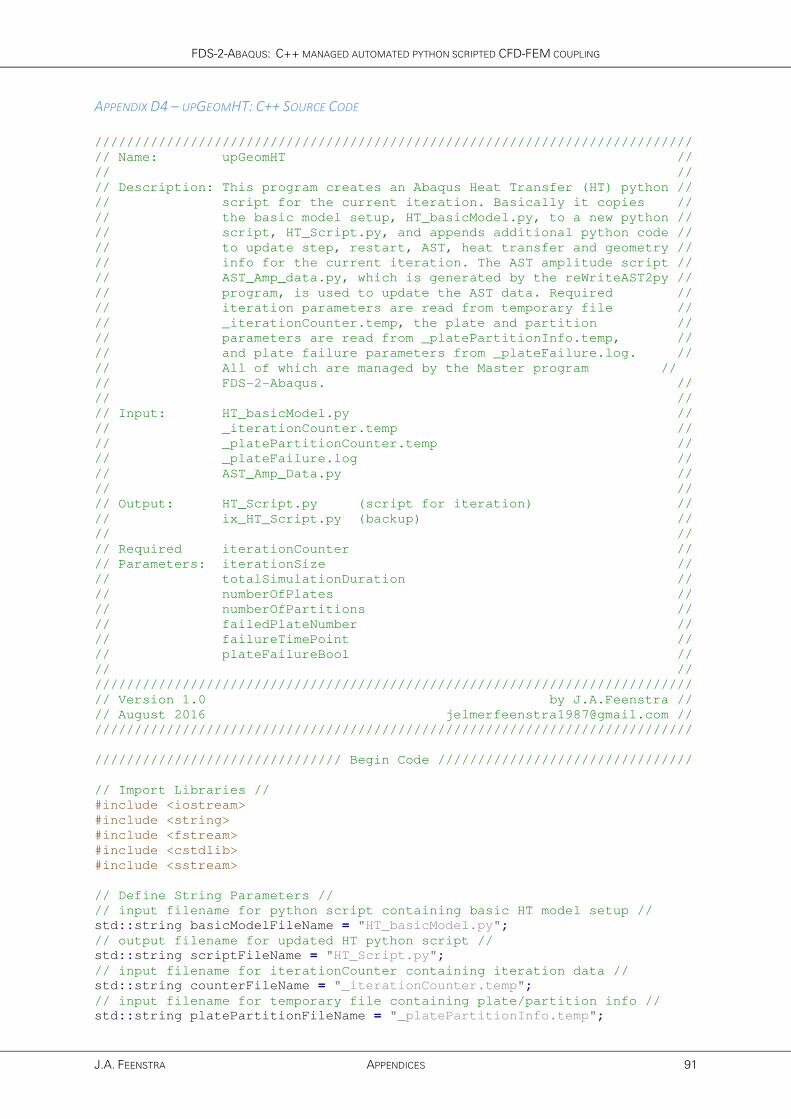
FDS-2-ABAQUS: C++ MANAGED AUTOMATED PYTHON SCRIPTED CFD-FEM COUPLING
J.A. FEENSTRA APPENDICES 91
APPENDIX D4 – UPGEOMHT: C++ SOURCE CODE
///////////////////////////////////////////////////////////////////////////
// Name: upGeomHT //
// //
// Description: This program creates an Abaqus Heat Transfer (HT) python //
// script for the current iteration. Basically it copies //
// the basic model setup, HT_basicModel.py, to a new python //
// script, HT_Script.py, and appends additional python code //
// to update step, restart, AST, heat transfer and geometry //
// info for the current iteration. The AST amplitude script //
// AST_Amp_data.py, which is generated by the reWriteAST2py //
// program, is used to update the AST data. Required //
// iteration parameters are read from temporary file //
// _iterationCounter.temp, the plate and partition //
// parameters are read from _platePartitionInfo.temp, //
// and plate failure parameters from _plateFailure.log. //
// All of which are managed by the Master program //
// FDS-2-Abaqus. //
// //
// Input: HT_basicModel.py //
// _iterationCounter.temp //
// _platePartitionCounter.temp //
// _plateFailure.log //
// AST_Amp_Data.py //
// //
// Output: HT_Script.py (script for iteration) //
// ix_HT_Script.py (backup) //
// //
// Required iterationCounter //
// Parameters: iterationSize //
// totalSimulationDuration //
// numberOfPlates //
// numberOfPartitions //
// failedPlateNumber //
// failureTimePoint //
// plateFailureBool //
// //
///////////////////////////////////////////////////////////////////////////
// Version 1.0 by J.A.Feenstra //
// August 2016 [email protected] //
///////////////////////////////////////////////////////////////////////////
/////////////////////////////// Begin Code ////////////////////////////////
// Import Libraries //
#include <iostream>
#include <string>
#include <fstream>
#include <cstdlib>
#include <sstream>
// Define String Parameters //
// input filename for python script containing basic HT model setup //
std::string basicModelFileName = "HT_basicModel.py";
// output filename for updated HT python script //
std::string scriptFileName = "HT_Script.py";
// input filename for iterationCounter containing iteration data //
std::string counterFileName = "_iterationCounter.temp";
// input filename for temporary file containing plate/partition info //
std::string platePartitionFileName = "_platePartitionInfo.temp";
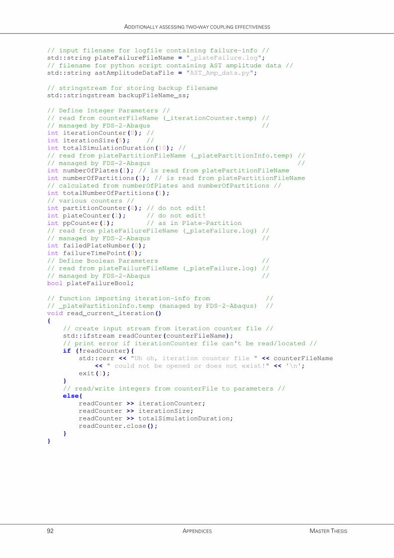
ADDITIONALLY ASSESSING TWO-WAY COUPLING EFFECTIVENESS
92 APPENDICES MASTER THESIS
// input filename for logfile containing failure-info //
std::string plateFailureFileName = "_plateFailure.log";
// filename for python script containing AST amplitude data //
std::string astAmplitudeDataFile = "AST_Amp_data.py";
// stringstream for storing backup filename
std::stringstream backupFileName_ss;
// Define Integer Parameters //
// read from counterFileName (_iterationCounter.temp) //
// managed by FDS-2-Abaqus //
int iterationCounter(0); //
int iterationSize(5); //
int totalSimulationDuration(10); //
// read from platePartitionFileName (_platePartitionInfo.temp) //
// managed by FDS-2-Abaqus //
int numberOfPlates(1); // is read from platePartitionFileName
int numberOfPartitions(1); // is read from platePartitionFileName
// calculated from numberOfPlates and numberOfPartitions //
int totalNumberOfPartitions(1);
// various counters //
int partitionCounter(0); // do not edit!
int plateCounter(1); // do not edit!
int ppCounter(1); // as in Plate-Partition
// read from plateFailureFileName (_plateFailure.log) //
// managed by FDS-2-Abaqus //
int failedPlateNumber(0);
int failureTimePoint(0);
// Define Boolean Parameters //
// read from plateFailureFileName (_plateFailure.log) //
// managed by FDS-2-Abaqus //
bool plateFailureBool;
// function importing iteration-info from //
// _platePartitionInfo.temp (managed by FDS-2-Abaqus) //
void read_current_iteration()
{
// create input stream from iteration counter file //
std::ifstream readCounter(counterFileName);
// print error if iterationCounter file can't be read/located //
if (!readCounter){
std::cerr << "Uh oh, iteration counter file " << counterFileName
<< " could not be opened or does not exist!" << '\n';
exit(1);
}
// read/write integers from counterFile to parameters //
else{
readCounter >> iterationCounter;
readCounter >> iterationSize;
readCounter >> totalSimulationDuration;
readCounter.close();
}
}

FDS-2-ABAQUS: C++ MANAGED AUTOMATED PYTHON SCRIPTED CFD-FEM COUPLING
J.A. FEENSTRA APPENDICES 93
// function importing plate/partition info from //
// _platePartitionInfo.temp (managed by FDS-2-Abaqus) //
void read_number_of_plates_and_partitions()
{
// create input stream from plate/partition file //
std::ifstream readPlatePartition(platePartitionFileName);
// print error if iterationCounter file can't be read/located //
if (!readPlatePartition){
std::cerr << "Uh oh, Plate/Partition info file "
<< platePartitionFileName
<< " could not be opened or does not exist!" << '\n';
exit(1);
}
// read/write integers from plate/partition file to parameters //
else{
readPlatePartition >> numberOfPlates;
readPlatePartition >> numberOfPartitions;
readPlatePartition.close();
}
}
// Plate counter to iterate through plates and temperature partitions //
// [example] 4 plates, 4 temperature partitions //
// [result] 1-1, 1-2, 1-3, 1-4, 2-1, 2-2 ... 4-3, 4-4. //
void plate_counter()
{
if (partitionCounter < numberOfPartitions){
partitionCounter++;
}
else{
plateCounter++;
if (plateCounter <= numberOfPlates){
partitionCounter = 1;
}
}
}
// function to copy basic HT model python script to a new script //
// for the current iteration //
void copy_basic_model_to_new_py()
{
// create input stream from HT_basicModel.py //
std::ifstream sourceFile(basicModelFileName, std::ios::in);
// create output stream to HT_script.py //
std::ofstream destFile(scriptFileName, std::ios::out);
// write some initial banner information to output script //
destFile << "# Iteration Number: " << iterationCounter
<< ", IterationSize: " << iterationSize << "s." << '\n'
<< "# IterationTimeSlot: "<< (iterationCounter * iterationSize)
<< "-" << ((iterationCounter + 1) * iterationSize)
<< "s, TotalSimulationDuration: " << totalSimulationDuration
<< "s." << '\n' << "# " << numberOfPlates<< " plate(s), "
<< numberOfPartitions << " partition(s)."<< '\n';
// print error if HT_basicModel.py can't be read/located //
if (!sourceFile){
std::cerr << "Uh oh, input file " << basicModelFileName
<< " could not be opened or does not exist!" << '\n';
exit(1);
}
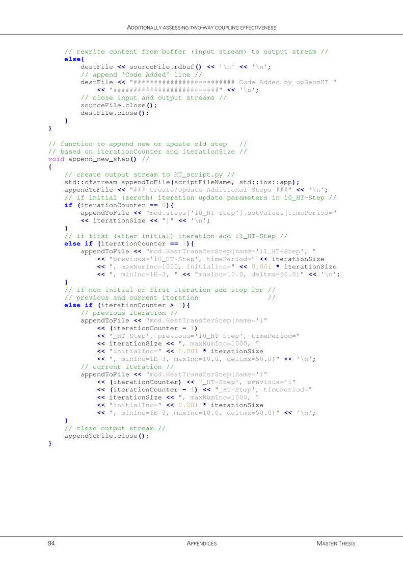
ADDITIONALLY ASSESSING TWO-WAY COUPLING EFFECTIVENESS
94 APPENDICES MASTER THESIS
// rewrite content from buffer (input stream) to output stream //
else{
destFile << sourceFile.rdbuf() << '\n' << '\n';
// append 'Code Added' line //
destFile << "######################### Code Added by upGeomHT "
<< "##########################" << '\n';
// close input and output streams //
sourceFile.close();
destFile.close();
}
}
// function to append new or update old step //
// based on iterationCounter and iterationSize //
void append_new_step() //
{
// create output stream to HT_script.py //
std::ofstream appendToFile(scriptFileName, std::ios::app);
appendToFile << "### Create/Update Additional Steps ###" << '\n';
// if initial (zeroth) iteration update parameters in i0_HT-Step //
if (iterationCounter == 0){
appendToFile << "mod.steps['i0_HT-Step'].setValues(timePeriod="
<< iterationSize << ")" << '\n';
}
// if first (after initial) iteration add i1_HT-Step //
else if (iterationCounter == 1){
appendToFile << "mod.HeatTransferStep(name='i1_HT-Step', "
<< "previous='i0_HT-Step', timePeriod=" << iterationSize
<< ", maxNumInc=1000, initialInc=" << 0.001 * iterationSize
<< ", minInc=1E-3, " << "maxInc=10.0, deltmx=50.0)" << '\n';
}
// if non initial or first iteration add step for //
// previous and current iteration //
else if (iterationCounter > 1){
// previous iteration //
appendToFile << "mod.HeatTransferStep(name='i"
<< (iterationCounter - 1)
<< "_HT-Step', previous='i0_HT-Step', timePeriod="
<< iterationSize << ", maxNumInc=1000, "
<< "initialInc=" << 0.001 * iterationSize
<< ", minInc=1E-3, maxInc=10.0, deltmx=50.0)" << '\n';
// current iteration //
appendToFile << "mod.HeatTransferStep(name='i"
<< (iterationCounter) << "_HT-Step', previous='i"
<< (iterationCounter - 1) << "_HT-Step', timePeriod="
<< iterationSize << ", maxNumInc=1000, "
<< "initialInc=" << 0.001 * iterationSize
<< ", minInc=1E-3, maxInc=10.0, deltmx=50.0)" << '\n';
}
// close output stream //
appendToFile.close();
}

FDS-2-ABAQUS: C++ MANAGED AUTOMATED PYTHON SCRIPTED CFD-FEM COUPLING
J.A. FEENSTRA APPENDICES 95
// function to append code to read the restart file from previous //
// iteration and request a new restart file for this iteration //
void append_restart_job_step()
{
// create output stream to HT_script.py //
std::ofstream appendToFile(scriptFileName, std::ios::app);
appendToFile << "### Define Restart Job/Step ###" << '\n';
// if non-zeroth iteration then append python code to read restart //
// file from previous iteration and request a new restart file //
// for this iteration //
if (iterationCounter > 0){
appendToFile << "mod.setValues(restartJob='i"
<< (iterationCounter - 1) << "_HT-Job', restartStep='i"
<< (iterationCounter - 1) << "_HT-Step')" << '\n';
appendToFile << "### Request Restart File for New Step ###"<< '\n';
appendToFile << "mod.steps['i" << iterationCounter
<< "_HT-Step'].Restart(frequency=0, numberIntervals=1, "
<< "overlay=ON, timeMarks=OFF)" << '\n';
}
// if zeroth iteration then no additional code is written //
// (only a comment) //
else if (iterationCounter == 0){
appendToFile << "#no additional restart information is written "
<< "since it is the initial (zero'th) iteration" << '\n';
}
// print error if iteration counter is negative //
// (should never occur) //
else if (iterationCounter < 0){
std::cerr << "Uh oh, iteration counter is negative check "
<< counterFileName << '\n';
exit(1);
}
// close output stream //
appendToFile.close();
}
// function to append python code to update AST tabular amplitude data //
// and defining convective and radiative heat transfer //
void append_update_ConRad_AST_Data()
{
// create output stream to HT_script.py //
std::ofstream appendToFile(scriptFileName, std::ios::app);
appendToFile << "### Update ConRad and AST Data ###" << '\n';
appendToFile << "imp = mod.TabularAmplitude" << '\n';
// code to update AST data (AST_Amp_Data.py) //
// NOTE: this python-command refers to a relative path //
appendToFile << "execfile(r'../" << astAmplitudeDataFile
<< "', __main__.__dict__)" << '\n';
// calculate total number of partitions to use in for loop //
totalNumberOfPartitions = numberOfPlates * numberOfPartitions;
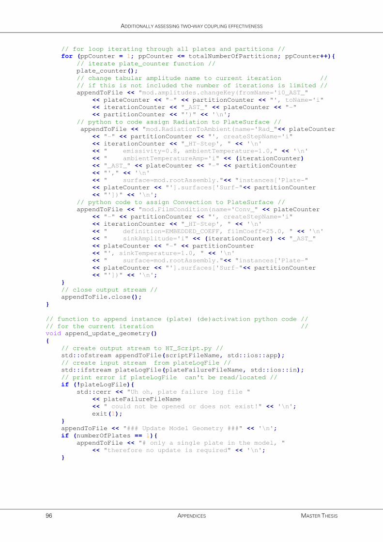
ADDITIONALLY ASSESSING TWO-WAY COUPLING EFFECTIVENESS
96 APPENDICES MASTER THESIS
// for loop iterating through all plates and partitions //
for (ppCounter = 1; ppCounter <= totalNumberOfPartitions; ppCounter++){
// iterate plate_counter function //
plate_counter();
// change tabular amplitude name to current iteration //
// if this is not included the number of iterations is limited //
appendToFile << "mod.amplitudes.changeKey(fromName='i0_AST_"
<< plateCounter << "-" << partitionCounter << "', toName='i"
<< iterationCounter << "_AST_" << plateCounter << "-"
<< partitionCounter << "')" << '\n';
// python to code assign Radiation to PlateSurface //
appendToFile << "mod.RadiationToAmbient(name='Rad_"<< plateCounter
<< "-" << partitionCounter << "', createStepName='i"
<< iterationCounter << "_HT-Step', " << '\n'
<< " emissivity=0.8, ambientTemperature=1.0," << '\n'
<< " ambientTemperatureAmp='i" << (iterationCounter)
<< "_AST_" << plateCounter << "-" << partitionCounter
<< "'," << '\n'
<< " surface=mod.rootAssembly."<< "instances['Plate-"
<< plateCounter << "'].surfaces['Surf-"<< partitionCounter
<< "'])" << '\n';
// python code to assign Convection to PlateSurface //
appendToFile << "mod.FilmCondition(name='Conv_" << plateCounter
<< "-" << partitionCounter << "', createStepName='i"
<< iterationCounter << "_HT-Step', " << '\n'
<< " definition=EMBEDDED_COEFF, filmCoeff=25.0, " << '\n'
<< " sinkAmplitude='i" << (iterationCounter) << "_AST_"
<< plateCounter << "-" << partitionCounter
<< "', sinkTemperature=1.0, " << '\n'
<< " surface=mod.rootAssembly."<< "instances['Plate-"
<< plateCounter << "'].surfaces['Surf-"<< partitionCounter
<< "'])" << '\n';
}
// close output stream //
appendToFile.close();
}
// function to append instance (plate) (de)activation python code //
// for the current iteration //
void append_update_geometry()
{
// create output stream to HT_Script.py //
std::ofstream appendToFile(scriptFileName, std::ios::app);
// create input stream from plateLogFile //
std::ifstream plateLogFile(plateFailureFileName, std::ios::in);
// print error if plateLogFile can't be read/located //
if (!plateLogFile){
std::cerr << "Uh oh, plate failure log file "
<< plateFailureFileName
<< " could not be opened or does not exist!" << '\n';
exit(1);
}
appendToFile << "### Update Model Geometry ###" << '\n';
if (numberOfPlates == 1){
appendToFile << "# only a single plate in the model, "
<< "therefore no update is required" << '\n';
}

FDS-2-ABAQUS: C++ MANAGED AUTOMATED PYTHON SCRIPTED CFD-FEM COUPLING
J.A. FEENSTRA APPENDICES 97
else if (numberOfPlates > 1){
// while loop updating through input file //
while(!plateLogFile.eof()){
plateLogFile >> failedPlateNumber;
plateLogFile >> plateFailureBool;
plateLogFile >> failureTimePoint;
// additional end of file check, required to advert //
// duplicate plate deactivation code because of //
// newline/linebreak at the end of _platefailure.log //
if(plateLogFile.eof()){
break;
}
// if plate DID NOT fail, continue //
if(plateFailureBool==0){
// nothing really happens here xD //
continue;
}
// if plate DID fail, append python code to //
// deactivate instance (= remove plate) //
else{
appendToFile << "thisPlate = mod.rootAssembly.instances"
<< "['Plate-" << failedPlateNumber
<< "'].sets['Plate-Area']" << '\n';
appendToFile << "mod.ModelChange(activeInStep=False, "
<< "createStepName='i" << iterationCounter
<< "_HT-Step', includeStrain=False, name='deActPlate-"
<< failedPlateNumber << "', region=thisPlate)" << '\n';
}
}
// just some info //
appendToFile << "# If empty: No plates failed this iteration "
<< "- Still Going Strong!" << '\n';
}
// close input and output streams //
appendToFile.close();
plateLogFile.close();
}
// function appending python code to create and run (restart) job //
// 'normal' job for initial (zeroth) iteration, restart for other //
void append_create_and_run_job()
{
// create output stream to HT_Script.py //
std::ofstream appendToFile(scriptFileName, std::ios::app);
appendToFile << "### Create and Run Job ###" << '\n';
// if initial (zeroth) iteration append standard Job python code //
if (iterationCounter == 0){
appendToFile << "mdb.Job(name='i0_HT-Job', model='Model-1')"
<< '\n';
}
// if NON-initial iteration append restart Job python code //
else if (iterationCounter > 0){
appendToFile << "mdb.Job(name='i" << iterationCounter
<< "_HT-Job', model='Model-1', type=RESTART)" << '\n';
}
// append submit and run job python code to script //
appendToFile << "mdb.jobs['i" << iterationCounter
<< "_HT-Job'].submit(consistencyChecking=OFF)" << '\n';
appendToFile << "mdb.jobs['i" << iterationCounter
<< "_HT-Job'].waitForCompletion()" << '\n';

ADDITIONALLY ASSESSING TWO-WAY COUPLING EFFECTIVENESS
98 APPENDICES MASTER THESIS
// append end of script line //
appendToFile << "############################## "
<< "End-Of-Script ##############################";
// close output stream //
appendToFile.close();
}
// function to backup HT_Script for current iteration //
// rewriting script into file named ix_HT_Script.py //
void create_backup_for_current_iteration()
{
// create input stream from HT_Script.py //
std::ifstream sourceFile(scriptFileName, std::ios::in);
// write backup filename to stringstream
backupFileName_ss.clear();
backupFileName_ss << "i" << iterationCounter << "_HT_Script.py";
// create output stream to HT_Script.py //
std::ofstream destFile(backupFileName_ss.str(), std::ios::out);
// print error if HT_Script.py can't be read/located //
if (!sourceFile){
std::cerr << "Uh oh, input file " << scriptFileName
<< " could not be opened or does not exist!" << '\n';
exit(1);
}
// rewrite content from buffer (input stream) to output stream //
else{
destFile << sourceFile.rdbuf() << '\n';
// close input and output streams //
sourceFile.close();
destFile.close();
}
}
// function outputting (simple) completion message to console //
void process_completed()
{
std::cout << "[ [ [upGeomHT] ] ]" << '\n'
<< "Successfully updated HT python script for iteration: "
<< iterationCounter << '\n' << '\n';
}
int main()
{
read_current_iteration();
read_number_of_plates_and_partitions();
copy_basic_model_to_new_py();
append_new_step();
append_restart_job_step();
append_update_ConRad_AST_Data();
append_update_geometry();
append_create_and_run_job();
create_backup_for_current_iteration();
process_completed();
return 0;
}
/////////////////////////////// End of Code ///////////////////////////////
/////////////////////////////// upGeomHT ///////////////////////////////
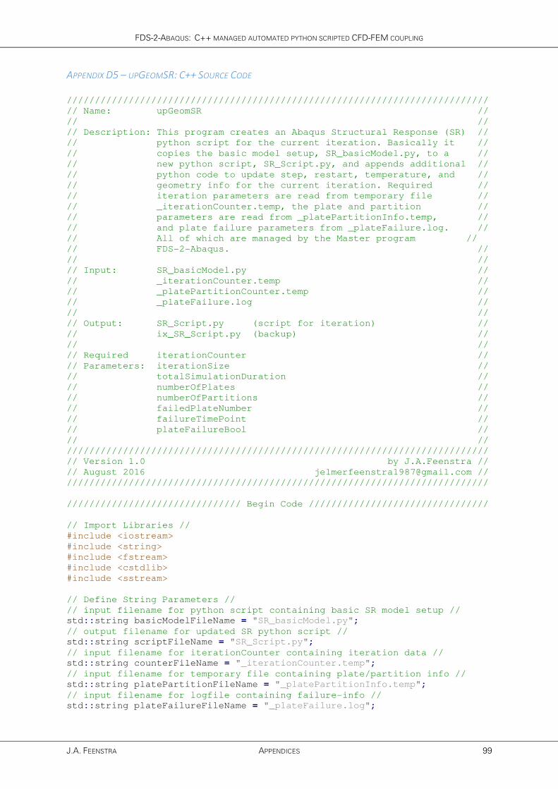
FDS-2-ABAQUS: C++ MANAGED AUTOMATED PYTHON SCRIPTED CFD-FEM COUPLING
J.A. FEENSTRA APPENDICES 99
APPENDIX D5 – UPGEOMSR: C++ SOURCE CODE
///////////////////////////////////////////////////////////////////////////
// Name: upGeomSR //
// //
// Description: This program creates an Abaqus Structural Response (SR) //
// python script for the current iteration. Basically it //
// copies the basic model setup, SR_basicModel.py, to a //
// new python script, SR_Script.py, and appends additional //
// python code to update step, restart, temperature, and //
// geometry info for the current iteration. Required //
// iteration parameters are read from temporary file //
// _iterationCounter.temp, the plate and partition //
// parameters are read from _platePartitionInfo.temp, //
// and plate failure parameters from _plateFailure.log. //
// All of which are managed by the Master program //
// FDS-2-Abaqus. //
// //
// Input: SR_basicModel.py //
// _iterationCounter.temp //
// _platePartitionCounter.temp //
// _plateFailure.log //
// //
// Output: SR_Script.py (script for iteration) //
// ix_SR_Script.py (backup) //
// //
// Required iterationCounter //
// Parameters: iterationSize //
// totalSimulationDuration //
// numberOfPlates //
// numberOfPartitions //
// failedPlateNumber //
// failureTimePoint //
// plateFailureBool //
// //
///////////////////////////////////////////////////////////////////////////
// Version 1.0 by J.A.Feenstra //
// August 2016 [email protected] //
///////////////////////////////////////////////////////////////////////////
/////////////////////////////// Begin Code ////////////////////////////////
// Import Libraries //
#include <iostream>
#include <string>
#include <fstream>
#include <cstdlib>
#include <sstream>
// Define String Parameters //
// input filename for python script containing basic SR model setup //
std::string basicModelFileName = "SR_basicModel.py";
// output filename for updated SR python script //
std::string scriptFileName = "SR_Script.py";
// input filename for iterationCounter containing iteration data //
std::string counterFileName = "_iterationCounter.temp";
// input filename for temporary file containing plate/partition info //
std::string platePartitionFileName = "_platePartitionInfo.temp";
// input filename for logfile containing failure-info //
std::string plateFailureFileName = "_plateFailure.log";

ADDITIONALLY ASSESSING TWO-WAY COUPLING EFFECTIVENESS
100 APPENDICES MASTER THESIS
// stringstream for storing backup filename
std::stringstream backupFileName_ss;
// Define Integer Parameters //
// read from counterFileName (_iterationCounter.temp) //
// managed by FDS-2-Abaqus //
int iterationCounter(0);
int iterationSize(5);
int totalSimulationDuration(10);
// read from platePartitionFileName (_platePartitionInfo.temp) //
// managed by FDS-2-Abaqus //
int numberOfPlates(1); // is read from platePartitionFileName
int numberOfPartitions(1);
// read from plateFailureFileName (_plateFailure.log) //
// managed by FDS-2-Abaqus //
int failedPlateNumber(0); //
int failureTimePoint(0);
// Define Boolean Parameters //
// read from plateFailureFileName (_plateFailure.log) //
// managed by FDS-2-Abaqus //
bool plateFailureBool;
// function importing iteration-info from //
// _platePartitionInfo.temp (managed by FDS-2-Abaqus) //
void read_current_iteration()
{
// create input stream from iteration counter file //
std::ifstream readCounter(counterFileName);
// print error if iterationCounter file can't be read/located //
if (!readCounter){
std::cerr << "Uh oh, iteration counter file "
<< counterFileName
<< " could not be opened or does not exist!" << '\n';
exit(1);
}
// read/write integers from counterFile to parameters //
else{
readCounter >> iterationCounter;
readCounter >> iterationSize;
readCounter >> totalSimulationDuration;
readCounter.close();
}
}
// function importing plate/partition info from //
// _platePartitionInfo.temp (managed by FDS-2-Abaqus) //
void read_number_of_plates_and_partitions()
{
// create input stream from plate/partition file //
std::ifstream readPlatePartition(platePartitionFileName);
// print error if iterationCounter file can't be read/located //
if (!readPlatePartition){
std::cerr << "Uh oh, Plate/Partition info file "
<< platePartitionFileName
<< " could not be opened or does not exist!" << '\n';
exit(1);
}

FDS-2-ABAQUS: C++ MANAGED AUTOMATED PYTHON SCRIPTED CFD-FEM COUPLING
J.A. FEENSTRA APPENDICES 101
// read/write integers from plate/partition file to parameters //
else{
readPlatePartition >> numberOfPlates;
readPlatePartition >> numberOfPartitions;
readPlatePartition.close();
}
}
// function to copy basic SR model python script to a new script //
// for the current iteration //
void copy_basic_model_to_new_py()
{
// create input stream from SR_basicModel.py //
std::ifstream sourceFile(basicModelFileName, std::ios::in);
// create output stream to SR_script.py //
std::ofstream destFile(scriptFileName, std::ios::out);
// write some initial banner information to output script //
destFile << "# Iteration Number: " << iterationCounter
<< ", IterationSize: " << iterationSize << "s." << '\n'
<< "# IterationTimeSlot: "<< (iterationCounter * iterationSize)
<< "-" << ((iterationCounter + 1) * iterationSize)
<< "s, TotalSimulationDuration: " << totalSimulationDuration
<< "s." << '\n' << "# " << numberOfPlates << " plate(s), "
<< numberOfPartitions << " partition(s)." << '\n';
// print error if HT_basicModel.py can't be read/located //
if (!sourceFile){ // for when file cant be read
std::cerr << "Uh oh, input file " << basicModelFileName
<< " could not be opened or does not exist!" << '\n';
exit(1);
}
// rewrite content from buffer (input stream) to output stream //
else{
destFile << sourceFile.rdbuf() << '\n';
// append 'Code Added' line //
destFile << "######################### Code Added by upGeomSR "
<< "##########################" << '\n';
// close input and output streams //
sourceFile.close();
destFile.close();
}
}
// function to append new or update old step //
// based on iterationCounter and iterationSize //
void append_new_step()
{
// create output stream to SR_script.py //
std::ofstream appendToFile(scriptFileName, std::ios::app);
appendToFile << "### Create/Update Additional Steps ###" << '\n';
// if initial (zeroth) iteration update parameters in i0_SR-Step //
if (iterationCounter == 0){
appendToFile << "mod.steps['i0_SR-Step'].setValues(timePeriod="
<< iterationSize << ")" << '\n';
}
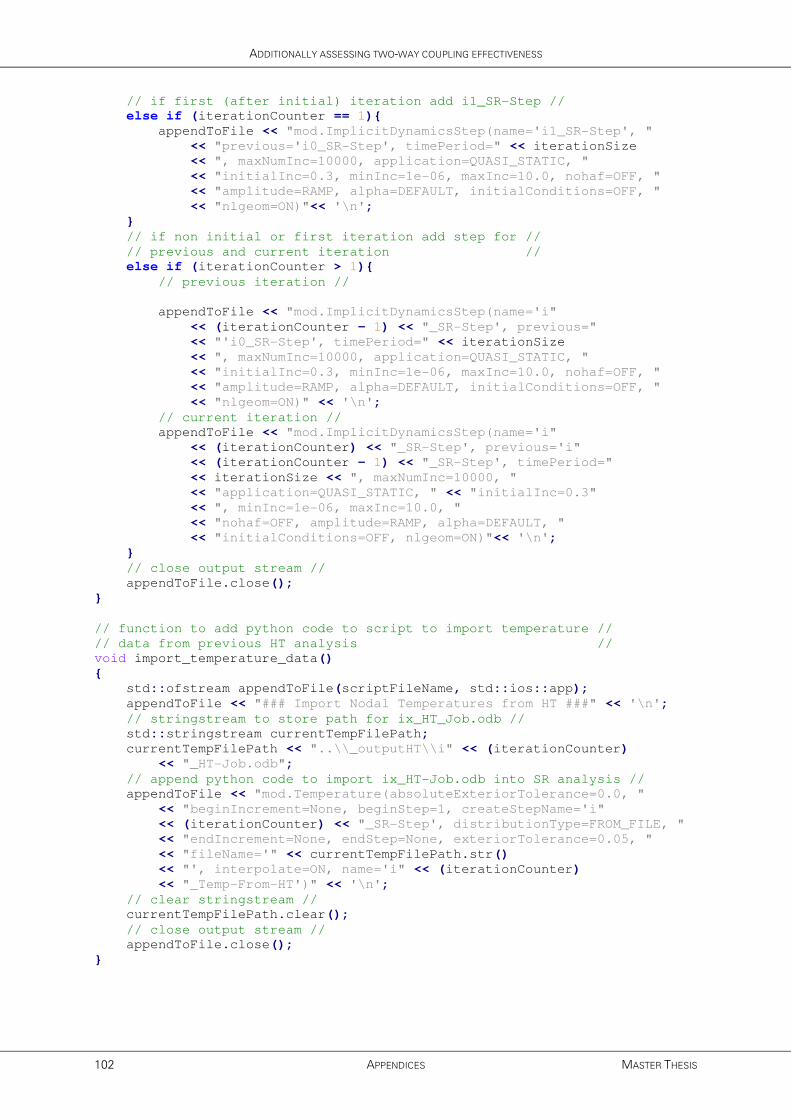
ADDITIONALLY ASSESSING TWO-WAY COUPLING EFFECTIVENESS
102 APPENDICES MASTER THESIS
// if first (after initial) iteration add i1_SR-Step //
else if (iterationCounter == 1){
appendToFile << "mod.ImplicitDynamicsStep(name='i1_SR-Step', "
<< "previous='i0_SR-Step', timePeriod=" << iterationSize
<< ", maxNumInc=10000, application=QUASI_STATIC, "
<< "initialInc=0.3, minInc=1e-06, maxInc=10.0, nohaf=OFF, "
<< "amplitude=RAMP, alpha=DEFAULT, initialConditions=OFF, "
<< "nlgeom=ON)"<< '\n';
}
// if non initial or first iteration add step for //
// previous and current iteration //
else if (iterationCounter > 1){
// previous iteration //
appendToFile << "mod.ImplicitDynamicsStep(name='i"
<< (iterationCounter - 1) << "_SR-Step', previous="
<< "'i0_SR-Step', timePeriod=" << iterationSize
<< ", maxNumInc=10000, application=QUASI_STATIC, "
<< "initialInc=0.3, minInc=1e-06, maxInc=10.0, nohaf=OFF, "
<< "amplitude=RAMP, alpha=DEFAULT, initialConditions=OFF, "
<< "nlgeom=ON)" << '\n';
// current iteration //
appendToFile << "mod.ImplicitDynamicsStep(name='i"
<< (iterationCounter) << "_SR-Step', previous='i"
<< (iterationCounter - 1) << "_SR-Step', timePeriod="
<< iterationSize << ", maxNumInc=10000, "
<< "application=QUASI_STATIC, " << "initialInc=0.3"
<< ", minInc=1e-06, maxInc=10.0, "
<< "nohaf=OFF, amplitude=RAMP, alpha=DEFAULT, "
<< "initialConditions=OFF, nlgeom=ON)"<< '\n';
}
// close output stream //
appendToFile.close();
}
// function to add python code to script to import temperature //
// data from previous HT analysis //
void import_temperature_data()
{
std::ofstream appendToFile(scriptFileName, std::ios::app);
appendToFile << "### Import Nodal Temperatures from HT ###" << '\n';
// stringstream to store path for ix_HT_Job.odb //
std::stringstream currentTempFilePath;
currentTempFilePath << "..\\_outputHT\\i" << (iterationCounter)
<< "_HT-Job.odb";
// append python code to import ix_HT-Job.odb into SR analysis //
appendToFile << "mod.Temperature(absoluteExteriorTolerance=0.0, "
<< "beginIncrement=None, beginStep=1, createStepName='i"
<< (iterationCounter) << "_SR-Step', distributionType=FROM_FILE, "
<< "endIncrement=None, endStep=None, exteriorTolerance=0.05, "
<< "fileName='" << currentTempFilePath.str()
<< "', interpolate=ON, name='i" << (iterationCounter)
<< "_Temp-From-HT')" << '\n';
// clear stringstream //
currentTempFilePath.clear();
// close output stream //
appendToFile.close();
}

FDS-2-ABAQUS: C++ MANAGED AUTOMATED PYTHON SCRIPTED CFD-FEM COUPLING
J.A. FEENSTRA APPENDICES 103
// function to append code to read the restart file from previous //
// iteration and request a new restart file for this iteration //
void append_restart_job_step()
{
// create output stream to SR_script.py //
std::ofstream appendToFile(scriptFileName, std::ios::app);
appendToFile << "### Define Restart Job/Step ###" << '\n';
// if non-zeroth iteration then append python code to read restart //
// file from previous iteration and request a new restart file //
// for this iteration //
if (iterationCounter > 0){
appendToFile << "mod.setValues(restartJob='i"
<< (iterationCounter - 1) << "_SR-Job', restartStep='i"
<< (iterationCounter - 1) << "_SR-Step')" << '\n';
appendToFile << "### Request Restart File for New Step ###"<< '\n';
appendToFile << "mod.steps['i" << iterationCounter
<< "_SR-Step'].Restart(frequency=0, numberIntervals=1, "
<< "overlay=ON, timeMarks=OFF)" << '\n';
}
// if zeroth iteration then no additional code is written //
// (only a comment) //
else if (iterationCounter == 0){
appendToFile << "#no additional restart information is written "
<< "since it is the initial (zero'th) iteration" << '\n';
}
// print error if iteration counter is negative //
// (should never occur) //
else if (iterationCounter < 0){
std::cerr << "Uh oh, iteration counter is negative check "
<< counterFileName << '\n';
exit(1);
}
// close output stream //
appendToFile.close();
}
// function to append instance (plate) (de)activation python code //
// for the current iteration //
void append_update_geometry()
{
// create output stream to SR_Script.py //
std::ofstream appendToFile(scriptFileName, std::ios::app);
// create input stream from plateLogFile //
std::ifstream plateLogFile(plateFailureFileName, std::ios::in);
// print error if plateLogFile can't be read/located //
if (!plateLogFile){
std::cerr << "Uh oh, plate failure log file "
<< plateFailureFileName
<< " could not be opened or does not exist!" << '\n';
exit(1);
}
appendToFile << "### Update Model Geometry ###" << '\n';
if (numberOfPlates == 1){
appendToFile << "# only a single plate in the model, "
<< "therefore no update is required" << '\n';
}
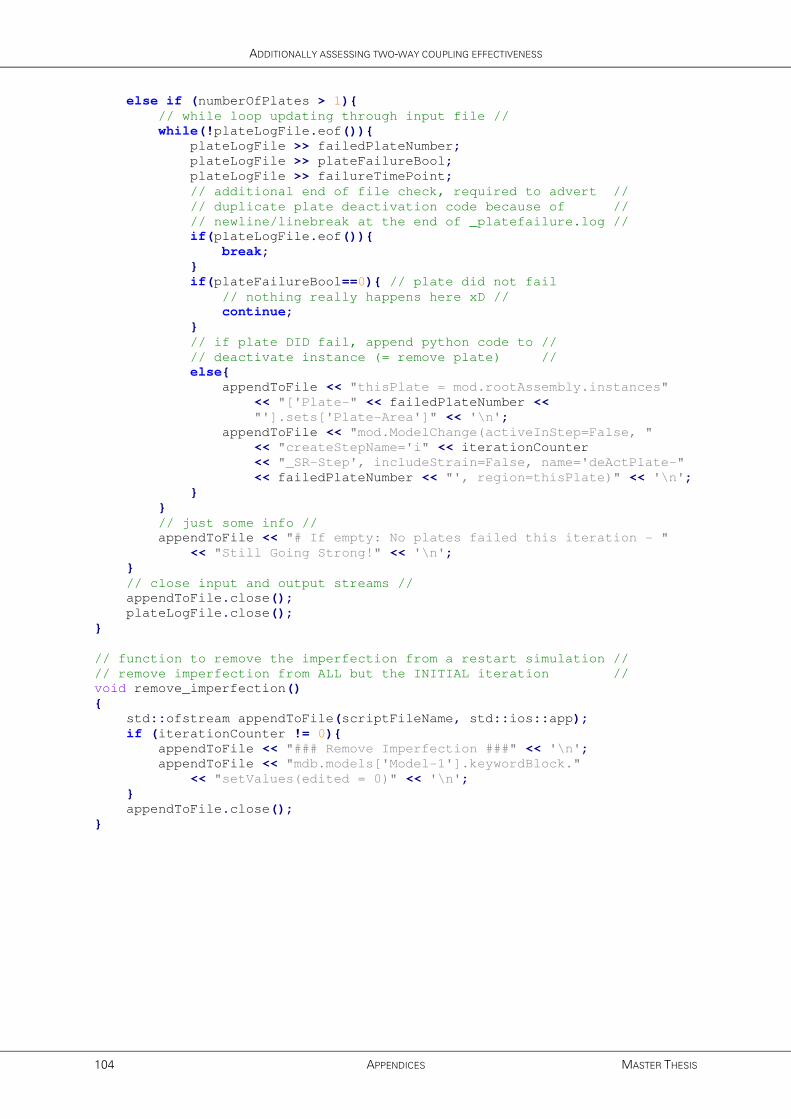
ADDITIONALLY ASSESSING TWO-WAY COUPLING EFFECTIVENESS
104 APPENDICES MASTER THESIS
else if (numberOfPlates > 1){
// while loop updating through input file //
while(!plateLogFile.eof()){
plateLogFile >> failedPlateNumber;
plateLogFile >> plateFailureBool;
plateLogFile >> failureTimePoint;
// additional end of file check, required to advert //
// duplicate plate deactivation code because of //
// newline/linebreak at the end of _platefailure.log //
if(plateLogFile.eof()){
break;
}
if(plateFailureBool==0){ // plate did not fail
// nothing really happens here xD //
continue;
}
// if plate DID fail, append python code to //
// deactivate instance (= remove plate) //
else{
appendToFile << "thisPlate = mod.rootAssembly.instances"
<< "['Plate-" << failedPlateNumber <<
"'].sets['Plate-Area']" << '\n';
appendToFile << "mod.ModelChange(activeInStep=False, "
<< "createStepName='i" << iterationCounter
<< "_SR-Step', includeStrain=False, name='deActPlate-"
<< failedPlateNumber << "', region=thisPlate)" << '\n';
}
}
// just some info //
appendToFile << "# If empty: No plates failed this iteration - "
<< "Still Going Strong!" << '\n';
}
// close input and output streams //
appendToFile.close();
plateLogFile.close();
}
// function to remove the imperfection from a restart simulation //
// remove imperfection from ALL but the INITIAL iteration //
void remove_imperfection()
{
std::ofstream appendToFile(scriptFileName, std::ios::app);
if (iterationCounter != 0){
appendToFile << "### Remove Imperfection ###" << '\n';
appendToFile << "mdb.models['Model-1'].keywordBlock."
<< "setValues(edited = 0)" << '\n';
}
appendToFile.close();
}

FDS-2-ABAQUS: C++ MANAGED AUTOMATED PYTHON SCRIPTED CFD-FEM COUPLING
J.A. FEENSTRA APPENDICES 105
// function appending python code to create and run (restart) job //
// 'normal' job for initial (zeroth) iteration, restart for other //
void append_create_and_run_job()
{
// create output stream to SR_Script.py //
std::ofstream appendToFile(scriptFileName, std::ios::app);
appendToFile << "### Create and Run Job ###" << '\n';
// if initial (zeroth) iteration append standard Job python code //
if (iterationCounter == 0){
appendToFile << "mdb.Job(name='i0_SR-Job', model='Model-1')"
<< '\n';
}
// if NON-initial iteration append restart Job python code //
else if (iterationCounter > 0){
appendToFile << "mdb.Job(name='i" << iterationCounter
<< "_SR-Job', model='Model-1', type=RESTART)" << '\n';
}
// append submit and run job python code to script //
appendToFile << "mdb.jobs['i" << iterationCounter
<< "_SR-Job'].submit(consistencyChecking=OFF)" << '\n';
appendToFile << "mdb.jobs['i" << iterationCounter
<< "_SR-Job'].waitForCompletion()" << '\n';
// append end of script line //
appendToFile << "############################## "
<< "End-Of-Script ##############################";
// close output stream //
appendToFile.close();
}
// function to backup SR_script for current iteration //
// rewriting script into file named ix_SR_script.py //
void create_backup_for_current_iteration()
{
// create input stream from SR_Script.py //
std::ifstream sourceFile(scriptFileName, std::ios::in);
// write backup filename to stringstream
backupFileName_ss.clear();
backupFileName_ss << "i" << iterationCounter << "_SR_Script.py";
// create output stream to SR_Script.py //
std::ofstream destFile(backupFileName_ss.str(), std::ios::out);
// print error if HT_Script.py can't be read/located //
if (!sourceFile){
std::cerr << "Uh oh, input file " << scriptFileName
<< " could not be opened or does not exist!" << '\n';
exit(1);
}
// rewrite content from buffer (input stream) to output stream //
else{
destFile << sourceFile.rdbuf() << '\n';
// close input and output streams //
sourceFile.close();
destFile.close();
}
}

ADDITIONALLY ASSESSING TWO-WAY COUPLING EFFECTIVENESS
106 APPENDICES MASTER THESIS
// function outputting (simple) completion message to console //
void process_completed()
{
std::cout << "[ [ [upGeomSR] ] ]" << '\n'
<< "Successfully updated SR python script for iteration: "
<< iterationCounter << '\n' << '\n';
}
int main()
{
read_current_iteration();
read_number_of_plates_and_partitions();
copy_basic_model_to_new_py();
append_new_step();
append_restart_job_step();
import_temperature_data();
append_update_geometry();
remove_imperfection();
append_create_and_run_job();
create_backup_for_current_iteration();
process_completed();
return 0;
}
/////////////////////////////// End of Code ///////////////////////////////
/////////////////////////////// upGeomSR ///////////////////////////////
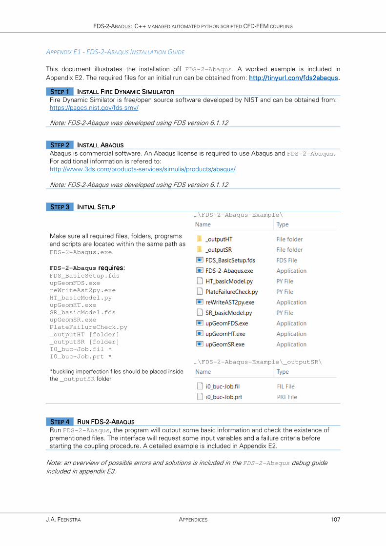
FDS-2-ABAQUS: C++ MANAGED AUTOMATED PYTHON SCRIPTED CFD-FEM COUPLING
J.A. FEENSTRA APPENDICES 107
APPENDIX E1 - FDS-2-ABAQUS INSTALLATION GUIDE
This document illustrates the installation off FDS-2-Abaqus. A worked example is included in
Appendix E2. The required files for an initial run can be obtained from: http://tinyurl.com/fds2abaqushttp://tinyurl.com/fds2abaqushttp://tinyurl.com/fds2abaqushttp://tinyurl.com/fds2abaqus....
SSSSTEP TEP TEP TEP 1111 IIIINSTALNSTALNSTALNSTALL L L L FFFFIRE IRE IRE IRE DDDDYNAMIC YNAMIC YNAMIC YNAMIC SSSSIMULATORIMULATORIMULATORIMULATOR
Fire Dynamic Similator is free/open source software developed by NIST and can be obtained from:
https://pages.nist.gov/fds-smv/
Note: FDS-2-Abaqus was developed using FDS version 6.1.12
SSSSTEP TEP TEP TEP 2222 IIIINSTALL NSTALL NSTALL NSTALL AAAABAQUSBAQUSBAQUSBAQUS
Abaqus is commercial software. An Abaqus license is required to use Abaqus and FDS-2-Abaqus.
For additional information is refered to:
http://www.3ds.com/products-services/simulia/products/abaqus/
Note: FDS-2-Abaqus was developed using FDS version 6.1.12
SSSSTEP TEP TEP TEP 3333 IIIINITIAL NITIAL NITIAL NITIAL SSSSETUPETUPETUPETUP
Make sure all required files, folders, programs
and scripts are located within the same path as
FDS-2-Abaqus.exe.
FDS-2-Abaqus requires:requires:requires:requires:
FDS_BasicSetup.fds
upGeomFDS.exe
reWriteAst2py.exe
HT_basicModel.py
upGeomHT.exe
SR_basicModel.fds
upGeomSR.exe
PlateFailureCheck.py
_outputHT [folder]
_outputSR [folder]
I0_buc-Job.fil *
I0_buc-Job.prt *
*buckling imperfection files should be placed inside
the _outputSR folder
…\FDS-2-Abaqus-Example\
…\FDS-2-Abaqus-Example\_outputSR\
SSSSTEP TEP TEP TEP 4444 RRRRUN UN UN UN FDSFDSFDSFDS----2222----AAAABAQUSBAQUSBAQUSBAQUS
Run FDS-2-Abaqus, the program will output some basic information and check the existence of
prementioned files. The interface will request some input variables and a failure criteria before
starting the coupling procedure. A detailed example is included in Appendix E2.
Note: an overview of possible errors and solutions is included in the FDS-2-Abaqus debug guide
included in appendix E3.

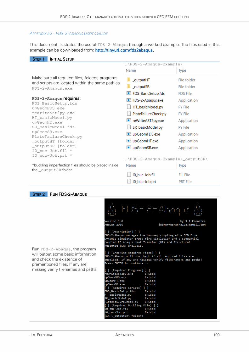
FDS-2-ABAQUS: C++ MANAGED AUTOMATED PYTHON SCRIPTED CFD-FEM COUPLING
J.A. FEENSTRA APPENDICES 109
APPENDIX E2 - FDS-2-ABAQUS USER’S GUIDE
This document illustrates the use of FDS-2-Abaqus through a worked example. The files used in this
example can be downloaded from: http://tinyurl.com/fds2abaqushttp://tinyurl.com/fds2abaqushttp://tinyurl.com/fds2abaqushttp://tinyurl.com/fds2abaqus....
SSSSTEP TEP TEP TEP 1111 IIIINITIAL NITIAL NITIAL NITIAL SSSSETUPETUPETUPETUP
Make sure all required files, folders, programs
and scripts are located within the same path as
FDS-2-Abaqus.exe.
FDS-2-Abaqus requires:requires:requires:requires:
FDS_BasicSetup.fds
upGeomFDS.exe
reWriteAst2py.exe
HT_basicModel.py
upGeomHT.exe
SR_basicModel.fds
upGeomSR.exe
PlateFailureCheck.py
_outputHT [folder]
_outputSR [folder]
I0_buc-Job.fil *
I0_buc-Job.prt *
*buckling imperfection files should be placed inside
the _outputSR folder
…\FDS-2-Abaqus-Example\
…\FDS-2-Abaqus-Example\_outputSR\
SSSSTEP TEP TEP TEP 2222 RRRRUN UN UN UN FDSFDSFDSFDS----2222----AAAABAQUSBAQUSBAQUSBAQUS
Run FDS-2-Abaqus, the program
will output some basic information
and check the existence of
prementioned files. If any are
missing verify filenames and paths.
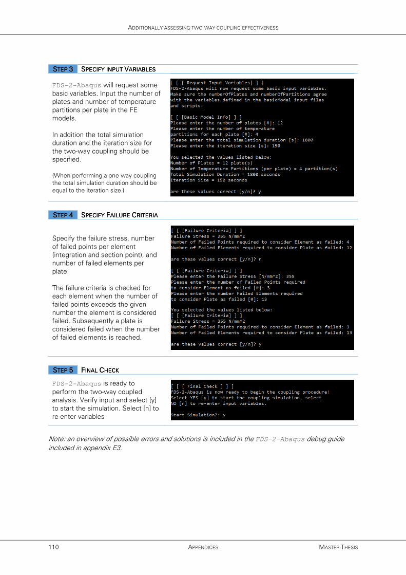
ADDITIONALLY ASSESSING TWO-WAY COUPLING EFFECTIVENESS
110 APPENDICES MASTER THESIS
SSSSTEP TEP TEP TEP 3333 SSSSPECIFY INPUT PECIFY INPUT PECIFY INPUT PECIFY INPUT VVVVARIABLESARIABLESARIABLESARIABLES
FDS-2-Abaqus will request some
basic variables. Input the number of
plates and number of temperature
partitions per plate in the FE
models.
In addition the total simulation
duration and the iteration size for
the two-way coupling should be
specified.
(When performing a one way coupling
the total simulation duration should be
equal to the iteration size.)
SSSSTEP TEP TEP TEP 4444 SSSSPECIFY PECIFY PECIFY PECIFY FFFFAILURE AILURE AILURE AILURE CCCCRITERIARITERIARITERIARITERIA
Specify the failure stress, number
of failed points per element
(integration and section point), and
number of failed elements per
plate.
The failure criteria is checked for
each element when the number of
failed points exceeds the given
number the element is considered
failed. Subsequently a plate is
considered failed when the number
of failed elements is reached.
SSSSTEP TEP TEP TEP 5555 FFFFINAL INAL INAL INAL CCCCHECKHECKHECKHECK
FDS-2-Abaqus is ready to
perform the two-way coupled
analysis. Verify input and select [y]
to start the simulation. Select [n] to
re-enter variables
Note: an overview of possible errors and solutions is included in the FDS-2-Abaqus debug guide
included in appendix E3.
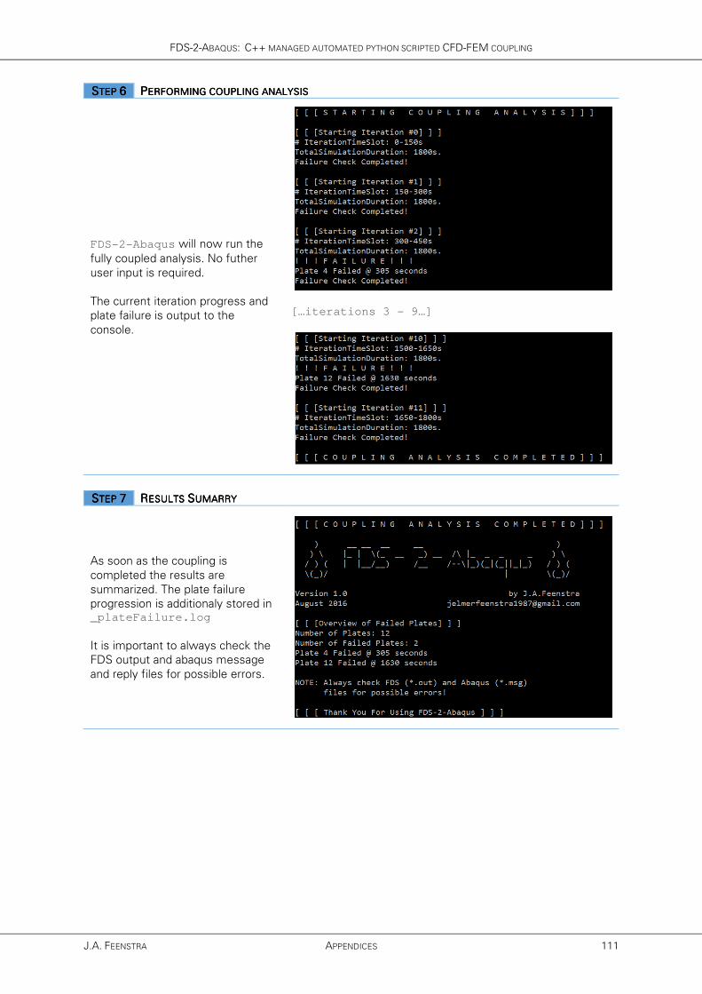
FDS-2-ABAQUS: C++ MANAGED AUTOMATED PYTHON SCRIPTED CFD-FEM COUPLING
J.A. FEENSTRA APPENDICES 111
SSSSTEP TEP TEP TEP 6666 PPPPERFORMING COUPLING AERFORMING COUPLING AERFORMING COUPLING AERFORMING COUPLING ANALYSISNALYSISNALYSISNALYSIS
FDS-2-Abaqus will now run the
fully coupled analysis. No futher
user input is required.
The current iteration progress and
plate failure is output to the
console.
[…iterations 3 - 9…]
SSSSTEP TEP TEP TEP 7777 RRRRESULTS ESULTS ESULTS ESULTS SSSSUMARRYUMARRYUMARRYUMARRY
As soon as the coupling is
completed the results are
summarized. The plate failure
progression is additionaly stored in _plateFailure.log
It is important to always check the
FDS output and abaqus message
and reply files for possible errors.

FDS-2-ABAQUS: C++ MANAGED AUTOMATED PYTHON SCRIPTED CFD-FEM COUPLING
J.A. FEENSTRA APPENDICES 113
APPENDIX E3 - FDS-2-ABAQUS DEBUG GUIDE
This docement gives a brief overview of possible challenges during a FDS-2-Abaqus managed two-
way coupled CFD-FEM analysis.
“FDS-2-Abaqus seems to run correctly but does not show the completion info”
� Due to its interdependency on the various scripts and programs a simple discontinuity (for
instance wrongly described paths) can result in crashing the complete program tree.
� Possible solution:
� Check the FDS output (*.out) and abaqus message (*.msg) and reply (*.rpy) files for
possible errors.
“FDS Fire modelling crashes – Numerical instability”
� Debug FDS model by running isloted FDS simulation.
� A possible reason for a Numerical Instability is the occurance of unrealistic velocities due to
sudden changes in HRR.
� Possible solution:
� Change HRR value
“FDS-2-Abaqus stuck in structural response simulation”
� Sometimes FDS-2-Abaqus gets stuck due to a convergence error. Possibly due to multiple
stable solution as a result of the various buckling modes.
� Possible solutions include:
� Change imperfection size.
� Change (FDS-2-Abaqus) iteration size.
� Change ‘Request fieldOutput interval’
“FDS-2-Abaqus stuck in PlateFailureCheck.py”
� The number of stress values in the output database increases quickly based on the number of
plates, the field output request interval, and the simulation duration. Patience is key.