The Impacts of Historical and Ongoing Human Activities on

Amphibian Diversity in Bilsa Biological Station,

Western Ecuador

by

Gregor F.M. Jongsma

Thesis submitted in partial fulfillment of the

requirements for the Degree of

Bachelor of Science with

Honours in Biology

Acadia University

2012

© Copyright by Gregor F.M. Jongsma 2012

ii

This thesis by Gregor F.M. Jongsma is accepted in its present form by the Department of

Biology as satisfying the thesis requirements for the degree of Bachelor of Science with

Honours.

Approved by the Thesis Supervisor

__________________________ ____________________

(Tom Herman) Date

Approved by the Head of the Department

__________________________ ____________________

(Soren Bondrup-Nielsen) Date

Approved by the Honours Committee

__________________________ ____________________

(Pritham Ranjan) Date

iii

I, Gregor F.M. Jongsma, grant permission to the University Librarian at Acadia University to

reproduce, loan or distribute copies of my thesis in microform, paper or electronic formats on a

non-profit basis. I, however, retain the copyright in my thesis.

_________________________________

Signature of Author

_________________________________

Date

iv

Acknowledgements

I am grateful for the assistance provided by staff of the Jatún Sacha Foundation and Bilsa

Biological Station, particularly C. Aulestia and J. Bermingham, and by field researchers D.

Caberera, L. Carrasco, F. Castillo, and J. Olivo. For assistance with species identification many

thanks go to G. Vigle and M. Ortego-Andrade. At Acadia, T. Herman and S. Bondrup-Nielsen

provided valuable input throughout the writing process of my thesis. Research was supported by

the National Science Foundation (OISE-0402137), National Geographic Society, Conservation,

Food and Health Foundation and Disney Wildlife Conservation Fund.

v

Table of Contents

List of Tables............................................................................................................vi

List of Figures ......................................................................................................... vii

Abstract .................................................................................................................. viii

Introduction ............................................................................................................... 1

Materials and Methods ............................................................................................... 5

Results ..................................................................................................................... 11

Discussion ............................................................................................................... 15

Literature Cited ........................................................................................................ 21

Appendix 1 ............................................................................................................................................ 24

Appendix 2..............................................................................................................25

Appendix 3......................................................................................................26

Appendix 4......................................................................................................30

vi

List of Tables

Table 1: Number of individual amphibians recorded across seven habitat categories in Bilsa

Biological Station, Ecuador.

Table 2: Total individuals, diversity (Shannon-Wiener and Simpson‘s respectively), observed

and expected species richness for the seven habitat categories.

vii

List of Figures

Figure 1: Three maps showing where Ecuador is located in South America, where the Mache

Chindul Reserve is located in Ecuador and where Bilsa (where the study was conducted) is

located within the Mache Chindul Reserve.

Figure 2: Expected species accumulation curves for amphibians captured in different habitat

categories in Bilsa Biological Station, according to the Mao Tau index. The vertical hatched line

indicates the minimum abundance level recorded for comparison across habitat types. Curves

were re-scaled to show accumulation of species in relation to number of captured individuals.

viii

Abstract

Human activity in western Ecuador is extensive in the form of logging and slash-and-

burn agriculture, however the impacts of these activities on amphibian diversity is almost

completely unknown. During a nine-month study in the Bilsa Biological Station situated in the

province of Esmeraldas, Ecuador I attempted to evaluate the impacts of these activities.

Amphibian diversity was estimated using visual encounter surveys along transects in pristine

sites (forest and river habitat that has no history of human activities) and historically disturbed

sites (forest and river habitat that was logged between 1989 and 1995) as well as along roads

with varying levels of ongoing human activity. The results of this study indicate that the

influence of disturbance on the diversity and composition of amphibian assemblages in the Bilsa

Biological Station varies with habitat. Amphibian assemblages along rivers were the richest as

well as the least impacted by human activity. Diversity and species richness were lower in

secondary than in primary forest suggesting that amphibian assemblages in interior forest habitat

are more vulnerable to disturbances caused by logging. Road habitat around Bilsa harboured a

very different amphibian assemblage from that of forest and river habitats. The results of this

study show that amphibian assemblages vary markedly in vulnerability to disturbances by human

activity; recognising these differences is critical for developing land management plans that

promote amphibian diversity in north western Ecuador.

1

Introduction

Evidence is mounting that humanity is driving a sixth mass extinction event that is notable

for its unprecedented rate of species loss (Wilson 1992). Amphibians—frogs, salamanders and

caecilians— are the oldest group of terrestrial vertebrates, and are currently facing risk of

extinction world-wide (Stuart 2004; Wake and Vredenburg 2008). Of the 6,800 known

amphibian species approximately one third are listed as threatened and at least 43% are in

decline (Collins et al. 2007). In the past three decades, the rate of amphibian extinction has

exceeded the mean extinction rate of the last 350 million years 200-fold (Roelants et al. 2007).

Amphibians are well suited as indicator species for assessing the health of ecosystems and

because they inhabit most of the world‘s fresh-water and terrestrial biomes, they may serve as

ideal indicators of global biological health and predictors for world-wide species extinctions

(Collins and Halliday 2005).

There are many factors causing amphibians to decline world-wide and the complex

interactions among these factors are poorly understood (Collins et al. 2007). The factors causing

the decline include: environmental contamination, invasive species, disease, climate change, and

deforestation (Stuart 2004). All of these factors result in the alteration of natural habitats and all

are linked to the activities of our ever-growing human population (Wake and Vredenburg 2008).

One of the most prominent forms of habitat alteration, the conversion of forests to agricultural

lands, plantations, and cattle ranches, is occurring at an alarming rate in the tropics. It would be

difficult to find a region in the tropics where this is more evident than in the Chocó

biogeographic region in north-western Ecuador.

Today, conservationists refer to the Chocó region as the Tumbes-Chocó-Magdalena

hotspot—an area covering 274,597 km², extending along the coast of Peru north through coastal

2

Ecuador and Columbia to southern Panama. The region has been coined the ―hottest‖ of

biodiversity hotspots, one demanding immediate international attention as a conservation priority

(Parker and Carr 1992; Mittermeier et al. 1998). Rampant deforestation set this region apart

from other hotspots around the world as less than two percent of the original forest cover remains

(Dodson and Gentry 1991). Even these remnant stands are under siege by a combination of

corporate operations (logging, cattle ranching, African palm and banana plantations) and the

activities of impoverished Ecuadorian farmers (slash and burn agriculture and poaching).

Threats

Logging has played the most pervasive role in transforming the Mache-Chindul— an area

of the Tumbes-Chocó-Magdalena in north coastal Ecuador— both directly and indirectly

(Hamilton et al. Unpublished). Clear-cutting and selective logging transform the landscape by

removing the trees; roads created in the process allow access to land that becomes occupied by

farmers whose activities further transform the area. Cattle pastures and banana and African palm

plantations, as well as small-scale subsistence farms, are prevalent in the region. These activities

inhibit forest regeneration and further deplete the already nutrient-poor soil. As a result, the

Mache-Chindul landscape is now a matrix of pasture-land dotted with patches of primary and

secondary forest— mostly on steep hillsides unfit for grazing cattle or growing crops. The

severe fragmentation of this forest landscape has many implications for amphibians and other

flora and fauna local to the Chocó.

Endemism

An endemic species is one that is restricted to a single locality (Hickman et al. 2008).

3

Coastal Ecuador harbours some of the highest levels of endemism on earth and amphibians in the

region are no exception. Of the 213 recognized amphibian species in the Tumbes-Chocó-

Magdalena, 40 are endemic (Conservation International). Endemic species are inherently at

greater threat of extinction due to their naturally restricted distributions (David 2005).

Most of the world‘s amphibians live in the tropics, where they occupy small geographic

ranges and have specific micro-habitat requirements (Wake and Vredenburg, 2008). These

characteristics leave amphibians vulnerable to rapid extinction. Some species, like the glass frog

Cochranella mache, have only been recorded along a few mountain streams in Western Ecuador

(IUCN). Human encroachment into this small area could very well eliminate the entire species.

Given the intensity of historical and current habitat alteration in the region, many species have

almost certainly perished undocumented and will likely continue to be lost. Habitat destruction

in regions with such high levels of endemism significantly reduces global biodiversity, and

conservation in these regions should be made an international priority.

Conservation

Successful species management and recovery require a number of steps. Amphibian

conservation in the Mache-Chindul is under-developed and a number of initiatives are still

required: (1) current amphibian diversity and population trends need to be accurately assessed,

(2) areas of high conservation priority (i.e. areas with high amphibian diversity or immediately

threatened by human activity) and corridors connecting them need to be identified and protected,

(3) suitable amphibian habitat needs to be allowed to regenerate (Young et al. 2001).

Unfortunately, reserves in Ecuador, as in most of the developing world, are poorly

protected. Illegal logging and slash and burn agriculture in the Mache Chindul are widespread

4

even within protected areas. If the three initiatives above are to be successful Ecuador‘s

government must provide adequate funding for reserves and hold corporations or individuals

who break the law accountable.

Equally important, government and NGOs must provide local residents with sustainable

economic alternatives that promote amphibian diversity, rather than degrade it. Any successful

amphibian conservation initiative will require the collaboration of scientists, government, NGOs,

and, above all, local people.

Objectives

The objectives of this study were two-fold. The first objective was to document the

species diversity of amphibians at Bilsa Biological Station. Over a nine month period amphibian

diversity was estimated using visual encounter surveys along transects in pristine and historically

disturbed forest sites as well as along roads with varying levels of human activity. Because

amphibians in this area are poorly known, these basic surveys contributed to the first complete

inventory of species composition and richness that is critical to any future conservation efforts.

The second objective was to gain insights into the influence of habitat on amphibian

diversity and abundance. To address this question, amphibians were sampled from a range of

habitats including forests, roadsides, and waterways. In this component of the study, I also

addressed how anthropogenic activity may be affecting amphibians by comparing each habitat

type (e.g., forest, road and river) in pristine conditions and in disturbed conditions.

5

Materials and Methods

Study Area

The Mache-Chindul mountain range of north-western Ecuador harbours some of the

greatest biodiversity on earth with a high degree of floral and faunal endemism. Two major

forest categories are found on this mountain range: (1) Humid Pre-Montane forest at elevations

between 500 and 1800 m, and (2) Humid Tropical rainforest below 500 meters. As part of the

Tumbes-Choco-Magdalena (TCM) biodiversity hotspot, international pressure to preserve the

region‘s unique ecosystems resulted in the creation of the Mache-Chindul Ecological Reserve

(MCER) in 1996

(http://www.ambiente.gov.ec/paginas_espanol/4ecuador/docs/areas/mache.htm). Based on the

author‘s personal observations little is being done to curb illegal logging, agriculture or poaching

and much of this 70,000 hectare area remains under threat. As a result, the park today is largely

deforested and consists mainly of small scale farms, cattle ranches, and African-palm

plantations, interspersed with small forest fragments. A smaller reserve inside the MCER, Bilsa

Biological Station, is privately owned and managed by the Jatun Sacha Foundation and is

sufficiently protected.

This study of amphibian diversity was carried out over nine months in 2007 in the Bilsa

Biological Station (79º 45‘ W, 0º 22‘ N, 330-730 meters above sea level) in the province of

Esmeraldas, Ecuador (Figure 1). The Tumbes-Choco-Magdalena region is one of the wettest

places on earth, and Bilsa receives on average more than 300 cm of rain per year. The

temperature is very stable. During the rainy season from January to June the average

temperature ranges between 24°C and 25°C. During the dry season from July to December the

average temperature is between 21°C and 22°C. With elevations ranging from 300m to 730m

6

Bilsa offers protection for both Humid-Pre-Montane forest and Humid Tropical forest. Being

one of the largest patches of remnant forest in North-Western Ecuador, Bilsa protects a mosaic of

primary and secondary forest covering an area of 3300 hectares, 80% of which is primary forest;

the remaining 20% of forest has been allowed to regenerate over the past 12-18 years. This

makes Bilsa one of the most representative areas in terms of existing or former diversity in the

surrounding valleys and rivers of the Mache-Chindul.

Selecting Sites

Rivers: River transect sites were selected based on the type of forest habitat surrounding

them (i.e. primary or secondary). Primary forest (never logged) and secondary forest (logged 12-

18 years previously) were identified with the help of experienced park staff. In addition to forest

habitat type, selection of sites required year-round water-flow and sufficient safety for

investigators to access and sample. Wherever possible, river sites with the most similar bank-

width and water velocity were selected; however, given the high heterogeneity of the area this

was not always possible. In all cases eight common environmental variables, described in detail

below, were recorded for each river transect. In total, 36 sampling sessions were conducted

across 18 river transects in primary forest habitat and 34 sampling sessions were conducted

across 17 transects in secondary forest habitat.

Interior Forest: Forest transect sites were selected in areas that had been characterized by

a team of ornithologists as either primary or secondary; this ensured sampling was conducted in

both forest habitat types equally (Appendix 1). Sixteen transects were set up within 6 primary

forest sites and sixteen transects were set up within 6 secondary forest sites. Transects ran

perpendicular and parallel to walking trails, at random distances within the sites identified by the

7

team of ornithologists. There were a total of 32 sampling sessions in primary forest and 32

sampling sessions in secondary forest.

Road: To investigate the influence of ongoing human disturbances three different road

categories were identified and sampled: (1) roads bordered by secondary forest on both sides (16

sample sessions along 8 transects), (2) roads with secondary forest on one side and pasture land

on the other (14 sample sessions along 7 transects), and (3) roads with pasture land on both sides

(17 sample sessions along 8 transects). The roads were unpaved and inaccessible by vehicles

approximately ten months of the year due to the muddy conditions.

Figure 1: Three maps showing where Ecuador is located in South America, where

the Mache Chindul Reserve is located in Ecuador and where Bilsa (where the study

was conducted) is located within the Mache Chindul Reserve.

Sampling Scheme

Amphibian sampling occurred from March to November 2007. For all habitats (rivers,

interior forest, roads), sampling was conducted using visual encounter surveys (VES) along

transects (Heyer et al. 1994). This involved walking slowly along 50 meter transects, intensively

searching with a stick through all leaf-litter and on all leaves and stems within transects for

amphibians. Transects in interior forest were 2m wide, while river transects were as wide as the

8

river-bank (1-3m) and road transects were as wide as the road-side (1-4m). Each transect was

laid-out at least two weeks prior to sampling to avoid any effects of disturbance. Each transect

was sampled twice: once in the morning and again at night. All amphibians encountered during

morning sampling sessions were captured and only released after the night sampling session was

complete. In addition to capturing individuals encountered during the morning sample session,

the location of each transect was changed each month. Employing this approach is a less

invasive way to avoid re-sampling individuals than toe-clipping, which many studies have shown

to negatively impact frogs (Davis and Ovaska 2001; McCarthy and Parris 2004; Waddle, et al.

2008). Changing the location of transects each month was also important to avoid modifying the

habitat along transects caused by repeated sampling in the same area. This is particularly an

issue in the tropics where the forest floor very readily turns to mud when disturbed.

Four river transects were sampled twice each month (two in secondary forest habitat; two

in primary forest habitat) for a total of 36 sampling sessions along rivers in primary forest and 34

along rivers in secondary forest (sampling along rivers in secondary forest was missed one

month due to health complications). River banks, defined as the area between the water and the

forest edge, were intensively searched for amphibians along both sides of the river for 50 m. All

leaves and branches overhanging the river banks (as high as 3.5 m) were also searched at each

river transect. Similarly, four interior forest transects were sampled twice each month (two in

primary forest; two in secondary) for a total of 18 transects in each habitat. For the forest

transects, two 50 m lengths of string were laid down in parallel rows two meters apart and all

leaf litter, logs, branches and leaves inside the two strings were searched for amphibians. Each

of the three road habitat categories was sampled twice each month.

9

Environmental Variables

For each transect, the weather conditions, number of people searching, and time spent

sampling were recorded. For each frog encountered, the species, age classification (adult,

adolescent, juvenile), and substrate were recorded during the sampling session. Depending on

the habitat, the appropriate environmental variables were recorded.

Environmental variables recorded along river transects included: bank-width, water-

width, water velocity, depth, understory density (1) over the bank and (2) over the water. All of

these variables were measured at 10 m intervals along each transect and then averaged. Water

velocity was measured by dropping a ping-pong ball in the river and timing how long it took to

travel one meter. Relative understory density was obtained by averaging the number of contacts

of vegetation (leaves and branches) with a 2 m tall stick placed vertically every 10 m along a

transect. This was measured at the edge of the forest and the edge of the water. The number of

waterfalls and pools was also recorded for each river transect. Leaf-litter depth and understory

density were measured at each forest transect at 10 m intervals and averaged. The road side

width, road wetness, type of vegetation and average vegetation height were recorded for each

road transect. Vegetation type was categorized as either grass or shrubs. Road wetness was

ranked on a scale of 0-5, with 0 being completely dry and 5 being more water than road.

Species Identification

During the first two months of amphibian sampling, all individuals encountered along

transects were captured and photographed for subsequent identification. Photographs were

shared with herpetologists in the US and Ecuador who had previous experience identifying

amphibians in the tropics. Dr. Greg Vigle has studied herpetofauna in Western Ecuador for the

10

past 25 years and carried out the first herpetological inventory of Bilsa in 2000. Dr. Vigle

provided help identifying amphibians encountered during this study via email. Marcelo Escobar

from the Natural History Museum in Quito has made numerous trips to Bilsa and is working to

create a complete herpetological inventory for the Mache-Chindul. Mr. Escobar offered

invaluable support in identifying the amphibians encountered over the course of this study. So,

although little work had been done on the assemblages of amphibians in altered versus pristine

forests in Bilsa, sufficient inventory work had been done in the park to identify the species

encountered during the course of this study with confidence.

Statistical Analysis

To examine how complete sampling was in different types of habitat and to compare species

richness across habitat types while controlling for differences in sample size, expected species

accumulation curves (also called ‗sample-based rarefaction curves‘, in which a sample is one sampling

occasion for a given station), were computed using the analytical formulas of Colwell et al. (2004) as

implemented in EstimateS v. 8 (Colwell 2006). Virtually any sampling methodology is imperfect in

completely detecting all the species present in a site, and several indices have been developed to estimate

―true‖ species richness based on sampling data (Colwell and Coddington 1994). As an estimation of the

total number of species present in each habitat category, the mean and range of four commonly employed

abundance-based estimators (ACE, Chao1, Jack1 and Boostrap), were calculated using EstimateS v. 8 and

based on 1,000 randomizations of samples without replacement. Two diversity indices were calculated

using EstimateS v. 8: Shannon-Wiener and Simpson`s. The Shannon-Wiener index places more weight on

rare species; conversely, Simpson`s index places less weight on rare species (Krebs 1999).

11

Results

Species Abundance and Diversity

In total 933 individuals were recorded: 613 along river and forest transects, and 320

along road transects (Table 1). Pristimantis achatinus dominated six of the seven habitat

categories and comprised more than half of the total of the individuals encountered during the

study. Hyloxalus awa was the most abundant species encountered along primary rivers and was

the second most abundant along secondary rivers.

12

Table 1: Number of individual amphibians recorded across seven habitat categories in

Bilsa Biological Station, Ecuador.

A sample-based rarefaction curve shows the accumulation curve of each habitat category

(Figure 2). In Bilsa Biological Station river habitat harboured the highest species richness

according to the Mau Tau index. Primary forest habitat harboured the third highest richness

levels, followed by the road habitat category, Pasture-Pasture. The latter two habitat categories

also had the steepest accumulation curves, which suggests that there are still more species to be

Forest River Road

Species Total 1° 2° 1° 2° Pasture 2° Mix

Bolitoglossa Spp. 1 0 0 0 1 0 0 0

Chaunus marinus 1 0 0 0 0 0 1 0

Caecilia leucocephala 1 0 0 1 0 0 0 0

Caecilia nigricans 1 0 0 0 0 1 0 0

Cochranella cf. albomaculata 4 0 0 2 2 0 0 0

C. Mache 2 0 0 2 0 0 0 0

C. Spinosa 1 0 0 1 0 0 0 0

Centrolene prosoblepon 37 0 0 23 14 0 0 0

Craugastor longirostris 8 1 2 2 2 1 0 0

Epipedobates boulengeri 27 1 0 16 10 0 0 0

Hyloxalus awa 114 0 0 79 35 0 0 0

H. sp. nov. 45 3 0 21 21 0 0 0

Hypsiboas pellucens 1 0 0 0 0 1 0 0

H. picturata 48 0 0 18 30 0 0 0

Leptodactylus labrosus 2 0 0 0 0 1 1 0

L. pentadactylus 1 1 0 0 0 0 0 0

Oophaga sylvatica 20 18 0 1 1 0 0 0

Pristimantis achatinus 535 50 97 45 39 91 114 99

P. parvillus 3 1 2 0 0 0 0 0

P.subsigillatus 2 0 0 0 0 1 0 1

P. walkeri 4 0 3 0 0 0 0 1

Rhinella margaritifer 37 0 0 9 28 0 0 0

Rhaebo haematiticus 31 0 0 19 12 0 0 0

Smilisca phaeota 7 0 0 0 0 1 3 3

Total 933 75 104 239 195 97 119 104

Primary habitat is represented by 1°, secondary habitat by 2°.

13

0

2

4

6

8

10

12

14

16

0 50 100 150 200 250 300

No. individuals

No

. s

pe

cie

s

River, Primary

River, Secondary

Forest, Primary

Forest, Secondary

Road, Secondary-Secondary

Road, Secondary-Pasture

Road, Pasture-Pasture

sampled in these habitats, particularly along roads surrounded by pasture. The remaining three

habitats had lower and similar richness levels.

Figure 2: Expected species accumulation curves for amphibians captured in different habitat

categories in Bilsa Biological Station, according to the Mao Tau index. The vertical hatched line

indicates the minimum abundance level recorded for comparison across habitat types. Curves were

re-scaled to show accumulation of species in relation to number of captured individuals.

Secondary river habitat had the highest diversity (Shannon-Wiener and Simpson‘s),

followed by primary river habitat (Table 2). Primary forest had higher amphibian diversity than

secondary forest. Road bordered by pasture had the highest diversity of the three road-categories.

The expected species richness (based on the mean of ACE, Chao1, Jack1, Bootstrap indices) was

most striking for the pasture-road habitat.

14

Table 2: Total individuals, diversity (Shannon-Wiener and Simpson’s respectively),

observed and expected species richness for the seven habitat categories.

Richness Diversity Total Ind.

Obs Expected Shan-W Simpson’s

Forest

Primary 7 13.1 (8.6-19.9) 0.9 2.0 75

Secondary 4 4.4 (4.0-5.0) 0.3 1.2 104

River Primary 14 17.2 (15.5-19.5) 2.0 5.7 239

Secondary 12 14.2 (13.0-15.5) 2.1 7.4 195

Road

Pasture 7 16.4 (9.1-22.0) 0.3 1.1 97

Secondary 4 5.8 (4.8-7.7) 0.2 1.1 119

Mix 4 5.8 (4.8-7.7) 0.2 1.1 104

Number of species observed (Obs), expected species richness (Expected) is the mean of four

common species richness indices (ACE, Chao1, Jack1, Bootstrap), Shannon-Wiener diversity index

(Shan-W), and Simpson‘s diversity index (Simpson‘s).

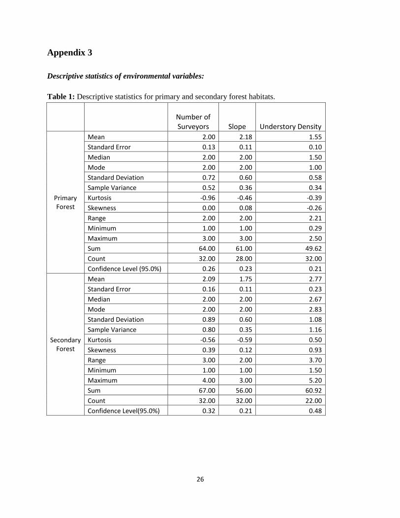
Environmental Variables

The mean understory density (USD) in primary forest (1.6) was much lower than the mean USD

of secondary forest (2.8) (Two sample t-test, p = 0.005). There was no significant difference

between any environmental variable in primary and secondary forest. Vegetation-height along

roads in pasture land was significantly lower than along roads in secondary forest or roads

bordered by pasture and secondary forest (One-way ANOVA, p = 0.052). No environmental

variable recorded had a significant correlation with diversity. Descriptive statistics (mean,

standard error, standard deviation, skewness, sample size) for each habitat category are included

in Appendix 3.

15

Discussion

Historical Disturbance

Throughout the tropics, alteration of forest habitat by logging and fragmentation

commonly results in reduced amphibian diversity and species richness (Pearman 1997;

Krishnamurthy 2003; Walting and Donnelly 2008). The results from this study show that the

influence of disturbance on the diversity and composition of amphibian assemblages in the

Mache-Chindul varies with habitat. Amphibian assemblages along rivers were the most diverse

as well as the least impacted by human activity in the form of logging 12-18 years prior to this

study. Diversity and species richness were lower in secondary than in primary forest suggesting

that amphibian assemblages in interior forest habitat are more vulnerable to disturbances caused

by logging.

Avian diversity sampled at the same forest sites in Bilsa exhibited the reverse response

and had higher diversity in secondary forest than in primary forest (Karubian unpublished). This

demonstrates how different groups of animals can respond very differently to disturbance and

suggests that amphibians in the Mache-Chindul are more negatively impacted by human

activities, like logging, than birds, in terms of overall diversity and species richness. All forest

sites in this study were part of a mosaic of habitat with direct contact zones between primary and

secondary forest. This type of setting makes it possible for amphibian populations in primary

forest to serve as a source in repopulating secondary forest following a major disturbance like

logging. Despite this, there was still a significant difference in diversity between primary and

secondary forest. What is more alarming about the apparent vulnerability of interior-forest

amphibian assemblages is that one could expect to find even lower amphibian diversity in

isolated secondary forests lacking available source populations.

16

The different responses between forest and river habitats may be explained by regular

disturbances along river-banks caused by rising water-levels during the wet season. This natural

disturbance results in a similar forest structure growing along both primary and secondary rivers.

This was demonstrated by the identical understory densities (USD) in both secondary and

primary river habitat. Conversely, mean understory densities differed greatly between primary

and secondary forest. Amphibian diversity richness is influenced by a number of environmental

variables (canopy cover, soil moisture, distance to nearest stream, invertebrate density) (Urbina-

Cardona et al. 2006). Recording more of these variables during this study may have helped

identify necessary microhabitat characteristics that support greater amphibian diversity or

richness at Bilsa.

Ongoing Disturbance

Road habitat around Bilsa harboured a very different amphibian assemblage from that of

forest and river habitats and of the nine species encountered along roads six were found in no

other habitats. Typically, amphibian assemblages in pasture land have lower diversity and

species richness (Tocher 1996; Pearman 1997, Urbina-Cardona et al. 2006) but roads in pasture

land surrounding Bilsa actually harbour the greatest species richness of the three road-categories.

Road wetness was similar across all road categories; however, vegetation height was

significantly shorter in pasture-road habitat. It is possible that species went undetected in

secondary-road and mixed-road habitats, despite rigorous sampling efforts.

Continued sampling in this habitat is needed to more accurately determine the actual

diversity and species richness. Additional sampling should be done in pasture away from roads

to determine whether the species encountered during this study are restricted to roads or are

widespread throughout pasture lands. This information, in combination with pasture diversity in

17

relation to distance from forest edge, will help gauge the overall amphibian diversity in the

Mache-Chindul as more and more forests are converted to pasture.

Amphibian Detection

Species detectability as defined by Boulinier et al (1998) is the probability of detecting at least

one individual of a given species in a particular sampling effort, given that individuals of that

species are present in the area of interest during the sampling session. This is a crucial factor to

consider for any study involving species richness or diversity estimates. Naturally, not all

species are equally detectable. Additionally, not all species are equally detectable across

different habitats. Fortunately, some species richness estimators take detectability into account.

Abundance-based Coverage Estimator (ACE) for example, separates common and rare species

from a sample and uses the rare subset to predict how many species are likely missing due to

lowered detectability (Chazdon 1998). The issue surrounding detectability is highlighted by

canopy dwelling species in the tropics.

Canopy dwelling species deserve more consideration when assessing amphibian diversity

in the tropics. Utilizing bromeliads as high-rise nurseries, some species may never have to

descend from the canopy and thus would never have been encountered in this study.

Consequently the true amphibian diversity of the forest may be under-estimated. Two species in

Bilsa exemplify the real possibility that amphibian assemblages, particularly frogs, could occupy

the canopy without ever descending.

Cochranella albomaculata, has only been encountered four times in Bilsa and each

encounter was of a mating-pair on a leaf overhanging a river (1-2 m above the water). C.

albomaculata is commonly encountered low on vegetation along rivers in Central America

18

(Savage 2002). Guayasamin (2007) proposed that what is currently identified as C.

albomaculata may actually be several species, as individuals from Columbia and Ecuador

exhibit larger spots on the dorsum than in Central America. These isolated encounters in Bilsa

support the possibility that C. albomaculata represents different species in Ecuador and, in Bilsa

at least, appear to have taken to the canopy, only returning to lower strata of the forest to

procreate. Only during mating was it possible to account for this species and it is likely that

many individuals were not recorded because they were too high in the canopy.

Oophaga sylvatica, is a ground-dwelling frog that uses the water trapped in bromeliads

for rearing its tadpoles. Secondary forest supports far fewer epiphytes than primary forest

(Turner 1997) which may explain why O. sylvatica was never encountered in secondary forest

during this study.

The combination of O. sylvatica‘s use of bromeliads and C. albomaculata‘s canopy-

dwelling life-style demonstrates that amphibian assemblages may exist undetected in the canopy

of primary forest, or in forest where sufficient epiphyte growth has occurred. As such, efforts to

detect canopy-dwelling amphibians should be undertaken more often when assessing diversity in

the tropical forests. This theory is supported by the discovery of Ecnomiohyla phantasmagoria

in Bilsa in 2009 (Patricio M. Olmedo, unpublished. See photograph in Appendix 4). E.

phantasmagoria is a canopy-dwelling species and it is likely that is was never detected during

this study or any previous ones, because of this. New developments in bioacoustics recording

devices may be the best solution to surveying amphibians in the canopy.

Amphibians as Indicator Species

At Jatun Sacha Biological Station in Amazonian Ecuador, Pearman (1997) found that

19

species richness of the genus Pristimantis declined with proximity to pasture and suggested that

Pristimantis may be a useful indicator assemblage for assessing the quality of Tropical Wet

Forest. The Pristimantis spp. at Bilsa Biological Station, however, exhibit the greatest richness

in pasture and secondary forest habitat. All Pristimantis species encountered in and around Bilsa

but one (P. achatinus) were very rare. These findings suggest that Prismantis has little value as

an indicator assemblage for assessing the quality of Pre-Montane or Humid Tropical Forest in

the Mache-Chindul.

Four species (Cochranella mache, C. spinosa, Caecilia leucocephala, and Leptodactylus

pentadactylus) encountered during this study were found exclusively in pristine habitat (primary

forest or river). All of these species were only encountered once or twice over the course of nine

months, thus making them poor indicator species. Oophaga sylvatica, however was encountered

18 times in pristine habitat and never in secondary forest habitat and may be a good candidate for

an indicator of pristine forest habitat in the Mache-Chindul since it (1) was the most abundant

amphibian found solely in pristine forest during this study, (2) is easily identified, (3) vocal

during the day and (4) is wide-spread in the region. All of these traits make its detection easy

and feasible. Surveys for the presence of O. sylvatica, in other pristine (and disturbed) forest

habitat across its range in the Tumbes-Chocó-Magdalena are needed before adopting this species

as a suitable indicator of quality pristine forest habitat.

Conservation Implications

The results of this study in Bilsa Biological Station show that amphibian assemblages

vary markedly in their vulnerability to disturbances by human activity. Recognising these

differences is critical for developing land management plans that promote amphibian diversity in

20

north western Ecuador.

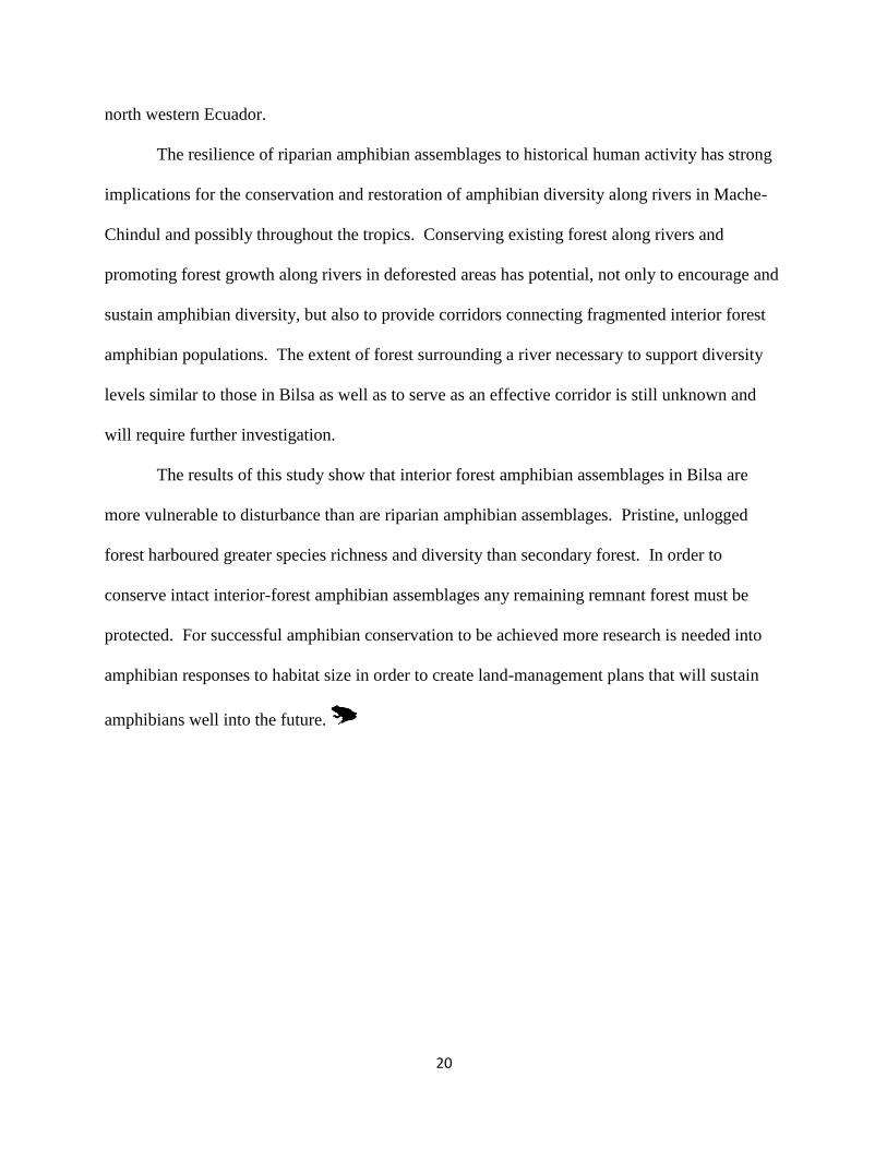
The resilience of riparian amphibian assemblages to historical human activity has strong

implications for the conservation and restoration of amphibian diversity along rivers in Mache-

Chindul and possibly throughout the tropics. Conserving existing forest along rivers and

promoting forest growth along rivers in deforested areas has potential, not only to encourage and

sustain amphibian diversity, but also to provide corridors connecting fragmented interior forest

amphibian populations. The extent of forest surrounding a river necessary to support diversity

levels similar to those in Bilsa as well as to serve as an effective corridor is still unknown and

will require further investigation.

The results of this study show that interior forest amphibian assemblages in Bilsa are

more vulnerable to disturbance than are riparian amphibian assemblages. Pristine, unlogged

forest harboured greater species richness and diversity than secondary forest. In order to

conserve intact interior-forest amphibian assemblages any remaining remnant forest must be

protected. For successful amphibian conservation to be achieved more research is needed into

amphibian responses to habitat size in order to create land-management plans that will sustain

amphibians well into the future.

21

Literature Cited

Bouliner, T., J. D. Nichols, J. R. Sauer, J. E. Hines, K. H. Pollock. 2005 Estimating species

richness : the importance of heterogeneity in species detectability. Ecology 79:1018-1028.

Chazdon, R. L., R. K. Colwell, J. S. Denslow, & M. R. Guariguata. 1998. Statistical methods for

estimating species richness of woody regeneration in primary and secondary rain forests of NE

Costa Rica. Parthenon Publishing, Paris.

Collins, J. P., C. Gascon, J.R. Medelson III. 2007. Amphibian Action Conservation Plan.

Preceedings of the IUCN/SSC Amphibian Conservation Summit in 2005.

Collins, J. P., T. Halliday. 2005. Forecasting changes in amphibian biodiversity: aiming at a

moving target. Philosophical Transactions of the Royal Society of London 360:309-214.

Colwell R.K., AND Coddington J.A. (1994) Estimating terrestrial biodiversity through

extrapolation. Philosophical Transactions of the Royal Society of London 345:101-118.

Colwell R.K., Mao C.X. & Chang J. (2004) Interpolating, extrapolating, and comparing

incidence-based species accumulation curves. Ecology 85:2717-2727.

Colwell, R. K. 2006. EstimateS: Statistical estimation of species richness and shared species

from samples. Version 8. Persistent URL <purl.oclc.org/estimates>

Conservation International. http://web.biodiversityhotspots.org/xp/Hotspots/tumbes_choco/bio

diversity.xml). Access date: 18 January 2009.

Davis, T. M., K. Ovaska. 2001. Individual Recognition of Amphibians: Effects of Toe Clipping and

Fluorescent Tagging on the Salamander Plethodon vehiculum. Journal of Herpetology 35:217-225.

Dodson, C. H., and A.H. Gentry. 1991. Biological extinction in western Ecuador. Annals of the

Missouri Botanical Garden 78:273-295.

Hamilton, P., C. Mouette, A. Almendariz. Initial analysis of coastal Ecuadorian herpetofauna of

dry and moist forests. Reptile and Amphibian Ecology International. Unpublished.

Hickman, C. P., L. S. Roberts, A. Larson, H. I'Anson. 2008. Integrated Principles of Zoology.

Fourteenth edition. McGraw-Hill Publishing Co., New York.

Heyer, W.R, M. A. Donnelly, R. W. McDiarmid, L. C. Hayek, M. S. Foster. 1994. Measuring

and Monitoring Biological Diversity: Standard Methods for Amphibians. First Edition.

Smithsonian.

Krebs, C. J. 1999. Ecological Methodology. Second Edition. Benjamin Cummings, New York.

22

McCarthy, M. A., K. M. Parris. 2004. Clarifying the effect of toe clipping on frogs with

Bayesian statistics. Journal of Applied Ecology 41:780-786.

Mittermeier, R. A., N. Myers, J. B. Thomsen, G. A. B. da Fonseca, S. Olivieri. 1998.

Biodiversity hotspots and major tropical wilderness areas: approaches to setting conservation

priorities. Conservation Biology 12:516-520.

Parker III, T.A., and J. L. Carr. 1992. Status of forest remnants in the Cordillera de la Costa and

adjacent areas of southwestern Ecuador. Conservation International RAP Working Papers 2:172.

Pearman, P.B. 1997. Correlates of amphibian diversity in an altered landscape of Amazonian

Ecuador. Conservation Biology 11:1211-1225.

Roelants, K., S. J. Gower, M. Wilkinson, S. P. Loader, S. D. Biju, K. Guillaume, L. Moriau, F.

Bossuyt. 2007. Global patterns of diversification in the history of modern amphibians.

Proceedings of the National Academy of Science 104:887-892.

Savage, M. J. 2002. The amphibians and reptiles of Costa Rica: a herpetofauna between two

continents, between two seas. University of Chicago Press.

Tocher, D. M. 1996. The effects of deforestation and forest fragmentation on a central

Amazonian frog community. University of Canterbury Press.

Turner, I.A., Y. K. Wong, P. T. Chew, A. Bin Ibrahim. 1997. Tree species richness in primary

and old secondary tropical forest in Singapore. Biodiversity and conservation 6:537-543.

Urbina-Cardona, J. N., M. Olivares-Pe´rez, V. H. Reynoso. 2005. Herpetofauna diversity and

microenvironment correlates across a pasture–edge–interior ecotone in tropical rainforest

fragments in the Los Tuxtlas Biosphere Reserve of Veracruz, Mexico. Biological Conservation

132:61-75.

Waddle, J. H., K. G. Rice, F. J. Mazzotti, H. F. Percival. 2008. Modeling the effect of toe

clipping on treefrog survival: beyond the return rate. Journal of Herpetology 42:467-473.

Wake, D. B., and V. T. Vredenburg. 2008. Are we in the midst of the sixth mass extinction? A

view from the world of amphibians. Proceedings of the National Academy of Science

105:11466-11473.

Watling, J. I., M. A. Donnelly. 2008. Species richness and composition of amphibians and

reptiles in a fragmented forest landscape in northeastern Bolivia. Basic and Applied Ecology

9:523–532.

Wilson, O. E., 1992. The Diversity of Life. W. W. Norton & Company. New York.

Young, B. E., K. R. Lips, J. K. Reaser, R. Ibanez, A. W. Salas, J. R. Cedeno, L. A. Coloma, S.

Ron, E. L. Marca, J.R. Meyer, A. Munoz, F. Bolanos, G. Chaves, D. Romo. 2001. Population

23

declines and priorities for amphibian conservation in Latin America. Conservation Biology

15:1213-1223.

24

Appendix 1

Quoted from Jordan Karubian’s methods (unpublished):

Forest type characterization

Along >15 km of trails that cover about a third of the Bilsa Station area, we establish sampling

points every 200 m (total: 84 points) where we visually classified the forest type around it as

primary (48 points), altered (16 points), or secondary (20 points, Fig. 1). To confirm if our visual

classification reflected actual differences in habitat structure, in each of these points we recorded:

the number of trees with DBH >10 but < 50 cm (within a 10 m-radius circle), number of trees

with DBH ≥ 50 cm (within a 20 m-radius circle), canopy height (in meters), amount of light

reaching the understory (measured with a densiometer, average of four measures), and elevation

(in meters). We then used a Discriminant Analysis (DA) to assess if sites could be confidently

assigned to forest type categories based on these structural variables.

25

Appendix 2

Table 1: Species richness results, calculated using Estimate S program: ACE, Chao 1, Jack 1 and

Bootstrap.

Habitat River Forest Road

Category Primary Secondary Primary Secondary Pasture Forest Mix

Samples 36 34 32 32 17 16 14

Individuals (computed) 239 195 75 104 97 119 104

Sobs (Mao Tau) 14 12 7 4 7 4 4

Sobs 95% CI Lower Bound 10.58 8.49 3.24 3.06 2.76 1.79 1.79

Sobs 95% CI Upper Bound 17.42 15.51 10.76 4.94 11.24 6.21 6.21

Sobs SD (Mao Tau) 1.74 1.79 1.92 0.48 2.16 1.13 1.13

Sobs Mean (runs) 14 12 7 4 7 4 4

ACE Mean 19.51 15.54 19.89 4 22 7.67 7.67

ACE SD (runs) 0 0

0 0

Chao 1 Mean 15.5 13 13 4 22 5 5

Chao 1 95% CI Lower Bound 14.17 12.09 7.96 4 10.32 4.08 4.08

Chao 1 95% CI Upper Bound 26.89 23.06 44.4 4 74.78 17.27 17.27

Chao 1 SD (analytical) 2.29 1.87 7.08 0 13.48 2.17 2.17

Jack 1 Mean 17.89 14.91 10.88 4.97 12.65 5.88 5.86

Jack 1 SD (analytical) 1.86 1.63 1.84 0.97 3.34 1.28 1.26

Bootstrap Mean 15.74 13.24 8.58 4.62 9.14 4.83 4.82

Bootstrap SD (runs) 0

0

0

26

Appendix 3

Descriptive statistics of environmental variables:

Table 1: Descriptive statistics for primary and secondary forest habitats.

Number of Surveyors Slope Understory Density

Primary Forest

Mean 2.00 2.18 1.55

Standard Error 0.13 0.11 0.10

Median 2.00 2.00 1.50

Mode 2.00 2.00 1.00

Standard Deviation 0.72 0.60 0.58

Sample Variance 0.52 0.36 0.34

Kurtosis -0.96 -0.46 -0.39

Skewness 0.00 0.08 -0.26

Range 2.00 2.00 2.21

Minimum 1.00 1.00 0.29

Maximum 3.00 3.00 2.50

Sum 64.00 61.00 49.62

Count 32.00 28.00 32.00

Confidence Level (95.0%) 0.26 0.23 0.21

Secondary Forest

Mean 2.09 1.75 2.77

Standard Error 0.16 0.11 0.23

Median 2.00 2.00 2.67

Mode 2.00 2.00 2.83

Standard Deviation 0.89 0.60 1.08

Sample Variance 0.80 0.35 1.16

Kurtosis -0.56 -0.59 0.50

Skewness 0.39 0.12 0.93

Range 3.00 2.00 3.70

Minimum 1.00 1.00 1.50

Maximum 4.00 3.00 5.20

Sum 67.00 56.00 60.92

Count 32.00 32.00 22.00

Confidence Level(95.0%) 0.32 0.21 0.48

27

Table 2: Descriptive statistics for primary and secondary river habitats.

Surveyors

(#) Slope USD

Forest USD

water Width Bank

Width Water Pool

Waterfalls

Depth Avg (cm)

Velocity

1 River

Mean 2.47 2.72 2.91 1.28 4.63 2.51 2.39 1.39 24.95 0.19

Standard Error 0.22 0.10 0.13 0.13 0.23 0.11 0.35 0.17 2.65 0.02

Standard Deviation 1.34 0.59 0.75 0.78 1.07 0.68 2.09 1.02 15.87 0.12

Sample Variance 1.80 0.35 0.56 0.61 1.15 0.47 4.36 1.04 251.99 0.01

Kurtosis 3.60 0.32 -0.78 0.48 -0.31 0.24 -

1.17 -1.21 -0.93 5.04

Skewness 1.68 0.80 0.27 0.87 -0.90 0.57 0.45 -0.19 0.73 2.24

Range 6.00 2.00 2.62 2.75 3.40 2.62 6.00 3.00 46.20 0.50

Minimum 1.00 2.00 1.58 0.25 2.40 1.54 0.00 0.00 6.80 0.09

Maximum 7.00 4.00 4.20 3.00 5.80 4.16 6.00 3.00 53.00 0.59

Sum 89.00 98.00 104.8

8 46.22 101.9

4 90.26 86.0

0 50.00 898.20 6.92

Count 36.00 36.00 36.00 36.00 22.00 36.00 36.0

0 36.00 36.00 36.00

Confidence Level(95.0%) 0.45 0.20 0.25 0.26 0.47 0.23 0.71 0.35 5.37 0.04

Mean 2.06 2.50 2.92 1.35 4.28 1.65 1.65 0.18 15.72 0.18

2 River

Standard Error 0.20 0.07 0.15 0.13 0.32 0.11 0.33 0.07 1.95 0.01

Standard Deviation 1.15 0.39 0.88 0.77 1.51 0.66 1.91 0.39 11.35 0.06

Sample Variance 1.33 0.15 0.77 0.60 2.27 0.44 3.63 0.15 128.77 0.00

Kurtosis 3.85 1.06 -0.77 -1.16 1.28 -0.16 -

1.20 1.23 -0.66 -0.01

Skewness 1.77 0.82 0.11 0.35 1.13 0.38 0.65 1.78 0.87 0.88

Range 5.00 1.50 3.00 2.34 5.58 2.53 5.00 1.00 34.80 0.22

Minimum 1.00 2.00 1.42 0.33 2.30 0.61 0.00 0.00 3.50 0.09

Maximum 6.00 3.50 4.42 2.67 7.88 3.14 5.00 1.00 38.30 0.31

Sum 70.00 85.00 99.26 45.82 94.08 56.22 56.0

0 6.00 534.34 6.04

Count 34.00 34.00 34.00 34.00 22.00 34.00 34.0

0 34.00 34.00 34.00

Confidence Level(95.0%) 0.40 0.14 0.31 0.27 0.67 0.23 0.66 0.14 3.96 0.02

28

Table 3: Descriptive statistics for pasture, forest and mixed road habitats.

Surveyors (#) Slope Mud

Veg. Height

Road Side

Width

Pasture

Mean 2.59 1.17 2.00 41.62 353.33

Standard Error 0.32 0.17 0.35 14.10 30.26

Median 2.00 1.00 2.00 20.00 450.00

Mode 2.00 1.00 1.50 20.00 450.00

Standard Deviation 1.33 0.41 1.26 50.83 117.21

Sample Variance 1.76 0.17 1.58 2583.26 13738.10

Kurtosis 1.86 6.00 -0.28 2.97 -1.03

Skewness 1.43 2.45 0.07 2.09 -0.71

Range 5.00 1.00 4.00 142.00 300.00

Minimum 1.00 1.00 0.00 13.00 150.00

Maximum 6.00 2.00 4.00 155.00 450.00

Sum 44.00 7.00 26.00 541.00 5300.00

Count 17.00 6.00 13.00 13.00 15.00

Confidence Level(95.0%) 0.68 0.43 0.76 30.71 64.91

Pasture, Forest

Mean 2.14 1.42 2.00 49.40 314.29

Standard Error 0.25 0.14 0.41 12.86 12.21

Median 2.00 1.25 1.75 35.00 350.00

Mode 2.00 1.00 2.00 30.00 350.00

Standard Deviation 0.95 0.47 1.31 40.65 45.69

Sample Variance 0.90 0.22 1.72 1652.71 2087.91

Kurtosis -0.69 -1.93 -0.58 1.09 -1.56

Skewness 0.31 0.38 0.41 1.60 -0.66

Range 3.00 1.00 4.00 108.00 100.00

Minimum 1.00 1.00 0.00 17.00 250.00

Maximum 4.00 2.00 4.00 125.00 350.00

Sum 30.00 17.00 20.00 494.00 4400.00

Count 14.00 12.00 10.00 10.00 14.00

Confidence Level(95.0%) 0.55 0.30 0.94 29.08 26.38

Forest

Mean 2.21 1.22 1.50 55.89 170.77

Standard Error 0.24 0.15 0.22 13.67 29.04

Median 2.00 1.00 2.00 40.00 125.00

Mode 2.00 1.00 2.00 30.00 125.00

Standard Deviation 0.89 0.44 0.71 41.00 104.70

Sample Variance 0.80 0.19 0.50 1680.86 10961.86

Kurtosis 1.00 0.73 0.57 -0.49 2.51

Skewness 1.04 1.62 -1.18 0.76 1.95

29

Range 3.00 1.00 2.00 117.00 300.00

Minimum 1.00 1.00 0.00 3.00 100.00

Maximum 4.00 2.00 2.00 120.00 400.00

Sum 31.00 11.00 15.00 503.00 2220.00

Count 14.00 9.00 10.00 9.00 13.00

Confidence Level(95.0%) 0.52 0.34 0.51 31.51 63.27

30

Appendix 4