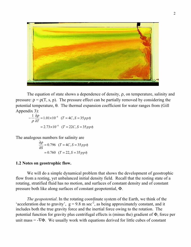
1

GFD – 2 Spring 2010 P.B. Rhines Lecture 1 with corrections 1.1 Properties of the ocean-climate system. Three dominant properties of both the atmosphere and ocean fluids are their thinness, stable layering, and planetary rotation. Typical winds have lateral scale ~ 3000 km, and vertical scale ~ 3 km, giving a 1:1000 aspect ratio. Ocean currents divide between boundary currents and eddies with L ~ 100 km and ocean-filling gyres with scale ~ 3000 km. Their vertical scale is about 300m, giving aspect ratios ranging between 1:10,000 to 1:300. As if that were not enough, the fluids are layered with stable density stratification, further inhibiting vertical velocity. The biology of the oceans is largely shaped by this layering. Upwelling of nutrient-rich deep waters to the thin upper layer reached by the sun has to fight against this stratification and is very difficult to achieve. A simple laboratory experiment shows the interleaving of layers of different density created by heating or cooling at the ocean surface. Starting from a homogenously constant density ocean, a simple, uniform cooling of the upper surface will drive only small-scale convection cells, whose width is about the same as the fluid depth. However, the smallest amount of variation in the surface cooling rate from one region to another will cause a more global overurning circulation. This is done, for example, using crushed ice floating at one end of the experimental channel.

The first response is dramatic and rapid (‘gravity currents’ move laterally with speed ~ (g’h)1/2 where g’ is an effective gravity, roughly g Δρ/ρ where Δρ is the difference in density between the injected water mass and its surroundings, and h is its vertical thickness. Later, however, this lateral density gradient produces stable vertical stratification, which inhibits the speed of the entire overturning pattern. A dramatic and realistic feature of the experiment is the smallness of the sinking regions. Almost everywhere in the channel the deep waters are rising toward the surface. In the atmosphere, one sees analogously thin regions of rising air above warm land or ocean, compared with broader regions of subsidence.

2

The equation of state shows a dependence of density, ρ, on temperature, salinity and pressure: ρ = ρ(T, s, p). The pressure effect can be partially removed by considering the potential temperature, θ. The thermal expansion coefficient for water ranges from (Gill Appendix 3):

The analogous numbers for salinity are

1.2 Notes on geostrophic flow.

We will do a simple dynamical problem that shows the development of geostrophic flow from a resting, yet unbalanced initial density field. Recall that the resting state of a rotating, stratified fluid has no motion, and surfaces of constant density and of constant pressure both like along surfaces of constant geopotential, Φ.

The geopotential. In the rotating coordinate system of the Earth, we think of the ‘acceleration due to gravity’, g = 9.8 m sec-2, as being approximately constant, and it includes both the true gravity force and the inertial force owing to the rotation. The potential function for gravity plus centrifugal effects is (minus the) gradient of Φ, force per unit mass = -∇Φ. We usually work with equations derived for little cubes of constant

3

volume, in which case the ‘gravity’ force is -ρ∇Φ m sec-1. See Gill, 3.5, 4.5.2. though he has several sign and diagrammatic errors on p.73. The centrifugal force is - (= Ω2r1 pointing outward along r1, the radial distance from the axis of rotation to the point of interest). The gravity force for a point-mass approximation to the Earth is GM/r2 where r is the spherical radius from the center of the Earth, G is the gravitional constant and M the Earth’s mass. We can combine these two effects in the geopotential, Φ = -GM/r - ½ Ω2 r1

2

Surfaces of constant Φ are nearly spherical for small r, yet are nearly cylinders for large r. You can see that Φ has a maximum somewhere, on a ring in the plane of the equator. On this plane, r = r1, and this maximum occurs at r3 = GM/Ω2 which is the point where geostationary satellites can hover in the sky overhead without seeming to move. A point mass like a satellite is in unstable equilibrium there, because a slight perturbation will cause it to fall of the geopotential hill (I misspoke during class, calling this a saddle point, which it is not). Closer to home, the equatorial bulge is where Φ is ‘flung outward’ by rotation; if the Earth were a water drop, its surface would take the shape of a geopotential surface and in fact it’s not far off (the equatorial radius would be greater than the polar radius by 21.4 km, Gill p. 91. But the Earth’s rotation is slowing with time (why?), and its viscous-plastic surface has not quite caught up with its rotation rate.

The geopotential defines what we mean by ‘horizon’ particularly over the sea. Locally we can think of Φ ≅ gz, where z is the local vertical coordinate. In a laboratory with a table rotating at a rate Ωtable, vessels of fluid, at rest in the rotating system, have paraboloidal free surfaces (Φ = gz – ½ Ωtable

2r2). Geostrophic surface currents of the world ocean. With the advent of satellite laser

altimetry we can see the slight deviations in the height of the sea surface (the ‘SSH’) due to surface geostrophic currents. There is a problem in determining the time-average of this field, but it is rapidly being solved (for example by the GRACE twin gravity satellites. What we need are the time-averaged surfaces of constant Φ, the geopotential surfaces which determine what we mean by the ‘horizon’ and ‘horizontal’. An estimate of the mean surface currents is shown below.

4

Estimated mean elevation of the ocean surface (10 cm contour interval), relative to

the ‘geoid’, Φ=constant, from combined satellite altimetry, surface drifters and deep floats. The mean geostrophic circulation flows along these contours, though close to the Equator geostrophic balance is not accurate.

Many corrections have to be made to tease out the geostrophic flow from the

altimeter-observed SSH. For example over the typical 10-day repeat cycle of the satellite, tides may be aliased, appearing as low-frequency variation of SSH; atmospheric pressure varies and its effect must be accounted for; if its time-variation is not too fast the sea surface will be depressed beneath a high-pressure weather center and conversely raised by a low-pressure storm. The ‘inverted barometer’ correction attempts to remove this effect, since the ocean can remain at rest beneath a stationary atmospheric pressure field, according to the hydrostatic relation, ∇psubsurface = ∇patmosphere+ρg∇ηactual. ηactual is the actual SSH, ρ is the water density and we let η = ηactual + patmosphere/ρg Oceanic geostrophic balance is then the horizontal part of

2Ω× u = −∇psubsurface / ρ ( just below the sea surface)

= −∇Φocean surface (Φ ≈ gz)= −g∇η

where η is the SSH corrected for the inverted barometer effect. The vertical momentum balance is just the hydrostatic equation, for small aspect ratio (H/L, where H is the height scale of the flow and L is its horizontal length scale).

Geostrophic adjustment of a stratified fluid. At rest in the rotating system, a stratified fluid has density ρ = ρ(Φ) and pressure, p = p(Φ). That is, with no motion both variables are constant along horizontal directions. This is a state of minimum potential

5

energy for the system, provided molecular diffusion can be neglected. In fact Φ is the potential energy, PE, (per unit mass), and more familiar expressions for PE usually refer to the difference between the PE observed and the PE of this minimum-energy rest state. Edward Lorenz, perhaps more famous for his discovery of strange attractors and many facets of chaos theory, defined ‘available potential energy’ in this way.

Consider a fluid that is initially stratified in the horizontal direction. With no

motion initially, at t=0, and uniform horizontal density gradient, we see that the fluid is not in balance: the dense fluid has a greater hydrostatic vertical pressure gradient than the less dense fluid, so there will be an unbalanced horizontal pressure gradient. This is a familiar situation in the oceanic upper mixed layer (the often turbulent layer in the top 25 to 100 m).

Our fluid density is now ρ = ρ0 + ρ’(x,y,z,t)+. Take the density field initially to be ρ = ρ0(1 + αx)

z=0 z warm ∇ρ cool z=-H x We imagine the fluid to be ‘infinite’ in x and y, and that there is no variation of anything in the y direction (into the page), so that ∂(anything)/∂y = 0. Obviously the dense, cold water would like to ‘slump’ and flow horizontally under the less dense, warm water. In doing so it would lower its center of gravity, thus converting potential energy into kinetic energy. But, could this peculiar density distribution stay as it is, if some velocity field were present? The momentum equations, using subscripts to denote differentiation, become under these conditions

MOM

1) ut − fv = − px / ρ0

2) vt + fu = − py / ρ0 = 0

3) wt = − p 'z / ρ0 − gρ '/ ρ0;0 = − p0,z / ρ0 − g where p = p0 (z) + p '(x, y, z,t)

____________________________________________________________

6

+{Here we use the Bousinesq approximation which means that the density has a mean value ρ0 much larger than the variations in density related to motion, ρ’. [This turns out to require that the height scale

of the currents be much smaller than the ‘scale height’, ρ / (dρdz) of the stratification.] }

while mass-conservation for an incompressible fluid, and its incompressibility Dρ/Dt=0, give two equations:

MASS

Let’s try a steady flow in the y-direction (into the page, with w=0, u=0) and with all the time-derivatives set to zero, we have just

1s) − fv = − px / ρ0

2s) − py / ρ0 = 0

3s) 0 = − pz / ρ0 − gρ '/ ρ0

Combine 1s) and 3s) to give

fvz = −gρ 'x / ρ0

= −gα

which is the thermal wind equation, equating a vertical variation of y-velocity with a (perpendicular) horizontal variation of density. It is odd that such an unbalanced-looking density field can in fact be balanced by Coriolis forces. The vector expression for the thermal wind equation is

f ∂u

∂z= ρ−1g × ∇ρ

where g is the downward point gravity (+centrifugal rotation) vector, -∇Φ

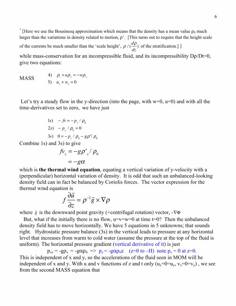
But, what if the initially there is no flow, u=v=w=0 at time t=0? Then the unbalanced density field has to move horizontally. We have 5 equations in 5 unknowns; that sounds right. Hydrostatic pressure balance (3s) in the vertical leads to pressure at any horizontal level that increases from warm to cold water (assume the pressure at the top of the fluid is uniform). The horizontal pressure gradient (vertical derivative of it) is just pxz = -gρx = -gαρ0. => px = -gαρ0z (z=0 to –H) note px = 0 at z=0. This is independent of x and y, so the accelerations of the fluid seen in MOM will be independent of x and y. With u and v functions of z and t only (ux=0=uy, vx=0=vy) , we see from the second MASS equation that

7

w = 0 for all time. This is ironic. Here we have a flow driven by its available potential energy (the ‘slumping’ of the fluid under gravity) and yet we find no vertical velocity. The reason is that the end-walls of this long channel of fluid have been left out of the problem. However far away they are, that is where the vertical velocity occurs (and its effects will eventually propagate into the region of interest). In this way we build a problem that we can solve, by using physical simplifications at the beginning. With w = 0 we have

which, after an x-differentiation, says that ρxt = -uρxx=0, so the horizontal density gradient does not change in time: the fluid moves simply, sliding horizontally in horizontal sheets. Now we combine to get a single equation in a single dependent variable: ∂(1)/∂z, using (3) is

utz − fvz = − pxz / ρ0

= gα

and use (2) to eliminate u, giving vztt + f 2vz = −gα f which is a nice forced oscillator equation for vz. To be clearer let us define a new variable for the vertical gradient of v, the vertical shear: ϕ = vz. Then ϕ tt + f 2ϕ = −gα f which is an equation independent of z as well as x and y. Forced O.D.E.’s often can be solved by finding an ‘homogeneous solution’ for the same lefthand side but zero for the righthand side, and then adding to it a ‘particular solution’ that takes care of the righthand side. In some problems these are also called ‘free-wave solution’ and ‘forced solution’. Very often the free-wave solution is necessary to satisfy some physical boundary conditions that the forced solution cannot cope with. In this spirit let ϕ = ϕH(t) + ϕP. We find ϕH = A sin ft + B cos ft, just some inertial oscillations, and the ‘forced’ or ‘particular’ or ‘steady’ part of the solution is ϕP = -gα/f which is the same thermal wind sheared velocity that we found earlier, could balance the intial, vertical isotherms (because ρx is the same).

8

Now we have initial conditions; for a second-order differential equation in time, two are required. With velocity vanishing at t=0, we have v=0 => ϕ(t=0) = 0 u=0 => ϕt(t=0) = 0 from the MOM equations. The first of these determines that B = gα/f while the second gives A = 0. The full solution is ϕ = (gα/f)(cos ft –1). From this we can determine all the other variables, by substituting in (1)-(4): v= (gαz/f)(cos ft –1) u = -(1/f)vt = +(gαz/f )sin ft ρ = ρ0 ((1 + αx + (gα2z/f2)(cos ft –1)) The fluid oscillates with the Coriolis frequency f, but not about zero: the dense fluid moves initially to the left and the constant-density surfaces flap back and forth about a mean position that is strongly inclined (downward/leftward). The mean velocity shear obeys the thermal-wind equation: fvz = −gα f and the full solution oscillates about this. Just as in a laboratory demonstration of the interleaving of water masses having different densities, the initially horizontal stratification builds a vertical stratification. To check signs, notice that the density at a point is always greater than/equal to the initial density because the cold fluid has slid to the left everywhere; thus the expression for ρ’ is always ≥0 (noting that z < 0). Similarly u ≤ 0 and v ≥ 0. Notice (lowest panel in the figure) that the same mean density field, with its sloping surfaces, could be in balance with an out-of the page geostrophic flow that was strong at the top of the fluid and decreased in speed with depth speed at greater depth: for example if one looks from the north at the Gulf Stream along the western boundary of the N Atlantic, the isotherms/isopycnals would appear similar to this figure but the velocity would be, as mentioned above, opposite to the deep current sketched below yet with the same vertical shear. The warm water would be that of the Sargasso Sea. The deeper velocity might actually be southward, for the cold water beneath is the flowing southward hugging the boundary, from the Labrador Sea.

9

So, how would you change the initial conditions for th theoretical model above to produce the out-of-the-page geostrophic flow, instead of into-the-page flow, from the same initial density field and zero velocity at t=0?

In the time mean, the buoyancy frequency resulting is N = (-g/ρ0 dρ0/dz)1/2

= gα/f. The mean slope of the isopycnal surfaces is ρX/ρZ = f2/gα = f/N. If we think of this mean slope as being H/L (H the fluid depth and L the x-displacement of the isopycnal at the bottom) we find NH/fL = 1 . This is a famous result which is found in many GFD problems. It is called Prandtl’s ratio or the Burger number, or the ratio of L to the baroclinic Rossby deformation radius, NH/f. There are several other interesting results here. The stability of stratified shear flows is governed, if rotation is ignored, by the Richardson number,

10

which, here, at any time, is equal to 1/2 . If the fluid is to be unstable in this sense to growing waves and turbulent overturning, Ri must fall below ¼ so it looks as if this flow is close to experiencing shear instability (the stratified version of Kelvin-Helmoltz instability. Just the mean thermal-wind flow has, itself, less shear and is more stable than the time-dependent ‘flapping venetian blind’ flow; Ri =1 for the mean flow. Geostrophic balance. Ignoring the oscillations (which we could remove by adding a little friction), this flow is a simple linear velocity gradient balancing a horizontal density gradient (which is at right angles to the vertically varying part of the velocity). The slumping of the fluid, with dense water underflowing less dense water, is arrested as the Coriolis force first turns the negative u velocity to the right, into a positive v-velocity. This v-velocity then feels a Coriolis force opposing the pressure gradient that produced it, and a balance is reached. Recall that gem-like relationship, eqn.(2), which says that if unopposed by a y-pressure gradient, as here, the v-velocity will be given by v = -fX, u = fY where X,Y = ∫(u,v) dt are the x- and y-displacements of a fluid particle. Unless the Coriolis force is balanced by a component of the pressure gradient, enormous velocities result from rather modest displacements (with f ≅ 10-4 sec-1, v = 10 m sec-1 for X =100 km lateral displacement); this is why flows have to be geostrophic if they are to go anywhere. There is not enough potential energy in the flow to provide the huge kinetic energy that would result from such unopposed displacements). The thermal wind, ‘geostrophy’ and hydrostatic balance are dominant force balances in the hydrographic section below. This solution and the analogous GFD lab experiment with a central source of buoyant water flowing radially outward, and forming a lens shaped vortex, gives us a reliable way of getting the signs right in thermal wind balance: in an observed flow, imaginel how the tilted density surfaces would move if the velocities were all set to zero: the surfaces would slump towards the horizontal (the Φ = constant geopotential surfaces), and the Coriolis force acting on those horizontal velocities show us the direction of the upper flow relative to the deep flow, for example northward in the warm (red) subtropical water on the eastern side of the N Atlantic at 600 N, relative to southward flows at depth. Thus from temperature/salinity/pressure observations we know the geostrophic velocity normal to a hydrographic section, to within an unknown function of the horizontal coordinate. This ‘reference velocity’ or ‘level of no motion’ is perhaps the most recurrent problem in physical oceanography over the past century. We now have ARGO velocities and NASA/European Space Agency satellite altimetry plus assimilation into

11

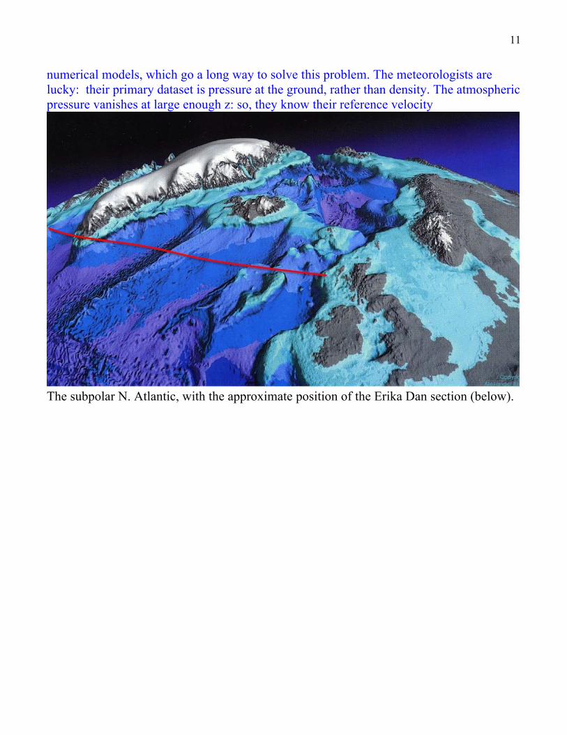
numerical models, which go a long way to solve this problem. The meteorologists are lucky: their primary dataset is pressure at the ground, rather than density. The atmospheric pressure vanishes at large enough z: so, they know their reference velocity

The subpolar N. Atlantic, with the approximate position of the Erika Dan section (below).

12

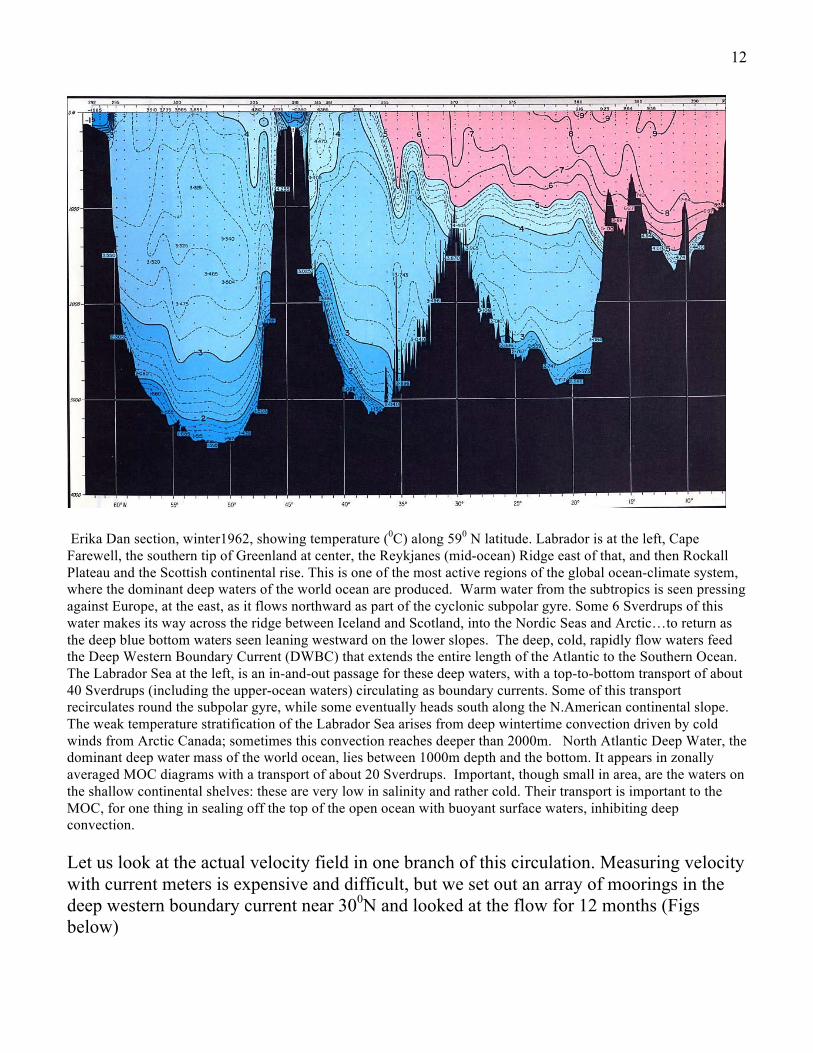
Erika Dan section, winter1962, showing temperature (0C) along 590 N latitude. Labrador is at the left, Cape Farewell, the southern tip of Greenland at center, the Reykjanes (mid-ocean) Ridge east of that, and then Rockall Plateau and the Scottish continental rise. This is one of the most active regions of the global ocean-climate system, where the dominant deep waters of the world ocean are produced. Warm water from the subtropics is seen pressing against Europe, at the east, as it flows northward as part of the cyclonic subpolar gyre. Some 6 Sverdrups of this water makes its way across the ridge between Iceland and Scotland, into the Nordic Seas and Arctic…to return as the deep blue bottom waters seen leaning westward on the lower slopes. The deep, cold, rapidly flow waters feed the Deep Western Boundary Current (DWBC) that extends the entire length of the Atlantic to the Southern Ocean. The Labrador Sea at the left, is an in-and-out passage for these deep waters, with a top-to-bottom transport of about 40 Sverdrups (including the upper-ocean waters) circulating as boundary currents. Some of this transport recirculates round the subpolar gyre, while some eventually heads south along the N.American continental slope. The weak temperature stratification of the Labrador Sea arises from deep wintertime convection driven by cold winds from Arctic Canada; sometimes this convection reaches deeper than 2000m. North Atlantic Deep Water, the dominant deep water mass of the world ocean, lies between 1000m depth and the bottom. It appears in zonally averaged MOC diagrams with a transport of about 20 Sverdrups. Important, though small in area, are the waters on the shallow continental shelves: these are very low in salinity and rather cold. Their transport is important to the MOC, for one thing in sealing off the top of the open ocean with buoyant surface waters, inhibiting deep convection. Let us look at the actual velocity field in one branch of this circulation. Measuring velocity with current meters is expensive and difficult, but we set out an array of moorings in the deep western boundary current near 300N and looked at the flow for 12 months (Figs below)

13

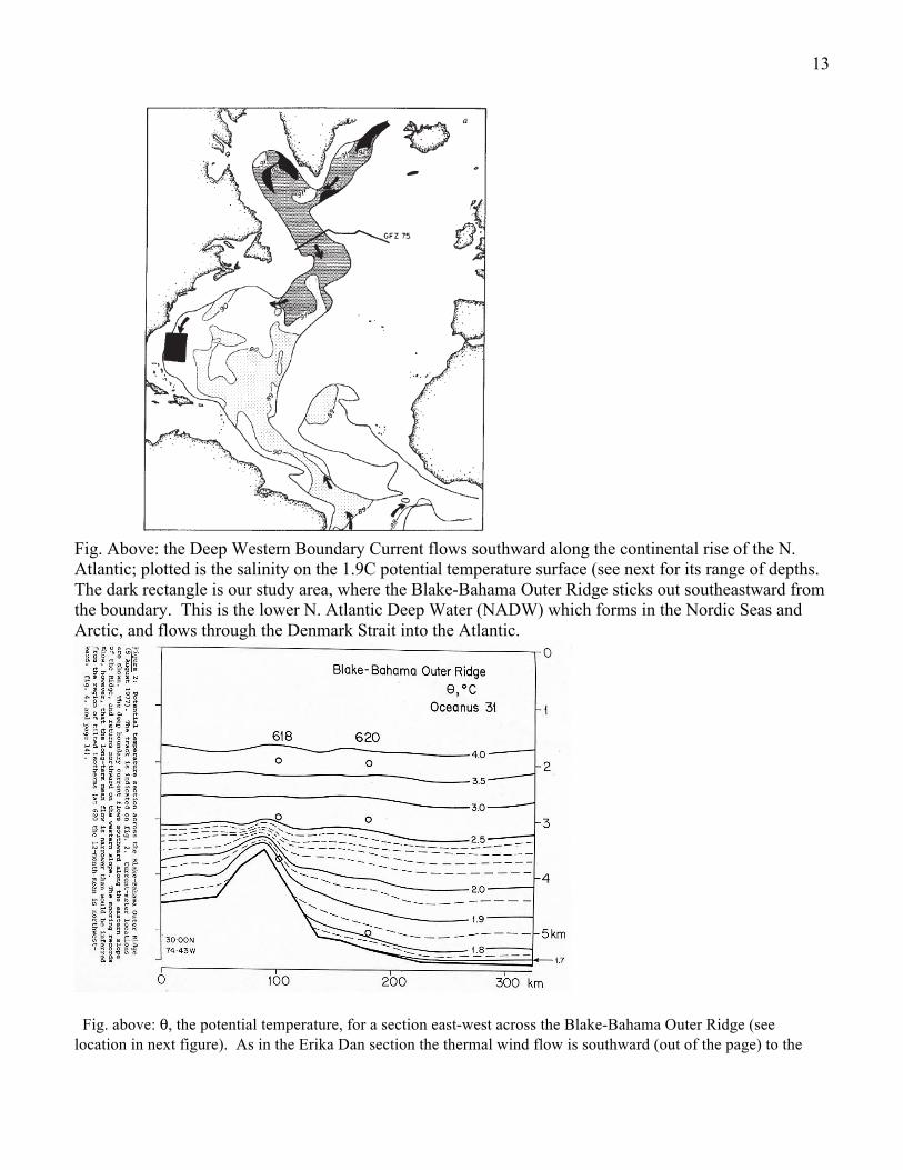
Fig. Above: the Deep Western Boundary Current flows southward along the continental rise of the N. Atlantic; plotted is the salinity on the 1.9C potential temperature surface (see next for its range of depths. The dark rectangle is our study area, where the Blake-Bahama Outer Ridge sticks out southeastward from the boundary. This is the lower N. Atlantic Deep Water (NADW) which forms in the Nordic Seas and Arctic, and flows through the Denmark Strait into the Atlantic.

Fig. above: θ, the potential temperature, for a section east-west across the Blake-Bahama Outer Ridge (see location in next figure). As in the Erika Dan section the thermal wind flow is southward (out of the page) to the

14

east of the ridge and northward its west. The Deep Western Boundary Current is winding around the tip of the Ridge on its way to the Equator here, as you see in the next figure. It might look as if this was a gravity-wave flow from left to right, but of course this is a much larger scale and the dominant geostropic flow is perpendicular to the sloping isotherms (really, isopycnals). The velocity increases downward toward the sea-floor, rather as in the theoretical model earlier in this lecture. If a barotropic (depth-independent) velocity were added to the flow, then this same density field could balance a northward current that increased in strength upward from the sea floor (on the east side of the Ridge). Notice that the horizontal velocity changes direction with depth as well as changing amplitude. This is ‘veering’ or ‘backing’ of the flow which is familiar in atmospheric science. It is an important consequence of thermal wind balance and tells us subtle things beyond just the horizontal velocity….can you imagine what how the sloping density surfaces would look, to cause veering or backing?

12-month mean currents (8/1977-7/1978) from four current meter moorings in the deep western boundary current. Depth of the instruments labeled in km. The deep jet follows the bottom topographic contours. The weaker flow at the upper levels veers in the sense of a stratified Taylor column. The 0.6 km-deep flow is consistent with an inflow joining the Gulf Stream to its west.

15

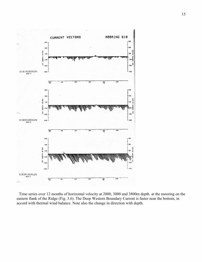
Time series over 12 months of horizontal velocity at 2000, 3000 and 3800m depth. at the mooring on the eastern flank of the Ridge (Fig. 3.6). The Deep Western Boundary Current is faster near the bottom, in accord with thermal wind balance. Note also the change in direction with depth.

16

Tritium tracer concentration in the section shown above. The maximum hugging the ridge shows the origins of this water at the ocean surface far to the north. This is Denmark Strait Overflow Water encountered at 59N in Fig. 3.5 (Jenkins and Rhines, Nature 1980). Tritium was injected into the atmosphere in the nuclear bomb tests of the 1950s/60s, and it entered the surface ocean both as rain and through water vapor, and run-off from ice-locked land surfaces. This demonstrated directly the ‘breathing’ of the ocean and the appearance of this signal some 3000 km to the south.