Getting Started with Expression Analysis in JMP …...GEttinG StArtEd with ExPrESSion AnAlySiS in...

WHITE PAPER

Getting Started with Expression Analysis in JMP® Genomics 4

i

GEttinG StArtEd with ExPrESSion AnAlySiS in JMP® GEnoMicS 4

Table of Contents

I. The JMP® Environment ............................................................................. 1a. File ..................................................................................................... 1b. Tables ................................................................................................. 2c. Rows .................................................................................................. 2d. Columns ............................................................................................. 2e. Analyze ............................................................................................... 3f. Graph .................................................................................................. 3g. Genomics Menu ................................................................................. 4

II. JMP® Genomics and SAS® ........................................................................ 5a. File Paths ........................................................................................... 5b. Configuration File and Temp Directory Setup..................................... 5

III. Importing Data ........................................................................................ 5a. Data Table Formats ............................................................................ 5b. Importing Affymetrix Data .................................................................. 6c. Importing Illumina Data ...................................................................... 8

IV. Data Analysis ........................................................................................ 10a. Basic Expression Workflow .............................................................. 10b. Results ............................................................................................. 15c. Quality Control Results ..................................................................... 16

i. Distribution ........................................................................................... 16

ii. PCA, Variance Estimates ..................................................................... 17

iii. Scatterplots ........................................................................................ 17

iv. Normalization ...................................................................................... 18

d. Results – ANOVA .............................................................................. 18i. Graphs ................................................................................................. 18

ii. Parsing Tables ..................................................................................... 19

iii. IPA Upload .......................................................................................... 22

e. Other Action Button Functions ......................................................... 22f. Pattern Discovery ............................................................................. 22

i. Hierarchical Clustering .......................................................................... 22

ii. K-Means Clustering ............................................................................. 24

V. Other Key Features in JMP® Genomics .................................................. 25a. Output Files ...................................................................................... 25b. Save/Load/Apply/Set as Default Buttons ......................................... 25

VI. Summary ............................................................................................... 26


This white paper is intended to give existing and new customers and evaluators a brief overview of the JMP Genomics solution and an introduction to some of the new features in JMP Genomics 4.0. For more detailed information about specific processes, please consult the JMP Genomics User Guide, found under Genomics > Documentation and Help.

I. The JMP® Environment

a. File

The File menu contains options for saving and opening data sets. When saving data sets in JMP Genomics, the standard File > Save As… option can be used. In the “Save as type” box, choose SAS Data Set. Clear the “Preserve SAS variable names” box.

Figure 1

The File > Save as SAS Data Set function will use SAS® routines to save data and

can sometimes be useful, particularly with large data files.

As part of the configuration following installation of JMP Genomics, the JMP preferences should have been set to those that are optimal for JMP Genomics. If you have not done so, or have changed the preferences, click File > Set Genomics Preferences now. If you wish to change the default locations for files, configure a proxy server for Internet access, or control the archiving of SAS code generated in JMP Genomics, this can be done using File > Configure Genomics Settings.

1

2


b. Tables

The Tables menu contains numerous functions for manipulating JMP tables. Keep in mind that when a SAS data set is open in JMP, JMP treats it as a JMP table, and so these functions are active. We will show the Subset function later in this document, and other functions such as Tables > Join or Tables > Concatenate can also be useful. Note that many of these functions appear to be redundant with those in Genomics > Data Set Utilities. Choosing the Data Set Utilities functions is recommended when tables are too large to open in memory, or when it is important to maintain SAS variable (column) names in a proper format.

c. Rows

The Rows menu contains a number of functions for manipulating row states in JMP tables. Clicking Rows > Data Filter allows simple and dynamic selection of rows in a data table for subsequent subset creation and is very useful in filtering graphical output in JMP Genomics. Note that the Rows menu appears only when a table is open in the workspace.

d. Columns

Similar to Rows, the Cols menu contains functions for manipulating columns in an open data table. The Cols > Reorder Columns function can be especially useful when a group of columns to be deleted all start with the same prefix. Note that individual columns can also be deleted by selecting the column in the left pane, right-clicking, then choosing Delete Columns.

Another important tool is Cols > Recode. Often categorical data can have various values depending on how it was entered. For example, a Gender column may contain values M, Male, F and Female. JMP will treat all of these as different levels of Gender. The Recode function makes it simple to create consistency without having to edit many rows of a table manually.

Figure 2

Note also in the left pane of an open data table that columns have symbols that signify different data types. These indicate if the data in the columns is Numeric, with its associated subtypes, or Character (categorical data). There is a difference between SAS and JMP in that JMP does recognize subtypes of numeric data, whereas SAS only differentiates between Character and Numeric data.


3

Occasionally in JMP Genomics, data will be misclassified during the import process. For example, there may be a variable with values of 0, 1 and 2 that needs to be treated as numeric for SAS processes, but as part of data collection, missing data was represented with an “N.A.” This variable will then be classified as categorical. To change this, double-click the variable header and change the data type to the desired format.

Figure 3

e. Analyze

A number of analysis options are available in the Analyze menu. The Distribution function is used extensively in output graphs in JMP Genomics and can be very helpful in assessing design files and other data for consistency of values. Click Analyze > Distribution, fill in the “Y, Columns” box with the desired variables and click “OK” to generate the output.

Figure 4

f. Graph

JMP Genomics processes have integrated graphical output, but the tools available under the Graph menu are useful for generating alternative visualizations of JMP Genomics output. In particular, Graph > Graph Builder is a tool that provides a flexible and intuitive interface to generate many different types of plots. To explore

4


the Graph Builder, bring any data table into focus by clicking it, and then launch the Graph Builder. Drag columns from the selection box into different parts of the graph area to generate different types of plots. You may right-click on points to change graph type.

Figure 5

Two other tools that can be useful for genomics data reside in the Graph menu: Graph > Overlay Plot is good for generating scatterplots and positional plots along chromosomes, and Graph > Cell Plot can be used to generate heat maps.

g. Genomics Menu

The Genomics menu contains the majority of the functions specific to JMP Genomics. Note that most of these processes use JMP dialogs to gather parameters, call SAS code behind the scenes and launch results in JMP. The functions relevant to expression analysis are discussed below.t


5

II. JMP® Genomics and SAS®

a. File Paths

By default, JMP Genomics is installed in the path C:\Program Files\SAS\JMP\8\Genomics, unless a different path is chosen during installation. Under the Genomics directory are a number of folders, including the ProcessLibrary, which contains programs that specify the structure of the interfaces and underlying SAS programs, and the MacroLibrary, which contains other general macros used by JMP Genomics processes. You may view these macros. Scripts specifying process dialogs are found under the user area of Documents and Settings, in the directory C:\Documents and Settings\<username>\Local Settings\Application Data\JMPG\ProcessLibrary.

b. Configuration File and Temp Directory Setup

The SAS temp directory is the work directory which holds temporary files created during an analysis. You may look in this folder while an analysis is running to see the files being built by selecting Genomics > Documentation and Help > Open SAS Temporary Folder. If any processes are terminated with Windows Task Manager before completion, the temporary files will not be deleted and should be deleted manually by accessing the temp directory. For more information on the configuration file settings, please refer to the installation and configuration guides for SAS.

III. Importing Data

a. Data Table Formats

For expression and exon analysis, JMP Genomics requires two files: a design file and a data file. The design file contains all the information regarding the sample attributes. You should include as much information as possible about your experiment, including technical variables (e.g., date or batch), as well as experimental and clinical variables. Including this type of information will make it easier to understand the sources of variance in the experiment when you run quality control processes. The design file has two required columns or variables. The Array column is numeric and has a unique number for each array. The ColumnName column contains a unique identifier for each array. JMP Genomics software contains tools to create these variables, found in the Experimental Design submenu.

The tall data files used for expression analysis contain the gene or probeset intensities in rows and data from individual samples in columns. The ColumnName variable is used to merge design information with data during analysis, so each

6


column name in the data table must match a ColumnName value in the design file exactly. Note that the data file can contain more samples than are in the design file, allowing you to restrict analyses to a particular subset simply by subsetting the design file. Conversely, the design file cannot contain more ColumnName rows than there are samples in the data file.

b. Importing Affymetrix Data

In preparation for importing Affymetrix expression data, the Affymetrix Experimental Design Wizard can help create a design file from Affymetrix Array Attribute (ARR) files from Affymetrix’s Expression Console or from existing text or Excel file formats. Note that when importing design information from text or Excel files, your design file template must contain a column labeled File or FileName, containing the file names of all the arrays in the study, and at least one column with design information that will be used in statistical tests (e.g., Treatment). In this example, we will import from ARR files. These are from the MPRO data sets available at Affymetrix.com. Select Genomics > Experimental Design File > Affymetrix Experimental Design File Wizard. Click “Next” and in the following window, name your study and choose either “Extract information from ARR Files (AGCC format)” or “Import design information from an existing text, CSV, or Excel file.” We will select the ARR file option.

Figure 6

In the next window, indicate that the data comes from an Expression array rather than a SNP or Exon array, and click “Next.” The following window is titled “Step 2,” and it asks you to indicate the directory containing your data and ARR files. Note that if both CEL and CHP types are present in that directory, you will be asked to select which files to use. If multiple CHP types are present, you will need to select which ones to include in your design. After this step, an open design file will be displayed. At any time before you click “Save,” you may add columns or make modifications to


7

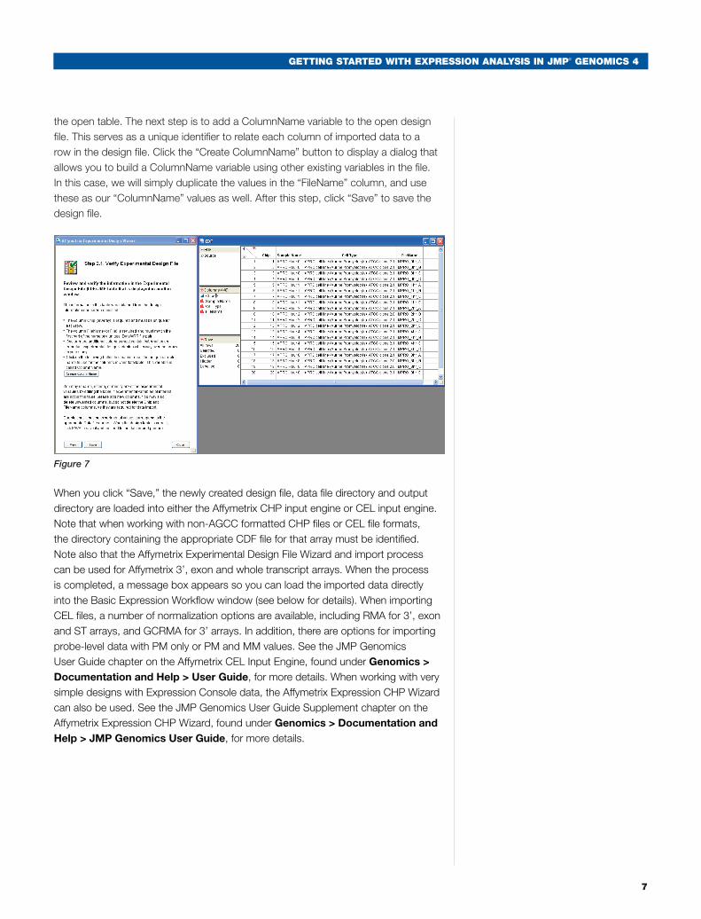
the open table. The next step is to add a ColumnName variable to the open design file. This serves as a unique identifier to relate each column of imported data to a row in the design file. Click the “Create ColumnName” button to display a dialog that allows you to build a ColumnName variable using other existing variables in the file. In this case, we will simply duplicate the values in the “FileName” column, and use these as our “ColumnName” values as well. After this step, click “Save” to save the design file.

Figure 7

When you click “Save,” the newly created design file, data file directory and output directory are loaded into either the Affymetrix CHP input engine or CEL input engine. Note that when working with non-AGCC formatted CHP files or CEL file formats, the directory containing the appropriate CDF file for that array must be identified. Note also that the Affymetrix Experimental Design File Wizard and import process can be used for Affymetrix 3’, exon and whole transcript arrays. When the process is completed, a message box appears so you can load the imported data directly into the Basic Expression Workflow window (see below for details). When importing CEL files, a number of normalization options are available, including RMA for 3’, exon and ST arrays, and GCRMA for 3’ arrays. In addition, there are options for importing probe-level data with PM only or PM and MM values. See the JMP Genomics User Guide chapter on the Affymetrix CEL Input Engine, found under Genomics > Documentation and Help > User Guide, for more details. When working with very simple designs with Expression Console data, the Affymetrix Expression CHP Wizard can also be used. See the JMP Genomics User Guide Supplement chapter on the Affymetrix Expression CHP Wizard, found under Genomics > Documentation and Help > JMP Genomics User Guide, for more details.

8


c. Importing Illumina Data

You can import Illumina data by simply using the output files from BeadStudio or GenomeStudio software. JMP Genomics can accept either the Final Report format from the export wizard or standard TXT file formats. To import Illumina expression data, go to Genomics > Import > Illumina > Expression. Select the appropriate file for the “Sample Gene Import File.” Set “Files of Type” to “Text Import Files (*.TXT, *.CSV, *.DAT).”

Figure 8

The file in the “Samples File” box should be exported from BeadStudio or GenomeStudio software. If no samples file is available, a design file template containing only ColumnName and Array will be created. This template can then be completed manually using the tools in the Experimental Design File menu. The Options tab allows for filtering based on detection p-values and optional log2

transformation of data. Note that any negative values remaining after filtering will be set to missing after log2 conversion.

Figure 9


9

tinStarted with Expression Analysis in JMP® Genomics

On the Output tab you can determine settings for naming files and formatting annotation data in the imported Illumina data set. Keep in mind that selecting the option “Include in output data set” will include annotation and data in the main data table for only those probes which passed the filtering criteria you set. However, choosing the option to create a separate annotation data set will allow you to retain annotation information for all the probes.

Figure 10

10


IV. Data Analysis

a. Basic Expression Workflow

Following import of Illumina or Affymetrix data as described above, a pop-up window appears that you can use to automatically load the Basic Expression Workflow. Note that after Affymetrix file import you can choose between the Basic Expression and Basic Exon Workflow, depending on the type of data set you imported. For Illumina data, only the Basic Expression Workflow is available.

Click “Basic Expression Workflow.” The dialog is automatically populated with the experimental design file, the data file and the output directory where your input data set is stored. You may elect to change the output directory at this time if you wish to store your results in a different location.

Figure 11

Fill in the “Study Name” and “Label Variable” boxes.

In the Experimental Design tab, select the variables by which to color QC plots and grouped sets of scatterplots.


11

Figure 12

The Quality Control and Normalization tab is where you can select post-import normalization, if desired, and choose when to run QC processes: before or after normalization, or both.

G

Figure 13

The ANOVA tab is where you set up your model and desired comparisons.

12


Figure 14

The “Class Variables” box should contain variables whose different levels you want to compare, plus any other variable which may have some impact on your expression levels. Note that Class Variables are always categorical. For example, a treatment variable may include values of Control, Treatment 1, Treatment 2, etc., but not continuous values of 0, 0.15 or 0.30. In this case, we have only one class variable, “Sample_Name.” In the “Model these Fixed Effects” box, you should specify variables that may have an impact on expression values. This must include at least one Class Variable specified as a Fixed Effect. Other Fixed Effects can be included, as can continuous variables. If you want to specify interaction or nested variables, the syntax is A*B or A(B), respectively. JMP Genomics will automatically call the proper process depending on the complexity of your model.

“Adjust Variability for these Random Effects” is where you specify a variable that affects your expression analysis and contributes unwanted variance. For example, arrays that are run in batches over a period of time may have some differences due to the batch effect. Batch can be listed as a Class Variable, and the variance due to the batch effect will be removed when it is listed as a Random Effect in the model.

The “Separate and Journal Results by Chromosome” option is useful for large arrays, allowing the results to be interrogated separately for each chromosome. In order to choose this option, you must specify a chromosome variable either in the input data set on the General tab or in the annotation file on the Annotation tab.

The LSMeans tab contains options for forming pairwise comparisons and volcano plots.


13

Figure 15

In the “Estimate LSMeans for these Fixed Effects” box, type the names of any variables or interactions for which a comparison is desired. If you are forming differences with a control, specify the control value, as JMP Genomics will choose one by default if one is not entered. Note that the value must be in double quotes and must match exactly the design table value.

The Multiple Testing tab contains options for controlling the multiple testing correction that is applied to the collection of results. If you requested volcano plots on the LS Means tab, then the correction is applied to all pairwise comparisons. Otherwise, the correction is applied to the fixed effects and covariates specified in the ANOVA tab.

Figure 16

14


On the Annotation tab, you can specify an annotation data set with supplemental information such as gene symbols, accession numbers and other identifying information. Information from this file will be appended to output tables to facilitate interpretation of results. This annotation data set can come from array manufacturers, GEO or other sources. If GenBank accession numbers, gene symbols or LocusLink IDs are present in the annotation file, then specifying them properly in the dialog on the Annotation tab will allow the creation of buttons in the output that link from specific results in plots to the appropriate Web databases.

Figure 17

If you decide not to merge annotation while running the workflow, you may merge annotation information after analysis.

The Tracks tab enables the creation of graphical displays of transcript information to embellish positional plots. For further information, see the JMP Genomics User Guide.


15

b. Results

Basic Expression Workflow results are returned in journal format.

Figure 18

Click “Open Workflow Dialog” to launch the Workflow Builder.

Figure 19

The “Workflow to Run” box contains the processes used in the Basic Expression Workflow. A process can be opened by highlighting the process name, then clicking “Edit.” The settings within each process can be modified, saved and the analysis

16


rerun. Note that if you repeat an analysis but do not assign a different name for the output files (found in the Options tab), the initial results will be overwritten. To rerun the workflow, we recommend that you specify a new Workflow Folder location and select “Change Output Folder to Workflow Folder in Settings Moved to Right Panel.”

c. Quality Control Results

i. Distribution

Click “Results” under “DataDistribution” to open the distribution plots. Two graphs are created: a side-by-side box plot and an overlay of the arrays’ kernel density estimates. Drill down on the box plots by clicking the red triangle to get more information, such as quantiles. The resulting values can be converted into a JMP table by right-clicking and selecting “Make into Data Table.”

Figure 20

The other graph, “Overlayed Kernel Density Estimates,” is a view of the intensity profiles of the arrays in the data set.

Figure 21


17

In the available action buttons resulting from this process, the “Filter Intensities” process can be opened directly from these results. With this application, you can modify or remove low or high values, and delete genes which do not meet certain criteria.

Additionally, any of the arrays that are deemed to be outliers can be removed from future analyses. Select the arrays to be excluded by clicking them in the Kernel Density Estimates plot, then click “Create Subset Experimental Design Data Set, Excluding Selected Rows.” The resulting truncated design data set can be used with the original tall data file in new analyses to exclude the outlying arrays.

When you are finished viewing the results of the distribution analysis, return to the workflow results journal and click “Close All Other Windows” to clear the JMP environment.

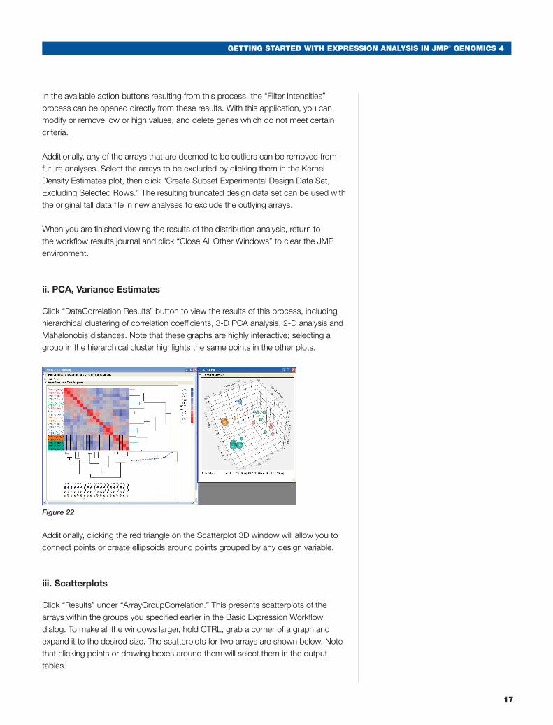
ii. PCA, Variance Estimates

Click “DataCorrelation Results” button to view the results of this process, including hierarchical clustering of correlation coefficients, 3-D PCA analysis, 2-D analysis and Mahalonobis distances. Note that these graphs are highly interactive; selecting a group in the hierarchical cluster highlights the same points in the other plots.

Figure 22

Additionally, clicking the red triangle on the Scatterplot 3D window will allow you to connect points or create ellipsoids around points grouped by any design variable.

iii. Scatterplots

Click “Results” under “ArrayGroupCorrelation.” This presents scatterplots of the arrays within the groups you specified earlier in the Basic Expression Workflow dialog. To make all the windows larger, hold CTRL, grab a corner of a graph and expand it to the desired size. The scatterplots for two arrays are shown below. Note that clicking points or drawing boxes around them will select them in the output tables.

18


Figure 23

iv. Normalization

The workflow has a number of standardization options for normalization. You can perform QC before and after normalization, if desired. If you would like to perform a normalization process that is not in the workflow, additional options can be found in Genomics > Normalization. Following normalization, the resulting output file can be rerun in the workflow, with or without an additional normalization step.

d. Results – ANOVA

i. Graphs

A number of graphs are created following ANOVA analysis. First, volcano plots for all comparisons are shown.

Figure 24

The x-axis displays differences (log2 ratios); that is, a difference of 1 is approximately the same as a twofold change. The y-axis shows the –log10 (p-value) for the comparison between the two groups. The dashed red line is the value for significance


19

with the correction for false discovery rate. Note that the p-values are not adjusted for false discovery rate, only the threshold for significance. To adjust the p-values themselves, use the “P-Value Adjustment” AP, found under Genomics > Row-by-Row Modeling.

Highlight points with your mouse to highlight corresponding rows in the table. You can create a new data table containing only these points using the Tables > Subset function.

The hierarchical clustering diagram contains the results of any probesets with at least one significant difference between analysis groups. Highlighting a branch of this graph also highlights the corresponding probesets in the output table. A subset of highlighted probesets can be created as described above.

The parallel plots of standardized and unstandardized Least Squares Means also contain only the significant probesets. With a large number of significant probesets, these plots can be difficult to interpret. Small numbers of probesets can be graphed following parsing of tables, or the Data Filter can be used to pare down the plots by selecting samples with differences or p-values in certain ranges for the comparisons of interest.

The distributions of r-square and residuals can be helpful in understanding the quality of the results. In general, distributions skewed to a high r-square and low residual indicate that most of the variance was contained within your model. The opposite finding indicates that there may be sources of variances in your data that are not accounted for in your model.

ii. Parsing Tables

You can easily parse results tables using JMP Genomics tools. In the ANOVA results table, each probeset is given a significance index of 0 or 1 for each comparison, with 1 indicating significance. We can use these significance indicators and other variables such as differences to obtain subset tables. First, click in a results table with the suffix _owa or _ars to make sure it is the active table. Go to Genomics > Annotation Analysis > Venn Diagram. Select up to five significance indices from the list of columns. For two- and three-way diagrams, selecting “Proportional Areas” causes the regions of the diagram to be drawn with areas proportional to the number of results they contain. Click “Edit” at the bottom of the plot to control colors, labels and label placement.

20


Figure 25

The Venn Diagram is interactive with the results table. In this case, a group of 74 probesets is highlighted. Clicking Tables > Subset will create a data table containing only these probesets. Next, go to Tables > Tabulate. Highlight all the significance indices and move them to the “Drop Zone for Rows.” Select “Add Columns by Categories.” The values of 0 and 1 for each comparison are shown. These are also interactive, and can be used to select multiple groups as an “Or” query.

Figure 26

Next, select Rows > Data Filter. Using this tool, we will select those probesets from the Hour 2 vs. Hour 0 comparison whose differences are greater than 1 or less than -1. First, highlight the appropriate significance index and difference value. Use the CTRL key to make this multiple selection. Click “Add.” Next, click “+” and select the same two variables again. While holding SHIFT, click “Add.” This will add the comparison as an “Or” statement. Now, highlight the “1” for the significance index, and click over the less than or greater than values and replace them with 1 or -1 as appropriate.


21

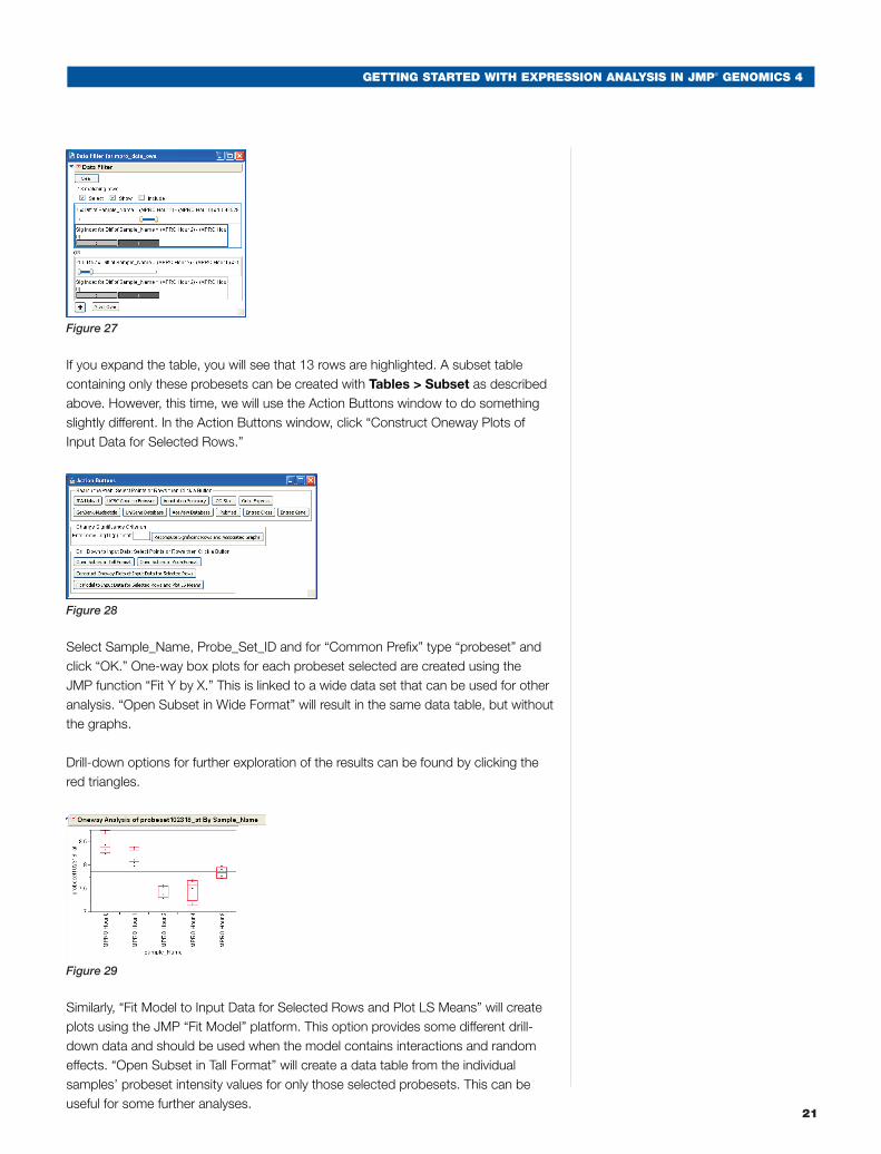
Figure 27

If you expand the table, you will see that 13 rows are highlighted. A subset table containing only these probesets can be created with Tables > Subset as described above. However, this time, we will use the Action Buttons window to do something slightly different. In the Action Buttons window, click “Construct Oneway Plots of Input Data for Selected Rows.”

Figure 28

Select Sample_Name, Probe_Set_ID and for “Common Prefix” type “probeset” and click “OK.” One-way box plots for each probeset selected are created using the JMP function “Fit Y by X.” This is linked to a wide data set that can be used for other analysis. “Open Subset in Wide Format” will result in the same data table, but without the graphs.

Drill-down options for further exploration of the results can be found by clicking the red triangles.

Figure 29

Similarly, “Fit Model to Input Data for Selected Rows and Plot LS Means” will create plots using the JMP “Fit Model” platform. This option provides some different drill-down data and should be used when the model contains interactions and random effects. “Open Subset in Tall Format” will create a data table from the individual samples’ probeset intensity values for only those selected probesets. This can be useful for some further analyses.

22


iii. IPA Upload

The results of the significant genes table, or a subset of that table, can be easily used to upload data to Ingenuity Pathway Analysis. Select Genomics > Annotation Analysis > IPA Upload. Choose the significant genes data table. This will have the suffix _sig in the title. If you want to upload all the data, select Rows > Row Selection > Select All Rows from the menu. You can also parse the table in preparation for upload using a method previously described. Select “IPA Upload” from the Action Buttons menu. The table with the selected probesets will automatically load. The Affymetrix Probe_Set_ID is the Gene/Protein identifier, and we will upload the differences as log ratios. On the Options tab, select the appropriate array version.

Figure 30

Clicking “Upload to IPA” will result in IPA opening and the data loading into the initial upload page. Note that you do need an IPA license to work with the data inside the IPA application. You may request a trial license from Ingenuity at https://analysis.ingenuity.com/pa/account/signup.html.ing Started with Expression Analysis in

JMP® Genomics

e. Other Action Button Functions

The Annotation Summary in the Action Button menu will create a dynamic Web page with links to selected Web sites. The other buttons will open a Web page for each selected row, so use these only when selecting a limited number of probesets.

f. Pattern Discovery

i. Hierarchical Clustering

Hierarchical clustering can be performed on tall or wide data sets, depending on the desired results. In this instance, we will cluster a data set with probesets that were significant in the Hour 2 vs. Hour 0, with a difference greater than 0.5 or less than -0.5. This data set was generated using the “Create Wide Data Set” Action Button.


23

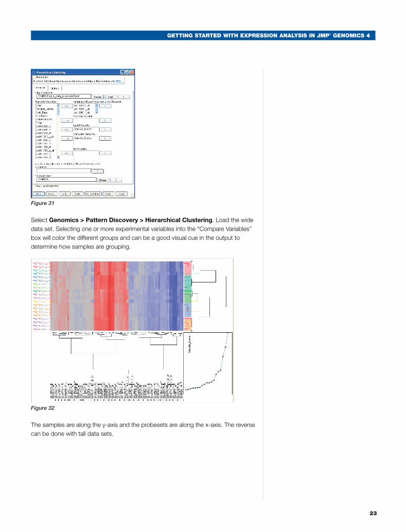
Figure 31

Select Genomics > Pattern Discovery > Hierarchical Clustering. Load the wide data set. Selecting one or more experimental variables into the “Compare Variables” box will color the different groups and can be a good visual cue in the output to determine how samples are grouping.

Figure 32

The samples are along the y-axis and the probesets are along the x-axis. The reverse can be done with tall data sets.

24


ii. K-Means Clustering

K-means clustering will group probesets according to their patterns. The user can choose how many clusters to create, or the number of clusters can be determined on the basis of the correlation between probesets. Select Genomics > Pattern Discovery > K-Means Clustering. Select the significant results table for clustering. Either the mean values or the standardized mean values can be used.

Figure 33

On the Analysis tab, select “Automated Radius K Means.” The correlation radius is a measure of how closely you would like the probesets within a cluster to correlate. Higher correlations will give fewer probesets per cluster and more clusters, and lower correlations will have more probesets per cluster and fewer clusters. Select “Center Rows” if working with mean values, and clear this option if you are working with standardized mean values.

Figure 34

The counts for each cluster, and the clusters themselves, are presented as part of the results. The probesets within each cluster can be easily parsed using Rows > Data Filter and selecting the “Cluster” variable on the output table.


25

V. Other Key Features in JMP® Genomics

a. Output Files

The results from an analysis in JMP Genomics do not have to be recreated each time you wish to view analysis results. Every time a process is run, a JSL file is created. This JSL file is linked to output tables. Running this JSL file in JMP Genomics will recreate the analysis results.

Figure 35

In the example above, running the JSL by double-clicking it in Windows Explorer or opening it within JMP Genomics will recall the results from the Principal Components Analysis. Additionally, log files and SAS settings files are automatically created for each analysis. You can also optionally archive a copy of the SAS code run from each process by selecting this option under File > Set Genomics Preferences. These steps can assist you in retracing the steps in your analysis workflows.

b. Save/Load/Apply/Set as Default Buttons

At the bottom of each application window, in addition to the “Run” button, are the “Save,” “Load,” “Apply” and “Set as Default” buttons.

Figure 36

The “Save ...” button allows you to save the settings (i.e., dialog choices), either complete or partial, that are currently in this process window. The “Load ...” button allows you to load saved settings. Many users find it useful to create a separate “Settings” directory in the directory used for analysis results. By creating settings that are similar in name to the output files, you can retain a record of analysis workflows. The “Apply” button allows you to broadcast choices made in the current process dialog to different processes. After clicking the “Apply” button, new processes opened in that session will autofill with the input file(s), output path and any other values in common with the applied values. This can be very useful when working though a data set without the workflow application. If new choices are made, clicking “Apply” again will update to the new settings. Selecting Genomics > Clear Parameter Defaults will clear all temporary settings. The “Set as Default” button saves the current dialog choices as default values that will autofill whenever you open the same process. The “Reset” button clears the current dialog choices and reloads the default values.

26


VI. Summary

This paper introduces the Basic Expression workflow, hierarchical clustering and K-means clustering. After getting familiar with the Basic Expression workflow, advanced users may wish to investigate the Expression QC workflow and the Expression Statistics workflow, which offer greater flexibility and more options.

Further and more detailed information can be found in the JMP Genomics User Guide. There are sample data files for one-color and two-color expression analyses that are installed with the software, and saved settings that may be loaded to run sample analyses for these data sets. To access the sample settings, click “Load …” at the bottom of any JMP Genomics dialog, and then click “Example Settings” to navigate to the right folder.

SAS and all other SAS Institute Inc. product or service names are registered trademarks or trademarks of SAS Institute Inc. in the USA and other countries. ® indicates USA registration.

Other brand and product names are trademarks of their respective companies. Copyright © 2009, SAS Institute Inc. All rights reserved. 104083_543904_0709

SAS Institute Inc. World Headquarters +1 919 677 8000 To contact your local JMP office, please visit www.jmp.com

Getting Started with Expression Analysis in JMP …...GEttinG StArtEd with ExPrESSion AnAlySiS in...

Documents

Transcript of Getting Started with Expression Analysis in JMP …...GEttinG StArtEd with ExPrESSion AnAlySiS in...