Getting Out Of A Tight Spot: Physics Of Flow Through ...
178
Getting Out Of A Tight Spot: Physics Of Flow Through Porous Materials A dissertation presented by Sujit Sankar Datta to The Department of Physics in partial fulfillment of the requirements for the degree of Doctor of Philosophy in the subject of Physics Harvard University Cambridge, Massachusetts September 2013
Transcript of Getting Out Of A Tight Spot: Physics Of Flow Through ...

Getting Out Of A Tight Spot:Physics Of Flow Through Porous Materials
A dissertation presented
by
Sujit Sankar Datta
to
The Department of Physics
in partial fulfillment of the requirements
for the degree of
Doctor of Philosophy
in the subject of
Physics
Harvard University
Cambridge, Massachusetts
September 2013

c©2013 - Sujit Sankar Datta
All rights reserved.

Dissertation Advisor: David A. Weitz Sujit Sankar Datta
Getting Out Of A Tight Spot:
Physics Of Flow Through Porous Materials
AbstractWe study the physics of flow through porous materials in two different ways: by di-
rectly visualizing flow through a model three-dimensional (3D) porous medium, and by
investigating the deformability of fluid-filled microcapsules having porous shells.
In the first part of this thesis, we develop an experimental approach to directly visu-
alize fluid flow through a 3D porous medium. We use this to investigate drainage, the
displacement of a wetting fluid from a porous medium by a non-wetting fluid, as well as
secondary imbibition, the subsequent displacement of the non-wetting fluid by the wet-
ting fluid. We characterize the intricate morphologies of the non-wetting fluid ganglia left
trapped within the pore space, and show how the ganglia configurations vary with the wet-
ting fluid flow rate. We then visualize the spatial fluctuations in the fluid flow, both for
single- and multi-phase flow. We use our measurements to quantify the strong variability
in the flow velocities, as well as the pore-scale correlations in the flow. Finally, we use our
experimental approach to study the simultaneous flow of botha wetting and a non-wetting
fluid through a porous medium, and elucidate the flow instabilities that arise for sufficiently
large flow rates.
In the second part of this thesis, we study the mechanical properties of porous spherical
microcapsules. We first introduce emulsions, and describe how their rheology depends on
the microscopic interactions between the drops comprisingthem. We then study the for-
mation and buckling of one class of microcapsule – nanoparticle-coated emulsion drops.
iii

Abstract
We also use double emulsions, drops within drops, as templates to form another class of
microcapsule – drops coated with thin, porous, polymer shells. We investigate how, under
sufficient osmotic pressure, these microcapsules buckle, and show how the inhomogeneity
in the shell structure can guide the folding pathway taken bya microcapsule as it buckles.
Finally, we study the expansion and rupture of microcapsules under the influence of elec-
trostatic forces. For both buckling and expansion, we show that the deformation dynamics
can be understood by coupling shell theory with Darcy’s law for flow through the porous
microcapsule shell.
iv

Contents
Title Page . . . . . . . . . . . . . . . . . . . . . . . . . . . . . . . . . . . . . . iAbstract . . . . . . . . . . . . . . . . . . . . . . . . . . . . . . . . . . . . . . .iiiTable of Contents . . . . . . . . . . . . . . . . . . . . . . . . . . . . . . . . . .vCitations to Previously Published Work . . . . . . . . . . . . . . . . .. . . . . viiAcknowledgments . . . . . . . . . . . . . . . . . . . . . . . . . . . . . . . . . .xDedication . . . . . . . . . . . . . . . . . . . . . . . . . . . . . . . . . . . . . .xii
1 Introduction 11.1 Visualizing flow through a model 3D porous medium . . . . . . .. . . . . 11.2 Deformations of porous microcapsules . . . . . . . . . . . . . . .. . . . . 3
2 Experimental approach to visualizing multi-phase flow in athree-dimensionalporous medium 52.1 Preparation of the medium . . . . . . . . . . . . . . . . . . . . . . . . . .62.2 Formulating refractive index-matched fluids . . . . . . . . .. . . . . . . . 62.3 3D visualization using confocal microscopy . . . . . . . . . .. . . . . . . 82.4 Measurement of permeability . . . . . . . . . . . . . . . . . . . . . . .. . 9
3 Drainage in a three-dimensional porous medium 103.1 Drainage in a homogeneous porous medium . . . . . . . . . . . . . .. . . 123.2 Drainage in a stratified porous medium . . . . . . . . . . . . . . . .. . . . 16
4 Imbibition in a three-dimensional porous medium 264.1 Pore-scale dynamics of secondary imbibition . . . . . . . . .. . . . . . . 284.2 Trapped oil ganglia configurations . . . . . . . . . . . . . . . . . .. . . . 324.3 Physics of ganglion mobilization . . . . . . . . . . . . . . . . . . .. . . . 38
5 Spatial fluctuations of fluid velocities in flow through a three-dimensional porousmedium 455.1 Visualizing single-phase flow . . . . . . . . . . . . . . . . . . . . . .. . . 465.2 Quantifying correlations in the flow . . . . . . . . . . . . . . . . .. . . . 515.3 Visualizing multi-phase flow . . . . . . . . . . . . . . . . . . . . . . .. . 55
v

Contents
6 Fluid breakup during simultaneous two-phase flow through athree-dimensionalporous medium 586.1 Visualizing multi-phase flow . . . . . . . . . . . . . . . . . . . . . . .. . 606.2 Understanding the fluid breakup . . . . . . . . . . . . . . . . . . . . .. . 646.3 State diagram for the connected-to-broken up transition . . . . . . . . . . . 67
7 Rheology of emulsions 717.1 Formulation of emulsions . . . . . . . . . . . . . . . . . . . . . . . . . .. 737.2 Frequency-dependent mechanical response . . . . . . . . . . .. . . . . . 757.3 Strain-dependent mechanical response . . . . . . . . . . . . . .. . . . . . 777.4 Time scales of the structural relaxation . . . . . . . . . . . . .. . . . . . . 84
8 Buckling and crumpling of nanoparticle-coated droplets 898.1 Formulation of Pickering emulsions . . . . . . . . . . . . . . . . .. . . . 918.2 Volume-controlled morphological transitions . . . . . . .. . . . . . . . . 928.3 Size-dependent morphologies . . . . . . . . . . . . . . . . . . . . . .. . . 98
9 Buckling of inhomogeneous microcapsules 1059.1 Microcapsule fabrication . . . . . . . . . . . . . . . . . . . . . . . . .. . 1079.2 Onset of microcapsule buckling . . . . . . . . . . . . . . . . . . . . .. . 1139.3 Dynamics of microcapsule buckling . . . . . . . . . . . . . . . . . .. . . 1169.4 Shell inhomogeneities guide microcapsule deformations . . . . . . . . . .122
10 Expansion and rupture of pH-responsive microcapsules 12610.1 Microcapsules composed solely of a pH-responsive polymer . . . . . . . .12810.2 Hybrid microcapsules . . . . . . . . . . . . . . . . . . . . . . . . . . . .. 133
Bibliography 141
vi
Citations to Previously Published Work
Most of Chapters 2-10 are based on the following papers:
Chapters 2, 3, and 4:“Visualizing multi-phase flow and trapped fluid configurationsin a model three-dimensional porous medium”,A. T. Krummel∗, S. S. Datta∗, S. Munster, and D. A. Weitz,AIChE Journal59, 1022 (2013) *Equal contribution.
Chapter 3:“Drainage in a model stratified porous medium”,S. S. Dattaand D. A. Weitz,EPL101, 14002 (2013).
Chapters 3 and 4:“Mobilization of a trapped non-wetting fluidfrom a three-dimensional porous medium”,S. S. Datta, T. S. Ramakrishnan, and D. A. Weitz, to be submitted (2013).
Chapter 5:“Spatial fluctuations of fluid velocities in flowthrough a three-dimensional porous medium”,S. S. Datta, T. S. Ramakrishnan, and D. A. Weitz,Physical Review Letters111, 064501 (2013).
Chapter 6:“Fluid breakup during simultaneous two-phase flowthrough a three-dimensional porous medium”,S. S. Datta, J. B. Dupin, and D. A. Weitz, to be submitted (2013).
Chapter 7:“Rheology of attractive emulsions”,S. S. Datta, D. D. Gerrard, T. S. Rhodes, T. G. Mason, and D. A. Weitz,Physical Review E, 84, 041404 (2011).
vii
Citations to Previously Published Work
Chapter 8:“Controlled buckling and crumpling of nanoparticle-coated droplets”,S. S. Datta, H. C. Shum, and D. A. Weitz,Langmuir, 26, 18612 (2010).
Chapter 9:“Controlling release from double emulsion-templated microcapsules”,S. S. Datta∗, A. Abbaspourrad∗, E. Amstad, J. Fan, S-H Kim, M. Romanowsky,H. C. Shum, B. J. Sun, A. S. Utada, M. Windbergs, S. Zhu, and D. A. Weitz,to be submitted (2013) *Equal contribution.
Chapter 9:“Delayed buckling and guided folding of inhomogeneous capsules”,S. S. Datta∗, S-H Kim∗, J. Paulose∗,A. Abbaspourrad, D. R. Nelson, and D. A. Weitz,Physical Review Letters109, 134302 (2012) *Equal contribution.
Chapter 10:“Expansion and rupture of pH-responsive microcapsules”,S. S. Datta∗, A. Abbaspourrad∗, and D. A. Weitz,submitted,Materials Horizons(2013) *Equal contribution.
Chapter 10:“Controlling release from pH-responsive microcapsules”,A. Abbaspourrad∗, S. S. Datta∗, and D. A. Weitz,submitted,Langmuir(2013) *Equal contribution.
Citations to other work co-authored during the course of thedegree, not included in thisthesis:
“Thermally switched release from nanoparticle colloidosomes”,S. Zhu∗, J. Fan∗, S. S. Datta, X. Guo, M. Guo, and D. A. Weitz,in press,Advanced Functional Materials(2013) *Equal contribution.
“Ultrathin shell double emulsion-templated giant unilamellar lipid vesicleswith controlled microdomain formation”,L. R. Arriaga,S. S. Datta, S. H. Kim, E. Amstad,T. E. Kodger, F. Monroy, and D. A. Weitz, submitted,Small(2013).
viii

Citations to Previously Published Work
“Microfluidic fabrication of stable gas-filled microcapsulesfor acoustic contrast enhancement”,A. Abbaspourrad∗, W. J. Duncanson∗, N. Lebedeva, S. H. Kim, A. Zhushma,S. S. Datta, S. S. Sheiko, M. Rubinstein, and D. A. Weitz,in press,Langmuir(2013) *Equal contribution.
“Controlling the morphology of polyureamicrocapsules using microfluidics”,I. Polenz,S. S. Datta, and D. A. Weitz, to be submitted (2013).
“The microfluidic arrayed-post device: high throughputproduction of viscous single drops”,E. Amstad,S. S. Datta, and D. A. Weitz, to be submitted (2013).
“Wetting and energetics in nanoparticle etching of graphene”S. S. Datta, Journal of Applied Physics108, 024307 (2010).
ix

Acknowledgments
I am lucky to have had the opportunity to interact with so manyamazing people during
the course of my Ph.D.
First and foremost, Dave. Thank you for introducing me to thesemicolon. More im-
portantly, thank you for teaching me how to think. I will always have your voice in my
head, pushing me to be the best scientist and person I can be. Your energy and creativity
will always be an inspiration as I constantly ask myself: what would Dave do?
Dave always says that if he’s the only professor you interactwith at Harvard, you’re
wasting your time. I’ve learned so much from a number of otherprofessors: David Nel-
son, Jim Rice, Howard Stone, L. Mahadevan, Michael Brenner,Zhigang Suo, and John
Hutchinson. Thank you all for taking the time to educate me and for putting up with my
constant questions. I am especially grateful to ProfessorsNelson and Rice for taking the
time to be on my thesis committee and provide enormous amounts of support.
The Weitz lab is a fantastic place to do science, and I would like to thank all the Weit-
zlabbers with whom I’ve interacted over the years. I am particularly grateful to Ali Ab-
baspourrad, Esther Amstad, Tommy Angelini, Laura Arriaga,Oni Basu, Harry Chiang,
Wynter Duncanson, Jean-Baptiste Dupin, Dustin Gerrard, Erin Hannen, Shin-Hyun Kim,
Dorota Koziej, Amber Krummel, Tina Lin, Peter Lu, Anderson Shum, Joris Sprakel, Jim
and Connie (and Claire!) Wilking, Huidang Zhang, and undoubtedly many other equally
deserving people whose names just aren’t coming to my sleep-deprived mind right now,
for exciting collaborations, interesting discussions, orjust making life in the lab so much
more fun. I would also like to thank Laura for taking the time to go through and comment
on this thesis. And Peter, for always keeping things interesting, and for inspiring the title
of this thesis.
x

Acknowledgments
I’ve had a ton of fun discussing science with a number of people outside of the Weitzlab,
as well: Jayson Paulose, Tom Mason, and Alberto Fernandez-Nieves. I have also benefited
tremendously from fantastic collaborations and discussions with the researchers down the
street at Schlumberger-Doll Research: T. S. Ramakrishnan,Jeff Paulsen, Dave Johnson,
Yi-Qiao Song, and Martin Hurlimann.
Finally, I’d like to thank all of my friends for enriching my life. I would particularly
like to thank the crew at Redline Fight Sports, who maintained my sanity and taught me
how to be resilient by letting me beat them up (or beating me up) on a regular basis. And
of course, my family, for always loving and supporting me.
xi

Somewhere, something incredible is waiting to be known.
–Carl Sagan
xii

Chapter 1
Introduction
1.1 Visualizing flow through a model 3D porous medium
Filtering water, squeezing a wet sponge, and brewing coffeeare all familiar examples
of forcing a fluid through a porous medium. This process is also crucial to many tech-
nological applications, including geological flows, the operation of packed bed reactors,
chromatography, fuel cells, chemical release from colloidal capsules, and even nutrient
transport through mammalian tissues [1, 2, 3, 4, 5, 6, 7]. Such flows, when sufficiently
slow, are typically modeled using Darcy’s law,∆p = µqL/k, whereµ is the fluid dynamic
viscosity andk is the absolute permeability of the porous medium; this law relates the pres-
sure drop∆p across a lengthL of the entire medium to the flow velocityq, averaged over a
sufficiently large length scale. However, while appealing,this simple continuum approach
does not explicitly treat local pore-scale variations in the flow, which may arise as the fluid
navigates the tortuous 3D pore space of the medium. Such flow variations can have signifi-
cant practical consequences; for example, they may result in spatially heterogeneous solute
1

Chapter 1: Introduction
transport through a porous medium. This impacts diverse situations ranging from the dry-
ing of building materials [8], to biological flows [6, 9, 7], to geological tracer monitoring
[1]. Moreover, many situations, such as groundwater aquifer remediation, geological CO2
sequestration, oil recovery, and the operation of trickle bed reactors, involve the flows of
multiple immiscible fluids [1]. This imparts further complexity to the flow. For example,
the multi-phase flow can lead to the formation, trapping, or mobilization of discrete gan-
glia of a non-wetting fluid within the porous medium [10, 11, 12, 13, 14, 15, 16, 17, 18].
This phenomenon is particularly relevant to oil recovery, where over 90% of the oil within
a reservoir can remain trapped after primary recovery. Understanding the physics of flow
through a 3D porous medium, on scales ranging from that of an individual pore to the scale
of the entire medium, is therefore both intriguing and important.
Some of this complex flow behavior can be visualized in two-dimensional (2D) mi-
cromodels [14, 19]; however, a complete understanding of the physics underlying the for-
mation and trapping of ganglia requires experimental measurements on 3D porous media
[16, 20, 13, 21]. Optical techniques typically cannot be used to directly image the flow
through such media due to the light scattering caused by the differences in the indices of
refraction between the different fluid phases and the solid material making up the medium
itself. Instead, magnetic resonance imaging (MRI) [22, 23] and X-ray micro computer to-
mography (X-rayµCT) [24, 25, 26, 27] have been used to visualize either the bulk flow
dynamics, or some pore-scale behavior, within 3D porous media; however, fast visual-
ization, both at pore-scale resolution and over the scale ofthe entire medium, is typically
challenging. While theoretical models and numerical simulations provide crucial additional
insight [28, 29, 30, 31, 32, 33, 34, 35, 36, 37, 1, 38, 39, 40], fully describing the disordered
2

Chapter 1: Introduction
structure of the medium can be challenging. Consequently, despite its enormous practical
importance, a complete understanding of flow within a 3D porous medium remains elusive.
In the first part of this thesis, we report an approach to visualize single- and multi-phase
flow through a model 3D porous medium, at scales ranging from that of individual pores
to that of the entire medium. We first describe the experimental approach [Chapter 2].
We use this approach to investigate drainage, the displacement of a wetting fluid from a
porous medium by a non-wetting fluid [Chapter 3], as well as secondary imbibition, the
subsequent displacement of the non-wetting fluid by the wetting fluid [Chapter 4]. We
characterize the intricate morphologies of the non-wetting fluid ganglia left trapped within
the pore space, and show how the ganglia configurations vary with the wetting fluid flow
rate. We then visualize the spatial fluctuations in the fluid flow, both for single- and multi-
phase flow [Chapter 5]. We use our measurements to quantify the strong variability in
the flow velocities, as well as the pore-scale correlations in the flow. Finally, we use our
experimental approach to study the simultaneous flow of botha wetting and a non-wetting
fluid through a porous medium [Chapter 6], and elucidate the flow instabilities that arise
for sufficiently large flow rates.
1.2 Deformations of porous microcapsules
A microcapsule is a micrometer-scale liquid drop surrounded by a solid shell; because
this shell acts as a barrier separating the core from the external environment, microcap-
sules are promising candidates for encapsulating and controllably releasing many impor-
tant active materials. These include surfactants for enhanced oil recovery [41], agricul-
tural chemicals [42, 43, 44, 45, 46, 47], food additives [48, 49, 50, 51], pharmaceuticals
3
Chapter 1: Introduction
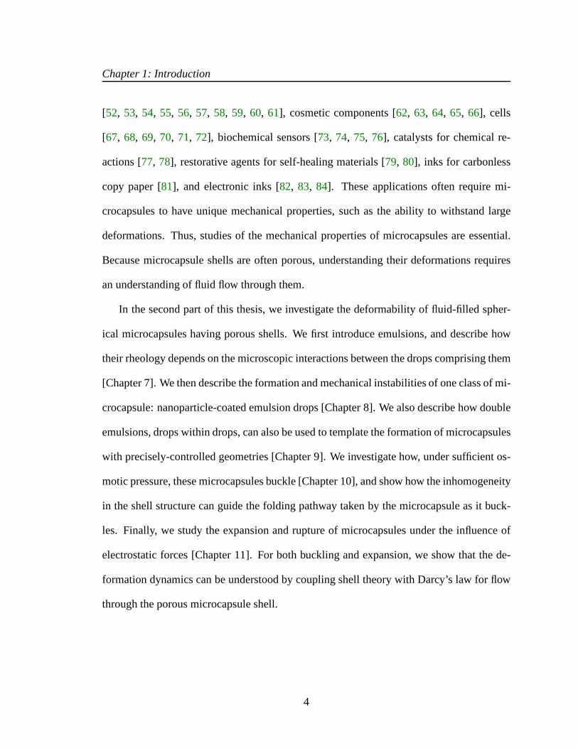
[52, 53, 54, 55, 56, 57, 58, 59, 60, 61], cosmetic components [62, 63, 64, 65, 66], cells
[67, 68, 69, 70, 71, 72], biochemical sensors [73, 74, 75, 76], catalysts for chemical re-
actions [77, 78], restorative agents for self-healing materials [79, 80], inks for carbonless
copy paper [81], and electronic inks [82, 83, 84]. These applications often require mi-
crocapsules to have unique mechanical properties, such as the ability to withstand large
deformations. Thus, studies of the mechanical properties of microcapsules are essential.
Because microcapsule shells are often porous, understanding their deformations requires
an understanding of fluid flow through them.
In the second part of this thesis, we investigate the deformability of fluid-filled spher-
ical microcapsules having porous shells. We first introduceemulsions, and describe how
their rheology depends on the microscopic interactions between the drops comprising them
[Chapter 7]. We then describe the formation and mechanical instabilities of one class of mi-
crocapsule: nanoparticle-coated emulsion drops [Chapter8]. We also describe how double
emulsions, drops within drops, can also be used to template the formation of microcapsules
with precisely-controlled geometries [Chapter 9]. We investigate how, under sufficient os-
motic pressure, these microcapsules buckle [Chapter 10], and show how the inhomogeneity
in the shell structure can guide the folding pathway taken bythe microcapsule as it buck-
les. Finally, we study the expansion and rupture of microcapsules under the influence of
electrostatic forces [Chapter 11]. For both buckling and expansion, we show that the de-
formation dynamics can be understood by coupling shell theory with Darcy’s law for flow
through the porous microcapsule shell.
4

Chapter 2
Experimental approach to visualizing
multi-phase flow in a three-dimensional
porous medium
In this Chapter1, we describe the experimental approach by which we visualize single-
and multi-phase flow through a model 3D water-wet porous medium. We match the refrac-
tive indices of the wetting fluid, the non-wetting oil, and the porous medium; this enables
us to directly image the structure of the medium, and the multi-phase flow within it, in 3D
using confocal microscopy.
1Based on “Visualizing multi-phase flow and trapped fluid configurations in a model three-dimensionalporous medium”, A. T. Krummel∗, S. S. Datta∗, S. Munster, and D. A. Weitz,AIChE Journal59, 1022(2013) *Equal contribution.
5
Chapter 2: Experimental approach to visualizing multi-phase flow in a three-dimensionalporous medium
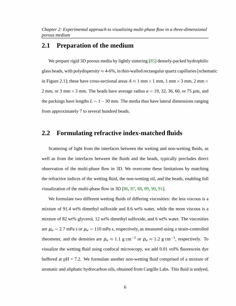
2.1 Preparation of the medium
We prepare rigid 3D porous media by lightly sintering [85] densely-packed hydrophilic
glass beads, with polydispersity≈ 4-6%, in thin-walled rectangular quartz capillaries [schematic
in Figure 2.1]; these have cross-sectional areasA≈ 1 mm×1 mm, 1 mm×3 mm, 2 mm×
2 mm, or 3 mm×3 mm. The beads have average radiusa = 19, 32, 36, 60, or 75µm, and
the packings have lengthsL ∼ 1−30 mm. The media thus have lateral dimensions ranging
from approximately 7 to several hundred beads.
2.2 Formulating refractive index-matched fluids
Scattering of light from the interfaces between the wettingand non-wetting fluids, as
well as from the interfaces between the fluids and the beads, typically precludes direct
observation of the multi-phase flow in 3D. We overcome these limitations by matching
the refractive indices of the wetting fluid, the non-wettingoil, and the beads, enabling full
visualization of the multi-phase flow in 3D [86, 87, 88, 89, 90, 91].
We formulate two different wetting fluids of differing viscosities: the less viscous is a
mixture of 91.4 wt% dimethyl sulfoxide and 8.6 wt% water, while the more viscous is a
mixture of 82 wt% glycerol, 12 wt% dimethyl sulfoxide, and 6 wt% water. The viscosities
areµw = 2.7 mPa s orµw = 110 mPa s, respectively, as measured using a strain-controlled
rheometer, and the densities areρw ≈ 1.1 g cm−3 or ρw ≈ 1.2 g cm−3, respectively. To
visualize the wetting fluid using confocal microscopy, we add 0.01 vol% fluorescein dye
buffered at pH = 7.2. We formulate another non-wetting fluid comprised of a mixture of
aromatic and aliphatic hydrocarbon oils, obtained from Cargille Labs. This fluid is undyed,
6

Chapter 2: Experimental approach to visualizing multi-phase flow in a three-dimensionalporous medium
Figure 2.1:Overview of the experimental approach. (Left) Schematic illustrating thestructure of a typical 3D porous medium and imaging of flow within it using confocalmicroscopy. (Top Right) Three optical slices, of thickness2.0 µm and lateral area 912µm × 912 µm, taken at three different depths within a medium comprisedof beads withaverage radiusa = 75 µm. The medium has been saturated with dyed wetting fluid; theblack circles show the beads, while the bright space in between shows the imaged porevolume. (Bottom Right) 3D reconstruction of a porous mediumcomprised of beads withaverage radiusa = 75 µm, with cross-sectional area 910µm × 910µm; the image showsthe reconstruction of a section 350µm high for clarity.
has a viscosityµnw = 16.8 mPa s, and a densityρnw ≈ 0.8 g cm−3. The interfacial tension
between the wetting and non-wetting fluids isγ ≈ 13.0 mN m−1, as measured using a du
Nouy ring; this value is similar to the interfacial tensionbetween crude oil and water [92].
We use confocal microscopy to estimate the three-phase contact angle made between the
wetting fluid and a clean glass slide in the presence of the non-wetting fluid,θ ≈ 5◦.
7

Chapter 2: Experimental approach to visualizing multi-phase flow in a three-dimensionalporous medium
2.3 3D visualization using confocal microscopy
We exploit the close match between the refractive indices ofthe fluorescently-dyed
wetting fluid and the glass beads to visualize the structure of the porous medium in 3D.
Prior to each experiment, the porous medium is evacuated under vacuum and saturated with
CO2 gas; this gas is soluble in the wetting fluid, preventing the formation of any trapped gas
bubbles. We then fill the medium with the fluorescently-dyed wetting fluid by imbibition;
a similar approach is used to saturate a rock core prior to core-flood experiments. We use a
confocal microscope to image an optical slice, either 2µm, 7µm, or 11µm thick, spanning
a lateral area of 912µm×912µm within the medium, and identify the glass beads by their
contrast with the dyed wetting fluid, as exemplified by the slices shown in Figure 2.1. To
visualize the pore structure in 3D, we acquire a 3D image stack of multiple slices, each
spaced by several micrometers along thez direction, within the porous medium, as shown
in 2.1. We use these slices to reconstruct the 3D structure ofthe medium [Figure 2.1]. The
packing of the beads is disordered; to quantify the porosity, φ , of this packing, we integrate
the fluorescence intensity over all slices making up a stack.To visualize the pore structure
of the entire medium, we acquire additional stacks, at the samez positions, but at multiple
xy locations spanning the entire width and length of the medium. We findφ = 41±3%
independent of position along the length of the medium, as shown in Figure 2.2; this is
comparable to the porosity of highly porous sandstone [93]. Moreover,φ is similar for
different realizations of a porous medium, as shown by the different symbols in Figure 2;
this illustrates the reproducibility of our protocol.
We repeatedly acquire these image stacks during the multi-phase flow. The non-wetting
oil is undyed; we thus visualize its flow using its additionalcontrast in the measured pore
8

Chapter 2: Experimental approach to visualizing multi-phase flow in a three-dimensionalporous medium
Figure 2.2:Porosity φ of porous media is the same for different positions and realiza-tions. We findφ = 41±3% at multiple positions along the length of the porous media, andfor different porous media prepared in the same way (different symbols).
volume. Moreover, in some cases, we take movies of multiple optical slices, acquired at
the samexyzposition, with∼ 10 ms time resolution.
2.4 Measurement of permeability
To quantify the bulk transport behavior, we use differential pressure sensors to measure
the pressure drop∆P across a porous medium. We saturate the medium with the wetting
fluid and vary the volumetric flow rateQw over the range∼ 0.2−50 mL h−1; by measur-
ing the proportionate variation in∆P, we determine the single-phase permeability of the
medium,k≡ µw(QwL/A)/∆P; for example, for a medium composed ofa = 19 µm radius
beads in a capillary with cross-sectional areaA = 9 mm2, we measurek = 1.67 µm2. The
permeability of a disordered packing of monodisperse spheres is typically estimated us-
ing the Kozeny-Carman relation,k = 145
φ3a2
(1−φ)2 [94]; this yieldsk = 1.59 µm2, in excellent
agreement with our measured value.
9

Chapter 3
Drainage in a three-dimensional porous
medium
One important class of multi-phase flow is drainage, the displacement of a wetting fluid
from a porous medium by an immiscible non-wetting fluid. To displace the wetting fluid
from a pore, the pressure in the non-wetting fluid at the pore entrance must exceed the
pressure in the wetting fluid, as schematized in Figure 3.1; this pressure difference is given
by Pγ ∼ γ/at , whereγ is the interfacial tension between the fluids andat is the radius of the
pore entrance [95, 96, 97]. For a homogeneous porous medium, characterized by pores of
a single average size,Pγ is typically much larger than the viscous pressure associated with
flow into a pore,∼ µnw(Qnw/φA)/at, whereµnw is the viscosity of the non-wetting fluid,
Qnw is the imposed volumetric flow rate of the non-wetting fluid,A is the medium cross-
sectional area, andφ is the medium porosity. Consequently, the flow path taken during
drainage depends primarily on the slight pore-scale variations ofat [98, 99, 100, 101, 102].
However, many porous media are stratified, consisting of parallel strata characterized by
10

Chapter 3: Drainage in a three-dimensional porous medium
Figure 3.1: Schematic showing invasion of a pore by the non-wetting fluid, shown in or-ange. The pore is initially filled with the wetting fluid, shown in blue. If the non-wettingfluid pressure is too small, the fluid interface is not sufficiently curved, and the non-wettingfluid does not invade the pore (left). If the non-wetting fluidexceeds a threshold, the curva-ture of the fluid interface is sufficient for the non-wetting fluid to invade the pore, displacingthe wetting fluid in the process (right).
different average pore sizes [1, 103, 104]. Such additional variation in the pore structure,
on scales much larger than a single pore, may strongly modifythe flow behavior [105,
106, 107, 108, 109, 110, 111, 101]. Despite its enormous practical importance, a clear
picture of how the subtle interplay between capillary and viscous forces determines the flow
through a 3D stratified porous medium remains elusive. This requires direct visualization
of the multi-phase flow, both at the scale of the individual pores and the overall strata.
Unfortunately, the medium opacity typically precludes such visualization. As a result,
knowledge of how exactly drainage proceeds within a stratified porous medium is missing.
In this Chapter2, we use confocal microscopy to investigate drainage withina 3D porous
medium. We first study drainage within a homogeneous porous medium. We then study
drainage within a heterogeneous porous medium having parallel strata oriented along the
flow direction. For the heterogeneous case, we find that for sufficiently small capillary
2Based on “Drainage in a model stratified porous medium”,S. S. Dattaand D. A. Weitz,EPL 101,14002 (2013), “Mobilization of a trapped non-wetting fluid from a three-dimensional porous medium”,S. S.Datta, T. S. Ramakrishnan, and D. A. Weitz, to be submitted (2013),and “Visualizing multi-phase flow andtrapped fluid configurations in a model three-dimensional porous medium”, A. T. Krummel∗, S. S. Datta∗,S. Munster, and D. A. Weitz,AIChE Journal59, 1022 (2013) *Equal contribution.
11

Chapter 3: Drainage in a three-dimensional porous medium
numbers,Ca, the non-wetting fluid flows only through the coarsest stratum of the medium.
By contrast, above a thresholdCa, the non-wetting fluid is also forced laterally into part
of the adjacent, finer strata. By balancing the viscous pressure driving the flow with the
capillary pressure required to invade a pore, we show how both the thresholdCa and the
spatial extent of the invasion depend on the pore sizes, cross-sectional areas, lengths, and
relative positions of the strata. Our results thus help elucidate how the path taken by the
non-wetting fluid is altered by stratification in a 3D porous medium.
3.1 Drainage in a homogeneous porous medium
To mimic the migration of a non-wetting fluid into a homogeneous geological forma-
tion, we first drain a homogeneous 3D porous medium [schematized in Figure 3.2(a)],
initially saturated with the dyed low-viscosity wetting fluid, with the undyed non-wetting
oil at a volumetric flow rateQnw = 1 mL h−1. To quantify the competition between the
viscous and capillary forces at the pore scale, we calculatethe corresponding capillary
number,Ca≡ µnw(Qnw/A)/γ ∼ 4.0×10⁻⁵. This definition ofCa frequently occurs in the
literature, and we therefore use it in this and the next Chapter to facilitate comparison be-
tween our results and previous work. However, we note that a more accurate representation
of the viscous force would also incorporate the medium porosity φ : the ratio of the viscous
and capillary pressures then scales asµnw(Qnw/φA)/atγ/at
= µnw(Qnw/φA)/γ instead. We use
this more accurate definition ofCa in Chapter 6.
ForCa∼ 4.0×10⁻⁵, the oil displaces the wetting fluid through a series of intermittent,
abrupt bursts into the pores; this indicates that a threshold capillary pressure difference must
build up in the oil before it can invade a pore [112]. This pressure is given by 2γ cosθ/at ,
12

Chapter 3: Drainage in a three-dimensional porous medium
Figure 3.2:Visualizing drainage within a 3D porous medium(a) Schematic of experi-mental setup. We directly visualize the flow within the medium using confocal microscopy.The pore space is initially saturated with the fluorescently-dyed wetting fluid, which is dis-placed by the undyed non-wetting oil. (b) Optical section through part of the medium,taken as the oil displaces the wetting fluid atQnw = 1 mL h−1. Section is obtained at afixed z position, away from the lateral boundaries of the medium. Bright areas show thepore space, saturated with the fluorescently-dyed wetting fluid, and the black circles showcross-sections of the beads making up the medium. Additional black areas show the in-vading oil. The path taken by the oil varies spatially, as seen in the region spanned by thearrow. (c) Optical section through the same part of the medium, taken after invasion by≈ 9 pore volumes of the oil. Some wetting fluid remains trapped in the crevices and poresof the medium, as indicated. (d) Time sequence of zoomed confocal micrographs, withthe pore space subtracted; binary images thus show oil in black as it bursts into the pores.Time stamp indicates time elapsed after subtracted frame. Upper and lower arrows in thelast frame show wetting fluid trapped in a crevice or in a pore,respectively. Scale bars in(b-c) and (d) are 500µm and 200µm, respectively. Imposed flow direction in all imagesis from left to right.
13

Chapter 3: Drainage in a three-dimensional porous medium
Figure 3.3: Pore-scale dynamics of drainage depend strongly onCa. Images showmultiple frames, taken at different times, of a single optical slice. The slice is 11µm thickand is imaged within a porous medium comprised of beads with average radiusa= 75µm,with cross-sectional width 3 mm and height 1 mm. The first frame in each sequence showsthe imaged pore space, saturated with dyed wetting fluid; thedark circles are the beads,while the additional dark areas show the invading undyed oil. The beads, and the saturatedpore space in between them, are subtracted from the subsequent frames in each sequence;thus, the dark areas in the subsequent frames only show the invading oil. Direction of bulkoil flow is from left to right. The final frame shows the unchanging steady state. Labelsshow time elapsed after first frame. (a) At lowCa= 6×10⁻⁵, the oil menisci displace thewetting fluid through a series of abrupt bursts into the pores, and the invading fluid interfaceis ramified over the scale of multiple pores. (b) At highCa= 4×10⁻³, the oil bursts occursimultaneously, and the invading fluid interface is more compact over the scale of multiplepores. In both cases, we observe a∼ 1 µm-thick layer of the wetting fluid coating the beadsurfaces after oil invasion, indicated in the last frame of each sequence. Scale bars are 200µm.
14

Chapter 3: Drainage in a three-dimensional porous medium
whereat ≈ 0.16a is the typical radius of a pore entrance,a is the average bead radius, and
θ is the three-phase contact angle [14, 97, 96, 113, 114]. The bursts are typically only one
pore wide [115], but can span many pores in length along the direction of thelocal flow
[third frame of Figure 3.3(a)]; moreover, the oil remains continually connected during flow.
Because the packing of the beads is disordered,at varies from pore to pore, forcing the path
taken by the invading oil to similarly vary spatially, as exemplified by the optical sections in
Figures 3.2(b, d) and 3.3 [98, 100, 99, 101, 102]. Consequently, the interface between the
oil and the displaced wetting fluid interface is ramified [tipof the arrow in Figure 3.2(b)].
As the oil continues to drain the medium, it eventually fills most of the pore space, as
shown in Figure 3.2(c); however, the smallest pores remain filled with the wetting fluid
[rightmost indicator in Figure 3.2(c) and lower arrow in Figure 3.2(d)]. Thin layers of
the wetting fluid,≈ 1 µm thick, remain trapped in the crevices of the medium, surround-
ing the oil in the pores [shown by the leftmost indicator in Figure 3.2(c), the upper arrow
in Figure 3.2(d), and the indicator in Figure 3.3(a)]; because we use optical imaging, we
can resolve this layer to within hundreds of nanometers. This observation provides di-
rect confirmation of the predictions of a number of theoretical calculations and numerical
simulations [14, 116, 117, 118, 17, 119, 120, 121, 122, 123, 124, 125, 18, 126].
As the oil bursts into a pore at a speedv, it displaces the wetting fluid, initially con-
tained within the pore, over a lengthl through the porous medium. This length can be
estimated by balancing the threshold capillary pressure, approximately 2γ/at , with the
viscous pressure required to displace the wetting fluid overthe lengthl , approximately
µwφvl/k, whereµw is the viscosity of the wetting fluid andk is the medium permeability;
this yieldsl ≈ (2γk)/µwφvat . Our experimental approach enables us to directly visual-
15

Chapter 3: Drainage in a three-dimensional porous medium
ize, and quantify the speed of, individual bursts. For a porous medium witha = 75 µm,
k = 75 µm2, φ = 0.41, and cross-sectional widthw= 3 mm, we measure a maximum burst
speedv≈ 10 mm s−1; this corresponds to wetting fluid flow overl ≈ (2γk)/µwφvat ∼ 10
mm. While the details of this flow are complex, this simple scaling estimate suggests that
the wetting fluid is displaced over a length scale comparableto the width of the porous
medium, spanning many pores in size; this observation is consistent with previous mea-
surements of pressure fluctuations during drainage [127], as well as imaging of drainage
through a monolayer of glass beads [128].
To explore the dependence of the water displacement on flow conditions, we visualize
the drainage for varyingCa. Unlike the lowCa case, the oil bursts are not successive
during drainage at higher values ofCa∼ 10−4−10−2; instead, neighboring bursts occur
simultaneously, typically in the bulk flow direction [Figure 3.3(b)]. As a result, over the
scale of multiple pores, the interface between the invadingoil and the wetting fluid is more
compact; this behavior reflects the increasing contribution of the viscous pressure in the
invading oil at higherCa [98, 129, 128]. As in the lowCacase, we do not observe evidence
for oil pinch off or subsequent reconnection; interestingly, this behavior is in contrast to the
prediction that the oil can be pinched off during drainage [130, 131, 132]. Similar to the
low Cacase, we observe a∼ 1 µm thick layer of the wetting fluid coating the bead surfaces
after oil invasion [18, 15, 133, 17], as indicated in the rightmost panels of Figure 3.3.
3.2 Drainage in a stratified porous medium
To create stratified porous media, we arrange the beads into parallel strata characterized
by different bead sizes and the same lengthL; the interface between the strata runs along
16

Chapter 3: Drainage in a three-dimensional porous medium
Figure 3.4:Geometry of a stratified 3D porous medium.(Left) Schematic of a stratifiedporous medium, with parallel strata comprised of differently-sized beads. (Right) Opticalsection acquired within a porous medium with a coarse and a fine stratum; the pore spaceis saturated with the fluorescently-dyed wetting fluid, and the black circles show crosssections of the beads making up the medium.
the direction of fluid flow. The effect of stratification on theflow behavior is exemplified
by flowing the non-wetting oil through a wetting-fluid saturated porous medium with a
coarse and a fine stratum, comprised of beads with radiusac = 38 µm andaf = 19 µm,
respectively [Figure 3.4]. The medium has lengthL = 4.2 mm and a total cross-sectional
areaA = 1 mm2; the coarse stratum occupies an areaAc = 0.44A. We flow the oil at a
constant rateQnw = 0.2 mL h−1, corresponding to a capillary numberCa = 7.2× 10⁻⁵.
Similar to the case discussed in the previous section, the oil invades the medium through
a series of abrupt bursts into the pores, indicating that a threshold capillary pressure must
build up in the oil before it can invade a pore. Interestingly, the oil flowsexclusivelythrough
the coarse stratum, as shown by the optical slice in Figure 3.5(a), over an observation time
of 30 min.
17

Chapter 3: Drainage in a three-dimensional porous medium
To further explore the drainage process, we increase the oilflow rate toQnw= 0.3 mL h−1,
corresponding toCa= 1.1×10⁻⁴. Surprisingly, in contrast to theCa= 7.2×10⁻⁵ case,
the oil invades the fine stratum, although only partially, over a limited distance,L f , from
the inlet, as shown in Figure 3.5(b). After an unchanging steady state is reached, we flow
the oil at even higher flow rates and probe the resulting steady state invasion patterns. Inter-
estingly, the fine stratum remains only partially invaded for the entire range ofCaexplored;
however, we find thatL f increases with increasingCa, as shown in Figure 3.5(b-c). This
observation contradicts the idea that the fine stratum is completely impervious to the oil
[134].
To quantify the partial oil invasion into the fine stratum, weintegrate the fluorescence
intensity in the fine stratum along both they andz directions, for each positionx. Two
examples, corresponding to the invasion patterns shown in Figure 3.5(b) and (c), are shown
by the upper and lower traces in Figure 3.5(d), respectively. To determine the distance
invaded by the oil into the fine stratum,L f , we apply a low-pass filter to these data and
determine the distance from the inlet to the inflection pointof each filtered curve [points in
Figure 3.5(d)]. Consistent with the optical slices shown inFigure 3.5(b-c), we find thatL f
increases steadily with increasingCa, as shown in the inset to Figure 3.8.
To understand this complex flow behavior, we analyze the distribution of pressures in
the oil as it displaces the wetting fluid. For the oil to invadea pore formed by beads of radius
a, the capillary pressure at the oil-wetting fluid interface must exceedPγ = 2γ cosθ/at ,
whereat ≈ 0.16a [96, 97, 135, 136]. The capillary pressure required to invade a pore of the
coarse stratum,Pγ ,c ∼ 1/ac, is thus smaller than that required to invade a pore of the fine
stratum,Pγ , f ∼ 1/af ; consequently, we expect the coarse stratum to be drained first. This
18
Chapter 3: Drainage in a three-dimensional porous medium
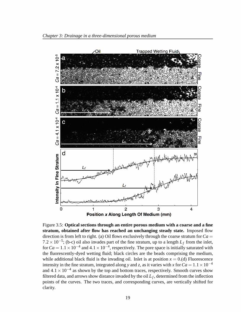
Figure 3.5:Optical sections through an entire porous medium with a coarse and a finestratum, obtained after flow has reached an unchanging steady state. Imposed flowdirection is from left to right. (a) Oil flows exclusively through the coarse stratum forCa=7.2×10⁻⁵; (b-c) oil also invades part of the fine stratum, up to a lengthL f from the inlet,for Ca= 1.1×10⁻⁴ and 4.1×10⁻⁴, respectively. The pore space is initially saturated withthe fluorescently-dyed wetting fluid; black circles are the beads comprising the medium,while additional black fluid is the invading oil. Inlet is at positionx = 0.(d) Fluorescenceintensity in the fine stratum, integrated alongy andz, as it varies withx for Ca= 1.1×10⁻⁴
and 4.1×10⁻⁴ as shown by the top and bottom traces, respectively. Smooth curves showfiltered data, and arrows show distance invaded by the oilL f , determined from the inflectionpoints of the curves. The two traces, and corresponding curves, are vertically shifted forclarity.
19

Chapter 3: Drainage in a three-dimensional porous medium
expectation is in direct agreement with the observed drainage behavior, shown in Figure
3.5(a).
An additional viscous pressure,Pv, drives the continued flow of oil through the coarse
stratum; we use Darcy’s law to estimate this asPv(x) = µo(Q/Ac)(L−x)/kc. We estimate
the permeability of the coarse stratum to the oil,kc, using the Kozeny-Carman relation
kc ≈ κ45
φ3
(1−φ)2 a2c [94]; the relative permeabilityκ quantifies the permeability reduction re-
sulting from trapping of the wetting fluid within the crevices of the medium, as visible in
Figure 3.5(a). We independently measureκ ≈ 0.16 using a homogeneous porous medium
constructed and drained in a manner similar to the experiments reported here.
We hypothesize that the oil begins to invade the fine stratum when the flow rate is
sufficiently large for the viscous pressure at the inlet,Pv(0), to balance the capillary pressure
required to invade a pore of the fine stratumPγ , f . In non-dimensional form, this criterion is
Ca≈Ca∗ ≡ 2accosθ0.16af
ac
Lκ45
φ3
(1−φ)2
Ac
A(3.1)
We therefore expect drainage through only the coarse stratum for Ca< Ca∗; for Ca above
this threshold, the oil can also begin to invade the adjacentfine stratum, in agreement
with our observations [Figure 3.5(a-c)]. To test this prediction quantitatively, we repeat
the experiments on many different stratified porous media, varying the bead sizesac and
af , medium lengthL, and the cross-sectional areasA andAc; this enables us to varyCa∗
over one order of magnitude,Ca∗ ∼ 10−5−10−4. For all of the media tested, we observe
exclusive drainage through the coarse stratum below a threshold value ofCa, while above
this threshold, the oil also begins to invade the adjacent fine stratum, as shown by the open
and filled symbols in Figure 3.6, respectively. We find that the threshold for invasion into
20
Chapter 3: Drainage in a three-dimensional porous medium
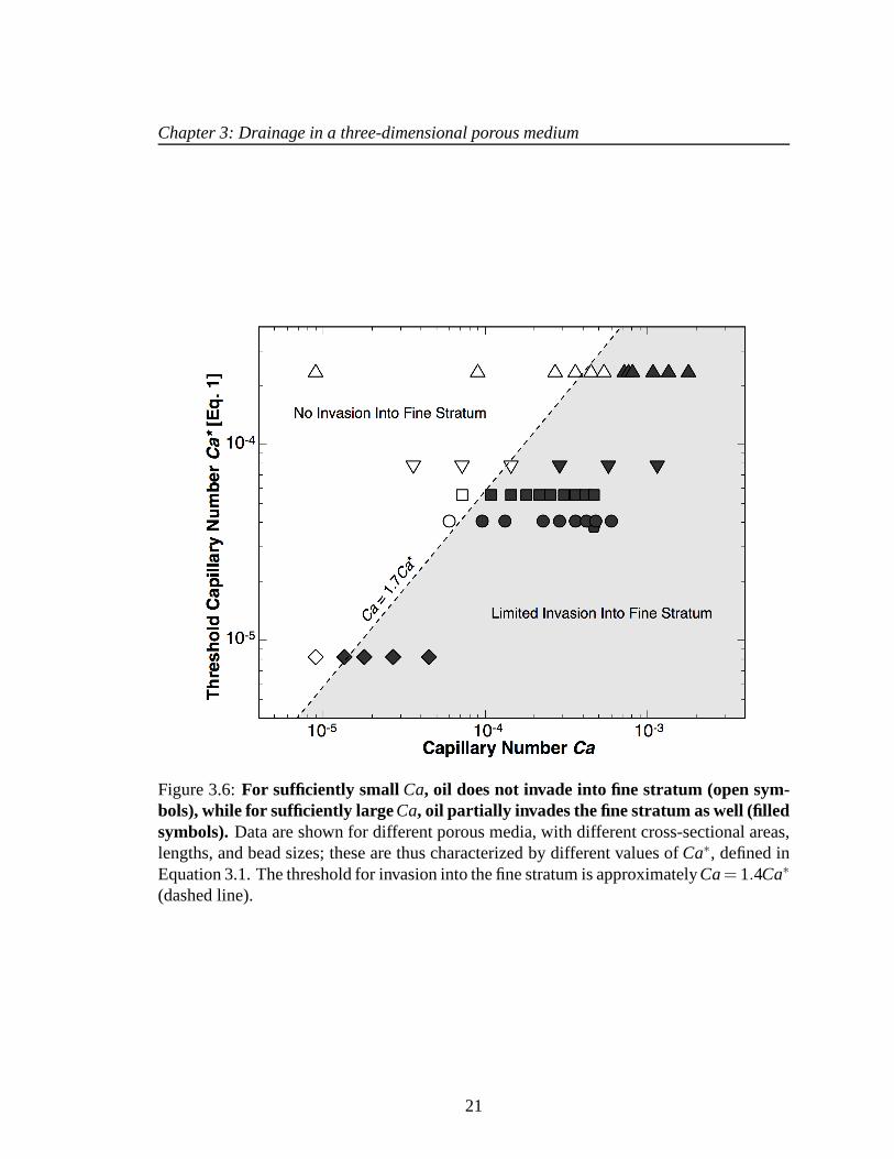
Figure 3.6:For sufficiently small Ca, oil does not invade into fine stratum (open sym-bols), while for sufficiently largeCa, oil partially invades the fine stratum as well (filledsymbols).Data are shown for different porous media, with different cross-sectional areas,lengths, and bead sizes; these are thus characterized by different values ofCa∗, defined inEquation 3.1. The threshold for invasion into the fine stratum is approximatelyCa= 1.4Ca∗
(dashed line).
21

Chapter 3: Drainage in a three-dimensional porous medium
Figure 3.7:Time sequence of confocal micrographs, taken atCa> Ca∗, showing flowof oil (black) from the coarse stratum laterally into the fine stratum, indicated byarrows in first panel. The flow is characterized byCa= 4.7×10⁻⁴ andCa∗ = 3.8×10⁻⁵.Imposed flow direction is from left to right.
the fine stratum is given byCa≈ 1.4Ca∗ over a broad range ofCa∗ [Figure 3.6, dashed
line], in close agreement with our prediction [Equation 3.1].
Within this picture, for sufficiently largeCa, oil is forced into the fine stratum not only
from the inlet, but also laterally, from the adjacent coarsestratum [137, 138, 139]. By
directly visualizing the drainage dynamics atCa > Ca∗, we confirm this lateral flow, as
indicated by the arrows in Figure 3.7. We therefore expect that the oil invades the fine
stratum for allx≤ L f , wherePv exceedsPγ , f . Balancing these pressures yields
L f /L = 1−Ca∗/Ca (3.2)
We test this prediction by measuring the variation ofL f with Ca for the different stratified
porous media, characterized byCa∗ ∼ 10−5−10−4. For all of the experiments, we find that
L f /L increases with increasingCa [inset to Figure 3.8], consistent with our expectation.
Moreover, the data for different porous media collapse whenCa is rescaled byCa∗, as
shown in Figure 3.8, in agreement with Equation 3.2. The findings presented in Figure 3.6
suggest thatCa∗ should be replaced by 1.4Ca∗ in Equation 3.2; this yields an excellent fit
22

Chapter 3: Drainage in a three-dimensional porous medium
Figure 3.8: Geometry of invasion. (Inset) Distance invadedinto the fine stratum,L f , in-creases with increasingCa; different symbols represent different media characterized bydifferent values ofCa∗. Symbols are the same as in Figure 3.L is the length of the medium.(Main panel) Data collapse whenCa is rescaled byCa∗, and agree well with the theoreticalpredictionL f /L = 1−1.4Ca∗/Ca (dashed line).
to the data, as shown by the dashed line in Figure 3.8. Our model thus captures both the
onset and the spatial extent of oil invasion into the fine stratum.
To test the generality of our results, we also study media with three different strata: a
coarse stratum, comprised of beads with radiusac = 75µm, a fine stratum, comprised of
beads with radiusaf = 19µm, and an intermediate stratum separating the two, comprised of
beads with radiusam = 38µm. We observe flow behavior similar to the case of two strata:
for Ca= 1.8×10⁻⁵ and 4.8×10⁻⁵, the oil flows through the entire coarse stratum, and also
23

Chapter 3: Drainage in a three-dimensional porous medium
Figure 3.9:Optical section through part of a porous medium with three strata, ob-tained after the flow has reached an unchanging steady state.Both coarse and inter-mediate strata are completely invaded by the oil (black), while the fine stratum is onlypartially invaded, as indicated by the arrow. Imposed flow direction is from left to right;Ca= 9.0×10⁻⁵. The thresholdCa∗ = 2.4×10⁻⁵ and 5.5×10⁻⁵ for the intermediate andfine strata, respectively.
partially invades the intermediate stratum; the spatial extent of this invasion increases with
increasingCa. Moreover, at an even higherCa= 9.6×10⁻⁵, the oil also partially invades
the fine stratum. The partial invasion into the intermediatestratum requires the lateral flow
of oil from the coarse stratum; we thus expect that, if the positions of the intermediate
and fine strata are switched, the intermediate stratum becomescompletely, not partially,
invaded above a thresholdCa. To test this idea, we study a medium with the fine stratum
separating the coarse and the intermediate strata. At aCa= 4.5×10⁻⁵, the oil completely
invades both coarse and intermediate strata, in contrast with the previous case, and in direct
agreement with our expectation [top and bottom strata in Figure 3.9]. Moreover, at an even
higherCa = 9.0× 10⁻⁵, the oil partially invades the fine stratum [arrow in Figure 3.9],
consistent with the picture presented here. These observations confirm that the flow path
taken by the oil depends not only on the geometry of the individual strata, but also on their
relative positions.
24

Chapter 3: Drainage in a three-dimensional porous medium
Using direct visualization by confocal microscopy, we demonstrate how stratification
alters the path taken by a non-wetting fluid as it drains a 3D porous medium. For sufficiently
smallCa, drainage proceeds only through the coarsest stratum of themedium; above a
thresholdCa, the non-wetting fluid is also forced laterally, into part ofthe adjacent, finer
strata. Our results highlight the essential role played by pore-scale capillary forces, which
are frequently neglected from stratum-scale models of flow,in determining this behavior.
Because geological formations are frequently stratified, we expect that our work will be
relevant to a number of important applications, including understanding oil migration [140,
141], preventing groundwater contamination [142, 143], and sub-surface storage of CO2
[144].
25

Chapter 4
Imbibition in a three-dimensional
porous medium
The previous Chapter described drainage, the displacementof a wetting fluid from a
porous medium by an immiscible non-wetting fluid. Another important class of multi-
phase flow is imbibition, the displacement of a non-wetting fluid from a porous medium
by an immiscible wetting fluid. When the 3D pore space is highly disordered, the fluid
displacement during imbibition is complex; this can lead tothe formation and trapping of
discrete ganglia of the non-wetting fluid within the porous medium [10, 11, 12, 13, 14, 15,
16, 17, 18]. Some of this trapped non-wetting fluid can become mobilized as the capil-
lary number characterizing the continued flow of the wettingfluid, Ca≡ µw(Qw/A)/γ, is
increased [145, 146, 19, 147, 148, 149]; µw is the viscosity of the wetting fluid,A is the
cross-sectional area of the medium, andγ is the interfacial tension between the two flu-
ids. The pore-scale physics underlying this phenomenon remains intensely debated. Visual
inspection of the exterior of a porous medium, as well as somesimulations, suggest that
26

Chapter 4: Imbibition in a three-dimensional porous medium
asCa increases, the ganglia are not immediately mobilized; instead, they break up into
smaller ganglia only one pore in size [150, 151]. These then remain trapped within the
medium, becoming mobilized only for largeCa. By contrast, other simulations, as well
as experiments on individual ganglia, suggest that the ganglia do not break up; instead, all
ganglia larger than a threshold size, which decreases with increasingCa, become mobilized
[86, 152, 153, 154]. The differences between these conflicting pictures, suchas the geomet-
rical configurations of the trapped ganglia, can have significant practical consequences: for
example, smaller ganglia present a higher surface area per unit volume, potentially lead-
ing to their enhanced dissolution in the wetting fluid [155, 156]. This behavior impacts
diverse situations ranging from the spreading of contaminants in groundwater aquifers to
the storage of CO2 in brine-filled formations. Elucidating the physics underlying ganglion
trapping and mobilization is thus critically important; however, despite its enormous indus-
trial relevance, a clear understanding of this phenomenon remains lacking. Unfortunately,
systematic experimental investigations of it are challenging, requiring direct measurements
of the pore-scale ganglia configurations within a 3D porous medium, as well as of the bulk
transport through it, over a broad range of flow conditions.
In this Chapter3, we use confocal microscopy to directly visualize the formation and
intricate morphologies of the trapped non-wetting fluid ganglia within a model 3D porous
medium. The ganglia vary widely in their sizes and shapes. Intriguingly, these configura-
tions do not vary for sufficiently smallCa; by contrast, asCa increases above a threshold
value≈ 2×10⁻⁴, the largest ganglia start to become mobilized from the medium. Both the
3Based on “Mobilization of a trapped non-wetting fluid from a three-dimensional porous medium”,S. S.Datta, T. S. Ramakrishnan, and D. A. Weitz, to be submitted (2013) and “Visualizing multi-phase flow andtrapped fluid configurations in a model three-dimensional porous medium”, A. T. Krummel∗, S. S. Datta∗,S. Munster, and D. A. Weitz,AIChE Journal59, 1022 (2013) *Equal contribution.
27
Chapter 4: Imbibition in a three-dimensional porous medium
size of the largest trapped ganglion, and the total amount oftrapped non-wetting fluid, de-
crease with increasingCa. We do not observe significant effects of ganglion breakup inour
experiments. By combining our 3D visualization with measurements of the bulk transport
properties of the medium, we show that the variation of the ganglia configurations withCa
can instead be understood using a mean-field model balancingthe viscous forces exerted
on the ganglia with the capillary forces that keep them trapped within the medium.
4.1 Pore-scale dynamics of secondary imbibition
To mimic discontinuous core-flood experiments on reservoirrocks, we first drain a
wetting-fluid saturated 3D porous medium with 15 pore volumes of the non-wetting oil at
a prescribed volumetric flow rateQnw = 1 mL h−1 through the porous medium. We then
flow dyed wetting fluid at a fixed volumetric flow rateQw, as schematized in Figure 4.1; this
process is known as secondary imbibition. To quantify the competition between the viscous
and capillary forces at the pore scale, we calculate the corresponding capillary number,
Ca≡ µw(Qw/A)/γ ∼ 6.4×10⁻⁷. This definition ofCa frequently occurs in the literature,
and we therefore use it in this and the previous Chapter to facilitate comparison between
our results and previous work. However, we note that a more accurate representation of
the viscous force would also incorporate the medium porosity φ : the ratio of the viscous
and capillary pressures then scales asµnw(Qnw/φA)/γ instead. We use this more accurate
definition ofCa in Chapter 6.
The presence of the thin layers of the wetting fluid profoundly changes the flow dy-
namics: unlike the case of drainage, discussed in the previous Chapter, the invading fluid
does not simply burst into the pores. Instead, we observe that the wetting fluid first flows
28

Chapter 4: Imbibition in a three-dimensional porous medium
Figure 4.1: Visualizing secondary imbibition within a 3D porous medium. (a) Schematicof experimental setup. We directly visualize the flow withinthe medium using confocalmicroscopy. The fluorescently-dyed wetting fluid displacesthe undyed non-wetting oil.(b) Optical section through part of the medium, taken as the wetting fluid displaces the oilatCa= 6.4×10⁻⁷. Section is obtained at the same fixedz position, away from the lateralboundaries of the medium, as in Figure 3.1(b-c). Bright areas show the fluorescently-dyed wetting fluid, and the black circles show cross-sections of the beads making up themedium. Additional black areas show the oil. The wetting fluid first pinches off oil increvices throughout the medium, as seen in the region spanned by the double-headed arrow,and then bursts into the pores of the medium, starting at the inlet, as seen in the regionspanned by the single-headed arrow. Some oil ganglia remaintrapped within the medium,as indicated. (c-d) Time sequence of zoomed confocal micrographs, with the oil-filled porespace subtracted; binary images thus show wetting fluid in white as it (c) initially pinchesoff oil in the crevices, and then (d) invades the pores. Time stamps indicate time elapsedafter subtracted frame. Last frame shows unchanging steadystate; arrow indicates a trappedoil ganglion. Scale bars in (b) and (c-d) are 500µm and 200µm, respectively. Imposedflow direction in all images is from left to right.
29

Chapter 4: Imbibition in a three-dimensional porous medium
Figure 4.2:Pore-scale dynamics of secondary imbibition depend strongly on Ca. Im-ages show multiple frames, taken at different times after drainage, of a single optical slice.The slice is 11µm thick and is imaged within a porous medium comprised of beads withaverage radiusa = 75 µm, with cross-sectional width 3 mm and height 1 mm. The brightareas show the dyed wetting fluid; the dark circles are the beads, while the additional darkareas are the undyed oil being displaced from the pore volume. Direction of bulk wettingfluid flow is from left to right. The final frame shows the unchanging steady state. Labelsshow time elapsed after first frame. (a) At lowCa= 7×10⁻⁶, the wetting fluid pinches offthe oil at multiple nonadjacent constrictions, then displaces the oil from the surroundingpores. The wetting fluid eventually flows through a tortuous,continuous network of filledpores, forming many trapped oil ganglia. (b) At highCa= 6×10⁻⁴, the occurrence of oilpinch-off is reduced, and the wetting fluid displaces the oilfrom the pores, leaving a fewsmall oil ganglia trapped within the medium. Scale bars are 200 µm.
30

Chapter 4: Imbibition in a three-dimensional porous medium
through the thin layers, pinching off the oil in multiple nonadjacent crevices throughout
the entire medium [112, 157, 158] over a period of approximately 60 s, as seen in the re-
gion spanned by the double-headed arrow in Figure 4.1(b), in the time sequence shown in
Figure 4.1(c), and in the time sequence shown in Figure 4.2(a). This behavior agrees with
the predictions of recent numerical simulations [159]. The wetting fluid then also begins
to invade the pores through a series of intermittent, abruptbursts, starting from the inlet,
as seen in the region spanned by the single-headed arrow in Figure 4.1(b) and in the time
sequence shown in Figure 4.1(d). Interestingly, as the wetting fluid invades the medium, it
bypasses many of the pores, leaving discrete oil ganglia of varying sizes in its wake. Many
of these ganglia remain trapped within the pore space, as indicated in Figure 4.1(b).
To explore the dependence of oil displacement on flow conditions, we visualize sec-
ondary imbibition for varyingCa. Unlike the lowCacase, we do not observe oil pinch-off
at higherCa∼ 10−4−10−3; instead, the wetting fluid displaces the oil from the pores,as
shown in Figure 4.2(b). This indicates that flow through the thin wetting layers becomes
less significant asCa is increased. This observation confirms the predictions of recent sim-
ulations [129, 125]. However, some of the oil is still bypassed by the wetting fluid, forming
disconnected oil ganglia [160]; in several cases, the ganglia break up into smaller ganglia.
Many of these ganglia are mobilized from the medium; however, a few smaller ganglia re-
main trapped [last frame in Figure 4.2(b)]. For sufficientlylong times, these ganglia cease
to move, and the pressure drop across the medium does not appreciably change, indicating
that a steady state is reached. These results thus highlightthe important role played by the
wetting layers in influencing the flow behavior.
31

Chapter 4: Imbibition in a three-dimensional porous medium
4.2 Trapped oil ganglia configurations
We use our confocal micrographs to measure the total amount of oil trapped within the
porous medium; this is quantified by the residual oil saturation, Sor ≡Vo/φV, whereVo is
the total volume of oil imaged within a region of volumeV andφ is the porosity of the
medium. After secondary imbibition atCa = 6.4×10⁻⁷, we find Sor ≈ 9%. To mimic
discontinuous core-flood experiments on reservoir rocks, we then explore the variation of
Sor in response to progressive increases in the wetting fluidCa. For each value ofCa,
we flow at least 13 pore volumes of the wetting fluid, thus establishing a new steady state,
before reacquiring an additional set of 3D stacks. By comparing each set of stacks with that
obtained during the initial pore structure characterization, we obtain the 3D morphologies
of the oil ganglia left trapped at eachCa. The Reynolds number characterizing the pore-
scale flow is given byRe≡ ρw(Qw/φA)at/µw ≈ 8× 10⁻⁶ − 8× 10⁻², whereρw is the
density of the wetting fluid,at ≈ 0.16a is the typical radius of a pore entrance, anda is
the average bead radius; our experiments are therefore characterized by laminar flow. The
Bond number characterizing the influence of gravity relative to capillary forces at the pore
scale is given byBo≡ g(ρw−ρnw)a2t /γ ≈ 10−6, whereρnw is the density of the non-wetting
fluid, indicating that gravity only becomes appreciable on the vertical length scale of the
entire medium. We therefore neglect gravity from our subsequent theoretical analysis.
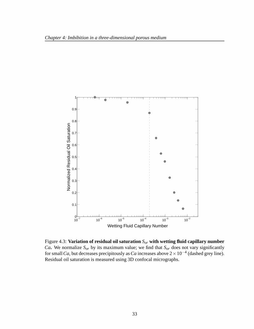
We find thatSor does not vary significantly for sufficiently smallCa; however, asCa is
increased above 2×10⁻⁴, Sor decreases precipitously, as shown in Figure 4.3, ultimately
reaching only≈ 7% of its initial value. These results are consistent with the results of
previous core-flood experiments, which show similar behavior for fluids of a broad range
of viscosities and interfacial tensions [149].
32
Chapter 4: Imbibition in a three-dimensional porous medium
10−7
10−6
10−5
10−4
10−3
10−2
0
0.1
0.2
0.3
0.4
0.5
0.6
0.7
0.8
0.9
1
Nor
mal
ized
Res
idua
l Oil
Sat
urat
ion
Wetting Fluid Capillary Number
Figure 4.3:Variation of residual oil saturation Sor with wetting fluid capillary numberCa. We normalizeSor by its maximum value; we find thatSor does not vary significantlyfor smallCa, but decreases precipitously asCa increases above 2×10⁻⁴ (dashed grey line).Residual oil saturation is measured using 3D confocal micrographs.
33

Chapter 4: Imbibition in a three-dimensional porous medium
Figure 4.4:3D renderings of oil ganglia trapped after secondary imbibition at Ca=6.4×10⁻⁷. The left ganglion is spherical and only spans≈ 0.3 beads in diameter, whereasthe right ganglion is more ramified and spans multiple beads.Renderings are producedusing 3D confocal micrographs.
To better understand this behavior, we inspect the reconstructed 3D morphologies of
the individual ganglia for eachCa investigated. At the smallestCa≈ 6×10⁻⁷−2×10⁻⁴,
the ganglia morphologies vary widely, as exemplified by the 3D renderings shown in
Figure 4.4. The smallest ganglia are spherical, only occupying single pores, and span≈ 0.3
beads in size [left, Figure 4.4]; in stark contrast, the largest ganglia are ramified, occupying
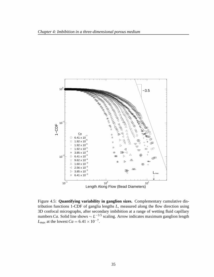
multiple pores, and span many beads in size [right, Figure 4.4]. To quantify the signifi-
cant variation in their morphologies, we measure the lengthL of each ganglion along the
flow direction, and plot 1-CDF(L), where CDF= ∑L0 Lp(L)/∑∞
0 Lp(L) is the cumulative
distribution function of ganglia lengths andp(L) is the number fraction of ganglia having
a lengthL. Consistent with the variability apparent in the 3D renderings, we find that the
ganglia lengths are broadly distributed, as indicated by the circles in Figure 4.5.
Percolation theory predicts that the number fraction of ganglia with volumes is, for
larges, given byp(s) ∝ s−τ , whereτ ≈ 2.2 is a scaling exponent [161, 162, 163]. More-
34
Chapter 4: Imbibition in a three-dimensional porous medium
10−1
100
101
10−2
10−1
100
Length Along Flow (Bead Diameters)
1−C
DF
6.41 x 101.92 x 101.92 x 101.92 x 103.85 x 106.41 x 109.62 x 101.60 x 102.56 x 103.85 x 106.41 x 10
−7
−6
−5
−4
−4
−4
−4
−3
−3
−3
−3
Ca
L
−3.5
max
Figure 4.5:Quantifying variability in ganglion sizes. Complementary cumulative dis-tribution functions 1-CDF of ganglia lengthsL, measured along the flow direction using3D confocal micrographs, after secondary imbibition at a range of wetting fluid capillarynumbersCa. Solid line shows∼ L−3.5 scaling. Arrow indicates maximum ganglion lengthLmax at the lowestCa= 6.41×10⁻⁷.
35

Chapter 4: Imbibition in a three-dimensional porous medium
over, the volume of a ganglion varies with its length ass∝ L3/(τ−1). Combining these two
relations yieldsp(L) ∝ L−3τ/(τ−1), and therefore,Lp(L) ∝ L−3τ/(τ−1)+1. In our experi-
ments, we measure the complementary cumulative distribution function of ganglia lengths,
1-CDF(L) = ∑∞L Lp(L)/∑∞
0 Lp(L). The percolation theory prediction is thus 1−CDF(L) ∝
L−3τ/(τ−1)+2 ∝ L−3.5, usingτ ≈ 2.2; this prediction is in good agreement with the largeL
tail of our data, as shown by the solid line in Figure 4.5. Thisresult also agrees with re-
cent X-ray microtomography experiments [26, 164]. We also find that the largest trapped
ganglion has a lengthLmax≈ 13 bead diameters [arrow in Figure 4,5]; while we cannot
exclude the influence of boundary effects or the limited imaging volume, this value is in
good agreement with the prediction of percolation theory, incorporating a non-zero viscous
pressure:Lmax≈ α(a2Ca/κk)−ν/(1+ν) ≈ 9α bead diameters, whereν ≈ 0.88 is a scaling
exponent,α is a constant of order unity, and we use the value ofκ measured at the lowest
Ca [165]. Taken together, these results suggest that the configurations of the ganglia left
trapped after secondary imbibition can be understood usingpercolation theory.
AsCa increases, we donotobserve significant effects of ganglia breakup; this observa-
tion is contrary to some previous suggestions [151], and confirms the predictions of other
numerical simulations [153]. Instead, the ganglia configurations remain the same for all
Ca< 2×10⁻⁴ [◦, �, and× in Figure 4.5]. Moreover, we find that the largest ganglia start
to become mobilized from the porous medium, concomitant with the observed decrease in
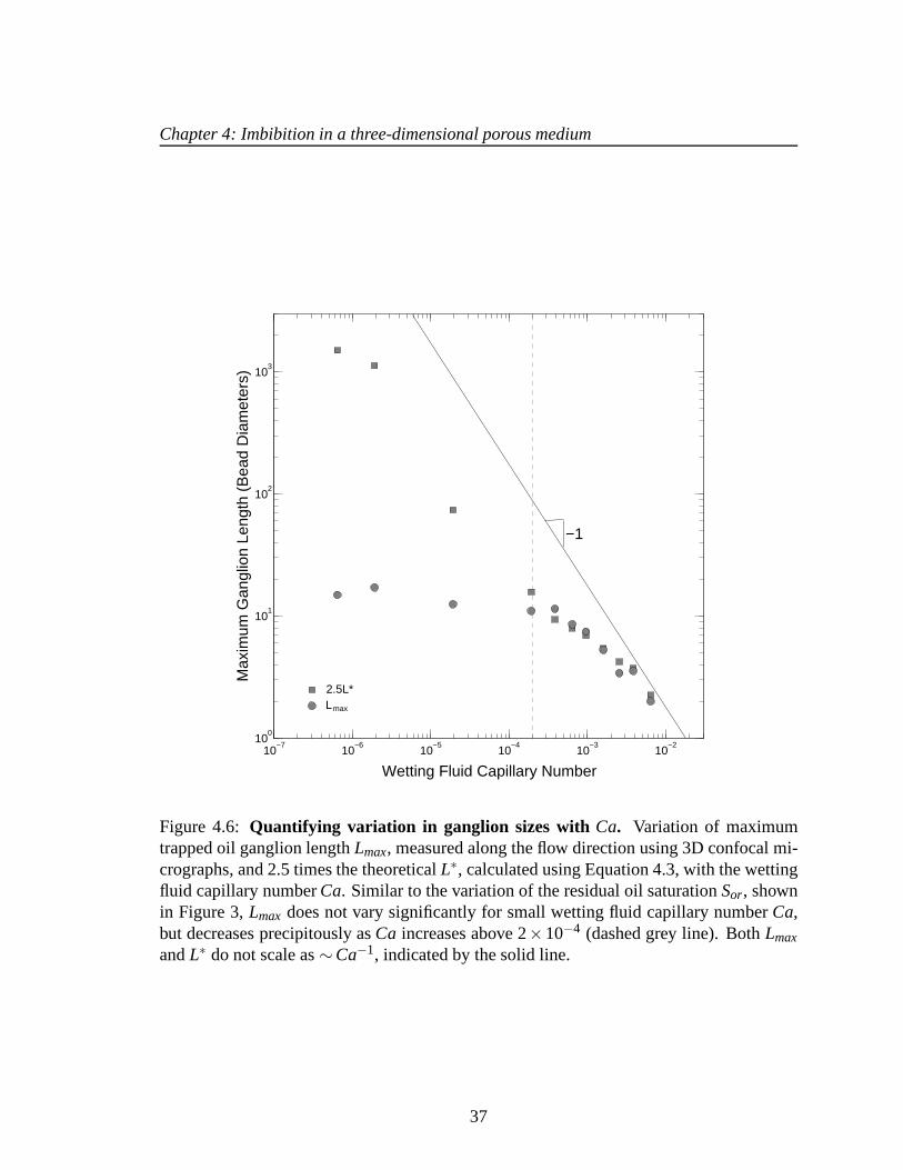
Sor, onceCa increases above 2× 10⁻⁴ [Figure 4.5]. We quantify this behavior by plot-
ting the variation ofLmax with Ca. While Lmax remains constant at smallCa, it decreases
precipitously asCa increases above 2×10⁻⁴, as shown by the circles in Figure 4.6. Re-
markably, this behavior closely mimics the observed variation of Sor with Ca [Figure 4.3].
36
Chapter 4: Imbibition in a three-dimensional porous medium
10−7
10−6
10−5
10−4
10−3
10−2
100
101
102
103
Max
imum
Gan
glio
n Le
ngth
(B
ead
Dia
met
ers)
−1
Wetting Fluid Capillary Number
2.5L*Lmax
Figure 4.6: Quantifying variation in ganglion sizes with Ca. Variation of maximumtrapped oil ganglion lengthLmax, measured along the flow direction using 3D confocal mi-crographs, and 2.5 times the theoreticalL∗, calculated using Equation 4.3, with the wettingfluid capillary numberCa. Similar to the variation of the residual oil saturationSor, shownin Figure 3,Lmax does not vary significantly for small wetting fluid capillarynumberCa,but decreases precipitously asCa increases above 2×10⁻⁴ (dashed grey line). BothLmax
andL∗ do not scale as∼Ca−1, indicated by the solid line.
37

Chapter 4: Imbibition in a three-dimensional porous medium
These results thus suggest that the variation ofSor with increasingCa is not determined by
the breakup of the trapped ganglia; instead, it may reflect the mobilization of the largest
ganglia from the medium.
4.3 Physics of ganglion mobilization
To understand the ganglia mobilization, we analyze the distribution of pressures in the
wetting fluid as it flows through the porous medium. Motivatedby previous studies of
this flow [166, 86, 19], we make the mean-field assumption that the viscous pressure drop
across a ganglion of lengthL is given by Darcy’s law,
Pv =µw
κkQw
AL (4.1)
The relative permeabilityκ ≤ 1 quantifies the modified transport through the medium due
to the presence of the trapped oil. To determinePv at eachCa investigated, we use pressure
transducers to directly measure the variation ofκ with Ca for a porous medium constructed
in a manner similar to, and following the same flow procedure as, that used for visualization
of the ganglia configurations. Interestingly,κ does not vary significantly for sufficiently
smallCa; however, asCa increases above 2×10⁻⁴, κ quickly increases, concomitant with
the observed decreased inSor, as shown in Figure 4.7. This observation suggests that the
bulk transport behavior of the medium depends strongly on the trapping of oil within it. To
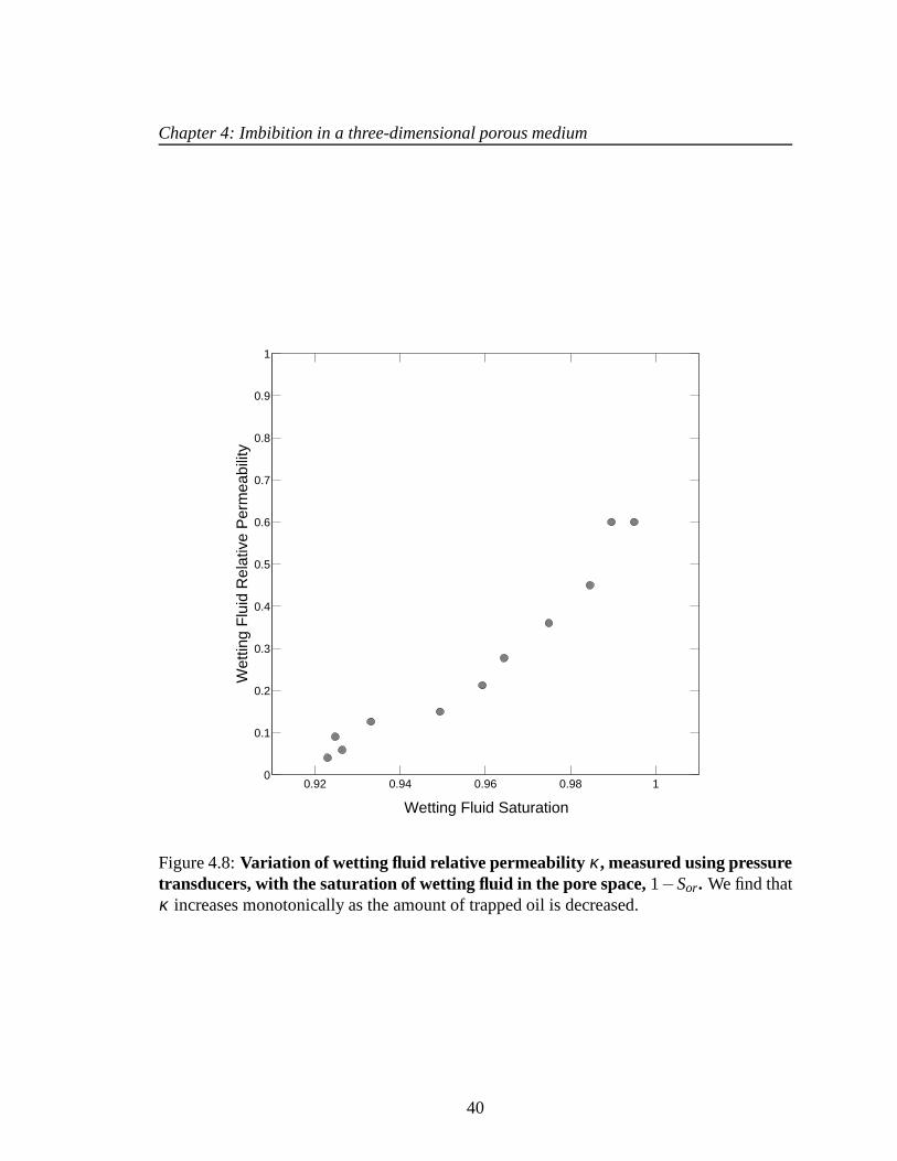
quantify the close link between the variation ofκ andSor with Ca [149], we plot κ as a
function of the wetting fluid saturation, 1−Sor. Consistent with our expectation [167], we
find thatκ increases monotonically with increasing wetting fluid saturation, as shown in
Figure 4.8.
38

Chapter 4: Imbibition in a three-dimensional porous medium
10−7
10−6
10−5
10−4
10−3
10−2
0
0.1
0.2
0.3
0.4
0.5
0.6
0.7
0.8
0.9
1
Wet
ting
Flu
id R
elat
ive
Per
mea
bilit
y
Wetting Fluid Capillary Number
Figure 4.7:Variation of wetting fluid relative permeability κ , measured using pressuretransducers, with the wetting fluid capillary number Ca. Similar to the variation ofthe residual oil saturationSor, shown in Figure 3,κ does not vary significantly for smallwetting fluid capillary numberCa; however, it increases dramatically asCa increases above2×10−4 (dashed grey line).
39
Chapter 4: Imbibition in a three-dimensional porous medium
0.92 0.94 0.96 0.98 10
0.1
0.2
0.3
0.4
0.5
0.6
0.7
0.8
0.9
1
Wet
ting
Flu
id R
elat
ive
Per
mea
bilit
y
Wetting Fluid Saturation
Figure 4.8:Variation of wetting fluid relative permeability κ , measured using pressuretransducers, with the saturation of wetting fluid in the porespace,1−Sor. We find thatκ increases monotonically as the amount of trapped oil is decreased.
40

Chapter 4: Imbibition in a three-dimensional porous medium
For a ganglion to squeeze through the pores of the medium, it must simultaneously
displace the wetting fluid from a downstream pore, and be displaced by the wetting fluid
from an upstream pore. To displace the wetting fluid from a downstream pore, a threshold
capillary pressure must build up at the pore entrance, as schematized by the right set of
arrows in Figure 4.9; this threshold is given byPt = 2γ cosθ/at , whereat is the radius of
the pore entrance [15, 97, 96], with an average value≈ 0.16a for a 3D packing of glass
beads [113, 114]. Similarly, for the trapped oil to be displaced from an upstream pore, the
capillary pressure within the pore must fall below a threshold, as schematized by the left
set of arrows in Figure 4.9; this threshold is given byPb = 2γ cosθ/ab, whereab is instead
the radius of the pore itself, with an average value≈ 0.24a [114, 113]. Thus, to mobilize a
ganglion from the porous medium, the total viscous pressuredrop across it must exceed a
capillary pressure threshold,
Pt −Pb =2γ cosθ
ab
(
ab
at−1
)
(4.2)
Balancing Equations 4.1 and 4.2, we therefore expect that, at a givenCa, the smallest
ganglia remain trapped within the medium; however, the viscous pressure in the wetting
fluid is sufficiently large to mobilize all ganglia larger than
Lmax= L∗ ≡ 2cosθCa
(
ab
at−1
)
κkab
(4.3)
To critically test this prediction, we compare the variation of bothLmax, directly measured
using confocal microscopy, andL∗, calculated using the measured values ofθ , k, andκ ,
with Ca. For smallCa, we findLmax< L∗, as shown by the first three points in Figure 4.6;
this indicates that the viscous pressure in the wetting fluidis too small to mobilize any
ganglia. Consequently,Sor does not vary significantly for this range ofCa, consistent with
41

Chapter 4: Imbibition in a three-dimensional porous medium
the measurements shown in Figure 4.3. AsCa increases,Lmax remains constant; however,
L∗ steadily decreases, eventually becoming comparable toLmax atCa≈ 2×10⁻⁴, shown
by the dashed line in Figure 4.6. Strikingly, asCa increases above this value, we find that
bothLmax andL∗ decrease in a similar manner, withLmax≈ 2.5L∗; this indicates that the
viscous pressure in the wetting fluid is sufficient to mobilize more and more of the largest
ganglia. Consequently, we expectSor to also decrease withCa in this range, in excellent
agreement with our measurements [Figure 4.3]. The similarity in the variation ofLmax and
Sor with Ca, and the close agreement between our measuredLmax and the predictedL∗ for
Ca> 2×10⁻⁴, thus confirm that the reduction inSor reflects the mobilization of the largest
ganglia.
Using confocal microscopy, we directly visualize the dynamics of secondary imbibi-
tion, as well as the intricate morphologies of the resultanttrapped non-wetting fluid ganglia,
within a 3D porous medium, at pore-scale resolution. The wetting fluid first flows through
thin layers coating the solid surfaces, pinching off the non-wetting fluid in crevices through-
out the medium. It then displaces the non-wetting fluid from the pores of the medium
through a series of intermittent, abrupt bursts, starting from the inlet, leaving ganglia of
the non-wetting fluid in its wake. These vary widely in their sizes and shapes, consis-
tent with the predictions of percolation theory. We do not observe significant effects of
ganglion breakup, contrary to some previous suggestions. Instead, for smallCa, the gan-
glia configurations do not appreciably change, while asCa is increased above a threshold
value, more and more of the largest ganglia become mobilizedfrom the medium. We em-
phasize that, due to the concomitant variation of the wetting fluid permeability withCa,
the measuredLmax doesnot decrease asCa−1 [solid line in Figure 4.6]; this is in contra-
42

Chapter 4: Imbibition in a three-dimensional porous medium
Figure 4.9:Physics of ganglion mobilization.2D schematic showing an oil ganglion (or-ange) trapped within the pore space, with wetting fluid flowing from left to right; beads areshown by white circles. Dashed lines show threshold curvatures required for the ganglionto invade the downstream pores or be displaced from the upstream pores.
43

Chapter 4: Imbibition in a three-dimensional porous medium
diction to results obtained for an isolated ganglion [86], for which the permeability is a
constant, which are often assumed to also apply to a population of many ganglia. By cou-
pling the 3D visualization and bulk transport measurement,we show that the variation of
the ganglia configurations can be understood by balancing the viscous forces exerted on
the ganglia with the pore-scale capillary forces that keep them trapped within the medium.
This work thus helps elucidate the fluid dynamics underlyingthe mobilization of a trapped
non-wetting fluid from a 3D porous medium.
Our results provide direct visualization of the multi-phase flow and the ganglia con-
figurations within a 3D porous medium; moreover, they highlight the applicability of a
mean-field picture in understanding the mobilization of thetrapped non-wetting fluid. This
work may thus help guide theoretical models or numerical simulations (e.g. [168, 169]).
Moreover, because many geophysical flows give rise to residual trapping, we expect that
our work will be relevant to a number of important applications, including enhancing oil
recovery, understanding the distribution of contaminantsin groundwater aquifers, or the
storage of CO2 in sub-surface formations.
44
Chapter 5
Spatial fluctuations of fluid velocities in
flow through a three-dimensional porous
medium
The flow of a single fluid through a 3D porous medium, when sufficiently slow, is typi-
cally modeled using Darcy’s law, which relates the pressuredrop across the entire medium
to the flow velocity, averaged over a sufficiently large length scale. However, while appeal-
ing, this simple continuum approach neglects local pore-scale variations in the flow, which
may arise as the fluid navigates the tortuous 3D pore space of the medium. Experimental
measurements using optical techniques [170, 171, 172, 173, 174, 175, 176, 177, 178, 179,
180, 181] and nuclear magnetic resonance imaging [182, 183, 28, 29, 184, 185] confirm
that the fluid speeds are broadly distributed. However, these measurements often provide
access to only one component of the velocity field, and only for the case of single-phase
flow; moreover, they typically yield limited statistics, due to the difficulty of probing the
45

Chapter 5: Spatial fluctuations of fluid velocities in flow through a three-dimensionalporous medium
flow in 3D, both at pore scale resolution and over large lengthscales. While theoretical
models and numerical simulations provide crucial additional insight [28, 29, 30, 31, 32,
33, 34, 35, 36, 37, 1, 38, 39, 40], fully describing the disordered structure of the medium
can be challenging. Consequently, despite its enormous practical importance, a complete
understanding of flow within a 3D porous medium remains elusive.
In this Chapter4, we use confocal microscopy to directly visualize the highly variable
flow within a 3D porous medium over a broad range of length scales, from the scale of in-
dividual pores to the scale of the entire medium. We find that the velocity magnitudes and
the velocity components both along and transverse to the imposed flow direction are expo-
nentially distributed, even when a second immiscible fluid is trapped within the medium.
Moreover, we find underlying pore-scale correlations in theflow, and show that these corre-
lations are determined by the geometry of the medium. The pore space is highly disordered
and complex; nevertheless, our results indicate that fluid flow through it is not completely
random.
5.1 Visualizing single-phase flow
We prepare a rigid 3D porous medium composed of beads with radii 32±2 µm, in a
thin-walled square quartz capillary of cross-sectional areaA = 9 mm2. The packing has
lengthL ≈ 8 mm and porosityφ ≈ 0.41. To visualize the single-phase flow, we formulate
the viscous wetting fluid described in Chapter 2, suspending0.01 vol% of 1µm diameter
fluorescent latex microparticles within it. Prior to each experiment, the porous medium is
4Based on “Spatial fluctuations of fluid velocities in flow through a three-dimensional porous medium”,S. S. Datta, T. S. Ramakrishnan, and D. A. Weitz,Physical Review Letters111, 064501 (2013).
46

Chapter 5: Spatial fluctuations of fluid velocities in flow through a three-dimensionalporous medium
Figure 5.1:Visualizing flow speeds within a 3D porous medium.(a) Schematic showingporous medium and imaging geometry. A portion of the 2D map ofvelocity magnitudeswithin the medium is shown for (b) single-phase flow, and (c) flow with trapped residual oil.Black circles in (b) show beads making up the medium, while additional black regions in(c) show residual oil. Scale bars are 500µm long, while color scale shows speeds rangingfrom 0 (blue) to 12q/φ (red).
evacuated under vacuum and saturated with CO2 gas, which is soluble in the tracer-laden
fluid; this procedure eliminates the formation of trapped bubbles. We then saturate the pore
space with the tracer-laden fluid, imposing a constant volumetric flow rateQ = 0.2 mL/hr;
the average interstitial velocity is thus given byq/φ ≡ (Q/A)/φ = 15 µm/s.
To directly visualize the steady-state pore-scale flow, we use a confocal microscope to
acquire a movie of 100 optical slices in thexy plane, collecting 15 slices/s, at a fixedz
position several bead diameters deep within the porous medium. Each slice is 11µm thick
along thezaxis and spans a lateral area of 912µm× 912µm in thexyplane [Figure 5.1(a)].
To visualize the flow at the scale of the entire medium, we acquire additional movies, at
the samez position, but at multiple locations in thexy plane spanning the entire width and
length of the medium. We restrict our analysis to an area several beads away from each
edge of the medium to minimize boundary effects. To reduce image noise, we threshold
47

Chapter 5: Spatial fluctuations of fluid velocities in flow through a three-dimensionalporous medium
0 3 6 9 1210
−5
10−4
10−3
10−2
10−1
100
u/(q/φ)
PD
F
−2 −1 0 1 210
−2
10−1
100
θ (radians)
−6 −3 0 3 6 9 10
−5
10−4
10−3
10−2
10−1
100
uL/(q/φ)
PD
F
−3 0 3 6u
T /(q/φ)
32µm; with oil 75µm; no oil 32µm; no oil
ba
dc
Figure 5.2:Quantifying the variability in the flow. Probability density functions of 2D (a)normalized velocity magnitudes,u/(q/φ), (b) velocity orientation angles,θ , (c) normal-ized velocity component along the imposed flow direction,uL/(q/φ), and (d) normalizedvelocity component transverse to the imposed flow direction, uT/(q/φ). Blue circles andred squares show statistics of single-phase flow through media comprised of 32µm and75 µm radius beads, respectively, while green triangles show statistics of flow through themedium comprised of 32µm radius beads, with trapped residual oil.
48

Chapter 5: Spatial fluctuations of fluid velocities in flow through a three-dimensionalporous medium
0 1 2 3 4
0.01
0.1
1
u/(q/φ)
PD
F
Entire medium
1 x 1 pores2
10 x 10 pores2
2 x 2 pores2
Figure 5.3: Dependence of statistics on window size.Probability density functions ofnormalized 2D velocity magnitudes,u/(q/φ), for single-phase flow without residual oiltrapping through a medium comprised of beads with average radius 32µm, for squarewindows approximately one (diamonds), two (crosses), and ten (stars) pores across; circlesshow data for the entire porous medium. Data are vertically offset for clarity.
and apply a median filter to each optical slice. We have verified that the results presented
do not significantly change depending on how the images are filtered. We have also verified
that the results do not change with depth (z position), for the imaging parameters used.
The ratio of viscous forces to gravitational forces on the tracer particles is given by
9µw(q/φ)/2(ρw−ρp)ga2p≈ 104−105, whereg is gravitational acceleration, andρw≈ 1.23
g cm−3 andρp ≈ 1.01 g cm−3 are the densities of the fluid and the particles, respectively;
moreover, the time required for a particle to settle a vertical distance of 11µm, equal to the
thickness of the optical slice, is< 104×11 µm/(q/φ)∼ 10 min, approximately 100 times
larger than the time required to acquire one movie. The time for a tracer particle to diffuse
its own size is approximatelyπµwa3p/kBT ≈ 6 s, wherekB is Boltzmann’s constant andT ≈
300K is temperature; this is almost 100 times larger than thetime between two successive
frames of the movies. We thus conclude that the tracer particles are faithfully advected
49

Chapter 5: Spatial fluctuations of fluid velocities in flow through a three-dimensionalporous medium
with the flow. We note that measurements in two dimensional micromodels suggest that
the tracer particles may not fully sample the smallest fluid velocities near the bead surfaces.
However, we do not expect this to significantly affect the measured distribution of the
larger fluid velocities, which are the primary focus of our work. Moreover, we do not
observe significant differences between the data for porousmedia comprised of 32µm and
75 µm beads. The tracer Peclet number, quantifying the importance of advection relative
to diffusion in determining the particle motion, is(q/φ)/(kBT/6πap) > 103; thus, our
experiments only probe the advection motion of the fluid, in contrast to other measurements
that measure the combined effects of advection and diffusion.
We use the PIVLab package for MATLAB to characterize the flow field using parti-
cle image velocimetry, dividing each optical slice into 16129 interrogation windows, and
calculating the displacement of tracer particles in each window by cross-correlating suc-
cessive slices of each movie. By combining the displacementfield thus obtained for all
the positions imaged, and dividing the displacements by thefixed time difference between
slices, we generate a map of the 2D fluid velocities,u, over the entire extent of the porous
medium. This protocol thus enables us to directly visualizethe flow field, both at the scale
of the individual pores and at the scale of the overall medium. For calibration, we use this
protocol to visualize and confirm the parabolic Poiseuille flow profile within a square cap-
illary of cross-sectional width 550µm. Moreover, we confirm that PIV performed using
interrogation windows 0.75 and 0.5 times the size of those used here yield similar results.
The flow within the porous medium is highly variable, as illustrated by the map of ve-
locity magnitudes shown in Figure 5.1(b). To quantify this behavior, we calculate the prob-
ability density functions (pdfs) of the 2D velocity magnitudes,u = |u|, velocity orientation
50

Chapter 5: Spatial fluctuations of fluid velocities in flow through a three-dimensionalporous medium
angles relative to the imposed flow direction,θ , and the velocity components both along
and transverse to the imposed flow direction,uL = ucosθ anduT = usinθ , respectively.
Consistent with the variability apparent in Figure 5.1(b),we find that both the velocity
magnitudes and orientations are broadly distributed, as shown by the blue circles in Fig-
ure 5.2(a-b). Interestingly, the pdf ofu decays nearly exponentially, with a characteristic
speed≈ 0.5q/φ , consistent with the results of recent numerical simulations [186].
The pore space is highly disordered and complex; as a result,we expect flow through it
to be random, and thus, the motion of the fluid transverse to the imposed flow direction to
be Gaussian distributed [40, 187]. As expected, the measured pdf ofuT is symmetric about
uT = 0; however, we find that it is strikingly non-Gaussian, againexhibiting an exponential
decay over nearly four decades in probability, with a characteristic speed≈ 0.25q/φ [blue
circles in Figure 5.2(d)]. The pdf ofuL similarly decays exponentially, consistent with
results from previous NMR measurements [183]; moreover, the characteristic speed along
the imposed flow direction is≈ 0.5q/φ , double the characteristic speed in the transverse
direction [blue circles in Figure 5.2(c)]. These results indicate that flow within a 3D porous
medium may, remarkably, not be completely random.
5.2 Quantifying correlations in the flow
To elucidate this behavior, we characterize the spatial structure of the flow by examining
the length scale dependence of the statistics shown in Figure 5.2. We do this by calculating
the velocity pdfs for observation windows, centered on the same pore, of different sizes.
Similar to the pdfs for the entire medium, the pdfs for windows one pore in size are broad;
however, they have a different shape, as exemplified by the diamonds in Figure 5.3. By
51
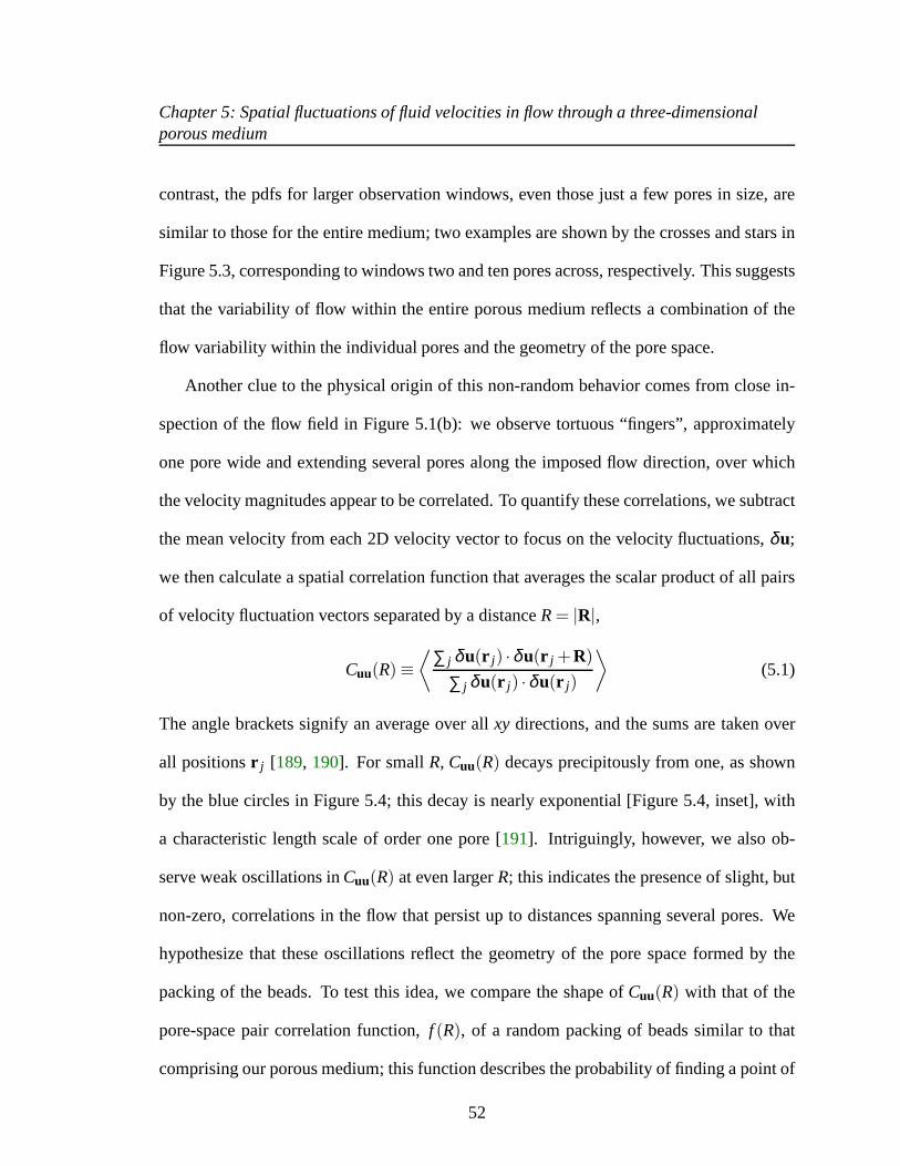
Chapter 5: Spatial fluctuations of fluid velocities in flow through a three-dimensionalporous medium
contrast, the pdfs for larger observation windows, even those just a few pores in size, are
similar to those for the entire medium; two examples are shown by the crosses and stars in
Figure 5.3, corresponding to windows two and ten pores across, respectively. This suggests
that the variability of flow within the entire porous medium reflects a combination of the
flow variability within the individual pores and the geometry of the pore space.
Another clue to the physical origin of this non-random behavior comes from close in-
spection of the flow field in Figure 5.1(b): we observe tortuous “fingers”, approximately
one pore wide and extending several pores along the imposed flow direction, over which
the velocity magnitudes appear to be correlated. To quantify these correlations, we subtract
the mean velocity from each 2D velocity vector to focus on thevelocity fluctuations,δu;
we then calculate a spatial correlation function that averages the scalar product of all pairs
of velocity fluctuation vectors separated by a distanceR= |R|,
Cuu(R) ≡⟨
∑ j δu(r j) ·δu(r j +R)
∑ j δu(r j) ·δu(r j)
⟩
(5.1)
The angle brackets signify an average over allxy directions, and the sums are taken over
all positionsr j [189, 190]. For smallR, Cuu(R) decays precipitously from one, as shown
by the blue circles in Figure 5.4; this decay is nearly exponential [Figure 5.4, inset], with
a characteristic length scale of order one pore [191]. Intriguingly, however, we also ob-
serve weak oscillations inCuu(R) at even largerR; this indicates the presence of slight, but
non-zero, correlations in the flow that persist up to distances spanning several pores. We
hypothesize that these oscillations reflect the geometry ofthe pore space formed by the
packing of the beads. To test this idea, we compare the shape of Cuu(R) with that of the
pore-space pair correlation function,f (R), of a random packing of beads similar to that
comprising our porous medium; this function describes the probability of finding a point of
52

Chapter 5: Spatial fluctuations of fluid velocities in flow through a three-dimensionalporous medium
0 0.5 1 1.5 2 2.5 3 3.5 4−0.2
0
0.2
0.4
0.6
0.8
1
R (Bead Diameters)
Cuu
, f(R
)
0 1 2 3 4
10−2
10−1
100
R (Bead Diameters)
Cuu
, f(R
)
75µm, no oil 32µm, no oil 32µm, with oil f(R)
Figure 5.4:Correlations in the flow reflect the geometry of the pore space. Variationof spatial correlation function of velocity fluctuation vectors,Cuu(R), or pore-space paircorrelation function,f (R), with distanceR. Blue circles and red squares are for single-phase flow through media comprised of 32µm and 75µm radius beads, respectively, whilegreen triangles are for flow through the medium comprised of 32 µm radius beads, withtrapped residual oil. Data forf (R) are taken from [188]. Inset shows the same data, plottedwith semilogarithmic axes. Solid arrows indicate positions of peaks inCuu atR≈ 1, 2, 2.8,and 3.7 bead diameters, while dashed arrows indicate positions of peaks inf (R) atR≈ 1.1,2, 2.7, and 3.5 bead diameters. BothCuu and f (R) show similar oscillatory behavior, withpeaks and troughs at similar locations.
53

Chapter 5: Spatial fluctuations of fluid velocities in flow through a three-dimensionalporous medium
the pore space at a distanceRaway from another point in the pore space. Similar toCuu(R),
f (R) also shows oscillations [188]; these reflect the local packing geometry of the spherical
beads [192]. Moreover, the peaks inCuu(R) occur atR≈ 1, 2, 2.8, and 3.7 bead diame-
ters, as indicated in the inset to Figure 5.4, in excellent coincidence with those observed in
f (R). This close agreement confirms that the correlations in the flow are determined by the
geometry of the pore space.
This disordered geometry forces each fluid element to followa tortuous path through
the medium, traveling a total distance larger thanL. Averaging the distances traveled by
all the fluid elements yields an effective distance traveled√
αL, whereα > 1, often re-
ferred to as the hydrodynamic tortuosity, provides an important and commonly-used mea-
sure of the variability of the flow. Acoustic [193], electrical [193], pressure [194], NMR
[195, 196, 197], and dispersion [198] measurements, as well as a theoretical calculation
[199], yield α ≈ 2 for a porous medium similar to ours. Within the picture presented here,
the distance traveled by each fluid element is approximatelyL/cos2θ ; we thus use our
measured velocity orientations [blue circles in Figure 5.2(b)] to directly calculate the tor-
tuosity. We findα = 1.80, in good agreement with the previously obtained values. This
provides additional confirmation of the validity of our picture.
To test the generality of our results, we perform similar measurements on another 3D
porous medium with beads of larger radii, 75± 4 µm. The average interstitial velocity
of the imposed flow isq/φ = 34 µm/s. Similar to the case of the smaller beads, we ob-
serve broad, exponentially-decaying velocity pdfs [red squares in Figure 5.2]; moreover,
the pdfs for both porous media collapse when the velocities are rescaled byq/φ . We again
quantify the spatial correlations in the flow using the function Cuu(R). As in the case of
54

Chapter 5: Spatial fluctuations of fluid velocities in flow through a three-dimensionalporous medium
the smaller beads,Cuu(R) decays exponentially forR< 1 bead diameter, and also exhibits
slight oscillations at even largerR, as shown by the red squares in Figure 5.4. The close
agreement between the measurements on both porous media confirms that our results are
more general.
5.3 Visualizing multi-phase flow
As described in the previous Chapter, many important situations, such as oil recov-
ery, groundwater contamination, and geological CO2 storage, involve flow around discrete
ganglia of a second, immiscible, fluid trapped within the pore space [1]. This trapping dra-
matically alters the continuum transport, presumably due to modifications in the pore scale
flow [200, 201]. However, investigations of this behavior are woefully lacking; scattering
of light from the ganglia surfaces typically precludes direct visualization of the tracer-laden
fluid flow around them. We overcome this challenge by formulating a second non-wetting
fluid composed of a mixture of hydrocarbon oils, as describedin Chapter 2. To trap residual
ganglia of the oil, we flow it for 30 min at a rate of 10 mL/hr through the porous medium
comprised of the smaller beads; we then reflow the tracer-laden fluid at a rate of 0.1 mL/hr,
corresponding to a capillary numberCa≡ µq/γ ≈ 10−5, whereγ ≈ 13 mN/m is the interfa-
cial tension between the two fluids. This protocol leads to the formation of discrete ganglia
that remain trapped within the pore space, as described in Chapter 4; the ganglia are indi-
cated in Figure 5.1(c) [149]. The tracer-laden fluid continues to flow around these ganglia;
we directly visualize this steady-state flow using confocalmicroscopy, re-acquiring movies
of optical sections at the same positions as those obtained prior to oil trapping.
Similar to the previous case without residual trapping, theflow is highly variable, as
55

Chapter 5: Spatial fluctuations of fluid velocities in flow through a three-dimensionalporous medium
illustrated by the map of velocity magnitudes shown in Figure 5.1(c). Because the gan-
glia occlude some of the pore space, the characteristic speed of the tracer-laden fluid is
larger,≈ 1.2q/φ [green triangles in Figure 5.2(a)]; moreover, because the tracer-laden
fluid must flow around the ganglia, more velocities are oriented transverse to the flow di-
rection [green triangles in Figure 5.2(b)]. As in the case without residual trapping, we
observe broad, exponentially-decaying pdfs for the velocity components [green triangles in
Figure 5.2(c-d)]; however, these pdfs are significantly broader, indicating that residual trap-
ping introduces additional variability to flow within a 3D porous medium. We again use
the measured velocity orientations [green triangles in Figure 5.2(b)] to directly calculate
the tortuosity,α. Consistent with previous indirect measurements [202], we findα = 2.24,
higher than the tortuosity measured in the previous case of single-phase flow; this further
reflects the additional flow variability introduced by residual trapping.
We quantify the spatial correlations in this flow using the functionCuu(R). Interestingly,
as in the previous case without residual trapping,Cuu(R) decays exponentially forR< 1
bead diameter, also exhibiting slight oscillations for even largerR at the same positions, as
shown by the green triangles in Figure 5.4. This indicates that the flow remains correlated,
even when a second immiscible fluid is trapped within the medium; moreover, the structure
of these correlations is again determined by the geometry ofthe pore space.
Our measurements quantify the strong velocity variations in single- and multi-phase
flow within a 3D porous medium. We find that the velocity magnitudes and the velocity
components both along and transverse to the imposed flow direction are exponentially dis-
tributed. Moreover, we present direct evidence that the flowis correlated at the pore scale,
and that the structure of these correlations is determined by the geometry of the medium.
56

Chapter 5: Spatial fluctuations of fluid velocities in flow through a three-dimensionalporous medium
The pore space is highly disordered and complex; nevertheless, our results suggest that
flow through it is not completely random.
Finally, we note that our measurements of the velocity field within a porous medium
may provide a way to predict the mechanical dispersion of molecules dissolved in the
flowing fluid; an important example of such a solute is a contaminant that dissolves in
a groundwater aquifer. Due to the strong variability in the flow velocities, as the solute
molecules are advected along with the fluid, they spread out [1].
57
Chapter 6
Fluid breakup during simultaneous
two-phase flow through a
three-dimensional porous medium
In Chapters 3 and 4, we describe one important class of multi-phase flows: forcing one
fluid to displace another immiscible fluid from a 3D porous medium. Another important
class of multi-phase flows involves thesimultaneousflow of both a wetting and a non-
wetting fluid through the tortuous 3D pore space of the medium. Due to the interfacial
tension between the two fluids, they are typically thought toflow through distinct, un-
changing, connected pathways [203, 204]; indeed, this idea underlies the interpretation of
many multi-phase transport measurements [205]. However, the validity of this assumption
remains intensely debated. Experimental measurements on a2D porous medium suggest
that, in some cases, the non-wetting fluid may not simply flow through a connected path-
way; instead, it can break up into discrete ganglia, often assmall as one pore in size, which
58

Chapter 6: Fluid breakup during simultaneous two-phase flowthrough athree-dimensional porous medium
are then advected through the medium by the flowing wetting fluid [206, 207, 208, 209].
However, the pore space of a 2D medium is considerably less connected than that of a 3D
medium [20]; this enhances the propensity of the non-wetting fluid to break up in the 2D
case [210], and thus, the applicability of such measurements to 3D porous media is unclear.
Unfortunately, probing the flow in 3D, at pore-scale resolution, is enormously challenging,
due to the opacity of the medium. Consequently, despite its enormous practical importance,
a complete understanding of the physics underlying simultaneous two-phase flow through
a 3D porous medium remains elusive.
In this Chapter5, we use confocal microscopy to directly visualize the simultaneous
flow of both a wetting and a non-wetting fluid through a 3D porous medium, at pore-scale
resolution. For small flow rates, both fluids flow through unchanging, distinct, connected
3D pathways. At higher flow rates, however, the non-wetting fluid continually breaks up
into discrete ganglia; these are then advected through the medium. We find that the tran-
sition between connected flow and breakup of the non-wettingfluid is characterized by
a state diagram that depends on the capillary numbers of boththe wetting and the non-
wetting fluids,Caw andCanw, respectively; these parameters describe the magnitude ofthe
viscous forces exerted by the wetting and the non-wetting fluids, respectively, compared to
capillary forces. Our results thus reveal and help elucidate the diversity of behavior that
arises in two-phase flow through a 3D porous medium.
5Based on “Fluid breakup during simultaneous two-phase flow through a three-dimensional porousmedium”,S. S. Datta, J. B. Dupin, and D. A. Weitz, to be submitted (2013).
59

Chapter 6: Fluid breakup during simultaneous two-phase flowthrough athree-dimensional porous medium
6.1 Visualizing multi-phase flow
We prepare a 3D porous medium composed of beads with radiia = 36±2 µm, in a
thin-walled square quartz capillary of cross-sectional areaA = 9 mm2; the typical radius
of a pore is thusap ≈ 6 µm [113, 114]. The packing has lengthL ≈ 2 cm and porosity
φ ≈ 0.41. We use the non-wetting fluid and the low-viscosity wetting fluid described in
Chapter 2 in our experiments.
We first evacuate the porous medium under vacuum and saturateit with CO2 gas, which
is soluble in the wetting fluid, thereby eliminating the formation of trapped bubbles. We
then saturate the pore space with the dyed wetting fluid, and first visualize the pore structure
within the 3D medium using a confocal microscope. We do this by acquiring optical slices
at a fixedz position several bead diameters deep within the medium; each slice is 11µm
thick along thez axis and spans a lateral area of 912µm × 912 µm in thexy plane. We
repeatedly acquire slices at multiple locations in thexyplane spanning the entire width and
length of the medium; by combining these, we obtain a map of the pore structure over the
entire extent of the porous medium. We identify the glass beads by their contrast with the
dyed wetting fluid.
To investigate the multi-phase flow, we simultaneously flow both the wetting fluid and
the oil at independently-controlled volumetric flow rates,Qw = 0.2 mL h−1 andQnw = 5.0
mL h−1, respectively; the experimental geometry is schematized in Figure 6.1(a) and Fig-
ure 6.2. Because the oil is undyed, we identify it by its additional contrast with the dyed
wetting fluid in the imaged pore space. The oil initially flowsinto the medium through a
series of abrupt bursts into the pores, remaining connectedas it flows; this behavior indi-
cates that a threshold capillary pressure∼ γ/ap must build up in the oil before it can invade
60

Chapter 6: Fluid breakup during simultaneous two-phase flowthrough athree-dimensional porous medium
Figure 6.1: Connected flow at low flow rates during simultaneous two-phase flowthrough a 3D porous medium. (a) Schematic showing porous medium and imaging ge-ometry. The oil flows at a rateQnw through a circular tube inserted coaxially in a largersquare quartz capillary, whereas the wetting fluid flows at a rateQw through the intersti-tial space between the circular tube and the square capillary. A portion of a 2D confocalsection within the medium is shown for (b)Qw = 0.2 mL h−1 andQnw = 5.0 mL h−1, and(c) Qw = 50.0 mL h−1 andQnw = 5.0 mL h−1. Black circles show beads making up themedium, while additional black regions show a section through the flowing oil. Scale baris 500µm long. The oil flows through an unchanging, tortuous, connected 3D pathway inboth cases; an example of a 3D reconstruction is shown in Figure 6.3. The imposed flowdirection is from left to right.
61

Chapter 6: Fluid breakup during simultaneous two-phase flowthrough athree-dimensional porous medium
Figure 6.2: Schematic showing inlet geometry used in the experiments.The non-wetting fluids flows through a tube inserted coaxially in the quartz capillary, while thewetting fluid flows in the crevices between the tube and the quartz capillary.
a pore. Because the packing of the beads is disordered, the path taken by the oil is tortuous;
once it traverses the entire medium, the oil continues to flowthrough this unchanging, con-
nected 3D pathway, as exemplified in Figures 6.1(b) and 6.3. We verify that the oil flows
through this pathway by monitoring its ejection at the outlet of the porous medium.
To further explore the two-phase flow, we progressively increase the wetting fluid flow
rate. ForQw < 125.0 mL h−1, the oil slightly reconfigures its flow path each timeQw is
changed [Figure 6.1 (b-c)]; it then continues to flow throughthis connected 3D pathway.
We observe dramatically different behavior at even larger flow rates: instead of simply
flowing through a connected 3D pathway, the oil continually breaks up into discrete gan-
glia, several pores in size, as shown in Figure 6.4(a). The ganglia are then advected through
the pore space by the flowing wetting fluid. This is a dynamic process [206, 207]: the oil
ganglia continually break up and coalesce, temporarily becoming immobilized at some
62

Chapter 6: Fluid breakup during simultaneous two-phase flowthrough athree-dimensional porous medium
Figure 6.3:3D reconstruction of tortuous, connected oil pathway, during simultaneousflow of oil and a wetting fluid through a 3D porous medium. The beads are not shownfor clarity; the red shows the oil as it flows through the pore space. Perspective is lookingalong the+x direction.
63
Chapter 6: Fluid breakup during simultaneous two-phase flowthrough athree-dimensional porous medium
pore entrances and eventually being pushed through others,ultimately becoming mobi-
lized from the medium. These observations contradict the idea that the oil flows through
an unchanging, connected pathway [203, 204, 205].
We next investigate the influence of increasing the oil flow rate. We progressively in-
creaseQnw, starting at 0.2 mL h−1, fixing the wetting fluid flow rate atQw = 25.0 mL h−1.
The oil again flows through an unchanging, connected 3D pathway, similar to those shown
in Figures 6.1(b-c) and 6.3. Similar to the increasingQw case, the oil slightly reconfigures
its flow path each timeQnw is changed; it then continues to flow through this connected 3D
pathway. Intriguingly, atQnw = 5.0 mL h−1, sections of this connected 3D pathway inter-
mittently break up into discrete ganglia, several pores in size. At even higher flow rates, we
again observe that the oil continually breaks up into discrete ganglia, as shown in Figure
6.4(b). Similar to the breakup observed in the case of increasing Qw, these ganglia are
advected through the pore space by the flowing wetting fluid, and are ultimately mobilized
from the medium. Our experiments thus demonstrate that, forsufficiently large fluid flow
rates, the two fluids donot flow through distinct, unchanging, connected 3D pathways, as
is often assumed [203, 204, 205]; instead, we observe a transition to a state in which the oil
is continuously broken up into discrete ganglia.
6.2 Understanding the fluid breakup
The first class of connected-to-broken up transition occursfor increasingQw. We ob-
serve that, as the oil flows into the porous medium, it is quickly broken up into large gan-
glia, many pores in size; a representative example is shown in the first frame of Figure
6.4(a). The wetting fluid pushes part of this ganglion forward [arrows, first two frames of
64

Chapter 6: Fluid breakup during simultaneous two-phase flowthrough athree-dimensional porous medium
Figure 6.4: Oil breaks up for sufficiently large flow rates during simultaneous two-phase flow through a 3D porous medium.Images show multiple frames, taken at dif-ferent times, of a single optical slice, with the beads and the pore space subtracted; thus,the dark regions in each frame only show the oil as it flows. Theimposed flow directionis from left to right. (a) AtQw = 125.0 mL h−1 andQnw = 5.0 mL h−1, the wetting fluidbreaks the oil up into smaller, discrete ganglia. (b) AtQw = 50.0 mL h−1 andQnw = 25.0mL h−1, the oil breaks up as it flows around the beads forming the porous medium. Labelsshow time elapsed after first frame. Scale bars are 50µm long.
65
Chapter 6: Fluid breakup during simultaneous two-phase flowthrough athree-dimensional porous medium
Figure 6.4(a)], ultimately breaking it off. This process forms additional, smaller ganglia
[arrows, third frame of Figure 6.4(a)]. The ganglia are eventually advected through the
pore space by the flowing wetting fluid [arrows, last two frames of Figure 6.4(a)]. This
behavior is reminiscent of drop formation in a microfluidic channel [211, 212], in which
the viscous drag exerted by a flowing wetting fluid tears discrete drops off a coflowing oil
stream. Moreover, similar to the case of drop formation, we observe that the size of the oil
ganglia formed decreases with increasingQw. We thus hypothesize that a similar mech-
anism drives this connected-to-broken up transition. We estimate the pore-scale viscous
drag force as∼ µwqwap, whereqw ≡ Qw/φA is the average interstitial velocity in the case
of single-phase wetting fluid flow. The oil breakup is resisted by the capillary force∼ γap;
balancing these two forces yields a criterion for breakup,Caw ≡ µwqw/γ ≥ Ca∗w, where
Ca∗w is a threshold capillary number. We thus expect the oil to break up at sufficiently large
values ofCaw, consistent with our experimental observations.
The second class of connected-to-broken up transition occurs for increasingQnw. This
transition is particularly counterintuitive: increasingthe flow rate of a non-wetting fluid in
a coflowing stream typicallyimpedesits breakup into drops [211, 213, 212]. A clue to the
physical origin of this transition comes from close inspection of the oil breakup process;
a representative example is shown in Figure 6.4(b). As the oil flows, it collides with a
bead making up the porous medium, indicated by the blue arrowin the first two frames of
Figure 6.4(b). It then flows around the entire bead, breakingup into two smaller ganglia
in the process [leftmost red arrows, second frame of Figure 6.4(b)]. These smaller ganglia
continue to be advected through the pore space by the flowing wetting fluid [arrows, last
three frames of Figure 6.4(b)]. This behavior is reminiscent of the breakup of a non-wetting
66

Chapter 6: Fluid breakup during simultaneous two-phase flowthrough athree-dimensional porous medium
fluid as it flows past an obstacle in a microfluidic channel [214, 215]; in such a situation,
for small fluid flow rates, the capillary force causes the non-wetting fluid to squeeze into
one the gaps around the obstacle, moving past it with breaking. By contrast, at sufficiently
large flow rates, the viscous force driving the flow of the non-wetting fluid causes it to flow
around the entire obstacle, and the fluid breaks up in the process. We hypothesize that
a similar mechanism drives this connected-to-broken up transition. We estimate the pore-
scale viscous force driving the oil flow as∼ µnwqnwap, whereqnw≡ Qnw/φA is the average
interstitial velocity in the case of single-phase oil fluid flow. The pore-scale capillary force
is again given by∼ γap; balancing these two forces yields another criterion for breakup,
Canw ≡ µnwqnw/γ ≥ Ca∗nw, whereCa∗nw is a threshold capillary number. We thus expect
the oil to break up at sufficiently large values ofCanw, consistent with our experimental
observations.
6.3 State diagram for the connected-to-broken up transi-
tion
Within the picture presented here, the breakup of the oil occurs for sufficiently large
values of the wetting fluid and non-wetting fluid capillary numbers,Caw andCanw, respec-
tively. To rigorously test this hypothesis, we perform similar measurements over a broad
range of flow rates ranging from 0.2-250.0 mL h−1, using different fluids characterized by
viscosities ranging from 2-110 mPa s, on different 3D porousmedia characterized by cross-
sectional areas ranging from 4-9 mm2 and bead radii ranging from 36-60µm; we thus vary
the capillary numbers over the rangeCaw ∼ 10−6−10−1 andCanw ∼ 10−5− 10−1. We
67
Chapter 6: Fluid breakup during simultaneous two-phase flowthrough athree-dimensional porous medium
summarize our observations using the state diagram shown inFigure 6.5. In all cases, we
observe that the oil flows through an unchanging, connected 3D pathway for small values
of Caw andCanw, shown by the unfilled symbols in Figure 6.5; however, as eitherCaw or
Canw increase, this pathway begins to intermittently break up, shown by the grey symbols
in Figure 6.5. At the largest values ofCaw or Canw, the oil continually breaks up into dis-
crete ganglia, as shown by the black symbols in Figure 6.5. All the data appear to collapse,
supporting the validity of our picture.
The first class of connected-to-broken up transition occurswhenCaw exceeds a thresh-
old value,Ca∗w; we use our measurements to estimate this value,Ca∗w = 7×10⁻⁴. Inter-
estingly, this value is much smaller than the threshold for drop formation in a microfluidic
channel,Ca∗w ∼ 1. We speculate that this difference reflects the disorderedpacking of the
beads. Indeed, direct visualization using confocal microscopy shows that, even in the case
of single-phase flow, the velocity of the flowing wetting fluidcan be over an order of mag-
nitude larger thanqw, due to the tortuosity of the pore space [216]. In our experiments,
the co-flowing oil phase occupies a large portion of the pore space, imparting even more
variability to the wetting fluid flow. We thus expect that the pore-scale viscous drag forces
can be significantly larger than the value we use in our simpleestimate,µwqwa; this leads
to a corresponding reduction inCa∗w.
The second class of connected-to-broken up transition occurs whenCanw exceeds a
threshold value,Ca∗nw; we use our measurements to estimate this value,Ca∗nw = 5×10⁻³.
Interestingly, this value is comparable to the threshold for the breakup of a non-wetting
fluid as it flows around an obstacle in a microfluidic channel [214, 215].
Motivated by the collapse of the data in Figure 6.5, we suggest that the connected-
68

Chapter 6: Fluid breakup during simultaneous two-phase flowthrough athree-dimensional porous medium
10−6
10−5
10−4
10−3
10−210
−5
10−4
10−3
10−2
Wetting Fluid Capillary Number Caw
Non
−W
ettin
g F
luid
Cap
illar
y N
umbe
r C
a nw
Figure 6.5:State diagram of the connected-to-broken up transition forsimultaneoustwo-phase flow through a 3D porous medium as a function ofCaw and Canw. Opensymbols represent flow of the non-wetting fluid through a connected 3D pathway, grey sym-bols represent intermittent breakup of this pathway, and black symbols represent continualbreakup of the oil into discrete ganglia, which are advectedthrough the pore space. Eachsymbol shape represents a different viscosity, bead size, or porous medium cross-sectionalarea. Circles:µw = 110.0 mPa s,a = 36 µm, A = 9 mm2. Squares:µw = 2.7 mPa s,a = 36 µm, A = 9 mm2. Upward triangles:µw = 110.0 mPa s,a = 36 µm, A = 4 mm2.Diamonds:µw = 2.7 mPa s,a= 36µm, A= 4 mm2. Downward triangles:µw = 2.7 mPa s,a = 60 µm, A = 9 mm2.
69

Chapter 6: Fluid breakup during simultaneous two-phase flowthrough athree-dimensional porous medium
to-broken up transition occurs when the sum of the viscous forces exerted on the flow-
ing oil exceeds capillary forces at the pore scale; this can be summarized asCaw/Ca∗w +
Canw/Ca∗nw∼ 1. We find good agreement between this relation and our experimental mea-
surements, as shown by the curve in Figure 6.5. This further supports the validity of the
picture presented here.
Our measurements reveal and help clarify the rich behavior that arises when both a
wetting and a non-wetting fluid are forced to flow through the pore space simultaneously.
Using direct visualization by confocal microscopy, we showthat, for sufficiently low fluid
flow rates, both fluids flow via distinct, unchanging, connected 3D pathways through the
medium, as is typically assumed. At sufficiently large flow rates, however, the non-wetting
fluid is continuously broken up into discrete ganglia, whichare then advected through the
pore space by the wetting fluid. We suggest that this transition occurs when the viscous
forces exerted on the flowing non-wetting fluid exceed capillary forces at the pore scale.
Such a transition may arise in multi-phase transport measurements, which are often per-
formed at capillary numbers comparable to those explored here [203, 204, 217, 218].
70

Chapter 7
Rheology of emulsions
Emulsions are suspensions of droplets of one immiscible fluid in another. They are
widely used in technological applications requiring the transport and flow of the dispersed
fluid; these include oil recovery, food products, pharmacology, coatings, and cosmetics.
The droplets are typically stabilized by a surfactant adsorbed on their interfaces; this en-
sures that there is a short-range repulsive interaction between them, which prevents their
coalescence. Such a repulsive emulsion becomes a disordered elastic solid as it is com-
pressed: this behavior can be characterized by the complex shear modulus,G∗(ω) =
G′(ω)+ iG′′(ω), whereG′ is the storage modulus,G′′ is the loss modulus, andω is the
angular frequency. For droplet volume fractions,φ , approaching random close packing of
spheres,φRCP≈0.64, from below, a repulsive emulsion exhibits a weak elasticity that arises
from thermal fluctuations [219]. By contrast, ifφ is increased aboveφRCP, the droplets are
forced to deform; as a result, the elasticity is determined by the Laplace pressure scale of
the droplets,σ/a, whereσ is the interfacial tension between the dispersed and continu-
ous phases anda is the average droplet size [219]. Even though it can act as an elastic
71
Chapter 7: Rheology of emulsions
solid, such an emulsion can nevertheless be made to flow quiteeasily: the imposition of
sufficiently large shear causes it to yield. This behavior can be elucidated using oscilla-
tory measurements ofG′ andG′′ performed at constantω and varying maximum strain
amplitudeγ. The viscoelastic moduli of a repulsive emulsion aboveφRCP become strain-
dependent for sufficiently largeγ as the emulsion yields. For increasingγ, the nonlinearG′′
exhibits a single, well-defined peak at a strainγ∗r before falling asγ−ν ′′r ; G′ concomitantly
decreases asγ−ν ′r with ν ′′
r ≈ ν ′r/2 [219, 220, 221]. The pronounced peak inG′′ is a charac-
teristic feature of soft glassy materials; it is a direct consequence of a structural relaxation
process and thus provides an effective way to characterize yielding [221]. This approach
is particularly useful for repulsive emulsions aboveφRCP, for which the peak inG′′ reflects
the irreversible rearrangements of the densely-packed droplets [220, 222].
Another widely-encountered class of emulsions is characterized by droplets with addi-
tional attractive interactions between them. In stark contrast to the repulsive case, such an
attractive emulsion can form an elastic solid even forφ well belowφRCP [223]; the bonds
between droplets result in a connected network of aggregates that can support a shear stress
[223, 224, 225, 226]. As a result, an attractive emulsion must exhibit different flow and
yielding behavior [227]. However, despite its broad industrial applications, exactly how
this behavior occurs is unknown. Thus, measurements of the characteristicγ-dependent
yielding of attractive emulsions are essential to elucidate how emulsion rheology depends
on interdroplet interactions.
In this Chapter6, we explore the rheology of attractive emulsions using oscillatory mea-
surements over a range ofφ . For increasingγ, G′′(γ) of attractive emulsions belowφRCP
6Based on “Rheology of attractive emulsions”,S. S. Datta, D. D. Gerrard, T. S. Rhodes, T. G. Mason,and D. A. Weitz,Physical Review E, 84, 041404 (2011).
72

Chapter 7: Rheology of emulsions
exhibits a single peak at a strainγ∗1 ≪ γ∗r that increases withφ . By contrast,G′′(γ) of attrac-
tive emulsions aboveφRCP exhibits two peaks atγ∗1 andγ∗2 ≈ γ∗r , unlike the repulsive case;
these reflect two distinct structural relaxation processes. The time scales of both of these
processes vary with shear rate asγ−ν with ν ≈ 0.8−1. Our results provide insight into
the elasticity and yielding of attractive emulsions and highlight the sensitivity of emulsion
rheology to attractive interactions.
7.1 Formulation of emulsions
We use emulsions comprised of silicone oil droplets dispersed in formamide, a sol-
vent with negligible evaporation; the droplets are sterically stabilized by Pluronic P105, a
non-ionic amphiphilic copolymer [228]. The mechanical measurements are performed at
T = 23◦C on strain- or stress-controlled rheometers (TA ARES G2 or Anton Paar Physica
MCR 501, respectively) using a parallel-plate geometry. The sample environment is con-
trolled using a solvent trap. The plates are roughened to eliminate wall-slip, and we verify
that measurements are independent of the gap size; furthermore, the results are similar to
those obtained using a cone-and-plate geometry, indicating that they are not significantly
influenced by the non-uniform strain field characteristic ofa parallel-plate geometry. We
pre-shear the samples prior to each measurement by imposinga 50s−1 constant shear-rate
flow for 30s, followed by oscillatory shear ofγ decreasing from 300% to 0.01% over a
period of 230s. We do not observe sample creaming over the measurement duration.
At the temperature and concentrations used here, P105 formsfreely-dispersed globular
micelles in formamide with radiusam = 6.5nm, aggregation numberνm = 31 and criti-
cal micelle concentrationc∗ = 20.2mM [229]. These micelles induce attractive depletion
73

Chapter 7: Rheology of emulsions
interactions between emulsion droplets [230], whose magnitude at interdroplet contactU
we calculate using the Vrij model [231]: U/kBT = 4πaa2mNA(c− c∗)/νm, wherea is the
average droplet radius,c is the P105 concentration,kB is Boltzmann’s constant,T is tem-
perature, andNA is Avogadro’s number. These interactions preserve a lubricating layer of
formamide between the droplets, and hence are pairwise centrosymmetric and do not resist
bending. Because ions do not appreciably self-dissociate in formamide, and because we
use a non-ionic surfactant, we do not expect electrostaticsto play a significant role [232].
To investigate the influence of attraction on the rheology ofemulsions, we prepare re-
pulsive emulsions withU = 0 (c= 7mM < c∗) and attractive emulsions withU = 7−9kBT
(c= 26.8−28.7mM) over a range ofφ using high-shear rate homogenization or sonication
with a probe tip. We densify the emulsions using centrifugation and verify that they are
stable against coalescence and Ostwald ripening [233]. We measureσ = 6−9mN/m using
a du Nouy ring. The oil volume fractionφ is determined by measuring the masses of all
components making up a sample. The droplets havea = 100,106, or 128nm and relatively
low polydispersity∼ 30−35% as measured using dynamic light scattering. We also ac-
count for the thicknesst of the surfactant layer adsorbed at the droplet surfaces to obtain
the effective volume fractionφe f f ≈ φ(1+ t/(a− t))3. We estimatet ≈ 3.1nm based on
neutron scattering data [229, 228] and further verify this by fitting viscosity measurements
of dilute repulsive samples to simulation data appropriatefor emulsions [220, 234]. This
estimate fort is likely to be unchanged even at the highestφ studied: the pressure required
to compress the surfactant layer∼ kBT/s3, whereπs2 is the interfacial area per polymer
molecule, is approximately two orders of magnitude larger than the maximum osmotic
pressure exerted on the droplets∼ 0.1σ/a [235, 219].
74

Chapter 7: Rheology of emulsions
To test the generality of our results, we also study siliconeoil-in-water emulsions sta-
bilized by an ionic surfactant, SDS. All of the data presented in this Chapter are for the
oil-in-formamide emulsions stabilized by P105, with the exception of Figures 7.7 and
7.8, which present data for the oil-in-water emulsions stabilized by SDS. These are well-
defined and stable model systems characterized by very weak (< 1kBT) or strong (> 1kBT)
attractive interdroplet interactions using an SDS concentration only slightly greater than
or significantly greater than the critical micelle concentration (c∗ ≈ 8mM), respectively
[230, 219, 236]. We prepare the emulsions using depletion fractionation;the droplets have
a = 250nm and have low polydispersity∼ 10%. To investigate the influence of attraction
on the rheology of emulsions, we study repulsive emulsions with U < 1kBT (c = 10mM)
and attractive emulsions withU ≈ 21kBT (c= 200mM). The effective volume fractionφe f f
is defined to incorporate the effects of the thin liquid film between adjacent droplets due to
their electrostatic repulsion. We study the emulsions using oscillatory rheology on a strain-
controlled rheometer using a roughened cone-and-plate geometry with a vapor trap. Further
details and the rheology data for the SDS-stabilized repulsive emulsions are presented in
[219, 236].
7.2 Frequency-dependent mechanical response
The elastic behavior of emulsions is characterized by aω-independent regime ofG′(ω);
two examples, a repulsive emulsion withφe f f = 0.70 and an attractive emulsion with
φe f f = 0.73, are shown in the top curves of Figures 7.1 and 7.2, respectively. Repulsive
emulsions are solid-like when packed aboveφRCPbut become fluid-like asφe f f is decreased
belowφRCP [Figure 7.1] [219]. By contrast, attractive emulsions are solid-like over a wider
75

Chapter 7: Rheology of emulsions
10-2 10-1 100 101 10210-1
100
101
102
103
0.60
0.65
0.70eff
(rad/s)
G',
G'' (
Pa)
Figure 7.1:Repulsive emulsions become fluid-like below random close packing. Lin-ear storage and loss moduli,G′(ω) (solid points) andG′′(ω) (open points), of repulsiveemulsions withU = 0, a = 128nm, andφe f f ≈ 0.70, 0.65, and 0.60 (progressively lightercolors).
range ofφe f f [Figure 7.2]. To summarize this behavior, we plot the plateau modulusG′p,
measured atω = 1 rad/s, as a function ofφe f f. AboveφRCP, G′p has the same magnitude for
both attractive and repulsive emulsions as shown in Figure 7.3. This indicates that the elas-
ticity in both cases is dominated by the repulsive forces deforming the droplets. However,
G′′ is an order of magnitude larger for attractive emulsions, ascompared to the repulsive
case [Figure 7.3]. For repulsive emulsions,G′p drops precipitously asφe f f is decreased
belowφRCP, indicating that the droplets are no longer compressed [219]; by contrast, the
elasticity of attractive emulsions persists far belowφRCP, as shown by the upper symbols in
Figure 7.3.
76
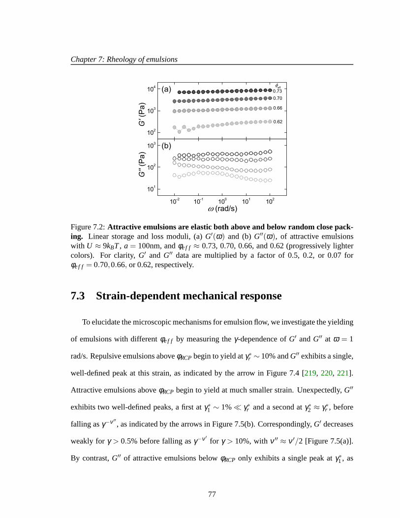
Chapter 7: Rheology of emulsions
102
103
104
10-2 10-1 100 101 102
101
102
103 (b)
0.73
0.62
0.66
0.70
G
' (P
a)
eff(a)
(rad/s)
G''
(Pa)
Figure 7.2:Attractive emulsions are elastic both above and below random close pack-ing. Linear storage and loss moduli, (a)G′(ω) and (b)G′′(ω), of attractive emulsionswith U ≈ 9kBT, a = 100nm, andφe f f ≈ 0.73, 0.70, 0.66, and 0.62 (progressively lightercolors). For clarity,G′ and G′′ data are multiplied by a factor of 0.5, 0.2, or 0.07 forφe f f = 0.70,0.66, or 0.62, respectively.
7.3 Strain-dependent mechanical response
To elucidate the microscopic mechanisms for emulsion flow, we investigate the yielding
of emulsions with differentφe f f by measuring theγ-dependence ofG′ andG′′ at ω = 1
rad/s. Repulsive emulsions aboveφRCPbegin to yield atγ∗r ∼ 10% andG′′ exhibits a single,
well-defined peak at this strain, as indicated by the arrow inFigure 7.4 [219, 220, 221].
Attractive emulsions aboveφRCP begin to yield at much smaller strain. Unexpectedly,G′′
exhibits two well-defined peaks, a first atγ∗1 ∼ 1%≪ γ∗r and a second atγ∗2 ≈ γ∗r , before
falling asγ−ν ′′, as indicated by the arrows in Figure 7.5(b). Correspondingly, G′ decreases
weakly for γ > 0.5% before falling asγ−ν ′for γ > 10%, withν ′′ ≈ ν ′/2 [Figure 7.5(a)].
By contrast,G′′ of attractive emulsions belowφRCP only exhibits a single peak atγ∗1 , as
77

Chapter 7: Rheology of emulsions
0.2 0.4 0.6 0.8 1.010-6
10-5
10-4
10-3
10-2
10-1
eff
G', G'' (
units
of
/a)
Figure 7.3:Elasticities of attractive and repulsive emulsions differbelow random closepacking but are similar above it. Linear storage and loss moduli,G′
p (solid points) andG′′
(open points), measured atω = 1 rad/s, normalized by the Laplace pressureσ/a, for bothattractive and repulsive emulsions of varyingφe f f. Attractive emulsions havea = 128nm,U ≈ 9kBT (circles),a = 106nm,U ≈ 7kBT (upward triangles), anda = 100nm,U ≈ 9kBT(squares); repulsive emulsions havea = 128nm (diamonds) anda = 106nm (downwardtriangles). The interfacial tensionσ = 6−9mN/m for the range of surfactant concentrationsused. Previous measurements ofG′
p (solid line) andG′′ (dashed line) for monodisperserepulsive emulsions [219], horizontally shifted to account for polydispersity, agree withour data. We findφRCP≈ 0.68−0.72, characteristic ofφRCP for spheres of comparablepolydispersity [237].
78
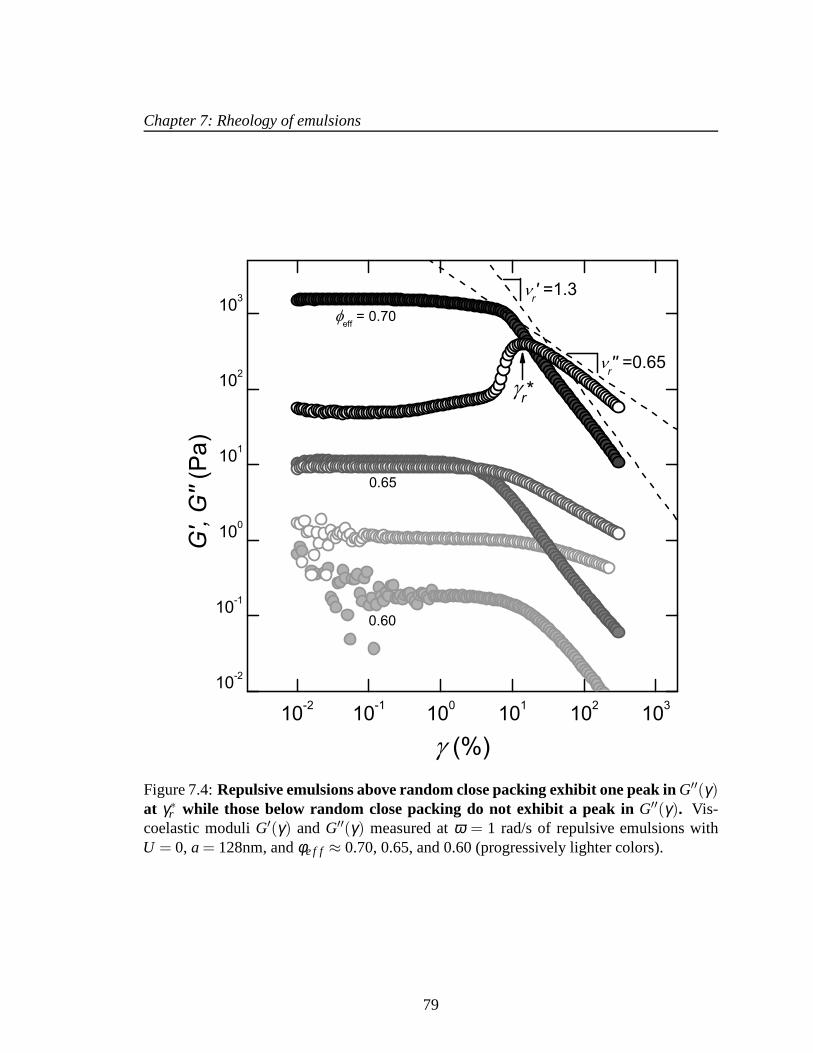
Chapter 7: Rheology of emulsions
10-2 10-1 100 101 102 103
10-2
10-1
100
101
102
103
(%)
0.60
r'' =0.65
r' =1.3
G',
G'' (
Pa)
r*
0.65
eff = 0.70
Figure 7.4:Repulsive emulsions above random close packing exhibit onepeak in G′′(γ)at γ∗r while those below random close packing do not exhibit a peak in G′′(γ). Vis-coelastic moduliG′(γ) andG′′(γ) measured atω = 1 rad/s of repulsive emulsions withU = 0, a = 128nm, andφe f f ≈ 0.70, 0.65, and 0.60 (progressively lighter colors).
79

Chapter 7: Rheology of emulsions
103
104
10-2 10-1 100 101 102 103
102
103
G' (
Pa)
0.62
G'' (
Pa)
(%)
eff = 0.66
1*
103
104
102
103
0.70
G' (
Pa)
*2
G'' (
Pa)
'' =0.85
' =1.75
eff = 0.73
1*
(d)
(c)
(b)
(a)
Figure 7.5: Attractive emulsions above random close packing exhibit two peaks inG′′(γ) at γ∗1 and γ∗2 while those below random close packing exhibit one peak atγ∗1 .Viscoelastic moduliG′(γ) andG′′(γ) measured atω = 1 rad/s of attractive emulsions withU ≈ 9kBT anda = 100nm (a-b) aboveφRCP (φe f f ≈ 0.73 and 0.70, progressively lightercolors) and (c-d) belowφRCP (φe f f ≈ 0.66 and 0.62, progressively lighter colors). Forclarity, G′ andG′′ data are multiplied by a factor of 0.7, 0.3, 0.8, or 0.2 for each φe f f goingfrom top to bottom. Straight lines indicateG′,G′′ ∼ γ−ν ′,−ν ′′
for largeγ.
80

Chapter 7: Rheology of emulsions
0.2 0.4 0.6 0.8 1.0
10-2
10-1
100
101
eff
* (%
)
Figure 7.6:Position of peaks inG′′(γ) for varying φe f f. Lower symbols representγ∗1 ,upper symbols represent eitherγ∗2 or γ∗r . Attractive emulsions havea = 128nm,U ≈ 9kBT(circles),a = 106nm,U ≈ 7kBT (upward triangles), anda = 100nm,U ≈ 9kBT (squares);repulsive emulsions havea = 128nm (diamonds) anda = 106nm (downward triangles).
shown in Figure 5(d), andG′ decreases smoothly forγ > 0.01−1% [Figure 7.5(c)].
To understand these results, we examine theφe f f-dependence ofγ∗1. Below φRCP, γ∗1
decreases with decreasingφe f f, as shown by the lower symbols in Figure 7.6; interestingly,
this is similar to behavior predicted for particulate colloidal gels connected by “weak links”
[238]. The elasticity of these emulsions results from the attractive interdroplet bonds; these
induce the formation of a stress-bearing connected networkcomprised of compact droplet
aggregates [224, 225, 226]. We expect the elasticity to be dominated by the weakest bonds
in the network, and hence yielding begins when these are broken. In this picture, a macro-
scopic deformation∆L deforms such a bond by∆L/(L/ζ ), whereL is the system size and
ζ is the characteristic distance between the weakest bonds. The force on such a bond is thus
ka∆L/(L/ζ ) = kaζ γ, whereka is the characteristic bond stiffness. Assuming that the bond
breaks at a fixed critical forceF∗ = kaζ γ∗1 , the critical strain amplitudeγ∗1 ∝ ζ−1. Our mea-
81

Chapter 7: Rheology of emulsions
surements ofγ∗1 thus imply thatζ increases with decreasingφe f f, suggesting that yielding
begins at fewer, sparser weak points asφe f f is decreased. This may reflect the changing
connectivity of the emulsion: the characteristic sizeξ of the droplet aggregates comprising
the emulsion also increases with decreasingφe f f [224, 226]. If the bonds between droplet
aggregates are the weakest in the emulsion [239, 240], we would expectζ ≈ ξ to increase
with decreasingφe f f, consistent with our results.
For increasingγ, attractive emulsions both below and aboveφRCP begin to yield and
exhibit a peak inG′′ at γ ∼ γ∗1 ; in contrast, those aboveφRCP exhibit an additional peak in
G′′ at γ ∼ γ∗2 [Figure 7.5]. This observation implies the existence of an additional process
by which the structure of these emulsions must relax before they can flow. This is likely due
to the compression of the droplets: aboveφRCP, attractive emulsions require larger strain
to fully yield through the irreversible rearrangements of densely-packed droplets, just as in
the repulsive case [220, 222]. This hypothesis is supported by our observation thatγ∗2 ≈ γ∗r .
The height of the first yielding peak inG′′(γ) decreases asφe f f increases aboveφRCP,
as shown in Figure 7.5(b), reflecting the increasing relative importance of these repulsive
interactions as the droplets are increasingly compressed [241].
To test the generality of these results, we perform similar measurements on an oil-
in-water emulsion stabilized by a different surfactant. The droplets are electrostatically
stabilized by SDS, an ionic surfactant that also forms freely-dispersed globular micelles,
and have low polydispersity (∼ 10%) [219, 236]. Similar to the case of P105-stabilized
emulsions,G′p measured for the SDS-stabilized emulsions has the same magnitude for
both attractive and repulsive emulsions packed aboveφRCP≈ 0.64 [Figure 7.7(a)]; this
indicates that the elasticity is dominated by the repulsiveforces deforming the droplets.
82

Chapter 7: Rheology of emulsions
0.4 0.5 0.6 0.7 0.8 0.9 1.0
100
101
eff
* (%
)
10-6
10-5
10-4
10-3
10-2
10-1
100G
p' (u
nits
of
/a)
(a)
(b)
Figure 7.7:Volume fraction-dependent behavior is similar for oil-in-water emulsionsstabilized by SDS.(a) Linear plateau storage modulus,G′
p [236], normalized by theLaplace pressureσ/a and (b) position of peaks inG′′(γ), for varying φe f f. Emulsionshavea = 250nm; attractive emulsions haveU ≈ 21kBT (circles) while repulsive emulsionshaveU < 1kBT (diamonds). The interfacial tensionσ = 9.8mN/m for the range of surfac-tant concentrations used. Upper symbols in (b) representγ∗2 while lower symbols representγ∗1 .
83

Chapter 7: Rheology of emulsions
For the repulsive emulsions,G′p drops precipitously asφe f f is decreased belowφRCP; by
contrast, the elasticity of the attractive emulsions persists far belowφRCP [Figure 7.7(a)].
Moreover,G′′(γ) of SDS-stabilized attractive emulsions aboveφRCP exhibits two peaks
at strainsγ∗1 ∼ 1%≪ γ∗r andγ∗2 ≈ γ∗r , as indicated in Figure 7.8(b). Correspondingly,G′
decreases weakly forγ > 0.5% before falling more quickly forγ > 10% [Figure 7.8(a)].
By contrast,G′′(γ) of the attractive emulsions belowφRCPexhibits a single peak at a strain
γ∗1 , andG′ decreases smoothly forγ > 1% [Figure 7.8]. These data are similar to those
obtained for P105-stabilized emulsions; this confirms thatour results are more general.
7.4 Time scales of the structural relaxation
The frequency-dependent mechanical response of emulsionsdirectly reflects the time
scales of their structural relaxation. For repulsive emulsions aboveφRCP, G′′(ω) exhibits a
shallow minimum atω ∼ 0.1−10 rad/s resulting from the combination of viscous loss at
high ω and the configurational rearrangements of the individual droplets at lowω [Figure
7.1] [219, 221]. In contrast, for attractive emulsions,G′′(ω) exhibits a minimum atωmin≥
10 rad/s, as shown in Figure 7.2. This further suggests that attractive interactions alter the
structural relaxation of emulsions.
The structural relaxation process through which attractive emulsions yield occurs at
frequencies much lower than is accessible in a linear rheological measurement, typical of
soft glassy materials [221]. We circumvent this problem by performingω-dependent mea-
surements holding the strain rate amplitudeγ = γω constant for different values ofγ. A
relaxation process of time scaleτ gives rise to a peak inG′′(ω) at a frequency proportional
to τ−1 [221]. We observe one peak inG′′(ω) for attractive emulsions withφe f f < φRCP;
84

Chapter 7: Rheology of emulsions
103
104
10-2 10-1 100 101 102 103102
103
104
0.59
0.62
0.65
(b)
G' (
Pa)
(a)
2*
1*
eff = 0.68
G''
(Pa)
(%)Figure 7.8:Strain-dependent behavior is similar for oil-in-water emulsions stabilizedby SDS.Viscoelastic moduli (a)G′(γ) and (b)G′′(γ) of attractive emulsions stabilized bySDS withU ≈ 21kBT anda = 250nm forφe f f ≈ 0.68, 0.65, 0.62, and 0.59 (progressivelylighter colors). Emulsions aboveφRCP(top two curves) show peaks inG′′ atγ∗1 andγ∗2 whilethose belowφRCP (lower two curves) show a single peak atγ∗1. For clarity,G′ andG′′ dataare multiplied by a factor of 0.7, 0.6, or 0.5 forφe f f = 0.65,0.62, or 0.59, respectively.
85

Chapter 7: Rheology of emulsions
10-3 10-2 10-1 100 101 102 103
101
102
103
104
10-2 10-1 100 101
10-1
100
101
102
.
.
. /b( )
.
.
G'/a
( ),
G''/a
( )
a( ),
b(
)
.
..
0.84
101
102
103
104
10-2 10-1 100 101
10-1
100
101
102
G'/a
( ),
G''/a
( )
.
.
0.95
.
.
.
a( ),
b(
)
(b)
(a)
Figure 7.9:Yielding of attractive emulsions is a shear-driven process. Constantγ fre-quency sweep measurements of viscoelastic moduliG′(ω) (solid points) andG′′(ω) (openpoints) for two samples witha = 100nm andU ≈ 9kBT aboveφRCP (a, φe f f ≈ 0.73) andbelowφRCP(b,φe f f ≈0.66), shifted onto a single master curve by normalizing by theshear-rate-dependent shift factorsa(γ) andb(γ). Inset: corresponding amplitude and frequencyshift factorsa(γ) (triangles) andb(γ) versusγ (squares).
86

Chapter 7: Rheology of emulsions
strikingly, we observe two peaks inG′′(ω) for those withφe f f > φRCP, as indicated in Fig-
ure 7.9, in stark contrast to the repulsive case [221]. This provides further confirmation that
attractive emulsions aboveφRCPundergo an additional relaxation process during yielding.
The data measured at differentγ can be scaled onto a master curve by rescaling the
moduli and frequency, as shown in Figure 7.9. The frequency scaling factorb(γ) ∼ τ−1
[221]. We explore its dependence onγ to directly probe how the time scales of the structural
relaxation processes of attractive emulsions depend on shear rate. We findb(γ)∼ τ−1 ∼ γν
with ν ≈ 0.8− 1 for both relaxation processes in attractive emulsions having φe f f both
below and aboveφRCP; two representative examples are shown in Figure 7.9 (inset). This
shear-driven behavior is similar to the yielding of colloidal gels [242] and to the yielding
of repulsive emulsions aboveφRCP [221].
Our data suggest a simple physical picture of emulsion flow. The rheology of emulsions
with slippery bonds of magnitudeU < 1kBT is similar to that of repulsive emulsions; in
stark contrast, emulsions withU > 7kBT show a dramatically enhanced elasticity below
φRCP. Moreover, their nonlinear rheology is markedly differentfrom the repulsive case.
These attractive emulsions begin to yield under sufficient shear through the breakage of
interdroplet bonds at weak points in the emulsion [227]. Attractive emulsions aboveφRCP
also undergo shear-induced configurational rearrangements of the densely-packed droplets,
similar to the repulsive case, at larger strain. This is reminiscent of the two-step yielding of
attractive colloidal glasses [243]. How this behavior changes with intermediate values of
U remains to be explored.
Emulsions are often used to model many other diverse physical systems and are crucial
in various technological processes. We find that their linear and nonlinear rheology depend
87

Chapter 7: Rheology of emulsions
sensitively on the interactions between the droplets. Our results may thus be a useful input
to such models and could help guide processes designed to control emulsion elasticity and
flow behavior.
88
Chapter 8
Buckling and crumpling of
nanoparticle-coated droplets
Suspensions of fluid droplets coated with solid colloidal particles are commonly known
as “Pickering” emulsions. Particles with suitable surfacechemistries can adsorb at the
droplet surfaces strongly, with an energy of up to hundreds of kBT. As a result, Pickering
emulsion droplets can be exceptionally stable against coalescence and Ostwald ripening,
making them useful for a wide variety of applications in which their interfacial properties
play a key role. For example, Pickering emulsion droplets are promising candidates for
encapsulating, delivering, or controllably releasing poorly soluble drugs [244]. They have
also been used as templates for fabricating hierarchical porous materials for catalysts or
filters [245].
The stability of Pickering emulsion droplets is due to the dense packing of a strongly
bound layer of colloidal particles at the fluid-fluid interface [246, 247]; this layer is hy-
pothesized to behave as a two-dimensional solid [248, 249, 250, 251, 252]. However,
89

Chapter 8: Buckling and crumpling of nanoparticle-coated droplets
experimental approaches to verifying this suggestion havebeen limited toflat fluid inter-
faces [249, 253, 254, 255, 256]. The solid-like nature of particle-coated surfaces is also
often used to describe the curved interfaces of fluid droplets; for example, this assumption
is essential to the interpretation of rheological measurements of densely packed Pickering
emulsions [251]. Nevertheless, direct experimental evidence of the solid-like nature of the
surface of particle-coated droplets remains lacking.
An unambiguous way to confirm the solid-like behavior of a thin shell is to observe
buckling when it is strongly deformed. For example, as the volume of a thin elastic shell is
reduced, compressive stresses build up on its surface, causing localized mechanical insta-
bilities such as sharp points and bends to develop [257]. The proliferation of these localized
instabilities results in a shell with a crumpled morphology. The crumpling of fluid-filled
shells has been achieved experimentally either by uncontrollably dissolving or by evap-
orating the interior fluid for several porous capsules [258, 259, 260, 261], or by using an
externally imposed osmotic pressure [262, 263]. Few such studies exist for Pickering emul-
sions [264]. A method to controllably induce compressive stresses at Pickering emulsion
droplet surfaces is thus highly desirable to directly test their mechanical properties.
In this Chapter7, we study the structural transitions of large numbers of nanoparticle-
coated droplets as fluid is controllably pumped out of the droplet interiors. We find that a
significant fraction of droplets buckle or crumple upon volume reduction, confirming the
hypothesis that their interfaces behave like solids. The number of non-spherical droplets
as well as the resultant droplet morphology is highly dependent on the amount of volume
reduction and the average size of the droplets. All of the morphologies we observe are sta-
7Based on “Controlled buckling and crumpling of nanoparticle-coated droplets”,S. S. Datta, H. C. Shum,and D. A. Weitz,Langmuir, 26, 18612 (2010).
90

Chapter 8: Buckling and crumpling of nanoparticle-coated droplets
ble over a period of at least several hours. Many of these are strikingly similar to structures
observed or predicted for buckled thin continuum elastic shells. The technique presented
here provides a new and straightforward way to study the deformation behavior of thin
fluid-filled granular shells.
8.1 Formulation of Pickering emulsions
Ethylene glycol (anhydrous, 99.8%, Sigma-Aldrich), chlorobenzene (CHROMASOLV,
for HPLC, 99.9%, Sigma-Aldrich), glycerol (ACS reagent, 99.5%, Sigma-Aldrich), and
hydrophobic silica nanoparticles (diameter≈ 15 nm±30%, Tol-ST, Nissan Chemical Inc.)
were used as received. Some samples were made using ethyleneglycol and chloroben-
zene dried by tumbling with molecular sieves (3A, beads, 4-8 mesh, Sigma-Aldrich) and
filtered with a 0.2µm filter. The samples prepared with the dried reagents showedno no-
ticeable difference in the final results, as compared to samples prepared with reagents used
as received.
Emulsions were produced at a volume fraction of∼61% by mixing known masses of
ethylene glycol containing 1% glycerol (to minimize Ostwald ripening) and chlorobenzene
containing a suitable amount of nanoparticle suspension. These were mechanically agitated
by intensive vortexing for 10-40 minutes. This procedure forms extremely stable “water-
in-oil” emulsions with ethylene glycol/glycerol as the dispersed phase and chlorobenzene
as the continuous phase. This suggests that the silica nanoparticles have a contact angle
close to 90◦, but are more preferentially wet by chlorobenzene [265]. Furthermore, these
samples have surprisingly low polydispersities (∼30%) given the inhomogeneous shear
rates that arise during emulsification.
91
Chapter 8: Buckling and crumpling of nanoparticle-coated droplets
Ethylene glycol is partially soluble in chlorobenzene at a concentration of∼1.5µL g−1.
This is determined in two ways. First, the conductivities ofboth unsaturated chlorobenzene
(σunsat) and chlorobenzene that has been saturated with ethylene glycol (σsat) were mea-
sured, as well as the conductivity of ethylene glycol (σEG). The saturation concentration
of ethylene glycol in chlorobenzene (csat) was then calculated by linearly interpolating be-
tweenσunsat andσEG using the relationσsat ≈ σunsat+ csatσEG. Second, the saturation
concentration was directly measured by mixing measured amounts of ethylene glycol with
chlorobenzene until the resulting solution is no longer visibly homogenous. Values of sat-
uration concentration of ethylene glycol in chlorobenzenefrom the two measurements are
in good agreement.
To controllably pump a known volume of fluid from inside the droplets, a measured
quantity of emulsion is added to a suitable amount of unsaturated chlorobenzene. This is
then tumbled gently for several days.
Droplet morphologies were characterized using optical microscopy at a range of mag-
nifications (10x-100x), using either a Leica SP5 confocal microscope operating in bright-
field mode or a Nikon Eclipse TE2000-E. Samples were imaged insealed glass capillaries
or sealed imaging chambers made from polyether ether ketone(PEEK) spacers.
8.2 Volume-controlled morphological transitions
We use hydrophilic silica nanoparticles that are coated with a diffuse layer of alkane,
rendering them partially hydrophobic and partially hydrophilic. Thus, they are wetted by
both dispersed and continuous phases, and the three-phase contact angle characterizing the
placement of the nanoparticles at the interface between thetwo phases is close to 90◦. As a
92

Chapter 8: Buckling and crumpling of nanoparticle-coated droplets
result, once a nanoparticle is mechanically driven to this interface during the emulsification
process, it is confined within a potential well of depth as large as hundreds ofkBT [266].
This makes the emulsions used in this work highly stable for at least several weeks.
Due to the strong attachment of the nanoparticles to the droplet surfaces, the average
droplet size is controlled by the concentration of nanoparticles used to prepare the samples
[267]. The average droplet diameterd is related to the volume concentrationcp of nanopar-
ticles with respect to the dispersed phase byd = 8φAnap/cp, whereφA is the fraction of
the droplet surfaces that is covered with nanoparticles,n is the average number of nanopar-
ticle layers covering the droplets, andap is the nanoparticle radius. This equation fits our
data very well over a wide range, as shown in Figure 8.1. Usingthis fit, we estimate that
the droplet surfaces are coated with a monolayer of nanoparticles with surface coverage
φA = 80±2%.
A closed solid shell with a fixed surface area must deform as its volume is reduced
and compressive stresses develop in the shell wall. These stresses are typically relieved
through buckling events, in which the shell is strongly deformed only at points and lines
on its surface [257]. Motivated by this, we develop a technique to study the mechanical
properties of our Pickering emulsion droplet surfaces by reducing their average volume in a
controlled manner. To achieve volume reduction, we use a dispersed phase whose solubility
in the continuous phase is measured to be∼ 0.17 vol%. Thus mixing a Pickering emulsion
with unsaturated continuous phase causes a finite amount of the dispersed phase to be
pumped out of the droplets until the solubility limit of the continuous phase is reached. We
calculate the average decrease in droplet volume∆V relative to the original droplet volume
V0 to be ∆V/V0 ≈ 0.0017Vadd/φVs, whereφ is the emulsion volume fraction,Vs is the
93

Chapter 8: Buckling and crumpling of nanoparticle-coated droplets
Figure 8.1: Average droplet diameter d of Pickering emulsion prepared at differ-ent nanoparticle concentrationscp. White square represents a sample made by addingnanoparticles to the sample represented by the white circle; white triangle represents a sam-ple made by adding more dispersed phase to the sample represented by the white square.Vertical error bars indicate standard deviation of area-weighted size distribution, while hor-izontal error bars indicate estimated uncertainty incp. Solid line indicates inverse depen-dence ofd with cp (d = 8φAnap/cp) as discussed in the text.
94

Chapter 8: Buckling and crumpling of nanoparticle-coated droplets
Figure 8.2:Forcing droplets to buckle by shrinking them. (A) Schematic illustrating thecontrolled reduction of droplet volume of Pickering emulsion droplets. (B) Optical micro-graph of a crumpled droplet with fluorescently labeled dispersed phase (green overlaid);scale bar is 5µm.
initial sample volume, andVadd is the volume of additional unsaturated continuous phase.
For each value ofVadd, we use optical microscopy to quantify the fraction of droplets that
were clearly buckled or crumpled, analyzing a total of 3759 droplets. The pumping process
presented here is analogous to applying a pressure difference across the particle-coated
droplet surface. Similar to studies of osmotically-induced buckling of hollow capsules
[262], our technique involves the addition of a chemical speciesthat forces solvent to be
expelled from the droplet interiors. A key advantage of thisapproach is that it enables the
simultaneous investigation of the buckling of large numbers of Pickering emulsion droplets
of varying sizes, yielding statistics of this process unlike approaches using pendant drop
tensiometry [268] or a syringe [264] to shrink individual macroscopic droplets.
To study the mechanical nature of the particle-coated droplet surfaces, we observe their
morphologies as their volume is reduced. Strikingly, a considerable fraction of the droplets
95

Chapter 8: Buckling and crumpling of nanoparticle-coated droplets
become non-spherical due to buckling or crumpling (Figure 8.2), unambiguously demon-
strating that their surfaces are solid. AsVadd and hence the degree of pumping is increased,
more droplets are deformed. To further understand the properties of the droplet surfaces,
we explicitly consider the microscopic interactions between the nanoparticles.
The van der Waals interaction can be estimated byUvdW = Aap/12l , whereA is
the Hamaker constant,ap is the nanoparticle radius, andl is the distance between the
nanoparticle surfaces. Using typical values ofA ≈ 10− 20 J andl ≈ 0.5 nm, we esti-
mateUvdW ≈ 3kBT and hence, the two-dimensional shear modulusG′2D ≈UvdW/a2
p ≈ 0.2
mN m−1.
In the bulk continuous phase, the nanoparticles possess very weak attractions, whereas
in the bulk dispersed phase the nanoparticles are much more strongly attractive due to the
interpenetration of the alkyl chains coating the colloidalparticles. The maximum value
of these attractive interactions can be estimated byUattr ≈ πapL2|1/2− χ|/vm whereL
is the thickness of the surface coating layer,χ is the Flory-Huggins interaction parameter
appropriate for the dispersed phase, andvm is the volume of a solvent molecule [269].
Using suitable values ofL ≈ 0.5 nm, χ ≤ 10, andvm ≈ 3 A3, we estimate a maximum
value ofUatt ≈ 104kBT; thus,G′2D ≈Uatt/a2
p ≈ 700 mN m−1.
By modeling a particle monolayer at a fluid interface interacting via capillary forces
[270] as an isotropic solid, Vellaet al. [249] and Arditty et al. [251]independently devel-
oped an estimate for its Youngs modulus:E ∼ 5γ/ap, whereγ is the fluid-fluid interfacial
tension andap is the particle radius. Using the interfacial tension for our system mea-
sured using pendant drop tensiometry (γ ≈ 7 mN m−1), we use the expression forE to
estimate the energy of capillary interactions asUcap≈ Ea3p = 5γa2
p ≈ 500kBT and hence
96

Chapter 8: Buckling and crumpling of nanoparticle-coated droplets
Figure 8.3: Rheology of the particle interface. Interfacial shear and loss moduliG′2D
(closed circles) andG′′2D (open circles) as a function of applied strain at a fixed angular
frequency of 5 rads s−1 (left image) and as a function of angular frequency at a fixed strainof 0.1% (right image).
the two-dimensional shear modulusG′2D ≈Ucap/a2
p ≈ 40 mN m−1.
These simple estimates suggest that the surface shear modulus at the droplet interfaces
is likely to be determined predominantly by interparticle attractions due to their surface
functionalization and capillary interactions, and is in the rangeG′2D ≈ 40−700 mN m−1.
We also use interfacial rheology to directly measureG′2D for the flat fluid-fluid interface
saturated with an excess of nanoparticles. We place an excess amount of nanoparticles at
a flat interface between ethylene glycol and chlorobenzene and use an Anton-Paar Phys-
ica MCR501 rheometer equipped with an Interfacial RheologySystem. We use a bicone
geometry to directly measure the interfacial elastic and loss moduliG′2D andG′′
2D as a func-
tion of applied strain and frequency. The results, shown in Figure 8.3, indicate that the
layer of nanoparticles has mechanical properties similar to a soft glassy material [256] with
G′2D ≈ 0.05 Pa m = 50 mN m−1.
Furthermore, because our nanoparticles are highly polydisperse, their structure at a
97

Chapter 8: Buckling and crumpling of nanoparticle-coated droplets
droplet surface is likely to be amorphous, in contrast to systems with monodisperse par-
ticles in which crystalline defects play a significant role [271, 272]. Thus, the droplet
surfaces can be thought of as thin, porous, solid granular shells. The approach presented
here is a powerful means to study volume-controlled morphological transitions of fluid-
filled granular shells in a well-defined manner, by subjecting large numbers of droplets to
the same degree of pumping.
8.3 Size-dependent morphologies
Unlike the case of a sheet, deforming a thin elastic shell requires it to both bend and
stretch [273]; thus, the buckling and crumpling behavior of such shells is typically un-
derstood by considering the energies associated with both of these deformation modes.
Because stretching deformations require more energy than bending [274], they tend to be
focused at points and lines, leading to localized mechanical instabilities that develop as the
shell is increasingly deformed. While the mechanical properties of densely packed par-
ticles at fluid-fluid interfaces is typically interpreted within the framework of continuum
elasticity [248, 249], it is still not clear that this approach is appropriate forparticle-coated
droplets [275, 276]. To explore the similarities between classical thin elastic shells and our
particle-coated droplets, we study the size dependence of droplet buckling as well as the
morphologies of buckled and crumpled droplets.
By considering the shell size dependence of the energy required to form a depression in
an elastic spherical shell, an analysis based on classical elasticity theory predicts that larger
droplets should buckle more easily than smaller droplets [258]. To test this, we prepare
samples consisting of droplets of three different average sizes, and controllably reduce
98

Chapter 8: Buckling and crumpling of nanoparticle-coated droplets
Figure 8.4:Volume change controls amount of buckling.A plot of the fraction of buck-led/crumpled droplets as a function of calculated relativechange in droplet volume forsamples of average droplet diametersd = 14.7µm (red circles), 34.7µm (blue squares),and 44.1µm (green triangles). Solid lines are guides to the eye. Insetshows optical micro-graphs of two different samples: left has undergone weak pumping, right has undergonestronger pumping.
99

Chapter 8: Buckling and crumpling of nanoparticle-coated droplets
their average volume. Crucially, our data clearly show thatlarger droplets require a smaller
relative decrease in their volume than do smaller droplets to crumple by the same fraction,
as shown in Figure 8.4. This suggests that larger droplets crumple more easily, which is in
agreement with the idea of having a thin shell of densely-packed colloids covering the fluid
droplets.
Our approach is a useful way to characterize the morphological transitions undergone
by droplets at varying degrees of pumping. For weak pumping,the droplets are often non-
spherical, forming polyhedra with multiple flat facets separated by straight edges (Figure
8.5A). Similar shapes have been achieved previously for particle-coated bubbles or droplets
that have coalesced or that have forcibly undergone plasticdeformation [277]. In our sys-
tem, however, it is likely that such shapes arise from the presence of localized defects in
the granular shell. These can mediate the structural transitions of the shell due to volume
pumping in a manner similar to that in which fivefold disclinations can lead to faceting
of crystalline granular shells [278]. For intermediate pumping, droplets develop dimples
or corrugations of size∼ 1− 10µm on their surfaces (Figure 8.5B). These are reminis-
cent of post-buckling structures for thin shells under pressure [279] or core-shell structures
whose shells have experienced significant compressive stresses [262, 259]. As pumping
increases, droplets have more crumpled morphologies with increasing numbers of dim-
ples developing; this is consistent with the notion that crumpling may be thought of as a
sequential buckling process [257]. For stronger pumping, dimples grow into cusps and
ridges spanning a wide range of size scales (∼ 0.1− 100µm) joining points of maximal
curvature (Figure 8.5C). Due to the fixed surface area of the shell, these cusps and ridges
start to interact with each other as fluid is pumped out of the droplets, as demonstrated
100

Chapter 8: Buckling and crumpling of nanoparticle-coated droplets
by the increasing numbers of longer and sharper cusps and ridges shown in Figure 8.5C.
This suggests that in-plane stretching of the nanoparticlenetwork at the droplet surface is
energetically more costly than bending, as in the case of thin continuum sheets, and stress
is localized heterogeneously on the droplet surface.
These observations strongly support the hypothesis that a sufficiently densely packed
layer of colloidal particles at a fluid-fluid interface acts like a solid. In particular, the
nonuniform capillary stresses associated with the highly deformed morphologies adopted
by our droplets must be supported by localized stresses in the solid granular shell; other-
wise, these would be pulled back to a spherical shape by the fluid-fluid interfacial tension
[277, 250, 280, 281]. Moreover, all observed morphologies are “frozen-in”; they are stable
over an observation time of hours. Furthermore, when subjected to a shear flow, buckled
droplets undergo rigid-body rotation as expected for a solid shell. This is clearly different
from the tank treading motion expected for a droplet with a fluid surface [282], confirming
that the particles form a solid layer at the droplet interfaces.
In addition to the typical morphologies shown in Figure 8.5A-C, droplets exhibit a num-
ber of other buckled structures. These include multifaceted polyhedral indentations con-
sisting of up to eight vertices (Figures 8.5D and 8.6); sharply-defined creases and ridges
that meet at individual points (Figure 8.5E); and elongatedshapes strongly reminiscent of
folded monosulcate lily pollen grains [285] (Figure 8.5F). The observation of such a variety
of buckled structures suggests that the mechanical properties of the interfaces of the Pick-
ering droplets are non-uniform. The morphologies observedare strikingly similar to those
seen for thin continuum elastic shells possessing locally more compliant areas on their sur-
face. For example, a spherical cap with a single point-like “weak spot” develops a faceted
101

Chapter 8: Buckling and crumpling of nanoparticle-coated droplets
Figure 8.5:Optical micrographs of different buckled droplets. (A-C) show characteris-tic shapes at increasing levels of pumping, ranging from weak pumping (A), intermediatepumping (B), and strong pumping (C). Typical buckled structures also include multifacetedpolyhedral indentations (D), stretching ridges,d-cones, and “swallowtail” folds (E), andelongated “football” structures (F). Bottom-left inset to(F) shows representative end-onview. All scale bars are 5µm. Colored insets show macroscopic analogues of buckledstructures: point indentation of a bottle using a pen [283] (D), creases and ridges in crum-pled paper [284] (E), and elongated dessicated pollen granule [285] (F).
Figure 8.6:Optical micrographs of different buckled droplets. We observe multifacetedpolyhedral indentations having three (A), four (B), and six(C) vertices. All scale bars are5 µm.
102

Chapter 8: Buckling and crumpling of nanoparticle-coated droplets
polyhedral indentation within its surface upon volume reduction, similar to the structure
shown in Figure 8.5D [283, 285]. In folded sheets and large crumpled shells, multiple
point-like singularities connected by stretching ridges give rise to morphologies similar to
that shown in Figure 8.5E [257, 286, 287, 284]. A “weak spot” extended along a line on
the surface of a shell, such as at a grain boundary [271], gives rise to an elongated structure
upon volume reduction as in the droplet shown in Figure 8.5F [285]. These comparisons
suggest that the observed non-uniform crumpling morphologies can be attributed to hetero-
geneities in the colloidal shell of the Pickering droplets that inevitably arise during sample
preparation. The compliant areas in the surfaces of Pickering emulsions likely guide the
development of deformations during volume reduction, giving rise to the rich diversity of
post-buckling morphologies. Thus, by tuning the arrangements of particles at the droplet
interfaces, the crumpling morphologies can potentially becontrolled.
In conclusion, we present a straightforward and general method for buckling and crum-
pling statistically significant numbers of nanoparticle-coated droplets by pumping fluid out
of the droplet interiors. Increasing numbers of droplets buckle and crumple as their aver-
age volume is reduced. The extent to which droplets are buckled or crumpled depends on
the average droplet size, with larger droplets crumpling more easily than smaller droplets in
agreement with ideas based on continuum elasticity theory.As they undergo volume reduc-
tion, droplets become increasingly non-spherical and develop progressively more dimples,
suggesting that crumpling may be thought of as a sequential buckling process. For stronger
pumping, cusps and sharply curved ridges develop and grow. The structures of our buckled
Pickering emulsions are strikingly similar to the buckled shapes of thin continuum elastic
shells. Our approach is a new means to realize stable non-spherical fluid droplets, and our
103
Chapter 8: Buckling and crumpling of nanoparticle-coated droplets
observations show that the droplet surfaces are solid-like. The technique presented here
offers a route to systematically study the morphological transitions of thin fluid-filled gran-
ular shells undergoing volume reduction and to explore the similarities between these and
“classical” thin elastic shells.
104

Chapter 9
Buckling of inhomogeneous
microcapsules
An important stimulus for microcapsule release is an externally imposed stress. This
idea is central to one of the earliest and most ubiquitous applications of microcapsules: to
encapsulate and release the colorless ink used in carbonless copy paper. The microcapsules
coat each sheet of paper, only releasing the encapsulated ink when pressed on sufficiently
hard by a pen; the released ink then reacts with a developer coating the underlying sheet,
forming a mark that reproduces the pen’s trace [81]. In this application, as in numerous
others, the utility of the microcapsules depends sensitively on the mechanical properties of
their shells.
One common way of characterizing this behavior is to monitorhow a microcapsule re-
sponds to an externally-imposed pressure. For small pressures, a homogeneous, spherical
shell, characterized by a uniform thickness, supports a compressive stress, and it shrinks
isotropically. Above a threshold pressure, however, this shrinkage becomes energetically
105

Chapter 9: Buckling of inhomogeneous microcapsules
prohibitive; instead, the shell buckles, reducing its volume by forming a localized in-
dentation at a random position on its surface. For the case ofa homogeneous shell, this
threshold pressure can be calculated using a linearized analysis of shell theory [279, 288],
while the exact morphology of the shell after it buckles requires a full nonlinear analysis
[289, 290, 283]. However, many microcapsule shells are inhomogeneous, characterized by
spatially-varying thicknesses and elastic constants. Such inhomogeneities can strongly in-
fluence how a shell buckles [285, 279, 291, 292, 293, 294, 295]. Unfortunately, despite its
common occurrence in real microcapsules, exactly how inhomogeneity influences the onset
of buckling, as well as the microcapsule morphology after buckling, remains to be eluci-
dated. A deeper understanding requires careful investigations of the buckling of spherical
microcapsules with shells having tunable, well-defined, inhomogeneities.
In this Chapter8, we use a combination of experiments, theory, and simulation to study
the buckling of spherical microcapsules with inhomogeneous shells of non-uniform thick-
nesses. We show that the onset of buckling, above a thresholdexternal osmotic pressure,
is well described by shell theory; however, even above this threshold, the microcapsules do
not buckle immediately. We find that the time delay before theonset of buckling decreases
as the shells are made more inhomogeneous; these dynamics can be quantitatively under-
stood by coupling shell theory with Darcy’s law for flow through a porous microcapsule
shell, even for highly inhomogeneous shells. Moreover, we find that the shell inhomogene-
ity guides the folding pathway taken by a microcapsule during and after buckling. We use
8Based on “Delayed buckling and guided folding of inhomogeneous capsules”,S. S. Datta∗, S-H Kim∗,J. Paulose∗, A. Abbaspourrad, D. R. Nelson, and D. A. Weitz,Physical Review Letters109, 134302 (2012)and “Controlling release from double emulsion-templated microcapsules”,S. S. Datta∗, A. Abbaspourrad∗,E. Amstad, J. Fan, S-H Kim, M. Romanowsky, H. C. Shum, B. J. Sun, A. S. Utada, M. Windbergs, S. Zhu,and D. A. Weitz, to be submitted (2013) *Equal contribution.
106

Chapter 9: Buckling of inhomogeneous microcapsules
these insights to controllably create novel colloidal structures using buckling.
9.1 Microcapsule fabrication
Microcapsules can be fabricated using a variety of techniques, including spray drying
[296, 297, 298], electrospraying [299, 300, 301], coextrusion [302, 303, 304], interfacial
polymerization [305, 306, 307], polymer phase separation [308, 309], layer-by-layer depo-
sition [74, 310, 311], or membrane emulsification [312, 313]. However, the highly variable
shear typically used in these approaches yields microcapsules with polydisperse sizes and
structures, and consequently, poorly controlled loading levels and release kinetics – even
within the same batch. This can severely limit the use of microcapsules in many practical
applications. Microfluidic technologies offer exquisite control over the flows of multiple
fluids, and thus, a way to overcome these limitations. One particularly promising route
is the use of microfluidics to produce double emulsions, drops of the core material within
drops of another fluid, which are themselves suspended in a continuous fluid phase. The
middle phase can then be solidified, yielding microcapsules. The interfacial tensions be-
tween the different fluids forces the drops to be spherical; moreover, the drop sizes are
determined by the shear forces exerted on the flowing fluids, which can be carefully tuned
in a microfluidic device. As a result, double emulsion drops generated in microfluidics, and
the microcapsules made from them, can be highly monodisperse, with compositions and
morphologies that can be manipulated with a remarkable degree of accuracy.
We fabricate monodisperse thin-shelled microcapsules using water-in-oil-in-water (W/O/W)
droplets prepared with two different types of glass capillary microfluidic devices. To
make microcapsules withh0/R0 = 0.017, we use a device composed of a hydrophobic
107
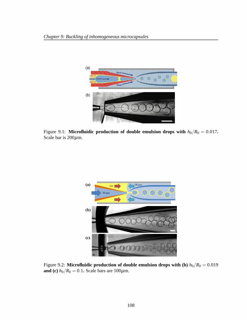
Chapter 9: Buckling of inhomogeneous microcapsules
Figure 9.1: Microfluidic production of double emulsion drops with h0/R0 = 0.017.Scale bar is 200µm.
Figure 9.2:Microfluidic production of double emulsion drops with (b) h0/R0 = 0.019and (c)h0/R0 = 0.1. Scale bars are 100µm.
108

Chapter 9: Buckling of inhomogeneous microcapsules
Figure 9.3:Monodisperse microcapsules.Scale bars in (a) and (b) are 500µm and 200µm, respectively.
Figure 9.4: SEM showing inhomogeneous microcapsule shell.Shells buckle at thethinnest part; as a result, the thinnest part contacts the thickest part of the shell. Rightpanel: the left arrow shows the thickest part of the shell, and the right arrow shows thethinnest part of the shell; the solid in between the two partsof the shell is precipitated PVA.Scale bar is 2µm.
109
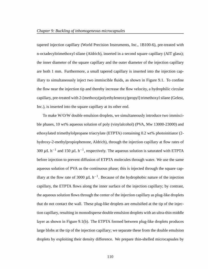
Chapter 9: Buckling of inhomogeneous microcapsules
tapered injection capillary (World Precision Instruments, Inc., 1B100-6), pre-treated with
n-octadecyltrimethoxyl silane (Aldrich), inserted in a second square capillary (AIT glass);
the inner diameter of the square capillary and the outer diameter of the injection capillary
are both 1 mm. Furthermore, a small tapered capillary is inserted into the injection cap-
illary to simultaneously inject two immiscible fluids, as shown in Figure 9.1. To confine
the flow near the injection tip and thereby increase the flow velocity, a hydrophilic circular
capillary, pre-treated with 2-[methoxy(polyethyleneoxy)propyl] trimethoxyl silane (Gelest,
Inc.), is inserted into the square capillary at its other end.
To make W/O/W double emulsion droplets, we simultaneously introduce two immisci-
ble phases, 10 wt% aqueous solution of poly (vinylalcohol) (PVA, Mw 13000-23000) and
ethoxylated trimethylolpropane triacrylate (ETPTA) containing 0.2 wt% photoinitiator (2-
hydroxy-2-methylpropiophenone, Aldrich), through the injection capillary at flow rates of
300µL h−1 and 150µL h−1, respectively. The aqueous solution is saturated with ETPTA
before injection to prevent diffusion of ETPTA molecules through water. We use the same
aqueous solution of PVA as the continuous phase; this is injected through the square cap-
illary at the flow rate of 3000µL h−1. Because of the hydrophobic nature of the injection
capillary, the ETPTA flows along the inner surface of the injection capillary; by contrast,
the aqueous solution flows through the center of the injection capillary as plug-like droplets
that do not contact the wall. These plug-like droplets are emulsified at the tip of the injec-
tion capillary, resulting in monodisperse double emulsiondroplets with an ultra-thin middle
layer as shown in Figure 9.1(b). The ETPTA formed between plug-like droplets produces
large blobs at the tip of the injection capillary; we separate these from the double emulsion
droplets by exploiting their density difference. We prepare thin-shelled microcapsules by
110

Chapter 9: Buckling of inhomogeneous microcapsules
photo-polymerization of the droplet middle phase, ETPTA.
To make microcapsules withh0/R0 = 0.019 and 0.1, we use a device composed of hy-
drophobic injection and collection capillaries as shown inFigure 9.2(a). The innermost
aqueous phase is injected through the injection capillary and the middle ETPTA phase is
injected through the interstices of the injection and the square capillaries. The continuous
aqueous phase is injected through the interstices of the collection and the square capillar-
ies as a counter flow to the innermost and the middle phases. These three streams flow
coaxially through the orifice of the collection capillary, making double emulsion drops in
a dripping mode. Forh0/R0 = 0.019, flow rates of the innermost, the middle, and the con-
tinuous phases are kept at 400, 80, 2000µL h−1, respectively, as shown in Figure 9.2(b).
For h0/R0 = 0.1, flow rates of the innermost, the middle, and the continuousphases are
kept at 200, 100, 2000µL h−1, respectively, as shown in Figure 9.2(c). Optical microscope
images of monodisperse microcapsules withtw = 1 min are shown in Figure 9.3.
To make microcapsules with two or three spherical compartments, we employ two-step
emulsification in a capillary microfluidic device. Inner water drops are produced at the tip
of small tapered capillary in a dripping mode, which in turn are encapsulated into oil drops
at the tip of injection capillary. Through precise control of flow rates of three streams, we
can manipulate generation frequency of inner water drops and outer oil drops. Therefore,
the number of inner drops confined in outer drop is controllable. To make the thin shell,
the flow rate of middle oil stream is maintained to be small enough to encapsulate two or
three inner drops with nonspherical envelope. The nonspherical double emulsion drops are
polymerized byin-situ UV irradiation, resulting in microcapsules with multiple spherical
compartments.
111

Chapter 9: Buckling of inhomogeneous microcapsules
The PVA solution is less dense than the oil; as a result, afterthe droplets are produced
and collected, the light inner water droplets gradually rise within them. This causes the oil
to gradually thin on the top side of each droplet and thicken on the bottom [314]. We exploit
this effect to prepare microcapsules, with outer radiusR0, and spatially-varying shell thick-
nessh(θ) ≈ h0−δcosθ ; θ is measured from the top of the gravitationally-oriented shell,
h0 is the average shell thickness, andδ is the total distance moved by the inner droplet, as
shown schematically in Figure 9.5(a). The shell inhomogeneity can thus be quantified by
the ratioδ/h0. We use UV light to polymerize the oil either as the microcapsules are pro-
ducedin situ, or after different average waiting times,tw; this enables us to prepare separate
batches of microcapsules characterized by varying degreesof shell inhomogeneity. We use
either scanning electron microscopy (SEM) or confocal microscopy to directly measure the
microcapsule geometrical characteristics.
Microcapsules photopolymerizedin situare prepared in the following manner: As soon
as the drops flow out from the nozzle of a microfluidic device towater bath containing 8
wt% aqueous solution of PVA which is saturated with ETPTA, they are polymerized by
continuous UV irradiation (Omnicure S1000).
Microcapsules withtw = 5 s or 1 min are prepared in the following manner: As they are
continuously produced from the nozzle of the microfluidic device, the droplets are collected
into a chamber containing 8 wt% aqueous solution of PVA saturated with ETPTA and are
repetitively irradiated with UV irradiation (Omnicure S1000) of duration 1 second, fully
polymerizing the ETPTA into a thin solid shell, every 2× tw. This forms a population
of microcapsules that have remained quiescent in the collection chamber for an average
waiting time oftw before polymerization.
112
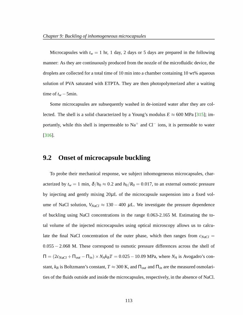
Chapter 9: Buckling of inhomogeneous microcapsules
Microcapsules withtw = 1 hr, 1 day, 2 days or 5 days are prepared in the following
manner: As they are continuously produced from the nozzle ofthe microfluidic device, the
droplets are collected for a total time of 10 min into a chamber containing 10 wt% aqueous
solution of PVA saturated with ETPTA. They are then photopolymerized after a waiting
time of tw−5min.
Some microcapsules are subsequently washed in de-ionized water after they are col-
lected. The shell is a solid characterized by a Young’s modulusE ≈ 600 MPa [315]; im-
portantly, while this shell is impermeable to Na+ and Cl− ions, it is permeable to water
[316].
9.2 Onset of microcapsule buckling
To probe their mechanical response, we subject inhomogeneous microcapsules, char-
acterized bytw = 1 min, δ/h0 ≈ 0.2 andh0/R0 = 0.017, to an external osmotic pressure
by injecting and gently mixing 20µL of the microcapsule suspension into a fixed vol-
ume of NaCl solution,VNaCl ≈ 130− 400 µL. We investigate the pressure dependence
of buckling using NaCl concentrations in the range 0.063-2.165 M. Estimating the to-
tal volume of the injected microcapsules using optical microscopy allows us to calcu-
late the final NaCl concentration of the outer phase, which then ranges fromcNaCl =
0.055− 2.068 M. These correspond to osmotic pressure differences across the shell of
Π = (2cNaCl + Πout−Πin)×NAkBT = 0.025−10.09 MPa, whereNA is Avogadro’s con-
stant,kB is Boltzmann’s constant,T ≈ 300 K, andΠout andΠin are the measured osmolari-
ties of the fluids outside and inside the microcapsules, respectively, in the absence of NaCl.
113

Chapter 9: Buckling of inhomogeneous microcapsules
For each batch of microcapsules studied, we monitor an average of 75 microcapsules over
time using optical microscopy.
The osmotic pressure difference across these inhomogeneous shells forces the micro-
capsules to buckle; we observe the abrupt formation of localized indentations in the shells,
as shown in Figure 9.5(b). For each osmotic pressure investigated, the fraction of the micro-
capsules that buckle increases over time, eventually plateauing, as shown in Figure 9.5(c).
We quantify this behavior by fitting this increase to an empirical exponential relationship,
exemplified by the smooth lines in Figure 9.5(c). The plateauvalue of this function yields
a measure of the total fraction of the microcapsules that ultimately buckle over sufficiently
long times, while the time constant of this function yields ameasure of the time delay
before the onset of buckling,τ. For sufficiently largeΠ, the total fraction of the micro-
capsules that ultimately buckle increases dramatically with increasingΠ, as shown by the
grey circles in Figure 9.5(d); this indicates that the microcapsules buckle above a threshold
pressure,Π∗. We empirically fit these data using the cumulative distribution function of a
normal distribution, shown by the black line in Figure 9.5(d); the mean value and standard
deviation of this fit yield a measure ofΠ∗ and the spread inΠ∗, respectively.
We study the geometry dependence ofΠ∗ by performing additional measurements on
inhomogeneous microcapsules, polymerizedin situ, with different shell thicknesses and
radii; these are characterized byδ/h0 ≈ 0.2, andh0/R0 = 0.019 orh0/R0 = 0.1. Similar
to theh0/R0 = 0.017 case, for sufficiently largeΠ, the total fraction of the microcapsules
that ultimately buckle increases dramatically with increasingΠ, as shown by the red trian-
gles and blue squares in Figure 9.5(d). Interestingly, we find that the threshold buckling
pressureΠ∗ ∼ (h0/R0)2 [Figure 9.5(d), inset]; this observation is reminiscent ofthe pre-
114

Chapter 9: Buckling of inhomogeneous microcapsules
Figure 9.5:Buckling of inhomogeneous microcapsules.(a) Schematic showing the mi-crocapsule geometry investigated. (b) Upper: buckling of amicrocapsule; scale bar is20µm. Lower: buckling begins at the thinnest part of the shell for microcapsules withthickness inhomogeneityδ/h0 ≈ 0.84; scale bars are 50µm. (c) Fraction of microcapsulesbuckled over time, for three different osmotic pressuresΠ. Capsules have mean shell thick-nessh0 = 1.2µm, outer radiusR0 = 70µm, andδ/h0 = 0.20. Smooth lines show exponen-tial fits. (d) Total fraction of microcapsules that ultimately buckle over time for varyingΠ,for capsules withh0,R0, andδ/h0 = 1.2µm, 70µm, and 0.20 (grey circles), 1.3µm, 67µm,and 0.23 (red triangles), and 5.5µm, 55µm, and 0.19 (blue squares). Smooth curves arefits to the data using the cumulative distribution function of the normal distribution. Insetshows mean osmotic pressure of each fit versush0/R0; vertical and horizontal error barsshow standard deviation of each fit and estimated variation in h0/R0, respectively. Straightline shows(h0/R0)
2 scaling. (e) Time delay before the onset of buckling,τ, normalized byh2
0, for varyingΠ, for the same microcapsules as in (d). Filled points showΠ > Π∗ whileopen points showΠ < Π∗. Vertical error bars show uncertainty arising from estimatedvariation inh0. Black line showsΠ−1 scaling. (f) Time delayτ decreases with the waittime before a shell is polymerized,tw; microcapsules haveh0 = 1.2µm andR0 = 70µm,and are buckled atΠ ≈ 0.86 MPa> Π∗. Black line shows theoretical prediction couplingshell theory and Darcy’s law, as described in the text, withk≈ 3.5×10⁻²⁴ m2.
115

Chapter 9: Buckling of inhomogeneous microcapsules
diction of shell theory for the buckling of auniformshell [288], despite the fact that our
microcapsules are inhomogeneous. To understand this behavior, we consider the local de-
formability of an inhomogeneous shell at various points on its surface. Because the 2D
stretching and bending stiffnesses scale as∼ h and∼ h3 [317], respectively, the thinnest
part of the shell, whereh ≈ h0− δ , should be the easiest to deform. We directly visual-
ize that buckling begins at this “weak spot” using confocal microscopy of inhomogeneous
microcapsules with fluorescent shells characterized byδ/h0 ≈ 0.84 [Figure 9.5(b), lower
panel]. Consequently, we expect the onset of buckling to be governed by deformations in
this part of the shell. To quantify this expectation, we apply shell theory to an inhomo-
geneous shell characterized by the same geometry as the experimental microcapsules [5];
this analysis yieldsΠ∗ = 2E√3(1−ν2)
(
h0−δR0
)2≈ 470(h0/R0)
2 MPa, assuming a Poisson ra-
tio ν ≈ 1/3. The dependence ofΠ∗ on h0−δ confirms our expectation that the threshold
buckling pressure is set by the thinnest part of the inhomogeneous shell. Moreover, we find
Π∗(R0/h0)2 ≈ 600±200 MPa for the experimental microcapsules [solid line, Figure 9.5(d)
inset], in good agreement with our theoretical prediction.This indicates that the onset of
microcapsule buckling is well described by shell theory.
9.3 Dynamics of microcapsule buckling
Within this framework, forΠ > Π∗, a microcapsule remains spherical before it buckles;
it initially responds to the applied pressure by contracting uniformly, reducing its volume
from its initial value,V0, by a threshold amount∆V∗, before buckling. We find that the
time delay before the onset of buckling,τ, strongly decreases with increasing osmotic
pressureΠ > Π∗, as shown by the filled points in Figure 9.5(e). We hypothesize that this
116

Chapter 9: Buckling of inhomogeneous microcapsules
Figure 9.6:Measuring microcapsule permeability. Change in the volume of a circularindentation formed in a microcapsule,∆Vcap, over time∆t. The indentation forms at∆t = 0.Top left panel shows the top view of the indentation formation, measured using opticalmicroscopy; we use image processing to detect the edge of theindentation, shown in thepanel to the right, and track the radius of the indentation over time, r(t). We assume aspherical cap geometry, schematically shown in the side view, to calculate∆Vcap; the dataare shown for three different capsules (different colors).We fit the small-time dynamics(∆t < 102s) to measure the permeability. The microcapsules haveh0/R0 = 0.1 andδ/h0 ≈0.2, and are buckled atΠ = 10 MPa.
behavior reflects the dynamics of the fluid flow through the microcapsule shell; for the
microcapsule to buckle, a volume∆V∗ of fluid must be ejected from its interior. The time
delay can then be estimated asτ = ∆V∗/Q, where both∆V∗ andQ, the volumetric rate
of fluid ejection from the microcapsule interior, are functions ofδ/h0. We calculate∆V∗
for inhomogeneous shells using shell theory and validate the calculations with numerical
simulations [5]; the fluid ejection rateQ follows from integrating Darcy’s law over the
surface of the microcapsule geometry shown in Figure 9.5(a).
The buckling of a microcapsule is driven by the fluid ejectionfrom the microcapsule
117

Chapter 9: Buckling of inhomogeneous microcapsules
interior, due to the imposed osmotic pressure difference across the microcapsule shell,Π.
This is resisted by the mechanical pressure required to compress the shell,Πm, at most
Πm ≈ 2E(1−ν)−1h0(1/R∗−1/R0) ≈ 3E(h0/R0)[(1−∆V∗/V0)−1/3−1], whereR∗ is the
radius of the shell at buckling. For the shells studied in this work,Πm < Π∗; we thus expect
the buckling dynamics to be dominated by the imposed osmoticpressure forΠ ≫ Π∗, and
we neglectΠm in the simple model presented here.
We now estimate the flow rate out of an inhomogeneous microcapsule due toΠ; the
microcapsule has shell thicknessh(θ) = h0−δcosθ . We use spherical coordinates(r,θ ,φ)
centered on the microcapsule center. For an arbitrary area element dA on the shell surface
at (R0,θ ,φ), the local volumetric ejection rate is given by Darcy’s law,dA ·Πk/µh(θ),
wherek is the shell permeability andµ is the fluid viscosity. Integrating this over the entire
shell surface yields the total ejection rate through the shell:
Q = R20
∫ 2π
0dφ
∫ π
0sinθ
Πkµ(h0−δcosθ)
dθ =4πR2
0Πk
µh0· 1
2δ/h0ln
(
1+δ/h0
1−δ/h0
)
(9.1)
The time delay before the onset of buckling,τ, is the time taken for the volume of fluid
ejected from the shell to equate to the threshold buckling volume,τ = ∆V∗/Q. Combining
the calculated∆V∗ [5] with the expression forQ yields
τ ≈ V0
Q0
√
3(1−ν)
1+νh0
R0
(
1− δh0
)2
(9.2)
whereQ0 ≡ 4πR20Πk/µh0 andk is the shell permeability. For the inhomogeneous micro-
capsules, characterized byδ/h0 ≈ 0.2, we thus expectτ/h20 ≈ 0.8µ/kΠ; our experimental
measurements ofτ allow a direct test of this prediction. AboveΠ∗, the data collapse when
τ is rescaled byh20, as shown by the filled points in Figure 9.5(e), consistent with our expec-
118

Chapter 9: Buckling of inhomogeneous microcapsules
tation; moreover, by fitting these data [black line in Figure9.5(e)], we obtain an estimate
for the shell permeability,k≈ 7×10⁻²⁴ m2.
We use optical microscopy to directly measure the rate at which the microcapsule vol-
ume decreases immediately after the onset of buckling; thisgives an independent measure
of the shell permeability. We estimate the microcapsule permeabilityk by measuring the
change in the radius of a circular indentationr over time, immediately after it is formed
in the shell, as shown in Figure 9.6. We assume the volume of the indentation∆Vcap is
given by that of a spherical cap having radiusr(t). The permeability is then given by
k ≈ µh0d(∆Vcap)/d(∆t)Π·4πR2
0. In reality, the edges of the indentation are rounded, with radius of
curvature∼√
h0R0 ∼ 15µm [317]; we thus expect our estimated∆Vcap to overpredict the
actual∆V, and consequently, we expect to underpredict the shell permeability by a factor
∼ 2. We findk≈ 2×10⁻²⁴ m2 [Figure 9.6], in good agreement with the fit shown in Figure
9.5(e); this further confirms the validity of Equation 9.2.
To test the applicability of this picture to even more inhomogeneous microcapsules, we
measureτ for microcapsules polymerized at differenttw; these have shells withh0/R0 =
0.017 andδ/h0 ranging from 0.2 up to 0.84. We impose a fixed osmotic pressureΠ ≈ 0.86
MPa> Π∗. We observe thatτ decreases only slightly with increasingtw < 103 s; however,
astw is increased above this value,τ drops precipitously over one order of magnitude, as
shown by the points in Figure 9.5(f). To quantitatively compare these data to Equation 9.2,
we estimate the dependence ofδ/h0 on tw using lubrication theory, applied to the double
emulsion geometry shown in Figure 9.5(a) [318].
Before UV polymerization at timetw, the inner droplet containing 10 wt% PVA has
radiusR0−h0 and the outer droplet containing ETPTA monomer has radiusR0; the shell
119
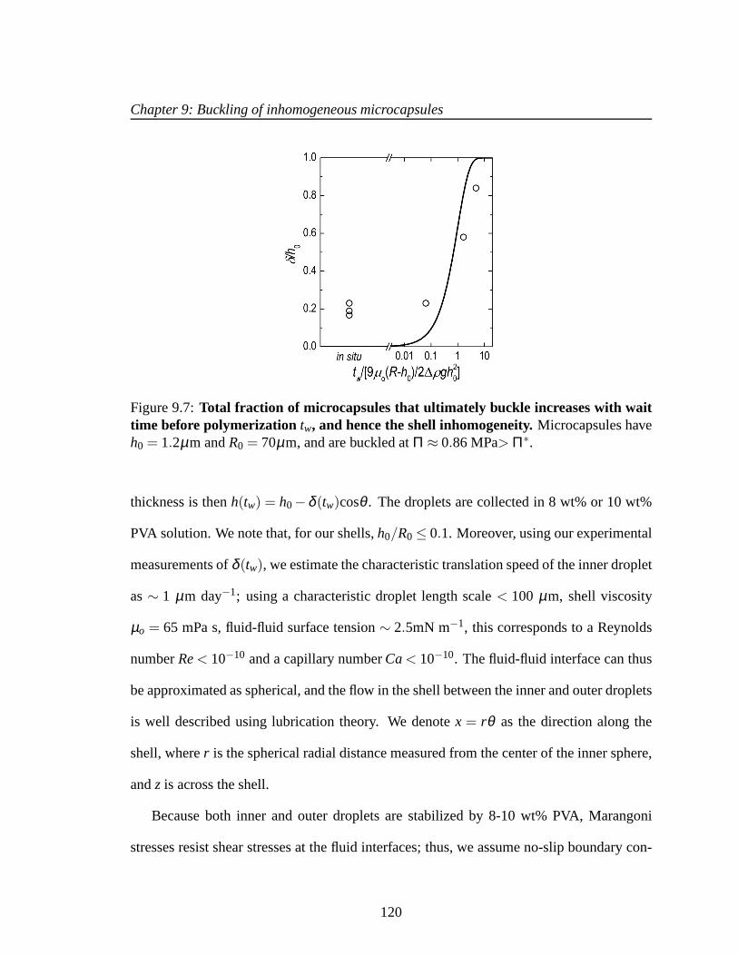
Chapter 9: Buckling of inhomogeneous microcapsules
Figure 9.7:Total fraction of microcapsules that ultimately buckle increases with waittime before polymerization tw, and hence the shell inhomogeneity.Microcapsules haveh0 = 1.2µm andR0 = 70µm, and are buckled atΠ ≈ 0.86 MPa> Π∗.
thickness is thenh(tw) = h0−δ (tw)cosθ . The droplets are collected in 8 wt% or 10 wt%
PVA solution. We note that, for our shells,h0/R0 ≤ 0.1. Moreover, using our experimental
measurements ofδ (tw), we estimate the characteristic translation speed of the inner droplet
as∼ 1 µm day−1; using a characteristic droplet length scale< 100 µm, shell viscosity
µo = 65 mPa s, fluid-fluid surface tension∼ 2.5mN m−1, this corresponds to a Reynolds
numberRe< 10−10 and a capillary numberCa< 10−10. The fluid-fluid interface can thus
be approximated as spherical, and the flow in the shell between the inner and outer droplets
is well described using lubrication theory. We denotex = rθ as the direction along the
shell, wherer is the spherical radial distance measured from the center ofthe inner sphere,
andz is across the shell.
Because both inner and outer droplets are stabilized by 8-10wt% PVA, Marangoni
stresses resist shear stresses at the fluid interfaces; thus, we assume no-slip boundary con-
120

Chapter 9: Buckling of inhomogeneous microcapsules
ditions on the fluid-fluid interfaces atz = 0 andz = h(θ , tw). The Stokes equation then
yields the velocity distribution:
ux(θ ,z, tw) =1
2µ(R0−h0)
∂ p∂θ
z(z−h(θ , tw)) (9.3)
Integrating the continuity equation twice across the gap, with ur = 0 at the outer bound-
ary,ur = Ucosθ at the inner translating boundary, anduθ = ux = 0 at both boundaries, we
find the pressure distribution
p(θ , tw) = p0(tw)− 3µo(R0−h0)2U
δh2 (9.4)
Balancing forces in thezdirection, 2π∫ π
θ=0 pn ·ez sinθdθ = Fb, whereFb≡ (4/3)π(R0−
h0)3∆ρg is the buoyant force on the inner sphere and∆ρ is the difference in density be-
tween the inner and outer spheres (0.08 g/cm3). We complete the integral and substitute
U = ∂δ/∂ tw, and take the limitδ/h0 → 1 [318]; we obtain
1h0−δ
∂δ∂ tw
=Fbh2
0
6πµo(R0−h0)4 =⇒ δ (tw)
h0= 1 − e
− 2∆ρgh20tw
9µo(R0−h0) (9.5)
To test this prediction, we use SEM or confocal microscopy measurements of micro-
capsules with fluorescently-labeled shells to directly measureδ/h0 for microcapsules of
varyingtw. We find good agreement between the two, particularly for largetw, whenδ/h0
precipitously rises to 1, as shown in Figure 9.7. We findδ/h0 → 0.2 astw → 0, in contrast
to the theory; this is to be expected, due to the slight bias inthe inner droplet position as
the double emulsions are formed in the microfluidics device.
We use Equation 9.5 to relate our measurements ofτ to δ/h0. Remarkably, we find
good agreement between our data and Equation 9.2, withk≈ 3.5×10⁻²⁴ m2, as shown by
the black line in Figure 9.5(f); in particular, this simple picture captures the strong decrease
121

Chapter 9: Buckling of inhomogeneous microcapsules
in τ at tw ∼ 103 s, with a shell permeability consistent with our independent measurements
[Figure 9.6]. While these results do not rule out other possible functional forms ofτ,
they further suggest that the time delay before the onset of buckling can be understood by
combining shell theory with Darcy’s law for flow through the microcapsule shell, even for
very inhomogeneous shells.
9.4 Shell inhomogeneities guide microcapsule deformations
The shell thickness inhomogeneity may continue to guide thedevelopment of defor-
mations in a microcapsule after it buckles. To explore this possibility, we use optical mi-
croscopy to monitor the evolution of the microcapsule morphologies after the onset of
buckling. Slightly inhomogeneous microcapsules typically buckle through the sudden for-
mation of a single circular indentation. As this indentation grows over time, its perimeter
eventually sharpens into straight ridges connected by 2-3 vertices [283, 291, 319]; this
folding pathway is exemplified by microcapsules polymerized in situ, characterized by
δ/h0 ≈ 0.2, as shown in Figure 9.8(a). This sharpening reflects the unique physics of thin
shells: because it is more difficult to compress the microcapsule shell than it is to bend it,
localizing compressive deformations only along sharp lines and points on the microcap-
sule surface requires less energy than uniformly compressing the shell [257]. Interesting
differences arise for very inhomogeneous microcapsules polymerized aftertw = 1 day, char-
acterized byδ/h0 ≈ 0.84. The initial folding pathway is similar; however, the perimeters
of the indentations formed in these microcapsules sharpen into straight ridges connected
by 4-5 vertices, more than in the slightly inhomogeneous case, as shown in Figure 9.8(b).
Moreover, surprisingly, roughly 30% of the very inhomogeneous microcapsules begin to
122
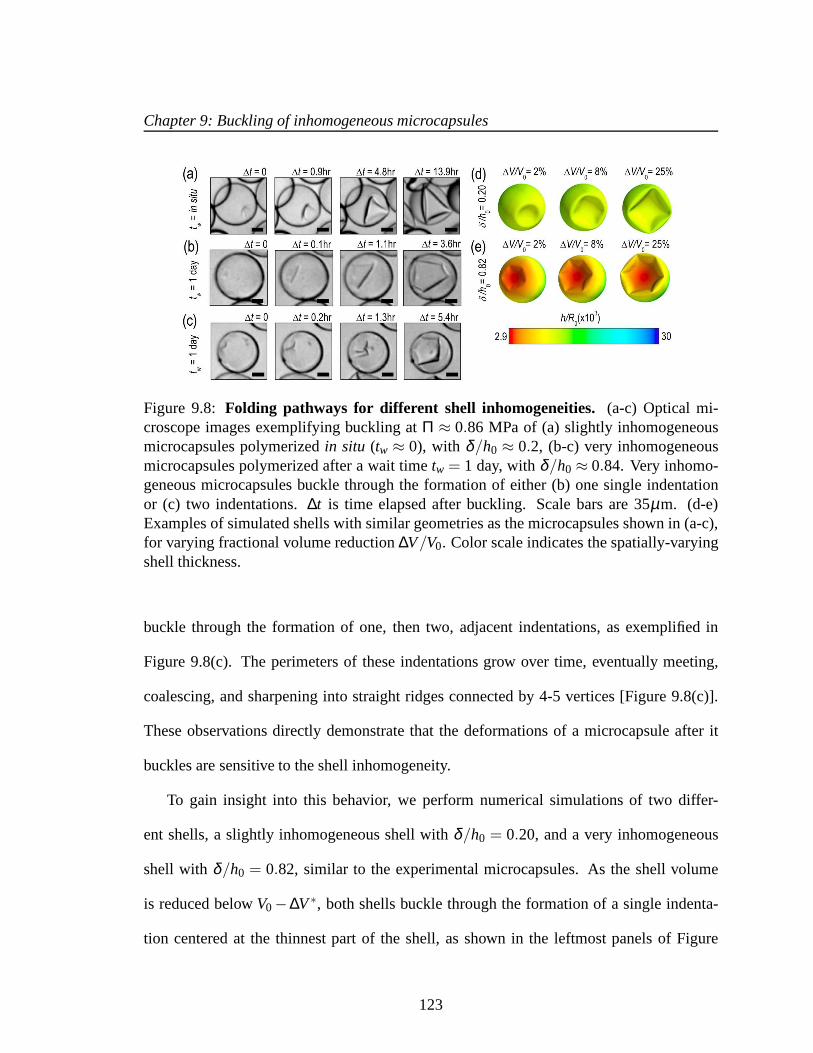
Chapter 9: Buckling of inhomogeneous microcapsules
Figure 9.8: Folding pathways for different shell inhomogeneities. (a-c) Optical mi-croscope images exemplifying buckling atΠ ≈ 0.86 MPa of (a) slightly inhomogeneousmicrocapsules polymerizedin situ (tw ≈ 0), with δ/h0 ≈ 0.2, (b-c) very inhomogeneousmicrocapsules polymerized after a wait timetw = 1 day, withδ/h0 ≈ 0.84. Very inhomo-geneous microcapsules buckle through the formation of either (b) one single indentationor (c) two indentations.∆t is time elapsed after buckling. Scale bars are 35µm. (d-e)Examples of simulated shells with similar geometries as themicrocapsules shown in (a-c),for varying fractional volume reduction∆V/V0. Color scale indicates the spatially-varyingshell thickness.
buckle through the formation of one, then two, adjacent indentations, as exemplified in
Figure 9.8(c). The perimeters of these indentations grow over time, eventually meeting,
coalescing, and sharpening into straight ridges connectedby 4-5 vertices [Figure 9.8(c)].
These observations directly demonstrate that the deformations of a microcapsule after it
buckles are sensitive to the shell inhomogeneity.
To gain insight into this behavior, we perform numerical simulations of two differ-
ent shells, a slightly inhomogeneous shell withδ/h0 = 0.20, and a very inhomogeneous
shell with δ/h0 = 0.82, similar to the experimental microcapsules. As the shellvolume
is reduced belowV0−∆V∗, both shells buckle through the formation of a single indenta-
tion centered at the thinnest part of the shell, as shown in the leftmost panels of Figure
123

Chapter 9: Buckling of inhomogeneous microcapsules
Figure 9.9:Designing lock-and-key colloids.Microcapsules with two or three sphericalinterior compartments, schematized in left panels, buckleat “weak spots” (arrows). Thisforms shapes with two or three equally-spaced circular indentations after buckling (rightpanels). Scale bars are 100µm.
9.8(d-e). As∆V increases, this indentation grows and its edges sharpen. Wefind that the
indentations formed in the very inhomogeneous shells beginto sharpen at smaller∆V/V0,
and ultimately develop more vertices than those formed in more homogeneous shells [Fig-
ure 9.8(d-e)]. These results qualitatively agree with our experimental observations [Figure
9.8(a-c)], further confirming that after the onset of buckling, the folding pathway of a shell
depends on the inhomogeneity. However, in contrast to the experimental microcapsules
[Figure 9.8(c)], we do not systematically observe the formation of adjacent indentations
in the simulations on very inhomogeneous shells. This presents a puzzle requiring further
inquiry.
Our microcapsules may be used to guide colloidal self-assembly; for example, a col-
loidal particle can spontaneously bind to the indentation formed during buckling through
a lock-and-key mechanism [320]. This mechanism is typically applied to a homogeneous
colloidal particle, which buckles through the formation ofa single indentation at a random
position on its surface. We apply our findings to create multiply-indented microcapsules
having two-fold or three-fold symmetry. To do this, we form double emulsions with two or
three inner droplets of radii larger than half the radius of the outer droplet. Consequently,
124

Chapter 9: Buckling of inhomogeneous microcapsules
the inner droplets pack closely to form dimers or trimers [321], as shown schematically in
Figure 9.9. The double emulsions are then polymerized, forming solid microcapsules with
two or three spherical compartments in their interiors, andtwo or three equally-spaced
“weak spots” in the microcapsule shell [arrows in Figure 9.9]. When exposed to a suffi-
ciently large osmotic pressure, these microcapsules buckle through the formation of multi-
ple, equally-spaced indentations at the weak spots, as shown in Figure 9.9. This approach
is thus a versatile way to create microcapsules of desired symmetries, and extends the range
of structures that can be used for lock-and-key colloidal assembly.
Our results may be applicable to other thin, spherical shells, such as biological cells
[322, 323], pollen grains [285], submersibles [324], chemical storage tanks [325], nuclear
containment shells [325], and even the earth’s crust [326]. Indeed, many of these shells are
inhomogeneous, similar to the microcapsules described here [285, 327, 328, 329, 330].
125

Chapter 10
Expansion and rupture of pH-responsive
microcapsules
One common way of characterizing the mechanical propertiesof a microcapsule is to
monitor how it responds to forces exerted on its shell. Thesecan be mechanical forces,
externally imposed by poking, squeezing, or uniformly pressurizing the microcapsule, as
described in the previous Chapter [331, 332, 333, 5]. Alternatively, these forces can arise
through physico-chemical modifications to the shell itself, such as charging it; under certain
conditions, the repulsion between the charges on the shell can cause it to deform. Electro-
static forces arise in many applications of soft matter, andconsequently, this approach is
frequently used to induce deformations in a variety of bulk materials [334, 335]. Neverthe-
less, systematic investigations of how electrostatic forces deform microcapsules are scarce
[336, 337, 338]. Thus, despite the prevalence of these forces in many real-world situations,
a full understanding of how they affect microcapsules is lacking.
126

Chapter 10: Expansion and rupture of pH-responsive microcapsules
In this Chapter9, we study the deformations of spherical microcapsules exposed to a pH
stimulus. We choose NaOH as the stimulus; when exposed to this base, the microcapsule
shells become highly charged. For large NaOH concentrations, the microcapsules expand
isotropically. We find that the extent of the microcapsule expansion can be understood
by coupling electrostatics with shell theory; moreover, the dynamics of this expansion is
well described by Darcy’s law for flow through the porous microcapsule shell. Surpris-
ingly, below a threshold NaOH concentration, the microcapsules begin to disintegrate, and
eventually rupture; they then expand non-uniformly, ultimately forming large, jellyfish-like
structures. Our results thus highlight the rich behavior exhibited by microcapsules under
the influence of electrostatic forces.
We first describe the production of microcapsules composed solely of a pH-responsive
polymer; when exposed to a trigger pH, this shell dissolves at a constant rate, ultimately
releasing the microcapsule contents. In the next section, we describe the production of
hybrid microcapsules with shells composed of a mixture of a pH-responsive and a pH-
unresponsive polymer. These microcapsules do not dissolvewhen exposed to a trigger pH,
but instead, become highly charged. We then use these hybridmicrocapsules to study how
electrostatic forces can be used to deform spherical microcapsules.
9Based on “Expansion and rupture of pH-responsive microcapsules”,S. S. Datta∗, A. Abbaspourrad∗, andD. A. Weitz, submitted,Materials Horizons(2013) and “Controlling release from pH-responsive microcap-sules”, A. Abbaspourrad∗, S. S. Datta∗, and D. A. Weitz, submitted,Langmuir(2013) *Equal contribution.
127

Chapter 10: Expansion and rupture of pH-responsive microcapsules
10.1 Microcapsules composed solely of a pH-responsive
polymer
We use a glass capillary microfluidic device to prepare monodisperse W/O/W double
emulsion drops as templates to form microcapsules [339]. The device consists of two ta-
pered cylindrical capillaries inserted into the opposite ends of a square capillary, whose
inner dimension is slightly larger than the outer diameter of the cylindrical capillaries, as
illustrated by the optical micrograph in Figure 10.1(a). This configuration enables us to ac-
curately align both cylindrical capillaries. We use the left cylindrical capillary to inject the
innermost aqueous phase, a 5 wt% aqueous solution of polyvinyl alcohol (PVA) of molec-
ular weight 13,000-23,000, seeded with a small amount of 6 nm-diameter quantum dots for
flow visualization. We treat this capillary with n-octadecyl trimethoxy silane; this renders
its surface hydrophobic, preventing wetting of the aqueousphase on the capillary wall. To
fabricate solid microcapsules, we use a middle oil phase comprised of a 5-15 wt% solu-
tion of an anionic diblock copolymer of methacrylic acid andmethyl methacrylate (PAA-b-
PMMA) in a mixture of 70 vol% chloroform and 30 vol% tetrahydrofuran (THF)[340]. We
inject this oil from the left, forcing it to flow in the same direction as the inner aqueous
phase, through the interstices between the left cylindrical capillary and the square capil-
lary. The outermost aqueous phase is a 10 wt% aqueous solution of PVA containing 15
wt% THF; we inject it from the right, forcing it to flow in the opposite direction, through
the interstices between the right cylindrical capillary and the square capillary. We operate
this hydrodynamic focusing geometry in the dripping regime, causing the inner and middle
phases to break up at the orifice of the right cylindrical capillary; this forms monodisperse
128

Chapter 10: Expansion and rupture of pH-responsive microcapsules
Figure 10.1:Microcapsules produced using microfluidics.(a) Optical micrograph of aglass capillary microfluidic device as it produces monodisperse double emulsions. Scalebar is 250µm. (b) Scanning electron microscope micrograph of monodisperse, uniform,solid microcapsules formed after evaporation of the solvent from the middle phase of thedouble emulsion drops. Scale bar is 100µm.
W/O/W double emulsions, as shown in Figure 10.1(a).
We use the right cylindrical capillary to collect these double emulsion drops; this cap-
illary is treated with 2-(methoxy(polyethyleneoxy)propyl) trimethoxy silane, rendering its
surface hydrophilic and preventing wetting of the middle oil phase on the capillary wall.
After the double emulsion drops are collected, the solvent in the middle oil phase slowly
diffuses into the outer continuous phase; this forces the PAA-b-PMMA to precipitate.
Within one hour, this forms a uniform solid shell of radius≈ 69µm, as exemplified in Fig-
ure 10.1(b). We wash the monodisperse microcapsules thus formed with water, adjusted to
have pH = 6, three times to remove any surfactant from the continuous phase.
The resulting microcapsules stably encapsulate their contents over at least 30 days;
however, when exposed to a basic pH> 7, the polymer chains making up the shells be-
come highly charged and repel each other [340]. This causes the microcapsule shells to
dissolve at a constant rate, starting at their exteriors; after a time delay of several minutes,
129

Chapter 10: Expansion and rupture of pH-responsive microcapsules
Figure 10.2:pH-triggered release from microcapsules.Optical micrographs showingthe degradation of the 500 nm-thick shell of a microcapsule,leading to the release of anencapsulated dye starting at 12 min (green; fluorescence micrograph superimposed). Themicrocapsules also encapsulate, and subsequently release, polystyrene particles used forenhanced visualization (grey). Scale bar is 100µm. Time stamp shows time elapsed afterpH is raised to 9.
the shells become fully dissolved, and the microcapsules release their contents, as shown
in Figure 10.2. We expect microcapsules with thicker shellsto take longer to fully dissolve
and ultimately release their contents; thus, to control thetime of release, we exploit the
precise flow control afforded by microfluidics to prepare microcapsules of the same outer
radius, but with different shell thicknesses. We do this by varying the flow rates of the inner
and middle phases,Qi andQm, respectively, while maintaining their sum, and the flow rate
of the outer phase,Qo, at constant values of 1.2 mL/hr and 6.0 mL/hr, respectively. Cru-
cially, the thickness of the middle phase of each double emulsion drop, and consequently,
the thickness of the solid shell formed from it, increases with increasingQm/Qi , as shown
in Figure 10.3(a). To quantify the release kinetics for microcapsules of different shell thick-
nesses, we monitor individual microcapsules using fluorescence microscopy, measuring the
time between initiation of a trigger through exposure to a pH= 9 and the beginning of the
release from their interiors [341]. The time delay increases linearly with increasing shell
thickness, varying from just a minute up to tens of minutes, as shown in Figure 10.3(b);
this is consistent with our expectation.
130

Chapter 10: Expansion and rupture of pH-responsive microcapsules
By fabricating and mixing varying amounts of different populations of capsules, each
characterized by a different shell thickness, we can precisely control the distribution of
release times over a range spanning one minute to nearly one hour. This enables us to
program sequential release from different microcapsules;to illustrate this, we fabricate
and mix two different populations of microcapsules, havingeither thin 500 nm shells or
thick 4µm shells. We distinguish the two populations by encapsulating a green and a red
dye within the microcapsules having thin and thick shells, respectively [first frame, Figure
10.4]. We increase the pH of the continuous phase to 9, forcing the shells to dissolve.
After two minutes, the microcapsules with thin shells release their contents; in contrast, the
microcapsules with thicker shells continue to stably encapsulate their contents, as shown in
the second and third frames of Figure 10.4. These subsequently release their contents after
thirteen more minutes have passed, as shown in the last two frames of Figure 10.4. These
results demonstrate that varying the microcapsule shell thickness provides a straightforward
means of programming sequential release at different times.
This experimental approach can be used to trigger release ata range of different pH
conditions. To illustrate its generality, we apply the samemicrofluidic device, but use a dif-
ferent middle oil phase; this enables us to prepare microcapsules that release their contents
under acidic conditions. The oil phase is an 8 wt% solution ofa cationic triblock copolymer
of poly-(n-butyl methacrylate-(2-dimethylaminoethyl)-methacrylate-methyl methacrylate)
(DMAEMA-BMA-MMA) in a mixture of 70 vol% chloroform and 30 vol% THF [342].
Similar to the previous case, after the double emulsion drops are formed and collected, the
solvent in the middle oil phase slowly diffuses into the continuous phase; this forces the
polymer to precipitate, forming a uniform solid shell. In contrast to the PAA-b-PMMA
131

Chapter 10: Expansion and rupture of pH-responsive microcapsules
Figure 10.3:Controlling shell geometry using microfluidics. (a) Ratio of microcapsuleshell thickness to shell radius, measured using scanning electron microscopy, increaseswith increasing ratio of middle phase flow rateQm to inner phase flow rateQi . Examplescanning electron micrographs for thin and thick shells areshown in the inset. (b) Timedelay before release begins, quantified using fluorescence microscopy of microcapsules en-capsulating a fluorescent dye, increases with increasing shell thickness, for shells triggeredat pH = 9; grey line shows linear relationship. Vertical error bars show standard devia-tion in measured release time, while horizontal error bars show standard deviation in shellthickness of each batch.
case, however, the DMAEMA-BMA-MMA polymer chains become highly charged only
under acidic conditions; consequently, the microcapsule shells thus formed dissolve and
release their contents only for pH< 6 [343, 344]. We are therefore able to prepare micro-
capsules that very stably encapsulate their contents, and only release them when exposed
to either acidic or basic conditions.
This experimental approach enables us to program the sequential release of different ac-
tives upon exposure to different pH conditions; to illustrate this, we fabricate and mix two
different populations of acid-responsive and base-responsive microcapsules. We distin-
guish the two populations by encapsulating a green dye within the base-responsive PAA-b-
PMMA microcapsules, and a yellow dye, along with 1µm polystyrene particles, within the
acid-responsive DMAEMA-BMA-MMA microcapsules [first frame, Figure 10.5]. Both
132

Chapter 10: Expansion and rupture of pH-responsive microcapsules
Figure 10.4:Controlling time of release. Optical micrographs showing the release, start-ing at 2 min, of an encapsulated dye from microcapsules with 500 nm-thick shells (green;fluorescence micrograph superimposed). A second encapsulated dye is then released, start-ing at 15 min, from microcapsules with 4µm-thick shells (red; fluorescence micrographsuperimposed). Scale bar is 250µm. Time stamp shows time elapsed after pH is raised to9.
populations of microcapsules are stable in water adjusted to have pH = 6.5. We then de-
crease the pH of the continuous phase to 5; while the base-responsive microcapsules remain
stable, the acid-responsive microcapsules quickly release their contents, as shown in the
second and third frames of Figure 10.5. We subsequently increase the pH of the continuous
phase to 9; this forces the base-responsive microcapsules to also release their contents, as
shown in the last two frames of Figure 10.5. These observations demonstrate that vary-
ing the microcapsule shell composition provides a straightforward means of programming
sequential release at different pH.
10.2 Hybrid microcapsules
We fabricate monodisperse thin-shelled microcapsules using water-in-oil-in-water (W/O/W)
double emulsion templates prepared by microfluidics [339]. The inner and outer phases are
6 wt % and 10 wt % solutions of polyvinyl alcohol (PVA), respectively, while the middle oil
phase is a mixture of a pH-responsive polymer, suspended in tetrahydrofuran (THF), and
another photo-polymerizable pH-unresponsive monomer. Weuse UV light to polymerize
133
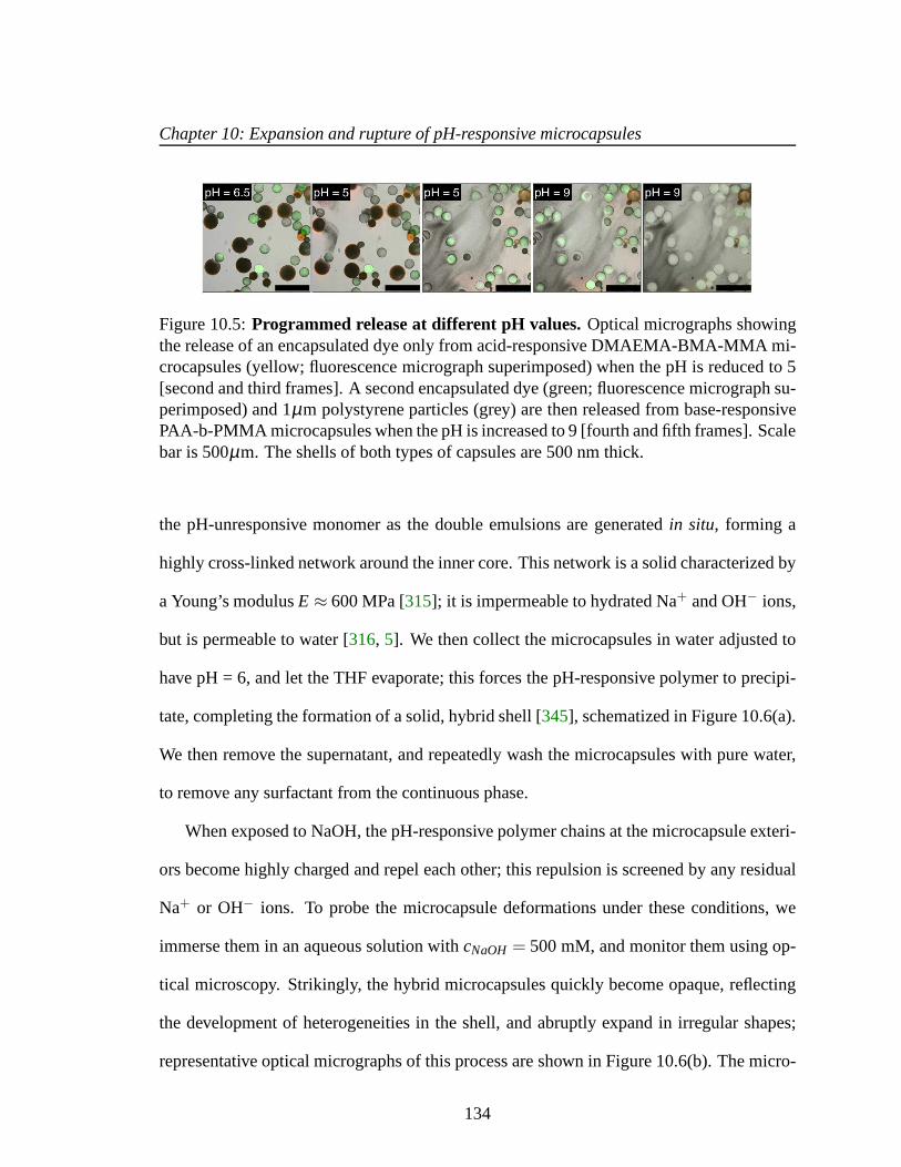
Chapter 10: Expansion and rupture of pH-responsive microcapsules
Figure 10.5:Programmed release at different pH values.Optical micrographs showingthe release of an encapsulated dye only from acid-responsive DMAEMA-BMA-MMA mi-crocapsules (yellow; fluorescence micrograph superimposed) when the pH is reduced to 5[second and third frames]. A second encapsulated dye (green; fluorescence micrograph su-perimposed) and 1µm polystyrene particles (grey) are then released from base-responsivePAA-b-PMMA microcapsules when the pH is increased to 9 [fourth and fifth frames]. Scalebar is 500µm. The shells of both types of capsules are 500 nm thick.
the pH-unresponsive monomer as the double emulsions are generatedin situ, forming a
highly cross-linked network around the inner core. This network is a solid characterized by
a Young’s modulusE ≈ 600 MPa [315]; it is impermeable to hydrated Na+ and OH− ions,
but is permeable to water [316, 5]. We then collect the microcapsules in water adjusted to
have pH = 6, and let the THF evaporate; this forces the pH-responsive polymer to precipi-
tate, completing the formation of a solid, hybrid shell [345], schematized in Figure 10.6(a).
We then remove the supernatant, and repeatedly wash the microcapsules with pure water,
to remove any surfactant from the continuous phase.
When exposed to NaOH, the pH-responsive polymer chains at the microcapsule exteri-
ors become highly charged and repel each other; this repulsion is screened by any residual
Na+ or OH− ions. To probe the microcapsule deformations under these conditions, we
immerse them in an aqueous solution withcNaOH = 500 mM, and monitor them using op-
tical microscopy. Strikingly, the hybrid microcapsules quickly become opaque, reflecting
the development of heterogeneities in the shell, and abruptly expand in irregular shapes;
representative optical micrographs of this process are shown in Figure 10.6(b). The micro-
134
Chapter 10: Expansion and rupture of pH-responsive microcapsules
capsules ultimately expand into spheres, as shown by the last frame of Figure 10.6(b); this
entire process occurs over a timescale of∼ 10 s.
We quantify this behavior by measuring the maximal expansion, γ ≡ (Rf −R0)/R0,
whereR0 andRf are the average initial and final microcapsule radii, respectively. We also
measure the average time taken for the microcapsules to expand into their final spherical
shapes,τ. To elucidate the expansion behavior, we explore even lowervalues ofcNaOH.
Intriguingly, γ increases strongly with decreasingcNaOH, as shown in the upper panel of
Figure 10.7, reaching a value exceeding 1 atcNaOH = 25 mM; the expansion timeτ con-
comitantly increases, but only weakly, as shown by the grey squares in the lower panel of
Figure 10.7. Unexpectedly, atcNaOH = 25 mM, the microcapsules also begin to disinte-
grate, forming fragments of size∼ 1 µm, as indicated by the arrows in Figure 10.6(c). At
even smallercNaOH, the microcapsules first disintegrate, as shown by the first frame of Fig-
ure 10.6(d); this ultimately results in the formation of a hole in each shell after a time delay
τ1 ∼ 10−100 s. The microcapsules then begin to intermittently expand outward, starting at
the hole perimeters, as exemplified by the last three frames of Figure 1(d); the region of the
shell that expands is indicated by the arrow in each frame. This process occurs over a time
periodτ2 ∼ 10−100 s; the expansion then stops, leaving wrinkled jellyfish-like structures,
approximately 300µm in size.
The isotropic expansion at highcNaOH ≥ 25 mM is due to the charging of the micro-
capsule shells; when exposed to NaOH, the pH-responsive polymers at the microcapsule
exteriors become highly charged, leading to a surface charge densityσ . We thus expect
that the repulsion between the charges on each spherically-symmetric shell leads to a force,
directed radially outward, on the shell. We estimate [346] the magnitude of the resultant
135

Chapter 10: Expansion and rupture of pH-responsive microcapsules
1.6 mM
25 mM
500 mM
27 s 230 s 256 s 290 s
7 s 15 s 73 s 320 s
6.6 s 7.3 s 8.6 s 12.5 s
c
d
b
aOH-
H2O
Na+
6% PVA
-
pH sensitive
polymer
inert
polymer
Figure 10.6:Expansion and rupture of microcapsules.(a) Schematic of a hybrid micro-capsule, showing the thin, solid, spherical shell composedof a pH-unresponsive polymerand a pH-responsive polymer. The core is a 6 wt% aqueous solution of polyvinyl alcohol(PVA). The pH-responsive polymer at the surface of the shellbecomes charged when ex-posed to NaOH in the continuous phase. First frame of (b) shows an optical micrographof a hybrid microcapsule after it is collected. Subsequent frames in (b), (c), and (d) showthe expansion of the microcapsule when exposed to differentNaOH concentrations. (c)At cNaOH = 25 mM, the shell begins to disintegrate, as indicated by the arrows in the lastframe. (d) For lowercNaOH < 25 mM, the shell first disintegrates, as indicated by the arrowin the first frame, then ruptures through the formation of a hole, shown in the second frame,then expands into a wrinkled jellyfish-like structure, shown in the last two frames. Scalebars indicate 100µm.
136

Chapter 10: Expansion and rupture of pH-responsive microcapsules
electrostatic pressure aspe≈σ2κ−1/εε0R, whereε ≈ 80 is the dielectric constant of water,
ε0 is the permittivity of free space,R is the time-dependent radius of the spherical micro-
capsule,κ−1 is the length over which the repulsive interactions are screened. The quantity
of NaOH required to fully charge the shell is small; consequently, the excess Na+ and OH−
ions, which screen the surface charges on the shell, have a concentration≈ cNaOH, and thus
κ−1 = A/√
cNaOH, with A≡ 0.304 nm·M1/2 [347]. As the microcapsule expands isotrop-
ically, a tensile stress builds up within its shell; this resists the expansion. We use shell
theory to estimate this stress,pm = Eh(1/R0−1/R), whereh≈ 3 µm is the average shell
thickness, measured using scanning electron microscopy [317]. We thus expect that the
microcapsules expand until the electrostatic pressure andtensile stress balance each other;
this yields a maximal expansion strainγ = σ2A/Eεε0h√
cNaOH. We test this prediction
using our measurements ofγ. We findγ ∼ c−1/2NaOH, as shown by the line in the top panel of
Figure 10.7, consistent with the theoretical prediction; fitting the experimental data yields
an estimate ofσ ≈ 300e/nm2, wheree is the charge of an electron. These results suggest
that the microcapsule expansion can be understood by coupling electrostatics with shell
theory.
Within this picture, the Na+ and OH− ions screen the repulsion between the charges on
the microcapsule shells. As an additional test of this idea,we expose the microcapsules to a
25 mM NaOH solution, also containing 500 mM NaCl; we expect the Na+ and Cl− ions to
similarly screen the repulsion between the charges on the microcapsule shells. Consistent
with our expectation, the microcapsules do not disintegrate, unlike microcapsules exposed
to only 25 mM NaOH. Instead, they expand slightly, reaching amaximal expansion strain
γ ≈ 0.4, much smaller than that expected forcNaOH. This value of the strain is instead
137
Chapter 10: Expansion and rupture of pH-responsive microcapsules
comparable to that expected forcNaOH = 525 mM, as shown by the line in the top panel of
Figure 10.7, thus confirming the validity of our picture.
The microcapsules expand to their maximal size over a time period τ. We hypothe-
size that this behavior reflects the dynamics of the fluid flow into the microcapsule cores,
through their porous shells, as they expand [5]. We estimate this inflow rate using Darcy’s
law, pe− pm = µhR/3k, whereµ ≈ 1 mPa· s is the viscosity of water andk is the shell
permeability; this yields a characteristic expansion timeτ = µR20(1+ γ)/3Ek. We use our
measurements ofτ, as well as the fit to the measurements ofγ shown in the top panel of
Figure 10.7, to directly test this prediction. We find excellent agreement between the data
and the theoretical prediction, as shown by the solid line inthe bottom panel of Figure
10.7; fitting the experimental data yields a shell permeability k ≈ 10−21 m2. The agree-
ment between the data and the theoretical prediction thus suggests that the dynamics of the
microcapsule expansion can be understood using Darcy’s law.
As cNaOH decreases, the screening lengthκ−1 increases; consequently, the stress in the
microcapsule shell increases, ultimately reachingpm = pe ≈ 10 MPa atcNaOH = 25 mM.
For even smallercNaOH, the microcapsules begin to disintegrate into∼ 1 µm fragments,
and eventually rupture. We hypothesize that, under these conditions, the stress that builds
up in the shell exceeds the stress required to fracture it. Totest this hypothesis, we estimate
the fracture stress [348] using the Griffith criterion,√
2EGc/πa≈ 6−20 MPa, whereGc ∼
0.1−1 J/m2 is the surface energy per unit area of the shell material anda ≈ 1 µm is the
characteristic size of a shell fragment, measured using optical microscopy. Interestingly,
this value is in good agreement with our estimate of the maximal stress that develops in the
shell,pm≈ 10 MPa, suggesting that the observed disintegration atcNaOH≤ 25 mM reflects
138

Chapter 10: Expansion and rupture of pH-responsive microcapsules
10−0.5
10−0.3
10−0.1
100.1
Exp
ansi
on S
trai
n
10−3
10−2
10−1
100
101
102
103
[NaOH] (M)
Tim
e (s
)
Figure 10.7:Geometry and dynamics of microcapsule expansion.(Top Panel) Maximalexpansion strain of spherical microcapsules exposed to different NaOH concentrations; lineshows theoretical prediction described in the text, withσ ≈ 300e/nm2, wheree is the ele-mentary charge. (Bottom Panel) Grey squares show time takenfor spherical microcapsulesto fully expand; line shows theoretical fit described in the text. Blue triangles and red cir-cles the time period over which the shell disintegrates before a hole forms in it,τ1, and thetime period over which the shell subsequently expands into ajellyfish-like structure,τ2,respectively, forcNaOH < 25 mM.
139
Chapter 10: Expansion and rupture of pH-responsive microcapsules
the fracturing of the microcapsule shell.
Finally, we monitor the dynamics of the disintegration, rupture, and subsequent expan-
sion of the microcapsule shell that occurs atcNaOH < 25 mM. Intriguingly, both the time
period over which the shell fractures before a hole forms in it, τ1, and the time period over
which the shell subsequently expands into a jellyfish-like structure,τ2, both increase with
decreasingcNaOH, as shown by the blue triangles and red circles in Figure 10.7, respec-
tively. A complete understanding of these dynamics remainsa puzzle requiring further
inquiry.
Our work highlights the fascinating range of structures exhibited by pH-responsive mi-
crocapsules, driven by the interplay between electrostatic and mechanical forces. Intrigu-
ingly, many of these structures are reminiscent of structures, also induced by electrostatic
effects, that are often observed in other soft matter systems, such as viruses [346, 349, 350]
and red blood cells [351].
140

Bibliography
[1] J. Bear.Dynamics of Fluids in Porous Media. Dover, 1988.
[2] W. C. Yang. Handbook of Fluidization and Fluid-Particle Systems. CRC Press,2003.
[3] J. C. Giddings.Dynamics of Chromatography. CRC Press, 2002.
[4] M. M. Mench. Fuel Cell Engines. Wiley, 2008.
[5] S. S. Datta, S. H. Kim, J. Paulose, A. Abbaspourrad, D. R. Nelson, and D. A. Weitz.Delayed buckling and guided folding of inhomogeneous capsules. Phys. Rev. Lett.,109:134302, 2012.
[6] A. R. A. Khaled and K. Vafai. The role of porous media in modeling flow and heattransfer in biological tissues.Int. J. Heat and Mass Transfer, 46:4989–5003, 2003.
[7] J. Ranft, J. Prost, F. Julicher, and J. F. Joanny. Tissue dynamics with permeation.Eur. Phys. J. E, 35:46, 2012.
[8] S. Veran-Tissoires, M. Marcoux, and M. Prat. Discrete salt crystallization at thesurface of a porous medium.Phys. Rev. Lett., 108:054502–054505, 2012.
[9] J. M. Rutkowski and M. A. Swartz. A driving force for change: interstitial flow as amorphoregulator.Trends in Cell Biol., 17:44–50, 2006.
[10] W. Rose and P. A. Witherspoon. Studies of waterflood performance II: trapping oilin a pore doublet.Ill. State Geological Survey, 224:3, 1956.
[11] E. F. Herbeck, R. C. Hemtz, and J. R. Hastings. Fundamentals of tertiary oil recov-ery. Pet. Engineer, 48:33, 1976.
[12] A. C. Payatakes. Dynamics of oil ganglia during immiscible displacement in water-wet porous media.Annu. Rev. Fluid Mech., 14:365, 1982.
[13] I. Chatzis and F. A. L. Dullien. Application of the theory of percolation for a modelof drainage in porous media and relative permeability of injected non-wetting fluids.Oil Gas Sci. Technol. Rev. IFP, 37:183, 1982.
141

Bibliography
[14] R. Lenormand, C. Zarcone, and A. Sarr. Mechanisms of thedisplacement of onefluid by another in a network of capillary ducts.J. Fluid Mech., 135:337, 1983.
[15] R. Lenormand and C. Zarcone. Role of roughness and edgesduring imbibition insquare capillaries.SPE Annual Technical Conference and Exhibition, pages SPE–13264, 1984.
[16] G. R. Jerauld and S. J. Salter. The effect of pore-structure on hysteresis in relativepermeability and capillary pressure: pore-level modeling. Transp. Porous Media,5:103, 1990.
[17] M. J. Blunt and H. Scher. Pore-level modeling of wetting. Phys. Rev. E, 52:6387,1995.
[18] M. J. Blunt, M. D. Jackson, M. Piri, and P. H. Valvatne. Detailed physics, predictivecapabilities and macroscopic consequences for pore-network models of multiphaseflow. Adv. Water Resour., 25:1069, 2002.
[19] I. Chatzis, N. R. Morrow, and H. T. Lim. Magnitude and detailed structure of residualoil saturation.Soc. Pet. Eng. J., 23:311, 1983.
[20] M. Sahimi.Flow and Transport in Porous Media and Fractured Rock. Wiley, 2012.
[21] D. Wilkinson. Percolation effects in immiscible displacement. Phys. Rev. A,34:1380, 1986.
[22] S. Sheppard, M. D. Mantle, A. J. Sederman, M. L. Johns, and L. F. Gladden. Mag-netic resonance imaging study of complex fluid flow in porous media: flow patternsand quantitative saturation profiling of amphiphilic fracturing fluid displacement insandstone cores.Magn. Reson. Imag., 21:364, 2003.
[23] M. H. Sankey, D. J. Holland, A. J. Sederman, and L. F. Gladden. Magnetic resonancevelocity imaging of liquid and gas two-phase flow in packed beds. J. Magn. Reson.,196:142, 2008.
[24] M. L. Porter, D. Wildenschild, G. Grant, and J. I. Gerhard. Measurement and predic-tion of the relationship between capillary pressure, saturation, and interfacial area ina NAPL-water-glass bead system.Water Resour. Res., 46:W08512, 2010.
[25] D. Wildenschild, R. T. Armstrong, A. L. Herring, I. M. Young, and J. W. Carey.Exploring capillary trapping efficiency as a function of interfacial tension, viscosity,and flow rate.Energy Procedia, 4:4945, 2011.
[26] S. Iglauer, S. Favretto, G. Spinelli, G. Schena, and M. J. Blunt. X-ray tomographymeasurements of power-law cluster size distributions for the non-wetting phase insandstones.Phys. Rev. E, 82:056315, 2010.
142

Bibliography
[27] M. Kumar, T. J. Senden, A. P. Sheppard, J. P. Middleton, and M. A. Knackstedt.Visualizing and quantifying the residual phase distribution in core material.Petro-physics, 51:v51n5a4, 2010.
[28] L. Lebon, L. Oger, J. Leblond, J. P. Hulin, N. S. Martys, and L. M. Schwartz. Pulsedgradient NMR measurements and numerical simulation of flow velocity distributionin sphere packings.Phys. Fluids, 8:293–301, 1996.
[29] L. Lebon, J. Leblond, and J. P. Hulin. Experimental measurement of dispersionprocesses at short times using a pulsed field gradient NMR technique.Phys. Fluids,9:481–490, 1997.
[30] D. R. Noble.Lattice Boltzmann study of the interstitial hydrodynamicsand disper-sion in steady inertial flows in large randomly packed beds. PhD thesis, Universityof Illinois and Urbana-Champaign, 1997.
[31] Olav van Genabeek.Velocity fluctuations in slow flow through porous media. PhDthesis, Massachusetts Institute of Technology, 1998.
[32] R. S. Maier, D. M. Kroll, Y. E. Kutsovsky, H. T. Davis, andR. S. Bernard. Simulationof flow through bead packs using the lattice Boltzmann method. Phys. Fluids, 10:60–74, 1998.
[33] R. S. Maier, D. M. Kroll, H. T. Davis, and R. S. Bernard. Simulation of flow inbidisperse sphere packings.J. Coll. Int. Sci., 217:341–347, 1999.
[34] L. Talon, J. Martin, N. Rakotomalala, D. Salin, and Y. C.Yortsos. Lattice BGKsimulations of macrodispersion in heterogeneous porous media. Water Resour. Res.,39:1135–1141, 2003.
[35] E. Zaman and P. Jalali. On hydraulic permeability of random packs of monodispersespheres: Direct flow simulations versus correlations.Physica A, 389:205–214, 2010.
[36] N. S. Martys, S. Torquato, and D. P. Bentz. Universal scaling of fluid permeabilityfor sphere packings.Phys. Rev. E, 50:403–408, 1994.
[37] F. M. Auzerais, J. Dunsmuir, B. B. Ferreol, N. Martys, J.Olson, T. S. Ramakrishnan,D. H. Rothman, and L. M. Schwartz. Transport in sandstone: A study based on threedimensional microtomography.Geophys. Res. Lett., 23:705–708, 1996.
[38] A. E. Scheidegger.The physics of flow through porous media. University of Torontopress, 1974.
[39] G. De Josselin de Jong. Longitudinal and transverse diffusion in granular deposits.Trans. Amer. Geophys. Union, 39:67–74, 1958.
143

Bibliography
[40] P. G. Saffman. A theory of dispersion in a porous medium.J. Fluid Mech., 6:321–349, 1959.
[41] J. Sheng.Modern Chemical Enhanced Oil Recovery: Theory and Practice. GulfProfessional Publishing, 2010.
[42] S. P. Friedman and Y. Mualem. Diffusion of fertilizers from controlled releasesources, uniformly distributed in soil.Fert. Res., 39:19, 1994.
[43] K. Tsuji. Microencapsulation of pesticides and their improved handling safety.J.Microencapsul., 18:137, 2001.
[44] K. Hirech, S. Payan, G. Carnelle, L. Brujes, and J. Legrand. Microencapsulation ofan insecticide by interfacial polymerisation.Powder Technol., 130:324, 2003.
[45] C. C. Dowler, O. D. Dailey, and B. G. Mullinix. Polymericmicrocapsules of alachlorand metolachlor: preparation and evaluation of controlled-release properties.J.Agric. Food Chem., 47:2908, 1999.
[46] T. Takei, M. Yoshida, K. Yanagi, Y. Hatate, K. Shiomori,and S. Kiyoyama. Prepa-ration of acetamiprid-loaded polymeric microcapsules: Influence of preparationparameter in emulsion system on microcapsule characteristics. Polymer Bulletin,61:119, 2008.
[47] S. Riyajan and J. T. Sakdapipanich. Development of a controlled release neem cap-sule with a sodium alginate matrix, crosslinked by glutaraldehyde and coated withnatural rubber.Polymer Bulletin, 63:609, 2009.
[48] M. A. Augustin and Y. Hemar. Nano- and micro-structuredassemblies for encapsu-lation of food ingredients.Chem. Soc. Rev., 38:902, 2009.
[49] A. Madene, M. Jacquot, J. Scher, and S. Desobry. Flavourencapsulation and con-trolled release – a review.Int. J. Food Sci. Technol., 41:1, 2006.
[50] D. J. McClements, Decker E. A, and J. Weiss. Emulsion-based delivery systems forlipophilic bioactive components.J. Food Sci., 72:109, 2007.
[51] R. Wegmueller, M. B. Zimmermann, V. G. Buhe, E. J. Windhab, and R. F. Hurrell.Development, stability, and sensory testing of microcapsules containing iron, iodine,and vitamin a for use in food fortification.J. Food Sci., 71:2, 2006.
[52] B. G. De Geest, C. De Jugnat, E. Verhoeven, G. B. Sukhorukov, A. M. Jonas, J. Plain,J. Demeester, and S. C. De Smedt. Layer-by-layer coating of degradable microgelsfor pulsed drug delivery.J. Controlled Release, 116:159, 2006.
144

Bibliography
[53] G. Ibarz, L. Dahne, E. Donath, and H. Mohwald. Smart micro- and nanocontainersfor storage, transport, and release.Adv. Mater., 13:1324, 2001.
[54] S. Ye, C. Wang, X. Liu, Z. Tong, B. Ren, and F. Zeng. New loading process andrelease properties of insulin from polysaccharide microcapsules fabricated throughlayer-by-layer assembly.J. Controlled Release, 112:79, 2006.
[55] H. Ai, S. A. Jones, M. M. Villiers, and Y. M. Lvov. Nano-encapsulation offurosemide microcrystals for controlled drug release.J. Controlled Release, 86:59,2003.
[56] S. H. Hu, C. H. Tsai, C. F. Liao, D. M. Liu, and S. Y. Chen. Controlled ruptureof magnetic polyelectrolyte microcapsules for drug delivery. Langmuir, 24:11811,2008.
[57] D. G. Shchukin, D. A. Gorin, and H. Mohwald. Ultrasonically induced opening ofpolyelectrolyte microcontainers.Langmuir, 22:7400, 2006.
[58] B. G. De Geest, A. G. Skirtach, A. A. Mamedov, A. A. Antipov, N. A. Kotov,S. C. De Smedt, and G. B. Sukhorukov. Ultrasound-triggered release from mul-tilayered capsules.Small, 3:804, 2007.
[59] C. H. Choi, J. H. Jung, D. W. Kim, Y. M. Chung, and C. S. Lee.Novel one-potroute to monodisperse thermosensitive hollow microcapsules in a microfluidic sys-tem. Lab on a Chip, 8:1544, 2008.
[60] T. He, K. Zhang, X. Mu, T. Luo, Y. Wang, and G. Luo. A modified microfluidicchip for fabrication of paclitaxel-loaded poly(l-lactic acid) microspheres.Microfluid.Nanofluid., 10:1289, 2011.
[61] R. Karnik, F. Gu, P. Basto, C. Cannizzaro, L. Dean, W. Kyeimanu, R. Langer,and O. C. Farokhzad. Microfluidic platform for controlled synthesis of polymericnanoparticles.Nano Lett., 8:2906, 2008.
[62] S. Leclercq, K. R. Harlander, and G. A. Reineccius. Formation and characterizationof microcapsules by complex coacervation with liquid or solid aroma cores.Flavourand Fragrance Journal, 24:17, 2008.
[63] K. Miyazawa, I. Yajima, I. Kaneda, and T. Yanaki. Preparation of a new soft capsulefor cosmetics.J. Cosmet. Sci., 51:239, 2000.
[64] M. Jacquemond, N. Jeckelmann, L. Ouali, and O. P. Haefliger. Perfume-containingpolyurea microcapsules with undetectable levels of free isocyanates.J. Appl. Poly-mer Sci., 114:3074, 2009.
145
Bibliography
[65] T. Feczko, V. Kokol, and B. Voncina. Preparation and characterization ofethylcellulose-based microcapsules for sustaining release of a model fragrance.Macromolecular Research, 18:636, 2010.
[66] R. Badulescu, V. Vivod, D. Jausovec, and B. Voncina. Grafting of ethylcellulosemicrocapsules onto cotton fibers.Carbohyd. Polym., 71:85, 2008.
[67] G. Orive, R. M. Hernandez, A. R. Gascon, R. Calafiore, T. M. S. Chang, P. de Vos,G. Hortelano, D. Hunkeler, I. Lacik, A. M. Shapiro, and J. L. Pedraz. Cell encapsu-lation: promise and progress.Nat. Med., 9:104, 2003.
[68] N. C. Hunt and L. M. Grover. Cell encapsulation using biopolymer gels for medicalapplications.Biotechnol. Lett., 32:733, 2010.
[69] T. Joki, M. Machluf, A. Atala, J. Zhu, N. T. Seyfried, I. F. Dunn, T. Abe, and R. S.Carroll. Continuous release of endostatin from microencapsulated engineered cellsfor tumor therapy.Nat. Biotechnol., 19:35, 2001.
[70] T. M. S. Chang. Therapeutic applications of polymeric artificial cells. Nat. Rev.Drug Discov., 4:221, 2005.
[71] T. Vermonden, N. E. Fedorovich, D. van Geemen, J. Alblas, C. F. van Nostrum,W. J. A. Dhert, and W. E. Hennink. Photopolymerized thermosensitive hydrogels:synthesis, degradation, and cytocompatibility.Biomacromolecules, 9:919, 2008.
[72] H. Uludag, P. de Vos, and P. A. Tresco. Technology of mammalian cell encapsula-tion. Adv. Drug Deliv. Rev., 42:29, 2000.
[73] W. Qi, X. Yan, L. Duan, Y. Cui, Y., Yang, and J. Li. Glucose-sensitive microcap-sules from glutaraldehyde cross-linked hemoglobin and glucose oxidase.Biomacro-molecules, 10:1212, 2009.
[74] M. J. McShane, J. Q. Brown, K. B. Guice, and Y. M. Lvov. Polyelectrolyte mi-croshells as carriers for fluorescent sensors: loading and sensing properties of aruthenium-based oxygen indicator.Nanoscience and Nanotechnology, 2:411, 2002.
[75] L. I. Kazakova, L. I. Shabarchina, and G. B. Sukhorukov.Co-encapsulation of en-zyme and sensitive dye as a tool for fabrication of microcapsule based sensor forurea measuring.Phys. Chem. Chem. Phys., 13:11110, 2011.
[76] L. E. Sinks, G. P. Robbins, E. Roussakis, T. Troxler, D. A. Hammer, and S. A.Vinogradov. Two-photon microscopy of oxygen: polymersomes as probe carriervehicles.J. Phys. Chem. B, 114:14373, 2010.
[77] S. L. Poe, M. Kobaslija, and D. T. McQuade. Mechanism andapplication of amicrocapsule enabled multicatalyst reaction.J. Am. Chem. Soc., 129:9216, 2007.
146

Bibliography
[78] C. Ramaraoa, S. V. Ley, S. C. Smith, I. M. Shirley, and N. DeAlmeidac. Polyureaencapsulated palladium acetate: a robust and recyclable catalyst for use in conven-tional and supercritical media.Chem. Commun., 13:1132, 2002.
[79] B. J. Blaiszik, M. M. Caruso, D. A. McIlroy, J. S. Moore, S. R. White, and N. R. Sot-tos. Microcapsules filled with reactive solutions for self-healing materials.Polymer,50:990, 2009.
[80] E. N. Brown, S. R. White, and N. R. Sottos. Microcapsule induced toughening in aself-healing polymer composite.J. Mater. Sci., 39:1703, 2004.
[81] M. A. White. The chemistry behind carbonless copy paper. J. Chem. Educ., 75:1119,1998.
[82] B. Comiskey, J. D. Albert, H. Yoshizawa, and J. Jacobson. An electrophoretic inkfor all- printed reflective electronic displays.Nature, 394:253, 1998.
[83] C. A. Kim, M. J. Joung, S. D. Ahn, G. H. Kim, S. Y. Kang, I. K.You, J. Oh, H. J.Myoung, K. H. Baek, and K. S. Suh. Microcapsules as an electronic ink to fabricatecolor electrophoretic displays.Synthetic Metals, 151:181, 2005.
[84] Y. Chen, J. Au, P. Kazlas, A. Ritenour, H. Gates, and M. McCreary. Electronicpaper: flexible active-matrix electronic ink display.Nature, 136:423, 2003.
[85] T. J. Plona. Observation of a second bulk compressionalwave in a porous mediumat ultrasonic frequencies.Appl. Phys. Lett., 36:259, 1980.
[86] K. M. Ng, H. T. Davis, and L. E. Scriven. Visualization ofblob mechanics in flowthrough porous media.Chem. Eng. Sci., 33:1009, 1978.
[87] R. J. Mannheimer and C. J. Oswald. Development of transparent porous media withpermeabilities and porosities comparable to soils, aquifers, and petroleum reservoirs.Ground Water, 31:781, 1993.
[88] M. Stohr, K. Roth, and B. Jahne. Measurement of 3D pore-scale flow in index-matched porous media.Exp. in Fluids, 35:159, 2003.
[89] P. Sharma, P. Aswathi, A. Sane, S. Ghosh, and S. Bhattacharya. Three- dimen-sional real-time imaging of bi-phasic flow through porous media. Rev. Sci. Instrum.,82:113704, 2011.
[90] T. Walmann. Visualization of transport phenomena in three-dimensional porousmedia. Master’s thesis, University of Oslo, 1992.
[91] V. Frette, J. Feder, T. Jossang, P. Meakin, and K. J. Maloy. Fast, immiscible fluid-fluid displacement in three-dimensional porous media at finite viscosity contrast.Phys. Rev. E, 50:2881, 1994.
147

Bibliography
[92] W. C. Lyons.Standard Handbook of Petroleum and Natural Gas Engineering. GulfProfessional Publishing, Oxford, 1996.
[93] Y. Gueguen and V. Palciauskas.Introduction to the Physics of Rocks. Princeton,Princeton, 1994.
[94] A. P. Philipse and C. Pathmamanoharan. Liquid permeation (and sedimentation) ofdense colloidal hard-sphere packings.J. Coll. Int. Sci., 159:96, 1993.
[95] A. T. Krummel, S. S. Datta, S. Munster, and D. A. Weitz. Visualizing multiphaseflow and trapped fluid configurations in a model three-dimensional porous medium.AIChE J., 59:1022, 2013.
[96] P. G. Toledo, L. E. Scriven, and H. T. Davis. Equilibriumand stability of staticinterfaces in biconical pore segments.SPE Form. Eval., 9:46, 1994.
[97] G. Mason and N. Morrow. Meniscus displacement curvatures of a perfectly wettingliquid in capillary pore throats formed by spheres.J. Coll. Int. Sci., 109:46, 1986.
[98] R. Lenormand and C. Zarcone. Invasion percolation in anetched network: measure-ment of a fractal dimension.Phys. Rev. Lett., 54:2229, 1985.
[99] K. J. Maloy, L. Furuberg, J. Feder, and T. Jossang. Gravity invasion percolation intwo dimensions: experiment and simulation.Phys. Rev. Lett., 68:2161, 1992.
[100] N. Martys, M. Cieplak, and M. O. Robbins. Critical phenomena in fluid invasion ofporous media.Phys. Rev. Lett., 66:1058, 1991.
[101] B. Xu, Y. C. Yortsos, and D. Salin. Invasion percolation with viscous forces.Phys.Rev. E, 57:739, 1998.
[102] L. Xu, S. Davis, A. B. Schofield, and D. A. Weitz. Dynamics of drying in 3D porousmedia.Phys. Rev. Lett., 101:094502, 2008.
[103] W. E. Galloway and D. K. Hobday.Terrigenous clastic depositional systems: appli-cations to fossil fuel and groundwater resources. Springer, New York, 1996.
[104] S. E. Gasda and M. A. Celia. Upscaling relative permeabilities in a structured porousmedium.Adv. Water Resour., 28:493, 2004.
[105] H. Hoteit and A. Firoozabadi. Numerical modeling of two-phase flow in hetero-geneous permeable media with different capillarity pressures. Adv. Water Resour.,31:56, 2008.
[106] B. H. Keuper and E. O. Frind. Two-phase flow in heterogeneous porous media: 1.Model development.Water Resour. Res., 27:1049, 1991.
148

Bibliography
[107] G. F. Pinder and W. G. Gray.Essentials of multiphase flow and transport in porousmedia. Wiley, 2008.
[108] N. Shokri, P. Lehmann, and D. Or. Evaporation from layered porous media.J.Geophys. Res., 115:B06204, 2010.
[109] J. A. Neufeld and H. E. Huppert. Modelling carbon dioxide sequestration in layeredstrata.J. Fluid Mech., 625:353, 2009.
[110] H. M. Selim and L. Ma.Physical nonequilibrium in soils: modeling and application.Ann Arbor Press, Chelsea, 1998.
[111] M. Romano, M. Chabert, A. Cuenca, and H. Bodiguel. Strong influence of geomet-rical heterogeneity on drainage in porous media.Phys. Rev. E, 84:065302, 2011.
[112] K. K. Mohanty, H. T. Davis, and L. E. Scriven. Physics ofoil entrapment in water-wet rock.SPE Reservoir Engineering, 2:113, 1987.
[113] R. Al Raoush.Extraction of physically-realistic pore network properties from three-dimensional synchrotron microtomography images of unconsolidated porous media.PhD thesis, Louisiana State University, 2002.
[114] K. E. Thompson, C. S. Willson, C. D. White, S. Nyman, J. Bhattacharya, and A. H.Reed. Application of a new grain-based reconstruction algorithm to microtomogra-phy images for quantitative characterization and flow modeling. SPE, 95887, 2005.
[115] J. P. Stokes, D. A. Weitz, J. P. Gollub, A. Dougherty, M.O. Robbins, P. M. Chaikin,and H. M. Lindsay. Interfacial stability of immiscible displacement in a porousmedium.Phys. Rev. Lett., 57:1718, 1986.
[116] T. S. Ramakrishnan and D. T. Wasan. Two-phase distribution in porous media: Anapplication of percolation theory.Int. J. Multiphase Flow, 12:357, 1986.
[117] C. E. Diaz, I. Chatzis, and F. A. L. Dullien. Simulationof capillary pressure curvesusing bond correlated site percolation on a simple cubic network. Transp. PorousMedia, 2:215, 1987.
[118] M. J. Blunt, M. J. King, and H. Scher. Simulation and theory of two-phase flow inporous media.Phys. Rev. A, 46:7680, 1992.
[119] M. J. Blunt. Pore level modeling of the effects of wettability. SPE J., 2:70, 1997.
[120] M. J. Blunt. Physically-based network modeling of multiphase flow in intermediate-wet porous media.J. Pet. Sci. Eng., 20:117, 1998.
[121] K. Mogensen and E. H. Stenby. A dynamic two-phase pore-scale model of imbibi-tion. Transp. Porous Media, 32:299, 1998.
149

Bibliography
[122] P. E. Oren, S. Bakke, and O. J. Arntzen. Extending predictive capabilities to networkmodels.SPE J., 3:324, 1998.
[123] G. N. Constantinides and A. Payatakes. Effects of precursor wetting films in immis-cible displacement through porous media.Transp. Porous Media, 38:291, 2000.
[124] R. G. Hughes and M. J. Blunt. Pore scale modeling of rateeffects in imbibition.Transp. Porous Media, 40:295, 2000.
[125] T. W. Patzek. Verification of a complete pore network simulator of drainage andimbibition. SPE J., 6:144, 2001.
[126] N. A. Idowu and M. J. Blunt. Pore-scale modeling of rateeffects in water-flooding.Transp. Porous Media, 83:151, 2010.
[127] L. Furuberg, K. J. Maloy, and J. Feder. Intermittent behavior in slow drainage.Phys.Rev. E, 53:966, 1996.
[128] F. Moebius and D. Or. Interfacial jumps and pressure bursts during fluid displace-ment in interacting irregular capillaries.J. Coll. Int. Sci., 377:406, 2012.
[129] M. Ferer, G. S. Bromhal, and D. H. Smith. Pore-level modeling of drainage:crossover from invasion percolation fingering to compact flow. Phys. Rev. E,67:051601, 2003.
[130] M. S. Al Gharbi and M. J. Blunt. Dynamic network modeling of two-phase drainagein porous media.Phys. Rev. E, 71:016308, 2005.
[131] T. C. Ransohoff, P. A. Gauglitz, and C. J. Radke. Snap-off of gas bubbles in smoothlyconstricted noncircular capillaries.AIChE J., 33:753, 1987.
[132] T. C. Tsakiroglou and A. C. Payatakes. Mercury intrusion and retraction in modelporous media.Adv. Coll. Int. Sci., 75:215, 1998.
[133] G. J. Hirasaki.Interfacial Phenomena in Petroleum Recovery.Marcel Dekker, 1991.
[134] S. G. Huling and J. W. Weaver. Dense nonaqueous phase liquids. Dense Nonaque-ous Phase Liquids; EPA Ground Water Issue, EPA/540/4-91-002 US EnvironmentalProtection Agency, Ada, OK, 1991.
[135] S. L. Bryant, P. R. King, and D. W. Mellor. Network modelevaluation of permeabil-ity and spatial correlation in a real random sphere packing.Transp. Porous Media,11:53, 1993.
[136] Y. Meheust, G. Lovoll, K. J. Maloy, and J. Schmittbuhl.Interface scaling in a two-dimensional porous medium under combined viscous, gravity, and capillary effects.Phys. Rev. E, 66:051603, 2002.
150

Bibliography
[137] N. El Khatib. The effect of crossflow on waterflooding ofstratified reservoirs.SPEJ., 25:291, 1985.
[138] J. T. Birkholzer, Q. Zhou, and C. F. Tsang. Large-scaleimpact of CO2 storage indeep saline aquifers: A sensitivity study on pressure response in stratified systems.Int. J. Greenhouse Gas Control, 3:181, 2009.
[139] H. J. Bertin, O. G. Apaydin, L. M. Castanier, and A. R. Kovscek. Foam flow inheterogeneous porous media: Effect of cross flow.SPE J., 4:75, 1999.
[140] Y. Huang, P. S. Ringrose, and K. S. Sorbie. Capillary trapping mechanisms in water-wet laminated rocks.SPE Reservoir Engineering, 10:287, 1995.
[141] L. Chaudhari, N. Hadia, S. K. Mitra, and M. Vinjamur. Experimental investigationof use of horizontal wells in waterflooding.Energy Sources, 33:948, 2011.
[142] J. Bear and A. H. D. Cheng.Modeling Groundwater Flow and Contaminant Trans-port. Springer, 2010.
[143] H. E. Dawson and P. V. Roberts. Influence of viscous, gravitational, and capillaryforces on dnapl saturation.Ground Water, 35:261, 1997.
[144] E. Saadatpoor, S. L. Bryant, and K. Sepehrnoori. New trapping mechanism in carbonsequestration.Transp. Porous Media, 82:3, 2010.
[145] J. J. Tabor. Dynamic and static forces required to remove a discontinuous oil phasefrom porous media containing both oil and water.Soc. Pet. Eng. J., 9:3, 1969.
[146] G. L. Stegemeier.Improved oil recovery by surfactant and polymer flooding. Aca-demic Press, 1977.
[147] I. Chatzis, M. S. Kuntamukkula, and N. R. Morrow. Blob-size distribution as afunction of capillary number in sandstones.SPE Annual Technical Conference andExhibition, pages SPE–13213, 1984.
[148] N. R. Morrow. Measurement and correlation of conditions for entrapment and mo-bilization of residual oil.United States Department of Energy, Final Report, pagesDOE/BC/10310–38, 1984.
[149] N. R. Morrow, I. Chatzis, and J. J. Taber. Entrapment and mobilization of residualoil in bead packs.SPE Reservoir Engineering, 3:927, 1988.
[150] A. C. Payatakes, K. M. Ng, and R. W. Flummerfelt. Oil ganglia dynamics duringimmiscible displacement. model formulation.AIChE J., 26:430, 1980.
[151] N. C. Wardlaw and M. Mckellar. Oil blob populations andmobilization of trappedoil in unconsolidated packs.Can. Soc. Chem. Eng., 63:525, 1985.
151
Bibliography
[152] R. G. Larson, L. E. Scriven, and H. T. Davis. Percolation theory of residual phasesin porous media.Nature, 268:409, 1977.
[153] K. M. Ng and A. C. Payatakes. Stochastic simulation of the mobilization, breakupand stranding of oil ganglia in water-wet granular porous media during immiscibledisplacement.AIChE J., 26:419, 1980.
[154] R. G. Larson, H. T. Davis, and L. E. Scriven. Displacement of residual non-wettingfluid from porous media.Chem. Eng. Sci., 36:75, 1981.
[155] P. T. Imhoff, P. R. Jaffe, and G. F. Pinder. An experimental study of complete disso-lution of a nonaqueous phase liquid in saturated porous media. Water Resour. Res.,30:307, 1994.
[156] N. A. Sahloul, M. A. Ioannidis, and I. Chatzis. Dissolution of residual non-aqueousphase liquids in porous media: pore-scale mechanisms and mass transfer rates.Adv.Water Resour., 25:33, 2002.
[157] L. Yu and N. C. Wardlaw. The influence of wettability andcritical pore-throat sizeratio on snap-off.J. Coll. Int. Sci., 109:461, 1986.
[158] J. G. Roof. Snap-off of oil droplets in water-wet pores. Soc. Pet. Eng. J., 10:85,1970.
[159] V. H. Nguyen, A. P. Sheppard, M. A. Knackstedt, and V. W.Pinczewski. The effectof displacement rate on imbibition relative permeability and residual saturation.J.Pet. Sci. Eng., 52:54, 2006.
[160] A. Setiawan, H. Nomura, and T. Suekane. Microtomography of imbibition phenom-ena and trapping mechanism.Transp. Porous Media, 92:243, 2012.
[161] D. S. Gaunt. Percolation exponent for lattice dimensionalityd≥ 3. J. Phys. A: Math.Gen., 10:807, 1977.
[162] J. Hoshen, D. Stauffer, G. H. Bishop, R. J. Harrison, and G. D. Quinn. MonteCarlo experiments on cluster size distribution in percolation. J. Phys. A: Math. Gen.,12:1285, 1979.
[163] D. Stauffer. Scaling theory of percolation clusters.Phys. Rep., 54:1, 1979.
[164] S. Iglauer, M. A. Ferno, P. Shearing, and M. J. Blunt. Comparison of residual oilcluster size distribution, morphology and saturation in oil-wet and water-wet sand-stone.J. Coll. Int. Sci., 375:187, 2012.
[165] D. Wilkinson. Percolation model of immiscible displacement in the presence ofbuoyancy forces.Phys. Rev. A, 30:520, 1984.
152

Bibliography
[166] I. I. Gardesu. Behavior of gas bubbles in capillary spaces. Trans. AIME, 86:351,1930.
[167] T. S. Ramakrishnan and D. T. Wasan. Effect of capillarynumber on the relativepermeability function for two-phase flow in porous media.Powder Technol., 48:99,1986.
[168] T. S. Ramakrishnan.Application of fractional flow theory to high pH flooding. PhDthesis, IIT Chicago, 1985.
[169] M. Tyagi and P. Jenny. Probability density function approach for modelling multi-phase flow with ganglia in porous media.J. Fluid Mech., 688:219, 2011.
[170] S. Saleh, J. F. Thovert, and P. M. Adler. Measurement oftwo-dimensional velocityfields in porous media by particle image displacement velocimetry. Exp. in Fluids,12:210–212, 1992.
[171] S. Saleh, J. F. Thovert, and P. M. Adler. Flow along porous media by particle imagevelocimetry.AIChE J., 39:1765–1776, 1993.
[172] A. Cenedese and P. Viotti. Lagrangian analysis of nonreactive pollutant dispersion inporous media by means of the particle image velocimetry technique. Water Resour.Res., 48:13–21, 1993.
[173] M. A. Northrup, T. J. Kulp, S. M. Angel, and G. F. Pinder.Direct measurementof interstitial velocity field variations in a porous mediumusing fluorescent-particleimage velocimetry.Chem. Eng. Sci., 48:13–21, 1993.
[174] M. Rashidi, L. Peurrung, A. F. B. Tompson, and T. J. Kulp. Experimental analysisof pore-scale flow and transport in porous media.Adv. Water Resour., 19:163–180,1996.
[175] M. Moroni and J. H. Cushman. Statistical mechanics with three-dimensional particletracking velocimetry experiments in the study of anomalousdispersion. II. Experi-ments.Phys. Fluids, 13:81–91, 2001.
[176] M. Moroni and J. H. Cushman. Three-dimensional particle tracking velocimetrystudies of the transition from pore dispersion to Fickian dispersion for homogeneousporous media.Water Resour. Res., 37:873–884, 2001.
[177] A. Lachhab, Y. K. Zhang, and M. V. I. Muste. Particle tracking experiments inmatch-index- refraction porous media.Ground Water, 46:865–872, 2008.
[178] A. Y. L. Huang, M. F. Y. Huang, H. Capart, and R. H. Chen. Optical measurementsof pore geometry and fluid velocity in a bed of irregularly packed spheres.Exp. inFluids, 45:309–321, 2008.
153

Bibliography
[179] Y. A. Hassan and E. E. Dominguez-Ontiveros. Flow visualization in a pebble bedreactor experiment using PIV and refractive index matchingtechniques.NuclearEngineering and Design, 238:3080–3085, 2008.
[180] J. K. Arthur, D. W. Ruth, and M. F. Tachie. PIV measurements of flow through amodel porous medium with varying boundary conditions.J. Fluid Mech., 629:343–374, 2009.
[181] D. Sen, D. S. Nobes, and S. K. Mitra. Optical measurement of pore scale velocityfield inside microporous media.Microfluid. Nanofluid., 12:189–200, 2012.
[182] M. D. Shattuck, R. P. Behringer, G. A. Johnson, and J. G.Georgiadis. Convectionand flow in porous media. Part 1. Visualization by magnetic resonance imaging.J.Fluid Mech., 332:215–245, 1996.
[183] Y. E. Kutsovsky, L. E. Scriven, H. T. Davis, and B. E. Hammer. NMR imaging ofvelocity profiles and velocity distributions in bead packs.Phys. Fluids, 8:863–871,1996.
[184] A. J. Sederman, M. L. Johns, A. S. Bramley, P. Alexander, and L. F. Gladden. Mag-netic resonance imaging of liquid flow and pore structure within packed beds.Chem.Eng. Sci., 52:2239–2250, 1997.
[185] A. J. Sederman and L. F. Gladden. Magnetic resonance visualisation of single- andtwo-phase flow in porous media.Magn. Reson. Imag., 19:339–343, 2001.
[186] B. Bijeljic, A. Raeini, P. Mostaghimi, and M. J. Blunt.Predictions of non-Fickiansolute transport in different classes of porous media usingdirect simulation on pore-scale images.Phys. Rev. E, 87:013011, 2013.
[187] C. Fleurant and J. van der Lee. A stochastic model of transport in three-dimensionalporous media.Mathematical Geology, 33:449, 2001.
[188] B. Audoly, P. N. Sen, S. Ryu, and Y. Q. Song. Correlationfunctions for inhomoge-neous magnetic field in random media with application to a dense random pack ofspheres.J. Magn. Reson., 164:154, 2003.
[189] T. A. Angelini, E. Hannezo, X. Trepat, J. J. Fredberg, and D. A. Weitz. Cellmigration driven by cooperative substrate deformation patterns. Phys. Rev. Lett.,104:168104, 2010.
[190] P. N. Segre, E. Herbolzheimer, and P. M. Chaikin. Long-range correlations in sedi-mentation.Phys. Rev. Lett., 79:2574, 1997.
154

Bibliography
[191] P. de Anna, T. Le Borgne, M. Dentz, A. M. Tartakovsky, D.Bolster, and P. Davy.Flow intermittency, dispersion, and correlated continuous time random walks inporous media.Phys. Rev. Lett., 110:184592, 2013.
[192] D. R. Nelson and F. Spaepen.Solid State Physics. Academic Press, 1989.
[193] D. L. Johnson, T. J. Plona, C. Scala, F. Pasierb, and H. Kojima. Tortuosity andacoustic slow waves.Phys. Rev. Lett., 49:1840–1844, 1982.
[194] E. Charlaix, A. P. Kushnick, and J. P. Stokes. Experimental study of dynamic per-meability in porous media.Phys. Rev. Lett., 61:1595–1598, 1988.
[195] R. W. Mair, G. P. Wong, D. Hoffmann, M. D. Hurlimann, S. Patz, L. M. Schwartz,and R. L. Walsworth. Probing porous media with gas diffusionNMR. Phys. Rev.Lett., 83:3324–3327, 1999.
[196] B. Manz, L. F. Gladden, and P. B. Warren. Flow and dispersion in porous media:Lattice-Boltzmann and NMR studies.AIChE J., 45:1845–1854, 1999.
[197] C. J. Davies, J. D. Griffith, A. J. Sederman, L. F. Gladden, and M. L. Johns. Rapidsurface-to-volume ratio and tortuosity measurement usingdifftrain. J. Magn. Reson.,187:170–175, 2007.
[198] E. Charlaix and H. Gayvallet. Hydrodynamic dispersion in networks of capillariesof random permeability.EPL, 16:259–264, 1991.
[199] P. N. Sen, L. M. Schwartz, P. P. Mitra, and B. I. Halperin. Surface relaxation and thelong-time diffusion coefficient in porous media: Periodic geometries.Phys. Rev. B,49:215–225, 1994.
[200] I. Okamoto, S. Hirai, and K. Ogawa. MRI velocity measurements of water flow inporous media containing a stagnant immiscible liquid.Meas. Sci. Technol., 12:1465–1472, 2001.
[201] P. G. De Gennes. Hydrodynamic dispersion in unsaturated porous media.J. FluidMech., 136:189–200, 1983.
[202] N. T. Burdine. Relative permeability calculations from pore size distribution data.Trans. AIME, 198:71–77, 1952.
[203] L. A. Richards. Capillary conduction of liquids through porous mediums.Physics,1:318, 1931.
[204] M. C. Leverett. Capillary behavior in porous solids.Trans. AIME, 142:152, 1941.
[205] M. Honarpour, L. Koederitz, and A. H. Harvey.Relative permeability of petroleumreservoirs. CRC Press, 1986.
155

Bibliography
[206] D. G. Avraam and A. C. Payatakes. Flow regimes and relative permeabilities duringsteady-state two-phase flow in porous media.J. Fluid Mech., 293:207, 1995.
[207] K. T. Tallakstad, H. A. Knudsen, T. Ramstad, G. Lovoll,K. J. Maloy, R. Toussaint,and E. G. Flekkoy. Steady-state two-phase flow in porous media: statistics andtransport properties.Phys. Rev. Lett., 102:074502, 2009.
[208] C. M. Elsik and C. A. Miller.Surfactant-Based Mobility Control. ACS SymposiumSeries, 1988.
[209] A. Chatenever and J. C. Calhoun. Visual examinations of fluid behavior in porousmedia - part i.Pet. Trans. AIME, 195:149, 1952.
[210] E. Amstad, S. S. Datta, and D. A. Weitz. The microfluidicarrayed-post device: highthroughput production of viscous single drops.submitted, 2013.
[211] A. S. Utada, A. Fernandez-Nieves, H. A. Stone, and D. A.Weitz. Dripping to jettingtransitions in coflowing liquid streams.Phys. Rev. Lett., 99:094502, 2007.
[212] R. F. Meyer and J. C. Crocker. Universal dripping and jetting in a transverse shearflow. Phys. Rev. Lett., 102:194501, 2009.
[213] A. S. Utada, A. Fernandez-Nieves, J. M. Gordillo, and D. A. Weitz. Absolute insta-bility of a liquid jet in a coflowing stream.Phys. Rev. Lett., 100:014502, 2008.
[214] S. Protiere, M. Z. Bazant, D. A. Weitz, and H. A. Stone. Droplet breakup in flow pastan obstacle: A capillary instability due to permeability variations. EPL, 92:54002,2010.
[215] L. Salkin, L. Courbin, and P. Panizza. Microfluidic breakups of confined dropletsagainst a linear obstacle: The importance of the viscosity contrast. Phys. Rev. E,86:036317, 2012.
[216] S. S. Datta, H. Chiang, T. S. Ramakrishnan, and D. A. Weitz. Spatial fluctuationsof fluid velocities in flow through a three-dimensional porous medium.Phys. Rev.Lett., 111:064501, 2013.
[217] S. Bryant and M. J. Blunt. Prediction of relative permeability in simple porousmedia.Phys. Rev. A, 46:2004, 1992.
[218] R. A. Fulcher, T. Ertekin, and C. D. Stahl. Effect of capillary number and its con-stituents on two-phase relative permeability curves.J. Petr. Tech., 37:249, 1985.
[219] T. G. Mason, J. Bibette, and D. A. Weitz. Elasticity of compressed emulsions.Phys.Rev. Lett., 75:2051, 1995.
156

Bibliography
[220] T. G. Mason, J. Bibette, and D. A. Weitz. Yielding and flow of monodisperse emul-sions.J. Coll. Int. Sci., 179:439, 1996.
[221] H. M. Wyss, K. Miyazaki, J. Mattsson, Z. Hu, D. R. Reichman, and D. A. Weitz.Strain-rate frequency superposition: A rheological probeof structural relaxation insoft materials.Phys. Rev. Lett., 98:2383, 2007.
[222] P. Hebraud, F. Lequex, J. P. Munch, and D. J. Pine. Yielding and rearrangements indisordered emulsions.Phys. Rev. Lett., 78:4657, 1997.
[223] T. G. Mason, A. H. Krall, J. Bibette, Hu Gang, and D. A. Weitz. Encyclopedia ofEmulsion Technology, volume 4. Marcell Dekker, New York, 1996.
[224] P. Poulin, J. Bibette, and D. A. Weitz. From colloidal aggregation to spinodal de-composition in sticky emulsions.Eur. Phys. J. B, 7:277, 1999.
[225] J. Bibette, T. G. Mason, H. Gang, D. A. Weitz, and P. Poulin. Structure of adhesiveemulsions.Langmuir, 9:3352, 1993.
[226] T. B. J. Blijdenstein, E. van der Linden, T. van Vliet, and G. A. van Aken. Scalingbehavior of delayed demixing, rheology, and microstructure of emulsions flocculatedby depletion and bridging.Langmuir, 20:1132, 2004.
[227] L. Becu, S. Manneville, and A. Colin. Yielding and flow in adhesive and nonadhesiveconcentrated emulsions.Phys. Rev. Lett., 96:1383, 2006.
[228] P. Alexandridis and B. Lindman.Amphiphilic Block Copolymers: Self-Assembly andApplications. Elsevier, Amsterdam, 2000.
[229] L. Yang and P. Alexandridis. Sans investigation of thetemperature dependent aggre-gation behavior of the block copolymer Pluronic L64 in aqueous solution.Langmuir,16:4819, 2000.
[230] J. Bibette, D. Roux, and F. Nallet. Depletion interactions and fluid-solid equilibriumin emulsions.Phys. Rev. Lett., 65:2470, 1990.
[231] A. Vrij. Polymers at interfaces and the interactions in colloidal dispersions.PureAppl. Chem., 48:471, 1976.
[232] G. Andersson, E. Carey, and C. Stubenrauch. Disjoining pressure study of for-mamide foam films stabilized by surfactants.Langmuir, 26:7752, 2010.
[233] A. Imhof and D. J. Pine. Stability of nonaqueous emulsions. J. Coll. Int. Sci.,192:368, 1997.
[234] A. J. C. Ladd. Hydrodynamic transport coefficients of random dispersions of hardspheres.J. Phys. Chem., 93:3484, 1990.
157

Bibliography
[235] P. G. de Gennes. Polymers at an interface; a simplified view. Adv. Coll. Int. Sci.,27:189, 1987.
[236] T. G. Mason, M. D. Lacasse, G. S. Grest, D. Levine, J. Bibette, and D. A. Weitz.Osmotic pressure and viscoelastic shear moduli of concentrated emulsions.Phys.Rev. E, 56:3150, 1997.
[237] R. S. Farr and R. D. Groot. Close packing density of polydisperse hard spheres.J.Chem. Phys., 131:2441, 2009.
[238] W. H. Shih, W. Y. Shih, S. I. Kim, J. Liu, and I. A. Aksay. Scaling behavior of theelastic properties of colloidal gels.Phys. Rev. A, 42:4772, 1990.
[239] A. Zaccone, H. Wu, and E. Del Gado. Elasticity of arrested short-ranged attrac-tive colloids: Homogeneous and heterogeneous glasses.Phys. Rev. Lett., 103:2083,2009.
[240] M. Laurati, G. Petekidis, N. Koumakis, F. Cardinaux, A. B. Schofield, J. M. Brader,M. Fuchs, and S. U. Egelhaaf. Structure, dynamics, and rheology of colloid-polymermixtures: From liquids to gels.J. Chem. Phys., 130:1349, 2009.
[241] E. Lerner and I. Procaccia. Locality and nonlocality in elastoplastic responses ofamorphous solids.Phys. Rev. E, 80:026128, 2009.
[242] J. Sprakel, S. B. Lindstrom, T. E. Kodger, and D. A. Weitz. Stress enhancement inthe delayed yielding of colloidal gels.Phys. Rev. Lett., 106:248303, 2011.
[243] K. N. Pham, G. Petekidis, D. Vlassopoulos, S. U Egelhaaf, W. C. K. Poon, and P. N.Pusey. Yielding behavior of repulsion-and attraction-dominated colloidal glasses.J.Rheol., 52:649, 2008.
[244] S. Simovic, P. Heard, H. Hui, Y. Song, F. Peddie, A. Davey, A. Lewis, T. Rades, andC. A. Prestidge. Dry hybrid lipid silica microcapsules engineered from submicronlipid droplets and nanoparticles as a novel delivery systemfor poorly soluble drugs.Molecular Pharmaceutics, 6:861, 2009.
[245] A. R. Studart, U. T. Gonzenbach, I. Akartuna, E. Tervoort, and L. J. Gauckler. Ma-terials from foams and emulsions stabilized by colloidal particles. J. Mater. Chem.,17:3283, 2007.
[246] A. Cervantes Martinez, E. Rio, G. Delon, A. Saint-Jalmes, D. Langevin, and B. P.Binks. On the origin of the remarkable stability of aqueous foams stabilised bynanoparticles: link with microscopic surface properties.Soft Matter, 4:1531, 2008.
[247] D. Georgieva, V. Schmitt, F. Leal-Calderon, and D. Langevin. On the possible roleof surface elasticity in emulsion stability.Langmuir, 25:5565, 2009.
158

Bibliography
[248] P. A. Kralchevsky and K. Nagayama.Particles at Fluid Interfaces and Membranes.Elsevier Science, 2001.
[249] D. Vella, P. Aussillous, and L. Mahadevan. Elasticityof an interfacial particle raft.EPL, 68:212, 2004.
[250] K. Stratford, R. Adhikari, I. Pagonabarraga, J. C. Desplat, and M. E. Cates. Colloidaljamming at interfaces: A route to fluid-bicontinuous gels.Science, 309:2198, 2005.
[251] S. Arditty, V. Schmitt, F. Lequeux, and F. Leal-Calderon. Interfacial properties insolid-stabilized emulsions.Eur. Phys. J. B, 44:381, 2005.
[252] B. Madivala, S. Vandebril, J. Fransaer, and J. Vermant. Exploiting particle shape insolid stabilized emulsions.Soft Matter, 5:1717, 2009.
[253] R. Aveyard, J. H. Clint, D. Nees, and V. N. Paunov. Compression and structureof monolayers of charged latex particles at air/water and octane/water interfaces.Langmuir, 16:1969, 2000.
[254] R. Aveyard, J. H. Clint, D. Nees, and N. Quirke. Structure and collapse of particlemonolayers under lateral pressure at the octane/aqueous surfactant solution inter-face.Langmuir, 16:8820, 2000.
[255] D. Zang, D. Langevin, B. P. Binks, and B. Wei. Shearing particle monolayers:Strain-rate frequency superposition.Phys. Rev. E, 81:011604, 2010.
[256] P. Cicuta, E. J. Stancik, and G. G. Fuller. Shearing or compressing a soft glass in2D: time-concentration superposition.Phys. Rev. Lett., 90:236101, 2003.
[257] T. A. Witten. Stress focusing in elastic sheets.Rev. Mod. Phys., 79:643, 2007.
[258] C. Quilliet, C. Zoldesi, C. Riera, A. van Blaaderen, and A. Imhof. Anisotropiccolloids through non-trivial buckling.Eur. Phys. J. E, 27:13, 2008.
[259] N. Tsapis, E. R. Dufresne, S. S. Sinha, C. S. Riera, J. W.Hutchinson, L. Mahadevan,and D. A. Weitz. Onset of buckling in drying droplets of colloidal suspensions.Phys.Rev. Lett., 94:018302, 2005.
[260] P. J. Colver, T. Chen, and S. A. F. Bon. Supracolloidal structures through liquidliquidinterface driven assembly and polymerization.Macromol. Symp., 245:34, 2006.
[261] A. R. Studart, H. C. Shum, and D. A. Weitz. Arrested coalescence of particle-coateddroplets into nonspherical supracolloidal structures.J. Phys. Chem. B, 113:3914,2009.
159
Bibliography
[262] C. Gao, E. Donath, S. Moya, V. Dudnik, and H. Mohwald. Elasticity of hollowpolyelectrolyte capsules prepared by the layer-by-layer technique.Eur. Phys. J. E,5:21, 2000.
[263] H. C. Shum, J. W. Kim, and D. A. Weitz. Microfluidic fabrication of monodispersebiocompatible and biodegradable polymersomes with controlled permeability. J.Am. Chem. Soc., 130:9543–9549, 2008.
[264] H. Xu, S. Melle, K. Golemanov, and G. Fuller. Shape and buckling transitions insolid-stabilized drops.Langmuir, 21:10016, 2005.
[265] B. P. Binks. Particles as surfactants – similarities and differences.Curr. Opin. Col-loid Interface Sci., 7:21, 2002.
[266] P. Pieranski. Two-dimensional interfacial colloidal crystals.Phys. Rev. Lett., 45:569,1980.
[267] R. M. Wiley. Limited coalescence of oil droplets in coarse oil-in-water emulsions.J. Coll. Sci., 9:427, 1954.
[268] S. O. Asekomhe, R. Chiang, J. H. Masliyah, and J. A. W. Elliott. Some observationson the contraction behavior of a water-in-oil drop with attached solids. Ind. Eng.Chem. Res., 44:1241, 2005.
[269] S. R. Raghavan, J. Hou, G. L. Baker, and S. A. Khan. Colloidal interactions betweenparticles with tethered nonpolar chains dispersed in polarmedia: direct correlationbetween dynamic rheology and interaction parameters.Langmuir, 16:1066, 2000.
[270] M. Berhanu and A. Kudrolli. Heterogeneous structure of granular aggregates withcapillary interactions.Phys. Rev. Lett., 105:098002, 2010.
[271] A.R. Bausch, M.J. Bowick, A. Cacciuto, A.D. Dinsmore,M.F. Hsu, D.R. Nelson,M.G. Nikolaides, A. Travesset, and D. A. Weitz. Grain boundary scars and sphericalcrystallography.Science, 299:1716, 2003.
[272] S. Fortuna, C. A. L. Colard, A. Troisi, and S. A. F. Bon. Packing patterns of sil-ica nanoparticles on surfaces of armored polystyrene latexparticles. Langmuir,25:12399, 2009.
[273] J. H. Jellett. On the properties of inextensible surfaces.Trans. R. Irish Acad., 22:343,1855.
[274] A. V. Pogorelov. Bendings of Surfaces and Stability of Shells. AMS Bookstore,Providence RI, 1988.
160

Bibliography
[275] C. Monteux, J. Kirkwood, H. Xu, E. Jung, and G. G. Fuller. Determining the me-chanical response of particle-laden fluid interfaces usingsurface pressure isothermsand bulk pressure measurements of droplets.Phys. Chem. Chem. Phys., 9:6344,2007.
[276] B. D. Leahy, L. Pocivavsek, M. Meron, K. L. Lam, D. Salas, P. J. Viccaro, K. Y. C.Lee, and B. Lin. Geometric stability and elastic response ofa supported nanoparticlefilm. Phys. Rev. Lett., 105:058301, 2010.
[277] A. B. Subramaniam, M. Abkarian, L. Mahadevan, and H. A.Stone. Colloid science:Non-spherical bubbles.Nature, 438:930, 2005.
[278] J. Lidmar, L. Mirny, and D. R. Nelson. Virus shapes and buckling transitions inspherical shells.Phys. Rev. E, 68:051910, 2003.
[279] J. W. Hutchinson. Imperfection sensitivity of externally pressurized spherical shells.J. Appl. Mech., 34:49, 1967.
[280] P. S. Clegg, E. M. Herzig, A. B. Schofield, S. U. Egelhaaf, T. S. Horozov, B. P.Binks, M. E. Cates, and W. C. K. Poon. Emulsification of partially miscible liquidsusing colloidal particles: Nonspherical and extended domain structures.Langmuir,23:5984, 2007.
[281] H. L. Cheng and S. S. Velankar. Controlled jamming of particle-laden interfacesusing a spinning drop tensiometer.Langmuir, 25:4412, 2009.
[282] S. R. Keller and R. Skalak. Motion of a tank-treading ellipsoidal particle in a shearflow. J. Fluid Mech., 120:27, 1982.
[283] A. Vaziri and L. Mahadevan. Localized and extended deformations of elastic shells.Proc. Natl. Acad. Sci., 105:7913, 2008.
[284] D. L. Blair and A. Kudrolli. Geometry of crumpled paper. Phys. Rev. Lett.,94:166107, 2005.
[285] E. Katifori, S. Alben, E. Cerda, D. R. Nelson, and J. Dumais. Foldable structuresand the natural design of pollen grains.Proc. Natl. Acad. Sci., 107:7635, 2010.
[286] T. Mora and A. Boudaoud. Thin elastic plates: On the core of developable cones.EPL, 59:41, 2002.
[287] S. Chaieb and F. Melo. Experimental study of crease formation in an axially com-pressed sheet.Phys. Rev. E, 56:4736, 1997.
[288] A. M. A. van der Heijden.W. T. Koiter’s Elastic Stability of Solids and Structures.Cambridge University Press, Cambridge, 2009.
161

Bibliography
[289] G. A. Vliegenthart and G. Gompper. Forced crumpling ofself-avoiding elasticsheets.New J. Phys., 13:045020, 2011.
[290] S. Knoche and J. Kierfeld. Buckling of spherical capsules.Phys. Rev. E, 84:046608,2011.
[291] L. Pauchard and S. Rica. Contact and compression of elastic spherical shells: thephysics of a ping-pong ball.Phil. Mag. B, 78:225, 1998.
[292] V. Papadopoulos and M. Papadrakakis. The effect of material and thickness vari-ability on the buckling load of shells with random initial imperfections. Comput.Methods Appl. Mech. Engrg., 194:1405, 2005.
[293] G. Vernizzi, R. Sknepnek, and M. Olvera de la Cruz. Platonic and Archimedeangeometries in multicomponent elastic membranes.Proc. Natl. Acad. Sci., 108:4292,2011.
[294] M. A. Krenzke and R. M. Charles. The elastic buckling strength of spherical glassshells.David Taylor Model Basin Report, 1759, 1963.
[295] D. Bushnell. Symmetric and nonsymmetric buckling of finitely deformed eccentri-cally stiffened shells of revolution.AIAA Journal, 5:1455, 1967.
[296] Y. K. Hwang, U. Jeong, and E. C. Cho. Production of uniform-sized polymer core-shell microcapsules by coaxial electrospraying.Langmuir, 24:2446, 2008.
[297] C. J. Park, Y. K. Hwang, D. C. Hyun, and U. Jeong. In situ localization of moleculesin crosslinked particles during electrohydrodynamic process: Simple route to pro-duce microcapsules and fibers with controlled release.Macromol. Rapid Commun.,31:1713, 2010.
[298] L. B. Petrovic, V. J. Sovilj, J. M. Katona, and J. L. Milanovic. Influence of polymer–surfactant interactions on o/w emulsion properties and microcapsule formation.J.Coll. Int. Sci., 342:333, 2010.
[299] R. Bocanegra, A. G. Gaonkar, A. Barrero, I. G. Loscertales, D. Pechack, andM. Marquez. Production of cocoa butter microcapsules usingan electrospray pro-cess.J. Food Sci., 70:8, 2005.
[300] H. Chen, Y. Zhao, Y. Song, and L. Jiang. One-step multicomponent encapsulationby compound-fluidic electrospray.J. Am. Chem. Soc., 130:7800, 2008.
[301] Y. Fukui, T. Maruyama, Y. Iwamatsu, A. Fujii, T. Tanaka, Y. Ohmukai, and H. Mat-suyama. Preparation of monodispersed polyelectrolyte microcapsules with highencapsulation efficiency by an electrospray technique.Colloids and Surfaces A,370:28, 2010.
162

Bibliography
[302] F. V. Lamberti, R. A. Evangelista, J. Blysniuk, M. A. Wheatley, and M. V. Sefton.Microencapsulation of mammalian cells in polyacrylates.Microencapsulation andArtificial Cells, 7:101, 1985.
[303] J. R. Hwang and M. V. Sefton. Microencapsulated human hepatoma (HepG2) cells:capsule-to-capsule variations in protein secretion and permeability. J. ControlledRelease, 49:217, 1997.
[304] Q. Wen-Tao, Y. Wei-Ting, X. Yu-Bing, and M. Xiaojun. Optimization of saccha-romyces cerevisiae culture in alginate–chitosan–alginate microcapsule.BiochemicalEngineering Journal, 25:151, 2005.
[305] K. Bouchemal, S. Briancon, E. Perrier, H. Fessi, I. Bonnet, and N. Zydowicz. Syn-thesis and characterization of polyurethane and poly (ether urethane) nanocapsulesusing a new technique of interfacial polycondensation combined to spontaneousemulsification.Int. J. Pharamaceutics, 269:89, 2004.
[306] T. Dobashi, F. J. Yeh, Q. C. Ying, K. Ichikawa, and B. Chu. An experimental inves-tigation on the structure of microcapsules.Langmuir, 11:4278, 1995.
[307] T. Dobashi, T. Furukawa, T. Narita, S. Shimofure, K. Ichikawa, and B. Chu. De-termination of the swelling ratio of poly(urea-urethane) microcapsules by single-particle light scattering.Langmuir, 17:4525, 2001.
[308] A. Loxley and B. Vincent. Preparation of poly (methylmethacrylate) microcapsuleswith liquid cores.J. Coll. Int. Sci., 208:49, 1998.
[309] P. J. Dowding, R. Atkin, B. Vincent, and P. Bouillot. Oil corepolymer shell mi-crocapsules prepared by internal phase separation from emulsion droplets. i. char-acterization and release rates for microcapsules with polystyrene shells.Langmuir,20:11374, 2004.
[310] N. G. Balabushevich, O. P. Tiourina, D. V. Volodkin, N.I. Larionova, and G. B.Sukhorukov. Loading the multilayer dextran sulfate/protamine microsized capsuleswith peroxidase.Biomacromolecules, 4:1191, 2003.
[311] D. Shchukin, T. Shutava, G. Sukhorukov, and Y. M. Lvov.Modified polyelectrolytemicrocapsules as smart defense systems.Chem. Mater., 16:3446, 2004.
[312] K. Akamatsu, W. Chen, Y. Suzuki, T. Ito, A. Nakao, T. Sugawara, R. Kikuchi, andS. Nakao. Preparation of monodisperse chitosan microcapsules with hollow struc-tures using the spg membrane emulsification technique.Langmuir, 26:14854, 2010.
[313] Q. Yuan, R. A. Williams, and S. Biggs. Surfactant selection for accurate size controlof microcapsules using membrane emulsification.Colloids and Surfaces A, 347:97,2009.
163

Bibliography
[314] A. Fernandez-Nieves, V. Vitelli, A. S. Utada, D. R. Link, M. Marquez, D. R. Nelson,and D. A. Weitz. Novel defect structures in nematic liquid crystal shells.Phys. Rev.Lett., 99:1578, 2007.
[315] T. H. Lin, W. H. Huang, I. K. Jun, and P. Jiang. Bioinspired assembly of colloidalnanoplatelets by electric field.Chem. Mater., 21:2039, 2009.
[316] S. H. Kim, S. J. Jeon, and S. M. Yang. Optofluidic encapsulation of crystallinecolloidal arrays with spherical membranes.J. Am. Chem. Soc., 130:6040–6046,2008.
[317] L. D. Landau and E. M. Lifshitz.Theory of Elasticity, 3rd ed.Elsevier, New York,1986.
[318] P. G. Kim and H. A. Stone. Dynamics of the formation of antibubbles.EPL, 83:5400,2008.
[319] D. Vella, A. Ajdari, A. Vaziri, and A. Boudaoud. Wrinkling of pressurized elasticshells.Phys. Rev. Lett., 107:1743, 2011.
[320] S. Sacanna, W. T. M. Irvine, P. M. Chaikin, and D. J. Pine. Lock and key colloids.Nature, 464:575, 2010.
[321] S. H. Kim, H. Hwang, C. H. Lim, J. W. Shim, and S. M. Yang. Packing of emulsiondroplets: Structural and functional motifs for multicoredmicrocapsules.Adv. Funct.Mater., 21:1608, 2011.
[322] D. Vella, A. Ajdari, A. Vaziri, and A. Boudaoud. The indentation of pressurizedelastic shells: from polymeric capsules to yeast cells.J. R. Soc. Int., 9:448, 2011.
[323] D. A. Fletcher and R. D. Mullin. Cell mechanics and the cytoskeleton. Nature,463:485, 2010.
[324] W. A. Nash.Hydrostatically Loaded Structures. Pergamon, 1995.
[325] P. T. Pederson and J. J. Jensen. Buckling behaviour of imperfect spherical shellssubjected to different load conditions.Thin-Walled Structures, 23:41, 1995.
[326] P. Kearey and F. J. Vine.Global Tectonics. Blackwell, Oxford, 1996.
[327] D. N. Pinder. Shape of human red cells.J. Theor. Biol., 34:407, 1972.
[328] M. A. Greenfield, L. C. Palmer, G. Vernizzi, M. Olvera dela Cruz, and S. I. Stupp.Buckled membranes in mixed-valence ionic amphiphile vesicles.J. Am. Chem. Soc.,131:1203, 2009.
164

Bibliography
[329] A. Touhami, B. Nysten, and Y. F. Dufresne. Nanoscale mapping of the elasticity ofmicrobial cells by atomic force microscopy.Langmuir, 19:4539, 2003.
[330] F. Julicher and R. Lipowsky. Domain-induced budding of vesicles.Phys. Rev. Lett.,70:2964, 1993.
[331] V. D. Gordon, X. Chen, J. W. Hutchinson, A. R. Bausch, M.Marquez, and D. A.Weitz. Self-assembled polymer membrane capsules inflated by osmotic pressure.J.Am. Chem. Soc., 126:14117, 2004.
[332] H. M. Wyss, T. Franke, E. Mele, and D. A. Weitz. Capillary micromechanics: Mea-suring the elasticity of microscopic soft objects.Soft Matter, 6:4550, 2010.
[333] A. Fery, F. Dubreuil, and H. Mohwald. Mechanics of artificial microcapsules.NewJ. Phys., 6:18, 2004.
[334] W. T. S. Huck. Responsive polymers for nanoscale actuation. Materials Today,11:24, 2008.
[335] Z. Suo. Mechanics of stretchable electronics and softmachines.MRS Bull., 37:218,2012.
[336] B. G. De Geest, S. De Koker, J. Demeester, S. C. De Smedt,and W. E. Hennink.Self-exploding capsules.Polym. Chem., 1:137, 2010.
[337] B. S. Kim and O. I. Vinogradova. pH-controlled swelling of polyelectrolyte multi-layer microcapsules.J. Phys. Chem. B, 108:8161, 2004.
[338] K. Kohler, P. M. Biesheuvel, R. Weinkamer, H. Mohwald,and G. B. Sukhorukov.Salt-induced swelling-to-shrinking transition in polyelectrolyte multilayer capsules.Phys. Rev. Lett., 97:188301, 2006.
[339] A. S. Utada, E. Lorenceau, D. R. Link, P. D. Kaplan, H. A.Stone, and D. A. Weitz.Monodisperse double emulsions generated from a microcapillary device. Science,308:537–541, 2005.
[340] A. San Miguel, J. Scrimgeour, J. E. Curtis, and S. H. Behrens. Smart colloidosomeswith a dissolution trigger.Soft Matter, 6:3163–3166, 2010.
[341] S. S. Datta, H. C. Shum, and D. A. Weitz. Controlled buckling and crumpling ofnanoparticle-coated droplets.Langmuir, 26:18612–18616, 2010.
[342] J. Eisele, G. Haynes, and T. Rosamilia. Characterisation and toxicological behaviourof basic methacrylate copolymer for GRAS evaluation.Regulatory Toxicology andPharmacology, 61:32–43, 2011.
165

Bibliography
[343] R. I. Moustafine, I. M. Zaharov, and V. A. Kemenova. Physicochemical character-ization and drug release properties of Eudragit E PO/Eudragit L 100-55 interpoly-electrolyte complexes.European Journal of Pharmaceutics and Biopharmaceutics,63:26–36, 2006.
[344] H. Liu, P. Wang, X. Zhang, F. Shen, and C. G. Gogos. Effects of extrusion pro-cess parameters on the dissolution behavior of indomethacin in Eudragit E PO soliddispersions.Int. J. Pharmaceutics, 383:161–169, 2010.
[345] A. Abbaspourrad, S. S. Datta, and D. A. Weitz. Controlling release from pH-responsive microcapsules.submitted, 2013.
[346] A. Siber and R. Podgornik. Role of electrostatic interactions in the assembly ofempty spherical viral capsids.Phys. Rev. E, 76:061906, 2007.
[347] J. N. Israelachvili.Intermolecular and surface forces. Academic Press, 2011.
[348] T. L. Anderson.Fracture Mechanics: Fundamentals and Applications. CRC Press,third edition, 2004.
[349] W. K. Kegel and P. van der Schoot. Competing hydrophobic and screened-coulombinteractions in hepatitis B virus capsid assembly.Biophys. J., 86:3905, 2004.
[350] A. L. Bozic, A. Siber, and R. Podgornik. Electrostaticself-energy of a partiallyformed spherical shell in salt solution: Application to stability of tethered and fluidshells as models for viruses and vesicles.Phys. Rev. E, 83:041916, 2011.
[351] M. D. Betterton and M. P. Brenner. Electrostatic edge instability of lipid membranes.Phys. Rev. Lett., 82:1598, 1999.
166