Geothermodynamics

or

Heat in the Earth

Heat vs Temperature

T => how fast individual particles are moving around. For a bunch of particles you can think of T as a mean speed. Because the speed of a particle is related to it’s kinetic energy (= 1/2 mv2) then T will be related to it’s energy as well.

Q => the total energy represented by all these particles moving about.

Obviously, it is possible to have high T and low Q, and vice versa.

In a rock, the “particles” are atoms in a lattice, and T represents an amplitude of vibration about an equilibrium point (kind of like a spring). More on this later.

It is useful to define a material constant cp called the “specific heat” as the amount of heat Q that is required to raise a unit mass (say 1 kg) of stuff a unit degree of temperature (degree K). cp will then have the units J kg-1 K-1 and we can write

Q = cp m T

In most materials, a change in temperature relates to a change in volume and pressure. In a solid, it is easier for elements of a lattice to move farther apart then closer together, so even in a solid there will be a net expansion. In a situation where the pressure p does not change, we can relate the change in temperature to a change in volume by the thermal expansion coefficient :

dT

dV

V

1

The division by V makes this a fractional change in volume. has units of K-1.

Note that a change in volume constitutes a change in energy. So, if we add heat (energy) to a system, we could increase the volume without increasing the temperature (all physical work) or increase the temperature without increasing the volume (all internal energy) or some combination of the two.

We write this asQ = U + W = TS

U = change in internal energyW = work done externally (like volume change).

The last term on the right is called the change in Entropy (S).

This is the second law of thermodynamics.

Physically, entropy is a measure of a dispersion of energy from a concentrated to a dilute state. S is always ≥ 0, which means that energy is always dispersive. This is why heat always flows from hot areas to cold areas, for example.

So, in the above equation, Q is the amount of energy that was dispersed.

If S = 0, a given process is reversible, meaning that we can go back to a previous state

if S > 0, then the process is irreversible, and we can’t go back.

Note that if S = 0, then the second law says that we can change T without exchanging heat (Q = 0). This special kind of process is called adiabatic.

Heat transport in the EarthThree mechanisms: Conduction, Convection, and Radiation.Advection also occurs, but is less important as a general mechanism.

Radiation is electromagnetic energy in the infrared part of the spectrum. It is important for transport though space (and for global warming), but not very important within the Earth (interior materials are opaque).

Conduction is the most important mechanism for heat transfer in solids, and can be used to understand a lot of near surface and/or short duration heating phenomena. However, it is very inefficient for heat transfer.

Convection involves hot stuff physically moving to cold stuff. You can observe this easily in air and liquids, but what about solids? Well, on geologic time scales, rocks can look like extremely viscous liquids. It turns out that convection rules in the interior of the Earth.

Conduction:

Mechanisms:1. In metals, free electrons conduct heat. As temperature

increases, they move faster.

2. In “insulators”, lattice vibrations conduct heat by forces of mutual repulsion.

Both can be described macroscopically in the same way.

Define q as the heat flux = amount of heat that passes through a unit area during a unit time (example units: watts/m2).

dt

dQ

Aq

1

According to Fourier Law of heat conduction, q is related to the temperature gradient as

where k is called the thermal conductivity of the medium (units = watts m-1 K-1)

The negative sign means that heat flows from high temp to low temp.Note that this law ALWAYS applies LOCALLY.

If the heat flow is constant and unchanging everywhere, then we are done. Thus, if there are no INTERNAL sources or sinks of heat in our medium, and heat flow is steady state, then the temperature gradient is LINEAR.

dz

dTkq

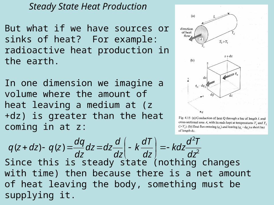
Steady State Heat Production

But what if we have sources or sinks of heat? For example: radioactive heat production in the earth.

In one dimension we imagine a volume where the amount of heat leaving a medium at (z +dz) is greater than the heat coming in at z:

2

2

)()(dz

Tdkdz

dz

dTk

dz

ddzdz

dz

dqzqdzzq

Since this is steady state (nothing changes with time) then because there is a net amount of heat leaving the body, something must be supplying it.

For radioactivity, it is useful to define A as the heat production rate per unit mass

2

2

dz

TdkdzAdz

Adz

Tdk

2

2

0

The total heat production in our volume then would be

dt

dQ

dVdt

dQ

dmA

11

or

dzAdVAdxdydt

dQ

dxdydz

dz

dq 11

and so

The biggest contribution to heat flow from radioactive decay in the Earth comes from U, Th, and K in the continental crust.

It also appears that the concentration of these elements in the crust decays exponentially with depth, and so the heat production must as well. We can therefore adopt:

DzoeAA /

Where D is a characteristic “skin depth”.

If we substitute this into the above equation and apply boundary conditions: To = surface temperature, qo = heat flow at surface and qm = heat flow from deep mantle, then the above diff. eq. will give:

DzoeA

kdz

Td /2

2

omo DAqq

1/ CeA

k

D

dz

dT Dzo

moz

o qDAdz

dTkq

0

1kCdz

dTkq

zm

Integrating:

Applying the heat flow boundary conditions:

Note that the minus sign is not used because the heat flow is in the –z direction. Thus

k

qeA

k

D

dz

dT mDzo /

2/

2

Czk

qeA

k

DT mDz

o

2

2

0CA

k

DTT ooz

oo A

k

DTC

2

2

Thus

Integrating again:

And applying the temperature b.c. at z = 0:

Or, since

)1( /2

Dzoo

m eAk

DTz

k

qT

Thus

omo DAqq

Dzmomo e

k

Dqq

k

zqTT /1)(

The equationomo DAqq

suggests that there should be a linear relation between the heat flow measured at the surface and the radioactive heat production rate measured at the surface, and this turns out to be the case. Generally, we find that D is about 10 km.

Non steady state heat conduction:

There are of course many situations where heat conduction is not constant in time. Your coffee gets cold, your beer warms up.

Generally, if you don’t supply heat to a conducting system, then the system will eventually become all the same temperature.

For now, let’s ignore volumetric heat production (A = 0). In fact, for a lot of common situations where we worry about bodies heating up or cooling off this is a good assumption.

The cooling/heating rate is just the rate of change of temperature = dT/dt.

Imagine a slab of width dz that is cooling; it will experience a net reduction in heat, which means that the heat flowing out is less than the heat flowing in.

We already described this situation above and found

2

2

)()(dz

Tdkdzzqdzzq

This change in heat flux results in a net change in the internal heat Q. Recall from above that a change in temperature is related to a change in heat by the specific heat cp , which has units J kg-1 K-1. If a unit volume

of the slab is dV, the change in heat per unit time is

The net heat flux is just this quantity divided by A. Thus

or

2

2

dz

Td

dt

dT

where = k/cp is called the thermal diffusivity. The above equation is

called the thermal diffusion equation or sometimes just the equation of heat conduction (something of a misnomer).

2

2

dz

Tddzk

dt

dTcdzdq p

dt

dTcAdz

dt

dQp

The general solution to the thermal diffusion equation is not trivial and often has to be figured out numerically, but there are a number of geologically significant situations where we can manipulate this equation into something easy to solve.

Case 1: Using separation of variables.

A useful technique for solving the diffusion equation is by separation of variables:

T(z,t) = (t)Z(z)

Substitution gives:

2

2 )()()()(

dz

zZtd

dt

zZtd

2

2 )()(

)()(

dz

zZdt

dt

tdzZ

2

2 )(

)(

1)(

)(

1

dz

zZd

zZdt

td

t

The left side depends only on time, the right side only on space. Thus, for example, if we specify a certain (t) then we can solve for Z(z) and vise versa.

A class of problems where this works very well is cyclical heating and cooling at the Earth’s surface, caused by daily, seasonal, or geologic (i.e., glacial) cycles.We can specify variations in the temperature at the surface of the Earth by

T(0, t) Toeit

where is the radial frequency = 2f, and we take the real part of this expression (the cosine). Try

Z(z) Aemz

and solve for A and m.Substitute:

e itie it i 1

Aemzm2Aemz m2

from which

m i

i

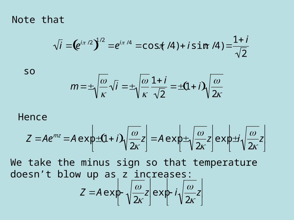
Note that

i e i / 2 1/ 2e i / 4 cos( /4) isin /4)

1 i

2

so

m

i

1 i

21 i

2

Hence

Z Aemz Aexp 1 i 2

z

Aexp

2

z

exp i

2

z

We take the minus sign so that temperature doesn’t blow up as z increases:

Z Aexp 2

z

exp i

2

z

)()(),( zZttzT

Where we recognize that T at z = 0 is To, so A = 1.

So then

ztizTo

2exp

2exp

This gives us a temperature distribution that decreases exponentially with depth and has a depth dependant phase shift. Both the rate of decay and the phase shift depend on the frequency.

zizAtiTo

2exp

2exp)exp(

Case 2: Instantaneous cooling of a semi infinite half space.

We need to solve this problem to understand how the lithosphere evolves. The solution can also be used to figure out how magma solidifies (or even how a lake freezes).

Here’s how we do it:

First, the BC’s of this problem are

T = Tm at t = 0, z > 0

T = Ts at z = 0, t > 0

T → Tm as z → ∞, t > 0

Define a dimensionless temperature as

T Tm

Ts Tm

and a dimensionless variable

z

2 t

Then we can rewrite the thermal diffusion equation as

dd

1

2

d2d2

or in other words, we convert a PDE of two variables (z, t) into an ODE of one variable (). This is much easier to deal with.

The solution to this ODE is

12

e '2

d'0

1 erf () erfc()

we call the integral part the “error function” and 1 minus that the “complimentary error function”. Resubstituting:

T Tm

Ts Tm

erfcz

2 t

or

t

zerf

t

zerfc

TT

TT

TT

TTTT

TT

TT

sm

s

ms

mms

ms

m

2211

T(z, t) Ts Tm Ts erfz

2 t

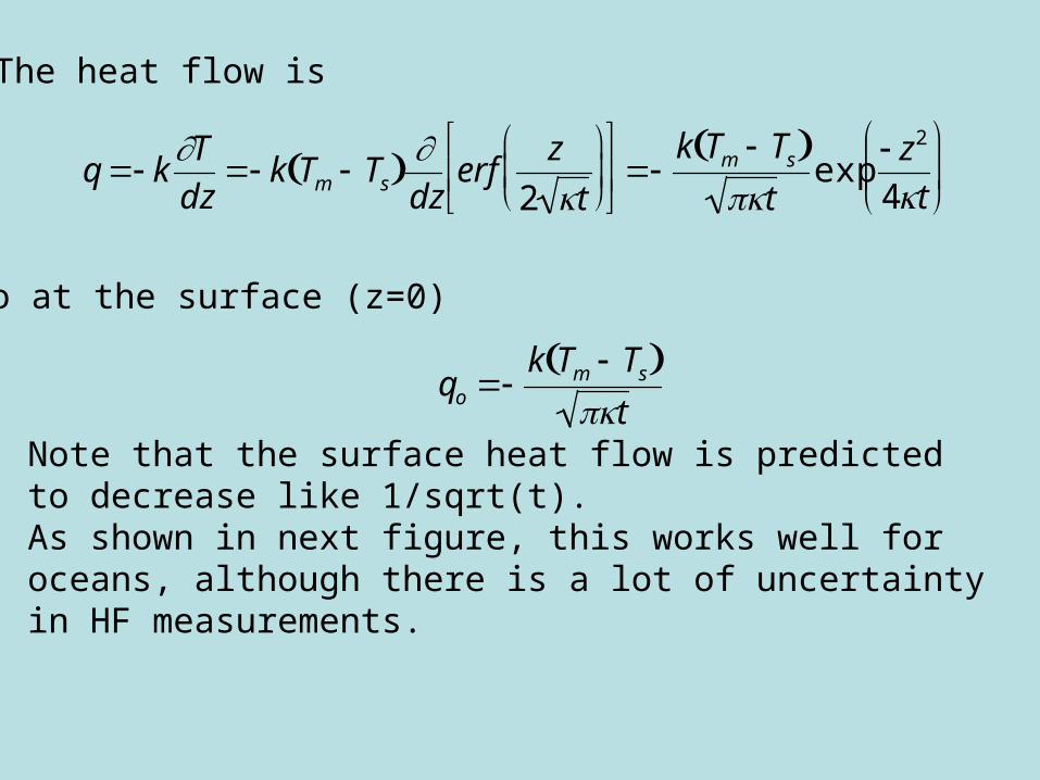
The heat flow is

q kT

dz k Tm Ts

dzerf

z

2 t

k Tm Ts t

exp z2

4t

so at the surface (z=0)

qo k Tm Ts

t

Note that the surface heat flow is predicted to decrease like 1/sqrt(t).As shown in next figure, this works well for oceans, although there is a lot of uncertainty in HF measurements.

We can also calculate what the depth of the oceans should by invoking isostacy. We consider that oceanic lithosphere is represented by some depth of water w above a cooling half space. Isostacy requires:

m w zL ww '(z')dz'0

zL

or

w m w '(z')dz'0

zL

mzL '(z') m dz'0

zL

but

'(z') m m Tm T(z') where is our thermal expansion coefficient. We can also extend let zL →∞ so that

w m w m Tm T(z') dz'0

m Tm T(z') dz'0

We know from the half space cooling solution that

T Tm

Ts Tm

erfcz

2 t

so

w m w m Tm T(z') dz'0

m Tm Ts erfcz'

2 t

dz'

0

or

w m w m Tm Ts t

tTTw

wm

smm

or in other words w should increase like sqrt(t). As shown in the following figure, this works ok for t < about 80 Million yrs, but then w flattens out.

One way to correct is to use the “plate model” instead of the “half space model”. The plate model specifies that the temperature at a certain depth should stay at Tm. Thus, at very old age, the heat flux is constant and T(z) is linear. This seems to fit the data pretty well for zL of about 125 km depth.

The source of the extra heat is presumed to be basal shear heating (from the lithosphere moving on top of the asthenosphere).

The descending slab

The slab heats back up as it descends into the mantle. Two complications:

1. Shear heating at the top: q = ut.

2. Phase changes. Olivine- spinel is exothermic; spinel-perovskite is endothermic.

To understand the effect, we need to know the P-T relationship at which the two phases can coexist. This relationship is called the Clapeyron curve.

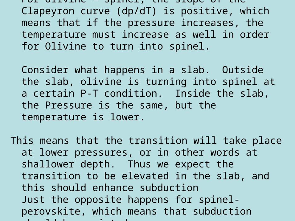
For Olivine – spinel, the slope of the Clapeyron curve (dp/dT) is positive, which means that if the pressure increases, the temperature must increase as well in order for Olivine to turn into spinel.

Consider what happens in a slab. Outside the slab, olivine is turning into spinel at a certain P-T condition. Inside the slab, the Pressure is the same, but the temperature is lower.

This means that the transition will take place at lower pressures, or in other words at shallower depth. Thus we expect the transition to be elevated in the slab, and this should enhance subductionJust the opposite happens for spinel-perovskite, which means that subduction should be resisted.

Convection

Conduction is the predominant mechanism for heat transfer near the surface, but it cannot be for the mantle. This is because the Earth is loosing too much heat. Near surface temperature gradients are on the order of 30K km-1, so that this rate the center of the Earth would be 200,000 K, and more importantly everything below a couple hundred km would be molten, and we know from seismology that the mantle is solid. To explain what happens in the mantle, we appeal to convection.

Recall that as you heat up something, it will expand, and hence become less dense. Thus, if you heat up something from the bottom, there will be a tendency to produce a gravitational instability.First, let’s recall what an adiabat is. It is the condition of no change in entropy, which means that the temperature of a body changes without any gain or loss of heat.

Imagine a small volume at a certain depth (= pressure) in equilibrium with its surroundings. Now, displace it to a shallower depth (less pressure). Remember that

PV ~ T

so if V is constant and there is no Q, then a decrease in P leads to a decrease in T. If that T just happens to be the same temperature as it’s new surroundings, there will be no Q (no temperature gradient) and no V. In other words, it is stable.

The temperature gradient that corresponds to this condition is called the adiabatic temperature gradient.

Now suppose the gradient is greater than adiabatic (superadiabatic). Then, as the volume ascends, it will still be hotter than its surroundings.

This will result in a volume increase, and hence a local density decrease, which creates a net gravitational buoyancy.

The opposite will occur if a downward displacement occurs (there will be a negative buoyancy produced).

BUT there is resistance to this process from

(1) viscosity of the surrounding medium and

(2) the conduction of heat away from the volume that will equilibrate it with its surroundings.

To figure out if the material will rise spontaneously or not (i.e., “convect”) we form a ratio between the forces that make it go up (buoyancy) and those keeping it down (conduction and viscosity) and we call this the Rayleigh number.

A useful form of the Rayleigh number is:

Ra = (g) D4

whereg gravitational acceleration thermal expansion coefficient superadiabatic temperature gradient (the gradient of the temperature above the adiabat) diffusivity dynamic viscosity (= regular viscosity/density)D thickness of the fluid layer

Note sensitivity of Ra to D!

Note that convective systems tend to be stabilizing: because heat is taken out of a system so efficiently, the temperature gradient tends to return to an adiabat.

Thus, the temperature gradient in a convecting system tends to be just slightly above adiabatic.

And of course we can make lab measurements on likely rocks and minerals to determine their thermal properties.

Even so, we have only a vague idea of how temperature changes with depth.

However, it seems clear that if the Earth’s interior cannot be loosing heat by conduction or radiation, it must be doing so by convection, and from what we learned before it seems most likely that the temperature gradient in the Earth is close to adiabatic.

So it is of interest to compute the adiabatic temperature gradient.

What can we say about temperature in the Earth?

Recall from seismology we know Vp and Vs, from which we can get , from which we can get pressure, and we also know about phase changes in from olivine-spinel and spinel-perovskite and the depth of the CMB.

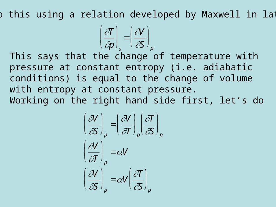
We can do this using a relation developed by Maxwell in late 1800s:

T

p

s

V

S

p

This says that the change of temperature with pressure at constant entropy (i.e. adiabatic conditions) is equal to the change of volume with entropy at constant pressure.Working on the right hand side first, let’s do

V

S

p

V

T

p

T

S

p

V

T

p

V

V

S

p

VT

S

p

Recall from 2nd law of thermo:

S Q

T

and that the relation between dQ and dT is

Q c pmT

So

T

S

T

Q /TT

T

Q

T

c pmHence

V

S

p

VT

S

p

VT

c pmT

c pand

T

p

s

T

c p

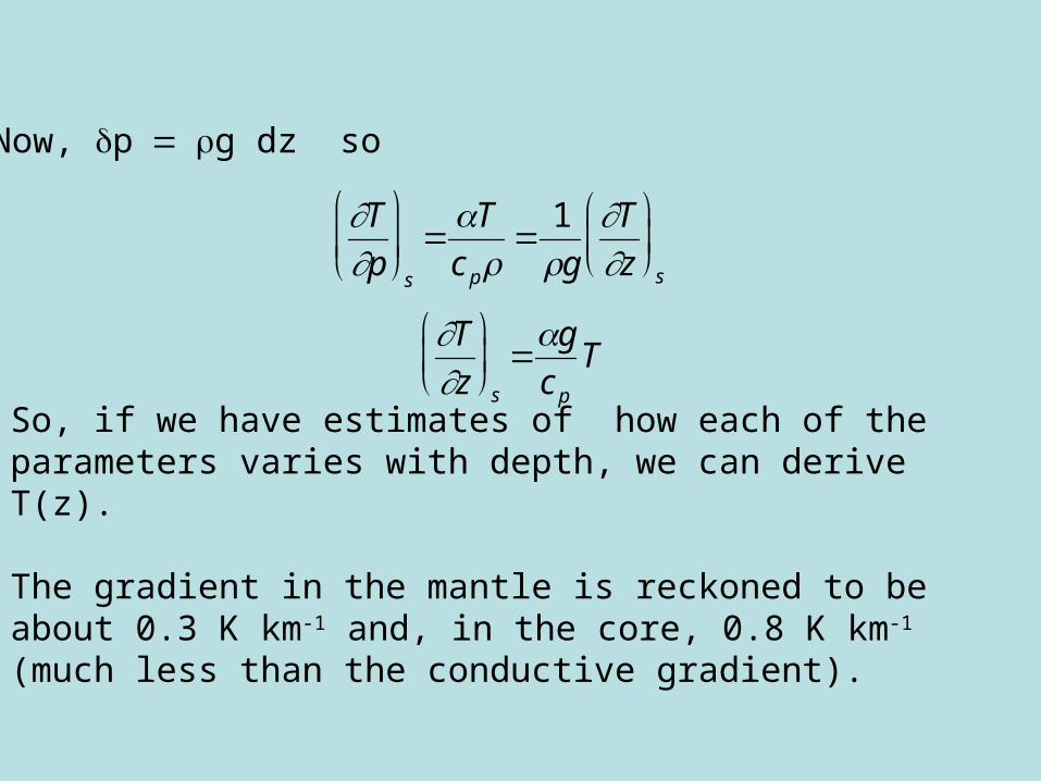
Now, pg dz so

T

p

s

T

c p

1

g

T

z

s

T

z

s

g

c p

T

So, if we have estimates of how each of the parameters varies with depth, we can derive T(z).

The gradient in the mantle is reckoned to be about 0.3 K km-1 and, in the core, 0.8 K km-1 (much less than the conductive gradient).