GEOTECHNICAL ENGINEERING – I (Subject Code: 06CV54) UNIT 4: FLOW …€¦ · modeling is governed...
26
Author: K.V. Vijayendra Department of Civil Engineering, BIT, Bangalore. 1 GEOTECHNICAL ENGINEERING – I (Subject Code: 06CV54) UNIT 4: FLOW OF WATER THROUGH SOILS Contents: Darcy’s law- assumption and validity, coefficient of permeability and its determination (laboratory and field), factors affecting permeability, permeability of stratified soils, Seepage velocity, Superficial velocity and coefficient of percolation, effective stress concept-total pressure and effective stress, quick sand phenomena, Capillary Phenomena. 4.1 Introduction: Water strongly affects engineering behaviour of most kind of soils and water is an important factor in most geotechnical engineering problems. Hence it is essential to understand basic principles of flow of water through soil medium. Flow of water take place through interconnected pores between soil particles is considered in one direction. Objectives of this chapter are to understand basic principles of one dimensional flow through soil media. This understanding has application in the problems involving seepage flow through soil media and around impermeable boundaries which are frequently encountered in the design of engineering structures. To understand the concepts involved in this particular subject, student is advised to review basic terminologies of fluid mechanics course [06 CV 35 – Fluid Mechanics]. This is essential because, as water flows through soil medium from a higher energy to a lower energy the concerned modeling is governed by the principles of fluid mechanics. 4.2 Permeability Flow of water in soil media takes place through void spaces which are apparently interconnected. Water can flow through the densest of natural soils. Water does not flow in a straight line but in a winding path (tortuous path) as shown in Figure 4.1. However, in soil mechanics, flow is considered to be along a straight line at an effective velocity. The velocity of drop of water at any point along its flow path depends on the size of the pore and its position inside the pore. Figure 4.1: Water flows in a winding path through soil media
Transcript of GEOTECHNICAL ENGINEERING – I (Subject Code: 06CV54) UNIT 4: FLOW …€¦ · modeling is governed...

Author: K.V. Vijayendra
Department of Civil Engineering, BIT, Bangalore.
1
GEOTECHNICAL ENGINEERING – I (Subject Code: 06CV54)
UNIT 4: FLOW OF WATER THROUGH SOILS Contents:
Darcy’s law- assumption and validity, coefficient of permeability and its determination
(laboratory and field), factors affecting permeability, permeability of stratified soils,
Seepage velocity, Superficial velocity and coefficient of percolation, effective stress
concept-total pressure and effective stress, quick sand phenomena, Capillary Phenomena.
4.1 Introduction:
Water strongly affects engineering behaviour of most kind of soils and water is an
important factor in most geotechnical engineering problems. Hence it is essential to
understand basic principles of flow of water through soil medium. Flow of water take
place through interconnected pores between soil particles is considered in one direction.
Objectives of this chapter are to understand basic principles of one dimensional flow
through soil media. This understanding has application in the problems involving seepage
flow through soil media and around impermeable boundaries which are frequently
encountered in the design of engineering structures. To understand the concepts involved
in this particular subject, student is advised to review basic terminologies of fluid
mechanics course [06 CV 35 – Fluid Mechanics]. This is essential because, as water
flows through soil medium from a higher energy to a lower energy the concerned
modeling is governed by the principles of fluid mechanics.
4.2 Permeability
Flow of water in soil media takes place through void spaces which are apparently
interconnected. Water can flow through the densest of natural soils. Water does not flow
in a straight line but in a winding path (tortuous path) as shown in Figure 4.1. However,
in soil mechanics, flow is considered to be along a straight line at an effective velocity.
The velocity of drop of water at any point along its flow path depends on the size of the
pore and its position inside the pore.
Figure 4.1: Water flows in a winding path through soil media

Author: K.V. Vijayendra
Department of Civil Engineering, BIT, Bangalore.
2
Since water can flow through the pore spaces in the soil hence soil medium is considered
to be permeable. Thus, the property of a porous medium such as soil by virtue of which
water can flow through it is called its permeability. In other words, the ease with which
water can flow through a soil mass is termed as permeability.
4.3 Darcy’s law
In 1856, modern studies of groundwater began when French scientist and engineer,
H.P.G. Darcy (1803-1858) was commissioned to develop a water-purification system for
the city of Dijon, France. He constructed the first experimental apparatus to study the
flow characteristics of water through the soil medium. From his experiments, he derived
the equation that governs the laminar (non-turbulent) flow of fluids in homogeneous
porous media which became to be known as Darcy’s law.
Figure 4.2: Schematic diagram depicting Darcy’s experiment
The schematic diagram representing Darcy’s experiment is depicted in Figure 4.2. By
measuring the value of the rate of flow, Q for various values of the length of the sample,
L, and pressure of water at top and bottom the sample, h1 and h2, Darcy found that Q is
proportional to (h1 – h2)/L or the hydraulic gradient, i, that is,
1 2h h hQ k A k A
L L
Q kiA
− ∆= =
=
The loss of head of ∆h units is affected as the water flows from h1 to h2. The hydraulic
gradient defined as loss of head per unit length of flow may be expressed as,
hi
L
∆=
Author: K.V. Vijayendra
Department of Civil Engineering, BIT, Bangalore.
3
k is coefficient of permeability or hydraulic conductivity with units of velocity, such as
mm/sec or m/sec. Thus the theory of seepage flow in porous media is based on a
generalization of Darcy's Law which is stated as, “Velocity of flow in porous soil media
is proportional to the hydraulic gradient” where, flow is assumed to be laminar. That is,
v = k i
Where, k is coefficient of permeability, v is velocity of flow and i is the hydraulic
gradient. Typical values of coefficient of permeability for various soils are as follows,
________________________________________________________________________
Soil type Coefficient of permeability (mm/s)
Coarse 10 – 103
Fine gravel, coarse, and medium sand 10−2
– 10
Fine sand, loose silt 10−4
– 10−2
Dense silt, clayey silt 10−5
– 10−4
Silty clay, clay 10−8
– 10−5
Assumptions made defining Darcy’ law.
� The flow is laminar that is, flow of fluids is described as laminar if a fluid
particles flow follows a definite path and does not cross the path of other
particles.
� Water & soil are incompressible that is, continuity equation is assumed to be valid
� The soil is saturated
� The flow is steady state that is, flow condition do not change with time.
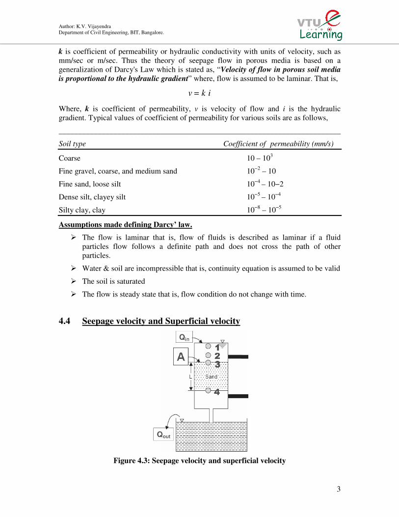
4.4 Seepage velocity and Superficial velocity
Figure 4.3: Seepage velocity and superficial velocity
Author: K.V. Vijayendra
Department of Civil Engineering, BIT, Bangalore.
4
Consider flow of water through soil medium of length L and cross sectional area A as
shown in Figure 4.3. If v is the velocity of downward movement of a drop of water from
positions 1 to 2 then velocity is equal to ki, therefore k can be interpreted as the ‘approach
velocity’ or ‘superficial velocity’ for unit hydraulic gradient, i.e.,.( 1)
vk k
i= =
=
Drop of water flows from positions 3 to 4 at faster rate than it does from positions 1 to 2
because the average area of flow channel through the soil is smaller. The actual velocity
of water flowing through the voids is termed as seepage velocity,s
v .
By the principle of continuity, the velocity of approach v, may be related to the seepage
velocity or average effective velocity of flow, vs by equating in
Q and out
Q as follows,
s v
s
v v v
s
Q vA v A
A AL Vv v v v
A A L V
v 1+e ki 1+ev = v = = ki
n e n e
= =
= = =
=
Where, Av = Area of pores, V = total volume of soil, Vv = volume of voids, e = voids ratio
and n = porosity. Thus seepage velocity is the superficial velocity divided by the
porosity. Above equation indicates that the seepage velocity is also proportional to the
hydraulic gradient.
s p
k (1+e)kv = i = i = k i,
n e
That is, ∝s pv k , where pk is called coefficient of percolation given by,
p
k (1+ e)kk = =
n e
Thus, coefficient of percolation is defined as the ratio of coefficient of permeability to
porosity.
4.5 Factors affecting permeability
The coefficient of permeability as used by geotechnical engineer is the approach or
superficial velocity of the permeant flowing through soil medium under unit hydraulic
gradient hence it depends on the characteristics of permeant, as well as those of the soil.
Considering the flow through a porous medium as similar to a flow through a bundle of
straight capillary tubes, the relationship showing the dependency of soil permeability on
various characteristic parameters of soil and permeant was developed by Taylor as given
below,

Author: K.V. Vijayendra
Department of Civil Engineering, BIT, Bangalore.
5
32 e
k = D C(1+e)
ρ
µ
This equation reflects the influence of permeant and the soil characteristics on
permeability. In the above equation D is the effective diameter of the soil particles, ρ is
the unit weight of fluid, µ is the viscosity of fluid and C is the shape factor. Therefore,
with the help of above equation, factors affecting permeability can be listed as follows,
Permeant fluid properties
i. Viscosity of the permeant
ii. Density and concentration of the permeant.
Soil characteristics
i. Grain-size
• Shape and size of the soil particles.
• Permeability varies with the square of particle diameter.
• Smaller the grain-size the smaller the voids and thus the lower the permeability.
• A relationship between permeability and grain-size is more appropriate in case
of sands and silts.
• Allen Hazen proposed the following empirical equation, 2
10k(cm / s) = C D ,
C is a constant that varies from 1.0 to 1.5 and D10 is the effective size, in mm
ii. Void ratio
• Increase in the porosity leads to an increase in the permeability.
• It causes an increase in the percentage of cross-sectional area available for flow.
iii. Composition
• The influence of soil composition on permeability is generally insignificant in
the case of gravels, sands, and silts, unless mica and organic matter are present.
• Soil composition has major influence in the case of clays.
• Permeability depends on the thickness of water held to the soil particles, which
is a function of the cation exchange capacity.
iv. Soil structural
• Fine-grained soils with a flocculated structure have a higher coefficient of
permeability than those with a dispersed structure.
• Remoulding of a natural soil reduces the permeability
• Permeability parallel to stratification is much more than that perpendicular to
stratification
v. Degree of saturation
• Higher the degree of saturation, higher is the permeability.
• In the case of certain sands the permeability may increase three-fold when the
degree of saturation increases from 80% to 100%.
vi. Presence of entrapped air and other foreign matter.
• Entrapped air reduces the permeability of a soil.
• Organic foreign matter may choke flow channels thus decreasing the
permeability
Author: K.V. Vijayendra
Department of Civil Engineering, BIT, Bangalore.
6
Hence, it is important to simulate field conditions in order make realistic estimate of the
permeability of a natural soil deposit, particularly when the aim is to determine field
permeability in the laboratory.
4.6 Validity or limitations of Darcy’s law
Darcy’s law given by v = k i is true for laminar flow through the void spaces. A criterion
for investigating the range can be furnished by the Reynolds number. For flow through
soils, Reynolds number Rn can be given by the relation,
n
vDR
g
ρ
µ=
Where, v=discharge (superficial) velocity in cm/s, D = average diameter of the soil
particle in cm, ρ= density of the fluid in g/cm3, µ= coefficient of viscosity in g/cm·s, g =
acceleration due to gravity, cm/s2
For laminar flow conditions in soils, experimental results show that,
1n
vDR
g
ρ
µ= ≤
with coarse sand, assuming D = 0.47 mm and k ≈ 100D2 = 100(0.047)2 = 0.2209 cm/s.
Assuming i = 1, then v = ki = 0.2209 cm/s.
Also, water ≈ 1g/cm3, and (µ at 20
0C) g = 10−5 (980) g/cm·s. Gives, 1≈nR = 1.059
From the above calculations, we can conclude that, for flow of water through all types of
soil (sand, silt, and clay), the flow is laminar and Darcy’s law is valid. With coarse sands,
gravels, and boulders, turbulent flow of water can be expected
4.7 Measurement of coefficient of permeability – Laboratory tests
There are two types of tests available for determining coefficient permeability in the
laboratory, namely,
i. Constant-head permeability test - suitable for coarse grained soils,
ii. Falling or Variable -head permeability test - suitable for fine grained soils,
Constant-head permeability test
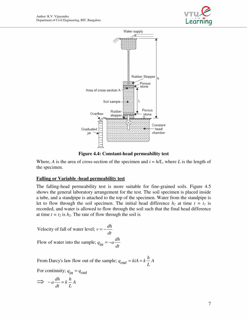
The constant-head test is suitable for more permeable coarse grained soils. The basic
laboratory test arrangement is shown in Figure 4.4. The soil specimen is placed inside a
cylindrical mold, and the constant-head loss h of water flowing through the soil is
maintained by adjusting the supply. The outflow water is collected in a measuring
cylinder, and the duration of the collection period is noted. From Darcy’s law, the total
quantity of flow Q in time t can be given by
Q qt kiAt= =
Q Lk
At h∴ =
Author: K.V. Vijayendra
Department of Civil Engineering, BIT, Bangalore.
7
Figure 4.4: Constant-head permeability test
Where, A is the area of cross-section of the specimen and i = h/L, where L is the length of
the specimen.
Falling or Variable -head permeability test
The falling-head permeability test is more suitable for fine-grained soils. Figure 4.5
shows the general laboratory arrangement for the test. The soil specimen is placed inside
a tube, and a standpipe is attached to the top of the specimen. Water from the standpipe is
let to flow through the soil specimen. The initial head difference h1 at time t = t1 is
recorded, and water is allowed to flow through the soil such that the final head difference
at time t = t2 is h2. The rate of flow through the soil is
Velocity of fall of water level;
Flow of water into the sample;
dhv
dt
dhq ain dt
= −
= −
From Darcy's law flow out of the sample;
For continuity;
hq kiA k Aout L
q qoutin
dh ha k A
dt L
= =
=
− =⇒

Author: K.V. Vijayendra
Department of Civil Engineering, BIT, Bangalore.
8
Figure 4.5: Falling or Variable -head permeability test
( )
1 1
2 2
1
1 22
Seperating the variables and integrating over the limits,
;
ln ( )
dh Ah ta k dt
h th L
h Aa k t t
h L
⇒ =∫ ∫
⇒ = −
( )
( )
1
2
1
2
ln
where - , interms of (log )1 2 10
2.303 log10
haLk
hAt
t t t
haLk
hAt
⇒ =
=
⇒ =
Thus measuring h1 and h2 during time t, k can be computed.
1 2 2 3 2 1 3Note: For constant t, at two instances, let water level fall from and , then, h to h h to h h h h=
4.8 Measurement of coefficient of permeability – Field tests
The coefficient of permeability of the permeable layer can be determined by pumping
from a well at a constant rate and observing the steady-state water table in nearby
observation wells. The steady-state is established when the water levels in the test well
and the observation wells become constant. When water is pumped out from the well, the
aquifer gets depleted of water, and the water table is lowered resulting in a circular
depression in the phreatic surface. This is referred to as the ‘Drawdown curve’ or ‘Cone
of depression’. The analysis of flow towards such a well was given by Dupuit (1863).
Author: K.V. Vijayendra
Department of Civil Engineering, BIT, Bangalore.
9
Assumptions
1. The aquifer is homogeneous.
2. Darcy’s law is valid.
3. The flow is horizontal.
4. The well penetrates the entire thickness of the aquifer.
5. Natural groundwater regime remains constant with time.
6. Dupuit’s theory is valid that is, i = dz/dr
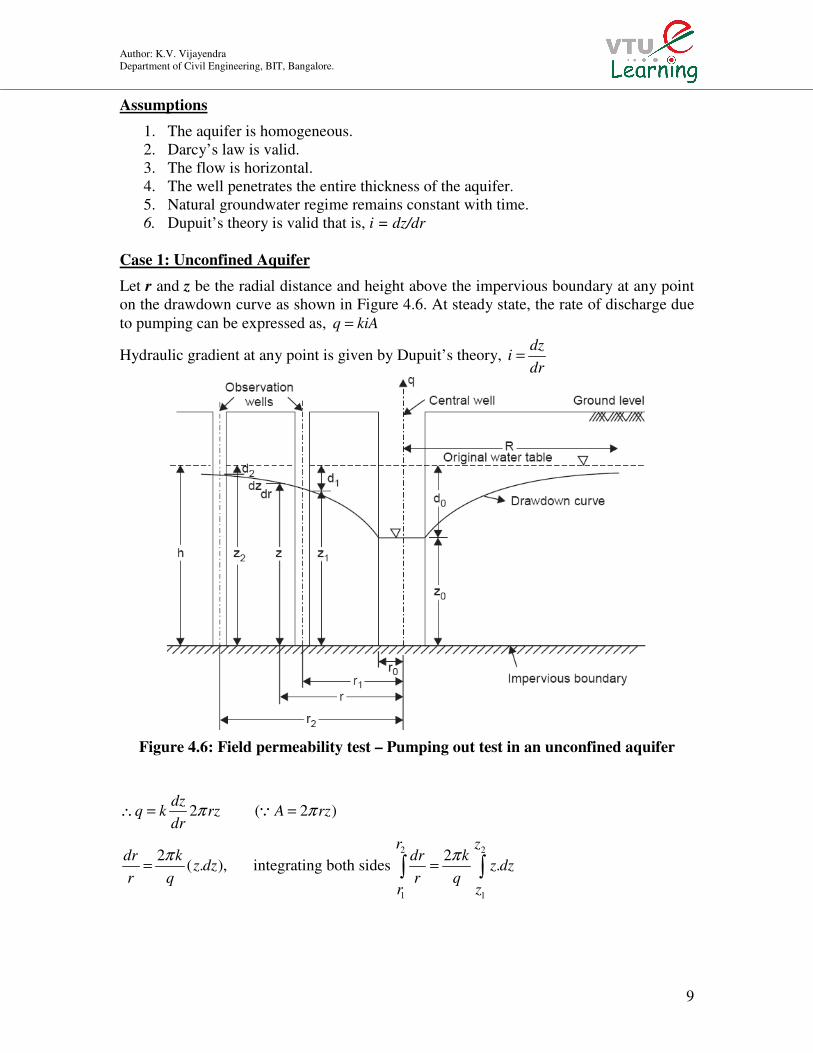
Case 1: Unconfined Aquifer
Let r and z be the radial distance and height above the impervious boundary at any point
on the drawdown curve as shown in Figure 4.6. At steady state, the rate of discharge due
to pumping can be expressed as, q kiA=
Hydraulic gradient at any point is given by Dupuit’s theory, dz
idr
=
Figure 4.6: Field permeability test – Pumping out test in an unconfined aquifer
2 2
1 1
2 ( 2 )
2 2( . ), integrating both sides .
dzq k rz A rz
dr
r zdr k dr k
z dz z dzr q r q
r z
π π
π π
∴ = =
= =∫ ∫
Q

Author: K.V. Vijayendra
Department of Civil Engineering, BIT, Bangalore.
10
2
2 2
2 1 1
2.303log
10( )
rqk
z z rπ
⇒ =
−
Note: z1 = (h – d1) & z2= (h – d2)
2
11 2 1 2
2.303log
10[( )(2 )]
q rk
rd d h d dπ
∴ =
− − −
If the values of r1, r2, z1, z2, and q are known from field measurements, the coefficient of
permeability can be calculated using the above relationship for k.
Case 2: Confined Aquifer
Let r and z be the radial distance and height above the impervious boundary at any point
on the drawdown curve as shown in Figure 4.7. At steady state, the rate of discharge due
to pumping can be expressed as, q kiA=
Figure 4.7: Field permeability test – Pumping out test in confined aquifer
2 2
1 1
2 ( 2 )
is depth of confined aquifer
integrating both sides, 2 2
dzq k rH A rH
dr
H
z rq dr q dr
kdz k dzH r H r
z r
π π
π π
∴ = =
= =∫ ∫
Q
22
11
[ ] log2
rqzk z rez H rπ
⇒ =

Author: K.V. Vijayendra
Department of Civil Engineering, BIT, Bangalore.
11
( ) ( )2 2
1 12 1 2 1
2.303log ; log10 102 ( ) 2.7283 ( )
r rq qk k
r rH z z H z zπ⇒ = ⇒ =
− × −
Note: z1 = (h – d1) & z2= (h – d2)
( )2
11 1
log102.7283 ( )
rqk
rH d d∴ =
× −
If the values of r1, r2, z1, z2, and q are known from field measurements, the coefficient of
permeability can be calculated using the above relationship for k.
4.9 Permeability of stratified soils
Case 1: Flow perpendicular to the layers.
Figure 4.7: Effective Permeability of stratified soils - perpendicular to the layers.
If , , ,1 2 1
are head lost in each of the corresponding layers
Then the total head lost is given by,
1 2 1
H H H H Hni n
H
H H H H H Hni n
∆ ∆ •••∆ •••∆ ∆−
∆
∆ = ∆ + ∆ + ••• + ∆ ••• +∆ + ∆−

Author: K.V. Vijayendra
Department of Civil Engineering, BIT, Bangalore.
12
Hydraulic gradients in each of these layers are,
11 2, , , ,1 2 1
1 2 1
Since discharge is same in all the layers, the velocity is the same in all layers
ie., 1 2
HH H H Hi n ni i i i ini nH H H H Hni n
q
v v
∆∆ ∆ ∆ ∆−= = ••• = ••• = =−
−
= =1
Let be the average permeability perpendicular (vertical) to the bedding planes
then, 11 2 2 1 1
v v vni n
kv
v k i k i k i k i k i k iv n ni i n n
••• = = ••• = =−
= = = = ••• = = ••• = =− −
ie.,
11 21 2 1
1 2 1
11 2, , , , , ,1 2 1
1 2 1
Substituting in the equation, 1 2 1
HH H H HH i n nv k k k k k kv ni nH H H H H Hni n
vHvH vH vH vHvH i n nH H H H H Hni nk k k k k kv ni n
H H H H H Hni n
vH
k
∆∆ ∆ ∆ ∆∆ −= = = = ••• = = •• = =−
−
−∴∆ = ∆ = ∆ = ••• ∆ = •• ∆ = ∆ =−
−
∆ = ∆ + ∆ + ••• + ∆ + •• +∆ + ∆−
⇒ 11 2
1 2 1
Effective permeability for flow in the direction perpendicular to layers is,
vHvH vH vH vHi n n
k k k k kv ni n
−= + + ••• + + ••• + +
−
∴
HHHH⇒ k =⇒ k =⇒ k =⇒ k =vvvv H HH HH HH HH HH HH HH H HHHH1 2 i n-1 n1 2 i n-1 n1 2 i n-1 n1 2 i n-1 n+ +•••+ +•••+ ++ +•••+ +•••+ ++ +•••+ +•••+ ++ +•••+ +•••+ +k k k k kk k k k kk k k k kk k k k knnnn1 n-11 n-11 n-11 n-12 i2 i2 i2 i
Case 2: Flow parallel to the layers.
Figure 4.8: Effective Permeability of stratified soils – parallel to the layers

Author: K.V. Vijayendra
Department of Civil Engineering, BIT, Bangalore.
13
If , , ,1 2 1
are rate of flow in each of the corresponding layers
Then the total rate of flow is given by,
1 2 1
Hydraulic gradients in each of these layers are same.
1
q q q q qni n
q
q q q q q qni n
i
••• •••−
= + + ••• + ••• + +−
=2 1
Since discharge, 1 2 1
i i i i ini n
q q q q q qni n
= ••• = ••• = = =−
= + + ••• + ••• + +−
ie., 1 1 2 2 1 1
Let be the average permeability parallel (Horizontal)
to the bedding planes then, Note that for flow in the horizontal direction
(which is the direct
q k iH k iH k iH k iH k iHn ni i n n
kh
= + + ••• + + ••• + +− −
ion of stratification of the soil layers),
the hydraulic gradient is the same for all layers.
1 1 2 2 1 1k iH k iH k iH k iH k iH k iHn ni i n nh
= + + ••• + + ••• + +− −
k H +k H +•••+k H +•••+k H +k Hk H +k H +•••+k H +•••+k H +k Hk H +k H +•••+k H +•••+k H +k Hk H +k H +•••+k H +•••+k H +k Hn nn nn nn n1 1 n-1 n-11 1 n-1 n-11 1 n-1 n-11 1 n-1 n-12 2 i i2 2 i i2 2 i i2 2 i i∴ k =∴ k =∴ k =∴ k =hhhh HHHH
kv and kh are effective are equivalent permeability coefficients for flow in parallel and
perpendicular directions to the bedding Planes respectively [Note: kv< kh].
4.10 Total Stress, Effective Stress and Pore Pressure
• External loading increases the total stress at every point in a saturated soil above
its initial value.
• The magnitude of this increase depends mostly on the location of the point
• The pressure transmitted through grain to grain at the contact points through a soil
mass is termed as inter-granular or effective pressure.
• It is known as effective pressure since this pressure is responsible for the decrease
in the void ratio or increase in the frictional resistance of a soil mass.
• If the pores of a soil mass are filled with water and if a pressure induced into the
pore water, tries to separate the grains, this pressure is termed as pore water
pressure or neutral stress. It is the same in all directions
The total stress, either due to self-weight of the soil or due to external applied forces or
due to both, at any point inside a soil mass is resisted by the soil grains as also by water
present in the pores or void spaces in the case of a saturated soil.
Total stress = Effective stress + Pore water Pressure (Neutral stress) ''''σ = σ + uσ = σ + uσ = σ + uσ = σ + u
Author: K.V. Vijayendra
Department of Civil Engineering, BIT, Bangalore.
14
( )
'
' '
If and are soil bulk unit weight and unit weight of water respectively, then at any depth, ,
Effective, total and neutral stresses relationship may be expressed as
b w
b w
b w
z
u z z
z z
γ γ
σ σ γ γ
σ γ γ γ
= − = −
= − =
where, w
u zγ= .
Usually the unit weight of soil varies with depth. Soil becomes denser with depth owing
to the compression caused by the geostatic stresses. If the unit weight of soil varies
continuously with depth, the vertical stress at any point, σv can be evaluated by means of
the integral:
0
.
z
vdzσ γ= ∫
If the soil is stratified, with different unit weights for each stratum, σv may be computed
conveniently by summation:
1
.( )n
v i
i
zσ γ=
= ∆∑
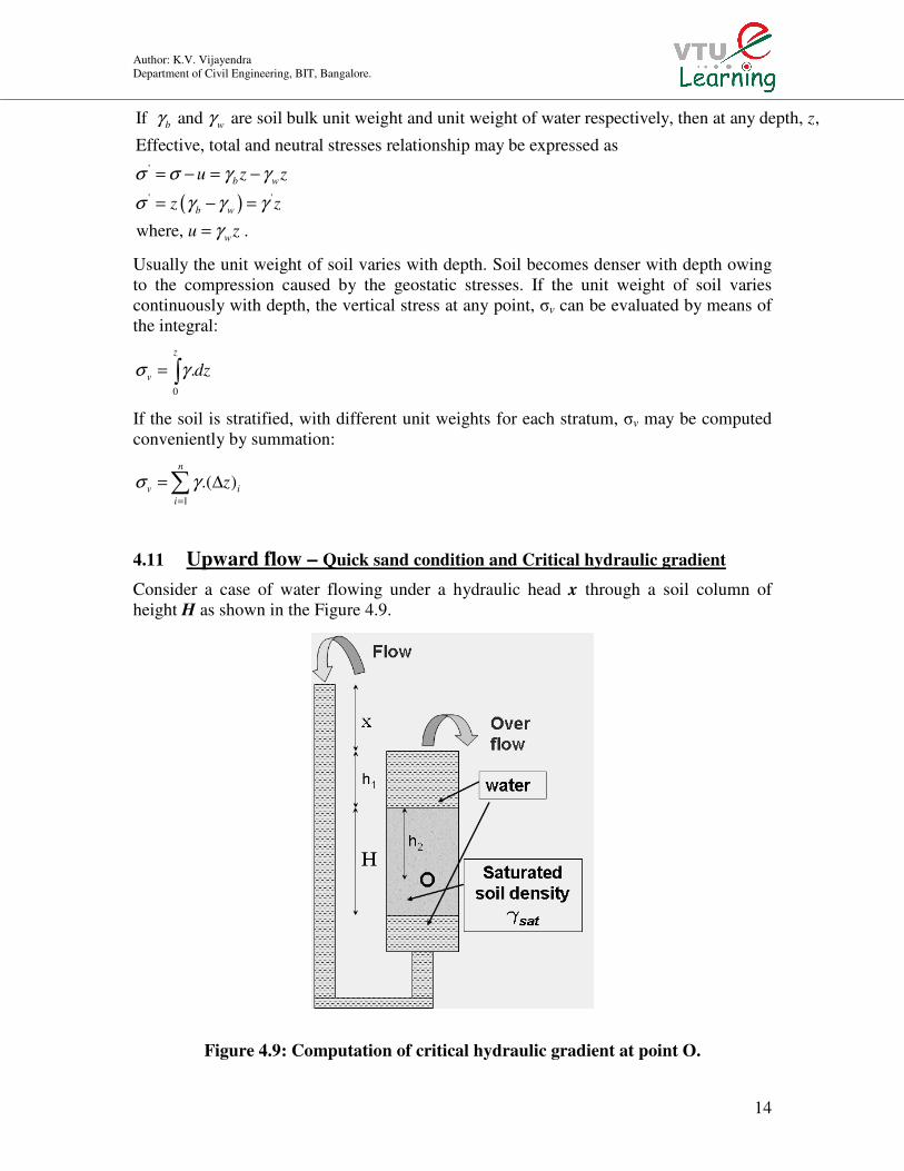
4.11 Upward flow – Quick sand condition and Critical hydraulic gradient
Consider a case of water flowing under a hydraulic head x through a soil column of
height H as shown in the Figure 4.9.
Figure 4.9: Computation of critical hydraulic gradient at point O.
Author: K.V. Vijayendra
Department of Civil Engineering, BIT, Bangalore.
15
The state of stress at point O situated at a depth of h2 from the top of soil column may be
computed as follows,
1 2
1 2
Vertical stress at O is,
If is the unit weight of water then pore pressure at O is,
( )
Ov w sat
w O
o w
h h
u
u h h x
σ γ γ
γ
γ
= +
= + +
'If and saturated and submerged unit weights of the soil column respectively,
Then effective stress at O is,
satγ γ
'
1 2 1 2
' '
2 2
'
' '
2
( ) ( )
( )
For quick sand condition(sand boiling) the effective stress tends to zero;
that is, 0
We get critical hydraulic gradient as,
Ov o w sat w
sat w w w
critical
w
u h h h h x
h x h x
i
h x
σ σ γ γ γ
σ γ γ γ γ γ
σ
σ γ γ
= − = + − + +
= − − = −
=
= − = 0;
'
2
( 1) 1 1
1 1
wcritical
w w
Gx Gi
h e e
γγ
γ γ
− −= = = × =
+ +
Where G is the specific gravity of the soil particles and e is the void ratio of the soil mass.
Therefore critical hydraulic gradient corresponds to hydraulic gradient which tends to a
state of zero effective stress. Hence critical hydraulic gradient is given by
1
1critical
Gi
e
−=
+
4.12 Capillary water in soil
• Capillary rise results from the combined actions of surface tension and inter-
molecular forces between the liquid and solids.
• The rise of water in soils above the ground water table is analogous to the rise of
water into capillary tubes placed in a source of water.
• But, the void spaces in a soil are irregular in shape and size, as they interconnect
in all directions.
• The pressure on the water table level is zero, any water above this level must have
a negative pressure.
• In soils a negative pore pressure increases the effective stresses and varies with
the degree of saturation
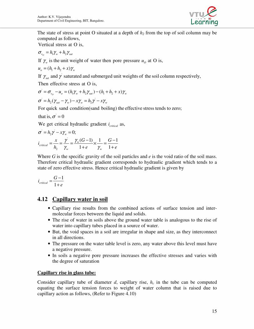
Capillary rise in glass tube:
Consider capillary tube of diameter d, capillary rise, hc in the tube can be computed
equating the surface tension forces to weight of water column that is raised due to
capillary action as follows, (Refer to Figure 4.10)
Author: K.V. Vijayendra
Department of Civil Engineering, BIT, Bangalore.
16
2
( ) cos4
4 cos 4; For pure water and a glass tube of very small diameter, 0,
s c w
s sc c
w w
dd T h
T Th h
d d
ππ α γ
αα
γ γ
× = ×
= = ∴ =
Figure 4.10: Capillary rise due to surface tension
4The maximum negative pore pressure is: s
c w
Tu h
dγ= =
The surface tension, TS for water at 20° C is equal to 75 x 10-8
kN/cm.
• The capillary process starts as water evaporates from the surface of the soil.
• The capillary zone is comprised of a fully saturated layer with a height of usually less
than hc, and a partially saturated layer overlain by wet or dry soil.
• Negative pore pressure results in an increase in the effective stress and is termed soil
suction.
• In granular materials (gravels and sands) the amount of capillary rise is negligible
while in fine grained soils the water may rise up to several meters.
EXAMPLE: 4.1
The results of a constant head permeability test on fine sand are as follows: area of the
soil specimen 180 cm2, length of specimen 320 mm, constant head maintained 460 mm,
and flow of water through the specimen 200mL in 5 min. Determine the coefficient of
permeability.
Data: L = 320 mm = 32 cm, Q = 200 ml.=200 cm3, A =180 cm
2, t = 5 minutes = 300 s
h = 460 mm = 46 cm
200 320.00258 /
180 300 46
0.0258 /
cm s
mm s
∴ = =×
∴
Q Lk =
At h
k =

Author: K.V. Vijayendra
Department of Civil Engineering, BIT, Bangalore.
17
EXAMPLE: 4.2
The discharge of water collected from a constant head permeameter in a period of 15
minutes is 400 ml. The internal diameter of the permeameter is 6 cm and the measured
difference in heads between the two gauging points 15 cm apart is 40. Calculate the
coefficient of permeability. If the dry weight of the 15 cm long sample is 7.0 N and the
specific gravity of the solids is 2.65, calculate the seepage velocity.
Data – I: Data – II: L = 15 cm G = 2.65
A = πD2/4 = π(36)/4=28.27 cm
2 L=15 cm
h = 40 cm Wdry = 7.0 N
Q = 400 ml.=400 cm3
t = 15 minutes = 900 s
400 150.0059 /
28.27 900 40cm s∴ = =
×
Q Lk =
At h
3
3
28.27 15 424.05
71000 16.51
424.05
2.65 9.81; 1 1.575; 0.575
1 16.51
0.5750.365; Superficial velocity,
1 1.575
0.00590
28.27 900
dry
w wdry
dry
Volume of the sample is
AL cm
kNDry density
m
G Ge e
e
en
e
Qv
At
γ
γ γγ
γ
= = × =
= × =
×= ∴ + = = = ∴ =
+
= = =+
= = =×
.016 /
0.016, 0.0438 /
0.365s
cm s
vseepage velocity v cm s
n∴ = = =
EXAMPLE: 4.3
In a falling head test permeability test initial head of 1.0 m dropped to 0.35 m in 3 hours,
the diameter being 5mm. The soil specimen is 200 mm long and 100 mm in diameter.
Calculate coefficient of permeability of the soil.
Data:
L = 200 mm
A =πD2/4 = π(100
2)/ 4 = 7853.98 mm
2; a =πD
2/4 = π(5
2)/ 4 = 19.635 mm
2
t = 3 hours=180 minutes = 10800 s
h1 = 1 m = 1000 mm, h2 = 0.35 m = 350 mm
110
2
510
2.303 log
100019.635 2002.303 log 4.86 10
3507853.98 10800
haLk
hAt
k mm−
=
×= = × ×
Author: K.V. Vijayendra
Department of Civil Engineering, BIT, Bangalore.
18
EXAMPLE: 4.4
A falling head permeability test is to be performed on a soil sample whose permeability is
estimated to be about 3 × 10⁻⁵
cm/s. What diameter of the standpipe should be used if the
head is to drop from 27.5 cm to 20.0 cm in 5 minutes and if the cross-sectional area and
length of the sample are respectively 15 cm2 and 8.5 cm ? Will it take the same time for
the head to drop from 37.7 cm to 30.0 cm ?
Data – I: L = 8.5 cm A = 15 cm2;
t = 5 minutes = 300 s h1 = 27.5 cm, h2 = 20.0 cm
Data – II: h1 = 37.7 cm, h2 = 30.0 cm
1 2
110 105
2
Time required for 37.7 to 30.0
37.70.049864 8.52.303 log ; 2.303 log
3015 3 10
215.22 300
h cm h cm
haLt t
hAk
t s t s it requires less time
−
= =
×= ⇒ = × × = < = ∴
EXAMPLE: 4.5
A sand deposit of 12 m thick overlies a clay layer. The water table is 3 m below the
ground surface. In a field permeability pump-out test, the water is pumped out at a rate of
540 liters per minute when steady state conditions are reached. Two observation wells are
located at 18 m and 36 m from the centre of the test well. The depths of the drawdown
curve are 1.8 m and 1.5 m respectively for these two wells. Determine the coefficient of
permeability.
Data:
r1 = 18 m, r2 = 36 m
h = 12 – 3 = 9.0 m
d1 = 1.8 m, d2 = 1.5 m
⇒ z1 = 9.0 – 1.8 = 7.2 m & z2 = 9.0 – 1.5 = 7.5 m
q = 540 lit / min = 540 /(60×1000) = 0.009 m3/s
(Refer to Figure E-4.5)
210 102 2
12 1
42 2
2.303 2.303 0.009 36log log 4.504 10 /18( ) (7.5 7.2 )
q rk m s
rz zπ π
−
×= = = ×
− −
52
10
3 10 15 3000.049864 ;
27.52.303 8.5 log
20
4 0.04986410 2.52
a cm
d mmπ
−× × ×∴ = =
× ×
×⇒ = × =
1 510 10
2
27.58.52.303 log ; 3 10 2.303 log
2015 300
haL ak
hAt
− ×= ⇒ × = ×

Author: K.V. Vijayendra
Department of Civil Engineering, BIT, Bangalore.
19
Figure E-4.5
EXAMPLE: 4.6
A pumping test carried out in a 50 m thick confined aquifer results in a flow rate of 600
lit/min. Drawdown in two observation wells located 50 m and 100 an from the well are 3
and 1 m respectively. Calculate the coefficient of permeability of the aquifer
Data:
r1 = 50 m, r2 = 100 m
H = 50 m
d1 = 3.0 m, d2 = 1.0 m
⇒ z1
= 70.0 – 3.0 = 67.0 m & z2 = 70.0 – 1.0 = 69.0 m
q = 600 lit / min = 600 /(60×1000) = 0.010 m3/s
(Refer to Figure E-4.6)
Figure E-4.6
210 10
12 1
5
1000.01log log
502.7283 ( ) 2.7283 50(69 67)
1.1034 10 /
rqk
rH z z
k m s−
= = × − × − = ×
Author: K.V. Vijayendra
Department of Civil Engineering, BIT, Bangalore.
20
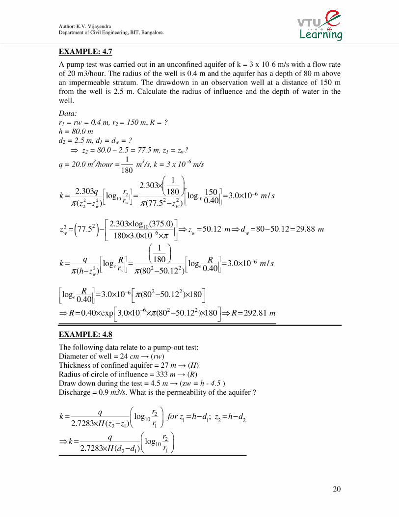
EXAMPLE: 4.7
A pump test was carried out in an unconfined aquifer of k = 3 x 10⁻⁶ m/s with a flow rate
of 20 m3/hour. The radius of the well is 0.4 m and the aquifer has a depth of 80 m above
an impermeable stratum. The drawdown in an observation well at a distance of 150 m
from the well is 2.5 m. Calculate the radius of influence and the depth of water in the
well.
Data:
r1 = rw = 0.4 m, r2 = 150 m, R = ?
h = 80.0 m
d2 = 2.5 m, d1 = dw = ?
⇒ z2 = 80.0 – 2.5 = 77.5 m, z1 = zw?
q = 20.0 m3/hour =
1
180 m
3/s, k = 3 x 10
-6 m/s
2
62 2
2 26
6 2 2
1
180log log 3.0 10 /0.40( ) (80 50.12 )
log 3.0 10 (80 50.12 ) 1800.40
0.40 exp 3.0 10 (80 50.12 ) 180 292.81
e ew
w
e
q R Rk m srh z
R
R R m
π π
π
π
−
−
−
= = = ×
− −
= × − ×
⇒ = × × × − × ⇒ =
EXAMPLE: 4.8
The following data relate to a pump-out test:
Diameter of well = 24 cm → (rw)
Thickness of confined aquifer = 27 m → (H)
Radius of circle of influence = 333 m → (R)
Draw down during the test = 4.5 m → (zw = h - 4.5 )
Discharge = 0.9 m3/s. What is the permeability of the aquifer ?
210 1 1 2 2
12 1
210
12 1
log ;2.7283 ( )
log2.7283 ( )
rqk for z h d z h d
rH z z
rqk
rH d d
= = − = − × −
⇒ = × −
( )
210 102 2
2
62 2
2 1026
12.303
2.303 180 150log log 3.0 10 /0.40( ) (77.5 )
2.303 log (375.0)77.5 50.12 80 50.12 29.88
180 3.0 10
ww w
w w w
q rk m s
rz z z
z z m d m
π π
π
−
−
× = = = ×
− −
× = − ⇒ = ⇒ = − = × × ×

Author: K.V. Vijayendra
Department of Civil Engineering, BIT, Bangalore.
21
10 10
3
3330.9log log
0.122.7283 ( 0) 2.7283 27 (4.5 0)
9.35 10 /
ww
Rqk
rH d
k m s−
= = × − × × − = ×
EXAMPLE: 4.9
A soil profile consists of three layers with the properties shown in the table below.
Calculate the equivalent coefficients of permeability parallel and normal to the stratum.
Layer Thickness (m) k (m/s)
1 3.0 2.0x 10 -6
2 4.0 5.0x 10
-8
3 3.0 3.0x 10 -5
Parallel to the layers.
-6 -8 -5-61 1 2 2 3 3
1 2 3
h
k H + k H + k H (2×10 ×3) + (5×10 × 4) + (3×10 ×3)= = 9.62×10 m / s
(H + H + H ) (3+ 4 + 3k =
)
Normal to the layers.
-7
v
31 2-6 -8 -5
1 2 3
H 10k = = = 1.23×10 m / s
3 4 3HH H+ ++ +
2×10 5×10 3×10k k k
EXAMPLE: 4.10
The data given below relate to two falling head permeameter tests performed on two
different soil samples:
(a) stand pipe area = 4 cm2, (b) sample area = 28 cm
2,
(c) sample height = 5 cm, (d) initial head in the stand pipe =100 cm,
(e) final head = 20 cm,
(f) time required for the fall of water level in test 1, t = 500 sec,
(g) for test 2, t = 15 sec.
Determine the values of k for each of the samples. If these two types of soils form
adjacent layers in a natural state with flow (a) in the horizontal direction, and (b) flow in
the vertical direction, determine the equivalent permeability for both the cases by
assuming that the thickness of each layer is equal to 150 cm.
1 310
2
1 310
2
1 :
2.303 4 5 1002.303 log log 2.3 10 /
28 500 20
2:
2.303 4 5 1002.303 log log 76.65 10 /
28 15 20
Test
haLk cm s
hAt
Test
haLk cm s
hAt
−
−
−
× ×⇒ = = = × ×
−
× ×⇒ = = = × ×

Author: K.V. Vijayendra
Department of Civil Engineering, BIT, Bangalore.
22
Horizontal direction flow
-3 -3
1 1 2 2h
1 2
k H + k H (2.3×10 ×150) + (76.65×10 ×150)k = = = 0.0395 cm / s
(H + H ) (150 +150)
Vertical direction flow
-3
v
1 2-3 -3
1 2
H 300k = = = 4.466×10 cm / s
150 150H H++
2.3×10 5×10k k
EXAMPLE: 4.11
A layer of clay of 4 m thick is overlain by a sand layer of 5 m, the top of which is the
ground surface. The clay overlay an impermeable stratum. Initially the water table is at
the ground surface but it is lowered 4 meters by pumping. Calculate σ’v at the top and
base of the clay layer before and after pumping. For sand e = 0.45, G = 2.6, Sr (sand, after
pumping) = 50%. For clay e = 1.0, G = 2.7.
( ) 3
( 50%)
(1 ) 2.6 9.81 (1 0.08654)19.113 /
1 1 0.45
0.45 .500.08654
2.7
r
wb sand S
r
G wkN m
e
eSw
G
γγ
=
+ × × += = =
+ +
×= = =
( )
( )
3
3
( ) 9.81 (2.6 0.45)20.635 /
1 1 0.45
( ) 9.81 (2.7 1.0)18.15 /
1 (1 1)
wsat sand
wsat clay
G ekN m
e
G ekN m
e
γγ
γγ
+ × += = =
+ +
+ × += = =
+ +
At the top of the clay layer before pumping:
σv = 20.635×5.0 = 103.175 kPa,
u = 9.81×5.0 = 49.0 kPa,
σv’ = 103.175 - 49.0 = 54.175 kPa.
At the base of the clay layer before pumping:
σv = 103.175 + 18.15x4.0 = 175.775 kPa.
u = 9.81×9.0= 88.3 kPa,
σv’ = 175.775 - 88.3 = 87.475 kPa
At the top of the clay layer after pumping:
σv = 19.113×4.0+ 20.635×1.0 = 97.087 kPa,
u = 9.81×1.0 = 9.81 kPa,

Author: K.V. Vijayendra
Department of Civil Engineering, BIT, Bangalore.
23
σv’ = 97.087 - 9.81 = 87.277 kPa.
At the base of the clay layer after pumping:
σv = 97.087 + 18.15×4.0 = 169.687 kPa,
u = 9.81×5.0 = 49.05 kPa,
σv’ = 172.99 -49.05 = 120.637 kPa.
∆σv’ (at the top) = 87.277 – 54.175 = 33.102 kPa.
∆σv’ (at the base) = 120.637 – 87.475 = 33.162 kPa.
The increase in the effective vertical stress throughout the clay layer is uniform.
EXAMPLE: 4.12
A soil profile is shown in figure. Plot the distribution of total stress, pore pressure and
effective stress up to a depth of 12 m.
( ) ( )
( )( ) ( )
3
3
3
3
0.0 2.0
2.65 9.8016.23 /
1 1 0.6
2.0 5.0
(2.65 0.6) 9.8019.91 /
1 1 0.6
5.0 8.0
20.5 /
8.0 12.0
22.0 /
wdry
w
sat
sat
sat
m m
GkN m
e
m m
G ekN m
e
m m
kN m
m m
kN m
γγ
γγ
γ
γ
−
×= = =
+ +
−
+ + ×= = =
+ +
−
=
−
=

Author: K.V. Vijayendra
Department of Civil Engineering, BIT, Bangalore.
24
3
3
3 3
3
3
0.0 0.0, 0.0, 0.0
2.0 0.0, 16.23 2 32.46 / ,
32.46 0.0 32.46 /
5.0 3 9.8 29.4 / , 32.46 19.91 3 92.19 / ,
92.19 29.4 62.79 /
8.0 6 9.8 58.80 / , 92.19 20.50 3
z m u
z m u kN m
kN m
z m u kN m kN m
kN m
z m u kN m
σ σ
σ
σ
σ
σ
σ
′= ⇒ = = =
= ⇒ = = × =
′ = − =
= ⇒ = × = = + × =
′ = − =
= ⇒ = × = = + × = 3
3
3
3
3
153.69 / ,
153.69 58.80 94.89 /
12.0 10 9.8 98.0 / ,
153.69 22.0 4 241.69 / ,
241.69 98.0 143.69 /
kN m
kN m
z m u kN m
kN m
kN m
σ
σ
σ
′ = − =
= ⇒ = × =
= + × =
′ = − =
Depth (m) u = z γw (kPa) σ = z γsat (kPa) σ’= σ-u (kPa)
0.0 0.00 0.00 0.00
2.0 0.00 32.46 32.46
5.0 29.40 92.19 62.79
8.0 58.80 153.69 94.89
12.0 98.00 241.69 94.89
Figure: Example: 4.12 - Pore pressure, Total stress and Effective stress Distribution

Author: K.V. Vijayendra
Department of Civil Engineering, BIT, Bangalore.
25
EXAMPLE: 4.13
If a glass tube of 0.002 mm diameter is immersed in water, what is the height to which
water will rise in the tube by capillary action? Derive the necessary expression for
capillary rise and use the same.
TS = 75 x 10-8 kN/cm. = 75 x 10-6 kN/m.
D = 0.002 × 10⁻³
m
γw = 9.80 kN/m3
6
3
4 4 75 10
0.002 10 9.80
15.36
sc
w
c
Th
d
h m
γ
−
−
× ×= =
× ×
=
EXAMPLE: 4.14
What is the height of capillary rise in a soil with an effective size of 0.06 mm and void
ratio of 0.72 ?
3 3
3 5 3
1
5 3
6
3
0.05
(0.05)
0.72
0.72 (0.05) 9 10
, , (9 10 ) 0.0448
4 4 75 10Capillary rise, 0.683
0.0448 9.80 10
sc
w
Effective size mm
Volume of solids mm
voidratio
Volume of voids mm
Approximately void size d mm
Th m
dγ
−
−
−
−
=
=
=
= × = ×
= × =
× ×= = =
× ×
EXAMPLE: 4.15
Water is flowing at the rate of 50 mm3/s in an upward direction through a sample of sand
whose coefficient of permeability is 2x10 -2
mm/s. The sample thickness is 120 mm and
cross section area is 5000 mm2. Determine the effective pressure at the middle and at
bottom sections of the sample. Take the saturated unit weight of sand as 19 KN/m3.
( )
- 23 2
3
sat w
- 2
'
w
- 3'
'
z=120mm
q = 50 mm / s; k = 2×10 mm / s; A = 5000 mm ; z = 120 mm
γ' = γ - γ = 19.0 - 9.80 = 9.2 kN / m
q 50Hydraulic gradient = i = = = 0.5
kA 2×10 ×5000
For upward flow, σ = z×(γ' - iγ )
At the bottom; z = 120 mm; σ = 120×10 ×(9.2 - 0.5×9.8)
σ = 0.516 k
⇒
⇒
( )
- 3'
'
z=60mm
Pa
At the middle; z = 60 mm; σ = 60×10 ×(9.2 - 0.5×9.8)
σ = 0.258 kPa
⇒

Author: K.V. Vijayendra
Department of Civil Engineering, BIT, Bangalore.
26
EXAMPLE: 4.16
A 1.60 m layer of the soil of specific gravity, G = 2.66 and porosity, n= 38% is subject to
an upward seepage head of 2.0 m. What depth of coarse sand would be required above
the soil to provide a factor of safety of 1.5 against quick sand condition assuming that the
coarse sand has the same porosity and specific gravity as the soil and that there is
negligible head loss in the sand?
0.382.66; 38% 0.613
1 1 0.38
1 2.66 1; 1.029
1 1 0.613
2, 2.916
0.686
1.60
c
nG n e
n
GCritical hydraulic gradient i
e
hLength of flow required is L m
i
Available thickness of soil m
Additional thickness of sand layer requir
= = ⇒ = = =− −
− −⇒ = = =
+ +
= = =
=
∴
2.916 1.60 1.316
1.316
ed
d m
Additional thickness of sand layer required m
= − =
=
************************************************
Reference:
1. V. N. S. Murthy, “Geotechnical Engineering: Principles and Practices of Soil
Mechanics and Foundation Engineering”, Marcel Dekker, Inc.,
2. Braja M. Das, “Advanced Soil Mechanics”, Third edition, Taylor & Francis
3. T.W. Lambe & R.V. Whitman, “Soil Mechanics”, John Wiley & Sons
4. B.C. Punmia, “Soil Mechanics and Foundations”, Laxmi Publications (P) Ltd.
5. C. Venkatramaiah, “Geotechnical Engineering”, Newage International (P)
Limited, Publishers, Third ed., 2006.
************************************************