
Geosynthetic Reinforced Soil Performance Testing— … · Geosynthetic Reinforced Soil Performance...
172
Geosynthetic Reinforced Soil Performance Testing— Axial Load Deformation Relationships PUBLICATION NO. FHWA-HRT-13-066 AUGUST 2013 Research, Development, and Technology Turner-Fairbank Highway Research Center 6300 Georgetown Pike McLean, VA 22101-2296
Transcript of Geosynthetic Reinforced Soil Performance Testing— … · Geosynthetic Reinforced Soil Performance...

Geosynthetic Reinforced Soil Performance Testing—Axial Load Deformation Relationships
PubLicATion no. FHWA-HRT-13-066 AuGuST 2013
Research, Development, and TechnologyTurner-Fairbank Highway Research Center6300 Georgetown PikeMcLean, VA 22101-2296

FOREWORD
The use of geosynthetic reinforced soil (GRS) for load bearing applications such as bridge
abutments and integrated bridge systems (IBS) has expanded among transportation agencies
looking to save time and money while delivering a better and safe product to the traveling public.
GRS has been identified by the Federal Highway Administration (FHWA) as a proven, market-
ready technology, and is being actively promoted through its Every Day Counts (EDC) initiative.
FHWA interim design guidance for GRS abutments and IBSs is presented in Publication No.
FHWA-HRT-11-026. The guidance includes the procedure and use of the GRS performance
tests, also termed a mini-pier experiment. This report presents a database of nineteen
performance tests performed by the FHWA, largely at the Turner-Fairbank Highway Research
Center. It also presents findings, conclusions, and suggestions regarding various design
parameters related to the performance of GRS, such as backfill material, reinforcement strength,
reinforcement spacing, facing confinement, secondary reinforcement, and compaction.
A reliability analysis for load and resistance factor design (LRFD) was performed based on the
results of this performance testing to determine a calibrated resistance factor for the soil-
geosynthetic capacity equation. The results of this analysis can also be used by bridge designers
to estimate capacity and deformation of GRS. In addition, an insight into the behavior of GRS as
a new composite material due to the close reinforcement spacing is described.
Jorge E. Pagán-Ortiz
Director, Office of Infrastructure
Research and Development
Notice
This document is disseminated under the sponsorship of the U.S. Department of Transportation
in the interest of information exchange. The U.S. Government assumes no liability for the use
of the information contained in this document. This report does not constitute a standard,
specification, or regulation.
The U.S. Government does not endorse products or manufacturers. Trademarks or
manufacturers’ names appear in this report only because they are considered essential to the
objective of the document.
Quality Assurance Statement The Federal Highway Administration (FHWA) provides high-quality information to serve
Government, industry, and the public in a manner that promotes public understanding. Standards
and policies are used to ensure and maximize the quality, objectivity, utility, and integrity of its
information. FHWA periodically reviews quality issues and adjusts its programs and processes to
ensure continuous quality improvement.

TECHNICAL REPORT DOCUMENTATION PAGE
1. Report No.
FHWA-HRT-13-066
2. Government Accession No.
3. Recipient’s Catalog No.
4. Title and Subtitle
Geosynthetic Reinforced Soil Performance Testing—Axial Load Deformation Relationships
5. Report Date
August 2013
6. Performing Organization Code:
HRDI-40
7. Author(s)
Nicks, J.E., Adams, M.T., Ooi, P.S.K., Stabile, T.
8. Performing Organization Report No.
9. Performing Organization Name and Address
Turner-Fairbank Highway Research Center
6300 Georgetown Pike
McLean, VA 22101
10. Work Unit No.
11. Contract or Grant No.
N/A
12. Sponsoring Agency Name and Address
Office of Infrastructure R&D
FHWA Research, Development and Technology
6300 Georgetown Pike McLean, VA 22101
13. Type of Report and Period Covered
Technical
14. Sponsoring Agency Code
15. Supplementary Notes
The FHWA Contracting Officer’s Technical Representative (COTR) was Mike Adams, HRDI-40.
16. Abstract
The geosynthetic reinforced soil (GRS) performance test (PT), also called a mini-pier experiment, consists of constructing alternating layers of compacted granular fill and geosynthetic reinforcement with a facing element
that is frictionally connected, then axially loading the GRS mass while measuring deformation to monitor
performance. This large element load test provides material strength properties of a particular GRS composite
built with unique combinations of reinforcement, compacted fill, and facing elements. This report describes the
procedure and provides axial load- deformation results for a series of PTs conducted in both Defiance County,
OH, as part of the Federal Highway Administration’s (FHWA) Every Day Counts (EDC) GRS Validation
Sessions and in McLean, VA, at the FHWA’s Turner-Fairbank Highway Research Center as part of a parametric
study.
The primary objectives of this research report are to: (1) build a database of GRS material properties that can be
used by designers for GRS abutments and integrated bridge systems; (2) evaluate the relationship between
reinforcement strength and spacing; (3) quantify the contribution of the frictionally connected facing elements at
the service limit and strength limit states; (4) assess the new internal stability design method proposed by Adams
et al. 2011 for GRS; and (5) perform a reliability analysis of the proposed soil-geosynthetic capacity equation for
LRFD calibration. (1,11)
17. Key Words
Geosynthetic reinforced soil, performance test, mini-pier
experiment, abutment, integrated bridge system, geotextile,
capacity, deformation
18. Distribution Statement
19. Security Classif. (of this report)
Unclassified
20. Security Classif. (of this page)
Unclassified
21. No. of Pages
169
22. Price
Form DOT F 1700.7 (8-72) Reproduction of completed page authorized

ii
SI* (MODERN METRIC) CONVERSION FACTORS APPROXIMATE CONVERSIONS TO SI UNITS
Symbol When You Know Multiply By To Find Symbol
LENGTH in inches 25.4 millimeters mm ft feet 0.305 meters m yd yards 0.914 meters m mi miles 1.61 kilometers km
AREA in
2square inches 645.2 square millimeters mm
2
ft2
square feet 0.093 square meters m2
yd2
square yard 0.836 square meters m2
ac acres 0.405 hectares ha mi
2square miles 2.59 square kilometers km
2
VOLUME fl oz fluid ounces 29.57 milliliters mL gal gallons 3.785 liters L ft
3 cubic feet 0.028 cubic meters m
3
yd3
cubic yards 0.765 cubic meters m3
NOTE: volumes greater than 1000 L shall be shown in m3
MASS oz ounces 28.35 grams glb pounds 0.454 kilograms kgT short tons (2000 lb) 0.907 megagrams (or "metric ton") Mg (or "t")
TEMPERATURE (exact degrees) oF Fahrenheit 5 (F-32)/9 Celsius
oC
or (F-32)/1.8
ILLUMINATION fc foot-candles 10.76 lux lx fl foot-Lamberts 3.426 candela/m
2 cd/m
2
FORCE and PRESSURE or STRESS lbf poundforce 4.45 newtons N lbf/in
2poundforce per square inch 6.89 kilopascals kPa
APPROXIMATE CONVERSIONS FROM SI UNITS
Symbol When You Know Multiply By To Find Symbol
LENGTHmm millimeters 0.039 inches in m meters 3.28 feet ft m meters 1.09 yards yd km kilometers 0.621 miles mi
AREA mm
2 square millimeters 0.0016 square inches in
2
m2 square meters 10.764 square feet ft
2
m2 square meters 1.195 square yards yd
2
ha hectares 2.47 acres ac km
2 square kilometers 0.386 square miles mi
2
VOLUME mL milliliters 0.034 fluid ounces fl oz
L liters 0.264 gallons gal m
3 cubic meters 35.314 cubic feet ft
3
m3
cubic meters 1.307 cubic yards yd3
MASS g grams 0.035 ounces ozkg kilograms 2.202 pounds lbMg (or "t") megagrams (or "metric ton") 1.103 short tons (2000 lb) T
TEMPERATURE (exact degrees) oC Celsius 1.8C+32 Fahrenheit
oF
ILLUMINATION lx lux 0.0929 foot-candles fc cd/m
2candela/m
20.2919 foot-Lamberts fl
FORCE and PRESSURE or STRESS N newtons 0.225 poundforce lbf kPa kilopascals 0.145 poundforce per square inch lbf/in
2
*SI is the symbol for th International System of Units. Appropriate rounding should be made to comply with Section 4 of ASTM E380. e
(Revised March 2003)
iii
TABLE OF CONTENTS
1. INTRODUCTION ....................................................................................................................... 1 1.1 BACKGROUND .............................................................................................................. 1
1.2 CURRENT PERFORMANCE TESTS ........................................................................ 4 1.3 INTERNAL STABILITY DESIGN .............................................................................. 5 1.4 OBJECTIVES .................................................................................................................. 9
2. TESTING CONDITIONS ........................................................................................................ 11
2.1 BACKFILL CONDITIONS ......................................................................................... 11 2.1.1 Sieve Analysis..................................................................................................... 12 2.1.2 Density ................................................................................................................ 15
2.1.3 Friction Angle ..................................................................................................... 15
2.2 REINFORCEMENT CONDITIONS ......................................................................... 17 2.3 FACING CONDITIONS .............................................................................................. 17
3. TEST SETUP ............................................................................................................................. 19
3.1 LAYOUT ......................................................................................................................... 19 3.2 LOAD AND REACTION FRAME ............................................................................. 20 3.3 CONSTRUCTION ......................................................................................................... 25
3.4 INSTRUMENTATION ................................................................................................. 27 3.5 LOAD SCHEDULE AND COLLECTION OF DATA ............................................ 28
4. RESULTS DATABASE............................................................................................................ 29
4.1 UNLOAD/RELOAD BEHAVIOR .............................................................................. 33
4.2 REPEATABILITY ........................................................................................................ 38 4.3 COMPOSITE BEHAVIOR.......................................................................................... 38
5. COMPARISON TO PLANE STRAIN CONDITIONS ...................................................... 45
5.1 CAPACITY ..................................................................................................................... 45
5.2 STIFFNESS..................................................................................................................... 48
6. PARAMETRIC ANALYSIS.................................................................................................... 53
6.1 EFFECT OF AGGREGATE TYPE ........................................................................... 53 6.2 EFFECT OF COMPACTION ..................................................................................... 54
6.3 EFFECT OF BEARING BED REINFORCEMENT ............................................... 58 6.4 EFFECT OF GRADATION......................................................................................... 61 6.5 EFFECT OF REINFORCEMENT STRENGTH ..................................................... 64
6.6 EFFECT OF THE RELATIONSHIP BETWEEN REINFORCEMENT
STRENGTH AND SPACING ................................................................................................ 65 6.7 EFFECT OF FACING .................................................................................................. 71
7. APPLICATIONS OF PERFORMANCE TESTING TO DESIGN .................................. 79
7.1 DESIGN DATABASE ................................................................................................... 79 7.2 STRENGTH LIMIT ...................................................................................................... 80
7.2.1 Analytical ............................................................................................................ 80
7.2.2 Empirical ............................................................................................................. 84
7.3 SERVICE LIMIT........................................................................................................... 87

iv
7.4 LRFD CALIBRATION FOR STRENGTH LIMIT ................................................. 93 7.4.1 Background ......................................................................................................... 93
7.4.2 Reliability Analysis: FOSM ............................................................................... 94 7.4.3 Resistance Factor ................................................................................................ 97
8. CONCLUSIONS ........................................................................................................................ 99
APPENDIX A. SOIL TESTING DATA ....................................................................................103
APPENDIX B. NUCLEAR DENSITY TESTING FOR TFHRC PTS .................................115
APPENDIX C. DEFORMATION INSTRUMENTATION LAYOUTS FOR PTS ............125
APPENDIX D. RAW DATA FOR PTS .....................................................................................131
ACKNOWLEGEMENTS .............................................................................................................149
REFERENCES................................................................................................................................151
v
LIST OF FIGURES
Figure 1. Photo. Vegas mini-pier experiment ..................................................................................... 1 Figure 2. Illustration. Plan view of Vegas mini-pier experiment ...................................................... 2 Figure 3. Illustration. Face view of Vegas mini-pier experiment ...................................................... 2 Figure 4. Illustration. Side view of Vegas mini-pier experiment ...................................................... 3 Figure 5. Illustration. Reinforcement schedule for Vegas mini-pier experiment ............................. 4 Figure 6. Illustration. Plan view of Defiance County experiment ..................................................... 5 Figure 7. Illustration. Elevation view of Defiance County (DC) test ................................................ 5 Figure 8. Equation. Ultimate vertical capacity for a GRS composite ............................................... 6 Figure 9. Equation. W factor ................................................................................................................ 6 Figure 10. Equation. Required reinforcement strength ...................................................................... 6 Figure 11. Equation. Confining stress (Wu et al. 2010) ..................................................................... 7 Figure 12. Graph. Predictive capability of the soil-geosynthetic composite capacity equation ..... 8 Figure 13. Graph. Predictive capability of the required reinforcement strength equation ............... 8 Figure 14. Graph. Reinforced backfill gradations ............................................................................ 14 Figure 15. Graph. LSDS testing results ............................................................................................. 16 Figure 16. Photo. DC-1 GRS PT (before testing) ............................................................................. 20 Figure 17. Illustration. Concrete footing on GRS composite, inset from facing ............................ 21 Figure 18. Photo. Hollow core hydraulic jacks for PT assembly .................................................... 21 Figure 19. Photo. TF-1 PT setup with reaction frame ...................................................................... 22 Figure 20. Photo. TF-6 PT setup with reaction frame ...................................................................... 23 Figure 21. Photo. TF-10 PT setup with reaction frame .................................................................... 23 Figure 22. Photo. TF-9 at failure with reaction frame ...................................................................... 24 Figure 23. Photo. Spherical bearing to apply load to the footing on the GRS composite ............. 25 Figure 24. Illustration. Instrumentation layout for DC tests and TF-1............................................ 27 Figure 25. Illustration. General additional instrumentation layout TF PT series ........................... 28 Figure 26. Graph. Load-deformation behavior for the Defiance County PTs ................................ 30 Figure 27. Graph. Load-deformation behavior for the Turner Fairbank PTs ................................. 31 Figure 28. Photo. Tilting of the footing during TF-4 testing ........................................................... 32 Figure 29. Graph. TF-4 results ........................................................................................................... 33 Figure 30. Graph. TF-1 results ........................................................................................................... 35 Figure 31. Graph. TF-5 results ........................................................................................................... 36 Figure 32. Graph. TF-6 results ........................................................................................................... 37 Figure 33. Graph. Repeatability of PT at TFHRC. ........................................................................... 39 Figure 34. Photo. TF-11 at failure with Sv = 3-13/16 inches, Tf = 1,400 lb/ft, and 21A
material ............................................................................................................................. 40 Figure 35. Photo. TF-3 at failure with Sv = 7⅝ inches, Tf = 2,400 lb/ft, and 21A material .......... 40 Figure 36. Photo. TF-13 at failure with Sv = 11¼ inches, Tf = 3,600 lb/ft, and 21A material ...... 41 Figure 37. Photo. TF-10 at failure with Sv = 15¼ inches, Tf = 4,800 lb/ft, and 21A material. ..... 41 Figure 38. Photo. Rupture pattern for geotextiles in TF-6 (qult,emp = 43,828 psf); the lowest
layer of reinforcement is the closet fabric in the picture ............................................... 43 Figure 39. Photo. Post-test picture of TF-6 (Sv = 7⅝ inches, Tf = 4,800 lb/ft)............................... 44 Figure 40. Equation. Mohr-Coulomb shear strength ........................................................................ 45 Figure 41. Equation. Ultimate capacity of an unconfined GRS PT ................................................ 45 Figure 42. Equation. Ultimate capacity of a strip footing on slope ................................................. 45

vi
Figure 43. Equation. Ultimate capacity of a strip footing on a vertical GRS abutment................. 45 Figure 44. Equation. Ratio of plane strain capacity to PT capacity ................................................ 46 Figure 45. Equation. Stability Factor ................................................................................................ 46 Figure 46. Graph. Ratio of plane strain capacity to PT capacity for different stability factors .... 46 Figure 47. Graph. Mohr-Coulomb failure envelope for Pham (2009) plane strain GSGC tests .. 47 Figure 48. Graph. Plane strain capacity to PT capacity for a stability factor of 0.29 .................... 48 Figure 49. Illustration. Infinitely Long Unconfined GRS abutment ............................................... 48 Figure 50. Equation. Stiffness of an Infinitely Long Unconfined GRS abutment ......................... 49 Figure 51. Illustration. Solution for strip footing on top of a wall .................................................. 49 Figure 52. Equation. Vertical displacement of a GRS abutment with a strip footing .................... 50 Figure 53. Equation. Vertical strain................................................................................................... 50 Figure 54. Equation. Stiffness of a GRS abutment supporting a strip footing ............................... 50 Figure 55. Equation. Vertical displacement of a GRS abutment with a strip footing. ................... 50 Figure 56. Graph. Ratio of plane strain stiffness of a strip footing on top of a wall (SGRS) to
that of a PT (SPT) for the case of constant stiffness with depth..................................... 51
Figure 57. Graph. Comparison between compacted and uncompacted GRS composites ............. 56 Figure 58. Design service limit for uncompacted sample DC-5...................................................... 57 Figure 59. Graph. Comparison of compacted and uncompacted strains between the DC-1
and DC-5 tests .................................................................................................................. 58 Figure 60. Graph. Effect of bearing bed reinforcement for TF-7 and TF-8.................................... 59 Figure 61. Graph. Measured lateral deformation at 3,600 psf applied stress for TF-7 (no
bearing bed reinforcement) and TF-8 (2 courses of bearing bed reinforcement) ....... 60 Figure 62. Graph. Measured lateral deformation at 26,600 psf applied stress for TF-7 (no
bearing bed reinforcement) and TF-8 (2 courses of bearing bed reinforcement) ....... 61 Figure 63. Graph. Comparison of open-graded and well-graded backfills for TF-1 and TF-2 .... 63 Figure 64. Graph. Stress-strain curves for PTs with CMUs at Tf/Sv = 3,800 psf ........................... 67 Figure 65. Graph. Stress-strain curves for PTs with no CMU facing at Tf/Sv = 3,800 psf ............ 68 Figure 66. Graph. Capacity of GRS with no CMU facing at various reinforcement spacing
for different Tf/Sv ratios ................................................................................................... 69 Figure 67. Graph. Capacity of GRS with CMU facing at various reinforcement spacing for
different Tf/Sv Ratios ....................................................................................................... 70 Figure 68. Graph. Capacity of GRS with no CMU facing at various reinforcement strength
for different Tf/Sv ratios ................................................................................................... 70 Figure 69. Graph. Capacity of GRS with CMU facing at various reinforcement strength for
different Tf/Sv ratios ......................................................................................................... 71 Figure 70. Graph. Stress-strain response for TF-2 (CMU facing) and TF-3 (No CMU facing)
with Sv = 7⅝ inches and Tf = 2,400 lb/ft ........................................................................ 72 Figure 71. Stress-strain response for TF-6 (CMU facing) and TF-7 (No CMU facing) with
Sv = 7⅝ inches and Tf = 4,800 lb/ft ................................................................................. 72 Figure 72. Graph. Stress-strain response for TF-9 (CMU facing) and TF-10 (No CMU
facing) with Sv = 15¼ inches and Tf = 4,800 lb/ft ......................................................... 73 Figure 73. Graph. Stress-strain Response for TF-12 (CMU facing) and TF-11 (No CMU
facing) with Sv = 3-13/16 inches and Tf = 1,400 lb/ft .................................................... 74 Figure 74. Graph. Stress-strain response for TF-14 (CMU facing) and TF-13 (No CMU
facing) with Sv = 11¼ inches and Tf = 3,600 lb/ft ......................................................... 74

vii
Figure 75. Graph. Effect of CMU facing on ultimate capacity as a function of reinforcement
spacing .............................................................................................................................. 77 Figure 76. Graph. Effect of CMU facing on ultimate capacity as a function of reinforcement
strength ............................................................................................................................. 77 Figure 77. Graph. Calculated confining pressure due to CMU facing at the ultimate capacity ... 78 Figure 78. Graph. Comparison of predicted capacity and measured capacity................................ 80 Figure 79. Graph. Cumulative distribution function plot for DC and TF PTs................................ 81 Figure 80. Graph. Cumulative distribution function plot for all GRS composite tests .................. 83 Figure 81. Graph. Normalized applied stress versus strain for all PT ............................................. 85 Figure 82. Graph. Normalized load-deformation behavior for the DC and TF PTs up to
5 percent vertical strain.................................................................................................... 86 Figure 83. Graph. Cumulative distribution function for proposed service limit pressure ............. 88 Figure 84. Graph. Load-deformation behavior for the Turner Fairbank PTs at low strain
levels ................................................................................................................................. 90 Figure 85. Graph. Normalized load-deformation behavior for the DC and TF PTs up to
0.5 percent vertical strain ................................................................................................ 91 Figure 86. Graph. PTs strictly meeting FHWA GRS abutment design specifications................... 92 Figure 87. Equation. Limit state function for FOSM approach ....................................................... 94 Figure 88. Graph. Reliability index for lognormal R and Q ............................................................ 94 Figure 89. Equation. LRFD format ................................................................................................... 95 Figure 90. Equation. Resistance factor using FOSM ....................................................................... 95 Figure 91. Equation. Coefficient of variation for factored load ...................................................... 95 Figure 92. Equation. Coefficient of variation for resistance ............................................................ 96 Figure 93. Graph. Resistance factor for footings on GRS composites for different dead to
dead plus live load ratios and target reliability indices based on PT series ................. 97 Figure 94. Graph. Resistance factor for footings on GRS composites for different dead to
dead plus live load ratios and target reliability indices based on all testing to date .... 98 Figure 95. Graph. AASHTO No. 8 LSDS test results (DC tests) .................................................. 106 Figure 96. AASHTO No. 8 LSDS deformation test results (DC tests) ......................................... 107 Figure 97. Graph. AASHTO No. 8 pea gravel LSDS test results (DC tests) ............................... 108 Figure 98. Graph. AASHTO No. 8 pea gravel LSDS deformation test results (DC tests) .......... 108 Figure 99. Graph. AASHTO No. 57 LSDS test results (DC tests)................................................ 109 Figure 100. Graph. AASHTO No. 57 LSDS deformation test results (DC tests) ........................ 110 Figure 101. Graph. AASHTO No. 9 LSDS test results (DC tests)................................................ 111 Figure 102. Graph. AASHTO No. 9 LSDS deformation test results (DC tests) .......................... 111 Figure 103. Graph. AASHTO No. 8 LSDS test results (TFHRC tests) ........................................ 112 Figure 104. Graph. AASHTO No. 8 LSDS deformation test results (DC tests) .......................... 113 Figure 105. Graph. AASHTO A-1-a (VDOT 21A) LSDS test results (TFHRC tests) ................ 114 Figure 106. Graph. AASHTO A-1-a (VDOT 21A) LSDS deformation test results (DC tests) .. 114 Figure 107. Illustration. Instrumentation layout for DC tests and TF-1........................................ 125 Figure 108. Illustration. Instrumentation layout for TF-2, TF-9 ................................................... 125 Figure 109. Illustration. Instrumentation layout for TF-3, TF-4 ................................................... 126 Figure 110. Illustration. Instrumentation layout for TF-5, TF-7 ................................................... 126 Figure 111. Instrumentation layout for TF-6, TF-12 ...................................................................... 127 Figure 112. Illustration. Instrumentation layout for TF-8 .............................................................. 127 Figure 113. Illustration. Instrumentation layout for TF-10 ............................................................ 128

viii
Figure 114. Illustration. Instrumentation layout for TF-11 ............................................................ 128 Figure 115. Illustration. Instrumentation layout for TF-13 ............................................................ 129 Figure 116. Illustration. Instrumentation layout for TF-14 ............................................................ 129

ix
LIST OF TABLES
Table 1. Summary of PT conditions .................................................................................................. 11 Table 2. PT reinforced backfill gradations ........................................................................................ 12 Table 3. PT backfill gradation properties .......................................................................................... 13 Table 4. Maximum dry density for PT aggregates ........................................................................... 15 Table 5. LSDS testing results............................................................................................................. 16 Table 6. Geosynthetic reinforcement properties ............................................................................... 17 Table 7. PT dimensions ...................................................................................................................... 19 Table 8. PT measured results summary............................................................................................. 29 Table 9. Parametric study on aggregate size ..................................................................................... 53 Table 10. Effect of aggregate type results ......................................................................................... 54 Table 11. Parametric study on compaction ....................................................................................... 55 Table 12. Parametric study on bearing bed reinforcement .............................................................. 59 Table 13. Parametric study on gradation (Tf = 2,400 lb/ft, Sv = 7⅝ inches)................................... 62 Table 14. Parametric study on gradation (Tf = 4,800 lb/ft, Sv = 7⅝ inches)................................... 64 Table 15. Parametric study on reinforcement strength with open-graded aggregates ................... 64 Table 16. Parametric study on reinforcement strength with well-graded aggregates .................... 64 Table 17. Parametric study for 3,800 lb/ft
2 Tf/Sv ratio (with facing) .............................................. 65
Table 18. Parametric study for 3,800 lb/ft2 Tf/Sv ratio (with no facing) ......................................... 66
Table 19. Tf/Sv ratios for each PT ...................................................................................................... 66 Table 20. Effect of CMU facing on stiffness and capacity .............................................................. 75 Table 21. Effect of CMU facing on strain......................................................................................... 76 Table 22. PTs meeting GRS strength and service limit design criteria ........................................... 79 Table 23. Predicted and measured vertical capacity for DC and TF PTs ....................................... 82 Table 24. Predicted and measured vertical capacity for all GRS composite tests .......................... 83 Table 25. Estimation of allowable dead load to limit vertical strain to 0.5 percent using the
GRS capacity equation ...................................................................................................... 89 Table 26. Statistics for dead and live loads ....................................................................................... 96 Table 27. AASHTO No. 8 sieve analysis (DC tests) ..................................................................... 103 Table 28. AASHTO No. 8 pea gravel sieve analysis (DC tests) ................................................... 103 Table 29. AASHTO No. 57 Sieve analysis (DC tests) ................................................................... 104 Table 30. AASHTO No. 9 Sieve analysis (DC tests) ..................................................................... 104 Table 31. AASHTO No. 8 Sieve analysis (TFHRC tests) ............................................................. 105 Table 32. AASHTO A-1-a (VDOT 21A) sieve analysis (TFHRC tests) ...................................... 105 Table 33. Summary of AASHTO No. 8 LSDS results (DC tests) ................................................. 106 Table 34. Summary of AASHTO No. 8 pea gravel LSDS results (DC tests) .............................. 107 Table 35. Summary of AASHTO No. 57 LSDS results (DC tests)............................................... 109 Table 36. Summary of AASHTO No. 9 LSDS results (DC tests) ................................................. 110 Table 37. Summary of AASHTO No. 8 LSDS results (TFHRC tests) ......................................... 112 Table 38. Summary of AASHTO A-1-a (VDOT 21A) LSDS results (TFHRC tests) ................. 113 Table 39. TF-2 Nuclear density test results .................................................................................... 115 Table 40. TF-2 Nuclear density test results .................................................................................... 116 Table 41. TF-3 Nuclear density test results .................................................................................... 117 Table 42. TF-4 Nuclear density test results .................................................................................... 117 Table 43. TF-5 Nuclear density test results .................................................................................... 118

x
Table 44. TF-6 Nuclear density test results .................................................................................... 118 Table 45. TF-7 Nuclear density test results .................................................................................... 119 Table 46. TF-8 Nuclear density test results .................................................................................... 119 Table 47. TF-9 Nuclear density test results .................................................................................... 120 Table 48. TF-10 Nuclear density test results .................................................................................. 120 Table 49. TF-11 Nuclear density test results .................................................................................. 121 Table 50. TF-12 Nuclear density test results .................................................................................. 122 Table 51. TF-13 Nuclear density test results .................................................................................. 123 Table 52. TF-14 Nuclear density test results .................................................................................. 123 Table 53. DC-1 PT Data ................................................................................................................... 131 Table 54. DC-2 PT Data ................................................................................................................... 132 Table 55. DC-3 PT Data ................................................................................................................... 133 Table 56. DC-4 PT Data ................................................................................................................... 134 Table 57. DC-5 PT Data ................................................................................................................... 135 Table 58. TF-1 PT Data .................................................................................................................... 136 Table 59. TF-2 PT Data .................................................................................................................... 137 Table 60. TF-3 PT Data .................................................................................................................... 137 Table 61. TF-4 PT Data .................................................................................................................... 138 Table 62. TF-5 PT Data .................................................................................................................... 139 Table 63. TF-6 PT Data .................................................................................................................... 140 Table 64. TF-7 PT Data .................................................................................................................... 141 Table 65. TF-8 PT Data .................................................................................................................... 142 Table 66. TF-9 PT Data .................................................................................................................... 143 Table 67. TF-10 PT Data.................................................................................................................. 144 Table 68. TF-11 PT Data.................................................................................................................. 145 Table 69. TF-12 PT Data.................................................................................................................. 146 Table 70. TF-13 PT Data.................................................................................................................. 147 Table 71. TF-14 PT Data.................................................................................................................. 148

xi
LIST OF ABBREVIATIONS AND SYMBOLS
Abbreviations
AASHTO American Association of State Highway and Transportation Officials
CMU Concrete masonry unit
DC Defiance County, OH
EDC Every Day Counts initiative
FHWA Federal Highway Administration
GP-GM Poorly graded-silty gravel
GRS Geosynthetic reinforced soil
IBS Integrated bridge systems
LFD Load factor design
LRFD Load and resistance factor design
LSDS Large scale direct shear
LVDT Linear voltage displacement transducers
MARV Minimum average roll value
POT Potentiometer
PT Performance test
SRW Segmental retaining wall
TFHRC Turner-Fairbank Highway Research Center
USCS Unified Soil Classification System
Symbols
Reliability index
Slope angle
Target reliability index
β
βs
βT

xii
Unit weight of the backfill
γb Bulk unit weight of the facing block
Maximum dry density
Load factor for dead load
Load factor for live load
Unit weight of the GRS composite
Load factor for load component i
Interface friction angle between the geosynthetic and the facing element for a
frictionally connected GRS composite
Measured vertical strain at an applied load of 4000 psf
Measured vertical strain at failure
Maximum recorded vertical strain
Vertical strain
Vertical strain for a compacted GRS composite
Vertical strain for an uncompacted GRS composite
Bias, ratio of measured to predicted
Bias factor for dead load
Bias factor for live load
Bias factor for resistance
Poisson’s ratio of the GRS
Vertical displacement
Applied normal stress
External confining stress due to the facing
γ
γd
D
L
GRS
i
δ
ε@q=4000psf
ε@qult
εmax
v
εv,compact
εv,uncompact
λ
D
L
R
GRS
ρ
σc
xiii
Total lateral stress within the GRS composite at a given depth and location
Shear strength of soil
Peak friction angle
Friction angle of the GRS composite
Resistance factor
Φcap Resistance factor for capacity
Optimum moisture content
a Footing offset from the edge of the wall face (i.e., setback distance)
b Footing width on top of the GRS composite
B Base width of the GRS composite
Btotal Total width of the PT with the CMU facing
c Cohesion of the backfill
cGRS Cohesion of the GRS composite
Cc Coefficient of Curvature
Cu Coefficient of Uniformity
d Depth of the facing block unit perpendicular to the wall face
dmax Maximum aggregate size
D10 Aggregate size in which 10 percent of the sample is finer
D30 Aggregate size in which 30 percent of the sample is finer
D60 Aggregate size in which 60 percent of the sample is finer
D85 Aggregate size in which 85 percent of the sample is finer
Eo Initial stress-strain ratio
Eo,CMU Initial stress-strain ratio for tests with CMU facing
Eo, no CMU Initial stress-strain ratio for tests without any facing
σh
ϕ
GRS
Φ
ω

xiv
EGRS Young’s modulus of the GRS composite
ER Ratio of stress to strain for the reload cycle
ḡ Mean safety margin
H Height of the GRS composite
Kar Coefficient of active earth pressure for the backfill
Kpr Coefficient of passive earth pressure for the backfill
L Length of footing/bearing area
Bearing capacity factor
Ncq Bearing capacity factor
Ns Stability factor
SGRS Plane strain stiffness of a strip footing on top of GRS
SPT Stiffness of the unconfined GRS column
Sv Reinforcement spacing
Tf Wide width tensile strength of the geosynthetic, expressed as the minimum
average roll value (MARV)
Treq,c Required reinforcement strength in the direction perpendicular to the wall face
q Applied stress
Applied stress at 0.5 percent vertical strain
Predicted applied stress at 0.5 percent vertical strain
Applied stress at 5 percent vertical strain
qmax Maximum applied pressure during testing
qult,an,c Ultimate capacity using semi-empirical theory
qult,emp Measured failure pressure
qult,emp CMU Measured failure pressure for tests with CMU facing
qult,emp no CMU Measured failure pressure for tests without any facing
Nq
q@ε=0.5%
q@ε=0.5%, predicted
q@ε=5%
xv
qult,PS Ultimate capacity of strip footing under plane strain conditions
qult,PT Ultimate capacity of the GRS column
Q Load
QD Dead load
QL Live load
Qi Load component i
R Resistance
Vdmax Coefficient of variation of the maximum aggregate size
VD Coefficient of variation of the dead load
VKp Coefficient of variation of the coefficient for passive earth pressure
VL Coefficient of variation of the live load
VM Coefficient of variation of the model
VQ Coefficient of variation of the loads
VR Coefficient of variation of the resistance
VTf Coefficient of variation of the reinforcement strength
W Factor accounting for the effect of reinforcement spacing and aggregate size
z Standard normal variable

1
1. INTRODUCTION
The Federal Highway Administration (FHWA) has developed a standard test method to describe
the load-deformation behavior of a frictionally connected geosynthetic reinforced soil (GRS)
composite material which can be used to predict performance of a GRS abutment.(1)
The GRS
performance test (PT), also called a mini-pier experiment, consists of constructing alternating
layers of compacted granular fill and geosynthetic reinforcement with a facing element that is
frictionally connected, then axially loading the GRS mass while measuring deformation to
monitor performance. This large element load test provides material strength properties of a
particular GRS composite built with different combinations of reinforcement, compacted fill, and
facing elements. This report describes the procedure and provides axial load versus deformation
results for a series of PTs conducted in both Defiance County, OH, as part of the FHWA’s Every
Day Counts (EDC) GRS Validation Sessions and in McLean, VA, at the FHWA’s Turner-
Fairbank Highway Research Center (TFHRC) as part of a parametric study.
1.1 BACKGROUND
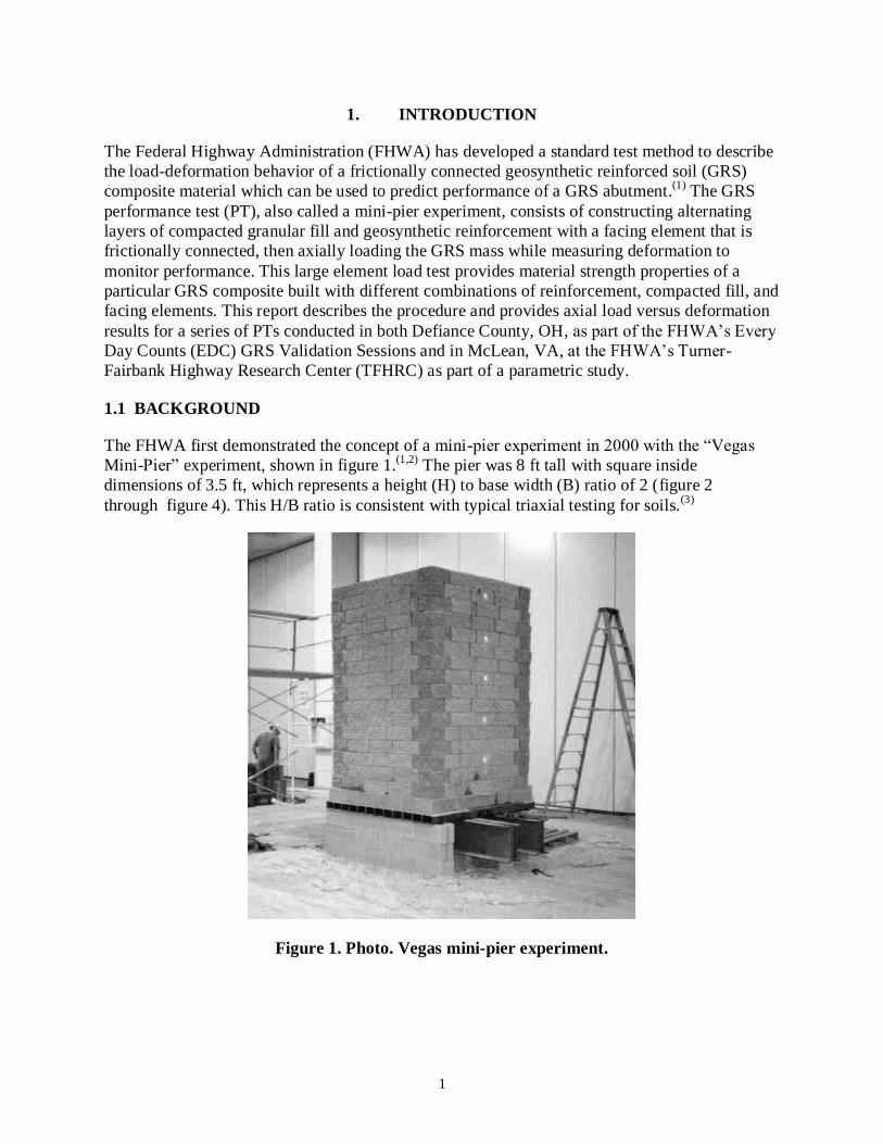
The FHWA first demonstrated the concept of a mini-pier experiment in 2000 with the “Vegas
Mini-Pier” experiment, shown in figure 1.(1,2)
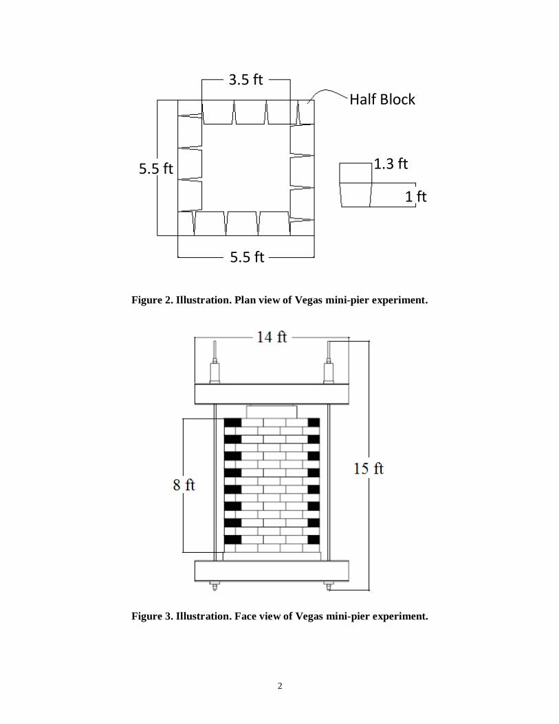
The pier was 8 ft tall with square inside
dimensions of 3.5 ft, which represents a height (H) to base width (B) ratio of 2 (figure 2
through figure 4). This H/B ratio is consistent with typical triaxial testing for soils.(3)
Figure 1. Photo. Vegas mini-pier experiment.
2
Figure 2. Illustration. Plan view of Vegas mini-pier experiment.
Figure 3. Illustration. Face view of Vegas mini-pier experiment.

3
Figure 4. Illustration. Side view of Vegas mini-pier experiment.
The materials used for the GRS pier were a poorly graded-silty gravel (GP-GM, according to the
Unified Soil Classification System, or USCS) soil with a 2,400 lb/ft (ultimate wide width tensile
strength) geotextile spaced every 6 inches frictionally connected to segmental retaining wall
(SRW) blocks for the facing. The top two courses of block, 1 ft from the top of the mini-pier, had
two intermediate bearing bed reinforcement layers as shown in figure 5. The resulting pier was
loaded up to 146 psi; however, time constraints and stroke limitations for the jacks prevented
loading to failure of the composite. Since then, several additional performance tests have been
completed, with the largest load carrying capacity reported at 176 psi.(4,5)

4
Figure 5. Illustration. Reinforcement schedule for Vegas mini-pier experiment.
The concept of testing GRS material has been previously applied on smaller scale models
ranging from small triaxial sized samples to 2-ft cubed specimens in smaller capacity test
frames.(6,7)
Several large scale tests have also been conducted.(7,8,9)
For the aggregates
recommended by FHWA for bridge support, large scale tests are required to adequately predict
performance of a full-scale GRS abutment.(1)
The proposed FHWA PT has been shown to
accurately predict both the strength limit and the service limit for GRS abutments.(5)
1.2 CURRENT PERFORMANCE TESTS
To investigate GRS material further, the FHWA conducted a series of 19 PTs as part of this
research. The layout for these PTs was a slight modification of the Vegas Mini-Pier experiment.
Since these tests were conducted with concrete masonry units (CMU) for the facing, as opposed
to SRW blocks used in the Vegas PT, different test dimensions were needed to retain the H/B
ratio of 2 throughout testing. For CMUs, the typical performance test is 6.4 ft tall with square
inside dimensions of 3.2 ft (figure 6 and figure 7). The parameters that varied among tests were
reinforcement spacing (from 4 to 16 inches), geotextile strength (from 1,400 to 4,800 lb/ft, soil
type (open-graded and well-graded), and frictionally connected facing element (concrete
masonry unit facing and no facing).

5
Figure 6. Illustration. Plan view of Defiance County experiment.
Figure 7. Illustration. Elevation view of Defiance County (DC) test.
1.3 INTERNAL STABILITY DESIGN
The results of the PT are primarily used in the design of GRS abutments.(1)
The resulting stress-
strain curve can be used to describe the strength limit state for capacity and the service limit state
for deformation (vertical and lateral) due to an applied load. It is the only method currently
available to describe both the capacity and deformation behavior of GRS for load bearing
applications; American Association of State Highway and Transportation Officials (AASHTO)
(2012) does not provide any guidance for these GRS limit states.(10)
6
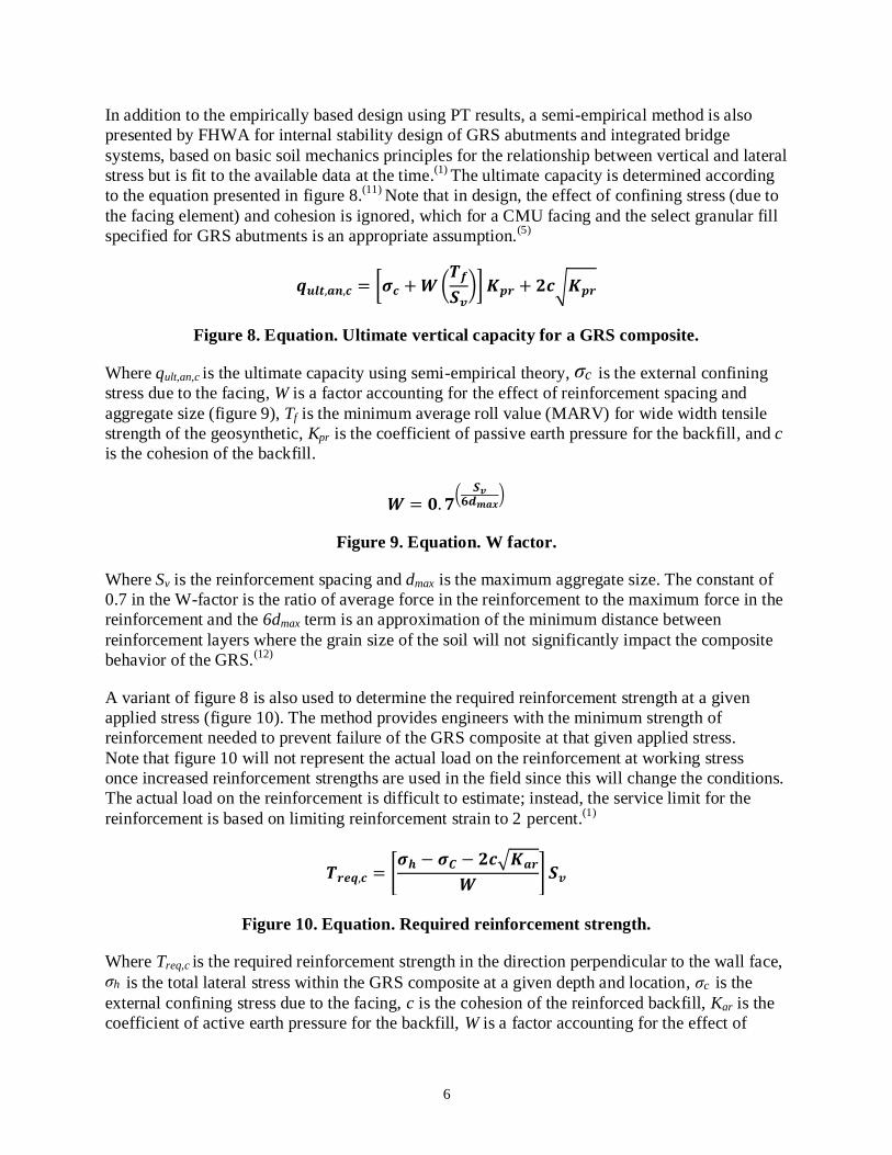
In addition to the empirically based design using PT results, a semi-empirical method is also
presented by FHWA for internal stability design of GRS abutments and integrated bridge
systems, based on basic soil mechanics principles for the relationship between vertical and lateral
stress but is fit to the available data at the time.(1)
The ultimate capacity is determined according
to the equation presented in figure 8.(11)
Note that in design, the effect of confining stress (due to
the facing element) and cohesion is ignored, which for a CMU facing and the select granular fill
specified for GRS abutments is an appropriate assumption.(5)
Figure 8. Equation. Ultimate vertical capacity for a GRS composite.
Where qult,an,c is the ultimate capacity using semi-empirical theory, is the external confining
stress due to the facing, W is a factor accounting for the effect of reinforcement spacing and
aggregate size (figure 9), Tf is the minimum average roll value (MARV) for wide width tensile
strength of the geosynthetic, Kpr is the coefficient of passive earth pressure for the backfill, and c
is the cohesion of the backfill.
Figure 9. Equation. W factor.
Where Sv is the reinforcement spacing and dmax is the maximum aggregate size. The constant of
0.7 in the W-factor is the ratio of average force in the reinforcement to the maximum force in the
reinforcement and the 6dmax term is an approximation of the minimum distance between
reinforcement layers where the grain size of the soil will not significantly impact the composite
behavior of the GRS.(12)
A variant of figure 8 is also used to determine the required reinforcement strength at a given
applied stress (figure 10). The method provides engineers with the minimum strength of
reinforcement needed to prevent failure of the GRS composite at that given applied stress.
Note that figure 10 will not represent the actual load on the reinforcement at working stress
once increased reinforcement strengths are used in the field since this will change the conditions.
The actual load on the reinforcement is difficult to estimate; instead, the service limit for the
reinforcement is based on limiting reinforcement strain to 2 percent.(1)
Figure 10. Equation. Required reinforcement strength.
Where Treq,c is the required reinforcement strength in the direction perpendicular to the wall face,
is the total lateral stress within the GRS composite at a given depth and location, is the
external confining stress due to the facing, c is the cohesion of the reinforced backfill, Kar is the
coefficient of active earth pressure for the backfill, W is a factor accounting for the effect of
𝒒𝒖𝒍𝒕,𝒂𝒏,𝒄 = 𝝈𝒄 + 𝑾 𝑻𝒇
𝑺𝒗 𝑲𝒑𝒓 + 𝟐𝒄 𝑲𝒑𝒓
σc
𝑾 = 𝟎. 𝟕
𝑺𝒗𝟔𝒅𝒎𝒂𝒙
𝑻𝒓𝒆𝒒,𝒄 = 𝝈𝒉 − 𝝈𝑪 − 𝟐𝒄 𝑲𝒂𝒓
𝑾 𝑺𝒗
σh σc

7
reinforcement spacing and aggregate size (figure 9), and Sv is the reinforcement spacing. As with
the ultimate capacity equation, the effect of confining stress (due to the facing element) and
cohesion is ignored when determining the required reinforcement strength in the design of GRS
abutments, leading to added conservatism in the design method.(5)
The soil-geosynthetic composite capacity equation (figure 8) and the required reinforcement
strength equation (figure 10) have been previously validated against the results of 16 different
types of tests, including previous performance tests (figure 12 and figure 13, respectively). The
research study presented in this report will add to this database to further quantify the predictive
capability of these equations.
Note that the predictions for capacity and required reinforcement strength used the estimated
confining stress calculated according to figure 11, and the measured cohesion from soil testing,
both of which would be ignored in design. In addition, the minimum average roll value (MARV)
for the reinforcement, which is a property value calculated as the average strength for a roll less
two standard deviations, was used to calibrate the predictive equations since the actual strength
of the reinforcement for each test was not measured or precisely known, and the MARV is an
industry value common for all geosynthetics specified in practice.
Figure 11. Equation. Confining stress.(11)
Where is the bulk unit weight of the facing block, d is the depth of the facing block unit
perpendicular to the wall face, and is the interface friction angle between the geosynthetic and
the facing element for a frictionally connected GRS composite.
Note that the friction angle and cohesion terms used to calculate the earth pressure coefficients
and lateral stress within the ultimate capacity (figure 8) and required reinforcement strength
(figure 10) equations were measured using a large scale direct shear (LSDS) test on the backfill
alone according to ASTM D3080.(13)
The peak strength of the reinforced backfill material was
selected as it is a commonly reported value and easiest to ascertain from typical testing. More
details are provided in section 2.1.3.
𝝈𝒄 = 𝜸𝒃𝒅𝒕𝒂𝒏𝜹
γb
δ

8
Figure 12. Graph. Predictive capability of the soil-geosynthetic
composite capacity equation.(5)
Figure 13. Graph. Predictive capability of the required reinforcement strength equation.(5)

9
1.4 OBJECTIVES
The results of the PT parametric study will be used for several purposes. The primary objectives
of this research report are to: (1) build a database of GRS material properties that can be used by
designers or for Load and Resistance Factor Design (LRFD) calibration; (2) evaluate the
relationship between reinforcement strength and spacing; (3) quantify the contribution of the
frictionally connected facing elements at the service limit and strength limit states; (4) assess the
new internal stability design method proposed by Adams et al. 2011a for GRS; and (5) perform a
reliability analysis of the proposed soil-geosynthetic capacity equation for LRFD.(1,11)
When
combining additional measurement techniques (e.g., contact pressure cells, earth pressure cells,
etc.), other uses for the PT are possible, such as to study thrust against the face as a function of
spacing; however, this is outside the scope of this report.


11
2. TESTING CONDITIONS
A series of 19 performance tests have been conducted (table 1); 5 at the Defiance County, OH,
highway maintenance facility and 14 at the TFHRC.
Table 1. Summary of PT conditions.
Test
No.
Backfill Reinforcement
Facing
Type (°)
c
(psf)
dmax
(inch)
Tf^
(lb/ft)
Sv
(inch)
Tf/Sv
(lb/ft2)
DC-1 8 54 0 ½ 4,800 7⅝** 7,600 CMU
DC-2 8P* 46 0 ¾ 4,800 7⅝** 7,600 CMU
DC-3 57 52 0 1 4,800 7⅝** 7,600 CMU
DC-4 9 49 0 ⅜ 4,800 7⅝** 7,600 CMU
DC-5 8*** 54 0 ½ 4,800 7⅝** 7,600 CMU
TF-1++
8 55 0 ½ 2,400 7⅝ 3,800 CMU
TF-2 21A 53 115 1 2,400 7⅝ 3,800 CMU
TF-3 21A 53 115 1 2,400 7⅝ 3,800 no CMU
TF-4+ 21A 53 115 1 4,800 7⅝ 7,600 no CMU
TF-5++
21A 53 115 1 4,800 7⅝ 7,600 no CMU
TF-6++
21A 53 115 1 4,800 7⅝ 7,600 CMU
TF-7 21A 53 115 1 4,800 7⅝ 7,600 no CMU
TF-8 21A 53 115 1 4,800 7⅝** 7,600 no CMU
TF-9 21A 53 115 1 4,800 15¼ 3,800 CMU
TF-10 21A 53 115 1 4,800 15¼ 3,800 no CMU
TF-11 21A 53 115 1 1,400 313
/16 4,400 no CMU
TF-12 21A 53 115 1 1,400 313
/16 4,400 CMU
TF-13 21A 53 115 1 3,600 11¼ 3,800 no CMU
TF-14 21A 53 115 1 3,600 11¼ 3,800 CMU
ϕ = the peak friction angle, c = the cohesion at peak strength, dmax = the maximum aggregate
size, Tf = the ultimate reinforcement strength, expressed as the minimum average roll value
(MARV) from ASTM D4595 testing,(1)
and Sv = the reinforcement spacing. ^ MARV value.
*Rounded pea-gravel angularity.
**Two courses of bearing bed reinforcement placed at the top of the PT.
***Uncompacted sample, +technical difficulties required termination during testing.
++Technical difficulties resulted in unloading/reloading of the composite.
2.1 BACKFILL CONDITIONS
In total, six unique backfill types were used in the PTs: (1) an AASHTO No. 8 crushed,
manufactured limestone aggregate obtained from Defiance County OH, (2) an AASHTO No. 8
rounded quartz pea gravel (PG) obtained from Defiance County, OH, (3) an AASHTO No. 57
crushed, manufactured limestone aggregate obtained from Defiance County, OH, (4) an
AASHTO No. 9 crushed, manufactured limestone aggregate obtained from Defiance County,
ϕ

12
OH, (5) an AASHTO No. 8 crushed, manufactured diabase aggregate obtained from Loudon
County, VA, and (6) an AASHTO A-1-a aggregate obtained from Loudon County, VA (also
referred to locally as a Virginia DOT, or VDOT, 21A material).
2.1.1 Sieve Analysis
All backfills used for testing, except for the AASHTO No. 9 aggregates, meet the FHWA
specifications for use in bridge abutments.(1)
The gradations of each aggregate are shown in
table 2 and figure 14.
Table 2. PT reinforced backfill gradations.
Sieve
No.
Percent Passing
No. 8
(OH)
No. 8 PG
(OH)
No. 57
(OH)
No. 9
(OH)
No. 8
(VA)
A-1-a
(VDOT 21A)
1.5 100.00 100.00 100.00
1 100.00 100.00 100.00
0.75 100.00 100.00 87.91
0.50 100.00 99.57 35.69 99.69 82.41
0.375 96.99 95.58 14.13 100.00 69.86 71.36
4 26.50 14.60 3.67 94.22 7.78 48.52
8 4.63 6.98 2.41 27.75 1.66 35.24
10 1.39 32.81
16 1.85 4.34 1.47 8.90 1.11 25.40
40 0.93 16.66
50 0.91 2.64 3.66 0.88
100 0.76 3.22
200 0.65 0.71 2.82 6.47
Blank cell = no value was measured for that particular sieve number.
Most of the backfills tested are open or poorly graded materials (e.g., AASHTO Nos. 57, 8,
and 9); however, the A-1-a material is a well-graded material. Table 3 shows the classification
(based on the USCS) along with the maximum aggregate size (dmax), other relevant grain sizes
for various percent passing values, and the coefficient of curvature (Cc) and coefficient of
uniformity (Cu) for each material tested.

13
Table 3. PT backfill gradation properties.
Aggregate
Type
USCS
Classification
dmax
(inch)
D85
(inch)
D60
(inch)
D30
(inch)
D10
(inch) Cc Cu
8 (OH) GP 0.50 0.34 0.28 0.20 0.12 1.19 2.36
8 PG (OH) GP 0.75 0.35 0.29 0.22 0.13 1.30 2.23
57 (OH) GP 1.00 0.74 0.62 0.47 0.30 1.18 2.05
9 (OH) SP 0.38 0.17 0.14 0.47 0.05 1.35 2.78
8 (VA) GP 1.00 0.44 0.35 0.25 0.19 0.96 1.78
A-1-a
(VDOT 21A)
GW-GM 1.00 0.57 0.28 0.07 0.01 2.67 46.67
dmax = the maximum aggregate size.
D85 = the aggregate size in which 85 percent of the sample is finer.
D60 = the aggregate size in which 60 percent of the sample is finer.
D30 = the aggregate size in which 30 percent of the sample is finer.
D10 = the aggregate size in which 10 percent of the sample is finer.
Cc = the coefficient of curvature.
Cu = the coefficient of uniformity.

14
Figure 14. Graph. Reinforced backfill gradations.

15
2.1.2 Density
To determine the in-place compaction requirements of the backfill material, a standard Proctor
test was conducted according to Method D of AASHTO T99 for the AASHTO A-1-a (VDOT
21A) material.(15)
In addition, vibratory tests were conducted according to ASTM D4252 for the
open-graded materials to determine the maximum dry density.(16)
The results are shown in
table 4.
Table 4. Maximum dry density for PT aggregates.
Aggregate Type
Max Dry Density,
(pcf)
Optimum Moisture Content,
(percent)
8 (OH) 101.27 N/A
8 PG (OH) 115.75 N/A
57 (OH) 108.69 N/A
9 (OH) 110.66 N/A
8 (VA) 112.82 N/A
A-1-a (VDOT 21A) 148.90 7.7
N/A = Not applicable, there is no optimum moisture content for open-graded aggregates
since they are free draining.
2.1.3 Friction Angle
The strength properties of each aggregate were determined using a large scale direct shear
(LSDS) device according to ASTM D3080.(13)
The LSDS device at TFHRC is 12 x 12 x 8 inches
in dimension and is capable of testing aggregates up to 1.2 inches. For this series of experiments,
the unscalped aggregates were tested at four applied normal stresses, 5, 10, 20, and 30 psi, at a
shear rate of 0.015 inches/min and a gap size equal to the D85 of the material (i.e., the aggregate
size where 85 percent of the sample is smaller; see table 3).
The open-graded materials were tested in a dry, uncompacted state prior to the consolidation
phase in the LSDS device. The well-graded material (VDOT 21A) was tested at 100 percent of
the maximum dry density (i.e., the level of compaction achieved during each PT with the
backfill), and at the optimum moisture content (see table 4). Since the shear strength failure
envelope for these aggregates is non-linear, the reported cohesion for the well-graded material
(VDOT21A) was determined through a series of LSDS tests that were performed with the
compacted state fully saturated; note that the resulting peak friction angle in this case was similar
to the non-saturated condition.
The results of the LSDS testing are shown in table 5 and in figure 15. Note that the reported
friction angle is based on the measured peak strength during testing and assumes a linear Mohr-
Coulomb envelope for the range of confining stresses tested. Note that peak strength for these
backfill materials is mobilized at typically 0.5- to 1-inch lateral displacement in the LSDS
device, which corresponds to about 4- to 8-percent lateral strain for the 12-inch shear box. In the
context of the PT though, the GRS composite is tested to failure, sometimes well beyond
8-percent lateral strain. From a theoretical perspective, it may be more appropriate to model the
γd ω

16
failure of a GRS composite by using the friction angle at the fully softened state of the backfill
material during the LSDS test; however, to conform to the current standard-of-practice, the peak
strength of the reinforced backfill material was selected to calibrate the design as it is the
commonly reported value and easiest to ascertain from typical testing. Figure 15 provides the
raw data for LSDS testing.
Table 5. LSDS testing results.
Aggregate Type Friction Angle (°) Cohesion (psf)
8 (OH) 54 0
8 PG (OH) 46 0
57 (OH) 52 0
9 (OH) 53 0
8 (VA) 55 0
A-1-a (VDOT 21A) 54 115
Figure 15. Graph. LSDS testing results.
0
10
20
30
40
50
60
0 5 10 15 20 25 30 35 40
Sh
ear
Str
ess
(p
si)
Normal Stress (psi)
No. 8 (OH)
No. 8 PG (OH)
No. 57 (OH)
No. 9 (OH)
No. 8 (VA)
VDOT 21A
VDOT 21A (Saturated)

17
2.2 REINFORCEMENT CONDITIONS
In all of the tests, a biaxial, woven polypropylene geotextile was used as the reinforcement
element; however, different strengths and stiffness of material were used among the PTs. The
manufacturer supplied MARV data is shown in table 6. A more recent property of the
geosynthetic used in design is the wide width tensile strength at 2-percent strain which provides
an indication of GRS performance at the service limit state.(1)
Currently, many of the
manufacturers do not make this value publicly available, although they can supply it on request.
Note that in the field, the actual strength of the reinforcement will be higher than the reported
MARV.
Table 6. Geosynthetic reinforcement properties.
PTs:
TF-11,
TF-12
TF-1,
TF-2,
TF-3
TF-13,
TF-14
DC-1, DC-2,
DC-3, DC-4,
DC-5, TF-4,
TF-5, TF-6,
TF-7, TF-8,
TF-9, TF-10
Reference: (17) (18) (19) (18)
Property Test
Method Minimum Average Roll Value (MARV)
1
Tensile
Strength
(Grab)
ASTM
D4632(20)
200 x 200 lb 315 x 300 lb 450 x 350 lb 600 x 500 lb
Wide
Width
Tensile
ASTM
D4595(14)
1,400 x
1,400 lb/ft
2,400 x
2,400 lb/ft
3,600 x 3,600
lb/ft
4,800 x
4,800 lb/ft
Wide
Width
Elongation
ASTM
D4595(14)
9 x 7 percent
10 x 8
percent 15 x 10 percent
10 x 8
percent
Wide
Width
Tensile
Strength at
5 Percent
Strain
ASTM
D4595(14)
Not
specified
884 x 1,564
lb/ft
1,392 x 1,740
lb/ft
660 x 1,500
lb/ft
1Values for the machine (warp) by cross machine (fill) directions, respectively.
2.3 FACING CONDITIONS
A concrete masonry unit (CMU) facing was used on 11 of the 17 tests; the remaining 6 tests
were conducted without any facing element. The CMU is a dry-cast, split-faced product with
dimensions of 7⅝ x 7⅝ x 15⅝ inches and an approximate weight of 42 lb. The CMUs are
frictionally connected to the geotextile reinforcement. The reinforcement overlaps at least
85 percent of the block depth, termed the coverage ratio, as specified by Adams et al. 2011a.(1)


19
3. TEST SETUP
3.1 LAYOUT
The dimensions for each PT are given in table 7. For each test, the base to height ratio was kept
constant at about 2 to mimic triaxial conditions. The height is equivalent to 10 courses of CMU
block, while the outside dimensions of the PT with facing are 3.5 blocks wide. For each test, the
total width of the PT with the CMU facing (Btotal) is 54½ inches; the width of the GRS composite
itself (B) is 39¼ inches. The footing width on top of the GRS composite (b) is 36 inches.
Table 7. PT dimensions.
Test No No. Reinf. Layers
Sv
(inch)
H
(inch) H/B
DC-1 9 7⅝** 76¼ 1.9
DC-2 9 7⅝** 76¼ 1.9
DC-3 9 7⅝** 76¼ 1.9
DC-4 9 7⅝** 76¼ 1.9
DC-5 9 7⅝** 76¼ 1.9
TF-1 9 7⅝ 76¼ 1.9
TF-2 9 7⅝ 76¼ 1.9
TF-3 9 7⅝ 76¼ 1.9
TF-4 9 7⅝ 76¼ 1.9
TF-5 9 7⅝ 76¼ 1.9
TF-6 9 7⅝ 76¼ 1.9
TF-7 9 7⅝ 76¼ 1.9
TF-8 9 7⅝** 76¼ 1.9
TF-9 4 15¼ 76¼ 1.9
TF-10 4 15¼ 76¼ 1.9
TF-11 19 313
/16 76¼ 1.9
TF-12 19 313
/16 76¼ 1.9
TF-13 6 11¼ 78¾ 2.0
TF-14 6 11¼ 78¾ 2.0
Sv = the reinforcement spacing, H = the height of the PT,
B = the width of the GRS composite (without the facing
element).
**Two courses of bearing bed reinforcement placed at the top
of the PT.

20
Figure 16. Photo. DC-1 GRS PT (before testing).
3.2 LOAD AND REACTION FRAME
The reaction frames were slightly different among the tests. The Defiance County PTs (DC-1
through DC-5) were built on a reinforced concrete base pad similar to the Vegas mini-pier setup
(figure 3 and figure 4). The base pad was elevated on CMU blocks to make room for the bottom
set of bolted channel beams, while the top set of bolted channels was supported on the top
concrete pad which was centered on the GRS composite. The top load pad is supported on the
GRS composite, inside the perimeter of the CMU facing; there is an inset of 1⅝ inches around
the load pad and the back of the CMU facing (figure 17). The upper and lower channel beams
were coupled together with high strength post-tensioning bar. Four hollow core hydraulic jacks
were bolted to the top channel beams (figure 18). All jacks were connected to a manifold and
controlled with an electric hydraulic pump controlled by a push button solenoid valve. The
stroke and capacity of the hollow core jacks were 6 inches and 120 kips, respectively.

21
Figure 17. Illustration. Concrete footing on GRS composite, inset from facing.
Figure 18. Photo. Hollow core hydraulic jacks for PT assembly.
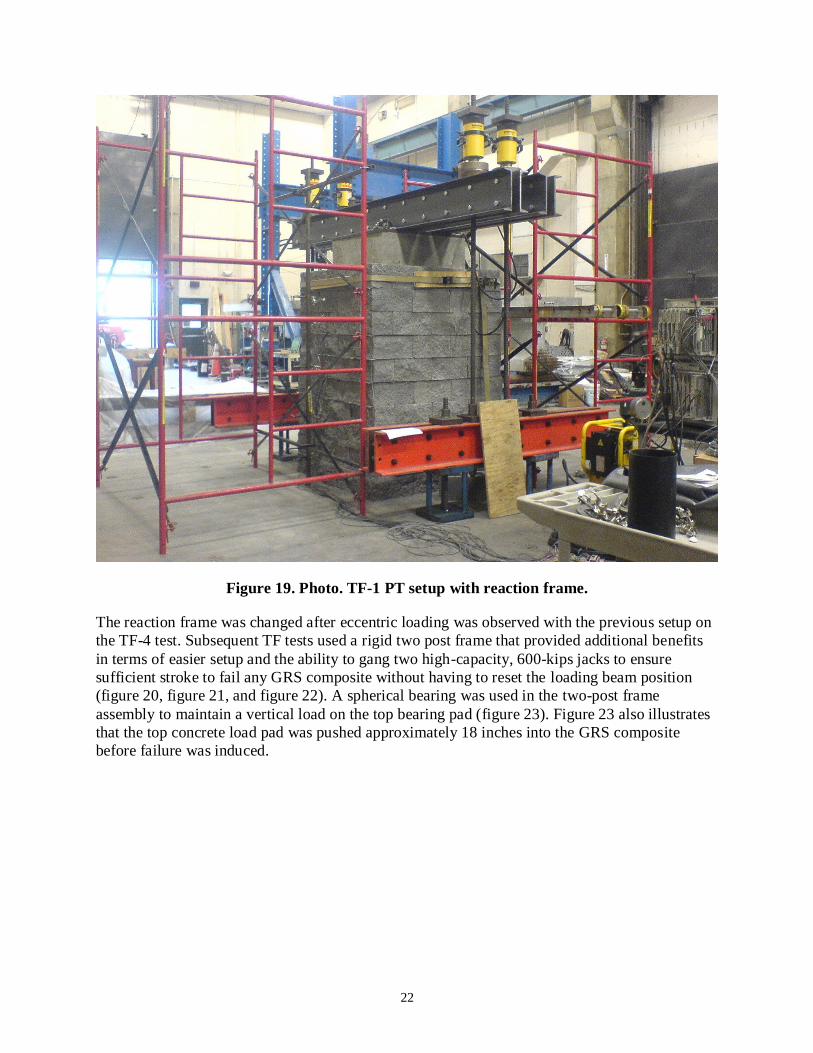
A similar reaction frame setup was used for the initial TFHRC PTs (figure 19), except the
concrete strong floor was used for the reaction instead of sandwiching the GRS composite
between twin sets of bolted channels (figure 4). The top sets of bolted channels were placed on
an elastomeric pad and positioned on the top concrete pad to evenly distribute the load delivered
from the hydraulic jacks; a 1-inch steel plate was also bolted to the top concrete pad to increase
the rigidity of the concrete.
22
Figure 19. Photo. TF-1 PT setup with reaction frame.
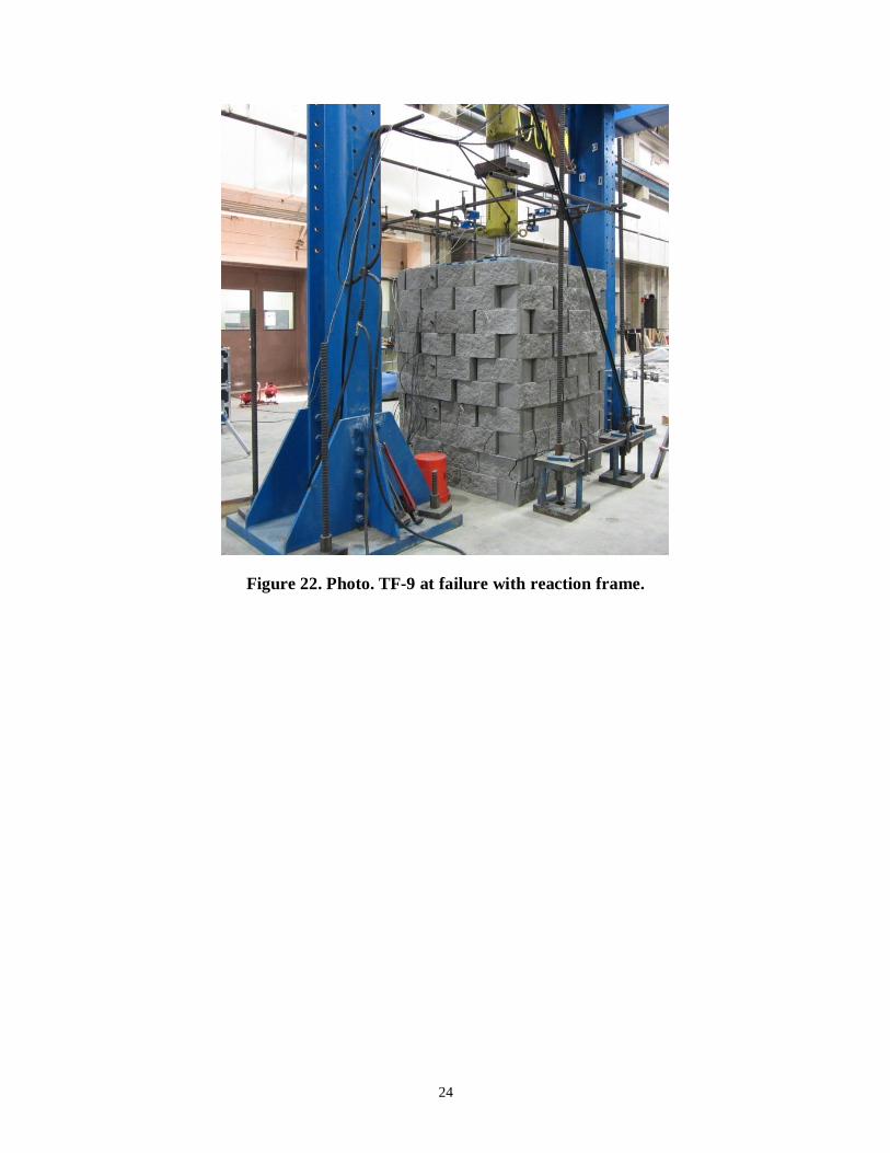
The reaction frame was changed after eccentric loading was observed with the previous setup on
the TF-4 test. Subsequent TF tests used a rigid two post frame that provided additional benefits
in terms of easier setup and the ability to gang two high-capacity, 600-kips jacks to ensure
sufficient stroke to fail any GRS composite without having to reset the loading beam position
(figure 20, figure 21, and figure 22). A spherical bearing was used in the two-post frame
assembly to maintain a vertical load on the top bearing pad (figure 23). Figure 23 also illustrates
that the top concrete load pad was pushed approximately 18 inches into the GRS composite
before failure was induced.
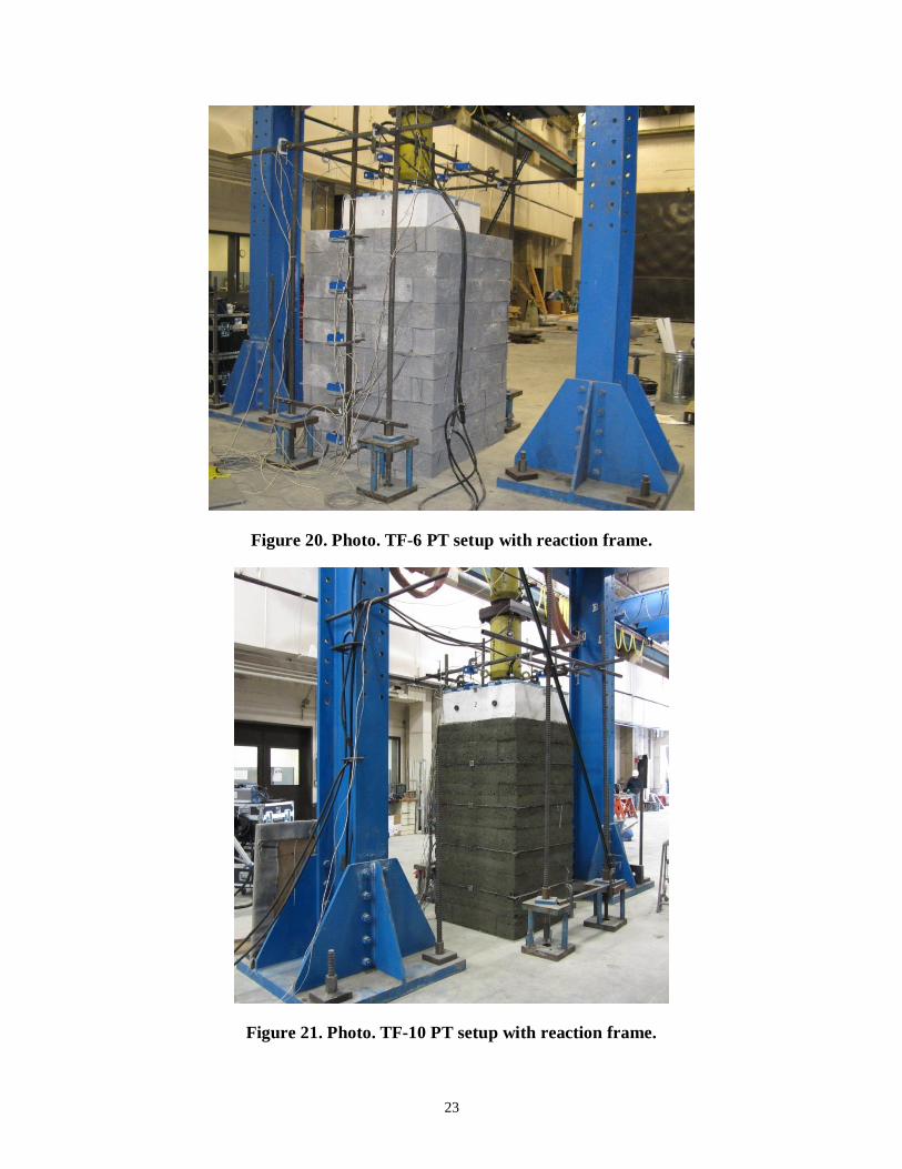
23
Figure 20. Photo. TF-6 PT setup with reaction frame.
Figure 21. Photo. TF-10 PT setup with reaction frame.
24
Figure 22. Photo. TF-9 at failure with reaction frame.

25
Figure 23. Photo. Spherical bearing to apply load to the footing on the GRS composite.
3.3 CONSTRUCTION
The method of construction for the mini piers was basically the same for all of the PTs; the GRS
composite was built from the bottom up, one course of block at a time. The primary difference in
construction between the Defiance County tests and the TFHRC tests was the level of quality
control. The five Defiance County tests (DC-1 through DC-5) were each constructed with the
same supervisor, but different crews, as part of the FHWA’s EDC-GRS Validation Sessions in
2010. The quality control for these tests was therefore limited, which may have impacted the
testing results, particularly the stiffness. The 14 PTs conducted at TFHRC were constructed in
the Structures Laboratory and were research quality experiments, with consistent construction
procedures and compaction control.
At the start of construction for each PT, the first course of block was placed level and centered
within the position of the reaction assembly. Aggregate was then infilled using either a front-end
loader (for the DC test series) or a concrete dump hopper (for the TF test series). For the TF
tests, the squareness of the facing and the verticality of the composite were checked before
placement of fill in each course of block by measuring the inside diagonal lengths and checking
with a plumb bob on every other lift.
Compaction for the DC tests was performed using a standard 18-inch-wide, gas powered
vibratory plate compactor at each lift of aggregate, a nominal 8-inch thickness (height of the
CMU block). For the TF tests, it was necessary to compact each 8-inch lift of fill in half layer
increments, or at a lift thickness of about 4 inches because a lightweight electric vibratory plate
compactor was used for construction; with this equipment, it was impossible to achieve the target

26
density at the nominal 8-inch lifts. The electric compactor had a 10-square-inch plate, with a
weight of 48 lb and an adjustable impact force of 700 lb.
For the well-graded AASHTO A-1-a (VDOT 21A) aggregate, compaction control consisted of
testing each nominal 4-inch lift (half the height of a CMU) with a nuclear density gauge to
ensure the target density and moisture content (± 2 percent) were met throughout the height of
the GRS composite. In the field, density tests are typically performed after the compaction of fill
material to the height of CMU block; however, during construction of the TF PTs using well-
graded backfill, density testing was performed on nominal 4-inch lifts to test the compaction
effort of the lightweight (48 lb) tamper used. For each lift, approximately 100 percent of the
standard Proctor value was achieved; the results of the nuclear density gauge for each test are
shown in appendix B.
For the open-graded aggregates, compaction was performed until no further compression of the
aggregate was observed, which consisted of running the plate compactor across each lift with a
minimum of four passes. While it is not common practice to test open-graded aggregates with a
nuclear density gauge, backscatter tests were performed on each nominal 4-inch lift for PT TF-1
to collect the surficial density value (appendix B). The percent compaction is based on the
maximum index density determined from ASTM D4253 (table 4).(16)
Rodding with a shovel end was also used for each PT to compact the aggregate at the corners and
edges of the facing. Once final compaction was achieved to the leveled height of the facing block
and before placement of the next course of CMU blocks, any remaining aggregate was brushed
off of the facing block so that a smooth surface existed to prevent point loading and ensure even
placement of the next layer of block. Depending on the reinforcement schedule, a layer of
geotextile reinforcement was then placed over the aggregate with a facing element coverage ratio
of at least 85 percent the width of facing element. While the geotextiles used in each test were
biaxial, the stiffness in the machine (warp) and cross-machine (fill) directions for the
reinforcement was different (table 6). For this reason, the reinforcement was placed in an
alternating pattern with each subsequent layer to prevent preferential failure of the PT in the
weaker reinforcement direction.
To facilitate construction, two sets of ratchet straps were placed around the facing blocks to
secure and maintain block alignment during compaction. During each layer of GRS construction,
the lower strap was removed and then used to band the new, upper course of block; the process
was repeated until the pier was completed. This process was employed because of the geometry
and the reduced footprint of the PT where lateral block movement during compaction is
increased compared to a typical in-service bridge abutment (plane strain condition). The ratchet
strap on the top course of block was removed after specimen construction was fully completed,
prior to loading.
Once the fabric was placed, the next layer of CMU blocks were positioned and the aggregate
infilled. This process was repeated for 10 courses of CMU blocks. The concrete footing was then
placed on top of the GRS composite and the load frame assembled for testing. Construction of
the open-graded aggregate tests took about 4 hours, and 20 hours for the DC tests and TF tests,
respectively. The principal difference in time was attributable to the need for compaction in

27
4-inch lifts, the requirement for nuclear density testing, and the level of quality control.
Construction of the well-graded aggregate tests at TF took approximately 30 hours.
3.4 INSTRUMENTATION
Each PT was instrumented to measure the response to the static, vertical applied pressure on the
top of the GRS composite. Vertical and lateral deformation was constantly monitored with
displacement transducers. Four transducers measured the vertical displacement at the middle of
each loading block edge while five transducers measured the horizontal displacement along one
face of the specimen (figure 24). For the five PTs conducted in Defiance County, OH, (DC-1
through DC-5) and the first PT conducted at TFHRC (TF-1), linear voltage displacement
transducers (LVDT) were used.
String potentiometers (POT) replaced the LVDTs for the remaining tests at TFHRC with CMU
blocks (TF-2, TF-6, TF-9, TF-12, TF-14) to measure both vertical and lateral deformation. For
the PTs without any facing element (TF-3, TF-4, TF-5, TF-7, TF-8, TF-10, TF-11, TF-13),
LVDTs were still used to measure lateral deformation in addition to the string POTs used to
measure vertical deformation. The instrumentation layouts for deformation measurements in
each test, similar to that shown in figure 24, are presented in appendix C. With the TFHRC PT
series, additional instrumentation was included to monitor vertical pressure near the base of the
composite, strain on different geotextile layers, and lateral earth pressure behind the face just
above the center height of the composite (figure 25). This report focuses on the vertical
deformation data, which can be immediately used in the design of GRS composites for load
bearing applications.(1)
Figure 24. Illustration. Instrumentation layout for DC tests and TF-1.

28
Figure 25. Illustration. General additional instrumentation layout TF PT series.
3.5 LOAD SCHEDULE AND COLLECTION OF DATA
For each TFHRC test, the loading schedule was prepared in the same manner. The basic protocol
included estimating the ultimate vertical capacity determined from the semi-empirical equation
(figure 8). The estimated capacity was then divided into a minimum of ten load increments to
capture the deformation characteristics of each test. In addition, between two and four load
increments below the 4,000 psf service limit were included in each test to better define the
behavior of the composite at low applied loads.
Each load increment was applied manually using an electric hydraulic pump with a push button
controlled solenoid valve. Load was maintained with a strain indicator box calibrated to a load
cell placed within the reaction assembly. Hydraulic jack pressure was also checked at each load
increment to ensure operation of the system throughout the course of the load test. In each
experiment, load was increased, from increment to increment, only when there was no significant
change (< 0.003 inch) in settlement between any two time intervals; however, the load increment
was held for a minimum of 5 minutes and a maximum of 30 minutes. The data acquisition
system was programmed to record settlement at 1-, 3-, 5-, 7-, 15-, 20-, 25-, and 30-minute
intervals from the start of each load increment.
The settlement of the top footing, lateral displacement of the face, and geotextile strain were
recorded every minute within each load increment. Any vertical earth pressure measurements
and lateral stress information were collected at the end of each load increment. Photographs were
also taken at the conclusion of each load increment to visually document the test. Typically, each
test took about 6 hours to complete.

29
4. RESULTS DATABASE
The results for each test are presented in table 8. The corresponding vertical stress-strain curves
are shown in figure 26 and figure 27 for the Defiance County tests (labeled DC) and the TFHRC
tests (labeled TF), respectively. The tabular data for each stress-strain curve shown in figure 26
and figure 27 is given in appendix D. Note that the applied stress and strain are calculated as
averages of the measured values (over the period of loading for stress and over the four
LVDT/POTs located on the footing for strain at the end of each load increment).
Table 8. PT measured results summary.
Maximum Tested
Strength
Limit Design Limit
Service
Limit
Test
No.
qmax
(psf)
(%)
qult,emp
(psf)
(psf)
Vallow,emp =
/3.5 (psf)
(psf)
DC-1 23,310 7.95 23,310 19,983 5,709 3,065
DC-2 22,709 7.07 22,709 19,399 5,543 2,171
DC-3 18,447 5.82 N/A 16,182 4,623 1,324
DC-4 26,730 7.64 N/A 17,350 4,957 2,212
DC-5 21,539 10.42 21,539 11,761 3,360 316
TF-1 20,487 10.9 20,487 13,409 3,831 2,075
TF-2 25,260 11.46 25,260 18,711 5,346 4,759
TF-3 17,491 13.8 17,491 12,120 3,463 3,417
TF-4 14,240 4.4 N/A N/A1 N/A
1 3,705
TF-5 25,920 17.9 25,920 15,581 4,452 1,815
TF-6 43,828 15.7 43,828 22,007 6,288 3,704
TF-7 26,546 12.5 26,546 13,684 3,910 2,224
TF-8 29,134 17.8 29,134 13,797 3,942 1,753
TF-9 22,310 15.6 22,310 13,527 3,865 2,955
TF-10 10,330 14.27 10,330 7,374 2,107 1,586
TF-11 23,249 12.79 23,249 13,316 3,805 2,839
TF-12 29,030 13.37 29,030 18,573 5,307 4,028
TF-13 12,960 12.32 12,960 8,641 2,469 2,398
TF-14 23,562 12.69 23,562 16,748 4,785 2,037
qmax = the maximum applied pressure during testing, = the maximum recorded vertical
strain, qult,emp is the measured failure pressure, = the applied stress at 5 percent
vertical strain, Vallow,emp is the total allowable pressure on the GRS,(1)
= the applied
stress at 0.5 percent vertical strain.
N/A = Not applicable, did not fail composite. N/A1 = Not applicable, composite did not reach
5-percent vertical strain before it was terminated.
εmax q@ε=5% q@ε=5%
q@ε=0.5%
εmax
q@ε=5%
q@ε=0.5%

30
Figure 26. Graph. Load-deformation behavior for the Defiance County PTs.

31
Figure 27. Graph. Load-deformation behavior for the Turner Fairbank PTs.

32
Note that two Defiance County (DC-3 and DC-4) and one TFHRC test (TF-4) were prematurely
terminated before failure of the GRS composite. For the DC tests, the 6-inch stroke of the
hydraulic jacks limited the amount of deformation that could be applied to the samples without
resetting the experiment, which did not occur. For the TF test, the applied load on TF-4 was not
uniform, leading to tilting of the footing (figure 28). Analysis of the data shows this to be the
case.
Figure 28. Photo. Tilting of the footing during TF-4 testing.
The TF-4 data plotted on the family of load test curves shown in figure 27 is the average
measured settlement from the four string POTs located on each side of the top of the footing.
Figure 29 shows the settlement data for each POT, along with the average, for the TF-4 test. As
indicated visually (figure 28), the measurements (figure 29) confirm that the footing titled
towards sides 3 and 4 of the footing. Figure 28 also illustrates the composite behavior of GRS
(i.e., the soil and geosynthetic tend to move together as one material).

33
Figure 29. Graph. TF-4 results.
4.1 UNLOAD/RELOAD BEHAVIOR
TF-1, TF-5 and TF-6 experienced technical difficulties during testing that resulted in an
unloading/reloading of the composite (figure 30, figure 31 and figure 32, respectively). The load
test curves shown in figure 27 were corrected to omit the unload/reload cycles.
Due to a power outage at TFHRC during testing for TF-1 (figure 30), the GRS composite was
unloaded for a period of over 40 hours (1.7 days); the maximum applied stress prior to unloading
of the composite was 12,761 psf. After reestablishing power, the sample was then reloaded with
the approximate same loading schedule as the initial load until failure of the composite was
reached at 20,487 psf. The initial ratio of stress to strain (Eo) is equal to approximately 320 ksf,
while the reload response was considerably stiffer by a factor of over 6, with a reload ratio of
stress to strain (ER) around 2,070 ksf.
For TF-5 (figure 31), the GRS composite was initially loaded and reloaded twice at low applied
loads (less than 4,700 psf). The string potentiometers were reset in each case. An additional
unloaded cycle then occurred for a period of 12 minutes 50 seconds in order to reset the single
hollow-core jack because of the stroke limitation (hence, the change to the use of two jacks in
series starting with TF-6). After resetting the jack, the sample was then reloaded at the
approximate same loading schedule as the initial load. The last reload cycle that occurred during
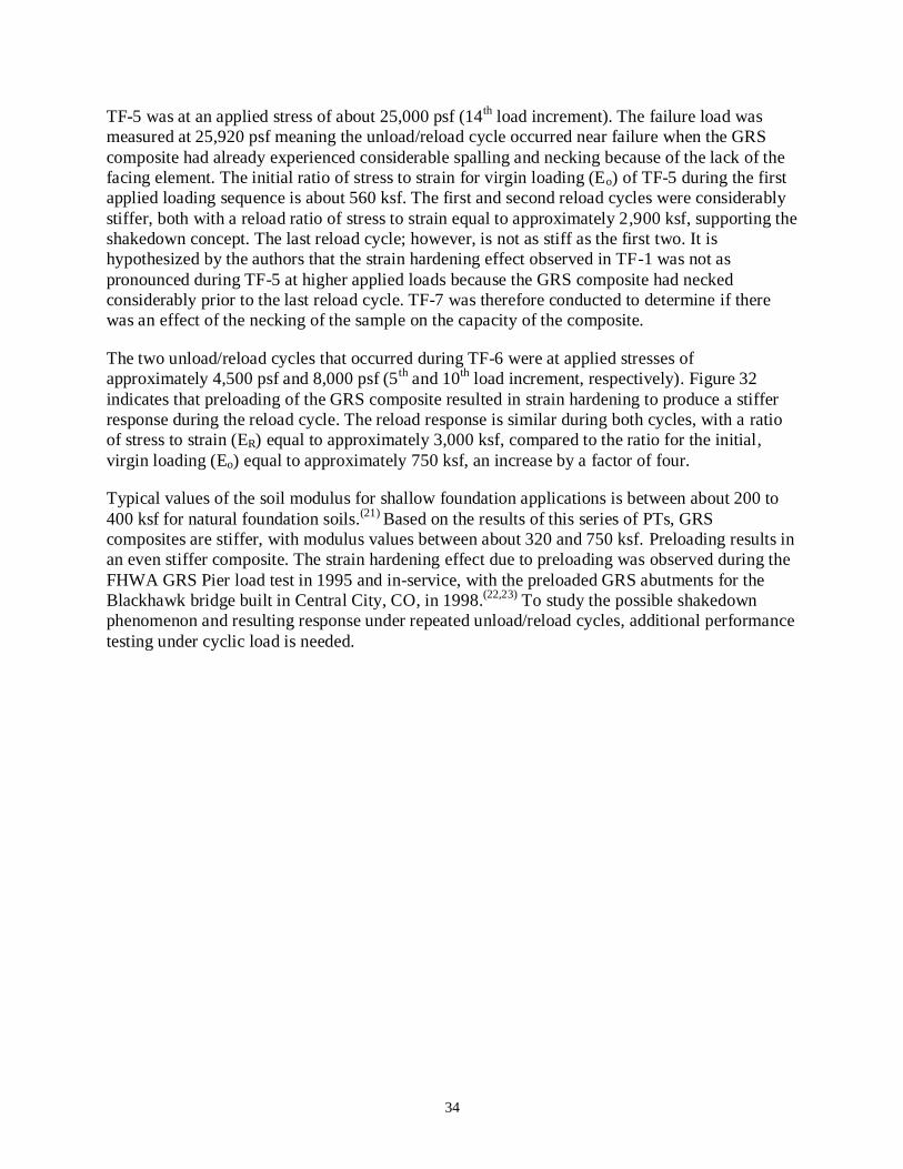
34
TF-5 was at an applied stress of about 25,000 psf (14th
load increment). The failure load was
measured at 25,920 psf meaning the unload/reload cycle occurred near failure when the GRS
composite had already experienced considerable spalling and necking because of the lack of the
facing element. The initial ratio of stress to strain for virgin loading (Eo) of TF-5 during the first
applied loading sequence is about 560 ksf. The first and second reload cycles were considerably
stiffer, both with a reload ratio of stress to strain equal to approximately 2,900 ksf, supporting the
shakedown concept. The last reload cycle; however, is not as stiff as the first two. It is
hypothesized by the authors that the strain hardening effect observed in TF-1 was not as
pronounced during TF-5 at higher applied loads because the GRS composite had necked
considerably prior to the last reload cycle. TF-7 was therefore conducted to determine if there
was an effect of the necking of the sample on the capacity of the composite.
The two unload/reload cycles that occurred during TF-6 were at applied stresses of
approximately 4,500 psf and 8,000 psf (5th
and 10th
load increment, respectively). Figure 32
indicates that preloading of the GRS composite resulted in strain hardening to produce a stiffer
response during the reload cycle. The reload response is similar during both cycles, with a ratio
of stress to strain (ER) equal to approximately 3,000 ksf, compared to the ratio for the initial,
virgin loading (Eo) equal to approximately 750 ksf, an increase by a factor of four.
Typical values of the soil modulus for shallow foundation applications is between about 200 to
400 ksf for natural foundation soils.(21)
Based on the results of this series of PTs, GRS
composites are stiffer, with modulus values between about 320 and 750 ksf. Preloading results in
an even stiffer composite. The strain hardening effect due to preloading was observed during the
FHWA GRS Pier load test in 1995 and in-service, with the preloaded GRS abutments for the
Blackhawk bridge built in Central City, CO, in 1998.(22,23)
To study the possible shakedown
phenomenon and resulting response under repeated unload/reload cycles, additional performance
testing under cyclic load is needed.
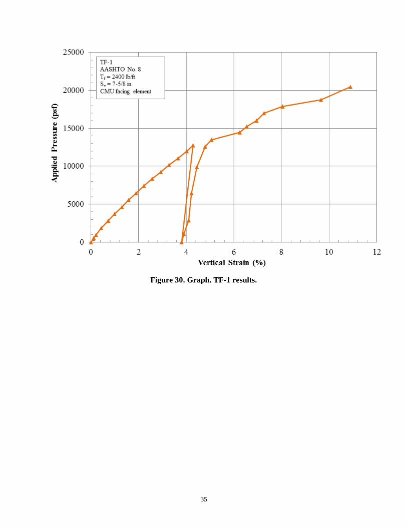
35
Figure 30. Graph. TF-1 results.

36
Figure 31. Graph. TF-5 results.
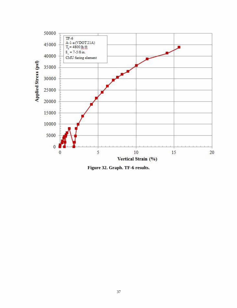
37
Figure 32. Graph. TF-6 results.

38
4.2 REPEATABILITY
The repeatability of the test method was indirectly measured through four PTs (TF-4, TF-5,
TF-7, and TF-8, see TABLE 1) on nearly identical GRS composites (figure 33). Note that TF-4
was prematurely terminated due to uneven loading and settlement and TF-8 had two courses of
bearing bed reinforcement at the top. For TF-5, the stress-strain curve for both the initial loading
sequence is plotted to compare to the other tests at lower applied loads, with the stress-strain
curve starting on the second reload cycle also plotted to compare to the other tests at higher
applied loads. All of the tests were performed without CMU facing. The results indicate good
agreement and suggest that the performance test produces repeatable results.
4.3 COMPOSITE BEHAVIOR
The new internal stability design method proposed by Adams et al. 2011a for GRS accounts for
functions of the geosynthetic reinforcement beyond simple tensile inclusions and takes into
account the backfill and reinforcement spacing comprising the GRS composite material.(1)
In this
model, connection, reinforcement pullout, and other mechanisms associated with a tie-back
design model are not modes of failures for closely spaced GRS.(10)
Adding to the understanding
of the composite behavior, conducting PTs without a CMU facing allowed for the failure surface
for each GRS composite to be visually observed.
For the PTs with reinforcement spacing less than 12 inches, a shear surface formed through the
composite (figure 34, figure 35, and figure 36), leading to rupture of the reinforcement. The
same mode of failure was not seen for the 15¼-inch spaced system (figure 37) where failure was
determined by the soil between the sheets of geotextile, and the full strength of the reinforcement
was never developed.

39
Figure 33. Graph. Repeatability of PT at TFHRC.
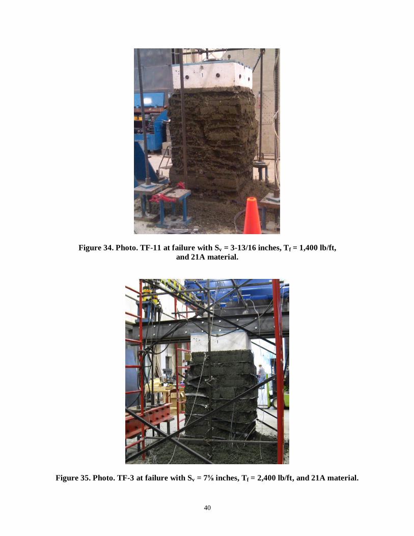
40
Figure 34. Photo. TF-11 at failure with Sv = 3-13/16 inches, Tf = 1,400 lb/ft,
and 21A material.
Figure 35. Photo. TF-3 at failure with Sv = 7⅝ inches, Tf = 2,400 lb/ft, and 21A material.

41
Figure 36. Photo. TF-13 at failure with Sv = 11¼ inches, Tf = 3,600 lb/ft, and 21A material.
Figure 37. Photo. TF-10 at failure with Sv = 15¼ inches, Tf = 4,800 lb/ft, and 21A material.
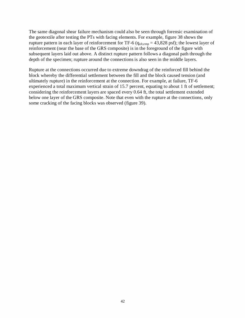
42
The same diagonal shear failure mechanism could also be seen through forensic examination of
the geotextile after testing the PTs with facing elements. For example, figure 38 shows the
rupture pattern in each layer of reinforcement for TF-6 (qult,emp = 43,828 psf); the lowest layer of
reinforcement (near the base of the GRS composite) is in the foreground of the figure with
subsequent layers laid out above. A distinct rupture pattern follows a diagonal path through the
depth of the specimen; rupture around the connections is also seen in the middle layers.
Rupture at the connections occurred due to extreme downdrag of the reinforced fill behind the
block whereby the differential settlement between the fill and the block caused tension (and
ultimately rupture) in the reinforcement at the connection. For example, at failure, TF-6
experienced a total maximum vertical strain of 15.7 percent, equating to about 1 ft of settlement;
considering the reinforcement layers are spaced every 0.64 ft, the total settlement extended
below one layer of the GRS composite. Note that even with the rupture at the connections, only
some cracking of the facing blocks was observed (figure 39).

43
Figure 38. Photo. Rupture pattern for geotextiles in TF-6 (qult,emp = 43,828 psf); the lowest
layer of reinforcement is the closet fabric in the picture.

44
Figure 39. Photo. Post-test picture of TF-6 (Sv = 7⅝ inches, Tf = 4,800 lb/ft).
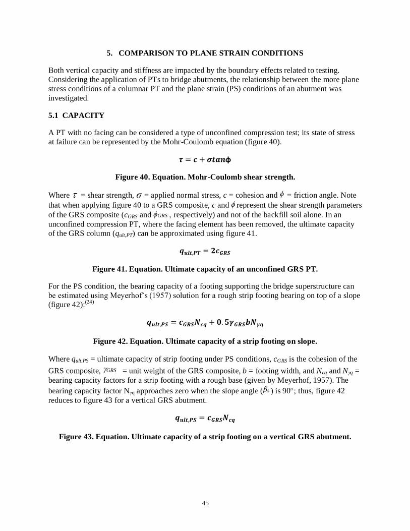
45
5. COMPARISON TO PLANE STRAIN CONDITIONS
Both vertical capacity and stiffness are impacted by the boundary effects related to testing.
Considering the application of PTs to bridge abutments, the relationship between the more plane
stress conditions of a columnar PT and the plane strain (PS) conditions of an abutment was
investigated.
5.1 CAPACITY
A PT with no facing can be considered a type of unconfined compression test; its state of stress
at failure can be represented by the Mohr-Coulomb equation (figure 40).
Figure 40. Equation. Mohr-Coulomb shear strength.
Where = shear strength, = applied normal stress, c = cohesion and = friction angle. Note
that when applying figure 40 to a GRS composite, c and represent the shear strength parameters
of the GRS composite (cGRS and respectively) and not of the backfill soil alone. In an
unconfined compression PT, where the facing element has been removed, the ultimate capacity
of the GRS column (qult,PT) can be approximated using figure 41.
Figure 41. Equation. Ultimate capacity of an unconfined GRS PT.
For the PS condition, the bearing capacity of a footing supporting the bridge superstructure can
be estimated using Meyerhof’s (1957) solution for a rough strip footing bearing on top of a slope
(figure 42):(24)
Figure 42. Equation. Ultimate capacity of a strip footing on slope.
Where qult,PS = ultimate capacity of strip footing under PS conditions, cGRSis the cohesion of the
GRS composite, = unit weight of the GRS composite, b = footing width, and Ncq and Nq =
bearing capacity factors for a strip footing with a rough base (given by Meyerhof, 1957). The
bearing capacity factor Nq approaches zero when the slope angle ( ) is 90; thus, figure 42
reduces to figure 43 for a vertical GRS abutment.
Figure 43. Equation. Ultimate capacity of a strip footing on a vertical GRS abutment.
𝝉 = 𝒄 + 𝝈𝒕𝒂𝒏φ
σ ϕ
ϕ
ϕGRS
𝒒𝒖𝒍𝒕,𝑷𝑻 = 𝟐𝒄𝑮𝑹𝑺
𝒒𝒖𝒍𝒕,𝑷𝑺 = 𝒄𝑮𝑹𝑺𝑵𝒄𝒒 + 𝟎. 𝟓𝜸𝑮𝑹𝑺𝒃𝑵𝜸𝒒
GRS
βs
𝒒𝒖𝒍𝒕,𝑷𝑺 = 𝒄𝑮𝑹𝑺𝑵𝒄𝒒
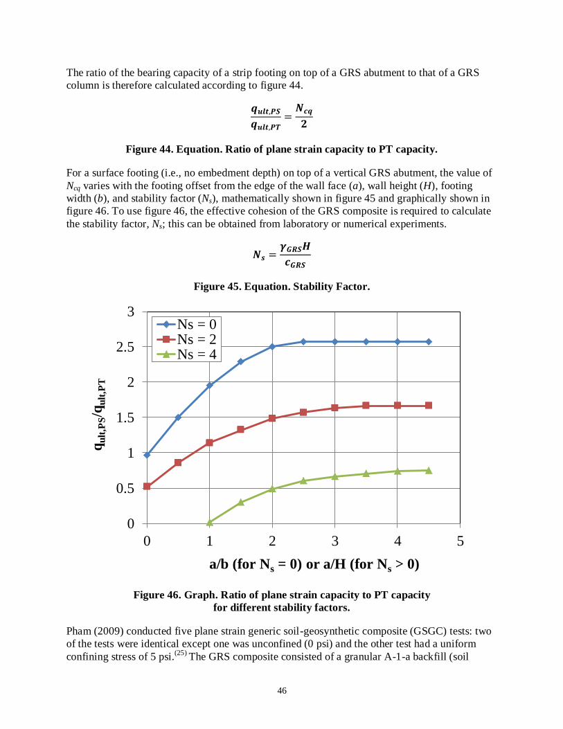
46
The ratio of the bearing capacity of a strip footing on top of a GRS abutment to that of a GRS
column is therefore calculated according to figure 44.
Figure 44. Equation. Ratio of plane strain capacity to PT capacity.
For a surface footing (i.e., no embedment depth) on top of a vertical GRS abutment, the value of
Ncq varies with the footing offset from the edge of the wall face (a), wall height (H), footing
width (b), and stability factor (Ns), mathematically shown in figure 45 and graphically shown in
figure 46. To use figure 46, the effective cohesion of the GRS composite is required to calculate
the stability factor, Ns; this can be obtained from laboratory or numerical experiments.
Figure 45. Equation. Stability Factor.
Figure 46. Graph. Ratio of plane strain capacity to PT capacity
for different stability factors.
Pham (2009) conducted five plane strain generic soil-geosynthetic composite (GSGC) tests: two
of the tests were identical except one was unconfined (0 psi) and the other test had a uniform
confining stress of 5 psi.(25)
The GRS composite consisted of a granular A-1-a backfill (soil
𝒒𝒖𝒍𝒕,𝑷𝑺
𝒒𝒖𝒍𝒕,𝑷𝑻=
𝑵𝒄𝒒
𝟐
𝑵𝒔 =𝜸𝑮𝑹𝑺𝑯
𝒄𝑮𝑹𝑺
0
0.5
1
1.5
2
2.5
3
0 1 2 3 4 5
qu
lt,P
S/q
ult
,PT
a/b (for Ns = 0) or a/H (for Ns > 0)
Ns = 0Ns = 2Ns = 4

47
classification = GW-GM, unit weight, = 153.7 lb/ft3, cohesion, c = 1,480 psf and friction
angle, = 50º) and a 4,800 lb/ft geotextile reinforcement spaced at 7⅝ inches. The corresponding
failure stresses were about 42,450 psf and 70,957 psf for the 0 and 5 psi confining stresses,
respectively. These failure stresses are calculated as the ratio of applied vertical load to the area
of the top load pad (i.e. footing) on the GSGC mass for each test. Note that Pham (2009)
reported failure stresses as the ratio of applied vertical load to the total area of the GSGC
mass.(25)
The results of these tests can be used to determine the strength properties (cohesion and friction
angle) of a particular GRS composite. The Mohr-Coulomb failure circles for the two Pham
(2009) tests are shown in figure 47; the resulting cohesion and friction angle for the GRS
composite tested is 3,342 psf and 72º, respectively; the stability factor (figure 45) is 0.29. Based
on this stability factor, the ratio of plane strain capacity to column (PT) capacity varies with a/H
(figure 48). The correction factor to convert from the PT to a plane strain condition for a typical
GRS abutment with the setback (a) equal to 8 inches and height from 10 to 30 ft (i.e., a/H = 0.02
to 0.07) ranges between 0.92 and 0.97 for this particular GRS composite, close to unity.
Therefore, the failure of the PT is approximately representative of an in-service PS condition for
well-graded gravels, meaning the PT results can be directly used to estimate the strength limit for
capacity in design. Note that the strength properties of the foundation soil underneath in-service
GRS abutments would still need to be verified separately.(1)
Note that there are some limitations to the formulation above. The relationship between the
bearing capacity of the strip footing and the performance tests requires the cohesion and friction
angle of the GRS composite, which are not easy parameters to determine. Additional work is
required to develop relationships between the composite shear strength parameters and the soil
shear strength parameters, with respect to reinforcement spacing and strengths.
Figure 47. Graph. Mohr-Coulomb failure envelope for Pham (2009)
plane strain GSGC tests.
γ
ϕ
0
10000
20000
30000
40000
50000
60000
70000
80000
0 20000 40000 60000 80000
Sh
ea
r S
tress
(p
sf)
Normal Stress (psf)
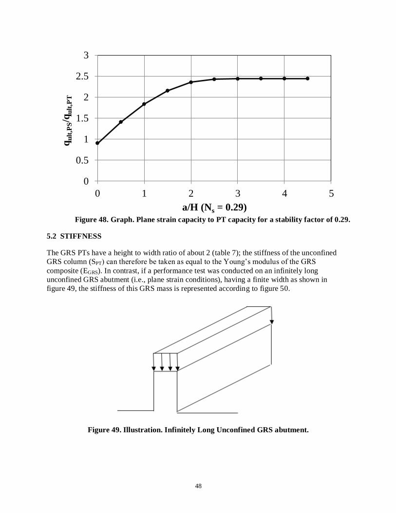
48
Figure 48. Graph. Plane strain capacity to PT capacity for a stability factor of 0.29.
5.2 STIFFNESS
The GRS PTs have a height to width ratio of about 2 (table 7); the stiffness of the unconfined
GRS column (SPT) can therefore be taken as equal to the Young’s modulus of the GRS
composite (EGRS). In contrast, if a performance test was conducted on an infinitely long
unconfined GRS abutment (i.e., plane strain conditions), having a finite width as shown in
figure 49, the stiffness of this GRS mass is represented according to figure 50.
Figure 49. Illustration. Infinitely Long Unconfined GRS abutment.
0
0.5
1
1.5
2
2.5
3
0 1 2 3 4 5
qu
lt,P
S/q
ult
,PT
a/H (Ns = 0.29)

49
Figure 50. Equation. Stiffness of an Infinitely Long Unconfined GRS abutment.
Where q = applied stress, = vertical strain, EGRS = Young’s modulus of the GRS and =
Poisson’s ratio of the GRS. Assuming is equal to 0.5, this infinitely long GRS strip will be
1.33 times stiffer than a square GRS column.(2)
In reality, the width is not finite in the direction
perpendicular to a GRS abutment, as shown on the left of figure 51. To date, typical L/b ratios
for in-service GRS abutments range between 7 and 14, depending on load requirements, where L
is the length and b is the width of the bearing area. NAVFAC (1986) considers L/b ratios > 5 to
be plane strain while current FHWA practice considers L/b ratios > 10 to be plane strain
conditions; therefore, most GRS abutments can be idealized as plane strain.(26)
In the context of elastic theory, the bridge footing on a GRS abutment can be considered a strip
running parallel to the edge of the wall at an offset, as shown on the left side of figure 51.
Considering the response at low strain levels is close to elastic conditions, the stiffness of such a
strip surface footing can be estimated using elastic theory, in particular the solution for a strip
footing on a linear elastic half space.(27,28)
Since the conditions are not a linear elastic half space
for abutment applications, the solution for a strip footing on top of a wall is obtained by doubling
the solution for a strip footing on a linear elastic half space, as shown on the right side of
figure 51. Note that this assumes zero lateral deformations along the wall height, which is not
strictly correct for GRS abutments since the CMU facing is free to displace laterally; however, it
is the best available method to date to estimate vertical settlement.
Figure 51. Illustration. Solution for strip footing on top of a wall.
For a material with a Poisson’s ratio of 0.5, Gibson (1967) provided solutions for the relative
displacement between the center of the strip footing and any arbitrary point assuming a constant
stiffness with depth.(27)
If the arbitrary point is selected to be the bottom of the GRS wall, the
expression for settlement without doubling the load is shown in figure 52.
𝒒
𝜺𝒗=
𝐄𝐆𝐑𝐒
(𝟏 + 𝑽𝑮𝑹𝑺)(𝟏 − 𝑽𝑮𝑹𝑺)
v GRS
GRS

50
Figure 52. Equation. Vertical displacement of a GRS abutment with a strip footing.
Where q = applied stress, b is the footing width, EGRS is the Young’ modulus of the GRS
composite, a is the setback distance between the face of the wall and the applied load, and H is
the height of the abutment. The corresponding vertical strain ( ) is given by figure 53.
Figure 53. Equation. Vertical strain.
Where is the vertical displacement (figure 52) and H is the height of the wall.
The stiffness of a GRS abutment supporting a surface strip footing (SGRS) can be related to the
applied stress (2q, due to doubling of the load) and the vertical strain ( ) (figure 54).
Figure 54. Equation. Stiffness of a GRS abutment supporting a strip footing.
The ratio between this stiffness and the stiffness from a performance test (SGRS = EGRS) can then
be calculated according to figure 55. The variation of stiffness ratio with b/H is plotted in
figure 56. It was found that this ratio is essentially independent of the value of a/b.
Figure 55. Equation. Vertical displacement of a GRS abutment with a strip footing.
𝝆 =𝟑𝒒𝒃
𝟒𝝅𝑬𝑮𝑹𝑺 𝟏
𝟐 𝟏 +
𝒂 +𝒃𝟐
𝒃𝟐
𝒍𝒏 𝑯𝟐 + (𝒂 +
𝒃𝟐)𝟐
(𝒃𝟐
)𝟐 +
𝟏
𝟐 𝟏 −
𝒂 +𝒃𝟐
𝒃𝟐
𝒍𝒏 𝑯𝟐 + 𝒂𝟐
(𝒃𝟐
)𝟐
+𝑯
𝒂𝒕𝒂𝒏−𝟏
𝒂 + 𝒃
𝑯 +
𝑯
𝒂𝒕𝒂𝒏−𝟏
−𝒃
𝑯
v
𝜺𝒗 =𝝆
𝑯
ρ
v
𝑺𝑮𝑹𝑺 =𝟐𝒒
𝜺𝒗=
𝟐𝒒𝑯
𝝆
𝑺𝑮𝑹𝑺
𝑺𝑷𝑻
=𝟐𝒒𝑯𝝆𝑬𝑮𝑹𝑺
= 𝟖𝝅𝑯
𝟑𝒃 𝟏𝟐 𝟏 +
𝒂 +𝒃𝟐
𝒃𝟐
𝒍𝒏 𝑯𝟐 + (𝒂 +
𝒃𝟐)𝟐
(𝒃𝟐
)𝟐 +
𝟏𝟐 𝟏 −
𝒂 +𝒃𝟐
𝒃𝟐
𝒍𝒏 𝑯𝟐 + 𝒂𝟐
(𝒃𝟐
)𝟐 +
𝑯𝒂
𝒕𝒂𝒏−𝟏 𝒂 + 𝒃
𝑯 +
𝑯𝒂
𝒕𝒂𝒏−𝟏 −𝒃𝑯

51
Figure 56. Graph. Ratio of plane strain stiffness of a strip footing on top of a wall (SGRS) to
that of a PT (SPT) for the case of constant stiffness with depth.
For GRS abutments, b is a minimum of 2.5 ft for bridge spans larger than 25 ft and has been as
large as 4.5 ft for the Tiffin River Bridge; H typically ranges from 10 to 30 ft; b/H is therefore
between about 0.08 and 0.45.(5)
From figure 56, the ratio of plane strain stiffness of a strip
footing on top of a wall (SGRS) to that of a PT (SPT) ranges between 0.92 and 3 suggesting that the
stiffness reported from a PT will be conservative (up to a factor of three times) compared to what
a GRS abutment might experience in-service.
Note that further research should be conducted on the stiffness of GRS abutments, and the
corresponding equivalency to a GRS PT, since the above formulations are simplistic and do not
consider the effects of the facing element (e.g., CMUs) on the capacity and stiffness of a GRS
composite. The effect of compaction-induced stresses and related shakedown is also ignored.
Compaction-induced stresses increase the locked-in lateral stress especially in the upper reaches
of the GRS; associated with an increase in confinement is an increase in stiffness and its effects
should be investigated.
0
0.5
1
1.5
2
2.5
3
3.5
4
0 0.1 0.2 0.3 0.4 0.5 0.6 0.7
S GR
S/
S PT
b/H


53
6. PARAMETRIC ANALYSIS
The combined series of tests performed in Defiance County and at TFHRC make up a parametric
study where the following parameters were investigated: (1) aggregate type, (2) compaction,
(3) gradation, (4) bearing bed reinforcement, (5) reinforcement strength, (6) similar ratios of
reinforcement strength to spacing, (Tf/Sv), and (7) facing.
6.1 EFFECT OF AGGREGATE TYPE
The aggregate selected has a large impact on the performance and composite behavior of GRS;
both the size (i.e., dmax) and the strength (i.e., c, ) of the backfill selected are important. In PTs,
it is very difficult to isolate one backfill variable over another to determine the individual
contributions to GRS performance. Instead, general conclusions based on aggregate
classification and angularity can be drawn using PT results; however, advanced computer
modeling is a potential avenue to better understand the component contributions of particular fill
materials.
The majority of GRS- Integrated bridge systems (IBSs) built across the country use an open-
graded aggregate for the abutment backfill. Commonly, an AASHTO No. 89 has been employed;
an early performance test performed in Defiance County shows the behavior of a GRS composite
with this backfill and 4,800 lb/ft reinforcement spaced at 7⅝ inches.(1)
To create a database of
PT results with alternate aggregate types, while providing an opportunity to demonstrate the
construction of a PT to FHWA Division Offices, Federal Lands Highway Division, and the
Resource Center through the EDC GRS-IBS Validation Sessions, a series of tests were
conducted in this study (table 9). Note that since these PTs were conducted as demonstration
piers, the level of compaction control on each lift was not consistent or uniform.
Table 9. Parametric study on aggregate size.
Test
No.
Backfill Reinforcement
Facing Type
(°)
c
(psf)
dmax
(inch)
Tf
(lb/ft)
Sv
(in.)
DC-1 8 54 0 ½ 4,800 7⅝** CMU
DC-2 8P* 46 0 ¾ 4,800 7⅝** CMU
DC-3 57 52 0 1 4,800 7⅝** CMU
DC-4 9 49 0 ⅜ 4,800 7⅝** CMU
ϕ = the peak friction angle, c = the cohesion, Tf = the MARV value of the wide width tensile
strength, and Sv = the spacing.
*Rounded pea-gravel angularity.
**Two courses of bearing bed reinforcement placed at the top of the PT.
Based on the results (table 10), no relationship can be determined with respect to the strength
limit for open-graded aggregates since there are only two PTs conducted to failure of the GRS
composite. The largest aggregate tested, the No. 57 stone, had the lowest service limit of all the
tests, indicating more deformation under an applied load. In addition, the rounded pea gravel had
a lower strength and service limit than the more angular aggregate meeting the same gradation
specifications for an AASHTO No. 8 material.
ϕ
ϕ

54
Table 10. Effect of aggregate type results.
Maximum Tested
Strength
Limit Design Limit
Service
Limit
Test
No.
qmax
(psf) (%)
qult,emp
(psf)
(psf)
Vallow =
/3.5 (psf)
(psf)
DC-1 23,310 7.95 23,310 19,983 5,709 3,065
DC-2 22,709 7.07 22,709 19,399 5,543 2,171
DC-3 18,447 5.82 N/A 16,182 4,623 1,324
DC-4 26,730 7.64 N/A 17,350 4,957 2,212
qmax = the maximum applied pressure during testing, = the maximum recorded
vertical strain, qult,emp = the measured failure pressure, = the applied stress at
5-percent vertical strain, Vallow,emp = the total allowable pressure on the GRS,(1)
= the applied stress at 0.5-percent vertical strain.
6.2 EFFECT OF COMPACTION
The effect of compaction for open-graded materials was investigated through two PTs conducted
in Defiance County, OH (table 11). The testing conditions were identical except for the
compaction effort. DC-1 was compacted to non-movement while DC-5 involved no compaction
effort beyond end dumping the material and leveling for each lift of fill. The results show a
similar vertical capacity (23,310 psf versus 21,539 psf for DC-1 and DC-5, respectively);
however, the higher strength for DC-1 is likely due to the increased locked-in stresses induced
due to compaction. Note that the friction angle of both composites is reported as the same;
however, the degree of compaction may have a small impact for open-graded aggregates (larger
for well-graded backfills). This effect is currently being investigated.
While the capacity of the specimens was similar, the deformation response was different
(figure 57). As expected, Test DC-5 had a softer response resulting from not being compacted.
The modulus of the primary settlement portion of the curve for the uncompacted composite
(DC-5) is about 270 ksf while the modulus for the compacted composite (DC-1) is 430 ksf
(table 11).
εmax q@ε≤5% q@ε≤5% q@ε=0.5%
εmax q@ε=5%
q@ε=0.5%

55
Table 11. Parametric study on compaction.
Test
No.
Backfill Reinforcement
Facing
Eo
(ksf)
qult,emp
(psf) Type
(°)
c
(psf)
Tf
(lb/ft)
Sv
(in.)
DC-1 8 54 0 4,800 7⅝** CMU 430 23,310
DC-5 8*** 54 0 4,800 7⅝** CMU 270 21,539
= the peak friction angle, c = the cohesion, Tf = the MARV value of the wide width tensile
strength, Sv = the spacing, Eo = the initial stress-strain ratio, and qult,emp = the measured vertical
capacity.
**Two courses of bearing bed reinforcement placed at the top of the PT.
***Uncompacted sample.
At the service limit state of 0.5 percent vertical strain, the allowable stress is limited to 316 psf
for the uncompacted GRS composite, but 3,065 psf for the same composite compacted to non-
movement (table 8); however, if negating the initial immediate settlement resulting from the first
load increment, before the onset of primary deformation of the uncompacted sample, the
allowable stress is about 1,345 psf (figure 58).
The ratio of strain for the uncompacted (DC-5) and compacted (DC-1) GRS composite
( / ), accounting for the immediate deformation related to the uncompacted
composite (DC-5), decreases with increasing applied pressure (figure 59). For the particular GRS
composite tested (table 11, figure 58), at an in-service dead load of 4,000 psf, an uncompacted
abutment will experience about 3 times the strain as a compacted abutment; however, near
failure, at about 20,000 psf, an uncompacted abutment will experience about 1.7 times the strain
as a compacted abutment. Note that in the evaluation of tolerable settlements for highway bridge
design, FHWA recommends the construction-point concept, whereby the settlements between
critical construction points (such as between application of dead load and opening to traffic) are
evaluated.(29)
ϕ
ϕ
εv,uncompact εv,compact

56
Figure 57. Graph. Comparison between compacted and uncompacted GRS composites.

57
Figure 58. Design service limit for uncompacted sample DC-5.
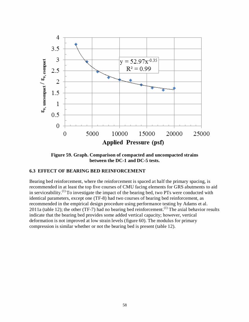
58
Figure 59. Graph. Comparison of compacted and uncompacted strains
between the DC-1 and DC-5 tests.
6.3 EFFECT OF BEARING BED REINFORCEMENT
Bearing bed reinforcement, where the reinforcement is spaced at half the primary spacing, is
recommended in at least the top five courses of CMU facing elements for GRS abutments to aid
in serviceability.(1)
To investigate the impact of the bearing bed, two PTs were conducted with
identical parameters, except one (TF-8) had two courses of bearing bed reinforcement, as
recommended in the empirical design procedure using performance testing by Adams et al.
2011a (table 12); the other (TF-7) had no bearing bed reinforcement.(1)
The axial behavior results
indicate that the bearing bed provides some added vertical capacity; however, vertical
deformation is not improved at low strain levels (figure 60). The modulus for primary
compression is similar whether or not the bearing bed is present (table 12).

59
Table 12. Parametric study on bearing bed reinforcement.
Test
No.
Backfill Reinforcement
Facing
Eo
(ksf)
qult,emp
(psf) Type (°)
c
(psf)
dmax
(in.)
Tf
(lb/ft)
Sv
(in.)
TF-7 21A 53 115 1 4,800 7⅝ no CMU 320 26,546
TF-8 21A 53 115 1 4,800 7⅝** no CMU 320 29,134
= the peak friction angle, c = the cohesion, Tf = the MARV value of the wide width tensile
strength, Sv = the spacing, Eo = the initial stress-strain ratio, and qult,emp = the measured vertical
capacity.
**Two courses of bearing bed reinforcement placed at the top of the PT.
Figure 60. Graph. Effect of bearing bed reinforcement for TF-7 and TF-8.
Looking at the lateral deformation characteristics for both tests at an applied stress of about
3,600 psf, typical of bridge loads (figure 61), the bearing bed reinforcement serves to limit
deformation in the zone of its placement. The approximate location of the bearing bed
reinforcement is illustrated with red dashed lines in figure 61. At considerably higher loads,
around 26,600 psf, the same effect is observed (figure 62). Note that the LVDT located at the
bottom of the PT for the TF-7 test was damaged during testing due to sloughing of the fill
ϕ
ϕ
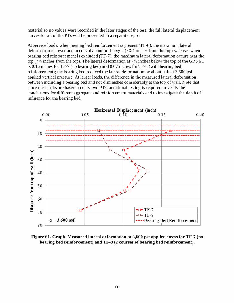
60
material so no values were recorded in the later stages of the test; the full lateral displacement
curves for all of the PTs will be presented in a separate report.
At service loads, when bearing bed reinforcement is present (TF-8), the maximum lateral
deformation is lower and occurs at about mid-height (38⅛ inches from the top) whereas when
bearing bed reinforcement is excluded (TF-7), the maximum lateral deformation occurs near the
top (7⅝ inches from the top). The lateral deformation at 7⅝ inches below the top of the GRS PT
is 0.16 inches for TF-7 (no bearing bed) and 0.07 inches for TF-8 (with bearing bed
reinforcement); the bearing bed reduced the lateral deformation by about half at 3,600 psf
applied vertical pressure. At larger loads, the difference in the measured lateral deformation
between including a bearing bed and not diminishes considerably at the top of wall. Note that
since the results are based on only two PTs, additional testing is required to verify the
conclusions for different aggregate and reinforcement materials and to investigate the depth of
influence for the bearing bed.
Figure 61. Graph. Measured lateral deformation at 3,600 psf applied stress for TF-7 (no
bearing bed reinforcement) and TF-8 (2 courses of bearing bed reinforcement).

61
Figure 62. Graph. Measured lateral deformation at 26,600 psf applied stress for TF-7 (no
bearing bed reinforcement) and TF-8 (2 courses of bearing bed reinforcement).
6.4 Effect of Gradation
For the GRS-IBS, both open-graded and well-graded materials that meet the specifications in the
Interim Implementation Guide are acceptable for use in the GRS abutment; however, there are
advantages and disadvantages of both.(1)
Open-graded materials are free draining, easier to work
with, and their use in construction is independent of weather conditions; however, they are less
stiff than well-graded materials, which can achieve greater density under the same compactive
effort. In addition, the classical bell-shaped Proctor curves cannot be attained with open-graded
materials. The primary disadvantage of working with well-graded fill is compaction control and
maintaining the optimum moisture content for efficient compaction.
PTs TF-1 and TF-2 are identical except for the backfill material type; TF-1 used an open-graded
AASHTO No. 8 while TF-2 used a well-graded AASHTO A-1-a backfill (table 13). The friction
angle for both tests were similar (55° versus 53° for TF-1 and TF-2, respectively), but the well-
graded material (TF-2) had cohesion of 115 psf. The corresponding soil shear strengths at a
given applied stress (figure 40) are therefore only 5 percent different, with TF-2 having slightly
higher shear strength.

62
Table 13. Parametric study on gradation (Tf = 2,400 lb/ft, Sv = 7⅝ inches).
Test
No.
Backfill Reinforcement
Facing
Eo
(ksf)
qult,emp
(psf) Type (°)
c
(psf)
dmax
(inch)
Tf
(lb/ft)
Sv
(inch)
TF-1++
8 55 0 ½ 2,400 7⅝ CMU 320 20,487
TF-2 21A 53 115 1 2,400 7⅝ CMU 710 25,260
= the peak friction angle, c = the cohesion, Tf = the MARV value of the wide width tensile
strength, Sv = the spacing, Eo = the initial stress-strain ratio, and qult,emp = the measured vertical
capacity.
++Technical difficulties resulted in unloading/reloading of the composite.
The resulting load-deformation profiles are shown in figure 63. The well-graded material is
considerably stiffer than the open-graded material. At an applied pressure of 4,000 psf, the
vertical strain is about 1.1 percent for TF-1 (open-graded) and 0.4 percent for TF-2 (well-
graded). The modulus of the composite tested in TF-1 is 320 ksf (table 13) compared to 710 ksf
for the composite tested in TF-2; TF-1 (open-graded) is 55 percent less stiff than TF-2 (well-
graded). In terms of bearing capacity, TF-1 was 20 percent less strong than TF-2. The results
indicate that the gradation, and perhaps cohesion, impacts the stiffness more so than strength,
indicating that well-graded fills have an advantage with respect to serviceability. As previously
discussed in section 6.1, isolating the effect of cohesion on the performance is difficult using
PTs, although based on the soil-geosynthetic capacity equation (figure 8), it will serve to
improve capacity, although its contribution should not be considered in design.
ϕ
ϕ

63
Figure 63. Graph. Comparison of open-graded and well-graded backfills
for TF-1 and TF-2.
Comparing DC-1 and TF-6 also provides similar insight into the modulus difference between
open-graded and well-graded composites, respectively (table 14). Note that DC-1 included two
courses of bearing bed reinforcement; however, it was previously shown that the bearing bed
reinforcement does not impact the modulus at low strain levels, but the capacity is slightly
improved with the two additional layers of reinforcement at the top. The modulus of the
composite with open-graded backfill (DC-1) was 430 ksf, whereas the modulus of the composite
with well-graded backfill (TF-6) was 750 ksf. Both are slightly larger than the measured
modulus of similar composites with lower reinforcement strengths (table 13).

64
Table 14. Parametric study on gradation (Tf = 4,800 lb/ft, Sv = 7⅝ inches.)
Test
No.
Backfill Reinforcement
Facing
Eo
(ksf)
qult,emp
(psf) Type (°)
c
(psf)
dmax
(inch)
Tf
(lb/ft)
Sv
(inch)
DC-1 8 54 0 ½ 4,800 7⅝** CMU 430 23,310
TF-6++
21A 53 115 1 4,800 7⅝ CMU 750 43,763
ϕ = the peak friction angle, c = the cohesion, Tf = the MARV value of the wide width tensile
strength, Sv = the spacing, Eo = the initial stress-strain ratio, and qult,emp = the measured vertical
capacity.
**Two courses of bearing bed reinforcement placed at the top of the PT.
++Technical difficulties resulted in unloading/reloading of the composite.
6.5 EFFECT OF REINFORCEMENT STRENGTH
The impact of reinforcement strength on the behavior of a GRS composite was investigated for
both open-graded (table 15) and well-graded aggregates (table 16).
Table 15. Parametric study on reinforcement strength with open-graded aggregates.
Test
No.
Backfill Reinforcement
Facing
Eo
(ksf)
qult,emp
(psf) Type
(°)
c
(psf)
dmax
(inch)
Tf
(lb/ft)
Sv
(inch)
DC-1 8 54 0 ½ 4,800 7⅝** CMU 430 23,310
TF-1++
8 55 0 ½ 2,400 7⅝ CMU 320 20,487
ϕ = the peak friction angle, c = the cohesion, Tf = the MARV value of the wide width tensile
strength, Sv = the spacing, Eo = the initial stress-strain ratio, and qult,emp = the measured vertical
capacity.
**Two courses of bearing bed reinforcement placed at the top of the PT.
++Technical difficulties resulted in unloading/reloading of the composite.
Table 16. Parametric study on reinforcement strength with well-graded aggregates.
Test
No.
Backfill Reinforcement
Facing
Eo
(ksf)
qult,emp
(psf) Type
(°)
c
(psf)
dmax
(inch)
Tf
(lb/ft)
Sv
(inch)
TF-2 21A 53 115 1 2,400 7⅝ CMU 710 25,260
TF-6++
21A 53 115 1 4,800 7⅝ CMU 750 43,763
= the peak friction angle, c = the cohesion, Tf = the MARV value of the wide width tensile
strength, Sv = the spacing, Eo = the initial stress-strain ratio, and qult,emp = the measured vertical
capacity.
++Technical difficulties resulted in unloading/reloading of the composite.
DC-1 and TF-1 both tested similar open-graded aggregates (AASTHO No. 8s) at the same
reinforcement spacing of 7⅝ inches, but DC-1 used a 4,800 lb/ft geotextile while TF-1 used a
2,400 lb/ft geotextile (table 15). The response indicates that the higher reinforcement strength
ϕ
ϕ
ϕ
ϕ

65
(4,800 lb/ft) produces a stiffer and stronger response than the lower reinforcement strength
(2,400 lb/ft) for open-graded backfill. By doubling the reinforcement strength, the results
indicate an increase by a factor of 1.14 for capacity and 1.34 for the initial stress-strain ratio.
Comparing the effect of reinforcement strength with a well-graded AASHTO A-1-a aggregate,
with and without facing, it was found that increasing the ultimate reinforcement strength
(MARV) by a factor of two from 2,400 lb/ft (TF-2) to 4,800 lb/ft (TF-6) at the same
reinforcement spacing (Sv = 7⅝ inches) results in an increase in the measured capacity and initial
stress-strain ratio by a factor of 1.73 and 1.06, respectively for CMU facing (table 16). When no
facing is present, the same increase in reinforcement strength from 2,400 lb/ft (TF-3) to
4,800 lb/ft (TF-7) at a spacing of 7⅝ inches results in an increase in the measured capacity by a
factor of 1.5. For open-graded aggregates, the percent increase in capacity is less than for the
well-graded material tested which may be due to the increased cohesion and maximum density of
the well-graded material, thus leading to higher soil shear strengths and increased stiffness
properties.
6.6 EFFECT OF THE RELATIONSHIP BETWEEN REINFORCEMENT STRENGTH
AND SPACING
The current AASHTO LRFD Bridge Design Specifications (2012) do not distinguish between
MSE technology and closely-spaced GRS technology.(30)
In AASHTO (2012), reinforcement
spacing is linearly proportional to the reinforcement strength, leading engineers to prefer larger
spaced systems with proportionally greater reinforcement strengths.(10)
Research on closely
spaced systems, however, indicates that reinforcement spacing plays a significantly larger role
than the reinforcement strength.(5,11 ,25 ,31)
To investigate the relationship between the MARV wide width reinforcement tensile strength
(Tf) and spacing (Sv), several PTs were designed to keep the same Tf /Sv ratios, both with
(table 17) and without facing elements (table 18). The strength of the reinforcement was assumed
to be the manufacturer supplied MARV (table 6). Within the data set of this study, there are three
pairs of tests (with and without facing) at a constant Tf /Sv ratio (table 19). For a Tf /Sv ratio of
3,800 lb/ft2, the load-test curves for the tests with facing are presented in figure 64 and the load-
test curves for the tests without facing are presented in figure 65.
Table 17. Parametric study for 3,800 lb/ft2 Tf/Sv ratio (with facing).
Test
No.
Backfill Reinforcement
Facing
Eo
(ksf)
qult,emp
(psf) Type
(°)
c
(psf)
dmax
(in.)
Tf
(lb/ft)
Sv
(in.)
TF-2 21A 53 115 1 2,400 7⅝ CMU 710 25,260
TF-9 21A 53 115 1 4,800 15¼ CMU 550 22,310
TF-14 21A 53 115 1 3,600 11¼ CMU 460 23,562
= the peak friction angle, c = the cohesion, Tf = the MARV value of the wide width tensile
strength, Sv = the spacing, Eo = the initial stress-strain ratio, and qult,emp = the measured vertical
capacity.
ϕ
ϕ
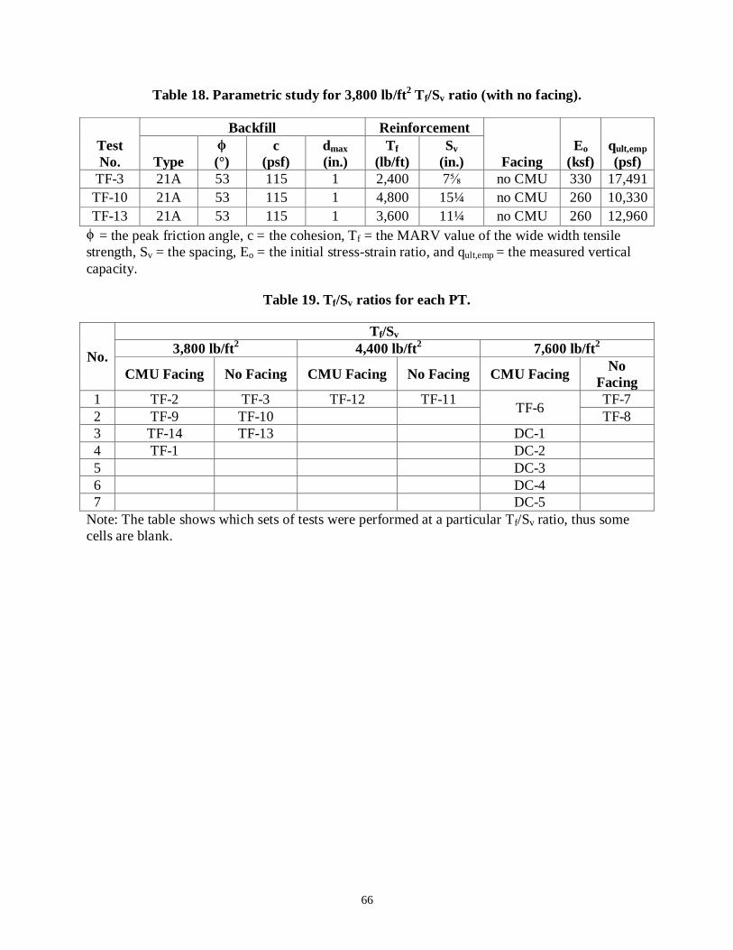
66
Table 18. Parametric study for 3,800 lb/ft2 Tf/Sv ratio (with no facing).
Test
No.
Backfill Reinforcement
Facing
Eo
(ksf)
qult,emp
(psf) Type
(°)
c
(psf)
dmax
(in.)
Tf
(lb/ft)
Sv
(in.)
TF-3 21A 53 115 1 2,400 7⅝ no CMU 330 17,491
TF-10 21A 53 115 1 4,800 15¼ no CMU 260 10,330
TF-13 21A 53 115 1 3,600 11¼ no CMU 260 12,960
= the peak friction angle, c = the cohesion, Tf = the MARV value of the wide width tensile
strength, Sv = the spacing, Eo = the initial stress-strain ratio, and qult,emp = the measured vertical
capacity.
Table 19. Tf/Sv ratios for each PT.
No.
Tf/Sv
3,800 lb/ft2 4,400 lb/ft
2 7,600 lb/ft
2
CMU Facing No Facing CMU Facing No Facing CMU Facing No
Facing
1 TF-2 TF-3 TF-12 TF-11 TF-6
TF-7
2 TF-9 TF-10 TF-8
3 TF-14 TF-13 DC-1
4 TF-1 DC-2
5 DC-3
6 DC-4
7 DC-5
Note: The table shows which sets of tests were performed at a particular Tf/Sv ratio, thus some
cells are blank.
ϕ
ϕ

67
Figure 64. Graph. Stress-strain curves for PTs with CMUs at Tf/Sv = 3,800 psf

68
Figure 65. Graph. Stress-strain curves for PTs with no CMU facing at Tf/Sv = 3,800 psf.

69
For a Tf/Sv ratio of 3,800 lb/ft2, as the reinforcement spacing increased, the vertical capacity
decreased for the same Tf/Sv ratio, whether a CMU facing was absent (figure 66) or present
(figure 67). Contrary to MSE design theory, as reinforcement strength increased, while
increasing the spacing proportionally, the vertical capacity decreased, whether a CMU facing
was absent (figure 68) or present (figure 69).
This suggests that the relationship between reinforcement strength and spacing is not
proportional to capacity as outlined in current MSE design; a GRS abutment with a given Tf and
Sv will not have the same strength figure as a GRS abutment with twice the strength (2Tf) and
reinforcement spacing (2Sv).
Figure 66. Graph. Capacity of GRS with no CMU facing at various reinforcement spacing
for different Tf/Sv ratios.
0
5000
10000
15000
20000
25000
30000
0 5 10 15 20
Verti
cal
Cap
acit
y (
psf
)
Reinforcement Spacing (inch)
Tf/Sv = 3800 psf
Tf/Sv = 4400 psf
Tf/Sv = 7600 psf
No CMU Facing

70
Figure 67. Graph. Capacity of GRS with CMU facing at various reinforcement spacing for
different Tf/Sv ratios.
Figure 68. Graph. Capacity of GRS with no CMU facing at various reinforcement strength
for different Tf/Sv ratios.
0
5000
10000
15000
20000
25000
30000
35000
40000
45000
50000
0 5 10 15 20
Verti
ca
l C
ap
acit
y (
psf
)
Reinforcement Spacing (inch)
Tf/Sv = 3800 psf
Tf/Sv = 4400 psf
Tf/Sv = 7600 psf
CMU Facing
0
5000
10000
15000
20000
25000
30000
0 2000 4000 6000
Verti
cal
Cap
acit
y (
psf
)
Reinforcement Strength (lb/ft)
Tf/Sv = 3800 psf
Tf/Sv = 4400 psf
Tf/Sv = 7600 psf
No CMU Facing

71
Figure 69. Graph. Capacity of GRS with CMU facing at various reinforcement strength for
different Tf/Sv ratios.
At the same Tf/Sv ratio of 3,800 lb/ft2, increasing the reinforcement spacing and reinforcement
strength by a factor of two from 7⅝ to 15¼ inches and 2,400 to 4,800 lb/ft, respectively, resulted
in a reduction of the capacity by a factor of 0.9 and 0.6 for CMU facing and no facing,
respectively. According to the design theory employed by AASHTO (2012), there would be no
reduction in capacity.(10)
The relationship between reinforcement strength and spacing is
therefore not directly proportional. The results are similar to those reported by Pham (2009).(25)
6.7 EFFECT OF FACING
In the GRS-IBS Interim Implementation Guide, the effect of the facing is ignored in determining
the capacity of a GRS composite (i.e., confining stress is equal to zero in figure 8).(1)
The PTs
provide insight on the magnitude of the impact CMU facing elements have on the performance
of GRS composites. Of the nineteen tests included in this study, there were five pairs of identical
GRS composites constructed with the well-graded aggregate; each pair consisted of one test with
a frictionally connected CMU facing and another test without the CMU facing (table 21). The
stress-strain response for each pair is shown in figure 70 through figure 74.
0
5000
10000
15000
20000
25000
30000
35000
40000
45000
50000
0 2000 4000 6000
Verti
ca
l C
ap
acit
y (
psf
)
Reinforcement Strength (lb/ft)
Tf/Sv = 3800 psf
Tf/Sv = 4400 psf
Tf/Sv = 7600 psf
CMU Facing
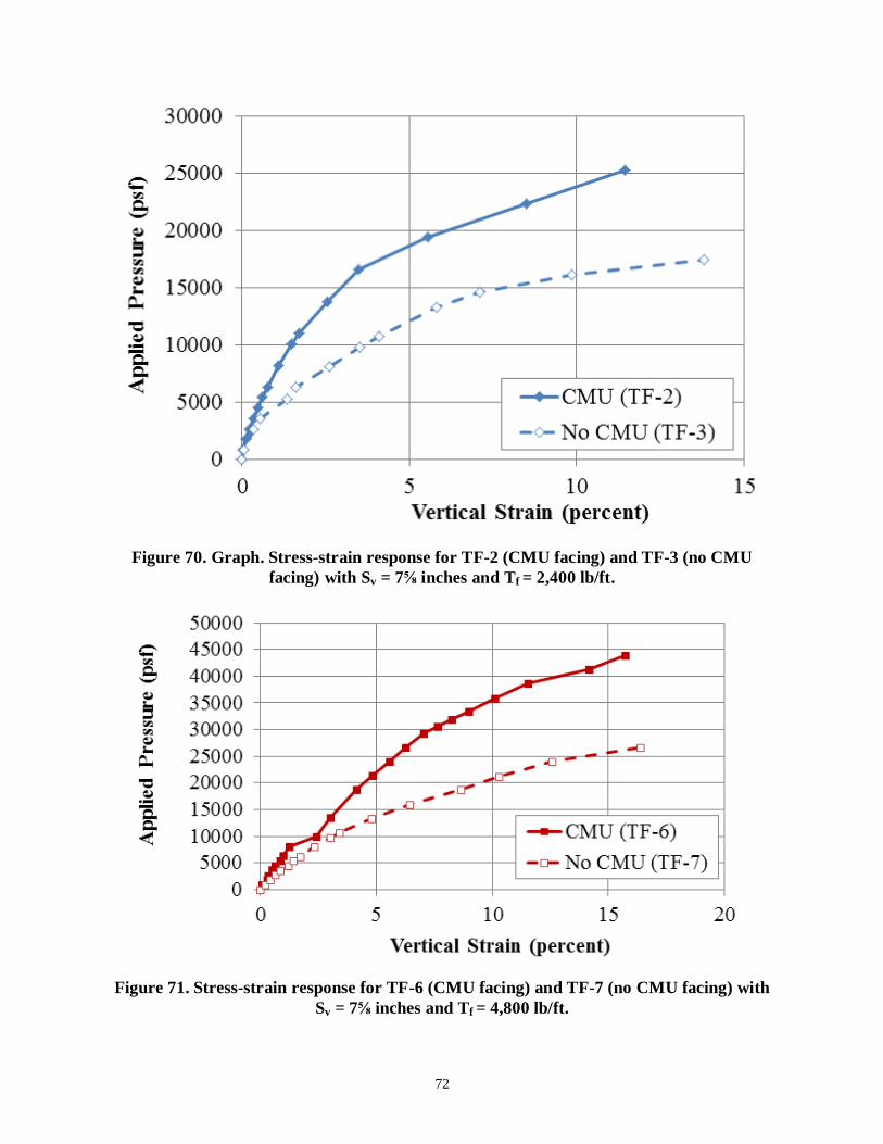
72
Figure 70. Graph. Stress-strain response for TF-2 (CMU facing) and TF-3 (no CMU
facing) with Sv = 7⅝ inches and Tf = 2,400 lb/ft.
Figure 71. Stress-strain response for TF-6 (CMU facing) and TF-7 (no CMU facing) with
Sv = 7⅝ inches and Tf = 4,800 lb/ft.

73
Figure 72. Graph. Stress-strain response for TF-9 (CMU facing) and TF-10 (No CMU
facing) with Sv = 15¼ inches and Tf = 4,800 lb/ft.

74
Figure 73. Graph. Stress-strain Response for TF-12 (CMU facing) and TF-11 (no CMU
facing) with Sv = 3-13/16 inches and Tf = 1,400 lb/ft.
Figure 74. Graph. Stress-strain response for TF-14 (CMU facing) and TF-13 (no CMU
facing) with Sv = 11¼ inches and Tf = 3,600 lb/ft.

75
The frictionally connected CMU facing has an impact on the performance of GRS; it provides
confinement, leading to a stiffer response and an increased capacity compared to a GRS
composite with no facing element (table 20). In addition, at the current service stress limit
(applied stress, q, of 4,000 psf), the ratio of service vertical strain with no facing to service
vertical strain with a CMU facing ranges from 1.2 to 2.2 (table 21). The largest impact was for
the 15⅝-inch spaced GRS composite (TF-9 and TF-10). At ultimate failure, the ratio is
considerably closer, ranging from 0.8 to 1.2.
Table 20. Effect of CMU facing on stiffness and capacity.
Test Facing
Sv
(inch)
Tf/Sv
(psf)
Eo
(ksf)
Eo,CMU
Eo,no
CMU
qult,emp
(psf)
qult, emp CMU
qult, emp no CMU
TF-2 CMU 7⅝ 3,800
710 2.15
25,260 1.44
TF-3 None 330 17,491
TF-6 CMU 7⅝ 7,600
750 2.34
43,763 1.65
TF-7 None 320 26,546
TF-9 CMU 15¼ 3,800
550 2.12
22,310 2.16
TF-10 None 260 10,330
TF-12 CMU 3-13/16 4,400
810 2.08
29,030 1.25
TF-11 None 390 23,249
TF-14 CMU 11¼ 3,800
460 2.09
23,562 1.82
TF-13 None 220 12,960
Sv = the reinforcement spacing, Tf = the MARV value of the wide width tensile strength,
Eo = the initial stress-strain ratio, Eo,CMU = the initial stress-strain ratio for tests with CMU facing,
Eo, no CMU = the initial stress-strain ratio for tests without any facing, qult,emp = the measured
vertical capacity, qult,emp CMU = the measured failure pressure for tests with CMU facing, and
qult,emp no CMU = the measured failure pressure for tests without any facing.

76
Table 21. Effect of CMU facing on strain.
Test Facing
Sv
(inch)
Tf/Sv
(psf)
ε@q=4000psf
(%)
ε@q=4000psf, no CMU
ε@q=4000psf, CMU
ε@qult
(%)
ε@qult, no CMU
ε@qult, CMU
TF-2 CMU 7⅝ 3,800
0.39 1.84
11.46 1.20
TF-3 None 0.73 13.80
TF-6 CMU 7⅝ 7,600
0.55 1.86
15.70 0.80
TF-7 None 1.02 12.50
TF-9 CMU 15¼ 3,800
0.74 2.16
15.60 0.91
TF-10 None 1.59 14.27
TF-12 CMU 3
13/16 4,400
0.50 1.59
13.37 0.96
TF-11 None 0.79 12.79
TF-14 CMU 11¼ 3,800
0.93 1.17
12.69 0.97
TF-13 None 1.09 12.32
Sv = the reinforcement spacing, Tf = the MARV value of the wide width tensile strength,
ε@q=4000psf = the measured strain at an applied load of 4,000 psf, and ε@qult = the measured strain
at failure.
From table 20, the facing more than doubles the initial stress-strain ratio as compared to the PTs
without any facing. In terms of capacity, the facing plays the biggest and smallest role for the
largest spaced (Sv = 15¼ inches) and the closest spaced (Sv = 313
/16 inches) system tested,
respectively. The design assumption to not include the effect of confinement from the face in
determining the capacity and required reinforcement strength is therefore conservative.(1)
While the magnitude of strain at failure is similar for a given GRS composite tested with or
without a facing (table 21), the ultimate capacity is increased when a facing element is present
(table 20 and figure 75). For the five pairs of tests conducted at TF (table 21), including the
CMU facing produced an improved ultimate capacity between 1.25 and 2.2 times greater than
the GRS composite without any facing (a similar trend to the strain at the current 4,000 psf
service limit).
For the same Tf /Sv ratio of 3,800 lb/ft2, there is a linear relationship between the reinforcement
spacing (Sv) and the ratio of capacity with CMU facing (qult,emp CMU) to the capacity without a
facing (qult,emp no CMU) (figure 75). Similarly, there is a linear relationship with reinforcement
strength (figure 76). To further investigate this, additional tests should be conducted at other
Tf /Sv ratios (4,400 and 7,600 psf) and at larger reinforcement spacing.

77
Figure 75. Graph. Effect of CMU facing on ultimate capacity as a function of
reinforcement spacing.
Figure 76. Graph. Effect of CMU facing on ultimate capacity as a function of
reinforcement strength.

78
Using figure 8, the confining stress due to the facing elements can be back-calculated using the
measured ultimate capacity from the PTs (figure 77). The results indicate that as reinforcement
spacing increases, the effect of the facing element on the capacity is more pronounced. Note that
the confining stress changes throughout the PT with applied pressure; figure 77 represents only
the back-calculated confining stress at failure.
Using the equation developed by Wu et al. (2010) (figure 11), the estimated confining stress for
the CMU blocks is about 72 psf, lower than that estimated at failure (figure 77).(11)
The bulk unit
weight and depth of the CMU is 150 pcf and 7⅝ inches, respectively; the interface friction angle
between the geotextile and the CMU block was assumed equal to 37°, based on connection
strength testing performed at TFHRC.(32)
This simple method of determining the confining stress
was used when comparing the measured capacity for each test to the estimated capacity for each
test using figure 8.
Figure 77. Graph. Calculated confining pressure due to CMU facing at the ultimate
capacity.

79
7. APPLICATIONS OF PERFORMANCE TESTING TO DESIGN
The load test results from GRS performance testing have been used in the design of GRS
abutments. Designers can use the empirical results to estimate capacity (strength limit) and
deformation (service limit) of the GRS abutment, needed in the internal stability design.(1)
In
addition, the database of results can be used to validate the GRS capacity equation (figure 8) and
calibrate a more accurate LRFD resistance factor.
7.1 DESIGN DATABASE
The results indicate that, based on the current limitations set forward by FHWA for GRS
abutments of a 4,000-psf service pressure and a 0.5-percent vertical deformation service limit,
seven GRS composites tested in this study may meet the strength and service limits (table 22).(1)
The service limit pressure at a vertical strain of 0.5 percent is for the dead load only since live
loads have not been found to impact the total strain for in-service GRS-IBS structures.(5)
Note
that only three GRS composites tested in this study meet both the design limits and the material
specifications (Tf ≥ 4,800 lb/ft, dmax ≥ ½ inches); however, based on the results of this study,
consideration should perhaps be given to amend the criteria in future design guidance.
Table 22. PTs meeting GRS strength and service limit design criteria.
Test
No.
GRS Composite
Design Strength Limit Service
Limit ASD LRFD
(°)
dmax
(inch)
Sv
(inch)
Tf
(lb/ft)
(psf)
/FS
(psf)
( )
(psf)
(psf)
DC-1 54 ½ 7⅝ 4,800 19,983 5,709 8,992 3,065
DC-2 46 ¾ 7⅝ 4,800 19,399 5,543 8,730 2,171
DC-4 49 1 7⅝ 4,800 17,350 4,957 7,808 2,212
TF-2 53 ⅜ 7⅝ 2,400 18,711 5,346 8,420 4,759
TF-6 53 ½ 7⅝ 4,800 22,007 6,288 9,903 3,704
TF-12 53 ½ 313
/16 1,400 18,573 5,307 8,358 4,028
TF-14 53 ½ 313
/16 1,400 16,748 4,785 7,537 2,037
= the peak friction angle, dmax = the maximum aggregate size, Sv = the reinforcement
spacing, Tf = the MARV value of the wide width tensile strength, = the stress at
5-percent vertical strain from a corresponding PT, FS = the factor of safety (equal to 3.5),
= the resistance factor for capacity (equal to 0.45), = the service stress at
0.5-percent vertical strain from a corresponding PT, ASD = Allowable Stress Design, and
LRFD = load and resistance factor design.
ϕ q@ε=5%
q@ε=5% Φcap
q@ε=5% q@ε=0.5%
ϕ
q@ε=5%
Φcap q@ε=0.5%

80
7.2 STRENGTH LIMIT
7.2.1 Analytical
PT results can be used to validate the ultimate capacity equation (figure 8). Figure 78
illustrates the comparison between the measured capacity from various PTs and the
calculated capacity from figure 8. Note that figure 78 includes results from additional sources
of research.(1,4 ,8,11 ,33 ,34)
Based on the results of the PTs presented in this report and plotting
the bias against the standard normal variable (figure 79 and table 23), the mean bias is 0.88 (i.e.,
the bias at a standard normal variable of zero) with a coefficient of variation (COV) of about
35 percent. Including other results from the literature, the average bias is 0.95 with a COV of
about 32 percent (figure 80 and table 24).
The mean bias values near unity and low COV values for all of the GRS composite tests (table
24) indicate good agreement between the GRS capacity equation (figure 8) and the measured
results. Note that the measured results used for comparison were taken at failure of the
composite, not at a design limit of 5 percent vertical strain, as will be discussed later in the
empirical method of design (see section 7.2.2). This may change the level of reliability between
the analytical method and the empirical method of design, since both have equal factors of safety
of 3.5.(1)
A full LRFD calibration needs to be conducted to determine a more reliable resistance
factor for each strength limit design method.
Figure 78. Graph. Comparison of predicted capacity and measured capacity.

81
Figure 79. Graph. Cumulative distribution function plot for DC and TF PTs.
y = 3.28x - 2.89
R² = 0.92
-2
-1.5
-1
-0.5
0
0.5
1
1.5
2
2.5
0 0.5 1 1.5 2
Sta
nd
ard
No
rm
al
Veria
ble
, z
Bias, λ

82
Table 23. Predicted and measured vertical capacity for DC and TF PTs.
Test
Measured Predicted Bias,
Measured
Predicted
Standard Normal
Variable, z
qult,emp
(psf)
qult,an,c
(psf)
DC-1 23,310 30,439 0.77 -0.32
DC-2 22,709 25,952 0.88 0.16
DC-3 N/A 40,812 N/A N/A
DC-4 N/A 17,078 N/A N/A
DC-5 21,539 30,439 0.71 -0.49
TF-1 20,487 16,447 1.25 1.15
TF-2 25,260 23,403 1.08 0.67
TF-3 17,491 22,741 0.77 -0.16
TF-4 N/A 44,786 N/A N/A
TF-5 25,920 44,786 0.58 -1.56
TF-6 43,763 45,448 0.96 0.38
TF-7 26,546 44,786 0.59 -1.19
TF-8 29,134 44,786 0.65 -0.93
TF-9 22,310 15,369 1.45 1.56
TF-10 10,330 14,707 0.70 -0.54
TF-11 23,249 28,348 0.82 0.07
TF-12 29,030 29,001 1.00 0.54
TF-13 12,960 18,764 0.69 -0.72
TF-14 23,562 19,426 1.21 0.93
Mean Bias 0.88
Standard Deviation 0.30
Coefficient of Variation (percent) 0.35
N/A = Not applicable, did not fail the composite.
λ

83
Figure 80. Graph. Cumulative distribution function plot for all GRS composite tests.
Table 24. Predicted and measured vertical capacity for all GRS composite tests.
Test
Measured Predicted Bias,
Measured
Predicted
Standard
Normal
Variable,
z
Reference
No.
qult,emp
(psf)
qult,an,c
(psf)
GSGC 2 70,957 51,841 1.37 1.24 11
GSGC 3 42,574 40,207 1.06 0.46
GSGC 4 37,252 26,795 1.39 1.40
GSGC 5 42,449 46,485 0.91 -0.10
Elton 1 4,805 5,324 0.90 -0.17 8
Elton 2 2,695 3,178 0.85 -0.31
Elton 3 6,392 6,909 0.93 0.03
Elton 4 6,100 7,226 0.84 -0.38
Elton 5 8,398 8,495 0.99 0.31
Elton 6 8,293 8,812 0.94 0.10
Elton 7 9,589 10,397 0.92 -0.03
NCHRP 1 8,356 5,685 1.54 1.93 33
NCHRP 2 17,757 18,287 0.97 0.24
Defiance 1 13,370 11,797 1.13 0.70 1
Defiance 2 25,068 23,030 1.09 0.61
Bathurst 1,670 1,283 1.30 1.10 34
λ
y = 3.33x - 3.16
R² = 0.98
-3
-2
-1
0
1
2
3
0 0.5 1 1.5 2
Sta
nd
ard
Norm
al
Veria
ble
, z
Bias, λ

84
MP A 4,696 6,371 0.74 -0.70 4
MP B 3,548 14,044 0.25 -1.93
MP C 9,600 13,493 0.71 -0.79
DC-1 23,310 30,439 0.77 -0.32 N/A
DC-2 22,709 25,952 0.88 0.16
DC-5 21,539 30,439 0.71 -0.49
TF-1 20,487 16,447 1.25 1.15
TF-2 25,260 23,403 1.08 0.67
TF-3 17,491 22,741 0.77 -0.16
TF-5 25,920 44,786 0.58 -1.56
TF-6 43,763 45,448 0.96 0.38
TF-7 26,546 44,786 0.59 -1.19
TF-8 29,134 44,786 0.65 -0.93
TF-9 22,310 15,369 1.45 1.56
TF-10 10,330 14,707 0.70 -0.54
TF-11 23,249 28,348 0.82 0.07
TF-12 29,030 29,001 1.00 0.54
TF-13 12,960 18,764 0.69 -0.72
TF-14 23,562 19,426 1.21 0.93
Mean Bias 0.95
Standard Deviation 0.30
Coefficient of Variation (percent) 0.32
N/A = not applicable, no reference number is associated with a test since results are
being reported for the first time in this report.
7.2.2 Empirical
The strength design limit for capacity is defined as the stress at which the GRS composite fails
(meaning it cannot sustain any additional load) or strains 5 percent vertically, whichever occurs
first. To relate this to the ultimate capacity and to non-dimensionalize the results, the stress-strain
curves were normalized by the ultimate capacity of the particular GRS composite for all of the
PTs taken to failure (figure 81). The 5-percent vertical strain limit can significantly reduce the
allowable stress placed on a GRS composite; figure 82 shows that at 5-percent strain, the applied
pressure is between 50 and 85 percent of the measured ultimate capacity (table 8).
Along with the additional factor of safety of 3.5, using 5-percent vertical strain as a design
strength limit for the empirical internal stability design is a conservative measure; however, it
accounts for the resources available at most laboratory institutions so that PTs can be terminated
at a reasonable, yet achievable, strain limit. The more important design limit for GRS walls and
abutments is the service limit.
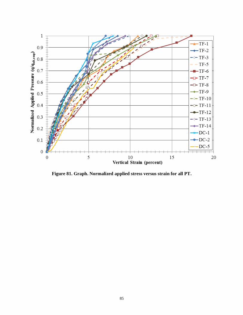
85
Figure 81. Graph. Normalized applied stress versus strain for all PT.

86
Figure 82. Graph. Normalized load-deformation behavior for the DC and TF PTs up to
5-percent vertical strain.

87
7.3 SERVICE LIMIT
FHWA guidance currently recommends a service limit of 4,000 psf applied vertical stress (dead
plus live load, with load factors = 1.0) with a target of 0.5-percent vertical strain for GRS
abutments, measured by using only dead load, unless the engineer decides to permit additional
load and/or deformation.(1)
For a 20-ft-tall wall, the initial compression of the GRS composite
would therefore be limited to 1.2 inches. Note that the majority of compression within a GRS
abutment occurs shortly after placement of dead load, with little post-construction settlement, if
constructed as outlined by FHWA.(5)
The stress-strain curve generated by the PT can immediately be used to estimate deformation. By
knowing the applied dead load, the resulting strain can be found from the PT results.
Alternatively, using a corresponding PT for the particular GRS composite would yield the
amount of dead load (unfactored) that can be placed on the abutment to limit the deformation to
the tolerable amount. For the range of tests conducted in this study (compacted only), the
allowable applied stress is between 1,324 and 6,016 psf (table 8 and figure 84).
Using the normalized load test curves (figure 85), the service stress to meet the 0.5-percent
vertical strain limit is 6 to 23 percent of the ultimate stress, with an average of 13 percent for all
tests. For only the tests with a CMU facing, as would be typical in the field, the range is slightly
narrower, between 8 and 19 percent with an average of 12 percent; for the tests without a facing
element, the average is 15 percent.
When looking strictly at the PTs that meet the current FHWA specifications for a GRS abutment,
the allowable applied stress at low strain levels (i.e., at in-service conditions) ranges between
about 8 percent and 13 percent of the ultimate stress (figure 86), with an average of 10 percent.(1)
By estimating an ultimate stress using the GRS capacity equation (figure 8), ignoring the effects
of cohesion and confining stress as indicated by Adams et al. (2011a) for design of GRS
abutments, and assuming 10 percent of the ultimate capacity, the maximum service stress
(unfactored dead load only) to limit short-term vertical strain to 0.5 percent can be predicted
(table 25).(1)

88
Figure 83. Graph. Cumulative distribution function for proposed service limit pressure.
y = 1.71x - 1.97
R² = 0.95
-2
-1.5
-1
-0.5
0
0.5
1
1.5
2
0 0.5 1 1.5 2 2.5
Sta
nd
ard
Norm
al
Veria
ble
, z
Bias, λ

89
Table 25. Estimation of allowable dead load to limit vertical strain to 0.5 percent using the
GRS capacity equation.
Test
Measured Predicted Bias,
Measured
Predicted
Standard
Normal
Variable, z qult,emp (psf) (psf) , predicted =
10% of qult,an (psf)
DC-1 23,310 3,065 2,974 1.03 -0.34
DC-2 22,709 2,171 2,551 0.85 -0.48
DC-3 N/A 1,324 4,021 0.33 -1.62
DC-4 N/A 2,212 1,655 1.34 0.48
TF-1 20,471 2,068 1,570 1.32 0.20
TF-2 25,260 4,759 2,204 2.16 1.62
TF-3 17,491 3,417 2,204 1.55 1.00
TF-4 N/A 3,705 4,409 0.84 -0.80
TF-5 25,920 6,016 4,409 1.36 0.63
TF-6 43,763 3,704 4,409 0.84 -0.63
TF-7 26,546 2,224 4,409 0.50 -1.00
TF-8 29,134 1,753 4,409 0.40 -1.25
TF-9 22,310 2,955 1,401 2.11 1.25
TF-10 10,330 1,586 1,401 1.13 -0.07
TF-11 23,249 2,839 2,765 1.03 -0.20
TF-12 29,030 4,028 2,765 1.46 0.80
TF-13 12,960 2,398 1,807 1.33 0.34
TF-14 23,562 2,037 1,807 1.13 0.07
Mean Bias 1.15
Standard Deviation 0.58
Coefficient of Variation (percent) 0.51
N/A = Not applicable, did not fail the composite.
The results indicate that by using 10 percent of the predicted design capacity, the mean bias
between the measured results from this series of PTs and the predicted allowable stress at
0.5-percent vertical strain is 1.15 with a COV of 0.51 (table 25). This is on the conservative side
and offers another tool to estimate deformation in lieu of conducting a performance test on a
particular GRS composite.
λ
q@ε=0.5%
q@ε=0.5%

90
Figure 84. Graph. Load-deformation behavior for the Turner Fairbank PTs at low strain
levels.

91
Figure 85. Graph. Normalized load-deformation behavior for the DC and TF PTs up to
0.5-percent vertical strain.

92
Figure 86. Graph. PTs strictly meeting FHWA GRS abutment design specifications.

93
7.4 LRFD CALIBRATION FOR STRENGTH LIMIT
In the United States, bridges that receive federal funding for construction must be designed in
accordance with the AASHTO LRFD Bridge Design Specifications. AASHTO first adopted a
load factor design (LFD) in 1977 for certain portions of the bridge superstructure. In the mid-
1990s, the AASHTO Specifications adopted LRFD in geotechnical engineering design based on
the work of Barker et al. (1991).(35)
Since then, LRFD research has extended to more and more
aspects of geotechnical structures.
LRFD in geotechnical design of bridge and building foundations has the following benefits:
1. Efficiency in design effort can be achieved when using the same factored loads for both
superstructure and sub-structure design.
2. More consistent margins of safety can be realized in both superstructure and sub-structure
design.
3. More economical use of materials can be accomplished when a more rational basis for setting
the margin of safety is provided.
A methodology for calibrating the load bearing capacity (strength limit state) of bridge
foundations on a GRS abutment is described and presented. Calibration for serviceability limit
state is just as, if not more important, since most shallow foundation designs are governed more
by serviceability rather than the ultimate limit state; however, the scope of this report is limited
to only the strength limit state.(10)
7.4.1 Background
Code calibration is the process of determining values of load and resistance factors. While load
factors have already been well established in the AASHTO code, resistance factors for newer
types of geotechnical structures must be obtained by calibration. Resistance factors can be
calibrated using the following approaches:
1. Judgment.
2. Fitting with Allowable Stress Design (ASD).
3. Reliability theory.
Calibration by judgment was the first approach at arriving code parameters, but it suffers from
non-uniform margins of safety. Calibration by fitting with ASD essentially results in the LRFD
code mimicking the ASD code. It does not necessarily result in more uniform margins of safety
or economy. Calibration by fitting was performed for the internal stability design of GRS
abutments.(1)
The approach adopted herein to calibrate the load bearing capacity of GRS
composites is based on reliability theory, which offers a rational process for optimizing the value
of resistance factor. The results are then compared with those from calibrating by fitting with
ASD.
In general, there are three approaches to estimating resistance factors using reliability analysis:
(1) first order second moment (FOSM); (2) advanced first order second moment (AFOSM) and
(3) Monte Carlo simulation (MCS). FOSM is the simplest and results in resistance factors that

94
are marginally lower (more conservative) than the AFOSM method, which requires
programming of an optimization routine. MCS is only accurate if the load and resistance
distributions are correctly modeled. According to Paikowsky (2010), if the statistical parameters
are not well-defined, the resulting resistance factor using MCS will not be correct; moreover, if
the load and resistance distribution is assumed to be lognormal, MCS will theoretically produce
the same results as the FOSM method.(36)
Thus, the simpler FOSM approach is adopted in this
report.
In the reliability-based approach, the load (Q) and resistance (R) are considered random
variables, which can be described by their own probability density functions. One form of
margin of safety can be expressed by the difference R – Q where failure occurs when R – Q < 0.
In the FOSM approach, R and Q are assumed to have a lognormal distribution; hence a limit
state function can be written (figure 87) which is also lognormal. Failure occurs when R/Q is less
than 1 or when g(R,Q) is less than 0. The probability density function of figure 87 is shown in
figure 88.
Figure 87. Equation. Limit state function for FOSM approach.
Figure 88. Graph. Reliability index for lognormal R and Q.
The reliability index ( ) is the number of standard deviations between the mean safety margin
(ḡ) and failure, where g(R,Q) = 0. According to Paikowsky (2010), many shallow foundations
supporting bridge elements have been designed with a target reliability index ( ) between 3.0
and 3.5, which corresponds to a probability of failure of 0.135 percent and 0.023 percent,
respectively.(36)
Note that these target reliability indices are for foundations on natural soil
whereas GRS is an engineered fill.
7.4.2 Reliability Analysis: FOSM
In LRFD, the factored resistance must be greater than or equal to the factored loads (figure 89).
β
βT
g(R,Q) = In(R/Q)

95
Figure 89. Equation. LRFD format.
Where = resistance factor, = load factor for load component i, R = resistance and Qi = load
component i (e.g., dead load or live load). Many load combinations exist in the AASHTO code;
however, resistance factors herein are calibrated using the Strength I load combination only.
With only dead and live loads considered, it can be shown that the resistance factor based on
FOSM can be calculated according to figure 90.
Figure 90. Equation. Resistance factor using FOSM.
Where , ,and are bias factors for resistance, dead load and live load, respectively,
and are the dead (1.25 for AASHTO assuming Strength I load combination and assuming
dead load of structural components and non-structural attachments only; dead load due to the
wearing surface is not considered as it usually represents only a small fraction of the total dead
weight) and live (1.75 for AASHTO assuming Strength I load combination) load factors,
respectively, and VR and VQ are the coefficients of variation (COV) of the resistance and loads,
respectively. The bias factor, , is the ratio of the measured to the nominal or calculated value; if
the variable tends to be over-predicted, then the bias factor will be less than 1. Note that the COV
for a variable that is related to several statistically independent variables is merely the square
root of the sum of the squares of the various coefficients of variation. For example, figure 91
shows that the COV for factored load (VQ) is equal to the sum of the squares of the COV for
dead load (VD) and live load (VL).
Figure 91. Equation. Coefficient of variation for factored load.
It can be seen that in the FOSM method to estimate the resistance factor (figure 90), the random
variables are characterized by their first two moments, namely the mean and the standard
deviation (which is equal to the product of the coefficient of variation and the mean). Therefore,
it is essential to compile the statistics of the load and resistances prior to calibration.
𝚽𝑹 ≥ 𝜸𝒊𝑸𝒊
𝒏
𝒊=𝟏
Φ i
𝚽 =𝝀𝒓 𝜸𝑫
𝑸𝑫
𝑸𝑫 + 𝑸𝑳 / 𝟏 −
𝑸𝑫
𝑸𝑫 + 𝑸𝑳 + 𝜸𝑳
𝜸𝑫 𝑸𝑫
𝑸𝑫 + 𝑸𝑳 / 𝟏 −
𝑸𝑫
𝑸𝑫 + 𝑸𝑳 + 𝜸𝑳
𝟏 + 𝑽𝑹𝟐
𝟏 + 𝑽𝑸𝟐 𝒆
𝜷𝑻 𝒍𝒏 𝟏+𝑽𝑹𝟐 𝟏+𝑽𝑸
𝟐 𝒊
R D L D L
λ
𝐕𝑸 = 𝑽𝑫𝟐 + 𝑽𝑳
𝟐𝟐

96
Load Statistics
In the final report to the National Cooperative Highway Research Program (NCHRP) Project
No. 20-7/186, Kulicki et al. (2007) provided bias factors and COVs for dead and live loads
(table 26).(37)
Thus, from (figure 91) and table 26, the COV for factored load is equal to
15.6 percent.
Table 26. Statistics for dead and live loads.
Dead Load1 Live Load
2
Bias Factor = 1.05 = 1.14
COV VD = 10% VL = 12% 1Assumes cast-in-place concrete elements only.
2Assumes HL-93 loading
for shear and an average daily truck traffic
(ADTT) of 1,000 for two loaded lanes.(10,37)
Resistance Statistics
The variables in the soil-geosynthetic capacity equation (figure 8) and the required reinforcement
strength equation (figure 10) include the maximum aggregate size (dmax), the reinforcement
strength (Tf) and the passive earth pressure coefficient (Kpr); it is reasonable to assume that the
reinforcement spacing (Sv) is not a random variable, therefore the associated fabrication factor is
assumed to be unity. Therefore, the COV of the resistance (VR) can be expressed according to
figure 92.
Figure 92. Equation. Coefficient of variation for resistance.
Where Vdmax, VTf, VKp and VM are the COVs of dmax, Tf, Kp and the capacity model, respectively.
Note that the ultimate reinforcement strength is usually measured in the laboratory under
unconfined conditions; however, it should ideally be measured under confinement to replicate
actual in-service conditions. Benjamin et al. (2008) performed numerous measurements of
reinforcement strength for woven and non-woven geotextiles in the ground and found the COV
for reinforcement strength (VTf) of woven geotextiles was 2.3 and 4.25 percent for the cross-
machine and machine directions, respectively.(38)
Since woven geotextiles were used in the PTs
and are the most commonly used geosynthetic in GRS abutments and IBSs, a VTf value of
4 percent is utilized in this study. For the COV for the passive earth pressure coefficient (VKp),
NCHRP Report 651 recommended a value of 15 percent when measuring friction angles with lab
tests.(36)
The COV for maximum aggregate size (Vdmax) has not yet been investigated, but it is
expected to be small; for one reason, the quarries will set their crushers to a given maximum
grain size with a high degree of certainty. A value of Vdmax = 5 percent is therefore assumed in
this calibration. Additionally, the mean bias factor for the capacity prediction model, using only
the data produced in this study, is 0.88 with a COV of about 35 percent (table 23). The resulting
COV for resistance (VR) is estimated at 39 percent.
D L
𝐕𝑹 = 𝑽𝒅𝒎𝒂𝒙𝟐 + 𝑽𝑻𝒇
𝟐 + 𝑽𝑲𝒑
𝟐 + 𝑽𝑴𝟐𝟐

97
7.4.3 Resistance Factor
The database of results from this study consists of sixteen cases taken to failure of the GRS
composite, four with open-graded backfill (DC-1, DC-2, DC-5, and TF-1) and twelve with well-
graded backfill material (TF-2, TF-3, and TF-5 to TF-14). Because the number of cases with
open-graded backfill is limited, the present strategy is to arrive at one value for the resistance
factor that is applicable to all conditions. With additional testing in the future, separate resistance
factors can be calibrated for each soil type, if necessary.
The resistance factor for GRS capacity, calculated according to figure 90, is presented as a
function of the ratio of dead load to total load, QD/(QD + QL), and the target reliability index ( )
in figure 93. Note that a QD/(QD + QL) of 0.5 corresponds approximately to a bridge span of
about 60 ft, whereas a QD/(QD + QL) of 0.2 corresponds to a bridge span of approximately
250 ft.(39)
The bridge span for a GRS-IBS is currently limited to 140 ft (Adams et al. 2011);
therefore the resistance factors of interest correspond to QD/(QD + QL) greater than about 0.32.
Over this range, the resistance factor varies from 0.26 to 0.28 for = 3.5, from 0.32 to 0.34 for
= 3.0, and from 0.40 to 0.41 for = 2.5 using FOSM.
Figure 93. Graph. Resistance factor for footings on GRS composites for different dead to
dead plus live load ratios and target reliability indices based on PT series.
Similarly, a reliability analysis was performed using the results of all prior GRS composite
testing with a mean bias of 0.95 and a COV for the model of 32 percent (table 24). This slightly
increases the resistance factor for the same target reliability indices (figure 94); for the range of
QD/(QD + QL) greater than 0.32, the resistance factor varies from 0.31 to 0.33 for = 3.5, from
0.38 to 0.39 for = 3.0, and from 0.46-0.48 for = 2.5 using FOSM.
βT
βT
βT βT
βT
βT βT

98
The resistance factors found through the reliability analysis using the standard reliability indices
of 3.0 and 3.5 for bridge foundations are lower than the resistance factor found through
calibration by fitting to ASD. For a factor of safety (FS) of 3.5, a resistance factor of 0.45 was
estimated for the soil-geosynthetic capacity equation.(1)
Through back-calculation, this equates to
a reliability index ( ) of about 2.5.
In NCHRP Report 507, Paikowsky et al. (2004) suggested that for redundant foundation systems
(such as pile groups), a reliability index of 2.3 was appropriate.(40)
With the frequency of the
reinforcement spacing, GRS composites can be considered a redundant foundation system as
well, with no catastrophic collapse observed at failure for any of the PTs. In addition, Bathurst et
al. (2008) suggest that a reliability index of 2.3 is appropriate for the internal stability of
reinforced soil walls.(41)
This leads to the conclusion that the currently used resistance factor of
0.45, having a reliability index of 2.5, is reasonable for design.
Figure 94. Graph. Resistance factor for footings on GRS composites for different dead to
dead plus live load ratios and target reliability indices based on all testing to date.
β
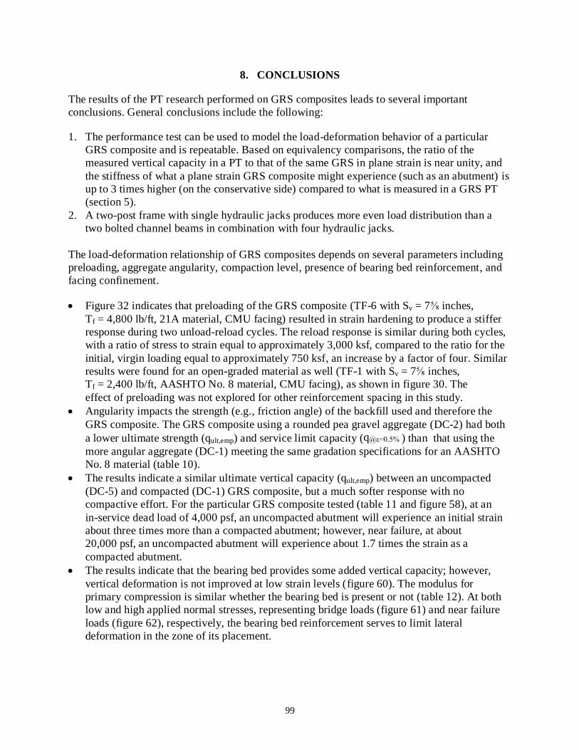
99
8. CONCLUSIONS
The results of the PT research performed on GRS composites leads to several important
conclusions. General conclusions include the following:
1. The performance test can be used to model the load-deformation behavior of a particular
GRS composite and is repeatable. Based on equivalency comparisons, the ratio of the
measured vertical capacity in a PT to that of the same GRS in plane strain is near unity, and
the stiffness of what a plane strain GRS composite might experience (such as an abutment) is
up to 3 times higher (on the conservative side) compared to what is measured in a GRS PT
(section 5).
2. A two-post frame with single hydraulic jacks produces more even load distribution than a
two bolted channel beams in combination with four hydraulic jacks.
The load-deformation relationship of GRS composites depends on several parameters including
preloading, aggregate angularity, compaction level, presence of bearing bed reinforcement, and
facing confinement.
Figure 32 indicates that preloading of the GRS composite (TF-6 with Sv = 7⅝ inches,
Tf = 4,800 lb/ft, 21A material, CMU facing) resulted in strain hardening to produce a stiffer
response during two unload-reload cycles. The reload response is similar during both cycles,
with a ratio of stress to strain equal to approximately 3,000 ksf, compared to the ratio for the
initial, virgin loading equal to approximately 750 ksf, an increase by a factor of four. Similar
results were found for an open-graded material as well (TF-1 with Sv = 7⅝ inches,
Tf = 2,400 lb/ft, AASHTO No. 8 material, CMU facing), as shown in figure 30. The
effect of preloading was not explored for other reinforcement spacing in this study.
Angularity impacts the strength (e.g., friction angle) of the backfill used and therefore the
GRS composite. The GRS composite using a rounded pea gravel aggregate (DC-2) had both
a lower ultimate strength (qult,emp) and service limit capacity ( ) than that using the
more angular aggregate (DC-1) meeting the same gradation specifications for an AASHTO
No. 8 material (table 10).
The results indicate a similar ultimate vertical capacity (qult,emp) between an uncompacted
(DC-5) and compacted (DC-1) GRS composite, but a much softer response with no
compactive effort. For the particular GRS composite tested (table 11 and figure 58), at an
in-service dead load of 4,000 psf, an uncompacted abutment will experience an initial strain
about three times more than a compacted abutment; however, near failure, at about
20,000 psf, an uncompacted abutment will experience about 1.7 times the strain as a
compacted abutment.
The results indicate that the bearing bed provides some added vertical capacity; however,
vertical deformation is not improved at low strain levels (figure 60). The modulus for
primary compression is similar whether the bearing bed is present or not (table 12). At both
low and high applied normal stresses, representing bridge loads (figure 61) and near failure
loads (figure 62), respectively, the bearing bed reinforcement serves to limit lateral
deformation in the zone of its placement.
q@ε=0.5%

100
The frictionally connected CMU facing has an impact on the performance of GRS; it
provides confinement, leading to a stiffer response and an increased capacity compared to a
GRS composite with no facing element. From table 20, the facing more than doubles the
initial stress-strain ratio as compared to the PTs without any facing. In terms of capacity, the
facing plays the biggest and smallest role for the largest spaced (Sv = 15¼ inches) and the
closest spaced (Sv = 313
/16 inches) system tested, respectively. For the 5 pairs of tests
conducted at TF, including the CMU facing produced an improved ultimate capacity between
1.2 and 2.2 times greater than the GRS composite without any facing (table 21). A similar
trend to the strain at the current 4,000-psf service limit is also found. The design assumption
to not include the effect of confinement from the face in determining the capacity and
required reinforcement strength is therefore conservative.(1)
In addition, at the current service stress limit (applied stress, q, of 4,000 psf), the ratio of
service vertical strain with no facing to service vertical strain with a CMU facing ranges from
1.2 to 2.2 (table 21). The largest impact was for the 15⅝-inch spaced GRS composite (TF-9
and TF-10). At ultimate failure, the ratio is considerably closer, ranging from 0.8 to 1.2.
For the same Tf/Sv ratio of 3,800 lb/ft2, there is a linear relationship between the
reinforcement spacing (Sv) and the ratio of capacity with CMU facing (qult,emp CMU) to the
capacity without facing (qult,emp no CMU) (figure 75). Similarly, there is a linear relationship
with reinforcement strength (figure 76).
Both open-graded and well-graded aggregates can be used as the reinforced backfill in GRS
composites; each has their advantages and disadvantages. The PT results further distinguished
the effect aggregate selection can have on the behavior of GRS.
The well-graded material is considerably stiffer than the open-graded material. At an applied
pressure of 4,000 psf, the vertical strain is about 1.1 percent for TF-1 (open-graded) and
0.4 percent for TF-2 (well-graded). The modulus of the composite tested in TF-1 is 320 ksf
(table 13) compared to 710 ksf for the composite tested in TF-2; TF-1 (open-graded) is
55 percent less stiff than TF-2 (well-graded). In terms of bearing capacity, TF-1 was
20 percent less strong than TF-2. The results indicate that the gradation, and perhaps
cohesion (at the same friction angle), impacts the modulus more so than the strength, giving
indication that well-graded fills have an advantage with respect to serviceability.
As discussed in section 6.1, isolating the effect of cohesion and other soil parameters on the
performance of GRS is difficult using PTs, although based on the soil-geosynthetic capacity
equation (figure 8), it will serve to improve capacity, although its contribution should not be
considered in design.
The response indicates that the higher reinforcement strength (4,800 lb/ft) produces a stiffer
and stronger response than the lower reinforcement strength (2,400 lb/ft) for open-graded
backfill (table 15); the same is true for the composites with no facing element. By doubling
the reinforcement strength, the results indicate an increase of measured capacity by a factor
of 1.14 for capacity and 1.34 for the initial stress-strain ratio.
For the well-graded aggregate, increasing the reinforcement strength increases the capacity
by a factor of 1.5 and 1.7 for no facing and CMU facing (table 16), respectively, but does not
significantly impact the stiffness.

101
The relationship between reinforcement strength and spacing was investigated through a series of
PTs with the same Tf/Sv ratio.
The response for experiments conducted with a Tf/Sv ratio of 3,800 lb/ft2 showed that as
reinforcement spacing increased, the vertical capacity decreased for the same T f/Sv ratio,
whether a CMU facing was absent (figure 66) or present (figure 67). This suggests that the
relationship between reinforcement strength and spacing is not proportional to capacity as
outlined in current MSE design (AASHTO 2012); a GRS abutment with a given T f and Sv
will not have the same strength as a GRS abutment with twice the strength (2T f) and
reinforcement spacing (2Sv).
At the same Tf/Sv ratio of 3,800 lb/ft2, increasing the reinforcement spacing by a factor of
two from 7⅝ to 15¼ inches and the reinforcement strength by a factor of two from
2,400 to 4,800 lb/ft, resulted in a reduction of the capacity by a factor of 0.9 and 0.6 for CMU
facing and no facing, respectively. The relationship is therefore not directly proportional, as
indicated for MSE design (AASHTO 2012).
The primary purpose of PTs is to provide a designer with the unique stress-strain properties of a
particular GRS composite for use in design. There is an empirical method and an analytical
method currently available for GRS by FHWA.(1)
Note that only 3 GRS composites tested in this study meet both the design limits and the
material specifications (e.g., Tf ≥ 4,800 lb/ft, dmax ≥ ½ inches) for GRS abutments; however,
based on the results of this study, perhaps the criteria can be amended to reduce the
reinforcement strength limitation, provided the reinforcement strength meets internal stability
design requirements.(1)
Based on the results of the PTs presented in this report, the average bias for the capacity
equation is 0.88 with a COV of about 35 percent (table 23). Including the results from other
sources in the literature, the average bias is 0.95 with a COV of about 32 percent. These
numbers indicate relatively good agreement between figure 8 and the measured ultimate
capacity (table 24).
The 5-percent vertical strain limit can significantly reduce the allowable stress placed on a
GRS composite; figure 82 shows that at 5-percent strain, the applied pressure is between 50
and 85 percent of the measured ultimate capacity (table 8).
The results indicate that by using 10 percent of the predicted design capacity (figure 8), the
0.5-percent vertical strain as required by FHWA for the service limit of GRS abutments can
largely be satisfied. The mean bias of the ratio between the measured results at 0.5-percent
vertical strain from this series of PTs and the predicted allowable stress at 10 percent of the
design capacity is 1.15 with a COV of 0.51 (table 25). This is on the conservative side yet
offers another tool to estimate deformation in lieu of conducting a performance test on a
particular GRS composite.
Finally, a reliability analysis for the soil-geosynthetic capacity equation (figure 8) was performed
on the 16 PTs taken to failure in this study, along with previous results from additional GRS
testing found from the literature.
102
A target reliability index of 2.5 is reasonable for the strength limit models for GRS
composites designed according to Adams et al. (2011). A lower target reliability index is
warranted for closely-spaced GRS composites because of the redundancy in the
reinforcement and because no catastrophic collapse was observed in any of the performance
tests at failure. In addition, Bathurst et al. (2008) suggest that a reliability index of 2.3 is
appropriate for the internal stability of reinforced soil walls.(1,41)
Performing a reliability analysis using the FOSM approach produces a resistance factor
around 0.45, similar to that found through calibration by fitting to ASD methods.
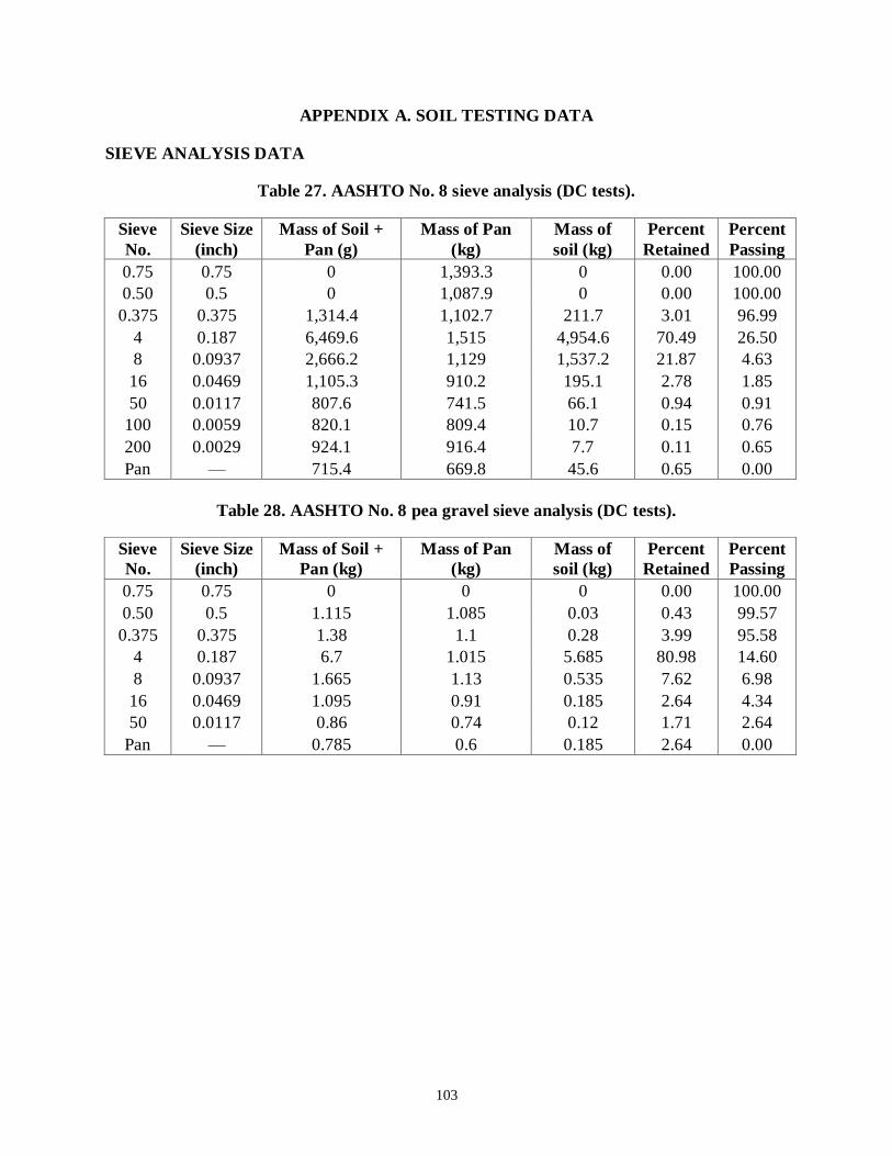
103
APPENDIX A. SOIL TESTING DATA
SIEVE ANALYSIS DATA
Table 27. AASHTO No. 8 sieve analysis (DC tests).
Sieve
No.
Sieve Size
(inch)
Mass of Soil +
Pan (g)
Mass of Pan
(kg)
Mass of
soil (kg)
Percent
Retained
Percent
Passing
0.75 0.75 0 1,393.3 0 0.00 100.00
0.50 0.5 0 1,087.9 0 0.00 100.00
0.375 0.375 1,314.4 1,102.7 211.7 3.01 96.99
4 0.187 6,469.6 1,515 4,954.6 70.49 26.50
8 0.0937 2,666.2 1,129 1,537.2 21.87 4.63
16 0.0469 1,105.3 910.2 195.1 2.78 1.85
50 0.0117 807.6 741.5 66.1 0.94 0.91
100 0.0059 820.1 809.4 10.7 0.15 0.76
200 0.0029 924.1 916.4 7.7 0.11 0.65
Pan — 715.4 669.8 45.6 0.65 0.00
Table 28. AASHTO No. 8 pea gravel sieve analysis (DC tests).
Sieve
No.
Sieve Size
(inch)
Mass of Soil +
Pan (kg)
Mass of Pan
(kg)
Mass of
soil (kg)
Percent
Retained
Percent
Passing
0.75 0.75 0 0 0 0.00 100.00
0.50 0.5 1.115 1.085 0.03 0.43 99.57
0.375 0.375 1.38 1.1 0.28 3.99 95.58
4 0.187 6.7 1.015 5.685 80.98 14.60
8 0.0937 1.665 1.13 0.535 7.62 6.98
16 0.0469 1.095 0.91 0.185 2.64 4.34
50 0.0117 0.86 0.74 0.12 1.71 2.64
Pan — 0.785 0.6 0.185 2.64 0.00

104
Table 29. AASHTO No. 57 Sieve analysis (DC tests).
Sieve
No.
Sieve Size
(inch)
Mass of Soil +
Pan (g)
Mass of Pan
(kg)
Mass of
soil (kg)
Percent
Retained
Percent
Passing
1.5 1.5 1,476.1 1,476.1 0 0.00 100.00
1 1 1,127.1 1,127.1 0 0.00 100.00
0.75 0.75 2,311 1,393.4 917.6 12.09 87.91
0.50 0.5 5,052.1 1,087.8 3,964.3 52.22 35.69
0.375 0.375 2,739.5 1,102.7 1,636.8 21.56 14.13
4 0.187 2,308.8 1,514.8 794 10.46 3.67
8 0.0937 1,224.5 1,128.9 95.6 1.26 2.41
16 0.0469 981.1 909.8 71.3 0.94 1.47
200 0.0029 974.5 916.7 57.8 0.76 0.71
Pan — 723.3 669.7 53.6 0.71 0.00
Table 30. AASHTO No. 9 Sieve analysis (DC tests).
Sieve
No.
Sieve Size
(inch)
Mass of Soil +
Pan (g)
Mass of Pan
(kg)
Mass of
soil (kg)
Percent
Retained
Percent
Passing
0.75 0.75 0 1,393.21 0 0.00 100.00
0.50 0.5 0 1,087.95 0 0.00 100.00
0.375 0.375 0 1,102.79 0 0.00 100.00
4 0.187 1,785.33 1,514.98 270.35 5.78 94.22
8 0.0937 4,236.2 1,129.04 3,107.16 66.47 27.75
16 0.0469 1,791.1 909.95 881.15 18.85 8.90
50 0.0117 986.6 741.69 244.91 5.24 3.66
100 0.0059 830 809.4 20.6 0.44 3.22
200 0.0029 934.9 916.46 18.44 0.39 2.82
Pan — 732.6 600.56 132.04 2.82 0.00

105
Table 31. AASHTO No. 8 Sieve analysis (TFHRC tests).
Sieve
No.
Sieve Size
(inch)
Mass of Soil +
Pan (g)
Mass of Pan
(kg)
Mass of
soil (kg)
Percent
Retained
Percent
Passing
1 1 1,127.1 1,127.1 0 0.00 100.00
0.50 0.5 1,116.5 1,087.7 28.8 0.31 99.69
0.375 0.375 3,832 1,102.6 2,729.4 29.83 69.86
4 0.187 6,694.3 1,013.8 5,680.5 62.08 7.78
8 0.0937 1,688.5 1,128.7 559.8 6.12 1.66
10 0.079 1,398.7 1,374 24.7 0.27 1.39
16 0.0469 935 909.7 25.3 0.28 1.11
40 0.0165 810 793.1 16.9 0.18 0.93
50 0.0117 746.2 741.8 4.4 0.05 0.88
Pan — 750.4 669.8 80.6 0.88 0.00
Table 32. AASHTO A-1-a (VDOT 21A) sieve analysis (TFHRC tests).
Sieve
No.
Sieve Size
(inch)
Mass of Soil +
Pan (g)
Mass of Pan
(kg)
Mass of
soil (kg)
Percent
Retained
Percent
Passing
1 1 1,127.1 1,127.1 0 0.00 100.00
0.50 0.5 1,919.2 1,087.6 831.6 17.59 82.41
0.375 0.375 1,624.9 1,102.7 522.2 11.05 71.36
4 0.187 2,093.7 1,013.8 1,079.9 22.84 48.52
8 0.0937 1,757.5 1,129.6 627.9 13.28 35.24
10 0.079 1,489.5 1,374.7 114.8 2.43 32.81
16 0.0469 1,260.5 910.1 350.4 7.41 25.40
40 0.0117 1,206.5 793.1 413.4 8.74 16.66
200 0.0029 1,397.8 916.5 481.3 10.18 6.47
Pan — 975.7 669.6 306.1 6.47 0.00

106
LSDS TESTING DATA
Table 33. Summary of AASHTO No. 8 LSDS results (DC tests).
Soil
Type
Normal
Stress (psi)
Max Shear
(psi)
Peak Friction
Angle (°)
Peak Dilation
Angle (°)
Gap
(inch)
8 5.051 9.5114 62.03 12.96 0.343
8 10.03 19.0619 62.25 11.65 0.343
8 20.03 30.533 56.73 6.35 0.343
8 30.02 45.6537 56.67 5.63 0.343
Figure 95. Graph. AASHTO No. 8 LSDS test results (DC tests).
0
5
10
15
20
25
30
35
40
45
50
0 0.5 1 1.5 2
Sh
ear
Str
ess
(p
si)
Horizontal Displacement (inch)
5 psi
10 psi
20 psi
30 psi

107
Figure 96. AASHTO No. 8 LSDS deformation test results (DC tests).
Table 34. Summary of AASHTO No. 8 pea gravel LSDS results (DC tests).
Soil
Type
Normal
Stress (psi)
Max Shear
(psi)
Peak Friction
Angle (°)
Peak Dilation
Angle (°)
Gap
(inch)
8P 5.022 7.5449 56.35 13.19 0.35
8P 10.05 15.00489 56.19 11.79 0.35
8P 20.01 21.238 46.71 5.96 0.35
8P 30.01 35.1467 49.51 6.04 0.35
-0.25
-0.2
-0.15
-0.1
-0.05
0
0.05
0 0.5 1 1.5 2
Verti
ca
l D
isp
lacem
en
t (i
nch
)
Horizontal Displacement (inch)
5 psi
10 psi
20 psi
30 psi

108
Figure 97. Graph. AASHTO No. 8 pea gravel LSDS test results (DC tests).
Figure 98. Graph. AASHTO No. 8 pea gravel LSDS deformation test results (DC tests).
-0.25
-0.2
-0.15
-0.1
-0.05
0
0.05
0 1 2 3
Verti
ca
l D
isp
lacem
en
t (i
nch
)
Horizontal Displacement (inch)
5 psi
10 psi
20 psi
30 psi
0
5
10
15
20
25
30
35
40
0 1 2 3
Sh
ear
Str
ess
(p
si)
Horizontal Displacement (inch)
5 psi
10 psi
20 psi
30 psi

109
Table 35. Summary of AASHTO No. 57 LSDS results (DC tests).
Soil
Type
Normal
Stress (psi)
Max Shear
(psi)
Peak Friction
Angle (°)
Peak Dilation
Angle (°)
Gap
(inch)
57 5.013 17.547 74.06 15.36 0.74
57 10.01 21.187 64.71 13.15 0.74
57 20.04 40.212 63.51 9.93 0.74
57 30.01 47.189 57.55 6.28 0.74
Figure 99. Graph. AASHTO No. 57 LSDS test results (DC tests).
0
5
10
15
20
25
30
35
40
45
50
0 1 2 3
Sh
ea
r S
tress
(p
si)
Horizontal Displacement (inch)
5 psi
10 psi
20 psi
30 psi

110
Figure 100. Graph. AASHTO No. 57 LSDS deformation test results (DC tests).
Table 36. Summary of AASHTO No. 9 LSDS results (DC tests).
Soil
Type
Normal
Stress (psi)
Max Shear
(psi)
Peak Friction
Angle (°)
Peak Dilation
Angle (°)
Gap
(inch)
9 5.053 9.7334 62.56 13.64 0.175
9 10.04 17.698 60.43 10.38 0.175
9 20.01 31.97 57.96 5.82 0.175
9 30.02 42.8381 54.98 4.73 0.175
-0.35
-0.3
-0.25
-0.2
-0.15
-0.1
-0.05
0
0.05
0 1 2 3
Verti
ca
l D
isp
lacem
en
t (i
nch
)
Horizontal Displacement (inch)
5 psi
10 psi
20 psi
30 psi

111
Figure 101. Graph. AASHTO No. 9 LSDS test results (DC tests).
Figure 102. Graph. AASHTO No. 9 LSDS deformation test results (DC tests).
0
5
10
15
20
25
30
35
40
45
0 1 2 3
Sh
ear
Str
ess
(p
si)
Horizontal Displacement (inch)
5 psi
10 psi
20 psi
30 psi
-0.2
-0.15
-0.1
-0.05
0
0.05
0 1 2 3
Verti
ca
l D
isp
lacem
en
t (i
nch
)
Horizontal Displacement (inch)
5 psi
10 psi
20 psi
30 psi

112
Table 37. Summary of AASHTO No. 8 LSDS results (TFHRC tests).
Soil
Type
Normal
Stress (psi)
Max Shear
(psi)
Peak Friction
Angle (°)
Peak Dilation
Angle (°)
Gap
(inch)
8 5.04 15.220948 71.68 15.66 0.443
8 10.06 26.73174 69.38 11.01 0.443
8 20.03 39.8865 63.34 8.07 0.443
8 30.02 52.54942 60.26 5.10 0.443
Figure 103. Graph. AASHTO No. 8 LSDS test results (TFHRC tests).
0
10
20
30
40
50
60
0 1 2 3
Sh
ea
r S
tress
(p
si)
Horizontal Displacement (inch)
5 psi
10 psi
20 psi
30 psi

113
Figure 104. Graph. AASHTO No. 8 LSDS deformation test results (DC tests).
Table 38. Summary of AASHTO A-1-a (VDOT 21A) LSDS results (TFHRC tests).
Soil
Type
Test
Condition
Normal
Stress
(psi)
Max
Shear
(psi)
Peak
Friction
Angle (°)
Peak
Dilation
Angle (°)
Gap (inch)
21A Dry 5.046 17.305 73.74 26.08 0.58
21A Dry 10.05 23.6762 67.00 20.48 0.58
21A Dry 20.02 40.35021 63.61 12.58 0.58
21A Dry 30.03 50.135 59.08 11.05 0.58
21A Saturated 4.99 5.46532 47.60 0.00 0.58
21A Saturated 9.991 14.2569 54.98 0.05 0.58
21A Saturated 19.98 25.034 51.41 0.00 0.58
21A Saturated 29.99 36.2423 50.39 0.00 0.58
-0.4
-0.35
-0.3
-0.25
-0.2
-0.15
-0.1
-0.05
0
0.05
0 1 2 3
Verti
ca
l D
isp
lacem
en
t (i
nch
)
Horizontal Displacement (inch)
5 psi
10 psi
20 psi
30 psi

114
Figure 105. Graph. AASHTO A-1-a (VDOT 21A) LSDS test results (TFHRC tests).
Figure 106. Graph. AASHTO A-1-a (VDOT 21A) LSDS deformation test results (DC tests).
0
10
20
30
40
50
60
0 0.5 1 1.5 2 2.5 3
Sh
ear
Str
ess
(p
si)
Horizontal Displacement (inch)
5 psi
10 psi
20 psi
30 psi
-0.5
-0.4
-0.3
-0.2
-0.1
0
0.1
0 1 2 3
Verti
ca
l D
isp
lacem
en
t (i
nch
)
Horizontal Displacement (inch)
5 psi
10 psi
20 psi
30 psi

115
APPENDIX B. NUCLEAR DENSITY TESTING FOR TFHRC PTS
Table 39. TF-2 Nuclear density test results.
Lift
Depth
(inch) (pcf)
Percent of
Proctor (percent)
1 backscatter 107.8 95.6 1.2
backscatter 109.2 96.8 1.4
2 4 107 94.8 1.4
6 112.8 100.0 1.2
3 4 101 89.5 1.1
6 104.6 92.7 0.8
4 4 109.9 97.4 1
6 110 97.5 1
5 4 111.6 98.9 0.7
6 114.7 101.7 0.8
6 4 109.1 96.7 1.7
6 111 98.4 1.3
7 4 110.9 98.3 1.9
6 110.7 98.1 0.9
8 4 117.2 103.9 1.2
6 113.4 100.5 1.4
9 4 111.4 98.7 1.1
6 115 101.9 0.8
10 4 111.7 99.0 1.9
6 110.3 97.8 0.9
γd ω

116
Table 40. TF-2 Nuclear density test results.
Lift
Depth
(inch)
(pcf)
Percent of
Proctor
(percent)
1 4 148.5 99.7 5.5
6 149.8 100.6 7.2
2 4 147 98.7 6.7
6 145.5 97.7 6
3 4 145.6 97.8 6.9
6 147.6 99.1 6.3
4 4 141.9 95.3 6.6
6 141.5 95.0 6.3
5 4 147.2 98.9 5.9
6 148.6 99.8 6.2
6 4 145.5 97.7 6.2
6 146.2 98.2 6.8
7 4 146.4 98.3 6.4
6 145.8 97.9 5.8
8 4 147.3 98.9 6
6 146.2 98.2 6.1
9 4
6
10 4
6
Blank cell = no data available.
γd ω

117
Table 41. TF-3 Nuclear density test results.
Lift
Depth
(inch)
(pcf)
Percent of
Proctor
(percent)
1 4 147.9 99.3 6.7
6 148.1 99.5 7
2 4 146.1 98.1 6.7
6 150.8 101.3 6.6
3 4 147.4 99.0 6.2
6 149 100.1 5.9
4 4 146.2 98.2 6.8
6 149.5 100.4 6.1
5 4 149.7 100.5 5.5
6 149.1 100.1 6.5
6 6 147.3 98.9 7.8
7 6 147.2 98.9 7.9
8 6 149.3 100.3 6.4
9 6 151.3 101.6 6.1
10 6 151.1 101.5 6.6
Table 42. TF-4 Nuclear density test results.
Lift
Depth
(inch)
(pcf)
Percent of
Proctor ω
(percent)
1 4 149.2 100.2 6.3
2 6 147.6 99.1 6.3
3 6 147.7 99.2 6.2
4 6 147.9 99.3 7.3
5 6 149 100.1 7
6 6 149.7 100.5 7.1
7 6 149.4 100.3 6.8
8 6 151.1 101.5 6.2
9 6 152.6 102.5 5.6
10 6 151.1 101.5 6.8
γd ω
γd
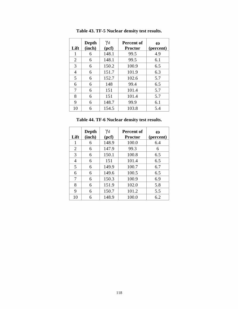
118
Table 43. TF-5 Nuclear density test results.
Lift
Depth
(inch)
(pcf)
Percent of
Proctor
(percent)
1 6 148.1 99.5 4.9
2 6 148.1 99.5 6.1
3 6 150.2 100.9 6.5
4 6 151.7 101.9 6.3
5 6 152.7 102.6 5.7
6 6 148 99.4 6.5
7 6 151 101.4 5.7
8 6 151 101.4 5.7
9 6 148.7 99.9 6.1
10 6 154.5 103.8 5.4
Table 44. TF-6 Nuclear density test results.
Lift
Depth
(inch)
(pcf)
Percent of
Proctor
(percent)
1 6 148.9 100.0 6.4
2 6 147.9 99.3 6
3 6 150.1 100.8 6.5
4 6 151 101.4 6.5
5 6 149.9 100.7 6.7
6 6 149.6 100.5 6.5
7 6 150.3 100.9 6.9
8 6 151.9 102.0 5.8
9 6 150.7 101.2 5.5
10 6 148.9 100.0 6.2
γd ω
γd ω

119
Table 45. TF-7 Nuclear density test results.
Lift
Depth
(inch)
(pcf)
Percent of
Proctor
(percent)
1 6 150.1 100.8 6.3
2 6 151.2 101.5 5.9
3 6 150.1 100.8 6.2
4 6 149.1 100.1 6.1
5 6 152.3 102.3 6.1
6 6 150.2 100.9 5.8
7 6 151 101.4 5.9
8 6 148.9 100.0 6.3
9 6 149.5 100.4 5.9
10 6 152.5 102.4 5.9
Table 46. TF-8 Nuclear density test results.
Lift
Depth
(inch)
(pcf)
Percent of
Proctor
(percent)
1 6 149.1 100.1 7.1
2 6 148.7 99.9 6.9
3 6 151 101.4 6.4
4 6 150.6 101.1 6.3
5 6 151.5 101.7 6.5
6 6 150.5 101.1 6.5
7 6 151.2 101.5 6.3
8 6 151.1 101.5 6.4
9 2 147.6 99.1 6.2
10 2 146.9 98.7 6.5
10 2 150.8 101.3 5.9
γd ω
γd ω
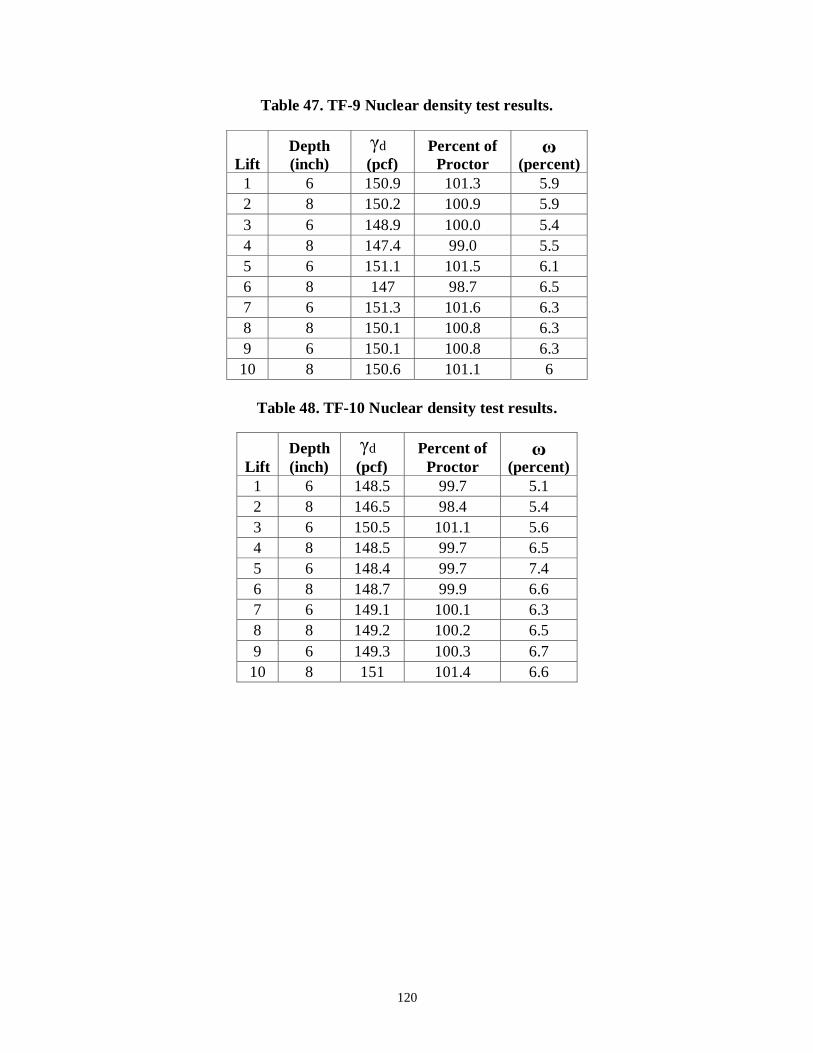
120
Table 47. TF-9 Nuclear density test results.
Lift
Depth
(inch)
(pcf)
Percent of
Proctor
(percent)
1 6 150.9 101.3 5.9
2 8 150.2 100.9 5.9
3 6 148.9 100.0 5.4
4 8 147.4 99.0 5.5
5 6 151.1 101.5 6.1
6 8 147 98.7 6.5
7 6 151.3 101.6 6.3
8 8 150.1 100.8 6.3
9 6 150.1 100.8 6.3
10 8 150.6 101.1 6
Table 48. TF-10 Nuclear density test results.
Lift
Depth
(inch)
(pcf)
Percent of
Proctor
(percent)
1 6 148.5 99.7 5.1
2 8 146.5 98.4 5.4
3 6 150.5 101.1 5.6
4 8 148.5 99.7 6.5
5 6 148.4 99.7 7.4
6 8 148.7 99.9 6.6
7 6 149.1 100.1 6.3
8 8 149.2 100.2 6.5
9 6 149.3 100.3 6.7
10 8 151 101.4 6.6
γd ω
γd ω

121
Table 49. TF-11 Nuclear density test results.
Lift
Depth
(inch)
(pcf)
Percent of
Proctor
(percent)
1 2 148 99.4 6.8
2 150.2 100.9 6.5
2 2 153.2 102.9 5.5
2 149.8 100.6 6.2
3 2 149.8 100.6 6.1
2 150.4 101.0 5.8
4 2 151.8 101.9 5.8
2 151.8 101.9 5.7
5 2 150.6 101.1 6.2
2 148.2 99.5 6.1
6 2 149.9 100.7 5.8
2 149.3 100.3 5.5
7 2 147.4 99.0 5.6
2 150.6 101.1 5.7
8 2 149.9 100.7 5.5
2 150 100.7 5.8
9 2 150.2 100.9 5.4
2 152.3 102.3 5.4
10 2 149.9 100.7 5.8
2 149.8 100.6 5.9
γd ω

122
Table 50. TF-12 Nuclear density test results.
Lift
Depth
(inch)
(pcf)
Percent of
Proctor
(percent)
1 2 149 100.1 6
2 148.7 99.9 5.8
2 2 148.1 99.5 5.7
2 149 100.1 6.3
3 2 150.3 100.9 6.5
2 148.2 99.5 6.6
4 2 149.3 100.3 6.4
2 148.5 99.7 6.0
5 2 147.6 99.1 5.8
2 150.4 101.0 5.9
6 2 148 99.4 6
2 148.8 99.9 5.5
7 2 148.5 99.7 6
2 152.2 102.2 5.6
8 2 147.9 99.3 6.1
2 148 99.4 6.4
9 2 151.1 101.5 6.2
2 149 100.1 6.1
10 2 149.9 100.7 5.0
2 151.1 101.5 5.0
γd ω

123
Table 51. TF-13 Nuclear density test results
Lift
Depth
(inch)
(pcf)
Percent of
Proctor
(percent)
1 4 148 99.4 6.8
4 146.6 98.5 6.3
4 147.4 99.0 5.7
2 4 147.6 99.1 5.8
4 147.8 99.3 5.7
4 150.9 101.3 5.7
3 6 151.9 102.0 6.8
4 150.5 101.1 6.6
4 6 149.9 100.7 6.3
4 147 98.8 5.9
5 8 146.8 98.6 6
4 150.6 101.1 6.4
6 6 152.4 102.4 6
4 148.2 99.50 5.8
7 6 149.4 100.3 5.9
4 153.2 102.9 5.7
Table 52. TF-14 Nuclear density test results.
Lift
Depth
(inch)
(pcf)
Percent of
Proctor
(percent)
1 6 147.8 99.3 4.4
4 150.5 101.1 6.6
2 6 150.6 101.1 6.8
4 148 99.4 5.6
3 6 148.3 99.6 5.8
4 149.7 100.5 5.5
4 6 150.6 101.1 7
4 147.9 99.3 7.4
5 6 147.4 99.0 7.4
4 148.5 99.7 7
6 6 150 100.7 6.2
4 148 99.4 7.1
7 6 150.2 100.9 6.7
4 147.8 99.3 6.6
γd ω
γd ω


125
APPENDIX C. DEFORMATION INSTRUMENTATION LAYOUTS FOR PTS
Figure 107. Illustration. Instrumentation layout for DC tests and TF-1.
Figure 108. Illustration. Instrumentation layout for TF-2, TF-9.

126
Figure 109. Illustration. Instrumentation layout for TF-3, TF-4.
Figure 110. Illustration. Instrumentation layout for TF-5, TF-7.

127
Figure 111. Instrumentation layout for TF-6, TF-12.
Figure 112. Illustration. Instrumentation layout for TF-8.

128
Figure 113. Illustration. Instrumentation layout for TF-10.
Figure 114. Illustration. Instrumentation layout for TF-13

129
Figure 115. Illustration. Instrumentation layout for TF-14.


131
APPENDIX D. RAW DATA FOR PTS
Table 53. DC-1 PT Data.
Average
Load
(lb/jack)
Applied
Pressure
(psf)
Vertical
Settlement
(inch)
Vertical
strain
(percent)
0.00 0.00 0.00 0.00
6,000.29 2,666.80 0.33 0.43
7,691.24 3,418.33 0.43 0.56
10,891.56 4,840.69 0.58 0.76
13,882.17 6,169.85 0.82 1.08
16,743.42 7,441.52 1.02 1.34
18,617.17 8,274.30 1.19 1.56
20,737.31 9,216.58 1.35 1.78
23,679.35 10,524.15 1.56 2.05
26,749.52 11,888.68 1.85 2.43
29,760.19 13,226.75 2.12 2.79
32,796.45 14,576.20 2.60 3.43
36,725.03 16,322.23 2.99 3.93
38,843.79 17,263.90 3.24 4.26
41,800.05 18,577.80 3.57 4.70
45,218.53 20,097.12 3.82 5.02
49,169.75 21,853.22 4.20 5.52
52,488.78 23,328.34 6.04 7.95
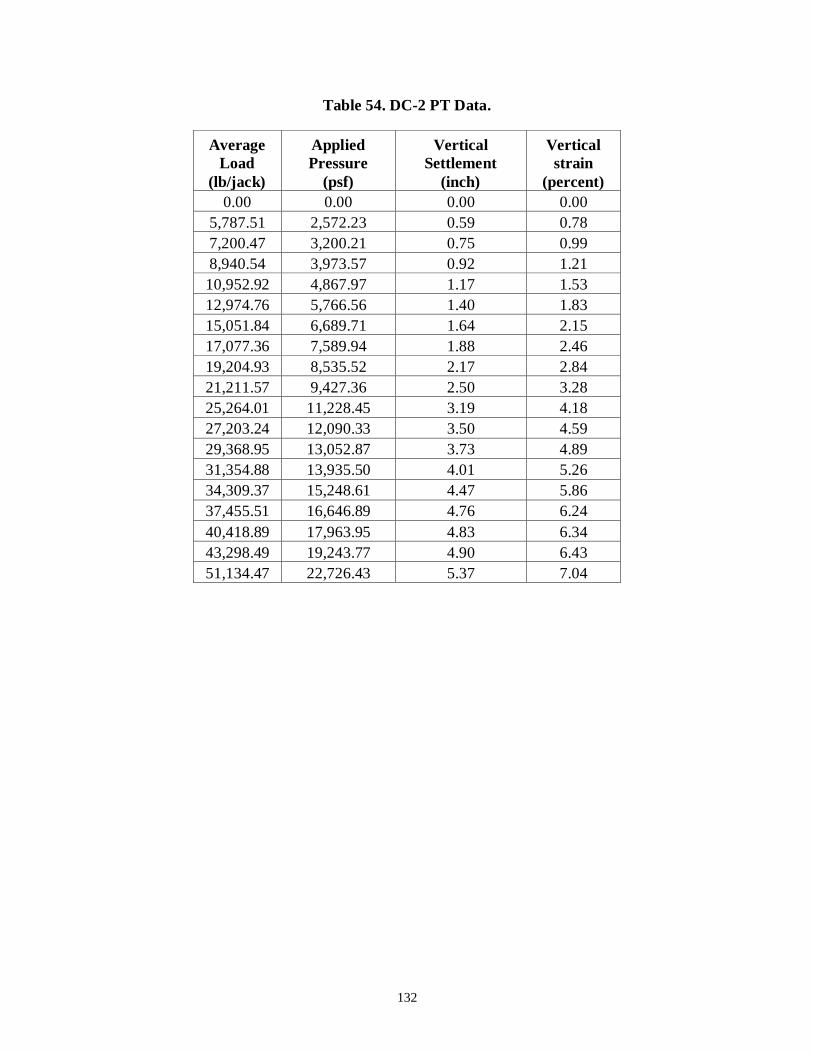
132
Table 54. DC-2 PT Data.
Average
Load
(lb/jack)
Applied
Pressure
(psf)
Vertical
Settlement
(inch)
Vertical
strain
(percent)
0.00 0.00 0.00 0.00
5,787.51 2,572.23 0.59 0.78
7,200.47 3,200.21 0.75 0.99
8,940.54 3,973.57 0.92 1.21
10,952.92 4,867.97 1.17 1.53
12,974.76 5,766.56 1.40 1.83
15,051.84 6,689.71 1.64 2.15
17,077.36 7,589.94 1.88 2.46
19,204.93 8,535.52 2.17 2.84
21,211.57 9,427.36 2.50 3.28
25,264.01 11,228.45 3.19 4.18
27,203.24 12,090.33 3.50 4.59
29,368.95 13,052.87 3.73 4.89
31,354.88 13,935.50 4.01 5.26
34,309.37 15,248.61 4.47 5.86
37,455.51 16,646.89 4.76 6.24
40,418.89 17,963.95 4.83 6.34
43,298.49 19,243.77 4.90 6.43
51,134.47 22,726.43 5.37 7.04

133
Table 55. DC-3 PT Data.
Average
Load
(lb/jack)
Applied
Pressure
(psf)
Vertical
Settlement
(inch)
Vertical
strain
(percent)
0.00 0.00 0.00 0.00
1,649.95 733.31 0.24 0.31
4,305.23 1,913.44 0.52 0.68
6,976.55 3,100.69 0.78 1.03
9,692.94 4,307.98 1.03 1.35
12,450.76 5,533.67 1.29 1.70
14,973.40 6,654.85 1.54 2.02
17,582.22 7,814.32 1.83 2.41
20,165.77 8,962.56 2.12 2.78
23,249.20 10,332.98 2.42 3.19
26,217.45 11,652.20 2.77 3.64
29,407.36 13,069.94 3.08 4.05
32,442.93 14,419.08 3.37 4.43
35,518.85 15,786.16 3.70 4.87
38,565.19 17,140.08 4.04 5.32
41,538.90 18,461.73 4.42 5.82

134
Table 56. DC-4 PT Data.
Average
Load
(lb/jack)
Applied
Pressure
(psf)
Vertical
Settlement
(inch)
Vertical
strain
(percent)
0.00 0.00 0.00 0.00
2,724.22 1,210.76 0.16 0.22
5,017.17 2,229.85 0.38 0.51
7,568.27 3,363.68 0.59 0.77
9,949.51 4,422.01 0.82 1.08
12,971.35 5,765.05 1.11 1.46
15,926.47 7,078.43 1.40 1.84
19,025.69 8,455.86 1.70 2.24
21,821.66 9,698.52 1.98 2.61
24,883.53 11,059.35 2.26 2.97
27,993.61 12,441.61 2.58 3.40
30,894.62 13,730.94 2.94 3.87
34,053.34 15,134.82 3.30 4.34
36,906.96 16,403.09 3.54 4.66
39,975.59 17,766.93 3.91 5.15
42,919.44 19,075.31 4.25 5.60
45,841.51 20,374.00 4.52 5.95
47,205.64 20,980.28 4.70 6.18
50,450.81 22,422.58 4.95 6.52
55,229.31 24,546.36 5.36 7.06
60,188.19 26,750.31 5.81 7.64

135
Table 57. DC-5 PT Data.
Average
Load
(lb/jack)
Applied
Pressure
(psf)
Vertical
Settlement
(inch)
Vertical
strain
(percent)
0.00 0.00 0.00 0.00
622.79 276.79 0.37 0.48
2,739.19 1,217.42 0.68 0.89
4,857.51 2,158.89 0.96 1.26
7,021.37 3,120.61 1.20 1.57
9,060.95 4,027.09 1.43 1.88
11,088.41 4,928.18 1.68 2.21
14,307.26 6,358.78 2.02 2.66
17,440.25 7,751.22 2.41 3.17
20,525.62 9,122.50 2.83 3.73
23,676.51 10,522.90 3.26 4.29
26,657.83 11,847.92 3.84 5.05
29,865.77 13,273.68 4.24 5.58
32,794.82 14,575.47 4.64 6.10
35,897.19 15,954.31 5.05 6.64
43,500.00 19,333.33 5.92 7.79
48,500.00 21,555.56 7.92 10.42

136
Table 58. TF-1 PT Data.
Applied
Pressure
(psf)
Vertical
Settlement
(inch)
Vertical
strain
(percent)
0.00 0.00 0.00
369.70 0.08 0.10
556.35 0.08 0.11
978.69 0.16 0.21
1,842.65 0.33 0.43
2,804.93 0.55 0.72
3,696.98 0.75 0.99
4,646.86 0.99 1.30
5,578.45 1.22 1.59
6,465.19 1.45 1.90
7,448.68 1.70 2.22
8,340.86 1.96 2.57
9,232.90 2.24 2.94
10,164.52 2.51 3.29
11,057.92 2.80 3.67
11,952.08 3.08 4.04
12,761.14 3.28 4.31
13,472.62 3.86 5.07
14,465.32 4.76 6.24
15,231.20 4.99 6.54
16,000.57 5.31 6.96
16,994.27 5.55 7.27
17,862.85 6.13 8.04
18,781.38 7.36 9.66
20,486.98 8.31 10.90

137
Table 59. TF-2 PT Data.
Applied
Pressure
(psf)
Vertical
Settlement
(inch)
Vertical
strain
(percent)
0.00 0.00 0.00
829.67 0.03 0.03
1,760.89 0.09 0.12
2,604.89 0.17 0.22
3,559.11 0.25 0.33
4,509.78 0.35 0.46
5,438.67 0.46 0.60
6,372.00 0.57 0.75
8,220.00 0.83 1.09
10,084.00 1.13 1.48
11,006.67 1.29 1.70
13,812.44 1.92 2.53
16,591.11 2.64 3.48
19,472.89 4.22 5.55
22,352.00 6.47 8.51
25,278.67 8.71 11.46
Table 60. TF-3 PT Data.
Applied
Pressure
(psf)
Vertical
Settlement
(inch)
Vertical
strain
(percent)
0.00 0.00 0.00
883.61 0.03 0.04
2,692.89 0.25 0.33
3,590.22 0.41 0.54
5,333.33 1.01 1.33
6,311.11 1.22 1.60
8,088.89 1.98 2.60
9,866.67 2.67 3.50
10,755.56 3.13 4.10
13,333.33 4.42 5.80
14,666.67 5.41 7.10
16,156.89 7.52 9.87
17,503.56 10.52 13.80

138
Table 61. TF-4 PT Data.
Applied
Pressure
(psf)
Vertical
Settlement
(inch)
Vertical
strain
(percent)
0.00 0.00 0.00
1,496.46 0.04 0.06
2,157.57 0.08 0.10
3,211.69 0.27 0.36
4,128.22 0.47 0.62
5,072.21 0.70 0.92
6,015.01 0.94 1.23
6,930.25 1.16 1.53
8,837.16 1.71 2.25
10,703.07 2.34 3.08
14,250.89 3.34 4.40

139
Table 62. TF-5 PT Data.
Applied
Pressure
(psf)
Vertical
Settlement
(inch)
Vertical
strain
(percent)
0 0 0
1,152 0.046214 0.060808
2,736 0.09353 0.123066
4,176 0.126134 0.165966
4,608 0.1733 0.228046
5,472 0.289825 0.381349
6,480 0.455363 0.599162
8,352 0.892178 1.173918
10,080 1.466227 1.929246
11,088 1.761062 2.317187
13,968 2.954815 3.887914
16,704 4.390352 5.776779
19,584 5.947989 7.826301
22,464 8.176841 10.759
25,344 9.917697 13.0496
10,944 9.843107 12.95146
0 8.705762 11.45495
0 8.700209 11.44764
2,448 0.512515 12.12201
3,744 0.663577 12.32077
5,616 0.822237 12.52953
8,496 1.007906 12.77384
11,232 1.19151 13.01542
16,992 1.785724 13.79728
22,464 3.312276 15.8059
25,920 4.924452 17.92719

140
Table 63. TF-6 PT Data.
Applied
Pressure
(psf)
Vertical
Settlement
(inch)
Vertical
strain
(percent)
0.00 0.00 0.00
889.74 0.06 0.08
1,764.73 0.20 0.27
2,522.17 0.26 0.34
3,718.49 0.38 0.50
4,546.27 0.48 0.64
5,357.84 0.65 0.85
6,255.09 0.73 0.96
8,011.64 0.93 1.22
9,850.08 1.82 2.39
13,449.91 2.27 2.99
18,706.79 3.16 4.15
21,447.16 3.68 4.84
24,041.44 4.24 5.58
26,687.14 4.76 6.27
29,321.85 5.34 7.02
30,643.85 5.79 7.62
31,937.57 6.25 8.22
33,305.27 6.83 8.99
35,809.33 7.66 10.08
38,714.79 8.76 11.52
41,250.78 10.75 14.15
43,827.56 11.95 15.73

141
Table 64. TF-7 PT Data.
Applied
Pressure
(psf)
Vertical
Settlement
(inch)
Vertical
strain
(percent)
0 0 0
906.5827 0.14 0.19
1,843.848 0.31 0.40
2,727.728 0.48 0.63
3,579.004 0.65 0.86
4,443.513 0.90 1.19
5,359.769 1.08 1.42
6,237.56 1.29 1.70
7,992.877 1.75 2.30
9,808.05 2.29 3.01
10,739.62 2.59 3.41
13,366.63 3.65 4.80
15,953.95 4.89 6.44
18,656.81 6.54 8.61
21,257.23 7.80 10.27
24,085.41 9.54 12.55
26,573.67 12.46 16.39

142
Table 65. TF-8 PT Data.
Applied
Pressure
(psf)
Vertical
Settlement
(inch)
Vertical
strain
(percent)
0.00 0.00 0.00
901.25 0.19 0.24
1,784.19 0.39 0.51
2,673.33 0.60 0.78
3,610.08 0.81 1.07
4,460.27 1.00 1.32
5,317.64 1.20 1.58
6,194.72 1.42 1.87
7,942.55 1.87 2.46
9,762.13 2.38 3.13
10,636.89 2.66 3.50
13,345.60 3.62 4.76
16,003.43 4.70 6.18
18,547.61 5.90 7.76
21,274.89 7.35 9.67
23,999.31 8.62 11.34
26,608.37 10.10 13.29
29,178.74 13.51 17.77

143
Table 66. TF-9 PT Data.
Applied
Pressure
(psf)
Vertical
Settlement
(inch)
Vertical
strain
(percent)
0.00 0.00 0.00
434.85 0.06 0.08
573.32 0.07 0.09
746.42 0.09 0.12
1,225.31 0.14 0.19
1,898.80 0.24 0.31
2,541.19 0.32 0.42
3,146.98 0.41 0.54
3,725.78 0.50 0.65
4,334.89 0.63 0.84
5,585.85 0.85 1.12
6,790.22 1.08 1.43
7,433.04 1.24 1.63
9,292.90 1.74 2.29
11,195.61 2.46 3.24
13,072.80 3.36 4.43
14,953.66 5.17 6.80
16,806.30 6.49 8.53
18,680.80 8.05 10.59
20,537.79 9.95 13.09
22,360.24 11.83 15.56

144
Table 67. TF-10 PT Data.
Applied
Pressure
(psf)
Vertical
Settlement
(inch)
Vertical
strain
(percent)
0.00 0.00 0.00
375.25 0.09 0.12
1,115.40 0.28 0.37
1,443.58 0.35 0.46
1,641.11 0.39 0.51
2,060.36 0.50 0.66
2,478.58 0.64 0.84
2,915.38 0.77 1.02
3,691.10 1.07 1.40
4,536.46 1.46 1.92
4,958.59 1.68 2.22
6,186.24 2.53 3.33
7,432.09 3.86 5.08
8,625.99 6.32 8.32
8,838.17 9.05 11.91
10,339.14 10.85 14.28
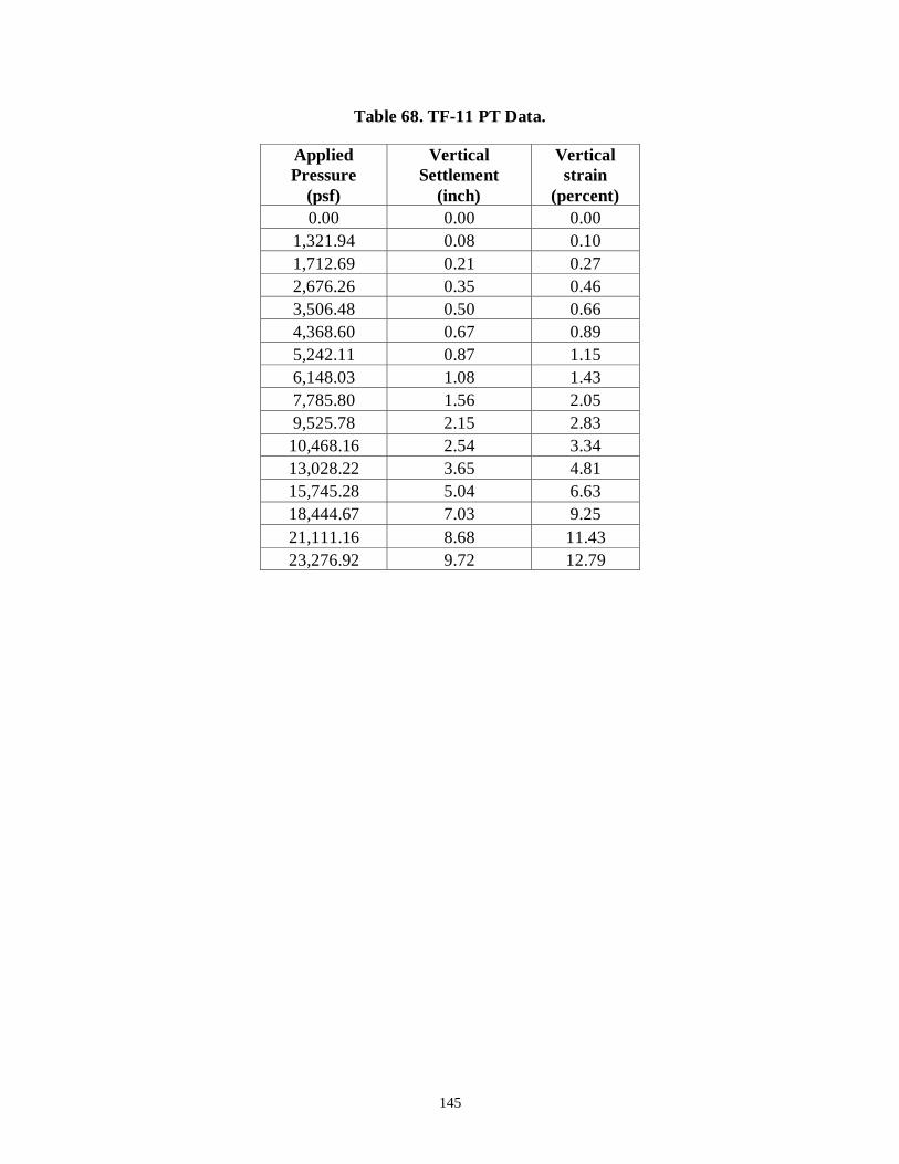
145
Table 68. TF-11 PT Data.
Applied
Pressure
(psf)
Vertical
Settlement
(inch)
Vertical
strain
(percent)
0.00 0.00 0.00
1,321.94 0.08 0.10
1,712.69 0.21 0.27
2,676.26 0.35 0.46
3,506.48 0.50 0.66
4,368.60 0.67 0.89
5,242.11 0.87 1.15
6,148.03 1.08 1.43
7,785.80 1.56 2.05
9,525.78 2.15 2.83
10,468.16 2.54 3.34
13,028.22 3.65 4.81
15,745.28 5.04 6.63
18,444.67 7.03 9.25
21,111.16 8.68 11.43
23,276.92 9.72 12.79
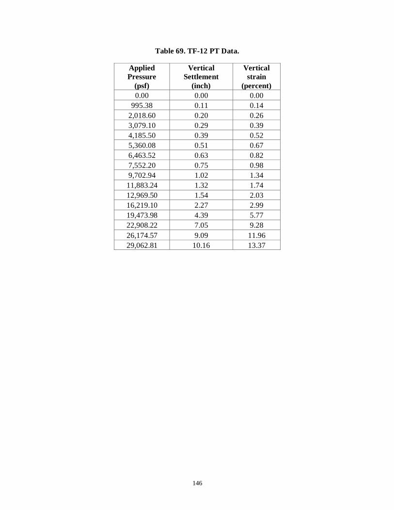
146
Table 69. TF-12 PT Data.
Applied
Pressure
(psf)
Vertical
Settlement
(inch)
Vertical
strain
(percent)
0.00 0.00 0.00
995.38 0.11 0.14
2,018.60 0.20 0.26
3,079.10 0.29 0.39
4,185.50 0.39 0.52
5,360.08 0.51 0.67
6,463.52 0.63 0.82
7,552.20 0.75 0.98
9,702.94 1.02 1.34
11,883.24 1.32 1.74
12,969.50 1.54 2.03
16,219.10 2.27 2.99
19,473.98 4.39 5.77
22,908.22 7.05 9.28
26,174.57 9.09 11.96
29,062.81 10.16 13.37
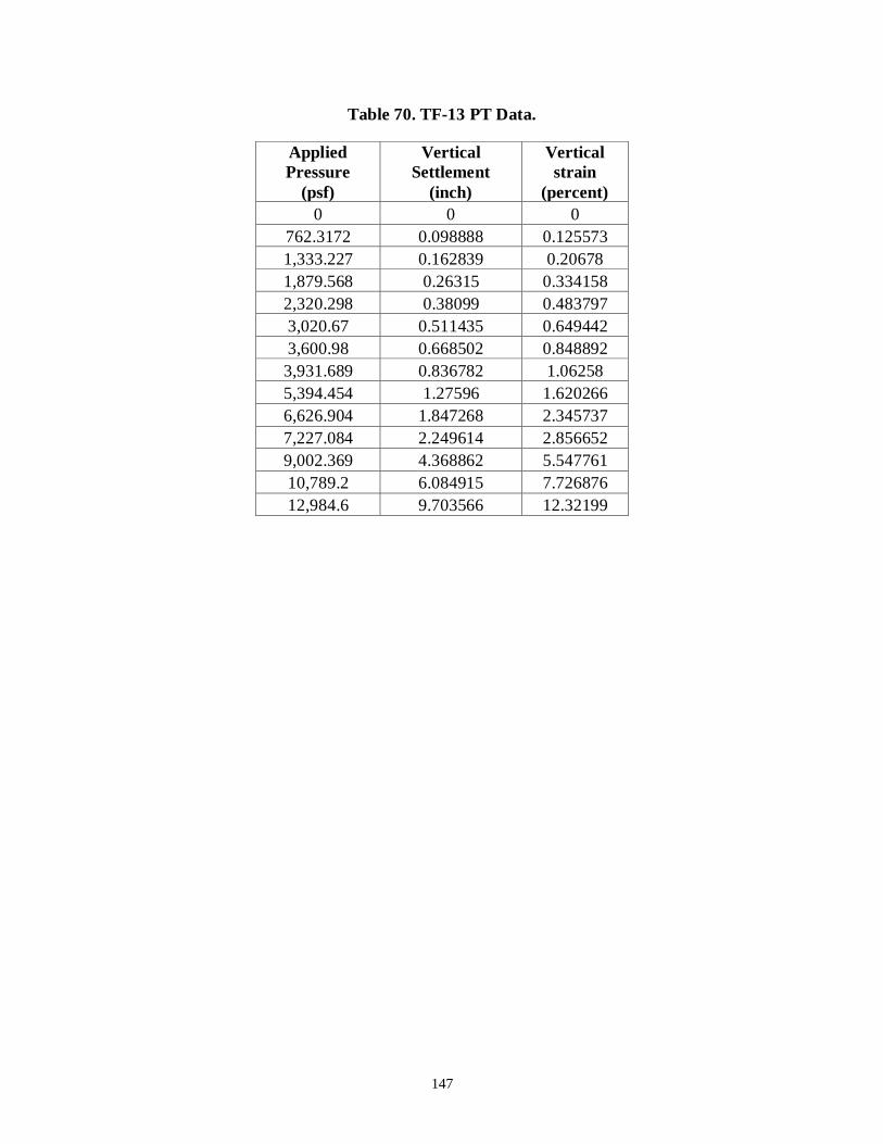
147
Table 70. TF-13 PT Data.
Applied
Pressure
(psf)
Vertical
Settlement
(inch)
Vertical
strain
(percent)
0 0 0
762.3172 0.098888 0.125573
1,333.227 0.162839 0.20678
1,879.568 0.26315 0.334158
2,320.298 0.38099 0.483797
3,020.67 0.511435 0.649442
3,600.98 0.668502 0.848892
3,931.689 0.836782 1.06258
5,394.454 1.27596 1.620266
6,626.904 1.847268 2.345737
7,227.084 2.249614 2.856652
9,002.369 4.368862 5.547761
10,789.2 6.084915 7.726876
12,984.6 9.703566 12.32199

148
Table 71. TF-14 PT Data.
Applied
Pressure
(psf)
Vertical
Settlement
(inch)
Vertical
strain
(percent)
0.00 0.00 0.00
580.06 0.16 0.21
1,191.94 0.25 0.32
1,829.39 0.35 0.46
2,466.98 0.45 0.59
3,001.13 0.54 0.71
3,611.30 0.64 0.84
4,225.24 0.74 0.98
5,402.42 0.94 1.24
6,620.61 1.15 1.51
7,233.56 1.28 1.68
9,042.58 1.65 2.18
10,965.38 2.07 2.72
12,738.15 2.53 3.33
14,571.33 3.08 4.05
16,460.84 3.68 4.84
18,314.54 4.45 5.85
20,140.13 5.51 7.25
22,071.79 7.13 9.39
23,603.11 9.65 12.69

149
ACKNOWLEGEMENTS
The authors would like to acknowledge the hard work and effort of Ms. Jan Li, Mr. Moustafa
Ibrahim-Awad, Mr. Tim Tuggle, Mr. Jeffrey Lin, and Mr. Daniel Powers in helping to construct
and test the performance tests at Turner-Fairbank Highway Research Center. In addition, thanks
to Dr. Fassil Beshah for coordinating use of the Structures Laboratory. For the tests conducted in
Defiance County, OH, the authors wish to thank Mr. Warren Schlatter and Mr. Jeff Timbrook,
along with the participants of each GRS EDC Validation Session. Finally, the authors would also
like to extend their appreciation for the technical review comments prepared by (in alphabetical
order) Mr. Daniel Alzamora of the Resource Center, Khalid Mohamed of the Office of Bridge
Technology, and Dr. Justin Ocel of the Office of Infrastructure Research and Development.


151
REFERENCES
1. Adams, M., Nicks, J., Stabile, T., Wu, J., Schlatter, W., and Hartmann, J., “Geosynthetic
Reinforced Soil Integrated Bridge System Interim Implementation Guide”. Report, FHWA-
HRT-11-026, Federal Highway Administration, McLean, VA, 2011a.
2. Adams, M.T., Lillis, C.P., Wu, J.T.H., and Ketchart, K., “Vegas Mini Pier Experiment and
Postulate of Zero Volume Change,” Proceedings, Seventh International Conference on
Geosynthetics, Nice, France, 2002, pp. 389–394.
3. ASTM D7181, “Standard Test Method for Consolidated Drained Triaxial Compression Test
for Soils,” Annual Book of ASTM Standards, ASTM International, West Conshohocken, PA,
2011.
4. Adams, M.T., Ketchart, K., and Wu, J.T.H., “Mini Pier Experiments: Geosynthetic
Reinforcement Spacing and Strength as Related to Performance,” Geotechnical Special
Publication 165, Geosynthetics in Reinforcement and Hydraulic Applications, Geo-Denver
2007, ASCE, Denver, CO, 2007.
5. Adams, M., Nicks, J., Stabile, T., Wu, J., Schlatter, W., and Hartmann, J., “Geosynthetic
Reinforced Soil Integrated Bridge System Synthesis Report,” Report, FHWA-HRT-11-027,
Federal Highway Administration, McLean, VA, 2011b.
6. Juran, I., Guermazi, A., Chen, C.L. and Ider, M.H., “Modeling and simulation of load
transfer in reinforced soils: Part 1”. International Journal for Numerical and Analytical
Methods in Geomechanics, 12(2), John Wiley and Sons, 2005, pp. 141–155.
7. Ketchart, K. and Wu, J.T.H. “Performance Test for Geosynthetic-Reinforced Soil including
Effects of Preloading,” Report, FHWA-RD-01-018, Federal Highway Administration,
McLean, VA, 2001. <http://www.tfhrc.gov/structur/gtr/01-018.pdf>, retrieved on December
6, 2012.
8. Elton, D.J. and Patawaran, M.A.B., “Mechanically Stabilized Earth (MSE) Reinforcement
Tensile Strength from Tests of Geotextile Reinforced Soil,” Technical Report, Alabama
Highway Research Center, Auburn University, Auburn, AL, 2005.
9. Wu, J.T.H., Adams, M., Pham, T.Q., Lee, S.H., and Ma, C.Y., “A generic soil-geosynthetic
composite test,” International Journal of Geotechnical Engineering, 6(1), 2012,
pp. 103–116.
10. AASHTO, “LRFD Bridge Design Specifications, Edition 5,” Report, American Association
of State Highway and Transportation Officials, Washington, DC, 2012.
11. Wu, J.T.H., Pham, T.Q., and Adams, M.T., “Composite Behavior of Geosynthetic-
Reinforced Soil (GRS) Mass,” Report, FHWA-HRT-10-077, Federal Highway
Administration, McLean, VA, 2010.
12. Wu, J.T.H. and Pham. T.Q., “Load-Carrying Capacity and Required Reinforcement Strength
of Closely-Spaced Soil-Geosynthetic Composites,” ASCE Journal of Geotechnical and
Geoenvironmental Engineering, 139(1), Reston, VA, 2013.
13. ASTM D3080, “Standard Test Method for DIRECT Shear Test of Soils Under Consolidated
Drained Conditions,” Annual Book of ASTM Standards, ASTM International, West
Conshohocken, PA, 2004.
14. ASTM D4595, “Standard Test Method for Tensile Properties of Geotextiles by the Wide-
Width Strip Method,” Annual Book of ASTM Standards, Vol. 4.13, ASTM International,
West Conshohocken, PA, 2006, pp. 40–50.
15. AASHTO T-99, “Standard test methods for moisture density relations of soils and soil
aggregate mixtures using 5.5 lb rammer and 12 in. drop. Standard specifications for highway

152
materials and methods of sampling and testing,” American Association of State Highway
Transportation Officials, Washington, DC, 2011.
16. ASTM D4253, “Standard Test Methods for Maximum Index Density and Unit Weight of
Soils Using a Vibratory Table,” Annual Book of ASTM Standards, ASTM International, West
Conshohocken, PA, 2000.
17. Industrial Fabrics, “Geotext 200 ST Product Data Sheet,” < http://www.ind-
fab.com/downloads/200st.pdf>, retrieved on December 6, 2012.
18. Propex, “Geotex Woven Geotextiles Product Information,”
<http://geotextile.com/product/geotex.html>, retrieved on December 6, 2012.
19. US Fabrics, “US 3600/3600 Product Information,”
<http://www.usfabricsinc.com/products/us-3600-3600>, retrieved on December 6, 2012.
20. ASTM D4632, “Standard Test Method for Grab Breaking Load and Elongation of
Geotextiles, Annual Book of ASTM Standards,” ASTM International, West Conshohocken,
PA, 2008.
21. Briaud J.-L., “Introduction to Soil Moduli,” Geotechnical News, June 2001, BiTech
Publishers Ltd, Richmond, BC, Canada, 2001. ([email protected]).
22. Adams, M.T., “Performance of a Prestrained Geosynthetic-Reinforced Soil Bridge Pier,”
International Symposium on Mechanically Stabilized Backfill, Wu, J.T.H. (ed), Denver,
Balkema, 1997, pp. 35–53.
23. Wu, J.T.J., Ketchart, K., and Adams, M. “GRS Bridge Piers and Abutments,” FHWA
Research Report, FHWA-RD-00-038, FHWA, McLean, VA, 2000.
24. Meyerhof, G.G., “The ultimate capacity of foundations on slopes,” Procs., 4th Int. Conf. on
Soil Mechanics and Found. Engrg., London, August, London, England, 1957, pp. 384–386.
25. Pham, T.Q., “Investigating Composite Behavior of Geosynthetic Reinforced Soil (GRS)
Mass,” Ph.D. Thesis, University of Colorado, Denver CO, 2009.
26. NAVFAC, “Soil Mechanics Design Manual 7.01,” Naval Facilities Engineering Command,
Alexandria, VA, 1986.
27. Gibson, R.E., “Some results concerning displacements and stresses in a non-homogeneous
elastic half space,” Geotechnique, Vol. 17, 1967, pp. 58–67.
28. Poulos, H.G. and Davis, E.H., “Elastic Solutions for Soil and Rock Mechanics,” John Wiley
and Sons, New York, 1974.
29. Samtani, N.C., Nowatzki, E.A., and Mertz, D.R., “Selection of Spread Footings on Soils to
Support Highway Bridge Structures,” Report, FHWA-RC/TD-10-001, FHWA Resource
Center, Matteson, IL, 2010.
30. Nicks, J.E., Adams, M., Wu, J., “A new approach to the design of closely spaced
geosynthetic reinforced soil for load bearing applications,” TRB Annual Compendium of
Papers, Transportation Research Board, Washington DC., 2013a.
31. VanBuskirk, C.D., “Adoption and Implementation of GRS design concepts,” 19th
Vancouver
Geotechnical Society Symposium, Vancouver Geotechnical Society, Vancouver, Canada,
2010.
32. Nicks, J.E., Adams, M.T., and Alzamora, D.A., “Implications of MSE Connection Criteria
for Frictionally Connected GRS Structures,” Proceedings of Geosynthetics 2013, Long
Beach, CA, 2013b.
33. Wu, J.T.H., Lee, K.Z.Z., Helwany, S.B., and Ketchart, K., “Design and Construction
Guidelines for GRS Bridge Abutment with a Flexible Facing,” Report, No. 556, National
Cooperative Highway Research Program, Washington, DC, 2006.

153
34. Bathurst, R.J. and Benjamin, D.J., “Failure of a Geogrid-Reinforced Soil Wall,” Report,
Transportation Research Board, Washington, DC, 1990, pp. 109–116.
35. Barker, R.M., Duncan, J.M., Rojiani, K.B., Ooi, P.S.K., Tan, C.K., and Kim, S.G., “Manuals
for the Design of Bridge Foundations,” NCHRP Report 343, Transportation Research Board,
Washington, DC, 1991.
36. Paikowsky, S.G., Canniff, M.C., Lesny, K., Kisse, A., Amatya, S., and Muganga, R., “LRFD
design and construction of shallow foundations for highway bridges,” NCHRP Report 651,
Transportation Research Board, Washington DC, 2010.
37. Kulicki, J.M., Prucz, Z., Clancy, C.M., Mertz, D.R., and Nowak, A.S., “Final Report for
NCHRP Project 20-7/186: Updating the Calibration Report for AASHTO LRFD Code,”
Report, Transportation Research Board, Washington, DC., 2007
38. Benjamin, C.V.S., Bueno, B.S., Lodi, P.C. and Zornberg, J.G., “Installation and ultraviolet
exposure of geotextiles,” Fourth European Geosynthetics Conference, EuroGeo4,
Edinburgh, United Kingdom, 8–10 September, 2008, pp. 18.
39. Grouni, H.N. and Nowak, A.S., “Calibration of the Ontario Bridge Design Code 1983
Edition,” Canadian Journal of Civil Engrg. 11(4), 1984: pp. 760–770
40. Paikowsky, S. G., with contributions from Birgisson, B., McVay, M., Nguyen, T., Kuo, C.,
Baecher, G., Ayyab, B., Stenersen, K., O’Malley, K., Chernauskas, L., and O’Neill, M. ,
“Load and Resistance Factor Design (LRFD) for Deep Foundations, NCHRP (Final) Report
507,” Report, Transportation Research Board, Washington, DC, 2004.
41. Bathurst, R.J., Allen, T.M., and Nowak, A.S., “Calibration concepts for load and resistance
factor design (LRFD) of reinforced soil walls,” Canadian Geotechnical Journal, NRC
Canada, Volume 45, 2008, pp. 1,377–1,392.

HRDi-40/08-13(WEB)E