Ann. Rev. Fluid Mech. 1979. 11 :401-41 Copyright © by Annual Reviews Inc. All rights reserved

GEOSTROPHIC TURBULENCE x8147

Peter B. Rhines Woods Hole Oceanographic Institution, Woods Hole, Massachusetts 02543

1 INTRODUCTION AND EQUATIONS

Geostrophic turbulence is the chaotic, nonlinear motion of fluids that are near to a state of geostrophic and hydrostatic balance. Thus, f xu c::: -Vpjp-g, where f is twice the component of the planetary rotation vector, n, in the local vertical direction, parallel to g, which is the acceleration due to gravity, plus the mean centrifugal effect of n. Pressure is denoted by p; u is velocity; and p is density. This balance occurs at time scales greater than a day, and length scales greater than tens of kilometers (for the Earth's oceans) or hundreds of kilometers (for the atmosphere). More specifically, we require that the Ekman number (E == vlf H2), the Rossby number (Ro == U j f L), and the nondimensional frequency [(fT)- 1] each be small. U is a representative fluid velocity, L is its horizontal length scale, H its vertical length scale, T its time scale, and v is the kinematic viscosity.

The geostrophic-balance equation is a singular perturbation with respect to neglected accelerations and frictional forces. The curl of the full momentum equation is unaffected by the dominant part of the pressure force and gives a fully predictive potential vorticity equation,

Dq = forcing - dissipation + O(Ro). (1.1)

Dt

Here, q is the potential vorticity, defined in several forms below, and D / Dt = a/at + u . V is the Lagrangian acceleration. The derivation of the vorticity equations appropriate to a spherical planet is a lengthy process ; here we take them as given. The dominant small parameters are Ro, the fluid depth/planetary radius, the aspect ratio of the motion, H/L, and the ratio of Corio lis to buoyancy forces,f/N (where N2 = (-g/p)op/oz) [see, for example, Phillips (1963), Miles ( 1974), and Grimshaw (1975)] .

A useful form of (1.1) (not restricted to geostrophic flow) has

q = ql = (Vxu+2Q)· Vp/p,

0066·4189/79/01 15.0401$01.00

(1.2)

401

Ann

u. R

ev. F

luid

Mec

h. 1

979.

11:4

01-4

41. D

ownl

oade

d fr

om w

ww

.ann

ualr

evie

ws.

org

by C

alif

orni

a In

stitu

te o

f T

echn

olog

y on

11/

06/1

2. F

or p

erso

nal u

se o

nly.

402 RHINES

where p is the incompressible density (Ertel 1942) and ql is the component of absolute vorticity normal to density surfaces, multiplied by the inverse separation between adjacent surfaces. In this direction, the twisting due to buoyancy, Vp x V P -1, has no direct effect. Equation ( 1.2) is equivalent to Kelvin's circulation theorem written for a material circuit lying on an isopycnal (constant-density) surface.

Scaled for Boussinesq, quasi-geostrophic flow, (1.1) involves a potential vorticity

2 a [N at/!] N at/! Q=Q2= V t/!+az N2 oz + (3y-[t5(z)-t5(z+H)]

N2 GZ

+ (j(z+ H)/oh* ; D/Dt = %t+o(l/I, )/a (x, y), (1.3)

1 = 10 + t1y, u = (-aljJ/oy,ot/!/ox), h = H -h*(x,y), v2 = a2/ox2+02/ay2,

where ljJ is a stream function for the horizontal velocity (nondivergent to order Ro). Vertical velocity is dynamically significant, however, and works through the stretching of planetary vorticity (second term). The spherical geometry is approximated by linear dependence of f on y (x and yare east-west and north-south Cartesian coordinates). The delta functions account for the intersection of isopycnal surfaces with the top and bottom boundaries, which lie at z = 0 and z = -h = - H + h*(x,y).

Thus qz contains flow-dependent terms, the vertical vorticity and vortex stretching, and also environmental effects, such as the shape and mean rotation of the bounding planet.

The continuously stratified fluid can be approximated by a series of constant-density layers, for which (in the ith layer)

hi = '1i+ 1-'1i+Hi, PH 1 - Pi = gllpi11i (1.4)

Here, 11i is the perturbed height of the ith interface, analogous to ( -f/ N2)onoz.

Much of the classical theory for large-scale circulations applies simpli­fied forms of (1.1) with specified forcing and laminar friction. The good­ness of the theories depends upon the accuracy of the potential vorticity principle and also upon the strength of eddy transports subsumed by (1.1), but neglected in the theory. It is very unlikely that a strongly turbulent fluid can be understood, even in the mean, until the nature of its energy-containing eddies is rationalized.

Conservation of this single scalar potential vorticity puts powerful constraints on the flow. It suggests that knowledge of the deformation

Ann

u. R

ev. F

luid

Mec

h. 1

979.

11:4

01-4

41. D

ownl

oade

d fr

om w

ww

.ann

ualr

evie

ws.

org

by C

alif

orni

a In

stitu

te o

f T

echn

olog

y on

11/

06/1

2. F

or p

erso

nal u

se o

nly.

GEOSTROPHIC TURBULENCE 403

of material surfaces may give information about the dynamics. Conserva­tion of q following the fluid has motivated exact solutions to nonlinear evolution problems; for example, the theory of formation of fronts (Hoskins & Bretherton 1972 ).

The qualitative properties of geostrophic turbulence that most concern us here are:

1 . the ability of chaotic flow to extend contours of constant q, hence cascading q to small scale;

2. the inhibition of this cascade by large-scale environmental fields of q [say, given by Q(x)];

3. the enhancement of the cascade by small-scale environmental varia­tions in Q; and

4. the ability of turbulence to transport potential vorticity systematically down its mean gradient, VQ. Together, these events decide the sense of evolution of the energy­

containing eddies, the balance between turbulence and wave motion, the cOllversion between potential and kinetic energy, the nature of time­or ensemble-mean circulations generated along geostrophic (Q =

constant) contours (when the contours are closed), and the mean circula­tion driven across Q contours (when they are blocked by lateral boundaries ).

As one piece of evidence for the presence of mesoscale turbulence, Figure 1 shows a NOAA satellite photograph of the sea-surface tem­perature in the western North Atlantic. The 0(100 km)-wide eddies are of the same size as the Gulf Stream that spawned them, yet are much smaller than either the ocean basin or the broadest components of the wind-driven circulation.

Because of the steeply decreasing spectral energy with increasing wave number, geostrophic turbulence tends, by nature, to be very dependent on the details of the energy-containing eddies, and the forcing effects that created them. A vast range of particular flow problems is relevant to the subject, but we will be constrained here to describe only a few of these.

2 TWO-DIMENSIONAL TURBULENCE

The prototype for geostrophic eddy fields is the motion of uniform­density, incompressible fluid in two dimensions. The original geophysical motivations for this study (that the atmosphere is essentially two­dimensional and weakly dissipative of energy) turn out not to be true, but many of the phenomena of geostrophic turbulence find expression

Ann

u. R

ev. F

luid

Mec

h. 1

979.

11:4

01-4

41. D

ownl

oade

d fr

om w

ww

.ann

ualr

evie

ws.

org

by C

alif

orni

a In

stitu

te o

f T

echn

olog

y on

11/

06/1

2. F

or p

erso

nal u

se o

nly.

Figure 1 A sea-surface temperature photograph of the Gulf Stream leaving Cape Hatteras. Darker shades represent warmer water. This front between polar and subtropical water regularly produces geostrophic eddies. Courtesy of NOAA Environmental Satellite Service.

R :<:I ::I: Z !}l

Ann

u. R

ev. F

luid

Mec

h. 1

979.

11:4

01-4

41. D

ownl

oade

d fr

om w

ww

.ann

ualr

evie

ws.

org

by C

alif

orni

a In

stitu

te o

f T

echn

olog

y on

11/

06/1

2. F

or p

erso

nal u

se o

nly.

GEOSTROPHIC TURBULENCE 405

in two-dimensional turbulence. Without this kinship, two-dimensional turbulence would be of less interest, a kind of stochastic complement to 19th century hydrodynamics.

With q == (, the potential vorticity equation is

aV2ljJ + 8(ljJ, V2ljJ) vV4ljJ _ RV2ljJ at a(x,y)

( = V2ljJ, U = ( -��, ��). (2. 1 )

where v i s the kinematic viscosity and R the Ekman drag at the lower boundary, R = (v/ f H2)1/2 = E l/2! Define e(k) dk to be the kinetic energy, � 1 VljJ 12, contained in Fourier components with wave numbers 1 k 1 between k and k+dk. Then (2.1) yields energy and enstrophy (= squared vorticity /2) equations

:t f e dk = -2v f k2 e dk -2R f e dk < 0,

:t f Pe dk = -2v f k4e dk-2R f k2e dk < O. (2.2)

Taylor (1917) established that the many-fold stretching of vortex lines is necessary to the cascade of energy from finite scales to small; with the vortex stretching term � . Vu = 0 identically, hence the energy dissipa­tion � 0 with v. For a finite initial scale of motion, the right sides of (2.2) both vanish for finite time, leaving conservation of total energy and enstrophy (i.e. i squared vorticity), a/at flO dk = a/ot fk2e dk = 0.

Imagine an initial-value problem in which energy occupies a narrow band of wave numbers. It is most plausible that inertial interactions will cause a spread of energy to adjacent wave numbers. Suppose that this spreading is characterized by growth of the dispersion of e(k) (about its center), i.e.

where k� = fk"e dk/fe dk. With the conservation equations, this gives

ok1 k4 2 at < -2(v 4+Rk2) < O.

The first moment of e moves to a smaller wave number, and finite values of v and R merely hasten the expansion in scale. The overwhelming

Ann

u. R

ev. F

luid

Mec

h. 1

979.

11:4

01-4

41. D

ownl

oade

d fr

om w

ww

.ann

ualr

evie

ws.

org

by C

alif

orni

a In

stitu

te o

f T

echn

olog

y on

11/

06/1

2. F

or p

erso

nal u

se o

nly.

406 RHINES

Figure 2 Contours of constant vorticity in a barotropic, two-dimensional turbulence experiment. The extension of the initially roundish patterns is evident. The model has 1282 degrees of freedom.

control of the ens trophy invariant prevents an energy cascade to the right. Visualize the problem of redistributing a fixed mass (of density e) lying initially at k = kO, while conserving its moment of inertia about

k = O. No more than one fourth of the mass can be moved tok = 2ko for, to balance, all of the the remainder milst be shifted back to k = 0 [see Batchelor ( 1953), Fjprtoft (1953), and Merilees & Warn ( 1975) for further detail] . 1

These events are accompanied by the distortion in physical space of vorticity contours by the shear of larger-scale eddies (Figure 2). If these q contours behave like typical, marked fluid surfaces, then it is

1 Two-dimensional turbulence in a real fluid requires stabilization against three­dimensional disturbances. Strong planetary rotation (f) will do so, but at the same time transmits frictional influence from horizontal boundaries to the interior fluid. In practice, two-dimensional turbulence often decays in energy more rapidly than three-dimensional turbulence (if E'/2 > Ro) (Ibbetson & Tritton 1 975).

Ann

u. R

ev. F

luid

Mec

h. 1

979.

11:4

01-4

41. D

ownl

oade

d fr

om w

ww

.ann

ualr

evie

ws.

org

by C

alif

orni

a In

stitu

te o

f T

echn

olog

y on

11/

06/1

2. F

or p

erso

nal u

se o

nly.

GEOSTROPHIC TURBULENCE 407

inescapable that, on average, they should increase in length with time. A proof [that «<5xt)p) � (<5xo)P for any positive p, where <5xt is an infinites­imal separation distance between two fluid particles in an isotropic turbulence field and < > is an ensemble mean] is given by Cocke (1969) and Orszag (1970a). An exponential growth of the length of a q contour with time is suggested within an inertial range (Batchelor & Townsend 1959).

In an incompressible fluid the stretching of q contours requires an increase in the average gradient of q, in direct proportion. This measure of the scale of the vorticity field thus decreases [specifically, (iJ/Ot)k4 > OJ. The enstrophy dissipates in proportion to the squared vorticity gradient; its enhancement by stretching of q contours is analogous to energy­dissipation enhancement by vortex stretching in three dimensions [Kraichnan (1967), Batchelor ( 1969), Lilly ( 197 1)] . The opposing energy and enstrophy cascades (with kl decreasing, k4 increasing, ko and k2 remaining nearly constant) cause streamline (t/J) patterns to grow in scale while vorticity is strained into thin filaments [visualize the static deformation, t/J, of a membrane loaded with a circular weight, q, and then by an elongated load of the same weight ('\12t{! = q)]. Figure 3 shows a typical realization of freely-evolving two-dimensional turbulence, using a 1282 Fourier-mode numerical code developed by Orszag (e.g. Herring et al 1974).

The greatest weakness in these arguments for the two-dimensional turbulence cascade is that vorticity contours are, in fact, special, and are related to the motion that distorts them. Isotropic velocity fields can be found that will cause the cascade to run backward (for instance, artificially reverse the velocity field in a realization of inviscid two­dimensional turbulence). Cocke's result, that line segments are stretching on average with the turbulence running either backward or forward, suggests that the meticulous unwinding of vorticity contours is indeed unlikely.

Below, I introduce geophysical effects that defeat the ens trophy cascade by organizing the q contours. With two-dimensional turbulence, however, the back effect of the strained small-scales on the larger, actively straining eddies can be estimated. The sense of the energy exchange is indicated by heuristic arguments familiar to atmospheric studies (e.g. Starr 1953). Small eddies, if distorted by larger eddies in the "obvious" sense of a passive dye trace, develop Reynolds stress patterns tending to feed energy to the larger scale. The transfer from cyclones to the zonal-average winds in the atmosphere is thought to be an example, although we shall see that several other wave number cascades are active in such a fluid.

Ann

u. R

ev. F

luid

Mec

h. 1

979.

11:4

01-4

41. D

ownl

oade

d fr

om w

ww

.ann

ualr

evie

ws.

org

by C

alif

orni

a In

stitu

te o

f T

echn

olog

y on

11/

06/1

2. F

or p

erso

nal u

se o

nly.

408 RHINES

Thus, as vorticity patterns are teased out by the shearing of larger eddies, their characteristic wave number k increases, while their vorticity content per octave of wave numbers (�k3a roughly) remains nearly constant. Hence the energy content in this same band ( '" ka) tends to decrease in time. However, the magnitude of this energy transfer becomes small as the disparity in scale increases between strained and straining eddies. The velocity induced back at large scale becomes slight, due to cancellation among closely packed positive and negative vortex elements. For a rough quantitative estimate, let the ratio of energy densities of the two scales be lif!V�, which is large if wave number k � p. The charac­teristic transfer time is just the inverse strain rate (or circulation time)

T

200 DAYS

o x

2000 KM

Figure 3 Time-longitude diagram for rjI showing the evolution of the scale of the eddies along a single latitude in the periodic box. Time increases downward. The Galerkin treatment of the nonlinear terms was developed, for this model, by Orszag (see Herring et al 1974). Geophysical models were developed by Rhines (1977).

Ann

u. R

ev. F

luid

Mec

h. 1

979.

11:4

01-4

41. D

ownl

oade

d fr

om w

ww

.ann

ualr

evie

ws.

org

by C

alif

orni

a In

stitu

te o

f T

echn

olog

y on

11/

06/1

2. F

or p

erso

nal u

se o

nly.

GEOSTROPHIC TURBULENCE 409

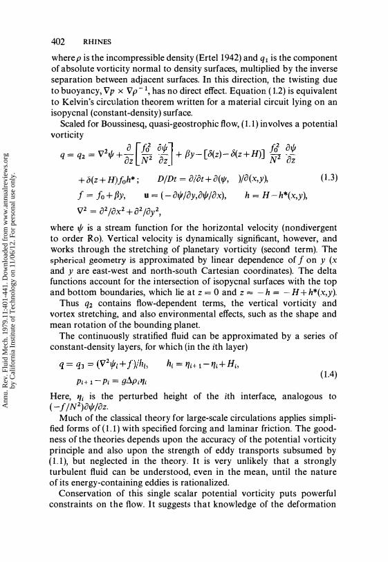
of the bigger eddies [ ",-,(kVk)-l]. During that time the energy transferred ("'v�) is a small fraction of the energy already present. Kraichnan ( 1975) discusses these events in more detail.

Point Vortices and Thermal Equilibrium Solutions

Methods of equilibrium statistical mechanics have been applied to in viscid two-dimensional turbulence for the idealized case of a fluid with a finite number of degrees of freedom: ensembles of point vortices [e.g. Onsagar ( 1949), Kraichnan ( 1975), Pointin & Lundgren (1977)J and artificially truncated sets of Fourier modes [Kraichnan (1967, · 1975), Salmon et al (1976)].

Point vortices, ljJ = I. Ai In fi, where fi is the radial distance to the center of the ith vortex, move about physical space subject to a Hamiltonian,

H = �(2n)-lp L AAj In (fij/fO), i> j

where Ai is the circulation about the ith vortex, rij is the distance between ith and jth vortices, and fO is an arbitrary constant. The equations of motion are

dxddt = oH/o'}!;, dYddt = - oR/ox;,

where (X;,Yi) == (Xi,Yi) (pAir 1/2 are the coordinates of the ith vortex. The equilibrium behavior is found [Kraichnan (1975)J to resemble that of a continuous vorticity distribution, truncated at some uppermost wave number. The cascade of energy in two-dimensional turbulence to large scale has been likened to the negative-temperature equilibria of point vortices, which involve clustering of vortices of like sign. But, the actual continuum cascade involves, rather, increasingly fine-grained vorticity and coarse�grained velocity. Straightforward segregation of the vortices by sign cannot occur regularly, because it would involve an increase in kinetic energy. Charney (1960) generalizes point vortices to a stratified fluid.

For continuous vorticity distributions, the inviscid, truncated Fourier system lies on the intersection of a hypersphere (E = constant) and a hyper-ellipse (k�E = constant) in a phase space whose coordinates are the respective F ouder amplitudes. Assuming equal probability for each permitted state, we find a micro-canonical (specified E and k�E) prob­ability distribution for energy and enstrophy. This approximates a Boltzmann distribution provided that the energy is not concentrated in a few modes:

&k(Xk) = n- 112«()(+ �k2)112 exp ( - ()(Ek - f3Zk)'

Ann

u. R

ev. F

luid

Mec

h. 1

979.

11:4

01-4

41. D

ownl

oade

d fr

om w

ww

.ann

ualr

evie

ws.

org

by C

alif

orni

a In

stitu

te o

f T

echn

olog

y on

11/

06/1

2. F

or p

erso

nal u

se o

nly.

410 RHINES

Ek,Zk are the energy and enstrophy at discrete wave number k. If the lowest few wave numbers are not significantly energetic, the energy spectrum is

8(k) = ink(oc+ 13k2)� 1.

It is plausible that transient, dissipative cascades proceed in the direction of thermal equilibrium. For initial conditions corresponding to a peak of energy at intermediate k, with an increasingly dense set of wave numbers present, oc and 13 are both positive. The corresponding equipartition has energy confined to small and moderate k2 ($ a/m and enstrophy con­fined above a/13. With added geophysical constraints, such equilibria describe the actual flow more closely.

Evolution of Unforced Turbulence A succinct expression of the two-dimensional turbulence cascade is given by Batchelor's ( 1969) similarity solution. Viscous effects are negligible for finite time, as v,R ..... 0, so that the only quantities deter­mining the energy spectrum, 8(k,t), are U, K, and t, where iu2 = fg' 8 dk. If the detail of the initial conditions is lost, 8 should adopt a form

s(k,t) = iu3t g(Ukt), (2.3)

g being an undetermined shape, fg' g(�) d� = 1. The spectral peak migrates to small k like (Ut)� 1. Its magnitude increases like t. Energy is conserved, but the total enstrophy, fk2s dk, decreases rapidly, like C2. The similarity solution thus disagrees with the inviscid constraints, but in a provocative way. The transfer spectra F and G, respectively, for em,rgy and enstrophy are defined by

oe of o(Pe) oG = =

at - ok' at - Dk'

hence

F = -iek/t, G = _t-1k3s+2t-1 f:(k')2e dk'.

The energy flux is everywhere toward small k, while enstrophy flows in both directions. Since k3e ..... 0 as k ..... 00 for finite time, G -+ 2c 1 x total enstrophy. The solution thus fails to be uniformly valid, but implies an upward flux of enstrophy, to where transcience or dissipation takes hold. The rate at which the cascade occurs defines a constant T,

dkl1 --=TU

dt '

Ann

u. R

ev. F

luid

Mec

h. 1

979.

11:4

01-4

41. D

ownl

oade

d fr

om w

ww

.ann

ualr

evie

ws.

org

by C

alif

orni

a In

stitu

te o

f T

echn

olog

y on

11/

06/1

2. F

or p

erso

nal u

se o

nly.

GEOSTROPHIC TURBULENCE 4 1 1

the "expansion velocity" of the energy-containing scales. From numerical experiments, T � 3.0 X 10-2 (Rhines 1975). This suggests that the average eddy doubles in size after a time rather greater than (but pro­portional to) the inertial time scale (k 1 U d. The corresponding result for the rightward energy cascade of three-dimensional turbulence (Batchelor 1953) is that, empirically, U-2 dU2/dt � BL 1U, where B is of order unity.

I nertial Ranges

Kraichnan (1967) proposed that these events could occur in a statistically steady form, imagining a region of constant generation near wave number kO. The required two similarity ranges have distinct roles. Their dimensions require F ex k2G, yet for steady conditions both F and G are independent of k. Hence, only one can be nonzero; enstrophy flux vanishes in an energy-carrying range and conversely. This is to be understood by imagining the fluxes away from the input wave number

as t --+ 00. In the limit, the energy, e, appearing at small k contains vanishing amounts of enstrophy, and conversely at large k. If neither viscosity nor the details of the forcing matter, the only free parameters are the energy flux and ens trophy flux. The dimensions require a k-5/3 energy range (below kG) and k - 3 (log-modified, above kO).

Numerical experiments2 have verified the qualitative nature of the enstrophy and energy fluxes. Batchelor ( 1969), Lilly ( 1969, 197 1), and Herring et al ( 1974) give examples. The best of current computers, like the CRAY�I, can advance a 1282 model at about 0. 1 sec per time step. Unfortunately, even with 1282 Fourier modes [Reynolds number, Re;;5 100, based on ens trophy dissipation, Re == !(U/vk4)1/3], the en� strophy dissipation is significant even at the energy-containing wave numbers, rather than occurring only at the largest k. The inertial ranges have not been conclusively demonstrated. Nevertheless the big-eddy structure appears to be insensitive to variations in 50 > Re > 100. Batchelor's solution (2.3) with a/at (enstrophy) = 2t-1 x (enstrophy) is free of unknown constants, yet the above numerical simulations seem to lose their enstrophy more slowly than in this prediction (even though the viscosity is not very small).

Closure Theories

The ambitious goal of a kinetic theory for the second-order moments of the vorticity has been sought, particularly by Kraichnan's direct inter-

2 L. F. Richardson (1922) may have put it too strongly, imagining the first numerical simulation of the atmosphere: "In a basement an enthusiast is observing eddies in the liquid lining of a huge spinning bowl, but so far the arithmetic proves the better way."

Ann

u. R

ev. F

luid

Mec

h. 1

979.

11:4

01-4

41. D

ownl

oade

d fr

om w

ww

.ann

ualr

evie

ws.

org

by C

alif

orni

a In

stitu

te o

f T

echn

olog

y on

11/

06/1

2. F

or p

erso

nal u

se o

nly.

412 RHINES

action approximation and its successors. The sequence of moment equations, schematically, is

(a;at) <CO = «0 + <"0,

(a/at) <''0 = <''0 + <,,). (") + <",,)C, where «0 == «(k,t)((k,t'». Only the order of the higher moments is shown. The superscript c indicates the cumulant terms irreducible in terms of second-order moments. The theories applied here suppose that the role of fourth-order cumulants is to limit the growth of triple moments, giving them a value set by an effective viscosity, «(,,)c =

-J.1«((0. This leads to a simple evolution equation,

(:r + v) «(0 = ()«(O . « 0, where () = (J.1 + v)- l is an unspecified array of second moments. 0 is a decorrelation time for the higher moments, associated with both strain rate and persistance time within the eddy field. The theory, particularly the Galilean-invariant, simplied test-field model (Kraichnan 1971 , Leith & Kraichnan 1972), shows favorable comparison with numerical two­dimensional turbulence simulations (Herring et al 1974). Yet simpler theories are being explored, for exa_mple the diffusion-like approximation (Leith 1968, Pouquet et al 1975, Herring 1977) in which the decorrelation time () takes the familiar form [ fk J-1/2 O(k) = 2 0 p2s(P) dp t -+ 00, k/k 1 large,

which is just the total rms shear contributed by wave numbers less than k. The corresponding ens trophy flux, G(k), is

G = t%k {k313/ok[ke(k)/O(k)]}.

3 WAVE PROPAGATION AND TURBULENCE

Mean-state potential vorticity fields, Q(x, t), are provided by the spherical shape of the planet, by uneven topography of the lower boundary, and by the density and velocity fields associated with time-averaged currents. If any of these effects is strong, it may control the shapes of the Q surfaces. The enstrophy cascade relies on the stretching of such surfaces and may thus be imperiled. These mean fields provide both free paths for steady circulation of the fluid and a restoring effect for transient motions that cross the geostrophic contours, q = constant. With mean currents the

Ann

u. R

ev. F

luid

Mec

h. 1

979.

11:4

01-4

41. D

ownl

oade

d fr

om w

ww

.ann

ualr

evie

ws.

org

by C

alif

orni

a In

stitu

te o

f T

echn

olog

y on

11/

06/1

2. F

or p

erso

nal u

se o

nly.

GEOSTROPHIC TURBULENCE 413

distribution of q may provide a positive feedback for the cross-contour motions, leading to spontaneous growth of eddy intensity.

The problem has some features in common with magnetohydrodynamic turbulence (e.g. Moffatt 1967), and with three-dimensional turbulence in a stratified fluid (e.g. Weinstock 1978), or in a rotating fluid (Ibbetson & Tritton 1975). Here it is simplified, however, because there is but a single dynamical field, rather than two or more, and because of the quasi-conservation of q following fluid particles.

The simplest problem is that of random motions of a homogeneous, constant-depth fluid on a rotating sphere or beta-plane (the tangent­plane approximation to a sphere). Scale analysis of the governing equation,

� V2t/! + o(t/!, V2t/!) + (J ot/! =

0 ot o(x,y) ox '

(3. 1 )

suggests that the wave steepness, E == {3L2/U, determines whether the flow is dominantly linear or nonlinear (L is the horizontal scale of the motion and U the typical transient flow velocity). For E -+ 0, plane Rossby waves completely describe the evolution of a prescribed initial velocity pattern:

{Jk •• w=-k'k' (3.2)

where I is an eastward-pointing unit vector. A recent review is given by Dickinson (1978). The free geostrophic contours are latitude circles, y = constant.

An unforced decay problem is shown in Figure 4 from Williams's ( 1975, 1978) spherical experiments. At first, energetic, random eddies initiate the two-dimensional turbulence cascade. The measure of nonlinearity, E, decreases like (TZ {JUt2)-1 and, as it passes below unity, radiation of vorticity begins to inhibit the stretching of q contours. Very efficiently, a random field of "steep" Rossby waves appears, which are elongated in the zonal direction.

The spectral arguments for a "red" cascade in two-dimensional tur­bulence apply here as well; {J alters the gross conservation laws for ens trophy and energy only when boundaries are present. The rates of cascade are altered by {J, however. When E is small, weak-wave triad interactions occur that require both w,k resonance and coincidence in physical space. The t/! pattern in Figure 4, therefore, expands only slowly after reaching unit steepness, at wave number k � k{J = ({J/2U)1/2. At this same point in the cascade, fluid particles begin to give up their random walks, and oscillate about latitude lines, y = constant. Experi-

Ann

u. R

ev. F

luid

Mec

h. 1

979.

11:4

01-4

41. D

ownl

oade

d fr

om w

ww

.ann

ualr

evie

ws.

org

by C

alif

orni

a In

stitu

te o

f T

echn

olog

y on

11/

06/1

2. F

or p

erso

nal u

se o

nly.

414 RHINES

mentally, the cascade rate T appears to decrease from 3.0 x 10-2 at E -+ oc to about 5 x 10-3 at E = 1/2 (Rhines 1975). Still smaller values are anticipated as E continues to decrease.

Another geophysical effect that accentuates the contrast in cascade rates at small and large E is spatial inhomogeneity. Wave radiation into the quiet regions can reduce the largest values of E, smoothing out the energy and, even more abruptly, terminating the enstrophy cascade.

Figure 4 Free evolution of eddies on a rotating sphere (f3 turbulence) (Williams 1978). After 1 15 days (lower panel), the two-dimensional turbulence has evolved into a zonally

elongated set of propagating, steep Rossby waves. The crossover scale, nk; 1 = Lp is 3000 kIll, quite similar to the width of the current bands. Parameters chosen to

resemble the Jovian atmosphere (U == 20 m sec- 1; planetary radius == 0.7 x 105 km; one day = 10 terrestrial hours).

Ann

u. R

ev. F

luid

Mec

h. 1

979.

11:4

01-4

41. D

ownl

oade

d fr

om w

ww

.ann

ualr

evie

ws.

org

by C

alif

orni

a In

stitu

te o

f T

echn

olog

y on

11/

06/1

2. F

or p

erso

nal u

se o

nly.

GEOSTROPHIC TURBULENCE 415

Schematically (the base plane of Figure 8), we imagine a dispersion diagram in (w,k) space. Classical waves lie along families of curves, (3.2), which associate large frequency with small wave number. Turbulent states are plotted on the same diagram by endowing homogeneous tur­bulence of dominant wave number k (;::: k 1 say) and energy density iu2 with a frequency kU. The evolution of {3 turbulence amounts to motion [at speed okt/ot :::: ( TUt2r 1J from an initial state of small eddies, along a constant-energy path w/k = V, until the "soft" barrier is reached at the edge of the wave regime.

Williams's ( 1978) simulations are intended as a simple model of Jupiter's circulation, in response to random forcing. The planet rotates so rapidly (in a ten-hour period) that, even with flow exceeding 100 m sec - 1, barotropic motions become wavelike if they are longer in scale than nkii 1 '" 104 km, that is a planetary wave number of 20. In a companion study for Earth-like conditions, the transition scale'" nkiJ 1 '" 3000 km (planetary wave number 4). Random midlatitude forcing pro­duces (still in a homogeneous-fluid turbulence model) plausible bands of eddies, easterly zonal-mean winds at low latitude, and westerlies at high latitude (Figure 5). In both examples the observed circulations have meridional scales near nkiJ 1. We return to this work in Section 6. Surface friction (see also Lilly 1972) of terrestrial magnitude can also exert

Figure 5 Forced eddies on a rotating sphere (fJ turbulence). The external driving (which

exerts no systematic torque) is confined to the latitude band at which eastward (zonal­mean) flow is visible (it is plotted at the right side of the figure). Parameters chosen appro­

priate to the Earth. A realistic, predominantly zonal flow is combined with rapidly

moving eddies.

Ann

u. R

ev. F

luid

Mec

h. 1

979.

11:4

01-4

41. D

ownl

oade

d fr

om w

ww

.ann

ualr

evie

ws.

org

by C

alif

orni

a In

stitu

te o

f T

echn

olog

y on

11/

06/1

2. F

or p

erso

nal u

se o

nly.

416 RHINES

strong control on the statistically steady form of forced two-dimensional turbulence.

In the deep ocean, with flow speeds of 5 em sec-I, away from the most intense currents" the wave-turbulence transition occurs at eddy diameters "'-'nkjj 1 "'-' 200 km. Observations suggest that the energy-containing eddies are slightly smaller (more nonlinear).

A remarkable feature of "{J turbulence" is the co-existence of wavelike effects with patently turbulent straining fields. Neutrally buoyant "SOF AR" floats (Rossby et al 1975, Freeland et al 1 975) drifting passively

105

117

129

141

153 � 165 �

'C;

213

225

237

249

r-��������-'--�'--r� 261 -300 -150 0 150 300krn.

Distance East of Central Slfe Mooring

Figure 6 Time-longitude plot of stream function inferred from neutrally. buoyant SOF AR float data in the MODE-73 experiment. The central position is 28°N, 69° 40'W, at 1500 m below the surface. Systematic westward phase propagation occurs, at speeds appropriate to linear Rossby waves. Nevertheless, the fluid is undergoing severely turbulent distortions (Figure 7).

Ann

u. R

ev. F

luid

Mec

h. 1

979.

11:4

01-4

41. D

ownl

oade

d fr

om w

ww

.ann

ualr

evie

ws.

org

by C

alif

orni

a In

stitu

te o

f T

echn

olog

y on

11/

06/1

2. F

or p

erso

nal u

se o

nly.

IOOkm ........ 29N IL

'. ".

7'18·73 ........

28

........ -.....

'"

70W

1 t

9·5·73

k

Figure 7 Distortion, over a three-month period, of a polygon connecting 5 SOFAR floats in the MODE-73 experiment. We have sketched the smoothest figure that encloses a fixed area, and, no doubt, much small-scale detail is missing. The pseudo-material surface increases its perimeter at a rate consistent with a strong enstrophy cascade. (The eddy circulation time here � 1[ 100 kmJ5 km day-l � 60 days). Dates and positions are indicated.

� � (6 ::r: (=j Cl 1:; � ttl Z Q .j::,. ..... -..l

Ann

u. R

ev. F

luid

Mec

h. 1

979.

11:4

01-4

41. D

ownl

oade

d fr

om w

ww

.ann

ualr

evie

ws.

org

by C

alif

orni

a In

stitu

te o

f T

echn

olog

y on

11/

06/1

2. F

or p

erso

nal u

se o

nly.

418 RHINES

at 1500 m depth in the MODE experiment exhibit both westward phase propagation characteristic of linear Rossby waves (Figure 6) and intense elongation of marked fluid elements (Figure 7).

Formulation of a statistical theory for a system encompassing both waves and turbulence is a challenging task, for so many distinct physical events are encountered. Holloway & Hendershott (1977) inserted Rossby­wave dispersion into the test-field closure of Kraichnan (1971). The relaxation time, ()-kpg, for correlations between wave number components k, p, q, now is postulated to be (asymptotically, t -+ ex)

() -kpq = Jlkpq{J1tpq+ OJ2_kpq)- 1

Jlkpq = Jlk + Jlp + Jlq' (J) -kpq = OJ -k + OJ� + OJq,

where g is a free parameter, b = I k x P 14/Pp4qZ and Zp == «(At) (p(t». At low amplitude, () = m:5(OJ-k+Wp+Wq), which singles out the resonant wave triads. The free evolution predicted by this kinetic theory for P turbulence exhibits the same transformation to slowly cascading aniso­tropic waves as do the numerical simulations. If any member of an interacting triad lies deeply within the wave regime, the phase­decorrelation time () decreases and energy transfer is inhibited.

4 STRATIFIED GEOSTROPHIC TURBULENCE Buoyancy and Coriolis forces are typically of equal importance for geostrophic-scale motions. With a stable density stratification, p(z), the fluid is no longer bound together by rotational stiffness. Vertical shear is allowed, providing that the tilting of planetary vorticity, jou/oz, is compensated by buoyancy 'curl, -(g/Po)j x Vp: Strong geostrophic control can exist nevertheless. The potential vorticity in the form of Equation (1.3) remains a quasi-conserved scalar. Stratification is typically heavy enough at planetary scales to limit vertical motion; the perturba­tion pressure is essentially hydrostatic, op/oz � - gp'/po.

Taylor's (1917) demonstration for two-dimensional turbulence of the impossibility of an energy cascade to small, dissipative scales holds also for P turbulence. It does so, even though stretching of vortex lines is now a primary effect that transmits stresses vertically and can lead to a many-fold amplification of the relative vorticity.

Charney's (1971) proof follows: Form HN(l.1) dV and HSdljt(1.1) dV.

Ann

u. R

ev. F

luid

Mec

h. 1

979.

11:4

01-4

41. D

ownl

oade

d fr

om w

ww

.ann

ualr

evie

ws.

org

by C

alif

orni

a In

stitu

te o

f T

echn

olog

y on

11/

06/1

2. F

or p

erso

nal u

se o

nly.

These become

:t HI 1 VljI 12 dV = 0,

GEOSTROPHIC TURBULENCE 419

:r HI 1 �ljI 12 dV = 0, (4. 1)

where dV is a volume element and S is an area element in the top and bottom boundaries, z 1 and Z2' AljI is the three-dimensional Laplacian and z has been rescaled by loiN, here constant. The added (vertical) dimension provides for the available potential energy [rx (oljlIOZ)2] and the vertical vortex-stretching contribution to the potential ens trophy. If isotropy holds with respect to horizontal and'rescaled vertical directions, Coriolis and buoyancy forces are of the same importance. Assume this to be so, and ignore boundary effects (appropriate to small eddies in the interior fluid). As in Equations 2 .2 the spectra yield d I kl Iidt < 0 (now a three-dimensional vector), provided that the dispersion of the spectrum about its mean wave number increases with time. Starting with a narrow spectrum at k = kO, no more than 11M2 part of the total energy can reach a large wave number, k = Mko. Batchelor's similarity solution may be transcribed, to describe self-similar free evolution. Ellipsoidal eddies (in the mean, of aspect ratio HIL in physical space, proportional to loiN � 1) expand in scale while q itself is drawn into filaments. The energy and potential enstrophy carrying inertial ranges follow as in two-dimensional turbulence. Energy is now doubly protected from dissipation: the three-dimensional cascade is forbidden, and spin-down due to boundary friction is limited by the stratification.

Energy Conversion and Growth of Barotropy If we lift the restrictions of (rescaled) isotropy and allow horizontal boundaries, new phenomena occur: a cascade from large horizontal scale to moderate scale and a flow of energy from vertically sheared, baroclinic to depth-independent, barotropic states.

Imagine an initial condition in which eddies are even broader in scale than NHlf The potential energy, P, is proportional to vertical distortion of the constant density surfaces, while the kinetic energy, K, is related to their horizontal gradient. Thus PIK�(f2IN2)(aljllaz)2/Iv2lj1I2� (f LIN H)2, which is then large. Nonlinear effects should, we expect, tend to return ljI to a state of rescaled isotropy where Prandtl's ratio ILl N H � 1. This causes a conversion of P to K. A familiar prototype is an exponen­tially growing wave upon a rectilinear east-west current, sheared in the vertical. It is a linearized baroclinic instability, the model for growth of cyclone disturbances in the atmospheric westerly winds.

Ann

u. R

ev. F

luid

Mec

h. 1

979.

11:4

01-4

41. D

ownl

oade

d fr

om w

ww

.ann

ualr

evie

ws.

org

by C

alif

orni

a In

stitu

te o

f T

echn

olog

y on

11/

06/1

2. F

or p

erso

nal u

se o

nly.

420 RHINES

To consider these baroclinic processes in more detail, we examine a two-layer idealization of (1.1). The potential vorticity equation is

Dq· __ '=0 Dt j = 3-i, (4.2)

where i = 1,2 refers to upper and lower immiscible layers of ftuid of slightly differing density, Ap and equal depth H. F = H/g'H, where g' = gAp/po. The interface height iSjO(l/I2 -l/Il)/g'. P-l/2 defines a length

kverticot w

baroclinic

barotropic

d

o INITIAL STATE • 'FINAL STATE

khoriZOnlQI Figure 8 Schematic representation of freely evolving, nonlinear eddy fields in a flat­bottom ocean (from Rhines 1977). This is a perspective sketch, in which two (frequency, horizontal wave-vector) planes lie normal to the vertical wave number axis. Turbulent states are plotted on this dispersion diagram by ascribing to them a frequency kU, where k is the first moment of the energy spectrum and U the turbulent particle velocity. The position of these states relative to the linear dispersion regions (frequency below solid

curves) is crucial. Energy-preserving changes of scale occur, within baroc1inic eddies, toward the wave number FI12 from either side. There, energy passes downward, from baroclinic to barotropic (depth-independent flow) states, followed by a cascade to small

wave number. Where energy meets a dispersion region it tends to stagnate.

Ann

u. R

ev. F

luid

Mec

h. 1

979.

11:4

01-4

41. D

ownl

oade

d fr

om w

ww

.ann

ualr

evie

ws.

org

by C

alif

orni

a In

stitu

te o

f T

echn

olog

y on

11/

06/1

2. F

or p

erso

nal u

se o

nly.

GEOSTROPHIC TURBULENCE 421

scale, the Rossby deformation radius, separating strong vertical coupling (L � p- 1/2) from weak coupling (L � p- 1/2) where the interface is effectively rigid. This scale is of order 50 km in the ocean, 1000 km in the atmosphere (say, planetary wave number 6).

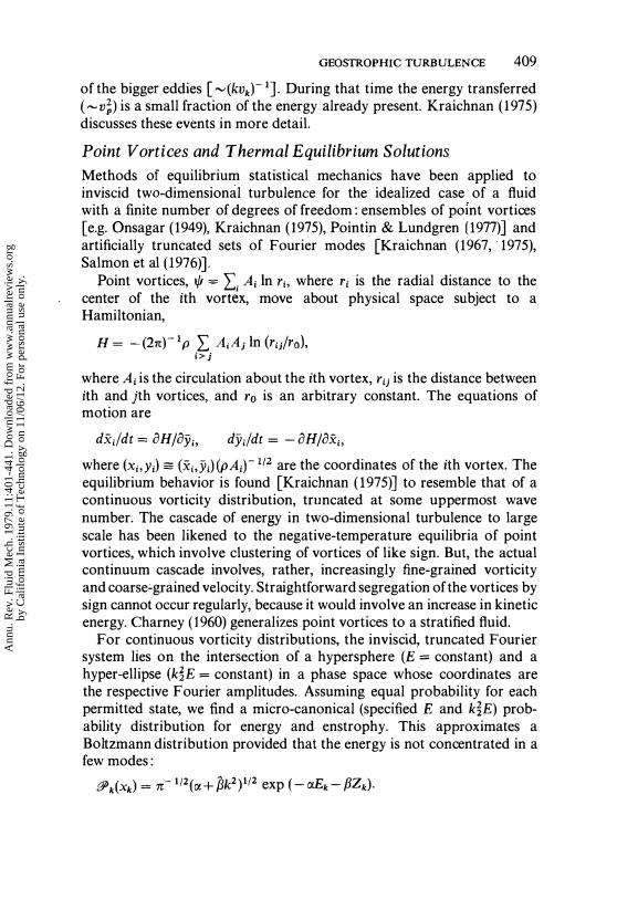
The simplest baroclinic cascade in this model, with initially small eddies (kip � 1), will act like two uncoupled layers of two-dimensional turbulence. The perspective of Figure 8 exhibits baroclinic motion on the upper plane, barotropic motion on the lower. Path c represents such a cascade, which (as in (J turbulence, path b) crosses into the wave regime as the wave steepness U//3L2 � 1.

Path d, however, reaches the stratification-controlled Rossby scale ft- 1/2 before encountering noticeably the {J effect. There, the fluid begins to communicate vertically: pressure perturbations build up as L increases with energy constant; cyclones above begin to uplift the interface, inducing cyclones below. This effect of vortex stretching is a familiar tendency in synoptic meteorology [e.g. Prandtl (1952), p. 386]. Here it acts forcefully, and path d jumps to the barotropic plane, proceeding once again as nearly depth-independent {J turbulence. Salmon et al (1976) show that the inviscid, truncated thermal equilibrium theory has a structure consistent with this evolution, strongly barotropic at large scale.

The change of vertical structure is a simple consequence of potential vorticity conservation (Rhines 1977). Take (J = 0, v � 0, and set t/12 = 0 at t = O. The lower layer evolves such that "V2t/12 + P(t/11 - t/12) = - Ft/1Y, following a fluid parcel (t/1Y is the initial value of t/1 I wherever the deep particle was at t = 0). Subject only to the unknown behavior of t/1?, the Fourier transforms (fJI and (fJ2 are related forever, (k2/P + 1)lh = lb 1 + lb?, where /ilY is the Fourier transform of the initial t/11 field distorted as if it were a passive tracer by the t/12 field. The ratio of potential to kinetic energy, P(k)/K(k) follows: P(k)/K(k) = y-1[1-215/(1 +152)J where y =

k2/2P, � = (1 + t/JYNl)f(1 +y). If the initial eddies were small, relative to the Rossby radius, ft-1/2,

soon t/J2 will far exceed t/JY, and the above relation shows that any energy reaching k = pI/2 has /il2//il1 = i. Energy reaching larger scales is ever more barotropic. At larger k, the interface rigidity causes /il2 � /ill. This is the only way in which the lower layer, with vanishing Q2, can allow flow to occur. The energy ratio, P / K, peaks at a value 0.2 near k = -/iF and falls to zero like k-2 above, and k2 below; with t/J? � t/J1> P/K �

y- I { 1- 2(1 + y)j[l + (1 + y)2J} (Figure 9). If, instead, the initial (/J? field had involved larger eddies, these results

would not seem to follow: except that we can then appeal to the enstrophy cascade to remove, eventually, t/J? == q� from finite scales. Thus, the q� field has contours that will be continually extended by the 1/12 turbulence,

Ann

u. R

ev. F

luid

Mec

h. 1

979.

11:4

01-4

41. D

ownl

oade

d fr

om w

ww

.ann

ualr

evie

ws.

org

by C

alif

orni

a In

stitu

te o

f T

echn

olog

y on

11/

06/1

2. F

or p

erso

nal u

se o

nly.

422 RHINES

and to the extent that this occurs, the above asymptotic results again obtain. (They tend not to obtain at wave numbers containing little energy. Particularly at large k, the rightward cascading field of Iii? is significant enough to exceed IiiI itself.) With the initial wave number kO � FI/2, the large eddies are heavy with potential energy, PIR' '" (k�F)-l. Yet after the cascade, the largest value of PI K in the field is 0.2, while much of the flow is barotropic. This amounts to a generalized baroclinic instability, followed by growth of barotropy. The details of e(k) == P + K are unknown, but eventually, minimizing enstrophy requires that the energy continually move toward k = 0, in a nearly perfect state of barotropy, PI K --io 0.

The association of declining potential ens trophy with conversion of potential to kinetic energy may be seen by writing q2 = P K + 2(F + k2)P. With C) = J(f ( ) dk,

q21e = [k�+2(p+knpIK]!(1+PIK),

where k� = k2 P, k1 = k2 K. Fixing kp and kK' q2 is monotonically increas­ing with PI K.

The initial evolution of these large baroclinic eddies is also visible in the conservation laws for total energy and q2 :

Er = 0,

1.0

0.5

0.5 1.0

Figure 9 The ratio of lower-layer to upper-layer stream-function amplitude, as a function of wave number, for two-layer stratified turbulence (p turbulence), after the ens trophy cascade has occurred. Also, the ratio of potential to kinetic energy. This plot closely describes the problem with small initial eddies, and approximately describes the energy­containing region of the general problem.

Ann

u. R

ev. F

luid

Mec

h. 1

979.

11:4

01-4

41. D

ownl

oade

d fr

om w

ww

.ann

ualr

evie

ws.

org

by C

alif

orni

a In

stitu

te o

f T

echn

olog

y on

11/

06/1

2. F

or p

erso

nal u

se o

nly.

�

CI".26 CIII.27 CI".47 CI .... 72

'¥z

CI= .077 Clo: .11 CI = .33 CI= .68

1=0 t= 1.5mo t� 2.5 t� 5.2 Figure lOa Free evolution of initially large-scale eddies (relative to the Rossby scale, P- 112). Here, the initial condition is a single baroclinic Rossby wave, plus noise. This is path e of Figure 8. The initial behavior is a linearized instability (an eddy-mean field interaction), yet mutual eddy in teractions quickly take over. The end-state has lost most of its potential energy, evolving into a zonally elongated pattern of energetic, fast-moving barotropic Rossby waves. Time, in months, 2000 km by 2000 km re-entrant ocean. CI means contour interval.

@ � "0 ::c .... ("l � '" 1:1' C � Q

i!3 w

Ann

u. R

ev. F

luid

Mec

h. 1

979.

11:4

01-4

41. D

ownl

oade

d fr

om w

ww

.ann

ualr

evie

ws.

org

by C

alif

orni

a In

stitu

te o

f T

echn

olog

y on

11/

06/1

2. F

or p

erso

nal u

se o

nly.

o � 2000 11m ie> �

"l', ,t���iPj�;�:'�)iiJ� � m X �

CI '.10

d 7]

o -�i ' I, " YJI/J/IJ/JJ//I/I;, ,:/, / !Ii!!; �

12.6 ..... ..� " ) """".J I, S-C\= .07

Figure lOb Time-longitude plot of the shallow and deep stream function, '1', and '1'2' and the temperature field, - fI, along a single latitude line, The evolution from depth-varying, baroclinic flow, to depth-dependent, barotropic flow causes the temperature eddies to vanish. Westward wave propagation coexists with the turbulent cascades. The propagation speed vastly accel erates after the mode tr ansition.

Ann

u. R

ev. F

luid

Mec

h. 1

979.

11:4

01-4

41. D

ownl

oade

d fr

om w

ww

.ann

ualr

evie

ws.

org

by C

alif

orni

a In

stitu

te o

f T

echn

olog

y on

11/

06/1

2. F

or p

erso

nal u

se o

nly.

GEOSTROPHIC TURBULENCE 425

The right-hand side of the ens trophy equation can act to increase the second moment of e if PI < O. If the initial field is large, k2 «i 2i, and then k2 Et "-' - 2 f P" so that this measure, k2 e, of the wave number content increases if P is converted to K.. This is how p turbulence temporarily avoids the "red" cascade of two-dimensional turbulence (which, never­theless, follows later on), and cascades toward k2 "-' i.

The cascade from large baroclinic eddies is shown as path e in Figure 8. In the presence of f3 it leads to a remarkable increase in both kinetic energy and wave-propagation speed as the field jumps from slow (baro­clinic) to fast (barotropic) modes. The streamline patterns from such a free cascade (Figure lOa) show the breakdown beginning as a baroclinic instability (i.e. eddy-mean flow interaction), but quickly turning into a chaotic state of eddy-eddy interaction. The lateral scale at first shrinks to � i- 1/2, then expands again as f3 turbulence. Meteorological numerical models (e.g. Simmons & Hoskins 1978, Williams 1978) suggest that the life cycles of midlatitude weather systems involve cyclic travel along path e. Weaker mean flows, which are only slightly unstable, fail to enter into the p turbulence cascade. Instead, they develop into a subtle inter­play of a few Fourier components (e.g. Pedlosky 1972). The time-longitude expression of path e (Figure lOb), shows an abrupt change in the wave propagation, as the turbulence alters both horizontal and vertical struc­ture. Again, waves coexist with a rapid turbulent cascade.

C losure Models

The development of a turbulence model that generalizes the notion of baroclinic instability as a cascade process has been initiated by Salmon ( 1978) and Blumen ( 1978). The eddy-damped Markovian model of Orszag (1970b, 1974) is adapted by Salmon incorporating both vertical and horizontal shear in the decorrelation time, J1. - 1, of the triple moments. The formulation is very like the diffusion approximation of Pouquet et al (1975) for two-dimensional turbulence.

For a statistically steady cascade driven by large-scale stirring, the spectra compare well with direct computer simulations (Figure 1 1). They show an overwhelming cascade toward barotropy (path e). Salmon (and the real atmosphere) demonstrate, however, that boundary friction can resist these inertial cascades, if the spin-down time is less than the int<rtial time scale, "-' U P1/2. Irregular horizontal boundaries can also defeat the cascade.

There are many observational and experimental studies that bear on p turbulence and yet retain their own distinctive nature ; for example, the rotating stratified "annulus" experiments (e.g. Hide 1953, Fultz 1959). Geostrophic turbulence, while it contains the universal aspect of stretching

Ann

u. R

ev. F

luid

Mec

h. 1

979.

11:4

01-4

41. D

ownl

oade

d fr

om w

ww

.ann

ualr

evie

ws.

org

by C

alif

orni

a In

stitu

te o

f T

echn

olog

y on

11/

06/1

2. F

or p

erso

nal u

se o

nly.

426 RHINES

2

o U 0\00

o o

o '0

\0 T >" v "' 2 \ o� \ O x. = 0 O�\

v ��

4 8 K

16

� \

32

Figure 11 Comparison of a closure model for steadily forced baroclinic instability (plus turbulent cascade), with numerical simulations (open circles) (Salmon 1978). u is the baro­tropic energy spectrum, :Y the baroclinic kinetic energy, with an adjustable parameter ..t. The tendency to barotropy is strong.

of q contours, must always be considered with the rather special forcing agents that create it.

An example from studies at Woods Hole Oceaonographic Institution (Schmitz 1978) shows currents at two sites in the North Atlantic. The first, Figure 12a, occurs in a region of modest (5 to 1 5 cm sec- l) current near 28°N, 700W (the MODE-73 experiment). It shows a waxing and waning of vertical coherence, as if nonlinear "capture" of one depth by another occurred, only to be defeated by friction or bottom topographic scattering. The second, Figure 12b, from near the Gulf Stream, represents the discovery of virtually barotropic currents in the deep ocean (see

-> Figure 12a Two short records from MODE-73 showing horizontal currents measured at two geographical stations (280 09'N, 680 39'W ; mooring 482) and (290 35'N, 700 W, mooring 489). The more quickly varying yet weaker currents in the deep water and brief episodes of great vertical coherence are commonplace. Each line is a horizontal current vector, plotted so that north is up.

Ann

u. R

ev. F

luid

Mec

h. 1

979.

11:4

01-4

41. D

ownl

oade

d fr

om w

ww

.ann

ualr

evie

ws.

org

by C

alif

orni

a In

stitu

te o

f T

echn

olog

y on

11/

06/1

2. F

or p

erso

nal u

se o

nly.

15 cm/s

15 cm/s

GEOSTROPHIC TURBULENCE 427

73 73 73 MAR APR MAY

7-:' 73 JUN JUL

03 '3 2'3 02 ,2 22 ci2 ,k 22 ci, ,\ 2' 0, ,', MAR APR MAY JUN JUL 73 73 73 73 7 3

4821 ( 406 M )

4823 ( 706 M )

4825 ( 1 411 M )

4826 ( 2936 M )

4827 ( 3957 M )

4828 ( 5128 M )

4891 ( 404 M )

4894 ( 1414 M )

4895 ( 2936 M )

Ann

u. R

ev. F

luid

Mec

h. 1

979.

11:4

01-4

41. D

ownl

oade

d fr

om w

ww

.ann

ualr

evie

ws.

org

by C

alif

orni

a In

stitu

te o

f T

echn

olog

y on

11/

06/1

2. F

or p

erso

nal u

se o

nly.

428 RHINES

u CD

•

J�� east

�--1 o c:

u> 40 E u

"0 0 Q) Q) Q. u>

r--T

600 m below surface

1 500m

4000 m

-40 May Sept Dec 75

Figure 12b Currents observed at a more energetic part of the North Atlantic, just south of the Gulf Stream (370 30'N, 550 Wi. Note different scales from Figure 12a. Here, the currents exhibit 50-day periods, roughly, and have penetrated right to the ocean bottom. Strong, depth-independent turbulence is characteristic of the analagous models. (See Schmitz 1978.)

Schmitz 1978}. This energetic site on the Sohm Abyssal Plain, has con­ditions ideal to encourage the enstrophy cascade to follow path e to its end.

5 TURBULENCE ABOVE TOPOGRAPHY Irregular bottom topography might seem an unpleasant detail to be appended onto the primary cascades represented in Figure 8. It affects the atmosphere, and particularly the ocean, however, at lowest order in

Ann

u. R

ev. F

luid

Mec

h. 1

979.

11:4

01-4

41. D

ownl

oade

d fr

om w

ww

.ann

ualr

evie

ws.

org

by C

alif

orni

a In

stitu

te o

f T

echn

olog

y on

11/

06/1

2. F

or p

erso

nal u

se o

nly.

GEOSTROPHIC TURBULENCE 429

the vorticity balance (e.g. Manabe & Terpstra 1974, Rhines 1969). In a homogeneous fluid, variations in depth h(x) and {3 each act through gradients in f /h to provide fixed fields of potential vorticity. Their respective length scales, however, are very different ; {3, the north-south gradient of Corio lis frequency, has the scale of the planetary radius, while h is distributed over a broad range, with one-dimensional spectrum typically proportional to k - 2 .

The relative strengths of topographic and inertial effects are measured not by c5 (the rins topographic height ...;- the mean depth across separations � L), but NRo, a much larger number for geostrophic flow. The scattering of linear topographic waves (wave-vector triads comprised of two Fourier components of flow and one of topography) sends energy and, more strongly, potential enstrophy, to small scale. The topography is a source of relative ens trophy, -i I V2t/1 1 2, which rises to such a level that inertial distortions are significant. This is opposite to the trend of f3 turbulence, and Figure 4, in which turbulence more usually evolved into waves.

The governing equation is Dq/Dt = 0, now with

q = V2t/1 + hi + {3y,

where hi = fo(h- H)/H, with H = h, the area-average mean depth, and hi / H � 1. We argued heuristically that the production of relative enstrophy, i ! V2t/1 ! 2, should be positive ; conservation of the area-average potential ens trophy, q2 then implies that mean correlation should develop between vorticity of the flow, and potential vorticity of the mean state,

a/at (hi + !3y) (V2t/1) = - a/at (V2t/1)2 < o. This correlation is the first sign of spontaneously growing time-average currents : anticyclones above seamounts, and broad westward flow in the interior of an enClosed basin (for which yV2t/1 < 0).

Under the right conditions, it is conceivable that topographic scatter­ing augments the cascade of q, but not so strongly that the kinetic energy itself is carried far toward large k. Bretherton & Haidvogel ( 1976) suggest that, then, the cascade is efficient enough to bring the fluid to a state of minimum potential ens trophy, invoking dissipation at the smallest scales. The time required to remove q2 from finite scales is just '" L/U.

Temporarily set f3 = 0 and let q2 = HS q2 dS, E = HI ! Vt/l ! 2 dS. The variational problem is to minimize q2 subject to fixed energy E. The boundary conditions are periodicity of t/I over a large distance L1 . We have

Oq2 + yoE = IV2(V2t/1 + hi - yt/l)ot/l dS = 0

Ann

u. R

ev. F

luid

Mec

h. 1

979.

11:4

01-4

41. D

ownl

oade

d fr

om w

ww

.ann

ualr

evie

ws.

org

by C

alif

orni

a In

stitu

te o

f T

echn

olog

y on

11/

06/1

2. F

or p

erso

nal u

se o

nly.

430 RHINES

for all infinitesimal variations, �1jJ, and y is a Lagrange multiplier. The solution requires V21jJ + h' = yljJ or

rJi = h/(y + k2), k2 = l k I2, where � and h are Fourier transforms. This is a unique, steady solution of the nonlinear equations. The energy level and topographic spectrum determine y. At scales small compared with y- l/2, q = V21jJ + h' � 0 ; fluid is carried over small'-scale bumps with relative vorticity responding to bottom-slope induced vortex stretching. At large scales (� y- l/2), IjJ � y - 1h ; the flow lies directly along geostrophic (depth) contours. IjJ is thus a low-pass filtered image of the topographic field (Figure 13).

With {3 reinstated, the analogous problem for an enclosed basin gives simply

11 (3 ljJ(x,y) = L k2 +- eik ' x + - y, k Y Y

plus a term representing inertial boundary layers at the walls. The effect is to add a large-scale westward flow [of the form discovered by F of on off ( 1954)J, whose strength {3IY depends on the initial energy level and topo­graphy. The production of a planetary-scale mean circulation is a remarkable consequence of the enstrophy cascade, acting on initially small-scale eddies. The minimum-ens trophy state can only be approxi­mate : an initial spatial distribution of energy that is far removed from this state cannot propagate in space quickly enough to establish it within the decay period for transients (the inertial time scale) ; the development of true steadiness is controversial ; only topographic spectra of "inter­mediate" slope (say ",k- 2) can be expected to allow enstrophy (but not energy) to cascade, and the relevance to a stratified fluid is uncertain.

( b)

(0)

Figure 13 The end-state of turbulence over rough bottom topography (Bretherton & Haidvogel 1976) : (a) the topography ; (b) the final stream function. The initial state for the free decay was a random pattern of eddies uncorrelated with the topography.

Ann

u. R

ev. F

luid

Mec

h. 1

979.

11:4

01-4

41. D

ownl

oade

d fr

om w

ww

.ann

ualr

evie

ws.

org

by C

alif

orni

a In

stitu

te o

f T

echn

olog

y on

11/

06/1

2. F

or p

erso

nal u

se o

nly.

GEOSTROPHIC TURBULENCE 431

Statistical turbulence models of Holloway (1976, 1978), Salmon, Holloway & Hendershott ( 1976) and Herring (1977) have been applied to "H turbulence," and promise a more complete picture of both the initial adjustment and the end-state.

Salmon et al (1976) give the inviscid equipartition spectrum for H turbulence. The Boltzmann distribution, as in Section 3, applies when there is a rich mix of modes :

el' i(Xi) = n- 1/2(0(+ I1kr) 1/2 exp [ - (0( + I1kt ) (Xi-<X;) 2], where <x;) = I1ki(O( + l1kl)- lQi ; Qi being the ith Fourier coefficient of the topographic plus beta effects, h'(x,y) + py. The energy spectrum at equilibrium is

<xl) = i(O(+ 13kf)- l + 112kt(0( + 13M)Ql

or just the sum of the two-dimensional turbulence equipartition spectrum and the energy of the steady geostrophic contour current, <Xi>. This maximum entropy solution has as its ensemble average the minimum potential enstrophy solution.

Holloway (1976, 1978) and Herring (1977) derive closure models for free-decay and steadily forced H turbulence, respectively. Holloway uses a modified test-field model, with a prescription for the decorre1ation time, (J, of the triple moments, which is approximately

(3(Jkpq)- 2 � vk(k)+ f: Z(p) dp + k- 2 f: p2Q(p) dp

- J: ( 1- p2P)R(P) dp for k <: kO. R is the covariance spectrum of vorticity and topography. The first term is linear viscosity ; the second is the strain rate at wave number k due to larger eddies ; the third is the decorrelative effect of topographic Rossby waves [of frequency '"V k - 1(Jp2Q dp)1/2] , and the final term represents the reduction in wavelike restoring forces when flow lies near the geostrophic (Q - constant) contours. A comparison of the turbulence model with numerical simulations, Figure 14, is encourag­ing. For a moderately strong initial eddy field, (/h' '"V 0.8, a significant time-averaged contour flow is found, superimposed on an enduring time-dependent eddy field. In the absence of viscosity the system relaxes to the absolute equilibrium described above.

The energy-transfer spectra in experiments (Rhines 1977) suggest that advective transfer toward small k (as in two-dimensional turbulence) can rise to balance the topographic scattering to large k, leaving a net spec­trum that evolves only very slowly.

Ann

u. R

ev. F

luid

Mec

h. 1

979.

11:4

01-4

41. D

ownl

oade

d fr

om w

ww

.ann

ualr

evie

ws.

org

by C

alif

orni

a In

stitu

te o

f T

echn

olog

y on

11/

06/1

2. F

or p

erso

nal u

se o

nly.

1 01r-e-

1 0°

1 0-1

1 0-2

1 0 1

K

Ll

1 02 10° 1 0 1

K

1 02

Figure 14 Comparison of closure theory and numerical simulations for H turbulence (Holloway 1 978). Here, the topographic spectrum, H, is k2/(1 +k4). Z is the vorticity spectrum, R the covariance spectrum between topography and vorticity, and Z the predicted static mean circulation. This is a free-decay problem, observed several inertial times after it began.

oj:::. VJ N

� :I: Z m C/O

Ann

u. R

ev. F

luid

Mec

h. 1

979.

11:4

01-4

41. D

ownl

oade

d fr

om w

ww

.ann

ualr

evie

ws.

org

by C

alif

orni

a In

stitu

te o

f T

echn

olog

y on

11/

06/1

2. F

or p

erso

nal u

se o

nly.

GEOSTROPHIC TURBULENCE 433 Herring (1977) has studied the complementary problem of H turbulence

driven by stationary random forcing. New topographic-dynamic inertial ranges are predicted. Rather simple forms are given for the transfer spectrum and relaxation time, which accord with the scale analysis of topographic and turbulent strain rates. Increasing the topographic height field has the effect of increasing the static contour flow, increasing the topographic wave frequencies, and decreasing the spectral energy trans­fer. The topographic parameter, biRo, determines the ratio of turbulent energy to static-flow energy.

These several approaches concur over the importance of (and form of) the steady-flow mode, as an outcome of a turbulent cascade. It is remark­able to have such explicit predictions of mean-flow generation by turbulence. Yet another view is given in Section 6, below.

Perhaps the weakest aspect of the turbulence models is their insistence on spatial homogeneity. Neither advection nor wave propagation is capable of smoothing the energy of the atmosphere and ocean, which has specific, sparse source regions. Heterogeneity of the bounding oro­graphy further aggravates the problem.

When density stratification is added back into the H turbulence problem, the cascade toward a barotropic vertical structure is severely altered. In fact, the baroc1inic structure observed to persist in ocean eddies (Figure 12a) may be largely due to bottom topography and severe spatial inhomogeneity (Owens & Bretherton 1977, Rhines 1977).

The H turbulence problem appropriate to the atmosphere is made rather different from these "oceanic" theories by a strong zonal flow, imposed at the outset. Manabe & Terpstra (1974), for example, show that mountains of modest proportions alter the energy transformations of the dominant baroc1inic eddies. The advected baroc1inic instabilities of a smooth-surfaced planet give way to orographically locked components.

6 MEAN-FLOW INDUCTION The transport of potential vorticity, if it takes any systematic form, can drive a mean circulation. The geostrophic-contour following flows of Section 5 are examples. For a local view, form the ensemble average of the quasi-geostrophic vorticity equation,

OOT < q) + (u> . V( q> = - V · ( q'u'> + <F) (6. 1 )

where u and V are horizontal and q = ( q) + q'. Without the eddy con­tribution, this equation describes the response to forcing (minus dissipa­tion), F, in the form of Rossby waves, Sverdrup circulation, or circulations with intrinsically nonlinear mean flow.

Ann

u. R

ev. F

luid

Mec

h. 1

979.

11:4

01-4

41. D

ownl

oade

d fr

om w

ww

.ann

ualr

evie

ws.

org

by C

alif

orni

a In

stitu

te o

f T

echn

olog

y on

11/

06/1

2. F

or p

erso

nal u

se o

nly.

434 RHINES

The eddy driving term, V ' (q'u'), can be rewritten in terms of the Lagrangian diffusivity of the fluid, acting on the mean large-scale field iJQ/iJx;, with important effects of forcing and dissipation (e.g. Rhines 1978). The Eulerian mean motions that result are the consequence of lateral Reynolds stresses and the vertical transmission of horizontal stress, by a combination of mean Coriolis torque and in viscid wave-drag exerted across deformed isopycnal surfaces.

Let us examine, first, a simple case in which lateral stresses are exerted by geostrophic eddies. Consider a polar p plane, with constant depth, density, and Corio lis frequency, f, decreasing linearly away from the center. Neglecting forcing and dissipation, we have simple conservation of barotropic potential vorticity,

q == py + (,

Dq = O. Dt

(6.2)

Here y,v are the (inward) radial coordinate and velocity. Integrate over a region within a fixed latitude circle, '6'. The Eulerian, zonally averaged u velocity is then given by

iJ 0 -7Ji!le = qv = - oy uv,

where (-) = J (!)( ) dx is the integral about the latitude circle. Now a fluid column that would have zero relative vorticity at latitude Yo has potential vorticity q = PYo == py - p(y - yo). With v = Dy/Dt, v = 0, and defining '1 = y - Yo, it follows that

OUe = - f3(y - ) D(y - Yo) ot

Yo Dt

where K22 is the north-south component of turbulent diffusivity. If the convective part of the right side is small, the above equation becomes

(6.3)

for an initial state of rest. The neglect of the convective terms leading to Equation (6.3) is not so severe as to require linear wave motion. It implies

Ann

u. R

ev. F

luid

Mec

h. 1

979.

11:4

01-4

41. D

ownl

oade

d fr

om w

ww

.ann

ualr

evie

ws.

org

by C

alif

orni

a In

stitu

te o

f T

echn

olog

y on

11/

06/1

2. F

or p

erso

nal u

se o

nly.

GEOSTROPHIC TURBULENCE 435

where y is a correlation coefficient between v and 1]2, U is a scale-particle speed, c a scale-phase speed, and L a length scale defining the north-south envelope of variation of 1]2. Equation (6.3) is thus valid for either weak disturbances (U / c � 1 ) or nonlinear fields in which the scale of variation L of the intensity is much greater than the typical north-south particle displacement.

Random trading of fluid particles across the latitude circle <{i sys­tematically decreases the net relative vorticity within Cfj, yielding an Eulerian mean circulation. This westward momentum appears at "free" latitudes for which Equation (6.2) holds. At forced latitudes, where the wave maker is located, eastward momentum is left behind as a prograde jet whose strength depends upon the nature of the wavemaker : net angular momentum vanishes if the source provides none. In the steadily excited inviscid case the westward circulation at a given latitude builds

up to its asymptotic value --!f3YJ2 as soon as the disturbance arrives. The eastward jet continues to accelerate indefinitely, to compensate for the presence of westward flow in an ever larger region. The central result, which holds in more general circumstances, is that the depth-averaged flux of potential vorticity equals the force, plus the momentum influx, exerted along <{i by eddies on the fluid instantaneously occupying the fixed contour, <{i. The association of momentum flux gradient with vorticity flux, and hence with turbulent transport of the (conservative) potential vorticity, was first made by Taylor ( 1 9 1 5). Kuo (e.g. 1 953), Bretherton ( 1966), Dickinson ( 1969), Green ( 1970), and Rhines ( 1977) have applied the idea to the atmospheric geometries ; it appears that turbulent vorticity transport accounts in part for the maintenance of the mean atmospheric zonal circulation, although nonrandom (monsoon­and orography-related) "eddies" are also important (e.g. Oort & Peixoto 1974).

Experiments demonstrating zonal flows emerging from random forcing on a sphere or f3-plane have been performed by Whitehead (1975), de Verdiere ( 1977), and Williams (1978). One experiment, Figure 5, from Williams's terrestrial simulations shows a clear, large-scale pattern of equatorial easterlies and mid latitude westerlies. de Verdiere (1977, Figure 15) has studied the rectified flows in the laboratory, driven by an articulated pattern of fluid sources and sinks.

As a final example, we illustrate the mean-motion patterns found in a model of an enclosed ocean basin driven by steady winds [Holland ( 1 978) ; see also Robinson et al ( 1977) and Semptner & Mintz ( 1977)] . Here, a

Ann

u. R

ev. F

luid

Mec

h. 1

979.

11:4

01-4

41. D

ownl

oade

d fr

om w

ww

.ann

ualr

evie

ws.

org

by C

alif

orni

a In

stitu

te o

f T

echn

olog

y on

11/

06/1

2. F

or p

erso

nal u

se o

nly.

(a) (b) Figure 15a The generation of zonal mean circulation on a laboratory "polar p-plane" (a rotating cylinder of water with a paraboloidal free surface) (de Verdiere 1977). Westward propagating waves are driven by fluid sources and sinks at the periphery ; at higher latitudes (nearer the cent�r) a "westward" circulation is driven by the eddies. Figure 15 b As in Figure 15a, but after halting the forcing of the eddies. The mean circulation remains behind.

..,. W 0\

� ::t: Z ttl ""

Ann

u. R

ev. F

luid

Mec

h. 1

979.

11:4

01-4

41. D

ownl

oade

d fr

om w

ww

.ann

ualr

evie

ws.

org

by C

alif

orni

a In

stitu

te o

f T

echn

olog

y on

11/

06/1

2. F

or p

erso

nal u

se o

nly.

GEOSTROPHIC TURBULENCE 437

new feature is the confinement by meridional boundaries, which block the geostrophic contours. The interior dynamics of Equation (6. 1) now resembles Sverdrup flow forced by eddies, rather than a much stronger zonal circulation found when the Q contours are "free."

In the deep water of Holland's model, there is a circulation driven entirely by eddies (Figure 16). The plotted particle trajectories illustrate both the strong eddy mixing and Lagrangian circulation. Whereas the lateral stresses described above are related to the flux of relative vorticity, <00, the mean motion here is driven by vertical stress trans-

geostrophic tu rbulence

southward boundary-f low

L/

Figure 16 Particle trajectories calculated from a numerical model of (Holland 1978). The domain is a 1000 by 2000 km basin, driven by steady winds (eastward at the central latitude, westward further north and south). This is the lower layer, which would have no motion, if it were not for the effect of the upper layer eddies. Both intense dispersion, and the systematic flow that it creates, may be seen. [Forty particles are released in clusters of four (from heavy dots).]

Ann

u. R

ev. F

luid

Mec

h. 1

979.

11:4

01-4

41. D

ownl

oade

d fr

om w

ww

.ann

ualr

evie

ws.

org

by C

alif

orni

a In

stitu

te o

f T

echn

olog

y on

11/

06/1

2. F

or p

erso

nal u

se o

nly.

438 RHINES

mission. This is fo\ufJ>IH, the flux of the isopycnal-Iayer thickness contribution to q (fJ is the height of the density interface between the two isopycnal layers). Since the flow is quasigeostrophic, U is proportional to the horizontal pressure gradient, andfo<urt>IH is related to the inviscid lateral pressure force JJpVrt dS exerted by the upper layer on the lower (e.g. Bretherton 1971, Rhines 1978).

This same inviscid wave drag is operating in the atmosphere. An example is the transmission of westerly stress downward to the ground in the strong mid latitude westerly jets (the depth-integrated eddy-mean flow interaction sees only the lateral Reynolds stresses). Another example is the stratospheric circulation driven by upward radiation of Rossby-gravity waves (e.g. Holton 1975). Although the perturbations are no longer turbulent, the form of the stresses is the same.

7 CONCLUSION The action of geostrophic turbulence, in cascading potential vorticity, q, upward through wave number space, largely determines the develop­ment of the energy-containing eddies. It is ironical that increasing the disorder in this way may lead to large-scale flow patterns, vastly unequal partition between potential and (favored) kinetic energy and between baroclinic and (favored) barotropic modes, conversion from turbulence into wave-motion, and from turbulence to a static component of large­scale circulation. It is the turbulent transport of q across physical space (in the presence of mean fields of q) that generates time- or ensemble­averaged flow, both eddy-scale circulations about bottom topographic features and planetary-scale drifts.

The spatial and spectral q-transports are useful diagnostics for numerical experiments and, when measurable, for observations of nature. The Lagrangian strain rates, seen in the dispersal of marked fluid elements, are a more visible sign of an intense turbulent cascade. The actual rate of disappearance of q from finite length-scales is of great interest, empirically ; much of the nature of the mean circulation depends upon the memory of the fluid's initial potential vorticity.

Energy dissipation is imagined to be a process far slower than q­dissipation in these models. Some geophysical examples, however, involve very thick boundary layers that prevent this large-Reynolds-number picture from occurring. Cyclones in the atmosphere, for instance, dissipate their kinetic energy in essentially the inertial time scale. The energy dissipation rate for the ocean is unknown ; it hinges on interaction with three-dimensional processes in the fluid interior, rather than boundary turbulence.

Ann

u. R

ev. F

luid

Mec

h. 1

979.

11:4

01-4

41. D

ownl

oade

d fr

om w

ww

.ann

ualr

evie

ws.

org

by C

alif

orni

a In

stitu

te o

f T

echn

olog

y on

11/

06/1

2. F

or p

erso

nal u

se o

nly.

GEOSTROPHIC TURBULENCE 439

Of the effects that resist the enstrophy cascade, we have mentioned wave propagation (due to large-scale Q fields), yet omitted the important possibility that solitons may develop. These permanent-form, isolated solutions of the nonlinear beta-plane equations avoid the cascade by having q constant along streamlines. The various soliton forms [both "round" (Stern 1975, Flier! 1977), and zonally elongated (Larichev & Reznik 1977, Redekopp 1977)] are not far from the states observed in geophysical fluids. They lie near the linear-nonlinear transition, in some cases with the kind of anisotropy observed in the beta-plane experiments. The crucial question is whether many of the boundary-value problems appropriate to geophysical fluids evolve naturally in the direction of these solutions, or instead act out fully the enstrophy cascade.

ACKNOWLEDGMENT

This work was suggested by the National Science Foundation, grants OCE-760-0992 (the POLYMODE research program) and OCE 21674. This is contribution number 4 192 of the Woods Hole Oceanographic Institution, and number 1 10 of the POLYMODE project.

Literature Cited

Batchelor, G. K. 1953. Homogeneous Tur­bulence. Cambridge Univ. Press

Batchelor, G. K. 1969. Computation of the energy spectrum in homogeneous t wo­dimensional turbulence. Phys. Fluids 12 : 233-38

Batchelor, G. K., Townsend, A. 1959. Turbulent diffusion. In Surveys in MechaniCS, ed. G. K. Batchelor, R. M. Davies. Cambridge Univ. Press

Bretherton, F. P. 1 966. Critical-layer in­stability in baroc1inic flows. Q. J. R. Meteorol. Soc. 92 : 325-34

Bretherton, F. P. 1971. The general linear­ized theory of wave propagation. Lect. appl. math . . Am. Math. Soc. 1 3 : 61-102

Bretherton, F. P., Haidvogel, D. 1976. Two-dimensional turbulence above topo­graphy. J. Fluid Meeh. 78 : 129-54

Blumen, W. 1978. Uniform potential vor­ticity flow, Pts. I, II. J. Atmos. Sci. 35 : 774-89

Charney, J. 1960. Experiments in numerical hydrodynamics. Proc. Symp. Appl. Math. 15, pp. 289-309. Am. Math. Soc.

Charney, J. 1971. Geostrophic turbulence. J. Atmos. Sci. 28 : 1087-95

Cocke, W. J. 1969. Turbulent hydrodynamic line stretching : consequences of isotropy. Phys. Fluids 12 : 2488

de Verdiere, C. A. 1977. Laboratory experi-

ments with geostrophic turbulence. PhD thesis. MJ.T./W.H.OJ. Progr. Oceanogr.

Dickinson, R. 1969. Theory of planetary­wave zonal flow interaction. J. Atmos. Sci. 26 : 73-8 1

Dickinson, R. 1978. Rossby waves-long­period oscillations of oceans and atmos­pheres. Ann. Rev. Fluid. Mech. 10 : 159-95

Ertel, H. 1942. Ein neuer hydrodynamischer Wirbelsatz. Meteorol. Z. 59 : 277-81

Fjprtoft, R. 1953. On the changes in the spectral distribution of kinetic energy for two-dimensional nondivergent flow. Tellus 5 : 225-30

Flier!, G. 1978. Solitons in one- and two­layer fluids. Submitted for publication

Fofonoff, N. P. 1954. Steady flow in a frictionless homogeneous ocean. J. Mar. Res. 1 3 : 254-62

Freeland, H., Rhines, P., Rossby, T. 1975. Statistical observations of the trajectories of neutrally buoyant floats in the North Atlantic. J. Mar. Res. 33 : 383-404

Fultz, D. and collaborators, 1959. Studies ofthermal convection in a rotating cylinder with some implications for large-scale atmospheric motions. Meteorol. Monogr. Boston : Am. MeteoroL Soc.

.

Green, J. 1970. Transfer properties of the large-scale eddies and the general circula­tion. Q. J. R Meteorol. Soc. 96: 1 57-85

Ann

u. R

ev. F

luid

Mec

h. 1

979.

11:4

01-4

41. D

ownl

oade

d fr

om w

ww

.ann

ualr

evie

ws.

org

by C

alif

orni

a In

stitu

te o

f T

echn

olog

y on

11/

06/1

2. F

or p

erso

nal u

se o

nly.

440 RHINES

Grimshaw, R. 1975. A note on the {:I-plane approximation. Tellus 27 : 351-57

Herring, 1. 1977. On the statistical theory of two-dimensional topogra�hic turbul­ence. J. Atmas. Sci. 32 : 2254-71

Herring, J., Orszag, S., Kraichnan, R., Fox, D. 1974. Decay of two-dimensional homogeneous turbulence. J. Fluid Mech. 66 : 41 7-44

Hide, R. 1953. Some experiments on thermal convection in a rotating liquid. Q. J. R. Metearal. Soc. 7 9 : 161-83

Holloway, G., Hendershott, M. 1977. Stochastic closure for nonlinear Rossby waves. J. Fluid Mech. 76: 617-721

Holland, W. 1978. The role of mesoscale eddies in the general circulation. J. Phys. Oceanagr. 8: 363-92

Holloway, G. 1976. Statistical hydro­mechanics : applications in mesoscale ocean circulation. PhD thesis. Univ. Calif., San Diego

Holloway, G. 1978. A spectral theory of nonlinear barotropic motion above ir­regular topography. J. Phys. Oceanagr. 8 : 414-27

Holton, J. 1975. A semi-spectral numerical model for wave mean-flow interactions in the stratosphere. J. Atmas. S d. 33 : 1 639-49

Hoskins, 8., Bretherton, F. 1972. Atmos­pheric frontogenesis models : mathemati­cal formulations and solutions. J. Atmas. Sci. 29: 1 1-37

Ibbetson, A., Tritton, D. 1975. Decay of turbulence in a rotating fluid. J. Fluid Mech. 67 : 444-49

Kraichnan, R. 1967. Inertial ranges in two­dimensional turbulence. Phys. Fluids 10 : 1417-23

.

Kraichnan, R. 1 97 1 . An almost Markovian, Galilean invariant turbulent model. J. Fluid Mech. 33 : 5 1 3-14

'Kraichnan, R. 1975. Statistical dynamics of two-dimensional flow. J. Fluid Mech. 67 : 155-75

Kuo, H. 1953. On the production of mean zonal currents in the atmosphere by large disturbances. T ellus 5 : 344-62

Larichev, V., Reznik, S. 1977. Solitary Rossby waves. Prac. Yalta Symp. in Mesoscale Ocean Dyn., Acad. Sci. USSR

Leith, C 1968. Diffusion approximation for two-dimensional turbulence. Phys. Fluids 1 1 : 671-72

Leith, C, Kraichnan, R. 1972. Predictability of turbulent flows. J. Atmas. Sci. 29: 1041-58

Lilly, D. K. 1969. Numerical simulation of two-dimensional turbulence. Phys. Fluids Suppl. 2 : 240-49

Lilly, D. K. 1971. Developing and decaying two-dimensional turbulence. J. Fluid

Mech. 45 : 395-415 Lilly, D. K. 1972. Numerical simulation

studies of two-dimensional turbulen ce : I. Models o f statistically steady turbul­ence. Geaphys. Fluid Dyn. 3 : 289-3 19

Manabe, S. , Terpstra, T. 1974. The effects of mountains on the general circulation of the atmosphere as identified in numeri­cal experiments. J. Atmas. Sci. 3 1 : 3-42

Merilees, P., Warn, H. 1975 . On energy and ens trophy exchanges in two-dimensional non-divergent flow. J. Fluid Mech. 69 : 625-30

Miles, J. 1974. On Laplace's tidal equation. J. Fluid Mech. 66: 241-60

Moffatt, H. 1967. On the suppression of turbulence by a uniform magnetic field. J. Fluid Mech. 2 8 : 571-92

Oort, A., Peixoto, J. 1974. The annual cycle of the energetics of the atmosphere in the planetary scale. J. Geaphys. Res. 79 : 2705-19

Onsager, L. 1949. Statistical hydrodynamics. Nuava Cimenta Supp. 6: 279-87

Orszag, S. A. 1970a. Comments on "Tur­bulent hydrodynamic line stretching : consequences of isotropy." Phys. Fluids 1 3 : 2203-04

Orszag, S. 1970b. Analytical theories of tur­bulence. J. Fluid Mech. 41 : 363-85

Orszag, S. 1974. Statistical Theory of Tur­bulence : Les Hauches Summer School on Physics. London : Gordon & Breach

Owens, W. B. Bretherton, F. P. 1977. A numerical study of mid-ocean mesoscale eddies. Deep-Sea Res. In press

Pedlosky, J. 1972. Limit cycles and un­stable baroclinic waves. J. Atmas. Sci. 29 : 53-63

Phillips, N. A. 1963. Geostrophic motion. Rev. Geaphys. 1 : 123-76

Pointin, Y., Lundgren, T. 1977. Statistical mechanics of two-dimensional vortices in a bounded container. Phys. Fluids 1 9 : 1459-70

Pouquet, A., Lesieur, M., Andre, J., Basdevant, C 1975. Evolution of high Reynolds number two-dimensional tur­bulence. J. Fluid Mech. 72 : 305-25

Prandtl, L. 1952. Essentials offiuid dynamics. New York : Hafner

Redekopp, L. 1977. On the theory of solitary Rossby waves. J. Fluid Mech. 82 : 725-45

Rhines, P. 1969. Slow oscillations in an ocean of varying depth, I, II. J. Fluid AJech. 37 : 161-205

Rhines, P. 1975. Waves and turbulence on a p-piane. J. Fluid Mech. 69 : 417-43

Rhines, P. 1977. The dynamics of unsteady currents. In The Sea, 6: 189-318. New York : Wiley

Rhines, P. 1978. Eddy-driven circulation of the ocean : a vorticity transport theory.

Ann

u. R

ev. F

luid

Mec

h. 1

979.

11:4

01-4

41. D

ownl

oade

d fr

om w

ww

.ann

ualr

evie

ws.

org

by C

alif

orni

a In

stitu

te o

f T

echn

olog

y on

11/

06/1

2. F

or p

erso

nal u

se o

nly.

J. Mar. Res. Submitted for publication Richardson, L. F. 1922. Weather predictions

by numerical process. Cambridge Univ. Press

Robinson, A., Harrison, D., Mintz, Y., Semptner, W. 1977. Eddies and the general circulation of an idealized oceanic gyre. J. Phys. Oceanogr. 7 : 182-207

Rossby, T., Voorhis, A., Webb, D. 1975. A quasi-Lagrangian study of mid-ocean variability using long-range SOFAR fioats. J. Mar. Res. 33 : 355-82

Salmon, R. 1978. Two-layer quasi-geostropic turbulence in a simple special case. Geophys. Astrophys. Fluid Dyn. 10: 25-53

Salmon, R., Holloway, G., Hendershott, M. 1976. The equilibrium statistical mech­anics of simple quasi-geostropic models. J. Fluid Mech. 75 : 691-703

Schmitz, W. 1978. Observations of the vertical distribution of kinetic energy in the western North Atlantic. J. Mar. Res. 36 : 295-3 10

Semptner, W., Mintz, Y. 1977. Numerical simulation of the Gulf Stream and mid­ocean eddies. J. Phys. Oceanogr. 7 : 208-30

GEOSTROPHIC TURBULENCE 441

Simmons, A., Hoskins, B. 1978. The Jife­cycles of some non-linear baroclinic waves. J. Atmos. Sci. 35 : 417-32

Starr, V. P. 1953. Note concerning the nature of the large-scale eddies in the atmosphere. T ellus 25 : 233-46

Stern, M. E. 1975. Nonlinear stationary, p-plane eddies. J. Mar. Res. 3 3 : 1-23

Taylor, G. I. 19 15. Eddy-motion in the atmosphere. Phi/os. Trans. R. Soc. London Ser. A 240 : 1-26

Taylor, G. 1. 1917. Observations and specu­lations on the nature of turbulent motion. In Scientific Papers, ed. G. K. Batchelor. Cambridge Univ. Press

Weinstock, J. 1 978. On the theory of turbul­ence in the buoyancy subrange of stably stratified flows. J. Atmos. Sci. 35 : 634-49

Whitehead, J. 1975. Mean flow driven by circulation on a p-plane. Tellus 27 : 358-64

Williams, G. P. 1975. Jupiter's atmospheric circulation. Nature 257 : 778

WiJliams, G. P. 1978. Planetary circulations : I, Barotropic representation of Jovian and terrestrial turbulence. J. Atmos. Sci. 35 : 1399-426

Ann

u. R

ev. F

luid

Mec

h. 1

979.

11:4

01-4

41. D

ownl

oade

d fr

om w

ww

.ann

ualr

evie

ws.

org

by C

alif

orni

a In

stitu

te o

f T

echn

olog

y on

11/

06/1

2. F

or p

erso

nal u

se o

nly.