Geostatistical modelling of uncertainty in soil science modelling of uncertainty in ......

Ž .Geoderma 103 2001 3–26www.elsevier.comrlocatergeoderma

Geostatistical modelling of uncertainty insoil science

P. Goovaerts)

Department of CiÕil and EnÕironmental Engineering, The UniÕersity of Michigan,EWRE Building, Room 117, Ann Arbor, MI 48109-2125, USA

Received 12 December 1999; received in revised form 22 June 2000; accepted 9 February 2001

Abstract

This paper addresses the issue of modelling the uncertainty about the value of continuous soilŽ .attributes, at any particular unsampled location local uncertainty as well as jointly over several

Ž .locations multiple-point or spatial uncertainty . Two approaches are presented: kriging-based andŽ .simulation-based techniques that can be implemented within a parametric e.g. multi-Gaussian or

Ž .non-parametric indicator frameworks. As expected in theory and illustrated by case studies, thetwo approaches yield similar models of local uncertainty, yet the simulation-based approach has

Ž .several advantages over kriging: 1 it provides a model of spatial uncertainty, e.g. the probabilityŽ .that a given threshold is exceeded jointly at several locations can be readily computed, 2

Ž .conditional cumulative distribution function ccdf for supports larger than the measurementŽ .support e.g. remediation units or flow simulator cells can be numerically approximated by the

cumulative distribution of block simulated values that are obtained by averaging values simulatedŽ .within the block, and 3 the set of realizations allows one to study the propagation of uncertainty

through global GIS operations or complex transfer functions, such as flow simulators that considermany locations simultaneously rather than one at a time.

The other issue is the evaluation of the quality or AgoodnessB of uncertainty models. Two newŽcriteria exceedence probability plot and narrowness of probability intervals that include the true

.values are presented to assess the accuracy and precision of local uncertainty models usingcross-validation. According to the second criterion, multi-Gaussian kriging performs better than

Ž .indicator kriging for the hydraulic conductivity HC data set. However, looking at the distributionŽ .of flow simulator responses, sequential indicator simulation sis yields better results than

Ž .sequential Gaussian simulation sGs that does not allow for significant correlation of extremeŽ .values destructuration effect . q 2001 Elsevier Science B.V. All rights reserved.

Keywords: Geostatistics; Uncertainty; Indicator kriging; Stochastic simulation; Accuracy

) Tel.: q1-734-936-0141; fax: q1-734-763-2275.Ž .E-mail address: [email protected] P. Goovaerts .

0016-7061r01r$ - see front matter q2001 Elsevier Science B.V. All rights reserved.Ž .PII: S0016-7061 01 00067-2

( )P. GooÕaertsrGeoderma 103 2001 3–264

1. Introduction

The last decade has witnessed an increasing awareness of the importance ofassessing the uncertainty about the value of soil properties at unsampledlocations, and of the need to incorporate this assessment in subsequentdecision-making processes, such as delineation of contaminated areas or identifi-cation of zones that are suitable for crop growth. Until the mid-1990s, uncer-tainty assessment has been essentially performed using non-linear kriging ap-

Ž .proaches e.g. disjunctive or indicator kriging that aim at evaluating theprobability for the target attribute to be no greater than any threshold value at a

Žspecific unmonitored location Webster and Oliver, 1989; Smith et al., 1993;.Goovaerts and Journel, 1995 . Nowadays, stochastic simulation algorithms are

becoming more common—or maybe just more AfashionableB—for uncertaintyŽmodelling in soil science Vanderborght et al., 1997; Pachepsky and Acock,

.1998; McKenna, 1998; Bloom and Kentwell, 1999; Broos et al., 1999 . TheŽ .basic idea is to generate a set of equiprobable representations realizations of

the spatial distribution of soil attribute values and to use differences amongsimulated maps as a measure of uncertainty. Again, there is a vast toolbox ofalgorithms available: sequential indicator or Gaussian simulation, turning bandmethod, p-field simulation, simulated annealing, to name a few.

Several authors have attempted to compare the performance of the manyflavors of non-linear kriging and stochastic simulation algorithms. To myknowledge, the most complete comparison of non-linear kriging algorithms has

Ž .been conducted by Papritz and Dubois 1999 . They found that all the non-linearmethods modelled the local conditional distributions of probability equally welland no method was consistently superior to others. Comparison of stochastic

Žsimulation algorithms has received more attention in the literature Deutsch,.1994; Gotway and Rutherford, 1994; Srivastava, 1996; Goovaerts, 1999a , but

the conclusion is essentially the same: there is no simulation algorithm that isbest for all cases, but rather a toolbox of alternative algorithms from which to

Žchoose or to build the algorithm best suited for the problem at hand Gomez-´.Hernandez, 1997a . Although most of the aforementioned papers have been´

published in congress proceedings that are not readily accessible to soil scien-tists, the aim of this paper is not to compare or even review the differentgeostatistical algorithms available for uncertainty modelling. Readers should

Ž .refer to recent books on the subject, such as Goovaerts 1997 , Deutsch andŽ . Ž .Journel 1998 or Chiles and Delfiner 1999 . The focus is here on the first-order`

decision of whether a kriging-based or a simulation-based approach should beadopted.

The choice of an approach for uncertainty modelling should be guided by theanswer to the questions discussed below.

Ž .1 What type of uncertainty model is being sought? In some applications, theŽobjective is to estimate the uncertainty prevailing at a particular location local

( )P. GooÕaertsrGeoderma 103 2001 3–26 5

.uncertainty , while other problems like flow modelling requires the uncertaintyabout soil attribute values to be assessed at many locations simultaneouslyŽ .multiple-point or spatial uncertainty .

Ž .2 What is the support for the uncertainty assessment? Decision-making isŽ .frequently performed over supports remediation units or agricultural fields that

are much larger than the measurement supports, hence some aggregation orup-scaling must be conducted.

Ž .3 Why do we model uncertainty? Assessing uncertainty about soil attributevalues is rarely a goal per se, rather it is often a preliminary step to evaluate therisk involved in any decision-making process or to investigate how predictionerrors propagate through complex functions, such as crop models, cost curvesfor wrong remediation decision or flow simulators.

Each issue will be reviewed in this paper and illustrated using two casestudies, see Fig. 1. The first data set, kindly provided by M.J.-P. Dubois of theSwiss Federal Institute of Technology, consists of 259 topsoil Cd concentrations

2 Ž .Fig. 1. Two data sets: 259 topsoil Cd concentrations measured in a 14.5-km area unitssmgrkg ,Ž .and 50 hydraulic conductivity HC data originating from the scanning of a block of sandstone.

The dashed box depicts a 0.25-km2 remediation unit for cadmium and flow simulator cell for HC.


2 Žmeasured in a 14.5-km area in the Swiss Jura Atteia et al., 1994; Webster et.al., 1994 . The objective is to assess the uncertainty about Cd concentration at

unsampled locations and to assess its impact on remediation decisions. TheŽ .second data are interpreted as 50 hydraulic conductivity HC data measured in a

cross-section of a soil profile. This data set is not synthetic, but results from theŽ .scanning of a block of sandstone Srinivasan and Journel, 1998 and the 50

values have been randomly drawn from the 102=102 original image; referencetrue values will be used to assess the quality of predictions. Because the initial

Ž .measurements porosity values have been rescaled, the units are meaninglessand are not included in this paper. The objective here is to assess the uncertaintyabout HC values at unsampled locations and its impact on the prediction of flowor solute transport.

Once the choice of a kriging-based or a simulation-based approach has beenmatured, there remains the problem of picking the algorithm that would yieldthe AbestB model of uncertainty. Since there is no AbestB algorithm for allsituations, different algorithms should be applied to the data and their respectiveperformances should be compared. Such a sensitivity analysis is frequentlyimplemented for spatial interpolation: kriging estimates are compared with

Žobservations that have been either temporarily removed one at a time leave-. Ž .one-out or cross-validation or set aside for the whole analysis jacKnife , and

statistics such as mean square or mean absolute errors of prediction areŽ .computed e.g. see Davis, 1987; Wackernagel, 1998, p. 91 . Assessing the

goodness of uncertainty models has received far less attention. For example,Ž .Goovaerts and Journel 1995 compared the performances of various indicator

kriging algorithms for predicting probabilities of deficiencies at test locationsŽ .jacKnife approach by computing the ratio of probabilities at locations that areactually sufficient or deficient: the larger the ratio the better the discriminationbetween the two types of location. More sophisticated measures of the goodness

Ž .of local uncertainty models have been recently proposed by Deutsch 1997 orŽ .Papritz and Dubois 1999 . These measures are briefly reviewed in this paper,Žand two new criteria exceedence probability plot and narrowness of probability

.intervals that include the true values are proposed to assess the accuracy andprecision of uncertainty models.

2. Modelling the local or the spatial uncertainty?

2.1. Local uncertainty

Consider the simplest situation where the uncertainty prevailing at a singlelocation u is to be modelled. The probabilistic way to model the uncertainty

Ž .about a continuous attribute z at u consists of: 1 viewing the unknown value


Ž . Ž . Ž .z u as the realization of a random variable Z u , and 2 deriving the condi-Ž . Ž .tional cumulative distribution function ccdf of Z u :

F u; zN n sProb Z u FzN n , 1� 4Ž . Ž . Ž . Ž .Ž .

Ž .where the notation A N n B expresses conditioning to the local information, say,Ž .n neighboring data z u The ccdf fully models the uncertainty at u since ita

gives the probability that the unknown is no greater than any given threshold z.ŽCcdfs can be modelled using either parametric a model is assumed for theŽ .multi-variate distribution of the random function Z u , commonly the multi-

. Ž . ŽGaussian distribution is adopted or non-parametric indicator approaches e.g..see Goovaerts, 1997, Chap. 7 . Their most salient features are discussed below.

Ø Under the multiGaussian model, the ccdf at any location u is Gaussian andfully characterized by its mean and variance, which correspond to the simplekriging estimate and variance at u. The approach typically requires a priornormal score transform of data to ensure that at least the univariate distributionŽ .histogram is normal. The normal score ccdf then undergoes a back-transformto yield the ccdf of the original variable.

Ø The indicator approach also begins with a non-linear transform of the data.In this case, each observation is transformed into a set of K indicator values

Ž .corresponding to K threshold values e.g. 9 deciles of the sample histogram . Kccdf values at u are estimated by a kriging of these indicator data, and thecomplete function is obtained by interpolationrextrapolation of the estimated

Ž .probabilities, see Goovaerts 1999b for more details on implementation of theindicator approach.

Both approaches are used to derive the ccdf of HC values at two locations u1Ž . Ž .small open circle and u large open circle depicted at the top of Fig. 2. For2

multi-Gaussian kriging, the mean and the variance of the ccdf in the normalŽ .space top graph was identified with the simple kriging estimate and variance,

Ž .then the horizontal axis was rescaled middle graph through a normal scoreback-transform. Bottom graphs show the model fitted to the nine ccdf valuesestimated at u and u using ordinary indicator kriging.1 2

Comparison of ccdfs in Fig. 2 shows that both parametric and non-parametricŽ .approaches yield similar models at u small circle . The steep ccdf indicates1

that the unknown HC value is more likely smaller than 1000, and the proximityto observations explains the smaller uncertainty prevailing at u relatively to u .1 2

Differences between uncertainty models are more pronounced at u . The spread2

of the parametric ccdf is mainly controlled by the kriging variance, which islarger than at u because of the greater distance to neighboring observations.1

The large spread of the non-parametric ccdf is caused by the wide range ofsurrounding HC values, which leads to a bimodal probability distribution with ahigh probability to be either below 250 or above 1500. Note that the relativegoodness of the parametric and non-parametric ccdfs can be assessed and


compared only if the actual HC value at u is known, and this issue will be2

discussed later in Section 5.

2.2. Spatial uncertainty

The two ccdfs of Fig. 2 provide information on the probability of any giventhreshold to be exceeded at u and u taken separately. For applications like the1 2

prediction of the time for fertilizers or contaminants to percolate across a soilprofile, it is critical to assess the probability that a series of locations are allabove a high threshold or are all below a small HC value: such strings of high orlow values may represent flow paths or barriers that control most of the flowand transport. For example, modelling the uncertainty prevailing jointly at u1

and u would require the inference of the two-point ccdf:2

F u , u ; z , z N n sProb Z u Fz , Z u Fz N n . 2� 4Ž . Ž . Ž . Ž . Ž .Ž .1 2 1 2 1 1 2 2

Ž .Inference of the joint probability 2 is straightforward if the two locations areŽ Ž ..uncorrelated: F u , u ; z , z N n is simply the product of the two one-point1 2 1 2Ž Ž .. Ž Ž ..probabilities F u ; z N n and F u ; z N n . This situation is however of1 1 2 2

little interest, and in presence of spatial correlation joint probabilities areŽestimated using either an analytical in most situations, a Gaussian model is

.adopted for the multivariate distribution of the random function or a numericalŽ .stochastic simulation approach.

Under the multi-Gaussian model, the two-point probability distribution isbivariate Gaussian and fully characterized by the mean and the variance of eachone-point ccdf, plus the covariance between u and u . Two shortcomings of the1 2

Ž .analytical approach are: 1 the spatial uncertainty assessment becomes veryŽ .complex as the number of grid nodes increases, and 2 it is cumbersome to

check in practice the validity of the bi-Gaussianity assumption, and data sparsityprevents us from performing such checks for more than two locations at a time.

The numerical approach consists of generating a set of L pairs of correlated� Ž l .Ž . Ž l .Ž .4values z u , z u , ls1, . . . , L, then estimating the joint probability1 2

from the set of simulated values as:

L1Žl . Ž l .F u , u ; z , z N n f i u ; z P i u ; z , 3Ž . Ž . Ž . Ž .Ž . Ý1 2 1 2 1 1 2 2L ls1

Žl .Ž .where the indicator value i u ; z is 1 if the simulated z-value at u does notj j j

exceed the threshold z , and 0 otherwise for js1,2. At least 100 simulationsjŽ .should be performed LG100 , which renders the approach computationally

Ž .Fig. 2. Location map of 50 HC data, and conditional cdf models provided by: 1 multi-GaussianŽ . Ž .kriging in the normal space top graph and after normal score back-transform middle graph , and

Ž . Ž .2 indicator kriging bottom graph at two grid nodes depicted by open circles.


more demanding than the analytical alternative. The procedure can however bereadily generalized to any number J of locations:

L J1Ž l .Prob Z u Fz , js1, . . . , JN n f i u ; z . 4Ž . Ž . Ž . Ž .� 4 ÝŁj j j jL js1ls1

Typically, the spatial distribution of soil attribute values is simulated over theentire domain of interest, then the joint probabilities can be computed for thetarget set of grid nodes. For example, Fig. 3 shows HC maps generated usingsequential simulation that proceeds as follows:

Ø Define a random path visiting only once each node to be simulated.Ø Model the ccdf at the first visited location uX conditional to the n original1

Ž .data z u .aŽ l .Ž X .Ø Draw from that ccdf a realization z u , which becomes a conditioning1

datum for all subsequent drawings....

X Ž X .Ø At the ith node u visited, model the conditional cdf of Z u given the ni iŽ . Ž l .Ž X .original data and all iy1 values z u simulated at the previouslyj

visited locations uX , js1, . . . , iy1.jŽl .Ž X .Ø Draw from the ccdf a realization z u , which becomes a conditioningj

datum for all subsequent drawings.Ø Repeat the two previous steps until all N nodes are visited and each has

been given a simulated value.

� Žl .Ž X . 4The resulting set of simulated values z u , js1, . . . , N represents onej� Ž . 4 Xrealization of the random function Z u , ugAA over the N nodes u . Anyj

� Žl .Ž X . 4number L of such realizations, z u , js1, . . . , N , ls1, . . . , L, can bej

obtained by repeating L times the entire sequential process with possiblydifferent paths to visit the N nodes.

Two major classes of sequential simulation algorithms can be distinguished,depending on whether the series of conditional cdfs are determined using the

Ž . Žmulti-Gaussian sGsssequential Gaussian simulation or the indicator siss.sequential indicator simulation formalism. Fig. 3 shows that the two algorithms

yield quite different results although the use of the same random path andsequence of random drawings for the paired sGs and sis realizations createssimilarities in the location of small and large simulated HC values.

The simulation procedure generates, at each location, a distribution of Lvalues which can be used to approximate numerically the ccdf. For example,

Ž . ŽFig. 4 top graph shows the cumulative distributions of 100 HC values black.dots simulated at u and u using sequential Gaussian simulation. The joint1 2

uncertainty prevailing at these two locations can be described by the scattergramŽ .of the 100 pairs of simulated values, see Fig. 4 left bottom graph . Because the

Ž .separation distance between u and u is larger than the range 24 units of the1 2


Ž .Fig. 3. Sets of three realizations generated using sequential Gaussian simulation sGs andŽ .sequential indicator simulation sis conditionally to the 50-HC data of Fig. 1.

normal score semivariogram model, the scattergram of simulated values displaysno correlation; hence, in this case, the joint probability distribution could beinferred directly from the two one-point distributions. This is not so if u is1

Ž .paired with the adjacent location u su q 1,0 , as illustrated by the correla-3 1Ž .tion of the corresponding simulated values Fig. 4, right bottom graph .


Ž .Fig. 4. Conditional cdf models inferred by multi-Gaussian kriging dashed line and numericallyŽ .through the generation of 100-HC values black dots using sequential Gaussian simulation at the

two grid nodes displayed in Fig. 2. The bottom graphs show the scattergrams of 100 pairs of HCŽ . Ž .values jointly simulated at two remote locations u , u or at two adjacent locations u , u .1 2 1 3

2.3. Stochastic simulation Õersus kriging

In several applications published so far in soil science, stochastic simulationhas been used merely to assess local uncertainty from the local distribution ofsimulated values; that is the ccdf at u is approximated by:

L1Ž l .F u; zN n f i u; z , 5Ž . Ž . Ž .Ž . Ý

L ls1

Ž l .Ž . Žl .Ž .where i u; z s1 if z u Fz, and 0 otherwise. In theory, as the number ofŽ .realizations tends to infinity L™` , the local distribution of simulated values

should match that provided by kriging within a similar framework. For example,the ccdfs inferred using multi-Gaussian kriging at u and u are overlaid over1 2

Ž .the cumulative distributions of 100 simulated HC values black dots in Fig. 4


Ž .top graph . Clearly, the kriging-based and simulation-based approaches yieldsimilar uncertainty models. Thus, if one seeks only a location-specific assess-

Ž .ment of uncertainty e.g. derivation of probability maps the use of stochasticsimulation entails an unnecessary waste of CPU time and disk storage.

3. Change of support

All the techniques presented in Section 2 allow one to model uncertainty overŽ .supports area or block similar to the observations’ one, which is usually small

if soil cores have not been bulked. In many situations, the uncertainty need to beŽ .assessed for much larger supports Heuvelink and Pebesma, 1999 , such as

remediation units for cadmium or flow simulator cells for hydraulic conductiv-ity, see Fig. 1. The objective is then to assess the probability that the averagez-value over a block of size V centered on u is no greater than any threshold z,that is to model the block ccdf:

F u; zN n sProb Z u FzN n . 6� 4Ž . Ž . Ž . Ž .Ž .V V

Under the multiGaussian model, ccdfs can be inferred using a proceduresimilar to the one described above, except that simple block kriging is now usedto derive the mean and variance of block ccdfs in the Gaussian space before the

Žback-transform of the horizontal axis e.g. see Chiles and Delfiner, 1999, p.`.445 . A limitation of the technique is that the attribute values must average

linearly in space which is, for instance, not the case for hydraulic conductivity.Also, the multi-Gaussian assumption may not be appropriate for the data understudy.

Limitations inherent in multiGaussian block kriging are not shared by theŽ . Žvolume–variance correction VVC approach Isaaks and Srivastava, 1989,

. Ž . Ž Ž ..Chap. 9 , which proceeds in two steps: 1 the point ccdf F u; zN n is firstŽ .inferred at the central location u of the block of size V, and 2 the point ccdf isŽ Ž ..corrected for the support effect to yield the block ccdf F u; zN n . SuchV

correction typically involves a decrease of the ccdf variance going from point toŽthe block support, while the shape of the ccdf remains the same permanence of

. Ž .distribution or becomes less skewed more symmetric with shorter tails . Theratio of the block and point ccdf variances, known as the variance reduction

Ž .factor f , is estimated from the z-semivariogram model as Journel, 1987 :

Var Z u N n g V , V� 4Ž . Ž . Ž .Vfs s1y F1, 7Ž .

Var Z u N n g AA, AA� 4Ž . Ž . Ž .

Ž . Ž .where g V, V and g AA, AA are the average semivariogram values within theblock V and the study area AA, respectively. If the area AA is large with regard to


Ž .the range of the semivariogram, the g AA, AA can be set equal to thesemivariogram sill, and f is estimated as:

fs1yg V , V , 8Ž . Ž .S

Ž . Žwhere g V, V is the average value of the standardized z-semivariogram unitS.sill within the block V and is approximated by the arithmetic average of the

standardized semivariogram values defined between any two discretizing pointsuX and uX within that block:i j

N N1X X

g V , V f g u yu .Ž . Ž .Ý ÝS S i j2N is1 js1

For a given reduction factor f , the block ccdf can be derived from the pointccdf using various algorithms that differ in the degree of symmetrizationimparted to that block ccdf. The affine correction amounts at keeping unchangedboth the mean and the shape of the point ccdf, regardless of the magnitude ofthe change of support. This permanence hypothesis is realistic only for smallblocks with little variability of z-values within them. Intuitively, one wouldexpect a gradual symmetrization of the block ccdf as the block size increases,which is achieved by the indirect lognormal correction implemented in Gslib

Ž .software, e.g. see Isaaks and Srivastava 1989, p. 473–475 for details.A more versatile—yet computationally intensive—alternative to the block

kriging and VVC approaches is provided by stochastic simulation. The blockccdf is numerically approximated by generating many simulated block values asŽ . Žnon linear averages of simulated point values Journel and Huijbregts, 1978, p.

.511 :L1

Ž l .F u; zN n f i u; z , 9Ž . Ž . Ž .Ž . ÝV VL ls1

Žl .Ž . Žl .Ž .where i u; z s1 if z u Fz, and 0 otherwise. For example, the simulatedV V

average Cd concentration within the 0.25-km2 block of Fig. 1 is computed asthe arithmetic average of the Js25 simulated point values falling into it:

J1XŽ l . Ž l .z u s z u . 10Ž . Ž . Ž .ÝV jJ js1

Ž .The attractive features of the simulation approach are that: 1 non-linearŽ . Ž .averaging functions e.g. geometric or harmonic mean can be considered, 2 no

assumption is made regarding the impact of the change of support on the shapeŽ .and variance of the block ccdf, and 3 once the grid of point values has been

simulated, ccdfs for various block sizes and shapes can be derived at littlecomputational cost.

Ž .Fig. 5 top left graph, solid line shows the cumulative distribution of 100simulated block values computed from the set of 100 sis Cd maps; the first three


Fig. 5. Block ccdfs modelling the uncertainty about the average Cd concentration over the0.25-km2 block delineated by the dashed line in Fig. 1. Three different approaches are used:multi-Gaussian block kriging, correction of an indicator-based point support ccdf model, and

Ždistribution of 100 block Cd concentrations simulated using sequential indicator simulation first.three realizations are displayed .

realizations with the corresponding block simulated values are also displayed inFig. 5. Such an uncertainty assessment is non-parametric: no prior assumption ismade about the shape of the distribution of possible values. For the same block,

Ž .the ccdf is also derived by multi-Gaussian block kriging dashed line andindirect lognormal correction of the ccdf inferred using indicator kriging at the

Ž .center of the block dotted line, fs0.24 . Although the three block ccdfs havesimilar median values, the upper and lower tails strongly differ. In particular, theVVC approach yields a much larger block variance with a higher probability ofoccurrence for both small and large average Cd concentrations.

4. How does the uncertainty propagate?

Our representations of the spatial distribution of soil attribute values arefrequently imported into functions of various complexity, such as economic


remediation models, crop models or flow simulators. The uncertainty about theinput soil attribute values will propagate through these AtransferB functions,

Ž .leading to uncertain response values such as non remediation costs, crop yieldsor flow travel times. Depending on the nature of the transfer function, variousapproaches can be used to assess the response uncertainty.

4.1. Local transfer functions

A transfer function is said to be local if it is applied to a single location u orŽ .block V u at a time. For example, the cost of classifying a location as safe with

Ž .respect to Cd could be modelled as a function of the concentration z u at thatparticular location:

0 if z u FzŽ . cy u s , 11Ž . Ž .½ z u yz otherwiseŽ . c

where z s0.8 mgrkg is the regulatory threshold for Cd. Similarly, the impactc

of soil acidity on the growth of a particular crop can be modelled as a functionŽ .of the local pH value z u :

°1 if z u F5Ž .~0 if z u )7Ž .y u s . 12Ž . Ž .¢7yz u r2 if 5-z u F7Ž . Ž .Ž .

The propagation of uncertainty from z- to y-values can be approached eitherŽ .analytically or numerically. Heuvelink 1998 provides a comprehensive review

of analytical propagation of local uncertainty. Because these methods rely onstringent assumptions on the distribution of input values, one may prefer a

Ž .numerical approach Monte-Carlo simulation , whereby the ccdf of z at u is� Ž l .Ž .randomly sampled many times, yielding a set of simulated z-values z u ,

4 Ž . Ž .ls1, . . . , L , which are then fed into functions of type 11 or 12 to generate a� Žl .Ž . 4set of simulated y-values y u , l, . . . , L . For example, the distribution of

Ž .possible health costs in Fig. 6 right bottom graph is obtained through a randomŽ .drawing of 1000 simulated Cd values and their post-processing by function 11 .

Random sampling of ccdfs can be very time-consuming, and a more efficientŽ .strategy is Latin hypercube sampling LHS that consists of dividing eachŽ .distribution into N equiprobable classes 100, for example , and sampling these

Žclasses without replacement to generate a set of N outcomes stratified random.sampling . In this way, the input distributions are represented in their entirety,

and it requires a much smaller sample than the Monte Carlo approach for aŽ .given degree of precision Mckay et al., 1979; Helton, 1997 . Recent application

Ž .of LHS in soil science can be found in Hansen et al. 1999 , Pebesma andŽ . Ž .Heuvelink 1999 , Van Merveinne and Goovaerts 2001 .


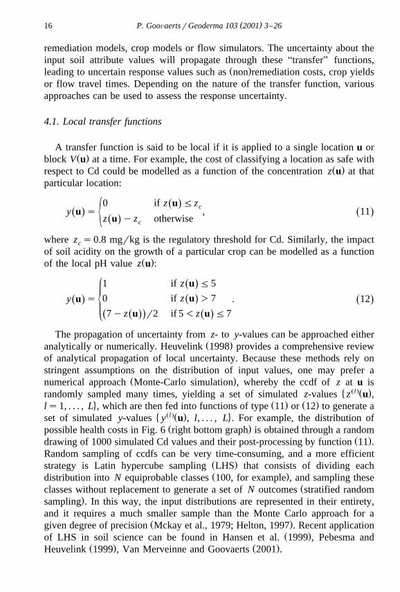
Ž .Fig. 6. Use of Monte-Carlo simulation random sampling of ccdf to propagate the uncertaintythrough local transfer functions. Application to the assessment of the uncertainty about healthcosts arising from the uncertainty about the Cd concentration at a particular location.

Uncertainty about the parameters of the transfer function itself can beaccounted for by sampling probability distributions of these parameters andcombining both simulated parameter and input z-values. For many parametersŽ .say more than five , the number of possible combinations becomes quicklyprohibitive, although an LHS strategy may greatly alleviate the computationalrequirements. When these parameters are correlated, their distributions cannotbe sampled independently and particular sampling techniques must be used, see

Ž .Viscarra Rossel et al. 2001 .

4.2. Global transfer functions

Complex transfer functions, such as flow simulators, truly propagate theuncertainty across the study area, which precludes the use of analytical proce-

Ž .dures in most situations—see Dettinger and Wilson 1981 for the use of thefirst order analysis as an alternative. The common approach is to generate manyrealizations of the spatial distribution of attribute values which are then fed into


the flow simulator to yield a distribution of response values, such as travel timesfor flow and solute transport. For example, Fig. 7 shows the histograms of water

Ž .travel times across the HC data set SW corner to NE corner obtained bypost-processing two sets of 100 sGs and sis realizations. These graphs confirmthe visual interpretation of Fig. 3 that the two sequential simulation algorithmsgenerate different sets of realizations, although they are all based on the same 50HC data. In particular, the response distribution is much narrower for sisrealizations.

The characterization of the space of uncertainty is rendered difficult by thefact that only a limited number of realizations is usually generated. A frequentand still open question relates to the number of realizations needed to samplefairly this space. For a given simulation algorithm and response variable, the

Žimpact of the number of realizations on the accuracy inclusion of the true. Ž .value and precision narrowness of the response distribution can be investi-

Ž .gated using the procedure described in Goovaerts 1999a .

4.3. Stochastic simulation Õersus kriging

Stochastic spatial simulation is usually not recommended for the local transferfunctions, since an LHS of ccdf provides similar results with much less CPUcosts. There are, however, two situations where a simulation-based approach iswarranted: transfer functions are available only for supports much larger than

Žthe measurement support e.g. remediation costs are known only for remediation.units of a given size , which requires a prior simulation-based derivation of the

Ž .block ccdf, and 2 the histogram of response values averaged over the studyarea is sought. Consider, for example, the problem of assessing the economicimpact of declaring the entire study area safe with respect to Cd. The distribu-

Fig. 7. Histograms of water travel times obtained by post-processing 100-sGs and 100-sis HCmaps through a flow simulator. The black dot in the box plot below each histogram is the truetravel time. Five vertical lines are the 0.025 quantile, lower quartile, median, upper quartile, and0.975 quantile of the distribution.


Ž .tion of global cost would be built by applying the cost function 11 to the set ofsimulated point values and averaging the local costs for each realization, see

Ž .Goovaerts 1999b, Fig. 7 .

5. How good is the model of uncertainty?

The previous sections have shown that different methods yield models ofuncertainty that can greatly differ, and a legitimate question is whether the

Ž .choice of a technique e.g. multi-Gaussian versus indicator kriging can besupported by the data. Like spatial interpolation, alternative techniques can beused to build uncertainty models which are then compared with observations

Ž .that have been either temporarily removed one at a time cross-validation or setŽ .aside for the whole analysis jacKnife . The remaining issue is the selection of

performance criteria for uncertainty assessment.

5.1. Local uncertainty

Ž Ž ..At any test location u, knowledge of the ccdf F u; zN n allows theŽ .computation of a series of symmetric p-probability intervals PI bounded by

Ž . Ž .the 1yp r2 and 1qp r2 quantiles of that ccdf. For example, the 0.5-PI isw y1Ž Ž .. y1Ž Ž ..xbounded by the lower and upper quartiles F u; 0.25N n , F u; 0.75N n .

A correct modelling of local uncertainty would entail that there is a 0.5probability that the actual z-value at u falls into that interval or, equivalently,that over the study area, 50% of the 0.5-PI include the true value. If a set ofz-measurements and independently derived ccdfs are available at N locations,

�w Ž . Ž Ž ..x 4u , z u , F u , zN n , js1, . . . , N , the fraction of true values falling intoj j j

the symmetric p-PI can be computed as:

N1j p s j u ; p ;pg 0,1 13Ž . Ž . Ž .Ý jN js1

with:

1 if Fy1 u ; 1yp r2 -z u FFy1 u ; 1qp r2Ž . Ž . Ž .Ž . Ž .j j jj u ; p s .Ž .j ½0 otherwise

The scattergram of the estimated versus expected fractions is called AaccuracyŽ .plotsB. Fig. 8 left top graph shows, for the HC data set, accuracy plot

computed for both parametric and non-parametric ccdfs using a cross validationŽ .of the 50 observations. Most of the points fall below the 458 line, i.e. j p -p

for most p, which reflects the inaccuracy of the probabilistic models. Forexample, the 0.5 probability intervals derived from the parametric approach only


ŽFig. 8. Plots of the proportion of true HC values falling within probability intervals accuracy.plot , and the width of these intervals versus the probability p. Top graphs relate to symmetric

intervals centered on the ccdf median, while bottom graphs depict results for unbounded intervals.Ž . Ž .Parametric multi-Gaussian and non-parametric indicator algorithms are used to derive ccdf

models in a cross-validation approach.

contain 40% of the true values. While the parametric models yield the largestdeviations between the estimated and theoretical fractions for small p-values,they perform better than the non-parametric models for large p-values. DeutschŽ .1997 proposed to assess the closeness of the estimated and theoretical fractionsusing the following AgoodnessB statistics:

1Gs1y 3a p y2 j p yp d p , 14Ž . Ž . Ž .H

0


Ž .where the indicator function a p is defined as:

1 if j p GpŽ .a p s .Ž . ½0 otherwise

Ž . ŽTwice more importance is given to deviations when j p -p inaccurate. < Ž . <case . The weight 3a p y2 s2 instead of 1 for the accurate case, that is the

case where the fraction of true values falling into the p-PI is larger thanexpected. For the cross validation of Fig. 8, the differences between the twoapproaches, as assessed by the goodness statistics G, are negligible: 0.902Ž . Ž .non-parametric and 0.899 parametric , which agrees with Papritz and Dubois’Ž .1999 conclusions.

Not only should the true value fall into the PI according to the expectedprobability p, but this interval should be as narrow as possible to reduce theuncertainty about that value. In other words, among two probabilistic modelswith similar goodness statistics, one would privilege the one with the smallest

Ž .spread less uncertain . Different measures of ccdf spread can be used: variance,interquartile range, entropy. In this paper, it is proposed to plot, for a series ofprobabilities p, the average width of the PIs that include the true values; see

Ž . Ž .Fig. 8 right top graph . For a probability p, the average width W p iscomputed as:

N1y1W p s j u ; p P F u ; 1qp r2Ž . Ž . Ž .Ž .Ý j j

Nj pŽ . js1

y1yF u ; 1yp r2 . 15Ž . Ž .Ž .j

Fig. 8 indicates that the parametric intervals are narrower until ps0.8,which may cause the proportion of true values falling into these intervals to besmaller than for the non-parametric models.

For applications where the exceedence of specific threshold values is themain concern, median-centered PIs could be replaced by unbounded PIs; for

w y1Ž Ž .. xexample, the 0.5-PI is now defined as F u; 0.5N n , q` or, in practice,w y1Ž Ž .. xF u; 0.5N n , z . A correct modelling of local uncertainty would entailmax

that over the study area, 50% of the true values locally exceed the ccdf median.Ž Ž ..Fractions Eq. 13 are thus computed as:

N1j p s j u ; p ;pg 0,1 16Ž . Ž . Ž .Ý jN js1

with:

1 if Fy1 u ; pX -z uŽ . Ž .j jj u ; p sŽ .j ½0 otherwise


where pXs1yp. Particular types of accuracy plots, called Aexceedence proba-bility plotsB, are created by plotting the estimated fractions versus the expected

Ž .ones; see Fig. 8 bottom left graph . Both parametric and non-parametric modelsyield similar fractions that are slightly larger than the expected ones for smallprobabilities p corresponding to high HC values, pX-quantiles, while the propor-

Ž .tion of true values that exceed low HC thresholds high p values is smallerthan expected. The last graph shows the width of probability intervals which

Ž .corresponds here to the difference between the maximum z-value 2100 and thepX-quantile of the ccdf; for example, for ps0.1, the PI is bounded by the 9thdecile and the maximum value. As for symmetric PIs, multi-Gaussian krigingperforms better than indicator kriging in that the probability intervals are

Ž .narrower larger precision , while including similar proportions of true valuesŽ .similar goodness .

5.2. Spatial uncertainty

Unlike models of local uncertainty that can be compared to actual observa-tions, there is no reference spatial distribution of values to use as yardstick formodels of spatial uncertainty. Classical checks, which amount at verifying thequality of the reproduction of histogram and semivariogram by the realizations,provide no indication on the goodness of the set of realizations as a whole. Insome instances, information might be available on the actual response value fora particular transfer function. For example, field tests may allow an accurateprediction of the travel time of contaminants or flow between two locations.This field observation can then be compared with the distribution of timesderived by post-processing a set of HC realizations through a flow stimulator. Inthis particular case, one may also adopt geostatistical inverse methods that allowthe use of the output variable to calibrate the geostatistical model in a cokriging

Ž .environment Zhang and Yeh, 1997 or actually condition simulated realizationsŽ .Gomez-Hernandez et al., 1997b .´ ´

In this paper, the true travel time has been computed from the reference102=102 image and is depicted by a black dot on the histograms of Fig. 7. Forthe HC data set, sequential indicator simulation clearly yields the best results

Ž .since the response distribution is narrower greater precision , while includingŽ . Žthe true value accuracy . Thus, it appears that the greater precision narrower

.PI of the parametric ccdfs does not entail a greater precision of the model ofresponse uncertainty because flow simulation is influenced primarily by thespatial distribution of HC values.

6. Conclusions

Uncertainty assessment, which should become a key step of any geostatisticalanalysis of soil data, can take various forms, such as mapping the probability of


exceeding threshold values or generating sets of realizations of the spatialdistribution of attribute values. As for spatial prediction, the users are faced withthe difficult choice of an algorithm within the geostatistical toolbox, and the aimof this paper was to review briefly the tools available to address various issues,such as the modelling of uncertainty over supports of different sizes or thepropagation of uncertainty through local or global transfer functions.

The primary question is whether stochastic simulation is required for uncer-tainty assessment, or whether similar information can be acquired by thecomputationally cheaper kriging approach. There are two situations where there

Ž .is no good alternative to stochastic simulation: 1 propagation of uncertaintyŽ .through multiple-point dynamic transfer functions, such as flow simulators,

Ž .and 2 the modelling of uncertainty over supports much larger than theŽ .measurement supports for attributes like hydraulic conductivity that do not

average linearly in space. In all other situations—which may represent themajority of current applications of geostatistics to soil science—a kriging-basedmodelling of ccdf and its subsequent Latin-hypercube sampling for numericalpropagation of uncertainty should be the first choice.

For both stochastic simulation and kriging-based approaches, the commonŽ . Ž .issue is whether a parametric multi-Gaussian or non-parametric indicator

approach should be adopted. There is no straight answer to that question, and forccdf modelling it is recommended to perform a cross-validation to assess thegoodness and precision of models of local uncertainty. For example, accuracyplots can be computed using a Gslib-type program available on http:rrwww.ualberta.car;cdeutschr. For spatial uncertainty and its propagation throughcomplex transfer functions, there is usually no way to assess the quality ofmodels. Users should then keep in mind that the multi-Gaussian model does notallow for any significant spatial correlation of very large or very small valuesŽ . Ž .destructuration effect , which may not be desirable conservative for theapplication of interest. In the case of the HC data set, a parametric approach wasbetter for modelling local uncertainty, while for propagation of spatial uncer-tainty, best results were obtained using a non-parametric algorithm.

In this paper, the focus has been on the modelling of uncertainty for singlecontinuous soil attributes. Many soil attributes are categorical and uncertaintyassessment through indicator-based kriging or stochastic simulation has receivedan increasing attention the last few years, e.g. see Bierkens and BurroughŽ . Ž . Ž .1993a,b , Goovaerts 1996 , Oberthur et al. 1999 . Again, the issue of assess-¨ing the goodness of such models has rarely been addressed and criteria similar tothe ones introduced here could be developed. In several situations, there is also aneed for modelling the joint uncertainty about the values of multiple soilattributes at a single location or across the entire domain. Similarly, transferfunctions, such as crop models, frequently include many input variables whichrequires a multivariate propagation of uncertainty. In the future, more researchshould be devoted to issues such as the multivariate modelling of ccdfs or the


spatial cosimulation of variables, and the joint sampling of multiple ccdfs usingLHS.

References

Atteia, O., Dubois, J.-P., Webster, R., 1994. Geostatistical analysis of soil contamination in theSwiss Jura. Environ. Pollut. 86, 315–327.

Bierkens, M.F.P., Burrough, P.A., 1993a. The indicator approach to categorical soil data: I.Theory. J. Soil Sci. 44, 361–368.

Bierkens, M.F.P., Burrough, P.A., 1993b. The indicator approach to categorical soil data: II.Application to mapping and land use suitability analysis. J. Soil Sci. 44, 369–381.

Bloom, L., Kentwell, D.J., 1999. A geostatistical analysis of cropped and uncropped soil from theJimperding Brook catchment of Western Australia. In: Gomez-Hernandez, J., Soares, A.,´ ´

Ž .Froidevaux, R. Eds. , geoENV II—Geostatistics for Environmental Applications. KluwerAcademic Publishing, Dordrecht, pp. 369–379.

Broos, M.J., Aarts, L., van Tooren, C.F., Stein, A., 1999. Quantification of the effects of spatiallyvarying environmental contaminants into a cost model for soil remediation. J. Environ.Manage. 56, 133–145.

Chiles, J.-P., Delfiner, P., 1999. Geostatistics: Modelling Spatial Uncertainty. Wiley, New York.`Davis, B.M., 1987. Uses and abuses of cross validation in geostatistics. Math. Geol. 19, 241–248.Dettinger, M.D., Wilson, J.L., 1981. First order analysis of uncertainty in numerical models of

groundwater flow: Part I. Mathematical development. Water Resour. Res. 17, 149–161.Deutsch, C.V., 1994. Algorithmically-defined random function models. In: Dimitrakopoulos, R.

Ž .Ed. , Geostatistics for the Next Century. Kluwer Academic Publishing, Dordrecht, pp.422–435.

Deutsch, C.V., 1997. Direct assessment of local accuracy and precision. In: Baafi, E.Y., Schofield,Ž .N.A. Eds. , Geostatistics Wollongong ’96. Kluwer Academic Publishing, Dordrecht, pp.

115–125.Deutsch, C.V., Journel, A.G., 1998. GSLIB: Geostatistical Software Library and User’s Guide.

2nd edn. Oxford Univ. Press, New York, 369 pp.Gomez-Hernandez, J.J., 1997a. Issues on environmental risk assessment. In: Baafi, E.Y., Schofield,´ ´

Ž .N.A. Eds. , Geostatistics Wollongong ’96. Kluwer Academic Publishing, Dordrecht, pp.15–26.

Gomez-Hernandez, J.J., Sahuquillo, A., Capilla, J.E., 1997b. Stochastic simulation of transmissiv-´ ´ity fields conditional to both transmissivity and piezometric data: I. Theory. J. Hydrol. 203,162–174.

Goovaerts, P., 1996. Stochastic simulation of categorical variables using a classification algorithmand simulated annealing. Math. Geol. 28, 909–921.

Goovaerts, P., 1997. Geostatistics for Natural Resources Evaluation. Oxford Univ. Press, NewYork, 512 pp.

Goovaerts, P., 1999a. Impact of the simulation algorithm, magnitude of ergodic fluctuations andnumber of realizations on the spaces of uncertainty of flow properties. Stochastic Environ. Res.Risk Assess. 13, 161–182.

Goovaerts, P., 1999b. Geostatistics in soil science: state-of-the-art and perspectives. Geoderma 89,1–45.

Goovaerts, P., Journel, A.G., 1995. Integrating soil map information in modelling the spatialvariation of continuous soil properties. Eur. J. Soil Sci. 46, 397–414.

Gotway, C.A., Rutherford, B.M., 1994. Stochastic simulation for imaging spatial uncertainty:


Ž .comparison and evaluation of available algorithms. In: Armstrong, M., Dowd, P.A. Eds. ,Geostatistical Simulations. Kluwer Academic Publishing, Dordrecht, pp. 1–21.

Hansen, S., Thorsen, M., Pebesma, E.J., Kleeschulte, S., Svendsen, H., 1999. Uncertainty insimulated nitrate leaching due to uncertainty in input data: a case study. Soil Use Manage. 15,167–175.

Helton, J.C., 1997. Uncertainty and sensitivity analysis in the presence of stochastic and subjectiveuncertainty. J. Stat. Comput. Simul. 57, 3–76.

Heuvelink, G.B.M., 1998. Error Propagation in Environmental Modelling with GIS. ResearchMonographs in GIS Series, London, 127 pp.

Heuvelink, G.B.M., Pebesma, E.J., 1999. Spatial aggregation and soil processes modelling.Geoderma 89, 47–65.

Isaaks, E.H., Srivastava, R.M., 1989. An Introduction to Applied Geostatistics. Oxford Univ.Press, New York, 561 pp.

Journel, A.G., 1987. Geostatistics for the Environmental Sciences. EPA project no CR 811893.Technical report, US Environmental Protection Agency, EMS Laboratory, Las Vegas, NV.

Journel, A.G., Huijbregts, C.J., 1978. Mining Geostatistics. Academic Press, New York, 600 pp.McKay, M.D., Beckman, R.J., Conover, W.J., 1979. A comparison of three methods for selecting

values of input variables in the analysis of output from a computer code. Technometrics 21,239–245.

McKenna, S.A., 1998. Geostatistical approach for managing uncertainty in environmental remedi-ation of contaminated soils: case study. Environ. Eng. Geosci. 4, 175–184.

Oberthur, T., Goovaerts, P., Dobermann, A., 1999. Mapping soil texture classes using field¨texturing, particle size distribution and local knowledge by both conventional and geostatisticalmethods. Eur. J. Soil Sci. 50, 457–479.

Pachepsky, Y., Acock, B., 1998. Stochastic imaging of soil parameters to assess variability anduncertainty of crop yield estimates. Geoderma 85, 213–229.

Ž .Papritz, A., Dubois, J.-P., 1999. Mapping heavy metals in soil by non- linear kriging: anŽ .empirical validation. In: Gomez-Hernandez, J., Soares, A., Froidevaux, R. Eds. , geoENV II´ ´

—Geostatistics for Environmental Applications. Kluwer Academic Publishing, Dordrecht, pp.429–440.

Pebesma, E.J., Heuvelink, G.B.M., 1999. Latin hypercube sampling of Gaussian random fields.Technometrics, in press.

Smith, J.L., Halvorson, J.J., Papendick, R.I., 1993. Using multiple-variable indicator kriging forevaluating soil quality. Soil Sci. Soc. Am. J. 57, 743–749.

Srinivasan, S., Journel, A.G., 1998. Direct simulation of permeability field conditioned to well testdata. In: Report 11, Stanford Center for Reservoir Forecasting, Stanford, CA.

Srivastava, M.R., 1996. An overview of stochastic spatial simulation. In: Mowrer, H.T.,Ž .Czapleweski, R.L., Hamre, R.H. Eds. , Spatial Accuracy Assessment in Natural Resources

and Environmental Sciences: Second International Symposium, General Technical ReportRM-GTR-277. US Department of Agriculture, Forest Service, Fort Collins, pp. 13–22.

Vanderborght, J., Jacques, D., Mallants, D., Tseng, P.H., Feyen, J., 1997. Analysis of soluteredistribution in heterogeneous soil: II. Numerical simulation of solute transport. In: Soares,

Ž .A., Gomez-Hernandez, J., Froidevaux, R. Eds. , geoENV I—Geostatistics for Environmental´ ´Applications. Kluwer Academic Publishing, Dordrecht, pp. 283–295.

Van Meirvenne, M., Goovaerts, P., 2001. Evaluating the probability of exceeding a site-specificsoil cadmium contamination threshold. Geoderma 102, 63–88.

Viscarra Rossel, R.A., Goovaerts, P., McBratney, A.B., 2001. Assessment of the production andeconomic risks of site-specific liming using geostatistical uncertainty modelling. Environ-

Ž .metrics 12 5 , in press.Wackernagel, H., 1998. Multivirate Geostatistics. 2nd edn. Springer, Berlin, 291 pp.


Webster, R., Oliver, M.A., 1989. Optimal interpolation and isarithmic mapping of soil properties:VI. Disjunctive kriging and mapping the conditional probability. J. Soil Sci. 40, 497–512.

Webster, R., Atteia, O., Dubois, J.-P., 1994. Coregionalization of trace metals in the soil in theSwiss Jura. Eur. J. Soil Sci. 45, 205–218.

Zhang, J., Yeh, T.-C.J., 1997. An iterative geostatistical inverse method for steady flow in thevadose zone. Water Resour. Res. 33, 63–71.

Geostatistical modelling of uncertainty in soil science modelling of uncertainty in ......

Documents

Transcript of Geostatistical modelling of uncertainty in soil science modelling of uncertainty in ......