Geophysical Surveys Near Tucson Electric Power

Sundt Generating Station

Geophysics Field Camp 2014 LASI-14-1

May 10, 2014

Lujain Ali Alghannam Wadyan Osama Ayyad

Carla Gabriela Do Lago Montenegro Wanjie Feng

Christopher A. Jones Mikhail D. Samoylov

Ben K. Sternberg Chak Hau Tso Sean T. Wright

1

Abstract

Tucson Electric Power (TEP) is carrying out subsurface investigations in order to locate more

groundwater for cooling at the Sundt power-generating plant. To assist with this investigation,

the University of Arizona GEN/GEOS 416/516 Field Studies in Geophysics class conducted

geophysics surveys in an area just south of Davis-Monthan Air Force Base and between UTM

coordinates 508,555 to 511,753 East and 3,553,705 to 3,556,895 North. Four geophysics

methods (Gravity, Magnetics, Transient Electromagnetics (TEM), and Passive Seismic) were

employed to locate a postulated fault, which may be correlated with ground water flow. A broad

regional magnetic anomaly was mapped, as the magnetic field decreases steadily from NE to

SW. There are no significant magnetic field anomalies that could be related to a potential fault.

The Gravity results show a regional gravitational gradient, steadily decreasing from NE to SW,

with a large isolated anomaly apparent around 1500m from the base station at the NE corner of

the survey area. But, this large anomaly is a localized, and does not appear on the adjacent

parallel survey lines, therefore it is not related to a potential fault contact. The Passive Seismic

survey detected a deep boundary at 100m to 160m in elevation, but the depths interpreted from

the 11 stations are scattered and do not show a clear trend. The Transient Electromagnetic (TEM)

data show a consistent difference in depth to a low-resistivity layer along the profile line. The

four TEM stations north of Interstate 10 (I10) have an average elevation for the 10 Ohm-m

contour line of 720 meters. The four TEM stations south of I10 have an average elevation for

the 10 Ohm-m contour line of 670 meters. This offset may be related to the postulated fault.

2

Acknowledgements

The University of Arizona Geophysics Field Camp class, GEN/GEOS 416/516, would

like to thank Tucson Electric Power for providing the funding for this project. In particular, we

would like to thank Byron Brandon of TEP for his coordination of the project. Without this

funding and support, we would not have been able to offer the class this year.

We would also like to thank the U.S. Geological Survey for their support of the class,

including identifying this project, and making the cooperation with Tucson Electric Power

possible. In particular, we would like to thank Don Pool for his coordination of the project. The

USGS also provided the passive seismic equipment.

Buck Schmidt, Principal Hydrologist of Basin Wells Associates, PLLC, presented the

geological background and objective of this project in an early class. His presentation and

assistance in this class were of great help to us in understanding the requirements of this project.

Jamie P. Macy, USGS Hydrologist, Arizona Water Science Center, Flagstaff Programs,

provided the TEM equipment and assisted us in the TEM field surveys. He taught us the

procedures for data acquisition and data processing. His willingness in sharing his expertise with

this class was invaluable for us.

We really appreciated the help from Don Pool. He arranged for our use of the Passive

Seismic equipment. He also taught us how to obtain the data and trained us on using the

processing software, Geopsy. He also double checked our processing results. His help let us be

confident in our processing results.

Zonge International provided data processing software to the class. Zonge International

has played a vital role in our Geophysics Field Camp for the past 27 years. We sincerely

appreciate that they have continued to provide our students with the opportunity to use state-of-

the-art electrical geophysics methods.

3

Table of Contents

Abstract

Acknowledgement

1. Introduction

1.1 History of site

1.2 Project Background and Outline

1.3 Reference

2. Location Maps

2.1 Geographic location

2.2 Gravity Survey Location

2.3 Magnetic Survey Location

2.4 TEM Survey Location

2.5 Passive Seismic Survey Location

2.6 Culture Interference

3. Magnetic Survey

3.1 Introduction

3.2 Dates and Location

3.3 Instruments and Field Procedures

3.4 Data Processing

3.5 Interpretation

3.6 Reference

4

4. Gravity Survey

4.1 Introduction, Instrumentation and Data Collection

4.2 Locations

4.3 Data Processing

4.4 Results

5. Passive-Seismic Survey

5.1 Introduction

5.2 Instrumentation and Field Procedures

5.3 Data and Results

5.4 Data Interpretation

5.5 Discussion and Conclusion

5.6 Reference

6. Transit Electromagnetic Survey

6.1 Introduction

6.2 Location

6.3 Instruments and Field Procedures

6.4 Data Processing

6.5 TEM Processing Results

6.6 Interpretation

6.7 Reference

Appendix A Magnetic Field Data

Appendix B TEM Data Fits and Models

5

1. Introduction

1.1 Tucson Basin Geology

Based on a deep exploration well commissioned by Exxon, Houser et al. (2004) describe

in detail the geologic settings of the Tucson Basin. This is among one of the best descriptions of

the Tucson Basin available, and is summarized in the following paragraphs. The Tucson Basin

was formed around the late Cenozoic, however Proterozoic and Paleozoic geologic events

shaped the area of the present Tucson Basin. The basin is located in the upper plate of the

Catalina detachment fault. Based on the deep exploration well logs, it was found that granitoid

rocks were penetrated beneath 3,658m of Mesozoic and Cenozoic sedimentary and volcanic

rocks. Uplift of the adjacent Catalina Mountains has altered the subsurface geometry of the

Basin. A stratigraphic section from Pleistocene to middle Miocene covers the top 1,880m of the

area. The Tucson Basin is a large structural basin, sediment filled and separated by mountain

ranges. It is 15 to 40km wide; 80km long, and the elevation is about 727m above sea level.

The top 1,880m of basin-fill sedimentary rocks can be divided about equally into the

lower basin-fill and upper basin-fill deposits. They consist of alluvial-fan, alluvial-plain, and

playa facies. The first 341m thick unit is an alluvial fan deposit that is a major aquifer in the

Tucson Basin. At about 908m there is a boundary that separates an unconsolidated and

undeformed upper-basin fill from a denser and more faulted lower-basin fill, indicating two

stages of basin filling. The Pontano Formation follows the sedimentary layers and it extends

deeper than the focus of this study.

1.2 Project Background and Outline

Tucson Electric Power (TEP) Sundt Power Plant has plans for expanding and improving

its well field to supply sufficient groundwater resources for power generation and cooling. An

aging well field along with declining groundwater levels has resulted in operational water supply

challenges with respect to groundwater yield and quality, and sand production. The improved

well field has to be able to provide at least 5500 gallons per minute (gpm) and the water must

have low temperature and total dissolved solids (TDS), since the water is used for cooling

purposes in the power plant. The TEP Sundt Groundwater Resource Investigation/Groundwater

6

Action Plan (GAP) is a project commissioned in order to find additional water resources in an

area close to TEP. The study area of the GAP is shown in Figure 1.1 (Bostic and Schmidt,

2013). A regional aquifer in a stratigraphic unit called the Upper Tinaja Beds (TSU) is the

optimal aquifer for meeting the requirements. This is because the yield potential of a shallower,

perched aquifer is too low and the existing deeper regional aquifer is expected to have

unacceptably high temperatures. Figure 1.2 shows the water depth of the regional aquifer in the

study area. Figure 1.3 shows a table with these stratigraphic units.

In order to assist with these goals, the GEN/GEOS 416-516 Field Studies in Geophysics

class performed four different geophysics surveys (Gravity, Magnetics, Transient

Electromagnetics (TEM), and Passive Seismic) in the area (Figures 1.1 and 1.2) where a

postulated fault crosses the regional and deep regional aquifers. The exact location of the fault is

unknown, as well as the exact depths of the aquifers. The proposed depth and location of the

fault is shown in Figures 1.4 and 1.5. The purpose of the geophysical studies and this report is to

provide additional information regarding the fault and the depths of the aquifers and aquitards,

and provide information for the proposed well locations. The following sections discuss each of

the geophysical surveys performed and the results obtained.

1.3 References

Bostic, Michael W., R.G Werner 'Buck' Schmidt, 2013, Tucson Electric Power - Sundt Generating Station, Preliminary Groundwater Resource Investigation, Tucson, Arizona, Prepared For Tucson Electric Power, September 4, 2013, Basinwells Associates Pllc Project No. 13-003

Houser, B., Peters, L., Esser, R., & Gettings, M. (2004, January 1). Stratigraphy and Tectonic History of the Tucson Basin, Pima County, Arizona, Based on the Exxon State (32)-1 Well. Stratigraphy and Tectonic History of the Tucson Basin, Pima County, Arizona, Based on the Exxon State (32)-1 Well. Retrieved April 20, 2014, from http://pubs.usgs.gov/sir/2004/5076/

Schmidt, Buck (February 3, 2014), TEP Sundt Groundwater Reource Investigation/Groundwater Action Plan (GAP), PowerPoint presentation, Power point presentation, BasinWells Associates, PLLC, Tucson AZ

7

Figure 1.1 GAP study area. The blue line represents the profile line of our survey area. The

yellow lines correspond with the cross sections shown in Figures 1.3 (A-A`) and 1.4 (B-B`),

courtesy of BasinWells Associates PLLC.

8

Figure 1.2 Depth to water of regional aquifer in the survey area.

9

Figure 1.3 Stratification, courtesy of BasinWells Associates PLLC.

Figure 1.4 Hydrogeologic cross section A-A`, courtesy of BasinWells Associates PLLC.

10

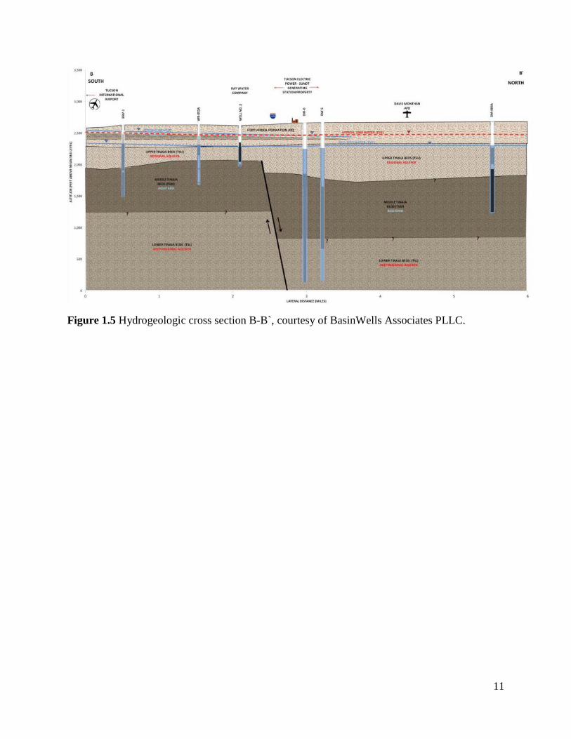
Figure 1.5 Hydrogeologic cross section B-B`, courtesy of BasinWells Associates PLLC.

11

2. Location maps

2.1 Geographic location

The survey area is located near the southern boundary of Tucson, just south of Davis-

Monthan Air Force Base, and with UTM coordinates 508,555 to 511,753 East and 3,553,705 to

3,556,895 North. The main profile is from the north-east corner of Section 11 to the south-west

corner of Section 15. Near the north-east corner of Section 11, a large solar array obstructs the

main profile line. Directly south of the solar array, two rail tracks cross the main profile. Further

southwest, Interstate 10 (I-10) bisects the main profile. A housing subdivision is located at the

south-west corner of the survey area. Four different geophysics methods (Gravity, Magnetics,

Passive Seismic and Transient Electromagnetics) were used in these surveys. The survey

locations for the four methods are shown in Figure 2.1.

2.2 Gravity Survey Location

A relative gravity meter was employed for the gravity survey. There are 38 Gravity

stations in total and 4 profiles. The direction of each profile is approximately NE-SW, 45 degree

NE. From a base station in the north-east corner to the last station in the south-west corner, the

overall length of the main profile line is 4335 m, with 11 stations. The gravity profile north-west

of the main transect is 700 m in length, with 8 stations. The central profile line straddles the main

profile and is 920 m long, with 8 stations. South-east of the main profile, another profile was

surveyed; it is 1000 m, comprised of 11 stations. The locations of these gravity stations and

profiles are shown in Figure 2.2.

2.3 Magnetic Survey Location

The magnetic survey was carried out along the main diagonal line of the survey area. A

total of 89 stations were measured. When encountering the solar array and subdivision, the

magnetic measurements were taken at least 20m away from the solar array fence and 50m away

from the subdivision to avoid interference from structures. The whole profile length is 4336m.

Figure 2.3 shows the locations of the 89 magnetic stations.

12

2.4 TEM Survey Location

It is necessary to use a large transmitting loop for a TEM survey. The size of each loop

used for this study was 200m X 200m. A total of eight loops were recorded, four on the north-

east side of I-10, and four on the south-west side of I-10. Due to the location of the solar array, I-

10, cacti, and the subdivision, the quantity and locations of these TEM loops were limited

(Figure 2.4).

2.5 Passive Seismic Survey Location

The passive seismic survey consists of eleven locations throughout the study area (Figure

2.5). These measurements were located primarily along the diagonal line of the survey area in

the northeast portion of the study area. Seismic measurements are more dispersed in the

southwest portion.

2.6 Culture interference

A number of structures limited our ability to follow a line orthogonal to the postulated

regional fault. Around the north east corner, there is a solar array. At the south-west side of the

solar array, a rail-track cuts through the main profile. High-voltage power lines and the I-10

bisect the main profile line. A subdivision is at the south-west corner of the survey area. The

main profile also encountered cacti and bushes.

13

Fig 2.1. Google Earth image of the survey area. Four geophysical methods applied along a Northeast-Southwest profile.

Passive Seismic

TEM

Gravity

Magnetic 1500 m

14

Figure 2.2 Gravity stations in the survey area; a total of 38. Two additional profiles, lateral from the primary Southwest-Northeast profile, were taken between I-10 and Rail track in order to locate the position of fault.

0 300 1500 m

15

Figure 2.3. Magnetic survey stations. The magnetic survey are mainly from the north-east corner to the south-west corner. There are 89 stations in total.

0 300 1500 m

16

Figure 2.4. TEM survey stations. The loop size for TEM survey is 200m × 200m. There are 8 loops in the survey area.

0 300 1500m

17

Figure 2.5. Passive Seismic survey stations. There are 11 stations in total.

0 300 1500 m

18

3. Magnetic Survey

3.1 Introduction

Magnetic surveys are one of the tools that exploration geophysicists use in order to map

oil, water, minerals, or other buried structures by measuring the Earth’s magnetic-field intensity.

The magnetic-field measurements respond to variations in the magnetic susceptibility of the

Earth materials. A large number of stations are needed to measure the magnetic field using

approximately constant distances between stations over the desired region and must be away

from metallic materials and roadways. In addition, a base station was set up to measure the

magnetic field simultaneously with the moving station. The base station is used to remove

temporal variations in the Earth’s magnetic field. A profile of the magnetic field can be

generated, which can illustrate the location of the anomalous body (U.S. Army Corps of

Engineers, 1995, 6-1).

3.2 Dates and Location

The magnetic field survey took place on February 8, 9, and 22, and April 6 of 2014. The

magnetic field data were collected in the south part of Tucson, along a diagonal line that crosses

Interstate 10 from northeast to southwest. A total of 89 stations were recorded along the profile

line, which encountered a solar array (northeast of I-10), and a subdivision (southwest of I-10)

that required shifts in the line. Measurements were not possible near the railroad and Interstate

10. Figure 3.1 shows the locations at which magnetic field measurements were taken.

3.3 Instrument and Field procedures.

The magnetometers used for this survey were the GEM Systems GSM-19 Overhauser

Magnetometer, the EDA OMNI IV Magnetometer, and the EDA OMNI Plus Magnetometer. We

used Garmin 530HX GPS receivers (Garmin International Inc. 2007) to determine the locations

of the stations. On the first weekend, a base station was set up at the beginning of the line at the

southwest corner between Craycroft road and Drexel road. We started to take measurements

every 50m along the main profile. During that first weekend (Feb 7th-8th) measurements around

the solar array were skipped because the solar array cuts through the main profile line. The data

19

collected along the main profile were linked to the base station every time they were taken. Both

of the measurements, base station and measurements along the main profile, were taken within a

difference of a few seconds using two different sets of magnetometers. During the second

weekend (Feb, 22nd), the area around the solar array was revisited and data offset from

the fence of the solar array were collected. Also, a big portion of the profile was revisited as

well because the data along the line could not be referenced to the base station. On the third

weekend (April 6th), surveys were needed between I-10 and Valencia road due to a gap in data

in that area. That area is essential because it is very close to the hypothesized fault location. To

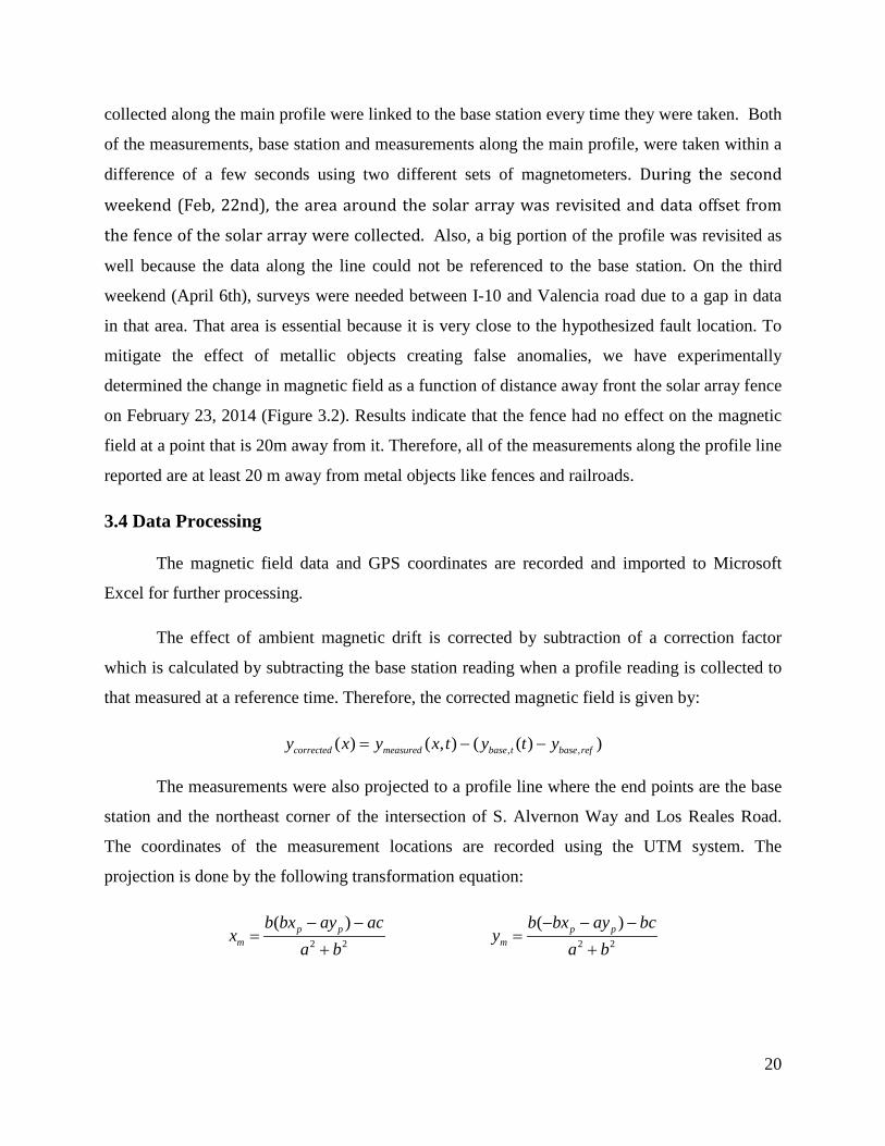
mitigate the effect of metallic objects creating false anomalies, we have experimentally

determined the change in magnetic field as a function of distance away front the solar array fence

on February 23, 2014 (Figure 3.2). Results indicate that the fence had no effect on the magnetic

field at a point that is 20m away from it. Therefore, all of the measurements along the profile line

reported are at least 20 m away from metal objects like fences and railroads.

3.4 Data Processing

The magnetic field data and GPS coordinates are recorded and imported to Microsoft

Excel for further processing.

The effect of ambient magnetic drift is corrected by subtraction of a correction factor

which is calculated by subtracting the base station reading when a profile reading is collected to

that measured at a reference time. Therefore, the corrected magnetic field is given by:

, ,( ) ( , ) ( ( ) )corrected measured base t base refy x y x t y t y= − −

The measurements were also projected to a profile line where the end points are the base

station and the northeast corner of the intersection of S. Alvernon Way and Los Reales Road.

The coordinates of the measurement locations are recorded using the UTM system. The

projection is done by the following transformation equation:

2 2 2 2

( ) ( )p p p pm m

b bx ay ac b bx ay bcx y

a b a b− − − − −

= =+ +

20

where ax+by+c = 0 is the equation representing a straight line which goes through (x1,y1) and

(x2,y2); (xp,yp) is the point where a measurement is taken; and (xm,ym) is the projected point on

the profile line.

Figure 3.3 shows the corrected and projected magnetic field profile. Each line represents

data collected on a particular day. A table is also included in Appendix A, which lists the raw

and corrected data.

3.5 Interpretation

From the results in Figure 3.4, we do not observe any significant anomalies that can

potentially be attributed to a fault. However, a regional anomaly was identified as the magnetic

field is found to decrease from NE to SW. There are also several short wavelength, small

amplitude fluctuations. Those are probably not attributed to faults. They are more likely to be

associated with anthropogenic features such as metal trash. The sampling spacing is between 50-

100m so that the spatial resolution is high enough to detect any anomalies of interest. Also, the

measured data used simultaneous measurements at the base station, which were used to correct

for any shift in the ambient magnetic field. In summary, the magnetic field data do not show

evidence of any fault in the study area.

3.6 Reference

Garmin International Inc. 2007. Owner’s Manual for Rino® 520-530HCx 2-way radio

and GPS.

U.S. Army Corps of Engineers. 1995. Geophysical Exploration for Engineering and

Environmental Investigations. USACE EM 1110-1-1802

21

Figure 3.1 Location map for magnetic field measurements.

000 300300300 1500

22

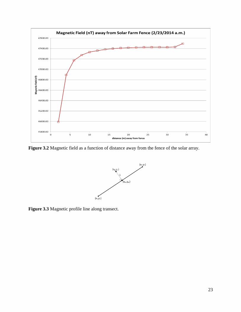
Figure 3.2 Magnetic field as a function of distance away from the fence of the solar array.

Figure 3.3 Magnetic profile line along transect.

23

Figure 3.4 Magnetic profile line along transect.

24

4. Gravity Survey 4.1 Introduction, Instrumentation and Data Collection

A gravity survey was conducted to investigate the possibility of gravity anomalies in the

study area that may be indicative of subsurface geological features. The gravity meter used in

this survey was a LaCoste Romberg model G-575. A designated pair of operators worked in

tandem for the duration of the survey. After a station was chosen and the meter was leveled,

operator A took and recorded a measurement, immediately followed by operator B, always in the

same order. The time was recorded along with GPS coordinates for each station. The first

recording station was designated the base station; repeat measurements were taken at the base

station every two hours to account for instrument drift.

4.2 Locations

An initial survey was made along the main NE-SW transect line of the study area. The

stations were located approximately 400m-600m apart depending on local obstacles, and

spanned the entire length of the study area diagonal. After analysis of this initial coarse survey, a

focus area was chosen between the solar array and the Interstate-10 (I-10). A second survey was

conducted there, consisting of three parallel survey lines: one along the main diagonal, and one

each 300m NW and SE of the central line (Figure 4.1). Stations were selected 100m apart down

all three lines. Station locations along the offset lines were projected orthogonally onto the main

transect for data analysis.

4.3 Data Processing

The gravity values recorded by each operator were averaged to produce a single

measurement value at each station. See Figure 4.2 for a complete table of raw measurements.

This combined value was then corrected for instrument drift, latitude, free-air and Bouguer

anomalies (Figure 4.3). Correction calculations were performed as per “An Introduction to

Geophysical Exploration”, Keary, Brooks, and Hill, 3rd ed, 6.8.3 (drift corr.) and 6.8.6 (free

air/Bouguer). These relative gravity anomaly data were then converted to absolute gravity using

a tie-in point in the Harshbarger/Mines building on the University of Arizona campus (1133 E

North Campus Dr, Tucson AZ 85721) where absolute gravity is known.

25

4.4 Results

The full length, coarse transect shows a regional gravitational gradient, steadily

decreasing from NE to SW, with a large anomaly apparent around 1500m from the base station,

between the railroad tracks and the I-10 (Figure 4.4). The central high-resolution line along the

main transect appears to repeat this anomaly; however, the offset lines show no repetition of such

an anomaly (Figure 4.5). Rather, they show very little change in value, indicating the anomaly

along the main transect is a local one, and not consistent with a NW-SE trending fault contact.

26

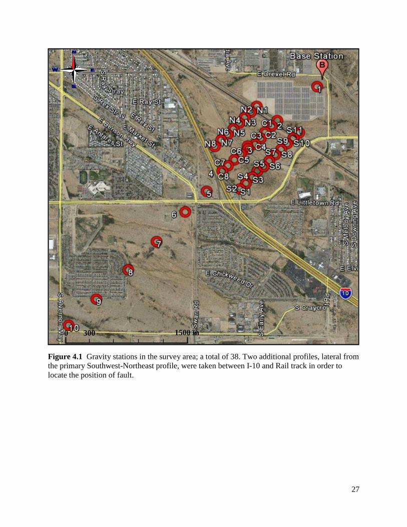
Figure 4.1 Gravity stations in the survey area; a total of 38. Two additional profiles, lateral from the primary Southwest-Northeast profile, were taken between I-10 and Rail track in order to locate the position of fault.

0 300 1500 m

27

Figure 4.2 Raw field data with GPS and time information.

28

Figure 4.3 Data processing spreadsheat.

29

Figure 4.4 All data plotted as absolute gravity values. Railroad and I-10 marked.

Figure 4.5 Zoom plot of the offset lines.

30

5. Passive-Seismic Survey 5.1 Introduction

Passive-seismic analysis is one of the methods used to analyze the subsurface structure of

the study area. The horizontal-to-vertical spectral ratio method (H/V) was used to interpret the

data. The H/V method relies on ambient seismic noise and can be used for estimating the

thickness of unconsolidated deposits. A change in the seismic properties of the subsurface is

shown as a peak in the H/V spectral ratio. This is the primary resonant frequency (shear wave)

of the overburden and an empirical relationship is used to determine the thickness from the

frequency.

Passive seismic analysis is an inexpensive and relatively fast method for obtaining

seismic data. It is limited by interference from human activity and works better in low-

population areas. Passive seismic analysis is intended to be a supplement to other geophysical

methods as was the case in this study.

5.2 Instrumentation and Field Procedures

The measurements were performed perpendicular to the postulated fault location. These

measurements started at the base station located near E. Drexel Rd and S. Craycroft Rd and were

collected along a line running southwest toward E. Los Reales Rd and S. Alvernon Way. Data

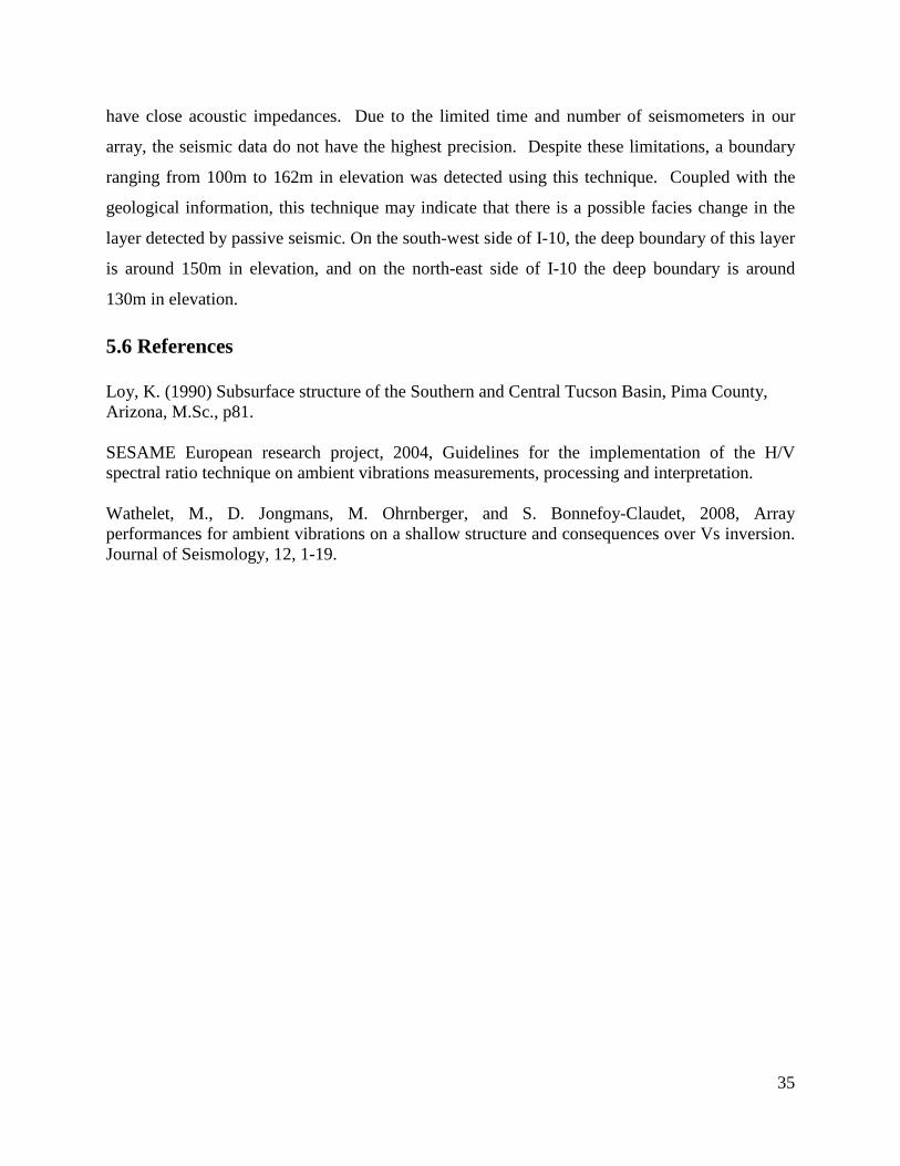
were also collected near an existing test well site. Figure 5.1 shows the locations where passive

seismic instruments were set up for data collection.

Three Guralp CMG-6TD seismometers were used in the study, the sensor IDs were

A834, B74 and B76. Table 5.1 shows the coordinates of each station corresponding to locations

in Figure 5.1. A gravity meter plate was used as a leveling plate everywhere except for the base

station (Figure 5.2). A tilted table was used in some cases in order to block some of the wind.

At the base station a shallow hole was dug for the seismometer and the seismometer was leveled

on the ground at the bottom of the hole. This method kept the equipment safer and reduced

interference caused by wind.

31

Site ID Sensor ID Easting Northing

Proj. Dist. From Base (m)

Elevation AMSL(m)

file(s)

Base

Station A834 511709.3 3556853 0 822.23 2014_1856-0000

Well DW-

9 B74 510420 3557722 295 808.63 20140222_1928-2000

1 B76 511172 3556351 735 816.92 20140222_2331_0000

2 B76 511008 3556183 970 816.42 20140222_2252-2300

3 B76 510817 3556024 1217 814.8 20140222_2007

4 B76 510688 3555896 1399 815.31 20140222_2152-2200

5 B74 510720 3555728 1496 816.42 20140316_2319

20140317_0000

6 B76 510511 3555721 1648 817.23 20140222_2100_57

7 B74 509665 3554905 2823 811.67 20140316_2128_2200

8 B74 509512 3554162 3260 816.48 20140222_2239

9 B74 508671 3553778 4024 811.39 20140222_2127

Table 5.1 Passive-seismic locations, seismometer Id#, projected distances from base station and the corresponding files created during data collection on 2/22/14 and 3/10/14.

5.3 Data and Results

The intended scheme for data collection was to retain proximity to the main profile line,

which runs northeast to southwest, more or less orthogonal to the postulated fault in the area.

This was adhered to in the northeastern region of the study area despite many structural

obstacles. In the southwest area of study it was somewhat more difficult, and therefore,

measurements are more disperse.

Once these data were collected and downloaded, a data-processing program called

Geopsy, (Wathelet et al., 2008) was used to identify the maximum sediment depth. Due to the

fact that often several files were created by the seismometer during data collection at a given site,

files were merged using Geopsy prior to data processing. Before the H/V spectral ratio can be

32

generated, it is necessary to consider the length of the time window. Based on the duration of

each site survey and the recommendations outlined by SESAME (2004), we selected a 50 second

window for the majority of the processing.

A major consideration when processing seismic data is the significant influence nearby

industrial noise can have on the interpretation of data. This is of particular importance because

much of the study area lies within a kilometer of a busy interstate and a railroad. The damping

tool in Geopsy can detect the frequency of local industrial noises (Fig. 5.3). For this reason, the

data were subsequently processed with two filters. A high-pass filter set to 0.9 Hz and a band-

reject filter set for a range of 0.9 – 1.1 Hz.

The frequency at the peak of the spectral ratio (f H/V ) is of primary interest to determine

the sediment thickness, depth to bedrock, (hmin ) using Equation 5.1. Shear wave velocity (vs )

can range from 300-12,000 ft/sec. Previous work in the Tucson Basin by Loy (1990) determined

the alluvium in this area to be 5500 feet/sec.

ℎ𝑚𝑚𝑚𝑚𝑚𝑚 = 𝑣𝑣𝑠𝑠4 𝑓𝑓𝐻𝐻/𝑉𝑉

5.1

Site ID Sensor

Proj. Dist. From Base

Station (m)

f H/V (Hz)

Amp. Of fH/V

Predicted elevation AMSL

(m)

Predicted Depth (m)

Base Station A834 0 0.594 2.89 117 706

Well DW-9 B74 295 0.597 10.03 106 702

1 B76 735 0.589 1.98 105 712 2 B76 970 0.609 5.48 128 689 3 B76 1217 0.606 2.30 123 692 4 B76 1399 0.613 8.66 132 684 5 B74 1496 0.591 2.13 107 709 6 B76 1648 0.612 2.78 132 685 7 B74 2823 0.622 1.76 137 674 8 B74 3411 0.640 3.55 160 655 9 B74 4321 0.590 4.10 100 711

Table 5.2 Passive-seismic locations and predicted depth to the deep boundary of the subsurface layer.

33

The peak frequency can be identified during the processing of the data once the spectra

are generated in Geopsy (Figs. 5.4-5.14). Results of these data are seen in Table 5.2 and Figures

5.15-17.

5.4 Data Interpretation

The H/V processing results of the passive seismic surveys have the primary peak fH/V at a

range from 0.5 to 0.7Hz (Table 5.2). For most cases, we can clearly see this peak and get the fH/V.

The amplitudes of these peaks range from 1.7 to 10.0 (Table 5.2). However, there aren’t obvious

secondary peaks. This makes it difficult to predict boundary depths for other layers. Thus, from

our processing results, we can only detect a deep layer boundary. This boundary is much deeper

than the results from the TEM method. The final processing results of the H/V are shown in

Figures 5.15-5.17.

In Figure 5.17 we see that the calculated elevations (AMSL) of the ten stations are highly

variable. On the north-east side of I-10, elevations are from 105m to 132m, typically close to

130m. Elevations predicted on the south-west side of I-10, range from 100m to 162m. It is

possible that the variations in the elevation of this boundary represent a facies change rather than

an offset due to a fault. The drop in predicted elevation at the location 1495m from the base

station (Station 5) is significant relative to the nearby stations, which may be caused by nearby

noise. This can be seen from a smaller fH/V produced by the high-pass filter than the band-reject

filter (Figure 5.15). Though the noise effect is also seen in the last station, the drop at this station

may indicate a fault offset in this area. Unfortunately, we have only one station at this area and it

is not possible to predict detailed variations around this station. In general, the underground

layer detected by the passive-seismic survey has identified a boundary increasing from north-east

to south-west. A possible reason for this is that a facies change defines the depth of this deep

layer.

5.5 Discussion and Conclusion

One of the possible reasons why only one boundary is found is because the H/V

technique is effective when there is a large acoustic impedance contrast. If the underground

layers are very similar in acoustic impedance, it is difficult to find a peak in the H/V plot. Thus,

we can only see the deep boundary using the passive-seismic method, since the shallow layers

34

have close acoustic impedances. Due to the limited time and number of seismometers in our

array, the seismic data do not have the highest precision. Despite these limitations, a boundary

ranging from 100m to 162m in elevation was detected using this technique. Coupled with the

geological information, this technique may indicate that there is a possible facies change in the

layer detected by passive seismic. On the south-west side of I-10, the deep boundary of this layer

is around 150m in elevation, and on the north-east side of I-10 the deep boundary is around

130m in elevation.

5.6 References

Loy, K. (1990) Subsurface structure of the Southern and Central Tucson Basin, Pima County, Arizona, M.Sc., p81. SESAME European research project, 2004, Guidelines for the implementation of the H/V spectral ratio technique on ambient vibrations measurements, processing and interpretation. Wathelet, M., D. Jongmans, M. Ohrnberger, and S. Bonnefoy-Claudet, 2008, Array performances for ambient vibrations on a shallow structure and consequences over Vs inversion. Journal of Seismology, 12, 1-19.

35

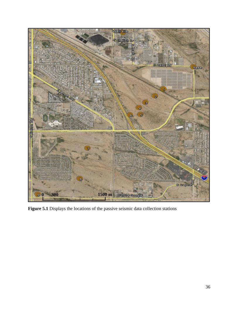
Figure 5.1 Displays the locations of the passive seismic data collection stations

0 300 1500 m

36

Figure 5.2 Seismometer in the field taking measurements. The battery is housed in the cooler.

37

Figure 5.3 The damping tool identifies the frequency at which industrial noise is detected. These results are from Site 1, which lies between the solar array and railroad tracks, show an industrial source at 0.22 Hz decaying at a rate of 3.44% per sec and at 1Hz decaying at a rate of 2.17% per sec. The damping tool was applied to all passive-seismic survey sites.

38

Figure 5.4 Processing results of Base Station. (a) H/V processing results, and (b) H/V rotate analysis, indicating an around 0.6Hz seismic source which seems to come in all directions and concentrates from 0 degree to 70 degree and from 140 degree to 180 degree.

Figure 5.5 Processing results of Station 1. (a) H/V processing results, and (b) H/V rotate analysis, indicating an around 0.6Hz seismic source which seems to come in all directions and concentrates from 0 degree to 80 degree and from 140 degree to 180 degree. The source around 1Hz and 20Hz are noise, we don’t use them.

(a) (b)

(a) (b)

39

Figure 5.6 Processing results of Station 2. (a) H/V processing results, and (b) H/V rotate analysis, indicating an around 0.6Hz seismic source which seems to come in all directions. The source around 1Hz is noise, we don’t use it.

Figure 5.7 Processing results of Station 3. (a) H/V processing results, and (b) H/V rotate analysis, indicating an around 0.6Hz seismic source which seems to come in directions from 30 degree to130 degree. The source around 1Hz and 20Hz are noise, we don’t use them.

(a) (b)

(a) (b)

40

Figure 5.8 Processing results of Station 4. (a) H/V processing results, and (b) H/V rotate analysis, indicating an around 0.6Hz seismic source which seems to come in directions from 50 degree to180 degree. The source around 1Hz is noise, we don’t use it.

Figure 5.9 Processing results of Station 5. (a) H/V processing results, and (b) H/V rotate analysis, indicating an around 0.6Hz seismic source which seems to come in directions from 110 degree to180 degree. The source around 0.2Hz is noise, we don’t use it.

(a) (b)

(a) (b)

41

Figure 5.10 Processing results of Station 6. (a) H/V processing results, and (b) H/V rotate analysis, indicating an around 0.6Hz seismic source which seems to come in all directions. The sources around 1Hz and 15Hz are noise, we don’t use them.

Figure 5.11 Processing results of Station 7. (a) H/V processing results, and (b) H/V rotate analysis, indicating an around 0.6Hz seismic source which seems to come in all directions. The sources around 0.2Hz and 20Hz are noise, we don’t use them.

(a) (b)

(a) (b)

42

Figure 5.12 Processing results of Station 8. (a) H/V processing results, and (b) H/V rotate analysis, indicating an around 0.6Hz seismic source which seems to come in all directions. The sources around 2Hz and 20 Hz are noise, we don’t use them.

Figure 5.13 Processing results of Station 9. (a) H/V processing results, and (b) H/V rotate analysis, indicating an around 0.6Hz seismic source which seems to come in directions from 0 degree to 40 degree and from 120 degree to 180 degree. The source around 0.2Hz is noise, we don’t use it.

(a) (b)

(a) (b)

43

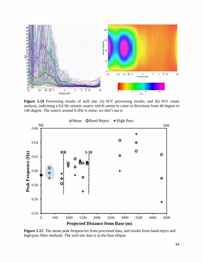
Figure 5.14 Processing results of well site. (a) H/V processing results, and (b) H/V rotate analysis, indicating a 0.6 Hz seismic source which seems to come in directions from 40 degree to 140 degree. The source around 0.2Hz is noise, we don’t use it.

Figure 5.15 The mean peak frequencies from processed data, and results from band-reject and high-pass filter methods. The well site data is in the blue ellipse.

0.54

0.56

0.58

0.60

0.62

0.64

0.66

0 500 1000 1500 2000 2500 3000 3500 4000 4500

Peak

Fre

quen

cy (H

z)

Projected Distance from Base (m)

Mean Band Reject High Pass

RR I-10

NE SW

44

Figure 5.16 The processing results (averaged from both filtering processes) of the passive seismic profile. The data in blue are from the well site, DW-9.

-720

-710

-700

-690

-680

-670

-660

-650

0.58

0.59

0.6

0.61

0.62

0.63

0.64

0.65

0 500 1000 1500 2000 2500 3000 3500 4000 4500

Pred

icte

d D

epth

(m)

Peak

Fre

quen

cy (H

z)

Projected Distance from Base (m)

Pk freq. Depth

RR I-10

NE SW

45

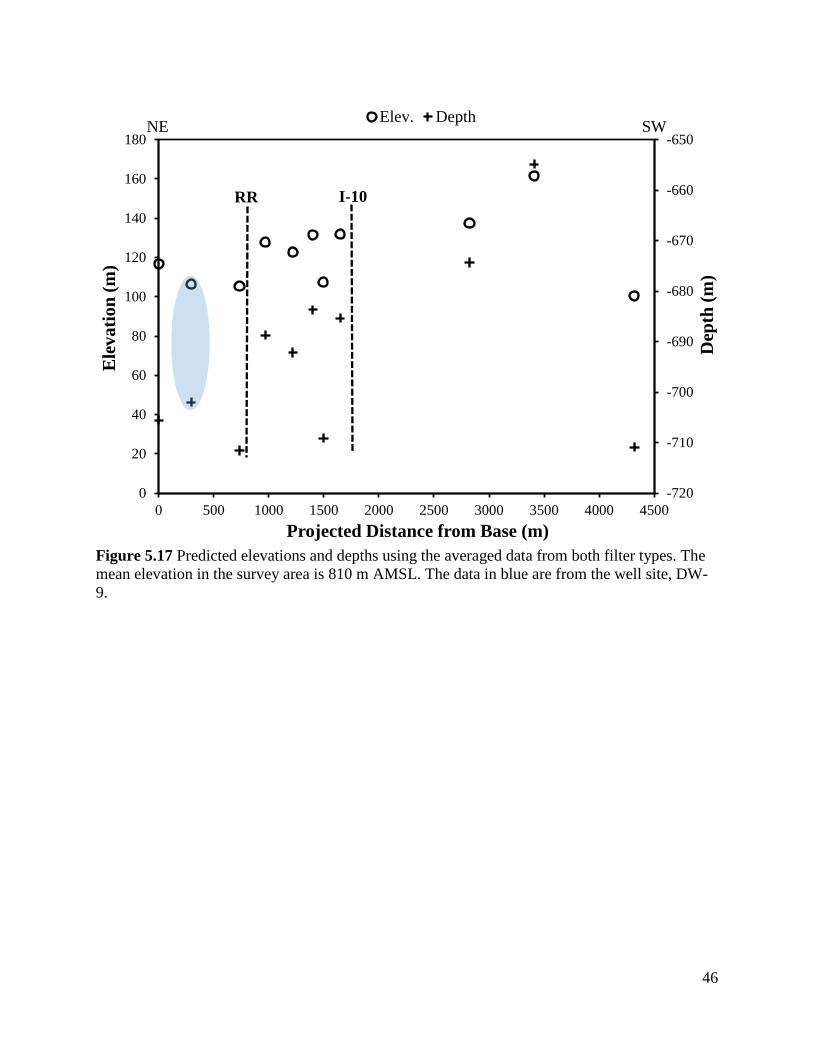
Figure 5.17 Predicted elevations and depths using the averaged data from both filter types. The mean elevation in the survey area is 810 m AMSL. The data in blue are from the well site, DW-9.

-720

-710

-700

-690

-680

-670

-660

-650

0

20

40

60

80

100

120

140

160

180

0 500 1000 1500 2000 2500 3000 3500 4000 4500

Dep

th (m

)

Ele

vatio

n (m

)

Projected Distance from Base (m)

Elev. Depth

RR I-10

NE SW

46

6. Transient Electromagnetic Survey 6.1 Introduction

Transient Electromagnetic (TEM) is a geophysics method that is widely used for

mapping subsurface layers. In this project, the TEM method was used to investigate depth to

layers and depth to water table in the survey area. Generally, the maximum exploration depth of

the TEM central-loop induction method is about 2 to 3 times the loop size. For more information

about the TEM method, see the paper “Introduction to TEM” (Zonge, 2009). A total of eight

sites were recorded within two days for this project. A postulated fault is located northeast of

Interstate 10 (I-10) and we are trying to find which side of the fault is higher, so data were

collected by setting four loops on each side of Interstate 10 (I-10). The transmitter loop sites

were 200m X 200m.

6.2 Locations

The TEM data were recorded at eight sites in the Tucson Basin. On 3-1-2014, only two

loops were measured, loop 1 and loop 2. On the second day 3-2-2014, another 6 loops were

measured. For loop 6, a homeless camp was at the initial planned location, so it had to be shifted

about 300m southwest of that location. Loop 1, 2, 7 and 8 are at on the northeast side of I-10.

Loop 3, 4, 5 and 6 are at on the southwest side of I-10. Because of the existence of the solar array

(northeast corner of the survey area) and the subdivision (southwest corner of the survey area),

we cannot put a 200m x 200m loop there, and small loops cannot give us the depth needed, so

there are no measurements in those two areas. The locations of eight loops are shown in Figure

6.1.

47

Figure 6.1 TEM survey stations. The loop size for TEM survey is 200m × 200m. There are 8 loops in the survey area.

6.3 Instrumentation and Field procedures.

The TEM equipment for these measurements includes the GDP 32II multi-function

receiver (Zonge 2012), the ZT-30 TEM transmitter (Zonge, 2013a) and the XMT-32S transmitter

controller (Zonge, 2013b). The XMT-32S transmitter controller controls ZT-20 TEM transmitter

to generate 8Hz and 16Hz square waves into a 200m x 200m loop. The GDP 32II multi-function

0 300 1500m

48

receiver is connected to a vertical magnetic-field sensor at the center of the loop. The receiver

measures the off-time signal, which can be used to obtain the resistivity information of the earth.

The GDP 32II multi-function receiver must first be synchronized with the XMT-32S transmitter

controller before measurements. A current of 2.2Amps was used in these measurements. Two

12-VDC batteries were connected in series to provide the power to the transmitter.

We tried to keep the transmitter loop as square as possible and away from fences, the rail-

tracks, the solar array, and the subdivision. We used GPS to measure the distance between loop

corners. After loop set up, we calculated the center position and then acquired our measurements

at that location.

6.4 Data Processing

After TEM data were obtained in the field, we downloaded the data from the GDP 32II to

a computer. The raw data were sorted and organized and then processed using Zonge

International’s proprietary suite of software called DATPRO. Then, the data were trimmed or

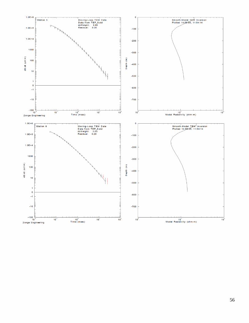
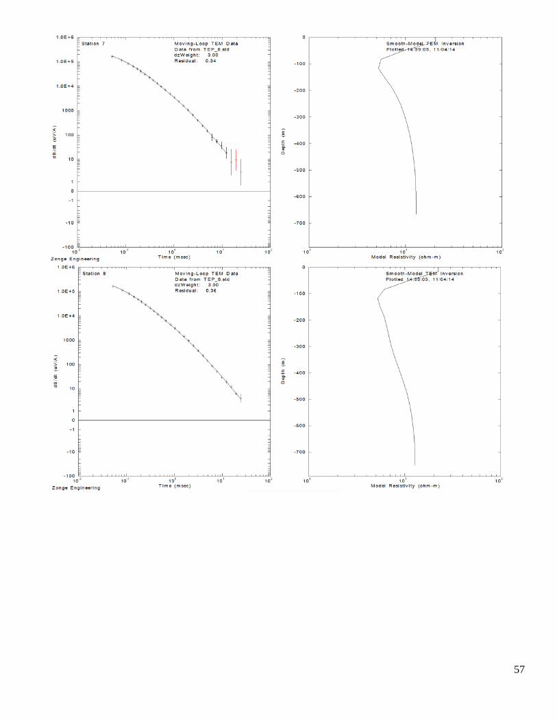
edited for data that were inconsistent with the overall decay curve. The data were then inverted

by the Zonge STEMINV inversion program, using the smooth-inversion method (MacInnes and

Raymond, 2009). We finally obtained a smooth layered-earth model for each station. The one-

dimensional inversion results are shown in Appendix B. The measured decay curve is compared

with the best-fit calculated decay curve. The solid line is the best-fit decay curve and the plus

symbol line is the measured decay curve. The red plus symbols are time windows not used in the

calculation. The one-dimensional earth models are shown on the right side of each plot.

6.5 TEM processing results.

With the inversion results from STEMINV, we plotted 2D cross sections. We used

Golden Software’s Surfer 11 to display the inversion data. The gridding method we used was the

Kriging method. Because we only have 8 stations in total, and the separation is quite large

between the stations on the NE and the stations on the SW, the results in the middle of the cross

section are not reliable. Thus, in the contour plots, we blanked that area. For these 8 stations, we

divided the data into two lines, the north line and the south line. Each line has 4 loops. With 8Hz

49

and 16Hz, we have 4 contour plots, as shown in Figure 6.2 to Figure 6.5. We projected the loop

locations to the main profile lines.

6.6 Interpretation

Based on the four TEM-model contour plots, both sides of the profiles have a very low

resistivity region below the more resistive surface layers. On the northeast side of I-10, the low-

resistivity region starts around 750m in elevation and continues very deep. On the southwest

side, this region starts around 720m in elevation and continues very deep. This low-resistivity

region is likely caused by high TDS in the water and high shale content. Referring to the

hydrogeologic cross section (Figure 1.5), the top of these low-resistivity areas is in the area of

the water-table depth. Another important feature from these contour plots relates to the offset in

the top boundary of these low-resistivity regions. Using the same resistivity contour line, the

northeast side of I-10 is always shallower than the southwest side of I-10. All four plots contain

this feature (Figures 6.2, 6.3, 6.4, 6.5). This feature indicates the water table on the northeast side

of I-10 is shallower thn that on the southwest side of I-10.

The 8Hz pulse repetition frequency has a somewhat deeper depth of investigation than

the 16 Hz. From the 8Hz contour plots (Figures 6.2, and 6.3), the deep resistivities also show an

offset.

Resistivity well-log information from DW-9 (Figure 6.6), shows a resistivity increase

using the 16 and 64 inch normal resistivity tools, starting at 1400 ft (427m) depth, and increasing

more at 1800 ft (549m) depth, till the end of the well log at 2200 ft (671m) depth. The resistivity

increase around 400m in elevation on the left side of Figures 6.2 and 6.3 is similar to the

resistivity increase around 1400 ft (427m) depth in Figure 6.6. From the 8Hz contour plots

(Figures 6.2 and 6.3), the deep boundary of the low-resistivity regions also show a change in

elevation along the profile. For example, the 12 ohm-m contour line is around 400m on the left

side of Figures 6.2 and 6.3, but on the right side it is much deeper. It is possible that the

variations in this deep boundary are due to facies changes across the section, rather than an offset

due to faulting.

50

6.7 References Maclnnes S., Raymond M., 2009, Zonge Data processing smooth-model TEM inversion. Zonge International. Zonge, 2009. Introduction to TEM. (http://www.zonge.com.au/docs/tem/intro_tem.pdf) Zonge, 2012. GDP-32II. Geophysical receiver. Multi-function receiver.

(http://www.zonge.com/legacy/PDF_Equipment/Gdp-32ii.pdf)

Zonge, 2013a, ZT-30 Geophysical transmitter.

(http://www.zonge.com/legacy/PDF_Equipment/Zt-30.pdf)

Zonge, 2013b, XMT-32S Transmitter Controller.

(http://www.zonge.com/legacy/PDF_Equipment/Xmt-32s.pdf)

51

Figure 6.2 Cross section of 8Hz TEM data inversion results at the north line. Between loop 7 and loop 3, the no-data region is interpolated by Surfer, which is not reliable, so we blanked this area. The locations are projected to the main profile for better comparison.

Figure 6.3 Cross section of 8Hz TEM data inversion results at the south line. With the same reason in Figure 6.2, we blanked them. The locations are projected to the main profile for better comparison.

6

7

8

8

8

9

9

9

10

10

10

1011

11

11

11

12

12

12

12

13

13

13

14

14

14

15

15

15

16

16

16

17

17

18

18

19

19202122

1200 1400 1600 1800 2000 2200 2400 2600 2800 3000

Loop Projected Location (m)

300

400

500

600

700

800

eat

o (

)S

Loop 1 7 3

0

7

7

8

8

8

8

9

9

9

9

9

10

10

10

10

11

1111

11

12

12

12

12

13

13

13

13

14

14

14

15

1515

16

16

16

17

17

17

18

18

19

1920

20 2122

1200 1400 1600 1800 2000 2200 2400 2600 2800 3000 3200

Loop Projected Location (m)

300

400

500

600

700

800

eat

o (

)

Loop 2 8 4

S0

52

Figure 6.4 Cross section of 16Hz TEM data inversion results at the north line. With the same reason in Figure 6.2, we blanked them. The locations are projected to the main profile for better comparison.

Figure 6.5 Cross section of 16Hz TEM data inversion results at the south line. With the same reason in Figure 6.2, we blanked them. The locations are projected to the main profile for better comparison.

89

9

10

10

10

11

11

11

1212 1313 14

14

15

15

16

16

17

17

18

18

19

19

2021

1200 1400 1600 1800 2000 2200 2400 2600 2800 3000

Loop Projected Location (m)

400

500

600

700

800

eat

o (

)

Loop 1 7 3

S0

9

9

10

1010

10

11

11

11

11

12

12

12

13

1313

14

1414

15

1515

16

16

16

17

17

18

18

19

19

2021

1200 1400 1600 1800 2000 2200 2400 2600 2800 3000 3200

Loop Projected Location (m)

400

500

600

700

800

eat

o (

)

Loop 2 8 4

S0

53

(a)

54

(b)

55

(c)

56

Figure 6.6 Partial information of Well-log DW-9. 16" normal resistivity and 64" normal resistivity oscillate from 50 (15m) to 200 ft (61m) at shallow depth and increase after 1400 ft. Single point resistance has the same pattern.

(d)

57

Appendix A: Magnetic Field Data April 6 2014 Data:

Projected

distance from Base

Uncorrected Reading (nT)

base reading

longitude 12S

latitude projected x

projected y correction corrected reading

MC-1 2085.965005 47318.79 47408.8 510209 3555403 510234 3555378 -35.3 47354.09 MC-2 2037.881743 47337.91 47407.2 510243 3555437 510268 3555412 -36.9 47374.81 MC-3 1986.970055 47330.98 47408.2 510280 3555472 510304 3555448 -35.9 47366.88 MC-4 1936.058367 47335.05 47409.2 510316 3555508 510340 3555484 -34.9 47369.95 MC-5 1886.560892 47335.29 47408.6 510351 3555543 510375 3555519 -35.5 47370.79 MC-6 1837.063418 47334.45 47408 510387 3555577 510410 3555554 -36.1 47370.55 MC-7 1316.632827 47369.78 47408.7 510757 3555943 510778 3555922 -35.4 47405.18 MC-8 1382.393757 47352.2 47406.1 510707 3555900 510731.5 3555876 -38 47390.2 MC-9 1435.426766 47359.41 47405.4 510671 3555861 510694 3555838 -38.7 47398.11 MC-10 1486.338454 47345.49 47404.4 510637 3555823 510658 3555802 -39.7 47385.19 MC-11 1536.543036 47347.51 47404.8 510599 3555790 510622.5 3555767 -39.3 47386.81 MC-12 1587.454724 47347.37 47405 510565 3555752 510586.5 3555731 -39.1 47386.47 MC-13 1636.245092 47333.85 47405.2 510529 3555719 510552 3555696 -38.9 47372.75 MC-14 1611.496354 47350.32 47406.2 510545 3555738 510569.5 3555714 -37.9 47388.22 MC-15 1624.224276 47344.38 47406.2 510538 3555727 510560.5 3555705 -37.9 47382.28

50

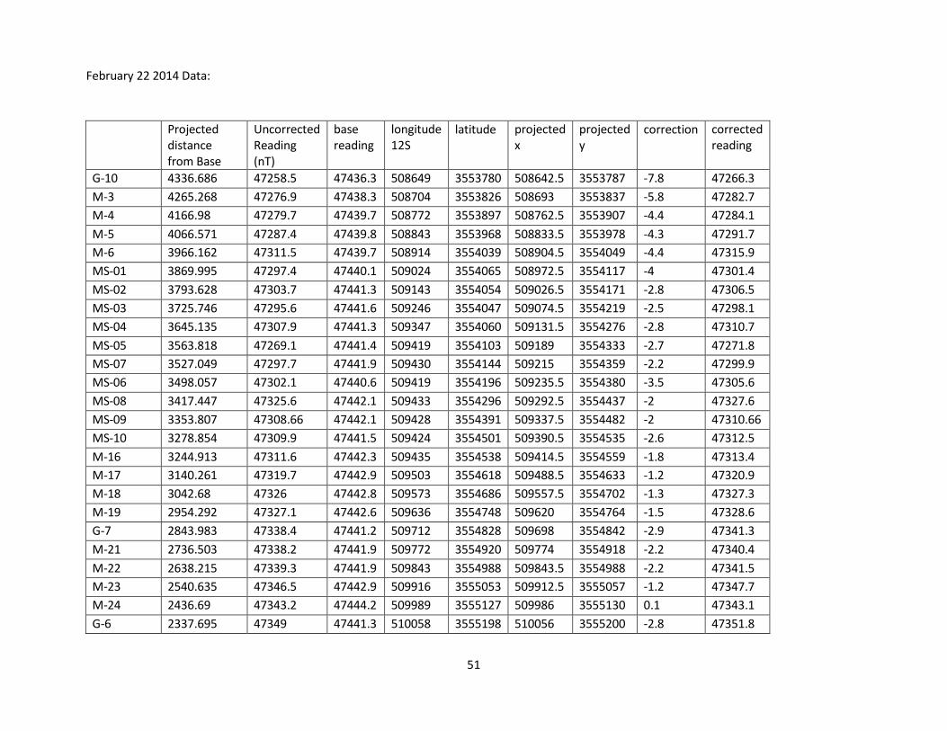
February 22 2014 Data:

Projected distance from Base

Uncorrected Reading (nT)

base reading

longitude 12S

latitude projected x

projected y

correction corrected reading

G-10 4336.686 47258.5 47436.3 508649 3553780 508642.5 3553787 -7.8 47266.3 M-3 4265.268 47276.9 47438.3 508704 3553826 508693 3553837 -5.8 47282.7 M-4 4166.98 47279.7 47439.7 508772 3553897 508762.5 3553907 -4.4 47284.1 M-5 4066.571 47287.4 47439.8 508843 3553968 508833.5 3553978 -4.3 47291.7 M-6 3966.162 47311.5 47439.7 508914 3554039 508904.5 3554049 -4.4 47315.9 MS-01 3869.995 47297.4 47440.1 509024 3554065 508972.5 3554117 -4 47301.4 MS-02 3793.628 47303.7 47441.3 509143 3554054 509026.5 3554171 -2.8 47306.5 MS-03 3725.746 47295.6 47441.6 509246 3554047 509074.5 3554219 -2.5 47298.1 MS-04 3645.135 47307.9 47441.3 509347 3554060 509131.5 3554276 -2.8 47310.7 MS-05 3563.818 47269.1 47441.4 509419 3554103 509189 3554333 -2.7 47271.8 MS-07 3527.049 47297.7 47441.9 509430 3554144 509215 3554359 -2.2 47299.9 MS-06 3498.057 47302.1 47440.6 509419 3554196 509235.5 3554380 -3.5 47305.6 MS-08 3417.447 47325.6 47442.1 509433 3554296 509292.5 3554437 -2 47327.6 MS-09 3353.807 47308.66 47442.1 509428 3554391 509337.5 3554482 -2 47310.66 MS-10 3278.854 47309.9 47441.5 509424 3554501 509390.5 3554535 -2.6 47312.5 M-16 3244.913 47311.6 47442.3 509435 3554538 509414.5 3554559 -1.8 47313.4 M-17 3140.261 47319.7 47442.9 509503 3554618 509488.5 3554633 -1.2 47320.9 M-18 3042.68 47326 47442.8 509573 3554686 509557.5 3554702 -1.3 47327.3 M-19 2954.292 47327.1 47442.6 509636 3554748 509620 3554764 -1.5 47328.6 G-7 2843.983 47338.4 47441.2 509712 3554828 509698 3554842 -2.9 47341.3 M-21 2736.503 47338.2 47441.9 509772 3554920 509774 3554918 -2.2 47340.4 M-22 2638.215 47339.3 47441.9 509843 3554988 509843.5 3554988 -2.2 47341.5 M-23 2540.635 47346.5 47442.9 509916 3555053 509912.5 3555057 -1.2 47347.7 M-24 2436.69 47343.2 47444.2 509989 3555127 509986 3555130 0.1 47343.1 G-6 2337.695 47349 47441.3 510058 3555198 510056 3555200 -2.8 47351.8

51

M-26 2271.227 47357.9 47440.4 510118 3555232 510103 3555247 -3.7 47361.6 MN29 1224.002 47405 47432 510827 3556004 510843.5 3555988 -12.1 47417.1 MN28 1196.425 47389.6 47432.8 510866 3556004 510863 3556007 -11.3 47400.9 MN27 1147.634 47396.3 47432.6 510887 3556052 510897.5 3556042 -11.5 47407.8 MN26 1095.308 47385.4 47432.8 510937 3556076 510934.5 3556079 -11.3 47396.7 MN25 1029.547 47391.2 47430.7 510966 3556140 510981 3556125 -13.4 47404.6 MN24 999.1419 47394.3 47430.7 511005 3556144 511002.5 3556147 -13.4 47407.7 MN23 946.1089 47392.3 47431 511047 3556177 511040 3556184 -13.1 47405.4 MN22 893.783 47383.1 47431 511079 3556219 511077 3556221 -13.1 47396.2 MN21 816.7083 46839 47431.5 511140 3556267 511131.5 3556276 -12.6 46851.6 MN20 702.8641 47402.2 47431.7 511250 3556318 511212 3556356 -12.4 47414.6 MN19 661.8519 47394.2 47430.8 511302 3556324 511241 3556385 -13.3 47407.5 MN18 627.2037 47391.7 47432.1 511352 3556323 511265.5 3556410 -12 47403.7 MN17 591.1413 47401.9 47430.5 511402 3556324 511291 3556435 -13.6 47415.5 MN16 555.7859 47398.3 47430.7 511455 3556321 511316 3556460 -13.4 47411.7 MN15 518.3093 47411.7 47430.1 511508 3556321 511342.5 3556487 -14 47425.7 MN14 485.0753 47408.4 47429.1 511558 3556318 511366 3556510 -15 47423.4 MN13 439.8204 47414.7 47429.9 511606 3556334 511398 3556542 -14.2 47428.9 MN12 385.3732 47411.8 47430 511651 3556366 511436.5 3556581 -14.1 47425.9 MN11 347.8965 47425.3 47430.1 511701 3556369 511463 3556607 -14 47439.3 MN10 306.1772 47415.9 47432.5 511750 3556379 511492.5 3556637 -11.6 47427.5 MN9 254.5584 47369.7 47432.9 511756 3556446 511529 3556673 -11.2 47380.9 MN8 219.9102 47385.9 47431.5 511756 3556495 511553.5 3556698 -12.6 47398.5 MN7 183.8478 47406.2 47433.4 511757 3556545 511579 3556723 -10.7 47416.9 MN6 146.3711 47408.4 47433.4 511759 3556596 511605.5 3556750 -10.7 47419.1 MN5 110.3087 47416 47435.4 511760 3556646 511631 3556775 -8.7 47424.7 MN2 96.16652 47422.5 47434.6 511649 3556777 511641 3556785 -9.5 47432 MN4 76.36753 47382.3 47434.4 511758 3556696 511655 3556799 -9.7 47392 MN1 70.71068 47437.4 47436.2 511667 3556795 511659 3556803 -7.9 47445.3 MN3 48.08326 47407.4 47433.8 511749 3556745 511675 3556819 -10.3 47417.7

52

February 8 2014 Data:

Projected

distance from Base

Uncorrected Reading (nT)

base reading

longitude 12S

latitude projected x

projected y correction corrected reading

90.5 47395.68 47416.8 511667 3556795 N/A N/A -27.30 47422.98 M-35 877.44 47367.16 47430.4 511070 3556253 -13.70 47380.86 M-34 950.19 47393.16 47432.2 510960 3556154 -11.90 47405.06 M-33 1026.94 47383.92 47431.4 510960 3556154 -12.70 47396.62 M-32 1124.41 47387.81 47426.5 510886 3556087 -17.60 47405.41 M-31 1223.76 47382.67 47434.6 510811.71 3556021.14 -9.50 47392.17 M-30 1253.35 47388.34 47434.5 510764 3555973 -9.60 47397.94 M-29 1325.01 47380.38 47436.4 510671 3555878 -7.70 47388.08 M-28 1424.24 47369.60 510505.52 3555709.84 47369.60

53

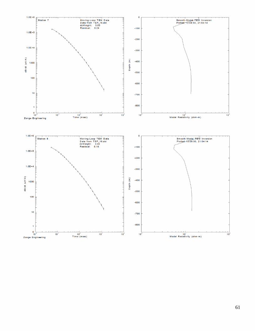
Appendix B: TEM Data Fits and Models

In this appendix, we show the smooth-model TEM inversion results for all the loops. The left sides of the figures display the measured decay curve with the best-fit calculated decay curve. The right sides of the figures show the inverse one-dimensional earth model for each station.

For 8Hz data

54

55

56

57

For the 16Hz data

58

59

60

61