University of Calgary

PRISM: University of Calgary's Digital Repository

Graduate Studies The Vault: Electronic Theses and Dissertations

2014-09-23

Geophysical Characterization of an Undrained Oil

Sands Tailings Pond Dyke Alberta, Canada

Booterbaugh, Aaron

Booterbaugh, A. (2014). Geophysical Characterization of an Undrained Oil Sands Tailings Pond

Dyke Alberta, Canada (Unpublished master's thesis). University of Calgary, Calgary, AB.

doi:10.11575/PRISM/26292

http://hdl.handle.net/11023/1788

master thesis

University of Calgary graduate students retain copyright ownership and moral rights for their

thesis. You may use this material in any way that is permitted by the Copyright Act or through

licensing that has been assigned to the document. For uses that are not allowable under

copyright legislation or licensing, you are required to seek permission.

Downloaded from PRISM: https://prism.ucalgary.ca

UNIVERSITY OF CALGARY

Geophysical Characterization of an Undrained Oil Sands Tailings Pond Dyke Alberta, Canada

by

Aaron Booterbaugh

A THESIS SUBMITTED TO THE FACULTY OF GRADUATE STUDIES

IN PARTIAL FULFILLMENT OF THE REQUIREMENTS FOR THE

DEGREE OF MASTER OF SCIENCE

DEPARTMENT OF GEOSCIENCE

CALGARY, ALBERTA

SEPTEMBER, 2014

© Aaron Booterbaugh 2014

ii

Abstract

Geophysical characterization of an undrained oil sands tailings pond dyke was conducted

at Syncrude Canada’s Southwest Sand Storage Facility (SWSS). Push tool conductivity

(PTC), electromagnetic (EM), and electrical resistivity tomography (ERT) methods in

conjunction with hydrogeological and chemistry measurements were used to investigate

soil moisture, hydraulic head, and groundwater salinity distributions. Normalization and

calibration procedures were conducted on EM data to build statistically consistent maps

between survey years. An Archie’s Law petrophysical model was utilized to relate

measured bulk conductivity, from geophysical surveying, with measures of soil moisture

and fluid electrical conductivity. It was found that a relatively strong relationship

between bulk electrical conductivity and soil moisture exists, while weak to no

correlation was observed between bulk and fluid electrical conductivity. ERT surveying

was capable of clearly identifying the location of the water table within the dyke. This

study provides a unique look into the application of geophysical techniques to investigate

soil moisture, hydraulic head, and salt distribution in an active undrained tailings dam

structure.

iii

Acknowledgements

I would first like to thank Dr. Larry Bentley and Dr. Carl Mendoza for their unwavering

support throughout my time at the University of Calgary, as well as with the project

presented in this manuscript.

My project was made possible through data provided by Dr. Carl Mendoza, Syncrude

Canada Ltd., and WorleyParsons Ltd. Specifically I would like to thank Mr. Paul

Bauman and Dr. Carl Mendoza for locating and delivering geophysical and

hydrogeological data, some of which collected over 10 years ago.

I would also like to thank my officemates for their help with navigating my degree and

project; Mike Callaghan, Lei Zhi, Frank Head, Amir Niazi, Sasha Zheltikova.

Finally, thanks to the University of Calgary and the Department of Geoscience.

iv

Table of Contents

Chapter 1: Introduction ................................................................................................... 1

1.1 Alberta Oil Sands .................................................................................................... 1

1.2 Study Site: Syncrude’s Southwest Sand Storage Facility ....................................... 3

1.3 Parameters of Interest and Petrophysical Model .................................................... 5

1.4 Geophysical Methods.............................................................................................. 7

1.4.1 Push Tool Conductivity ................................................................................... 7

1.4.2 Electromagnetic Surveying .............................................................................. 8

1.4.3 Electrical Resistivity Tomography ................................................................ 10

1.5 Hydrogeological Methods ..................................................................................... 13

1.5.1 Neutron Probe and Soil Moisture .................................................................. 13

1.5.2 Groundwater Sampling .................................................................................. 14

1.6 Purpose and Scope ................................................................................................ 15

1.7 Study Objectives ................................................................................................... 16

1.8 Contribution of Authors ........................................................................................ 16

1.9 References ............................................................................................................. 18

Chapter 2: Geophysical characterization of an undrained dyke containing an oil-

sands tailings pond, Alberta, Canada ........................................................................... 31

2.1 Introduction ........................................................................................................... 31

2.2 Study Site: Syncrude’s Southwest Sand Storage Facility ..................................... 34

2.3 Petrophysical Model ............................................................................................. 35

2.4 Materials and Methods .......................................................................................... 35

2.4.1 Data Acquisition ............................................................................................ 35

2.4.3 Push Tool Conductivity ................................................................................. 37

2.4.4 Electromagnetic Methods .............................................................................. 39

2.4.5 Electrical Resistivity Tomography ................................................................ 41

v

2.6 Discussion ............................................................................................................. 46

2.7 Conclusions ........................................................................................................... 52

2.8 References ............................................................................................................. 54

Chapter 3: Summary and Conclusions ......................................................................... 71

3.1 Summary ............................................................................................................... 71

3.2 Conclusions ........................................................................................................... 72

3.3 Future Work .......................................................................................................... 74

Appendix A: Push Tool Conductivity Figures & Data ............................................... 72

Appendix B: EM-38 Data ........................................................................................... 85

Appendix C: Electrical Resistivity Tomography Figures & Data .............................. 86

Appendix D: Volumetric Moisture from Neutron Probe Figures & Data .................. 91

Appendix E: Water Level Data .................................................................................. 99

Appendix F: Fluid Electrical Conductivity Data ..................................................... 100

Appendix G: EM-38 Normalization MATLAB Script ............................................. 101

Appendix H: Automated Layer Modeling Program for 1D Data in MATLAB ....... 103

vi

List of Tables

Table 2.1. Summary statistics for normalization example displayed in Figure 3. EM regions are labeled in the same fashion (regions X, Y, & Z) as seen in Figure 3. ............ 57 Table 2.2. Manually optimized inversion parameters selected for ERT modeling. ......... 58

vii

List of Figures and Illustrations

Figure 1.1. Alberta oil sand deposits. Taken from (Government of Alberta 2013). ......... 22 Figure 1.2.General location and satellite image of the SWSS facility. ............................. 23 Figure 1.3. Schematic of PTC probe (left) and photograph of truck mounted rig for PTC implementation (right) at the SWSS facility. Schematic adapted from (Schulmeister 2003). Photograph from (Komex 2001). ........................................................................... 24 Figure 1.4. Common electrode arrays and geometric factors utilized in EC probes, as well as ER surveys. Adapted from (Reynolds 2011). ............................................................... 25 Figure 1.5. Photograph of the EM-38 device (top right) and photographs of EM-38 surveying with use of an ATV, conducted at the SWSS facility (Komex 2001). ............. 26 Figure 1.6. Response functions for EM-38 device for both vertical and horizontal dipole orientations. Adapted from (McNeill 1980). .................................................................... 27 Figure 1.7. Photograph of the ERT system used in this study, the ABEM Terrameter 300C (Komex 2005). ........................................................................................................ 28 Figure 1.8. Sequence of measurements in a Wenner array ERT survey. Data points within the resulting apparent resistivity pseudosection are placed at the center of the quadrapole; depth depends on array type and geometry (electrode spacing ‘a’). Adapted from (Loke and Barker 1996)............................................................................................................... 29 Figure 1.9. Schematic of a typical neutron probe system. Adapted from (Bell 1987). .... 30 Figure 2.1. Syncrude’s Southwest Sand Storage Facility (SWSS); located approximately 35 km northwest of Fort McMurray, Alberta, Canada. Study site was located in the northeast portion of the tailings dam and study transects are shown by solid black lines. Push tool conductivity (PTC), volumetric moisture (VM), water level (WL) and chemistry sampling locations are displayed on the shaded relief map (right). ................. 59 Figure 2.2.Cross-section of SWSS tailings dam and conceptual groundwater flow scenario. High water tables create reclamation and geotechnical concerns. Adapted from Price, 2005. ....................................................................................................................... 60 Figure 2.3. Contour and histograms of 2001 EM-38 data for one normalization procedure. The elevated EM region, outlined in red and labeled ‘A’ was shifted to the EM region outlined in black and labeled ‘B’. The reference region is labeled C. Note that EC values are un-calibrated in this example. ..................................................................................... 61

viii

Figure 2.4. Calibration crossplots for EM-38 data from 2001 (left) and 2004 (right). Linear regression with y-intercept equal to zero was used to calibrate EM-38 EC measurements. Regression slopes varied significantly between 2001 and 2004; 0.420 and 1.33, respectively. R2 values are 0.61 and 0.88 for 2001 and 2004, respectively. ............ 62 Figure 2.5. Calibration cross-plots for ERT data from 2001 (left) and 2004 (right). Linear regression with y-intercept equal to zero was used for the calibration model. Slopes for linear regression of 2001 and 2004 data are 1.46 and 1.40, respectively. R2 values are 0.64 and 0.52 for 2001 and 2004, respectively. ................................................................ 63 Figure 2.6. EM-38 normalized and calibrated EC image collected in the fall of 2001. EM-38 was collected over a large area of the SWSS tailings dam. Study transects are shown by black dashed lines. ............................................................................................ 64 Figure 2.7. EM-38 normalized and calibrated EC image collected in the fall of 2004. EM-38 was only implemented in a small vicinity of study transects A and C, shown by black dashed lines. ............................................................................................................ 65 Figure 2.8. EM-38 normalized and calibrated EC data from fall of 2004 plotted along a cross-section of transect A to A′. ...................................................................................... 66 Figure 2.9. Electrical resistivity tomography for transect C from fall 2004 (A) and fall of 2008 (B). Coincidental water level measurements are superimposed. A difference plot is also shown (C) for 2008 minus 2004; mean absolute difference of 4.3 mS/m was found............................................................................................................................................ 67 Figure 2.10. Composite plots of ERT profiles, PTC profiles, VM profiles, and water level measurements for two separate locations along Transect C during the fall of 2004; GW 6 (A) and GW 8 (B). ............................................................................................................ 68 Figure 2.11.Saturation versus EC measurements from PTC. Linear regression of log transformed values was used to describe the relationship for the tailings sand zone only (black line). Regression was found to be [log(σb) = 3.76 · log(Sw) + 1.8] with an R

2 value is 0.90. ............................................................................................................................... 69 Figure 2.12.Fluid EC from groundwater sampling versus bulk EC measurements from PTC (left) and bulk EC estimates from ERT (right). Linear regression with y-intercept of zero for PTC vs. fluid EC yielded a slope of 0.18 and an R2 of 0.26. Standard linear regression is shown for ERT vs. fluid EC (right); the regression equation is [σb = 0.086·σf + 36.7] with an R2 value of 0.34. ...................................................................................... 70

1

Chapter 1: Introduction

1.1 Alberta Oil Sands

Exploration and development of Alberta’s oil sand deposits first began in the

early to mid-20th century following Karl Clark’s (Clark 1929) experimental work on hot-

water bitumen extraction. The term oil sands, also known as tar sands and bituminous

sands, refers to sand beds variously saturated with viscous, carbon disulphide-soluble

bitumen that cannot be produced using conventional petroleum methods (Berkowitz and

Speight 1975). The first major commercial production of Albertan oil sands began in the

1960’s however it wasn’t until the 1970’s, under tight world oil supplies, that the industry

began to rapidly grow. Canadian government subsidies in the early 2000’s have allowed

the industry to further expand. Currently, the industry produces about 2.3 x 105 m3 per

day of crude bitumen from mining and in situ techniques and is expected to grow to 4.5 x

105 m3 per day by 2022 (Alberta Energy Resources 2012).

The Athabasca Oil Sand deposit is the largest of three major oil sand deposits

located in northern Alberta; Athabasca, Peace River, and Cold Lake. They cover

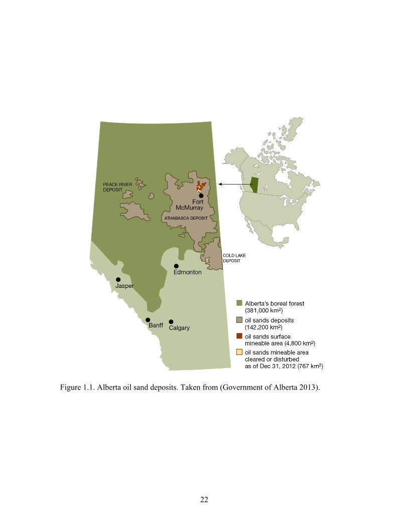
approximately 141,000 km2 (Masliyah et al. 2004). Figure 1.1 displays Alberta’s oil sand

deposits. Collectively Alberta’s oil sand deposits hold a remaining estimated established

reserve of about 20 x 109 m3 (Alberta Energy Resources 2012). However, Alberta oil

sands are estimated to hold some 200 x 109 m3 to 300 x 109 m3 of crude bitumen in total

(Kasperski and Mikula 2011, Morgan 2001). A significant portion, about 10%, of the

Athabasca oil sand deposit is located within the top 45 meters of the subsurface where

open pit mining is the most economically viable extraction method (Berkowitz and

Speight 1975). This portion of surface mineable oil sands is located in the northeast

2

portion of the Athabasca deposit centered on the town of Fort McMurray, Alberta, and

contains approximately 4 x 109 m3 of remaining established reserves of crude bitumen

(Alberta’s Energy Industry 2012). Open pit mining techniques result in large volumes of

waste, referred to as tailings, which require long term storage in structures known as

tailings ponds.

The oil sands operation, as a whole, consists of mining, extraction, upgrading

operations, and waste management. Proper integration of these four operations is

necessary for economically efficient bitumen recovery and for minimizing adverse

environmental impact (Masliyah et al. 2004). Without delving into too much detail, the

integrated open pit operation is as follows. Mined oil sand lumps are crushed and mixed

with heated recycled process water. Current operation slurry temperatures range between

40 to 55 ºC (Masliyah et al. 2004). This oil sand and water slurry is then directed to

hydrotransport pipelines or tumblers, where the oil sand lumps are sheared and lump size

is reduced. While in the hydrotransport pipelines or tumblers, the oil sand slurry is

treated with chemical additives to assist in bitumen liberation. The addition of sodium,

namely in the form of sodium hydroxide (NaOH), has been shown to increase bitumen

recovery rates (Sanford 1983). Air attaches to bitumen within the hydrotransport pipeline

or tumbler causing bitumen to float to the surface. The aerated bitumen is then skimmed

off the process slurry after reaching large gravity separation vessels. The subsequent

bitumen froth normally contains about 60% bitumen, 30% water, and 10% solids. This

froth is then diluted with a solvent which facilitates the removal of solids and water

within a settling vessel. Bitumen which was not captured in the initial aeration and

3

settling process is recovered in small amounts separately in secondary process streams.

Bitumen recovery rate is usually about 88 to 95% (Masliyah et al. 2004).

The remaining water and solids from both the initial slurry and the froth, referred

to as tailings, are directed to tailings ponds for storage, treatment, and water/solids

separation. Tailings which enter the pond are a mixture of about 55wt% solids, of which

82wt% is sand, 17wt% are fines smaller than 44 µm and 1wt% bitumen (Chalaturnyk et

al. 2002, Kasperski and Mikula 2011). The tailings usually have elevated salinity from

both natural and artificial sources in the bitumen extraction process. Salinity generally

increases as process water is continually recycled (Renault et al 1998). Tailings dam

dykes are constructed gradually, utilizing the coarser fraction (although still relatively

fine for sand) of beached tailings which settles from the initial tailings slurry, to support

ever increasing volumes of tailings. The underlying goal is that, following the closure of

the oil sands operation, the site will be reclaimed. Geotechnical and environmental

concerns present a need for effective and efficient monitoring techniques. The integrated

geophysical characterization, presented in this study, provides insight into the

applicability of geophysical methods towards geotechnical and environmental

monitoring.

1.2 Study Site: Syncrude’s Southwest Sand Storage Facility

The Syncrude Canada Ltd. Southwest Sand Storage Facility (SWSS) is located in

the southwest corner of the Mildred Lake Oil Sands Mine, approximately 35 kilometers

northwest of Fort McMurray, Alberta. The SWSS is a large tailings pond, covering an

area of approximately 25 km2, with the dyke measuring about 40 m high and up to 1 km

wide. The dyke is referred to as undrained in this report because there is was artificial

4

drainage system internally during the time in which data was collected for this study. It

contains nearly 300 million cubic meters of tailings (Price 2005). The facility was

commissioned in 1991 with three coarse tailing systems and a fluid return system,

providing coarse tailings sand storage and a small operating pond. The fluid return

system returned water and fluid fine tailings from the SWSS operating pond to the

Mildred Lake Settling Basin, a Syncrude operated tailings pond to the northeast of the

SWSS (Syncrude 2010). Between its commission and 2009, the dyke was constructed

using the upstream method. This method builds subsequent dykes upstream, towards the

tailings pond, from the initial starter dyke (Hoare 1972). Following dyke construction,

about an 80 cm thick layer of reclamation material was placed on the outside of the dyke,

consisting of peat and clay till mixture (Naeth et al 2011). However, the SWSS presented

reclamation challenges due to high water tables which resulted in process affected water

seeping into reclamation materials (Naeth et al. 2011). In 2009, it was redesigned to

support increase volumes of mature fine tailings (MFT) and fluid capacity. This design

change required a shift to the centerline dyke construction method (Syncrude 2008). This

method builds subsequent dykes which maintain the centerline of the starter dyke (Hoare

1972).

Figure 1.2 displays the general location and satellite image of the SWSS facility

in Alberta. The SWSS dyke was constructed with a terraced slope including benches

(backslopes). The portion of the dyke within the study area consists of four slopes and

three benches, which collect and transfer water to a swale south of the study area. Slopes

are in this area are 100 to 120 m wide and graded to 8 to 9%; benches are 70 to 90 m

5

wide and graded to approximately 1%. At the toe of the dyke a perimeter ditch collects

runoff and groundwater discharge.

1.3 Parameters of Interest and Petrophysical Model

Efficient geotechnical and environmental monitoring of tailings sites is important

to ensure dam safety and improve reclamation efforts. Such monitoring can be assisted by

characterizing soil-moisture, water level, and salt distributions. Such a study was

conducted previously at the SWSS facility using traditional hydrogeological sampling

methods involving many well and piezometer installations (Price 2005). Following the

hydrogeological characterization, Price took the study further by implementing a

groundwater flow and transport model. In this study, hydrogeological data from Price and

coincidental geophysical data was integrated to not only further characterize soil-

moisture and salt distributions at the SWSS, but also explore the usefulness of

geophysical surveying as a characterization method. Geophysical methods inherently

provide a larger spatial extent, as well as being less expensive and relatively non-

intrusive compared to traditional hydrogeological methods. However, the drawback of

geophysical surveying is that petrophysical model and relationships must be constructed

to convert geophysical parameters, collected through surveying, to desired parameters of

interest, e.g. soil-moisture and salinity.

The geophysical methods used in this study provide estimates for bulk electrical

conductivity (EC). To convert bulk EC measurements to parameters of interest, a

petrophysical model is required. In 1942, Gus Archie empirically developed a model

which relates bulk EC, fluid EC, and saturation within a porous medium (Archie 1942).

This model has since become known as Archie’s Law, equation 1.

6

where, (1)

and σb is bulk EC, sw is water saturation, n is the saturation exponent, σw is fluid EC, φ is

porosity, m is the cement factor, and a is the tortuosity factor. This expression is only

applicable in cases of clean or clay-free materials. When clay minerals are present, the

exchange of cations from the clay mineral surface with the pore electrolyte must be

considered (Devarajan 2006). The behavior of these exchange cations within an electrical

field has been described by an empirically derived model presented by Waxman and

Smits (1968). Another interpretation is that these hydrated cations form a “double layer”

close to the grain surface. This led to the development of Dual-Water (DW) empirical

model describing the electrical behavior of a porous medium which contains clay

minerals, presented by Clavier et al. (1984). These two models for shaly sands (clay

minerals present) are the most commonly used, however many more exist. Furthermore,

temperature has been shown to have a strong influence on EC (Waxman and Thomas

1974, Sen and Goode 1992).

In the case of the SWSS facility however, petrophysical models of shaly sands

can be ignored due to the low clay content of the tailings material which forms the dyke.

This leaves Archie’s law as a suitable petrophysical model to interpret bulk EC

measurements from geophysical surveying. Unfortunately, limited subsurface

temperature data were recorded during this study and the complex temperature

distribution could not be adequately modeled. The effects of temperature on bulk EC

were therefore left unaccounted for. This inhibits the quantitative capabilities of this

study, however many valuable qualitative interpretations can still be made, as well as

empirical estimates for parameters within the Archie law petrophysical model.

7

1.4 Geophysical Methods

1.4.1 Push Tool Conductivity

Push tool conductivity (PTC), also called direct-push conductivity, is an electrical

logging based method in which an EC probe is driven directly into the subsurface,

usually by a small truck-mounted rig or hydraulic hammer. The EC probe used in the

PTC method consists of four electrodes or contact rings in a set array with known

geometry. Figure 1.3 displays a schematic of a typical PTC probe and a photograph of the

rig used in this study. This design is similar to other electrical geophysical methods in

that an apparent resistivity (and its inverse, conductivity) is calculated by applying a

geometric factor to the ratio of measured induced potential to a known injected current. A

variety of electrode array types are used on current EC probes; most commonly the

Wenner array, but also Schlumbeger and Dipole-dipole arrays have been utilized (Beck

2000, Christy 1994, Schulmeister 2003). Figure 1.4 shows a schematic of common

electrode arrays, as well as their respective geometric factors used to calculate apparent

resistivity. The probe is usually advanced in small increments; for this study, a

conductivity measurement was taken every 1.64 cm. This provides a high resolution EC

profile of the subsurface. PTC probes also allow direct contact with subsurface materials,

while the accuracy of traditional borehole based EC logging methods may be negatively

influenced by irregular borehole diameter and drilling fluids (Shulmeister 2003). PTC

data are often assumed to be the most accurate representation of subsurface conductivity,

making it useful for comparison with other less direct geophysical techniques (Bentley

and Gharibi 2004, Hayley et al. 2009).

There are, however, some limitations to the method. First, the probe requires

careful calibration to prevent error in the measured EC. This is typically done by using a

8

factory supplied series of resistors and should be performed prior to each log test.

Secondly, the measured EC may be affected by the rate of advancement of the tool,

where negative and positive spikes in the measured EC may be a result of decrease or

increase of the rate of advancement respectively (Harrinton and Hendry 2006). In

addition, physical limitations exist where large rocks or heavily consolidated layers may

halt the advancement of the PTC probe.

1.4.2 Electromagnetic Surveying

Electromagnetic (EM) surveying techniques include a broad range of data

acquisition instruments and applications. In general, EM geophysical techniques refer to

methods which record the EM response of the subsurface to either an artificially or

naturally produced EM field. In active EM methods, a transmitter coil is used to generate

an EM field, referred to as the primary EM field. If a conductive medium is present in the

subsurface, the magnetic component of the incident EM wave induces eddy currents.

Eddy currents generate their own secondary EM field which can be detected by a

receiver. The secondary EM field will differ in both phase and amplitude to the known

primary field. The degree in which these components differ reveals information about the

electrical properties of the subsurface (Reynolds 2011).

In this study, EM surveying will be used to refer to ground conductivity surveying

from dual-coil instrument, Geonics EM-38. This instrument contains two separate coils;

one serves as a transmitter which generates the primary EM field, and one acts as a

receiver. The inter-coil spacing is fixed at one meter for the EM-38 device, and the dual-

coil system is moved along a study transect. The device records both quadrature and in-

phase components of the secondary EM field. The quadrature component can be directly

9

translated to an apparent conductivity, which is reported in milli-Siemens per meter

(mS/m). The in-phase component is measured in parts per thousand (ppt) and provides an

estimate for soil magnetic susceptibility. To rapidly collect data across the SWSS site, the

EM-38 was placed in a small plastic sled and connected to an all-terrain vehicle (ATV).

Figure 1.5 contains photographs of the EM-38 device and the EM-38 survey via ATV.

Ground conductivity meters respond to the conductivity composition of the

subsurface depending on the inter-coil spacing and magnetic dipole orientation.

Typically, as is the case for the EM-38 instrument, there are two modes in which data can

be collected; vertical magnetic dipole and horizontal magnetic dipole. The dipole

orientations have different response functions, i.e. contribution to apparent conductivity

with depth. Figure 1.6 displays the response functions or relative sensitivity with depth

for the EM-38 for both vertical and horizontal dipole orientations. In the case of the

vertical magnetic dipole, there is less contribution to measured apparent conductivity

from the near subsurface than in the horizontal dipole configuration. The maximum

response occurs below the near subsurface, depending on inter-coil separation. For the

EM-38, this depth is about 0.4 meters. For the horizontal magnetic dipole, the maximum

contribution or sensitivity occurs at the surface and decreases with increasing subsurface

depth. Consequently, the horizontal dipole orientation is very sensitive to near

subsurface changes in conductivity, while the vertical dipole orientation is less so. The

total secondary EM field, translated to apparent conductivity and measured at the receiver

coil, is the integral of the respective response function from zero to infinity, assuming a

homogenous subsurface half space (McNeill 1980).

10

1.4.3 Electrical Resistivity Tomography

Electrical resistivity tomography (ERT) is a geophysical technique which images

subsurface features from electrical resistivity measurements made at the surface and/or

within boreholes. Generally in field electrical resistivity (ER) methods, a current is

applied to the subsurface using two electrodes and the potential (voltage) is measured

between two separate electrodes. By combining Ohm’s Law with known electrode

geometry, the ER of the subsurface can be calculated, assuming a homogenous and

isotropic half-space. Realistically, the subsurface may consist of many electrically

different layers or features, and thus the calculated resistivity is not a ‘true’ resistivity, but

rather an apparent resistivity (Reynolds 2011). Distinct electrode arrays with known

geometries were developed, such as Wenner, Schlumberger, or dipole-dipole arrays

(Figure 1.4), which provided varying sensitivity to subsurface resistivity features. More

recently, computerized inverse modeling techniques allow for irregular array geometries

and data acquisition. However, classic array surveys are still frequently conducted by

convention.

In two-dimensional ERT methods, strings of electrodes are laid out in a line and

apparent ER data are collected automatically, controlled from a laptop or ER system,

using a pre-defined sequence of electrode sampling locations. In the automated data

acquisition sequence, sets of four electrodes (quadrupoles) are selected for the application

of current and measuring of potential. Many positions and electrode geometries are

sampled, including reciprocal measurements, as defined by the user. Resistivity

information can be found at increasing depths by increasing electrode separation within

the quadrupoles, at a cost of resolution (Reynolds 2011). Current ER systems typically

consist of 72 (or more) channels, allowing for 72 separate electrode positions to be

11

sampled in one continuous survey. The ER system used in this study was the ABEM

Terrameter SAS 300C (Figure 1.7). If a survey requires a longer study transect, the entire

72 electrode array is shifted, and the automated data acquisition software is run again.

Once the entire survey has been completed, all sampled electrode positions and measured

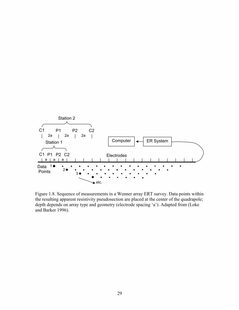
apparent resistivities may be combined to generate one image or pseudosection. Figure

1.8 shows a schematic of the ERT methodology using the Wenner array, and includes

data point locations which would be used to develop the resulting pseudosection of

apparent resistivity. These pseudosections yield a representation of subsurface resistivity.

However they are highly dependent on not only true subsurface resistivity distribution,

but also the electrode geometry and data acquisition sequencing (Loke and Barker 1996).

Currently, in nearly all levels of academic and commercial ERT surveys, inverse

modeling techniques are applied to generate models of the subsurface resistivity

distribution.

Given a resistivity model of the subsurface and the physics of the ER problem, it

is possible to calculate a set of apparent resistivity values which would be observed by an

ERT survey, under specific acquisition geometry and array sequencing. This process is

called forward modeling. Using an iterative least-squares approach, it is possible to find a

parameterized model space of resistivity which minimizes the difference between

forward-modeled resistances and observed resistances. In this study, RES2DINV was

used, an inversion software based on a smoothness-constrained, least-squares inversion

method (Loke and Barker 1996). Most often, the model space is overparameterized (more

parameters than data) and needs regularization; a variety of regularizing techniques have

been created under physical, mathematical, and empirical inspirations (Ellis and

12

Oldenburg 1994). Some examples of regularization schemes include classical Marquardt

(1970), Tikhonov (1977), and truncated singular value decomposition (TSVD) which is

outlined in Hansen (1987), as well as more recent methods including an Occam’s razor

approach which yields the most simple and smoothest model to prevent over-

interpretation by the practitioner (Constable et al. 1987). ERT inversions are affected by

both the sensitivity of the method and the effects of regularization. Final inverted

tomograms or models are dependent on the true distribution of subsurface resistivity,

method and quality of data acquisition, model parameterization, and the constraint

criteria (Singha and Gorelick 2006). Consequently, the solution to the problem is non-

unique and may contain artifacts, as well as a smoothed representation of subsurface

features.

The question remains however, in what way can we deal with the non-uniqueness

of the inverse problem, i.e., how do we know which model produced through inversion

procedures best represents the true earth? Many approaches have been taken to this

problem including a priori knowledge provided by geological or geotechnical surveys

(Ellis and Oldenburg 1994, Yeh et al. 2002), characterizing an error model to weight

measured data (Binley et al. 1995, Singha and Gorelick 2006), and matching inverse

models to supplementary data (Hayley et al 2009). In this study the latter approach was

taken, where final inverse models were chosen based on best agreement with coincidental

PTC data. The limitation of this particular method is that relationships between inverted

models and supplementary data may still be subject to variable model resolution and

regularization criteria in the inversion, as discussed previously. Nonetheless, it provides a

13

reasonable method for determining which inverted model should be chosen which best

represents the true resistivity distribution of the subsurface.

1.5 Hydrogeological Methods

1.5.1 Neutron Probe and Soil Moisture

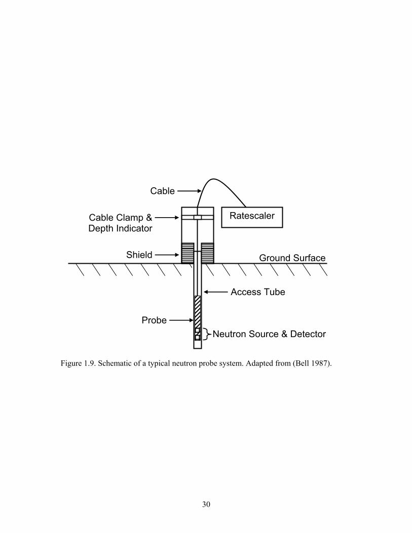
The neutron soil moisture gauge, commonly referred to as the neutron probe, is

designed to provide estimates of soil moisture. The device basically consists of a fast

neutron source, a slow neutron detector, a pulse counter (ratescaler), a cable connecting

the two, and a transport shield (Bell 1987). For most systems, the transport shield is fitted

to a vertical aluminum access tube which slightly protrudes from the subsurface.

Following, the probe is lowered from the transport shield through the access tube,

recording successive measurements with depth to create a profile. The transport shield

generally consists of a plastic neutron moderator which provides shielding from the fast

neutron source (Bell 1987). The ratescaler remains at the surface. Figure 1.9 displays a

schematic of a typical neutron probe.

The probe contains a radioactive source which emits fast neutrons into the

surrounding subsurface. When the emitted fast neutrons collide with the nuclei of other

atoms, predominately hydrogen nuclei, the neutrons scatter, slow down, and lose energy.

It should be noted that although hydrogen nuclei, including bound water and organic

materials, exerts the primary effect on the count rate, every element has some ability to

scatter and slow fast neutrons (Bell 1987). This creates a ‘cloud’ of slow neutrons around

the neutron source and the density of this cloud, which is mainly a function of soil

moisture, is sampled through the detector. The mean count rate is subsequently displayed

on the ratescaler and can be translated to soil moisture, namely volumetric moisture,

14

using an appropriate calibration curve. Count rates are usually expressed as a count ratio,

the number of counts at a given depth relative to the counts in a standard moderator to

eliminate error due to instrument drift (Vachaud 1977). The generation of specific field

calibration curves is necessary to ensure accurate results, however calibration methods

are difficult to perform and regression correlation coefficients between count ratio and

soil moisture content are not extremely high, usually between 0.80 and 0.95 (Reichardt

1997, Vachaud et al 1977). Despite the difficulties in the calibration of neutron probes,

they have been successfully employed in a variety of studies (Grant et al. 2004, Huo et al.

2008, Evett et al. 2009, Hu et al. 2009).

1.5.2 Groundwater Sampling

Traditional groundwater sampling techniques include the drilling of boreholes and

the installation of wells or piezometers. Both the well size, in diameter, and the length of

the well screen, the slotted area in which water can flow into the well, depends on the

application. Small well diameters, given they are large enough for sampling equipment

and probes, are preferred in groundwater sampling applications because they are less

expensive, easier to install, and are smaller in volume. Large screen lengths will provide

non-depth specific groundwater samples that are integrated over the length of the screen,

with high permeability units contributing more water than low permeability units.

Generally however, in groundwater sampling applications where detailed groundwater

characterization is necessary, small screen lengths are utilized as they provide depth

specific information (Appelo and Postma 2005). To acquire depth specific sampling at

multiple depths, multi-level wells or piezometer nests are required. This study, and the

previous hydrogeological characterization of the SWSS site conducted by Price (Price

15

2005), utilized a series of piezometer nests where each piezometer is placed in separate

boreholes and clustered in close proximity to one another.

Drilling operations, including drilling fluids, gravel packs, or casing materials,

often disturb the natural chemistry and flow conditions of a well. To return groundwater

produced by the well to its natural conditions, the well is flushed by drawing water from

the well until the parameters of interest stabilize. This may vary between 2 to 10 well

volumes depending on the local hydrological conditions (Appelo and Postma 2005).

Once well or piezometer installation and flushing is completed, water samples are

acquired and measured for a variety of parameters, in both the field and laboratory.

To acquire water level information well screens must be placed solely in the

desired unit, as different units may be of varying hydraulic potential and result in

inaccurate water level measurements (Appelo and Postma 2005). In the case of the SWSS

site, the tailings material which forms the dyke represents the uppermost aquifer and the

unit of interest. Thus water level wells were installed with screened intervals across the

water table within the tailings dyke. Furthermore, a large number of piezometer nests at

varying depths were installed during for the groundwater sampling program.

1.6 Purpose and Scope

With the growing number of tailings sites as a result of surface mined oil sands,

there is a need to develop methods to efficiently monitor soil moisture and salt transport

for both geotechnical and environmental concerns. A previous groundwater modeling

study at the SWSS facility evaluated flow and salt transport, calibrated with

hydrogeological field data, under varying hydrological inputs, boundary condition, and

physical properties (Price 2005). The research presented in this study, aimed to improve

16

the understanding of flow and salt transport within the SWSS dyke and other tailings dam

structures by augmenting hydrogeological data with geophysical data. Overall, this work

helps improve tailings site monitoring methods and facilitates future geotechnical and

environmental management of the SWSS site and other tailings sites. The research

presents benefits and limitations of using geophysical methods to monitor tailings sand

dykes. Furthermore, the applicability of geophysical data to aid in the calibration and

validation of future groundwater flow models were investigated.

1.7 Study Objectives

In this study, the applicability of combined geophysical methods and

hydrogeological measurements to map and monitor soil moisture and salt distribution at

oil sands tailings sites is investigated. Furthermore, the usefulness of geophysical

methods to the calibration and validation of groundwater flow and transport models is

explored. This was achieved by developing a geophysical characterization of the SWSS

site, using both forward and inverse modeling techniques to aid in the calibration and

imaging of site bulk electrical conductivity. Furthermore, the petrophysical relationships

between geophysical and hydrogeological data were investigated; specifically the

relationships between bulk electrical conductivity versus soil moisture and fluid electrical

conductivity were explored.

1.8 Contribution of Authors

Chapter 2 of this thesis is presented as a stand-alone manuscript.

Booterbaugh, A.P, Bentley, L.R., Mendoza, C.A. (in prep.). Geophysical characterization of an undrained oil sands tailings pond Alberta, Canada. JEEG.

17

Geophysical data were collected by Komex International Ltd. in 2001 and 2004,

and WorleyParsons Ltd. in 2008. Hydrogeological data were collected by C.A.M. at the

University of Alberta. A.P.B. processed all of the geophysical and hydrogeological data

used in this study. Additionally, A.P.B developed and utilized MATLAB codes

contained in the Appendix section; A.P.B. developed the method for normalizing the EM

maps and automated layer designation for PTC data. The interpretations of results were

made by A.P.B. following extensive discussions with L.R.B. and C.A.M.. A.P.B. wrote

the manuscript.

18

1.9 References

Alberta’s Energy Industry. An Overview. 2012. Alberta Energy Resources Conservation Board.

Appelo, C. and Postma, D. 2005. Geochemistry, groundwater and pollution. 2nd Edition.

A.A. Balkema Publishers, Leiden, The Netherlands a member of Taylor & Fancis Group plc.

Archie, G. 1942. The electrical resistivity log as an aid in determining some reservoir

characteristics. T. Am. I. Min. Met. Eng., Vol. 146. 54 – 62. Beck, F., Clark, P., Puls, R. 2000. Location and characterization of subsurface anomalies

using a soil conductivity probe. Bell, J. 1987. Neutron probe practice. 3rd edition. Inst. of Hydrol., Rep. 19. 1 – 63. Bentley, L., Gharibi, M. 2004. Two- and three-dimensional electrical resistivity imaging

at a heterogeneous remediation site. Geophysics. Vol. 69, No. 3. 674 – 680. Berkowitz, N. and Speight, J. 1975. The oil sands of Alberta. Fuel. Vol. 54. 138 – 149. Binley, A., Ramirez, A., Daily, W. 1995. Regularised image reconstruction on noisy

electrical resistance tomography data: 4th Workshop of the European Concerted Action on Process Tomography, Proceedings. 401 – 410.

Clavier, C., Coates, G., Dumanoir, J. 1984. Theoretical and experimental bases for the

Dual-Water model for interpretation of shaly sands. Soc Petrol Eng J. Vol. 24. No. 2. 153 – 168.

Chirsty, C., Christy, T., Witting, V. 1994. A percussion probing tool for direct sensing of

soil conductivity. Proceedings of the 8th National Outdoor Action Conference. 381 – 394.

Constable, S., Parker, R., Constable, C. 1987. Occam’s inversion: a practical algorithm

for generating smooth models from EM sounding data. Geophysics. Vol. 52. 289 – 300.

Devarajan, S., Toumelin, E., Torres-Verdin, C. 2006. Pore-scale analysis of the Waxman-

Smits shaly sand conductivity model. SPWLA 47th Annual Logging Symposium, Vera Cruz, Mexico. 1- 9.

Ellis, R. and Oldenburg, D. 1994. Applied geophysical inversion. Geophys. J. Int. Vol.

116. 5 – 11.

19

Evett, S., Schwartz, R., Tolk, J., Howell, T. 2009. Soil profile water content determination: Spatiotemporal variability of electromagnetic and neutron probe sensors in access tubes. Vadose Zone J. Vol. 8. 926 – 941.

Government of Alberta. 2013. Oil Sands Reclamation.

www.oilsands.alberta.ca/reclamation. html. Grant, L., Seyfried, M., McNamara, J. 2004. Spatial variation and temporal stability of

soil water in a snow-dominated mountain catchment. Hydrol. Process. Vol. 18. 3493 – 3511.

Hansen, C. 1987. The truncated SVD as a method for regularization. BIT. Vol. 27. No. 4.

534 – 553. Harrinton, G. and Hendry, M. 2006. Using direct-push EC logging to delineate

heterogeneity in a clay-rich aquitard. Ground Water Monit. Rem. Vol. 26. No. 1. 92 – 100.

Hayley, K., Bentley, L., Gharibi, M. 2009. Time-lapse electrical resistivity monitoring of

salt-affected soil and groundwater. Water. Resour. Res. Vol. 45. 1 – 14. Hoare, B. 1972. The disposal of mine tailings material. (Doctoral dissertation). University

of Waterloo. 1-210. Hu, W., Shao, M., Wang, Q., Reichardt, K. 2009. Time stability of soil water storage

measured by neutron probe and the effects of calibration procedures in a small watershed. Catena. Vol. 79. 72 – 82.

Huo, Z., Shao, M., Horton, R. 2008. Impact of gully on soil moisture of shrubland in

wind-water erosion crisscross region of the Loess Plateau. Pedosphere. Vol. 18. No. 5. 674 – 680.

Komex International Ltd. 2001. C55100000: Geophysical characterization of the

Southwest Sand Storage Facility. Syncrude Canada Ltd., Fort McMurray, Alberta. Komex International Ltd. 2005. E00050405: 2004 Geophysical Investigation of

Southwest Sand Storage Facility. Syncrude Canada Ltd., Fort McMurray, Alberta. Loke, M., and Barker, R. 1996. Rapid least-squares inversion of apparent resistivity

pseudosections by a quasi-Newton method. Geophys. Prospect. Vol. 44. 131-152. Marquardt, D. 1970. Generalized inverses, ridge regression, biased linear estimation, and

nonlinear estimation. Technometrics. Vol. 12. 591 – 612.

20

Masliyah, J., Zhou, Z., Xu, Z., Czarnecki, J., Hamza, H. 2004. Understanding water-based bitumen extraction from Athabasca Oil Sands. Can. J. Chem. Eng. Vol. 82. 628 – 654.

Morgan, G. 2001. An energy renaissance in oil sands development. World Energy. Vol.4,

No. 2. 46 – 53. McNeill, J. 1980. Electromagnetic terrain conductivity measurement at low induction

numbers. Technical Note TN-6, Geonics Ltd., Mississauga, Ontario, Canada. Naeth, M., Chanasyk, D., Burgers, T. 2011. Vegetation and soil water interactions on a

tailings sand storage facility in the Athabasca oil sands region of Alberta Canada. Phys. Chem. Earth. Vol. 36. 19-30.

Price, A. 2005. Evaluation of groundwater flow and salt transport within an undrained

tailings sand dam (Master’s Thesis). University of Alberta, Department of Earth and Atmospheric Sciences.

Reichardt, K., Portezan, O., Bacchi, O., Oliveira, J., Douradoneto, D., Pilotto, J., Calvache, M. 1997. Neutron probe calibration correction by temporal stability parameters of soil water content probability distribution. Sci. Agric. Vol. 54. 17 – 21.

Renault, S., Lait, C., Zwiazek, J., MacKinnon, M. 1998. Effect of high salinity tailings

waters produced from gypsum treatment of oil sands tailings on plants of the boreal forest. Environ. Pollut. Vol. 102. 177 – 184.

Reynolds, J. 2011. An introduction to applied and environmental geophysics – 2nd ed.

Wiley – Blackwell. Chichester, UK. Sanford, E. 1983. Processibility of Athabasca oil sand: Interrelationship between oil sand

fine solids, process aids, mechanical energy and oil sand age after mining. Can. J. Chem. Eng. Vol 61. 554 – 567.

Sen, P. and Goode, P. 1992. Influence of temperature on electrical conductivity on shaly

sands. Geophysics. Vol. 57. No. 1. 89 – 96. Singha, K., Gorelick, S. 2006. Effects of spatially variable resolution on field-scale

estimates of tracer concentration from electrical inversions using Archies’s law. Geophysics. Vol. 71, No. 3. G83 – G91.

Schulmeister, M., Butler, J., Healey, J., Zheng, L., Wysocki, D., McCall, G. 2003. Direct-

push electrical conductivity logging for high-resolution hydrostratigraphic characterization. Ground Water Monit. Rem. Vol. 23, No. 3. 52 – 62.

21

Syncrude Canada Ltd.. 2008. Public Disclosure Document: South west sand storage Conversion. Phys. Chem. Earth. Vol. 36. 19 – 30.

Syncrude Canada Ltd. 2010. Directive 074: Baseline Survey for Fluid Deposits Syncrude Mildred Lake and Aurora North. Alberta Energy Resources. 1 – 49.

Tikhonov, A. and Valette, B. 1977. Solutions of ill-posed problems. John-Wiley & Sons,

New York. Vachaud, G., Royer, J., Cooper, J. 1977. Comparison of methods of calibration of a

neutron probe by gravimetry or neutron-capture model. J. Hydrol. Vol. 34. 343 – 356.

Waxman, M. and Smits, L. 1968. Electrical conductivities in oil-bearing shaly sands. Soc

Petrol Eng J. Vol. 8. 107 – 122. Waxman, M. and Thomas, E. Elecrical conductivities in shaly sands- I. The relation

between hydrocarbon saturation and resistivity index; II. The temperature coefficient of electrical conductivity. J. Petrol. Technol. Vol. 26. No. 2. 213 – 225.

Yeh, T., Liu, S., Glass, R., Barker, K., Brainard, J., Alumbaugh, D., LaBrecque, D. 2002.

A geostatistically based inverse model for electrical resistivbity surveys and its applications to vadose zone hydrology. Water Resour. Res. Vol. 38. No. 12. 1 – 13.

22

Figure 1.1. Alberta oil sand deposits. Taken from (Government of Alberta 2013).

23

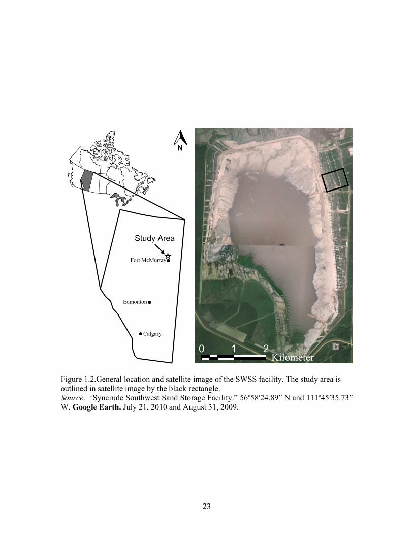
Figure 1.2.General location and satellite image of the SWSS facility. The study area is outlined in satellite image by the black rectangle. Source: “Syncrude Southwest Sand Storage Facility.” 56º58′24.89′′ N and 111º45′35.73′′ W. Google Earth. July 21, 2010 and August 31, 2009.

Kilometer 0 1 2

Study Area

Edmonton

Calgary

Fort McMurray

24

Figure 1.3. Schematic of PTC probe (left) and photograph of truck mounted rig for PTC implementation (right) at the SWSS facility. Schematic adapted from (Schulmeister 2003). Photograph from (Komex 2001).

Electrode Array

25

Figure 1.4. Common electrode arrays and geometric factors utilized in EC probes, as well as ER surveys. Adapted from (Reynolds 2011).

P2

C2

ρa = 2πa(V/I) 

ρa = πn(n+1)(n+2)a(V/I)

a a

b

a 

a

P1 P2 C2

P1

C1

C2 C1

P1 P2 C1

Wenner 

Schlumberger 

Dipole‐dipole 

ρa = (πa2/b)[1‐(b2/4a2)](V/I)

a 

naa 

a

26

Figure 1.5. Photograph of the EM-38 device (top right) and photographs of EM-38 surveying with use of an ATV, conducted at the SWSS facility (Komex 2001).

27

Figure 1.6. Response functions for EM-38 device for both vertical and horizontal dipole orientations. Adapted from (McNeill 1980).

28

Figure 1.7. Photograph of the ERT system used in this study, the ABEM Terrameter 300C (Komex 2005).

29

Figure 1.8. Sequence of measurements in a Wenner array ERT survey. Data points within the resulting apparent resistivity pseudosection are placed at the center of the quadrapole; depth depends on array type and geometry (electrode spacing ‘a’). Adapted from (Loke and Barker 1996).

C1 P1 P2 C2

Station 1

a a a

ER System Computer

C1 P1 P2 C2

Station 2

2a 2a 2a

Electrodes

etc.

1 2

3

Data Points

30

Figure 1.9. Schematic of a typical neutron probe system. Adapted from (Bell 1987).

Ground Surface

Access Tube

Cable

Neutron Source & Detector

Probe

Shield

Ratescaler Cable Clamp & Depth Indicator

31

Chapter 2: Geophysical characterization of an undrained dyke containing an oil-

sands tailings pond, Alberta, Canada

Abstract

Geophysical characterization of an undrained oil sands tailings pond dyke was

conducted at Syncrude Canada’s Southwest Sand Storage Facility (SWSS). Push tool

conductivity (PTC), electromagnetic (EM), and electrical resistivity tomography (ERT)

methods in tangent with hydrogeological and chemistry measurements were used to

investigate soil moisture, hydraulic heads, and groundwater salinity distributions.

Geophysical data were collected from 2001 to 2008 and interpretations can further be

used to validate studies of groundwater flow and salt transport within the structure. An

Archie’s Law petrophysical model was utilized to relate measured bulk conductivity,

from geophysical surveying, with measures of soil moisture and fluid electrical

conductivity. It was found that a relatively strong relationship between bulk electrical

conductivity and soil moisture exists, while weak to no correlation was observed between

bulk and fluid electrical conductivity. ERT surveying was capable of clearly identifying

the location of the water table within the dyke. This study provides a unique look into the

application of geophysical techniques to investigate soil moisture, hydraulic head, and

salt distribution in an active undrained tailings dam structure. The methodology and

insights gained from this study may be applied to similar undrained and drained oil sands

tailings storage sites.

2.1 Introduction

The processing and production of the Athabasca Oil Sand deposit in northern

Alberta, Canada has, in recent decades, grown into a large industry, producing about 2.3

32

x 105 m3 per day and expected to grow to 4.5 x 105 m3 per day by 2022 (Alberta Energy

Resources 2012). The Athabasca is the largest of three major oil sand deposits in Alberta

and collectively Alberta’s oil sands constitute the world’s largest bitumen reserve,

containing an initial in-place resource of approximately 200 x 109 m3, with an estimated

established reserve of 20 x 109 barrels (Kasperski and Mikula 2011). About one tenth of

the Athabasca oil sands deposit lies within the upper 45 meters of the subsurface where

conventional open pit mining operations are most economically viable (Berkowitz and

Speight 1975). Open pit mining operations of these near surface oil sand deposits results

in large volumes of waste referred to as tailings. Bitumen is extracted using a water-based

extraction process, a developed method that is similar in concept to the hot water

extraction method first described by Clark (1929). This method involves a warm water

slurry, typically 40 - 55ºC, and chemical additives, most notably NaOH, to assist in

bitumen liberation (Masliyah et al. 2004).

Tailings are collectively made up of a combination of coarser-grained sediments,

dispersed fines, process affected sodium-rich water, and residual bitumen. This slurry

has about 55wt% solids, of which 82wt% is sand, 17wt% are fines smaller than 44 µm

and 1wt% bitumen (Chalaturnyk et al. 2002, Kasperski and Mikula 2011). Tailings are

directed to waste storage facilities referred to as tailings ponds (Dusseault and Scott,

1983). Tailings dam dykes are constructed gradually, utilizing the coarser fraction

(although still relatively fine for sand) of beached tailings which settles from the initial

tailings slurry, to support ever increasing volumes of tailings. The underlying goal is

that, following closure of the oil sands production operation, the tailings pond sites will

be reclaimed. However, there is often a need to investigate and monitor soil moisture and

33

salinity within tailings pond structures for both geotechnical and environmental concerns.

Traditional hydrogeological monitoring techniques typically involve the installation of

wells and only provide sparse point measurements. With the addition of geophysical

techniques, sites may be mapped and monitored in a much more spatially extensive,

rapid, and less expensive manner.

The bulk electrical conductivity (EC) of the subsurface is dependent on several

parameters including soil type, soil moisture, fluid EC, and temperature. A petrophysical

relationship for sand was described and empirically derived by Archie (1942) and has

since become commonly known as Archie’s Law. Tailings used for dyke construction

provide an opportunity to build Archie’s law relationships because of their relatively clay

free properties. With available direct measures of soil moisture and fluid EC, as well as

geophysical measures of bulk EC, site specific empirical relationships can be developed.

Archie’s Law and its use as a petrophysical model for this study is described in more

detail later. Similar environmental and geotechnical geophysical investigations at mine

tailings and other contaminated sites have been conducted in recent years (Hayley et al

2009, Martínez-Pagán et al 2009, Sjödahl et al 2005, Yuval and Oldenburg 1996).

In this study, the applicability of combined geophysical methods and

hydrogeological measurements to map and monitor soil moisture and salt distribution at

oil sands tailings sites is investigated. Furthermore, the usefulness of geophysical

methods to the calibration and validation of groundwater flow and transport models is

explored.

34

2.2 Study Site: Syncrude’s Southwest Sand Storage Facility

The Southwest Sand Storage Facility (SWSS) is a large tailings pond located

approximately 35 kilometers northwest of Fort McMurray, Alberta in the southwest

corner the Syncrude Canada Ltd. Mildred Lake Oil Sands Lease. The SWSS dyke is up to

40 m high and 1 km wide and is referred to as undrained because there is no artificial

drainage system internally. Figure 2.1 displays the approximate location and satellite

image of the SWSS site, as well as a shaded relief map which includes sampling locations

for a variety methods conducted in this study. It was commissioned in 1991 and designed

to provide coarse tailings sand storage. It is 25 km2 in area and approximately 40 m in

height (Price 2005). Prior to 2009 and during the data acquisition for this study, the

structure was without an internal drainage system and the dyke was constructed with the

upstream method. The upstream construction method adds subsequent dykes upstream,

towards the tailings pond, from the starter dyke (Hoare 1972). An approximately 80 cm

thick layer of reclamation material, a peat and clay till mixture, was added following the

placement of coarse tailings which form the dyke. However, the SWSS dyke presented

reclamation challenges due to shallow water tables which, in some locations, resulted in

process affected tailings water seeping to reclamation materials (Naeth et al. 2011).

The SWSS facility dyke was constructed with terraced slopes including benches

(backslopes) creating a groundwater flow system conceptually similar to the classic small

drainage basin flow under sinusoidal topography described by Tóth (1963). The study

area in the northeast portion of the SWSS dyke consists of four slopes and three benches.

As a result of high water tables and ponded water at the toes of slopes, benches began to

function as a method of collecting and transferring runoff and seepage water to a swale

south of the study area, eventually reaching a perimeter ditch at the toe of the dyke

35

(Naeth et al. 2011). Figure 2.2 displays a cross-section of the study area and conceptual

groundwater flow with groundwater discharge and recharge areas in local topographic

lows of the benches.

2.3 Petrophysical Model

The tailings sand which makes up the SWSS dyke is believed to be a relatively

clay free sand. For this reason, as described previously, Archie’s Law is a reasonable

choice for the foundation of petrophysical relationships described in this study. Archie’s

description of the bulk EC of clay free porous medium is:

where, (1)

where σb is bulk EC, sw is water saturation, n is the saturation exponent, σw is fluid EC, φ

is porosity, m is the cement factor, and a is the tortuosity factor. F is known as the

formation factor. In areas below the water table, where water saturation equals 1, cross-

plots of coincidental bulk and fluid EC measurements should produce an estimate for F as

the slope of linear regression with y-intercept equal to zero. This direct relationship and

results which pertain from this study will be discussed later.

Additionally, Archie’s Law can be transformed into a version which linearly

relates bulk EC to saturation. Rearranging equation 1 with a logarithmic transform yields:

(2)

2.4 Materials and Methods

2.4.1 Data Acquisition

Geophysical methods for this study included push tool electrical conductivity

(PTC), frequency domain electromagnetic (EM), and electrical resistivity tomography

(ERT). Data for the three methods were collected in 2001 and 2004, with ERT also being

36

collected in 2008. Data were collected by Komex International Ltd. in 2001 and 2004,

and WorleyParsons Ltd. in 2008. In 2001 data were acquired along study transects A and

B (Figure 2.1), with EM taken over an extensive area of the northeast section of the

SWSS dyke. In 2002, a total of sixty-seven piezometers and water table wells were

installed along transect C to characterize hydraulic head and salt distribution.

Hydrogeological and chemistry data collected during 2002 to 2003 were synthesized into

a numerical model in order to evaluate groundwater flow and salt transport within the

SWSS dyke (Price 2005). With the additional instrumentation along transect C,

geophysical methods were refocused to transects A and C in 2004 and 2008, with the

hypothesis that the integration of these data would provide a more spatially exhaustive

image of hydraulic heads and salt distribution within the SWSS dyke.

2.4.2 Hydrogeological and Chemistry Methods

Hydrogeological and chemistry measurements were taken along Transect C

between 2002 and 2008, including water level, fluid EC, fluid or porous medium

temperature, total dissolved solids, pH, dissolved oxygen, and major anion and cation

concentration measurements. Of most interest in this study were water level and fluid EC

measurements which can be correlated directly with geophysical data. Figure 2.1 displays

the locations of the various hydrogeological sampling used in this study. Water level

measurements were taken from water table wells installed with 1 to 1.5 m screens across

the water table. Piezometers, used for groundwater sampling, were installed with 0.3 m

screens from 1 m below the water table to up to 9 m deep and spaced vertically by 2 m.

Wells and piezometers were constructed of 0.025 m diameter PVC pipe with machine

37

slotted screens (0.5 mm) covered in filter cloth, and installed using either a 1 inch hand

auger or a 3.5 inch portable solid-stem auger drill (Price 2005).

Volumetric moisture (VM) profiles were also collected along Transect C between

2001 and 2012 in the same locations where wells were installed (Figure 2.1), using either

a model 501DR or 503DR Campbell Pacific Nuclear Corp. neutron probe. The probe

contains a fast radioactive neutron source and a slow neutron detector. Fast neutrons are

released from the source, which collide with nuclei of similar mass, predominantly

hydrogen, slowing or thermalizing the neutrons. A ‘cloud’ of slow neutrons are generated

within the soil near the source; the density of this cloud is sampled and translated to an

estimate of VM. Other elements and hydrogen not associated with water may also cause

some additional scattering of fast neutrons, however measurements are largely a function

of soil moisture (Bell 1987). Measurements were taken every 15 cm to a depth of about

1.5 to 3 meters.

2.4.3 Push Tool Conductivity

A total of thirty-seven and sixteen PTC profiles were recorded for 2001 and 2004,

respectively. Measurements were taken to approximately 5 meters below the surface

with a sampling resolution of 1.64 cm. For areas which were easily accessible, near the

crest of the dyke where vegetation was thin, a rig mounted hydraulic hammer was used to

advance the PTC probe. In areas near the toe of the dyke which had more dense

vegetation, the PTC probe was driven into the ground by hand using a 13.6 kg slide

hammer (Komex 2004). PTC provides a relatively quick acquisition, high resolution

vertical EC profile and was assumed, for this study, to be the most accurate

representation of subsurface bulk EC. For this reason, PTC data was used to calibrate

38

EM and optimize ERT inversion; calibration and optimization procedures will be

discussed in the following sections. A simple 5-point triangle smoothing filter was

applied to raw PTC data to dampen high spatial frequency noise.

To calibrate EM data, which provides one integrated EC measurement of the

subsurface, to PTC data, which provides bulk EC measurements with depth, PTC data

was forward modeled to a simulated EM response using EM modeling software FreqEM

(Loke 2006). This model is based off a 1-D layered earth, with a maximum of 8 layers,

and is capable of both inversion and forward modeling of EM response of desired dipole

orientation and geometry. It was therefore necessary to divide PTC profiles into distinct

layers for which an EM response could be calculated through FreqEM. To achieve this

with minimal bias over a large number of PTC profiles, a program was developed to

automatically locate a desired number of layers from 1-D data (Appendix H). The

program starts with a high number of layers and is primarily constrained by a layer

variance threshold which is gradually increased until the model reaches the desired

number of layers. Other constraints include a limit to minimum and maximum layer size

which can be systematically increased with depth, and the percent change in mean values

over a specified window size. This allowed the program to pick both more layers near

the surface, within depths of high contribution to EM response, and layer boundaries at

areas of high EC change. A user defined depth of investigation parameter also allowed

constraints to be loosened with depth to improve model stability. Once layers were

developed for the PTC profiles, the mean EC and thickness of the modeled PTC layers

were implemented into the FreqEM package and forward modeled to a calculated EM EC

39

response. Examples of PTC profiles and their respective modeled layers may be found in

Appendix A.

2.4.4 Electromagnetic Methods

Electromagnetic (EM) surveys were taken in the fall of 2001 and 2004. In 2001

surveys were taken over a large section in the northeast region of the SWSS dyke. In

2004 surveys were focused on only transects A and C. The Geonics EM-38 device was

utilized in both cases and is particularly useful as a reconnaissance tool which can

quickly map EC of the upper subsurface. In order to acquire data rapidly over a large

area, the EM device was placed in a small sled designed to be pulled by an all terrain

vehicle (ATV). In areas where vegetation, soil conditions, or instrumentation prevented

the use of the ATV, the EM surveys were continued on foot. EM surveys were

conducted with both horizontal and vertical dipole orientations allowing for nominal

depths of exploration of 0.75 and 1.5 meters respectively. Only the data acquired in the

vertical orientation are reported in this paper.

In both 2001 and 2004, EM surveys were conducted over several days under

different moisture conditions due to rain. Consequently, large portions of EM data

displayed differences in average EC, due to differences in average soil moisture on

different days (Figure 3A). The largest discrepancies in EC existed along the upper parts

of the bench and slopes where water tables are lower. Conversely at the toes of the slopes

where water tables are high, the precipitation did not cause a large change in soil

moisture and subsequently measured apparent EC. In order for the data to be used to

make inferences on soil moisture and salinity, it was necessary to normalize the data so

that the different spatial regions have similar statistical distributions of EC. A

40

normalization procedure was developed to shift the statistical distribution of measured

EC in elevated zones of EM data, to a distribution of EC that was similar to surrounding

EM data (Appendix G). A key component which made the normalization possible was

that the SWSS dyke is an engineered structure which contains linear topographic features

perpendicular to its aspect. Similarly, it was assumed that EC across the SWSS site

should reflect this linearity, i.e., the EC statistics should display stationarity in space

perpendicular to the dykes slope, given the same surface moisture conditions. Preliminary

EM maps of non-elevated EC regions confirmed this assumption.

First, two zones of EM data which should display similar statistical distributions

were selected; one of elevated EC and one of a reference EC. Data from the two zones

were broken into 100 quantiles (percentiles) and the difference between the mean of the

elevated data and the mean of the reference data at each respective quantile was

calculated. Following, a piecewise linear function was developed consecutively

connecting the calculated mean difference at each quantile. This created a continuous,

polygonal curve in which the difference between the elevated and reference region could

then be estimated for each data point in the elevated region. The data in the elevated

region were then adjusted by the appropriate estimated difference from the polygonal

curve, creating a normalized elevated region which statistically matched the reference

region. This was done in several iterations until elevated EC regions displayed similar EC

statistics to that of the non-elevated data region in space perpendicular to the dyke aspect.

Elevated zones were defined by selecting regions which exhibited elevated EM EC of

about 50 – 70 mS/m (uncalibrated conductivity) along the upper parts of the slopes and

benches. Reference zones were selected in areas that show display statistical stationarity

41

to elevated zones. Elevated and reference zones were also selected to contain areas

including the toes of the slopes where measured EC was high. As mentioned previously

there was little discrepancy in measured EC between the elevated and reference zones in

these areas due to already high water tables. Incorporating this high EC and statistically

stationary area in the normalization procedure allowed the higher EC values in the total

EC distribution to be well defined and provided a greater range of EC, which overall

improved the normalization procedure results. Figure 2.3 displays contoured data and

histograms for one normalization procedure of the 2001 EM data. Summary statistics for

the normalization example of Figure 2.3 can be found in Table 2.1. Sections in the

normalization example are labeled X, Y, & Z for comparison to histograms and summary

statistics.

Following normalization, it was possible to calibrate the EM data to the calculated

EM response from PTC data as discussed previously. The inverse distance interpolation

method was used to estimate EM EC at the location of each PTC survey for 2001 and

2004. The resulting collocated EM EC data and calculated EM EC data were cross-

plotted. A linear regression model with the y-intercept forced through zero was used to

calibrate raw EM data in both 2001 and 2004 (Figure 2.4).

2.4.5 Electrical Resistivity Tomography

Electrical resistivity tomography surveys were conducted on the SWSS dyke in

the fall of 2001, 2004 and 2008. Surveys were conducted using the Wenner array, one

meter electrode spacing with a maximum a-spacing of 24 meters, and a total length

varying from 600 to 800 meters. Data was inverted using finite difference resistivity

inversion package Res2Dinv (Loke and Barker 1996). Inversion parameters within

42

Res2Dinv were optimized manually by finding the highest correlation coefficient

between inverted ERT data and coincidental PTC data averaged across the inversion

mesh. The correlation coefficient, as opposed to the sum square error (SSE) as utilized in

Hayley et al. (2009), was deemed to be the strongest indicator of the best inverse model

because the relationship between ERT EC and PTC EC did not seem to follow a ‘1 to 1’

relationship, where error metrics would be most suitable. The cause of this may be a

result of temporal discrepancies in PTC and ERT surveying and/or PTC calibration.

Inversion parameters which had the greatest influence on the inversion results were data

and model norms, vertical to horizontal flatness filter, vertical dampening, and mesh

discretization. Table 2.2 outlines and provides values for these inversion parameters.

Many other inversion parameters were tested yet inversion results were largely

insensitive to parameters outside the ones listed.

Once inversion parameters were optimized, all ERT data were inverted under the

same parameters and cross-plotted with PTC for calibration in a similar fashion as with

EM methods. It should be noted that resistivity inversion techniques are fundamentally

ill-posed problems which provide non-unique answers. Subsequently, calibration plots

are subject to this non-uniqueness and should be considered as such. Confidence in

calibration models follows from correlation strength between inverted ERT data and PTC

data. However, due to smoothing of inverted ERT models, inversion procedures are often

incapable of resolving sharp boundaries which were typically observed in PTC data at the

SWSS. With regard to this, some scatter from the calibration model is expected and

overall does not detract from confidence in the calibration. Furthermore, sharp EC

contrasts were usually observed from low to high EC with depth, creating a scenario of

43

underestimating EC of ERT models in low ERT EC ranges. This can readily be observed

in calibration plots, especially for 2004. Figure 2.5 displays cross-plots and calibrations

between ERT and PTC data.

2.5 Results

EC maps were generated from EM-38 data for 2001 and 2004 overlying the study

transects. Figure 2.6 and Figure 2.7 display normalized and calibrated EC contours for

2001 and 2004 respectively. EC values for both images are similar in magnitude despite

having vastly different calibration models (Figure 2.4). This lends confidence to the

normalization and calibration methods outlined previously. The terraced slope

topography of the SWSS dyke creates a general scenario of high water tables in benches

and deeper water tables along slopes (Figure 2.2). This is highlighted by distinctive high

EC bands running in the northwest / southeast direction which can be observed in both

2001 and 2004 EM surveys. To better depict how topography influences groundwater

and, subsequently, EC at the SWSS, EM EC for Transect A collected in 2004 was plotted

along a topographic cross-section in Figure 2.8. As expected, it can be seen that high EC

is found in the benches while lower EC is found on slopes.

Inverted ERT cross-sections were generated for 2004 and 2008 along Transect C

(Figures 2.9 A and B). A difference or time-lapse plot between the two years was also

generated (Figure 2.9 C). Furthermore, coincidental water level measurements are

superimposed on inverted ERT cross-sections. It can be seen that water level

measurements follow closely along low to high EC transitions. However, below the

water table very little variation in EC is observed. The ERT difference plot shows most

change around the location of the expected water table and in the near subsurface where

44

soil moisture conditions are variable. These differences are likely due to small changes

in the water table between the two years. For the most part however, very little change in

EC is observed between 2004 and 2008; a mean absolute difference of 4.3 mS/m was

found. The remaining ERT inverted models and difference plots for other transects and

years, not shown in this chapter, may be found in Appendix C.

Several locations along Transect C in 2004 had coincidental measurements of

PTC, calibrated ERT, volumetric moisture (VM), and water levels. Figure 2.10 displays

two locations with each of these measurements plotted. It can be seen that EC from both

PTC and ERT follow closely to the general trend of the VM profile and transition to high

EC near and below the water table. Smoothing within the ERT inversion routine can be

observed as well. The ERT EC begins the transition to high EC near the location of the

water table however, doesn’t reach a maximum EC until, in some cases, several meters

below the water table. This detail is important when using inverted ERT sections to

locate the water table. Furthermore, elevated EC and VM are observed in both cases

within the upper 1 m of the subsurface which is representative of the clay till and peat

reclamation material placed on the dyke following construction. In part the elevated EC is

due to elevated soil moisture, however additionally the presence of clay minerals is

known to contribute to bulk EC, ultimately which lead to the development of bulk EC

petrophysical models outside Archie’s Law, as discussed previously in Chapter 1. Some

variation in PTC EC below the water table can also be observed in Figure 2.10. Bulk EC

below the water table was found to have a mean 68.4 and a standard deviation of 12.8.

This variation is likely due to spatially variable porosity, and thus a spatially variable

formation factor from Archie’s Law. This indicates the tailings material which forms the

45

dam does contain some heterogeneity, likely due to the construction methods used to

build the dyke, in which beached tailings are collected, placed, and compacted using

large tractors (D9 Caterpillar).

Porosity was determined by the average of VM measurements from the fully

saturated zone, below the water table, and found to be 26.9% with a standard deviation of

1.1%. VM data was transformed to saturation by dividing by porosity. Further analysis of

the relationship between EC and soil moisture is shown in Figure 2.11, which contains a

cross-plot of PTC EC and saturation. In Figure 2.11, data taken from the reclamation

material zone was separated from data taken from underlying tailings sand material. A

linear regression of the log transformed bulk EC and saturation was then used to describe

the relationship in the tailings sand material following Archie’s Law (Equation 2). A

linear regression of reclamation material zone data was not performed as the soil contains

clays and organics which may contribute to bulk EC, not defined by Archie’s Law. Data

were separated into reclamation material and tailings sand zones based on analysis of

PTC profiles. For example, in Figure 2.10 a distinct shape in PTC profiles can be

observed; higher EC (20 to 30 mS/m) near the surface (0 to 1 m), followed by low EC (0

to 10 mS/m) which transitions to high EC (>50 mS/m) near the location of the water

table. The initial layer of higher EC (20 to 30 mS/m) reflects the contribution of moisture,

clays, and organics found in the reclamation material. Following this assumption, data

were divided accordingly into reclamation material and tailings sand zones, and

statistically analyzed separately.

Relationships between bulk EC from geophysical measurements and collocated

fluid EC measurements from groundwater sampling were also investigated. Figure 2.12

46

shows two cross-plots; PTC bulk EC versus fluid EC, and ERT bulk EC versus fluid EC.

Linear regression with a y-intercept of zero was used to form a linear relationship

between PTC and fluid EC. The slope of this regression, 0.18, is an estimate of the

formation factor in Archie’s Law (equation 1). However, the R2 value is only 0.26.

Interestingly, empirical estimates of the formation factor for sands of similar porosity

have been reported with values around 0.18, assuming a cementation exponent, m, of 1.3

and tortuosity, a, of 1 (Archie, 1942). Due to the smoothing in the ERT model, an

empirical relationship between ERT derived EC and fluid EC would not be expected to

go through zero. The regression yielded a slope of 0.86 with an intercept of 36.7 mS/m

and an R2=0.34. Both methods showed weak correlation between bulk EC as measured

by geophysics and groundwater EC, and indicate estimates of groundwater salinity from

the geophysical methods will have large uncertainty in the SWSS dyke setting.

2.6 Discussion

The electromagnetic survey results are consistent with the hydrogeologic

conceptual model presented in Figure 2.2. EC maps in Figures 2.6 and 2.7 display linear

EC bands running in the northwest to southeast direction. Bulk EC is mainly a function

of soil moisture; in areas of high water tables, (i.e., at the toes of slopes near the

intersection with benches of the SWSS dyke) higher EC is observed (Figure 2.8). The

main drawback of EM surveying conducted with only one dipole geometry and height is

that it does not provide information about variations of EC with depth. However EM is a

useful reconnaissance tool for finding near surface soil moisture. This can be useful for

geotechnical application, especially if a large area needs to be surveyed rapidly.

47

Electrical resistivity tomography surveys are capable of providing EC estimates at

depth. In general, depth of investigation depends on acquisition arrays and spacing. EC

estimates with depth are particularly useful for building petrophysical relationships with

coincidental geophysical or hydrogeological data. ERT results seen in Figure 2.9 show a

few interesting features. In the near subsurface, ERT EC is similar to that of EM surveys,

i.e. high EC in the benches and low EC along slopes. Also in the near subsurface, a layer

with slightly higher EC (10 to 20 mS/m) relative to underlying unsaturated tailings sand

is observed that correlates with the reclamation material layer. This can most easily be

seen in ERT and PTC vertical profiles presented Figure 2.10. The reclamation material

layer appears to be thicker near the toe of the dyke and is very thin or non-existent near

the crest. This is consistent with field observations and denser vegetation found near the

toe. A rapid transition from low to high EC and VM, which represents the top of the

capillary fringe and generally rises about 50 cm above the water table, can also be

observed in PTC and VM data. This capillary rise is consistent with the finer grained and

compacted sand which forms the SWSS dyke (Heath 1983).

ERT data also display this transition, although smoothed by the inversion routine.

The top of the capillary fringe coincides with the near-beginning of the smoothed ERT

transition from low to high EC (Figure 2.10). The water table can subsequently be found

about 50 cm below the beginning of this transition around a bulk EC of 5 to 25 mS/m at

this site. ERT surveys from other studies also show that sharp conductivity boundaries

are located near the beginning of the EC transition zone (e.g. Meads et al., 2003; Hirsch

et al., 2008). There is some variation in the location of the water table within this

transition that is related to depth. Deeper water tables coincide with smoother transitions

48

in ERT EC and more variation of the location of the water table within the EC transition.

This is a result of reduced resolution with depth that is inherently associated with surface

based ERT methods. Inversion damping parameters which are generally increased with

depth, as well as increased model cell size with depth help to deal with this reduced

resolution and stabilize the inversion procedure. Regardless, ERT images provided a

reasonable estimate for the water table over a much larger spatial extent than traditional

point measurements. Additional direct measurements are recommended to ensure the

estimated water level from inverted ERT models, which again may exhibit smoothed

features, accurately represents the water table. The continuous estimate of the water table

location has a strong potential for improving the calibration of groundwater flow models

at the SWSS and other similar sites.

The bulk EC in the SWSS dyke is most strongly correlated with soil moisture.

Images from EM and ERT surveys show an EC structure that is consistent the

hydrogeologic conceptual model of SWSS soil moisture (Figure 2.2). To further explore

this relationship, PTC bulk EC data were cross-plotted with saturation from VM data in

Figure 2.11. The tailings sand which forms the SWSS dyke is hypothesized to follow

Archie’s Law petrophysical model because it is assumed to be a clean (i.e., clay free)

sand. The reclamation material zone displays a non-Archie Law relationship due to

higher clay and organic content. For this reason, soil zone measurements were excluded

from the linear regression shown in Figure 2.11. The regression relationship in Figure 11

yields an R2 of 0.90 indicating that Archie’s Law is a reasonable representation of the

data. The linear regression slope in Figure 2.11 yields an empirical estimate of the

saturation exponent of n = 3.8 for the SWSS tailings dyke material. The saturation

49

exponent models the dependency of non-conductive fluids within the pore space and is

primarily a function of wettability. Many studies have investigated the range of the

saturation exponent and its relationship with wettability to improve resistivity well log

interpretations (Donaldson and Siddiqui 1989). Morgan and Pirson (1964) found a range

of n from 2.5 to 25.2 for strongly water-wet to oil-wet packs of glass beads. Sweeney and

Jennings (1960) found a range of n of 1.6 to 5.7 for carbonate rocks. Donaldson and

Siddiqui (1989) examined several sandstone outcrops and found a range of n from <2 to

8. The value found in this study is slightly higher than commonly used value of n = 2.0

for unconsolidated, clean sands; however it is not outside reasonable ranges found from

other field and laboratory based studies, especially when considering the potential of

hydrocarbons in the form of residual bitumen in the SWSS tailings sand material

A previous groundwater flow and transport study was conducted at the SWSS site

by Price (2005) utilizing the same hydrogeological data used for this study. Price

characterized hydraulic head and salt distributions within the dyke with the use of field

observations and groundwater numerical modeling. In part, the motivation for this study

was to investigate the potential use of geophysical methods to constrain soil moisture and

fluid salinity distributions in order to calibrate and validate groundwater flow and

transport modeling. The soil moisture distribution and the water table location was

estimated reasonably well by the ERT inversion results and will be useful in calibrating

hydraulic heads during groundwater modeling efforts. However, fluid salinity was poorly

estimated with the methods outlined in this paper as illustrated by large scatter in Figure

12 cross-plots. Consequently, the geophysical results will not contribute to constraining

50

the measured distribution of the salinity. Several factors likely contribute to this latter

point.

First, in ERT inversion procedures, the overparameterization of the inverse

models requires a smoothing constraint to facilitate convergence of the inverse solution.

This smoothing adds uncertainty, especially in areas with large EC transitions. Again,

this can be seen in calibration cross-plots shown in Figure 2.5, as well as in direct

comparisons between ERT and PTC profiles in Figure 10. ERT resolution also varies

spatially, inherently decreasing with increased distance from electrodes, i.e. with

increased depth in surface based surveys. Additionally, sample support size must be

considered when making direct comparisons between fluid EC measurements and

calculated EC from ERT models. Groundwater samples were collected using a low flow

method at a maximum rate of 125 mL/min for 3 to 4 minutes yielding a maximum

volume of water sampled at about 500 mL, which, assuming a porosity of 26.9%, equates

to a cube approximately 12.5 cm on each side. ERT methods cannot resolve features at

this scale, and this size is smaller than the smallest model block used in the ERT inverse

modeling. These reasons have previously been shown to pose difficulty when attempting

to quantify fluid EC from ERT models through Archie Law petrophysical relationships

(Singha and Gorelick 2006). Another potential source of uncertainty is the assumption

that the tailings pond dyke consists of homogenous clean sand, which is not physically

realistic. Although this is a reasonable assumption, in reality the tailings dyke, which was

constructed and compacted with large tractors from beached tailings material, contains

variable porosities contributing to Archie’s formation factor and subsequently measured

bulk EC.

51

This paper explores the geotechnical application for geophysical methods at

tailings ponds. Although geotechnical and dam safety concerns were not a major

motivator for this study, the high correlation of geophysical bulk EC data and soil

moisture allows for dyke soil moisture to be investigated over large areas in a non-

invasive manner. Unfortunately due to low confidence in bulk and fluid EC

relationships, fluid salinity could not be reasonably quantified from geophysical methods

and limits the environmental applications towards reclamation monitoring. The 2004

survey year, which provided the bulk of interpretations made in this report, was

specifically designed as an integrated geophysical and hydrogeological study, however

data from previous and following surveys were collected semi-independently and posed

some difficulty due to temporal discrepancies in acquisition. Designing geophysical and

hydrogeological surveys which specifically target the relationship between bulk and fluid

EC by increasing the number of coincidental measurements, collecting data at similar

times, and being mindful of support size, would likely improve confidence and allow for

greater quantitative capability. Furthermore, although several temperature profiles were

recorded, they were not sufficient to develop a complete subsurface temperature model

due to the complexity of the temperature distribution within the SWSS dyke observed

from these data. Incorporating a more detailed investigation of subsurface temperature, as

well as a flow and heat transport model, is recommended to adequately characterize

temperature at this site and other tailings sites, so temperature corrections on measured

EC may be conducted (Hayley et al. 2007). This will improve the overall quantitative

capability of future geophysical studies at the SWSS site and other tailings dykes.

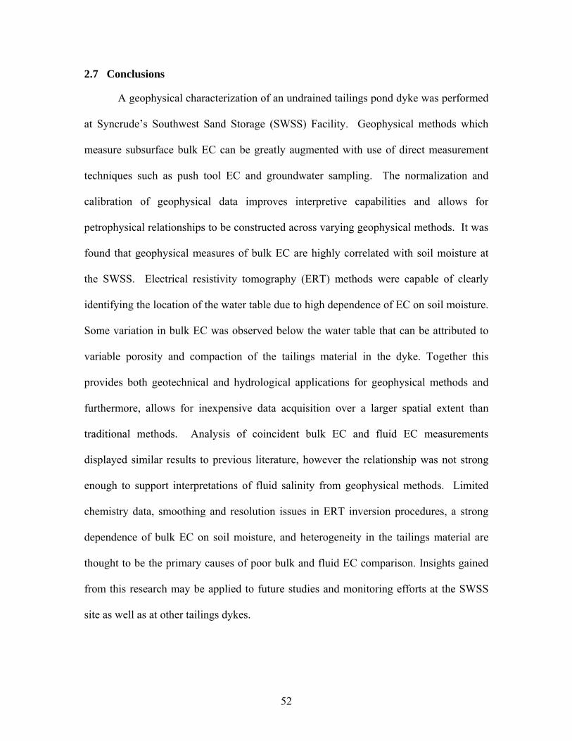
52

2.7 Conclusions

A geophysical characterization of an undrained tailings pond dyke was performed

at Syncrude’s Southwest Sand Storage (SWSS) Facility. Geophysical methods which

measure subsurface bulk EC can be greatly augmented with use of direct measurement

techniques such as push tool EC and groundwater sampling. The normalization and

calibration of geophysical data improves interpretive capabilities and allows for

petrophysical relationships to be constructed across varying geophysical methods. It was

found that geophysical measures of bulk EC are highly correlated with soil moisture at

the SWSS. Electrical resistivity tomography (ERT) methods were capable of clearly

identifying the location of the water table due to high dependence of EC on soil moisture.

Some variation in bulk EC was observed below the water table that can be attributed to

variable porosity and compaction of the tailings material in the dyke. Together this

provides both geotechnical and hydrological applications for geophysical methods and

furthermore, allows for inexpensive data acquisition over a larger spatial extent than

traditional methods. Analysis of coincident bulk EC and fluid EC measurements

displayed similar results to previous literature, however the relationship was not strong

enough to support interpretations of fluid salinity from geophysical methods. Limited

chemistry data, smoothing and resolution issues in ERT inversion procedures, a strong

dependence of bulk EC on soil moisture, and heterogeneity in the tailings material are

thought to be the primary causes of poor bulk and fluid EC comparison. Insights gained

from this research may be applied to future studies and monitoring efforts at the SWSS

site as well as at other tailings dykes.

53

2.8 References

Alberta’s Energy Industry. An Overview. 2012. Alberta Energy Resources Conservation Board. http://www.energy.alberta.ca/org/pdfs/Alberta_Energy_Overview.pdf

Archie, G. 1942. The electrical resistivity log as an aid in determining some reservoir

characteristics. T. Am. I. Min. Met. Eng., Vol. 146. 54 – 62. Bell, J. 1987. Neutron probe practice. 3rd edition. Inst. of Hydrol., Rep. 19. 1 – 63. Berkowitz, N. and Speight, J. 1975. The oil sands of Alberta. Fuel. Vol. 54. 138 – 149. Booterbaugh, A. 2014. Geophysical characterization of an undrained oil sands tailings

pond Alberta, Canada. (Master’s Thesis). Chalaturnyk, R., Scott, D., Özüm, B. 2002. Management of oil sand tailings. Petroleum

Science and Technology. Vol. 20. Nos. 9 & 10. 1025 – 1046. Clark, K. 1929. The separation of the bitumen from Alberta bituminous sands. Can. Inst.

Min. Metall. Bull. Vol. 22. 1385 – 1395. Donaldson, E. and Siddiqui, T. 1989. Relationship between the Archie saturation

exponent and wettability. SPE Form. Eval. 359 – 362. Dusseault, M. and Scott, J. 1983. Tailings pond behavior and characterization of oil sand

tailings sludge. Particulate Science and Technology. Vol. 1. 295 – 309. Hayley, K., Bentley, L, Gharibi, M., Nightingale, M. 2007. Low temperature dependence

of electrical resistivity: Implications for near surface geophysical monitoring. Geophys. Res. Lett. Vol. 34. 1 – 5.

Hayley, K., Bentley, L., Gharibi, M. 2009. Time-lapse electrical resistivity monitoring of

salt-affected soil and groundwater. Water. Resour. Res. Vol. 45. 1 – 14. Heath, R.C., 1983, Basic Ground-water Hydrology: U.S. Geological Survey, 16. Hirsch, M., Bentley, L.R., Dietrich, P. 2008. A comparison of electrical resistivity,

ground penetrating radar and seismic refraction results at a river terrace site. J. Env.and Eng. Geophys., Vol. 13. 325-333.

Hoare, B. 1972. The disposal of mine tailings material. (Doctoral dissertation). University

of Waterloo. 1-210. Kasperski, K. and Mikula, R. 2011. Waste Streams of Mined Oil Sands: Characteristics

and remediation. Elements. Vol. 7. 387 – 392.

54

Komex International Ltd. 2005. 2004 Geophysical Investigation of Southwest Sand Storage Facility. Syncrude Canada Ltd., Fort McMurray, Alberta.

Loke, M. 2006. 1-D frequency domain EM modeling. 115, Cangakay Minden Jalan 5,

11700 Penang, Malaysia. PugSoft Inc. Loke, M., and Barker, R. 1996. Rapid least-squares inversion of apparent resistivity

pseudosections by a quasi-Newton method. Geophys. Prospect. Vol. 44. 131-152. Martínez-Pagán, P., Faz Cano, A., Aracil, E., Arocena, J. 2009. Electrical resistivity

imaging revealed the spatial properties of mine tailing ponds in Sierra Minera of southeast Spain. J. Environ. Eng. Geoph. Vol. 14, 2. 63 – 76.

Masliyah, J., Zhou, Z., Xu, Z., Czarnecki, J., Hamza, H. 2004. Understanding water-

based bitumen extraction from Athabasca Oil Sands. Can. J. Chem. Eng. Vol. 82. 628 – 654.

Meads, L.N., Bentley, L.R., Mendoza, C.A. 2003. Application of electrical resistivity

imaging to the development of a geologic model for a proposed Edmonton landfill site. Can. Geotech. J. Vol. 40. 551-558.

Morgan, W. and Pirson, S. 1964. The effect of fractional wettability on the Archie

saturation exponent. SPWLA 5th Annual Logging Symposium. 1 – 13. Naeth, M., Chanasyk, D., Burgers, T. 2011. Vegetation and soil water interactions on a

tailings sand storage facility in the Athabasca oil sands region of Alberta Canada. Phys. Chem. Earth. Vol. 36. 19-30.

Price, A. 2005. Evaluation of groundwater flow and salt transport within an undrained

tailings sand dam (Master’s Thesis). University of Alberta, Department of Earth and Atmospheric Sciences.

Roy, A., Apparao, A. 1971. Depth of investigation in direct current methods. Geophysics.

Vol. 36, No. 5. 943 -959. Singha, K., Gorelick, S. 2006. Effects of spatially variable resolution on field-scale

estimates of tracer concentration from electrical inversions using Archies’s law. Geophysics. Vol. 71, No. 3. G83 – G91.

Sjödahl, P., Dahlin, T., Johansson, S. 2005. Using resistivity measurements for dam

safety evaluation at Ememossen tailings dam in southern Sweden. Environ. Geol. Vol. 49. 267 – 273.

Sweeney, S. and Jennings, H. 1960. Effect of wettability on the electrical resistivity of

carbonate rock from a petroleum reservoir. J. Phys. Chem. Vol. 64. No. 5. 551 – 553.

55

Syncrude Canada Ltd.. 2008. Public Disclosure Document: South west sand storage

Conversion. Tóth, J. 1963. A theoretical analysis of groundwater flow in small drainage basins. J.

Geophys. Res. Vol. 68, No. 16. 4795 – 4812. Yuval, D. and Oldenburg, W. 1996. DC resistivity and IP methods in acid mind drainage

problems: results from the Copper Cliff mine tailings impoundments. J. Appl. Geophys. Vol. 34. 187 – 198.

56

Table 2.1. Summary statistics for normalization example displayed in Figure 2.3. EM regions are labeled in the same fashion (regions X, Y, & Z) as seen in Figure 2.3.

Elevated Region

Reference Region (Z) Pre-normalization (X) Post-normalization (Y) Max 452 444.99 440 Min 137 67.74 59

Mean 224.13 162.98 162.99 Median 213 133.27 133

Variance 2608.09 4721.76 4736.25

57

Table 2.2. Manually optimized inversion parameters selected for ERT modeling.

Parameter Value

Data norm L1 Model norm L1 Vertical to horizontal flatness filter ratio 0.25 Initial damping factor 0.1 Minimum damping factor 0.04 Increase damping factor with depth 1.1 Model block width 0.5 m Model first layer height 0.125 m Rate of layer height increase with depth 1.05

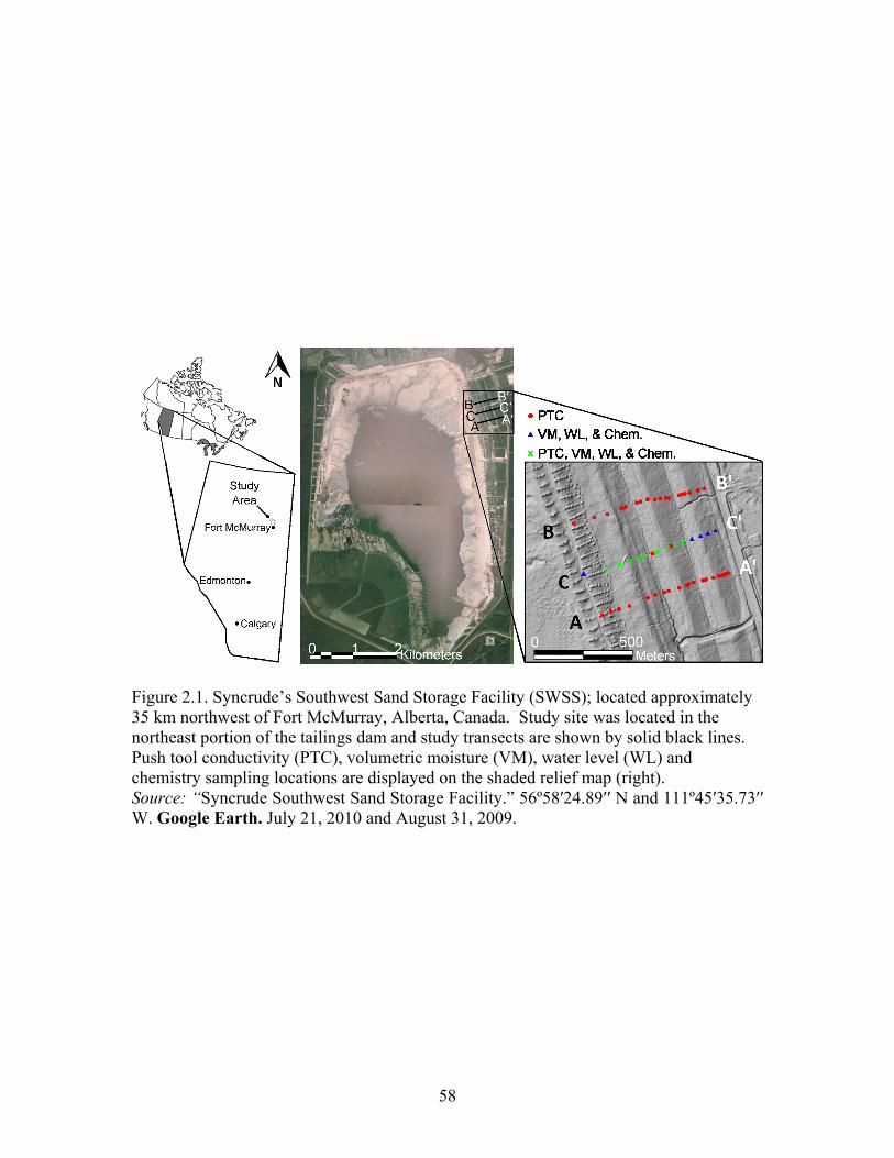
58

Figure 2.1. Syncrude’s Southwest Sand Storage Facility (SWSS); located approximately 35 km northwest of Fort McMurray, Alberta, Canada. Study site was located in the northeast portion of the tailings dam and study transects are shown by solid black lines. Push tool conductivity (PTC), volumetric moisture (VM), water level (WL) and chemistry sampling locations are displayed on the shaded relief map (right). Source: “Syncrude Southwest Sand Storage Facility.” 56º58′24.89′′ N and 111º45′35.73′′ W. Google Earth. July 21, 2010 and August 31, 2009.

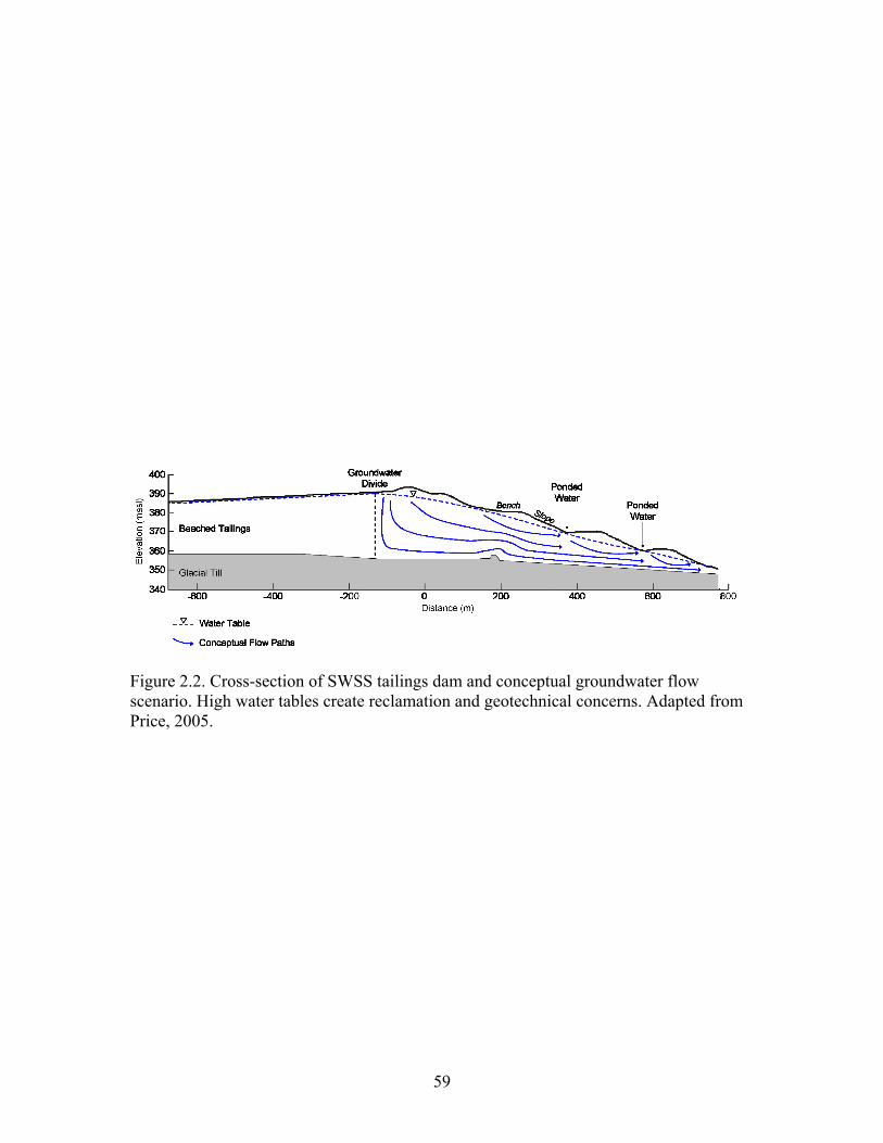
59

Figure 2.2. Cross-section of SWSS tailings dam and conceptual groundwater flow scenario. High water tables create reclamation and geotechnical concerns. Adapted from Price, 2005.

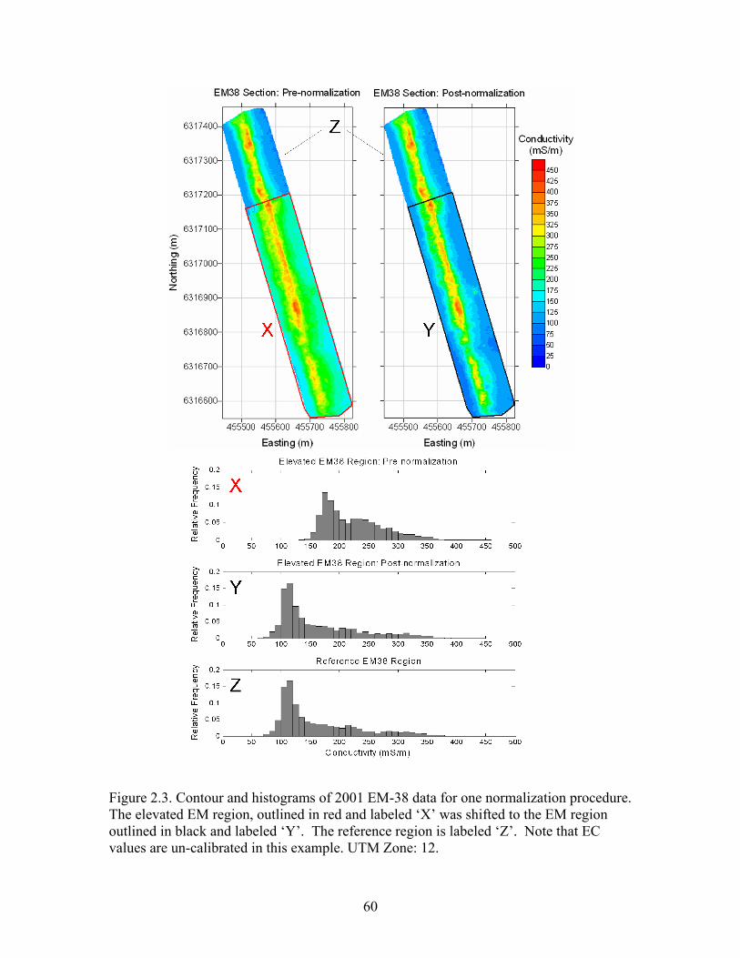
60

Figure 2.3. Contour and histograms of 2001 EM-38 data for one normalization procedure. The elevated EM region, outlined in red and labeled ‘X’ was shifted to the EM region outlined in black and labeled ‘Y’. The reference region is labeled ‘Z’. Note that EC values are un-calibrated in this example. UTM Zone: 12.

61

0 100 2000

20

40

60

80

100

Ca

lcu

late

d E

M C

on

du

ctiv

ity (

mS

/m)

Measured EM Conductivity (mS/m)

EM38 Calibration 2001

0 100 2000

20

40

60

80

100

Measured EM Conductivity (mS/m)

EM38 Calibration 2004

Ca

lcu

late

d E

M C

on

du

ctiv

ity (

mS

/m)

Figure 2.4. Calibration crossplots for EM-38 data from 2001 (left) and 2004 (right). Linear regression with y-intercept equal to zero was used to calibrate EM-38 EC measurements. Regression slopes varied significantly between 2001 and 2004; 0.420 and 1.33, respectively. R2 values are 0.61 and 0.88 for 2001 and 2004, respectively. Note, regressions are site specific.

62

0 50 100 1500

50

100

150

200

ERT Conductivity (mS/m)

PT

C C

on

du

ctiv

ity (

mS

/m)

ERT Calibration 2004

0 50 100 1500

50

100

150

200

PT

C C

on

du

ctiv

ity (

mS

/m)

ERT Calibration 2001

ERT Conductivity (mS/m) Figure 2.5. Calibration cross-plots for ERT data from 2001 (left) and 2004 (right). Linear regression with y-intercept equal to zero was used for the calibration model. Slopes for linear regression of 2001 and 2004 data are 1.46 and 1.40, respectively. R2 values are 0.64 and 0.52 for 2001 and 2004, respectively. Note, regressions are site specific

63

Figure 2.6. EM-38 normalized and calibrated EC image collected in the fall of 2001. EM-38 was collected over a large area of the SWSS tailings dam. Study transects are shown by black dashed lines. UTM Zone: 12.

64

Figure 2.7. EM-38 normalized and calibrated EC image collected in the fall of 2004. EM-38 was only implemented in a small vicinity of study transects A and C, shown by black dashed lines. UTM Zone: 12.

65

Figure 2.8. EM-38 normalized and calibrated EC data from fall of 2004 plotted along a cross-section of transect A to A′.

66

Figure 2.9. Electrical resistivity tomography for transect C from fall 2004 (A) and fall of 2008 (B). Coincidental water level measurements are superimposed. A difference plot is also shown (C) for 2008 minus 2004; mean absolute difference of 4.3 mS/m was found.

0 100 200 300 400 500 600 700 800340

350

360

370

380

390

Distance (m)

Ele

vatio

n (

ma

sl)

Transect C Difference Plot: 2008 - 2004

Co

nd

uct

ivity

Diff

ere

nce

(m

S/m

)

-100

-50

0

50

100

0 100 200 300 400 500 600 700 800340

350

360

370

380

390

Ele

vatio

n (

ma

sl)

ERT Transect C 2008

Co

nd

uct

ivity

(m

S/m

)

0.3

1

3.2

10

31.6

100

316.2

0 100 200 300 400 500 600 700 800340

350

360

370

380

390

Ele

vatio

n (

ma

sl)

ERT Transect C 2004

Co

nd

uct

ivity

(m

S/m

)

0.3

1

3.2

10

31.6

100

316.2Water Table (Linear Interpolation)Water Table Measurements

C

C′

C

C′

C

C′

A 

B 

C 

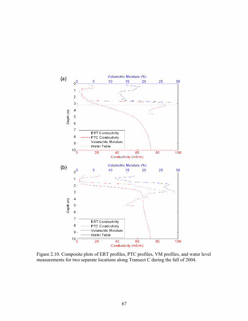
67

Figure 2.10. Composite plots of ERT profiles, PTC profiles, VM profiles, and water level measurements for two separate locations along Transect C during the fall of 2004.

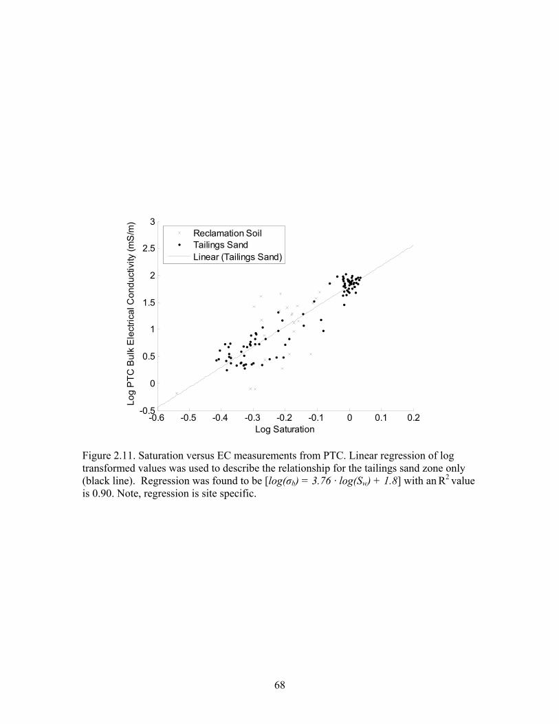
68

-0.6 -0.5 -0.4 -0.3 -0.2 -0.1 0 0.1 0.2-0.5

0

0.5

1

1.5

2

2.5

3

Log Saturation

Lo

g P

TC

Bu

lk E

lect

rica

l Co

nd

uctiv

ity (

mS

/m)

Reclamation SoilTailings SandLinear (Tailings Sand)

Figure 2.11. Saturation versus EC measurements from PTC. Linear regression of log transformed values was used to describe the relationship for the tailings sand zone only (black line). Regression was found to be [log(σb) = 3.76 · log(Sw) + 1.8] with an R

2 value is 0.90. Note, regression is site specific.

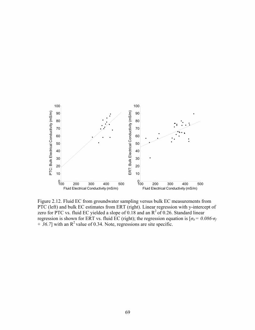
69

100 200 300 400 5000

10

20

30

40

50

60

70

80

90

100

Fluid Electrical Conductivity (mS/m)

PT

C: B

ulk

Ele

ctri

cal C

on

du

ctiv

ity (

mS

/m)

100 200 300 400 5000

10

20

30

40

50

60

70

80

90

100

Fluid Electrical Conductivity (mS/m)

ER

T: B

ulk

Ele

ctri

cal C

on

du

ctiv

ity (

mS

/m)

Figure 2.12. Fluid EC from groundwater sampling versus bulk EC measurements from PTC (left) and bulk EC estimates from ERT (right). Linear regression with y-intercept of zero for PTC vs. fluid EC yielded a slope of 0.18 and an R2 of 0.26. Standard linear regression is shown for ERT vs. fluid EC (right); the regression equation is [σb = 0.086·σf + 36.7] with an R2 value of 0.34. Note, regressions are site specific.

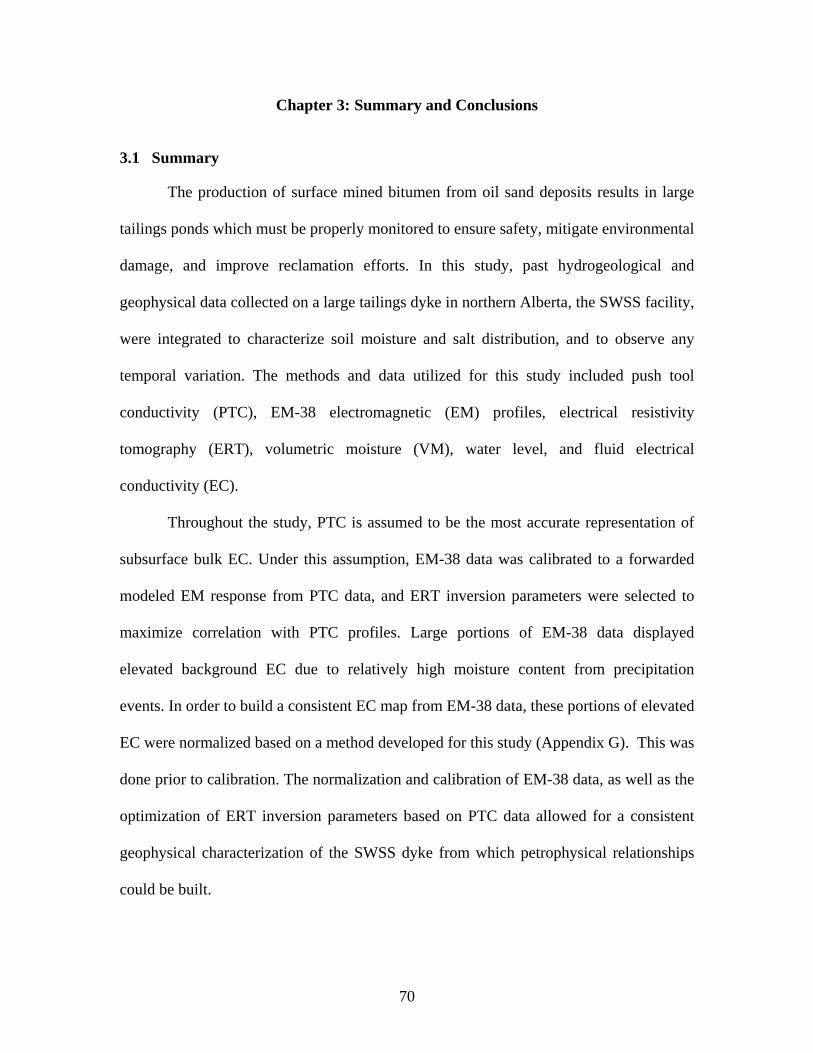
70

Chapter 3: Summary and Conclusions

3.1 Summary

The production of surface mined bitumen from oil sand deposits results in large

tailings ponds which must be properly monitored to ensure safety, mitigate environmental

damage, and improve reclamation efforts. In this study, past hydrogeological and

geophysical data collected on a large tailings dyke in northern Alberta, the SWSS facility,

were integrated to characterize soil moisture and salt distribution, and to observe any

temporal variation. The methods and data utilized for this study included push tool

conductivity (PTC), EM-38 electromagnetic (EM) profiles, electrical resistivity

tomography (ERT), volumetric moisture (VM), water level, and fluid electrical

conductivity (EC).

Throughout the study, PTC is assumed to be the most accurate representation of

subsurface bulk EC. Under this assumption, EM-38 data was calibrated to a forwarded

modeled EM response from PTC data, and ERT inversion parameters were selected to

maximize correlation with PTC profiles. Large portions of EM-38 data displayed

elevated background EC due to relatively high moisture content from precipitation

events. In order to build a consistent EC map from EM-38 data, these portions of elevated

EC were normalized based on a method developed for this study (Appendix G). This was

done prior to calibration. The normalization and calibration of EM-38 data, as well as the

optimization of ERT inversion parameters based on PTC data allowed for a consistent

geophysical characterization of the SWSS dyke from which petrophysical relationships

could be built.

71

The Archie’s Law petrophysical model was used in this study and relates bulk

EC, fluid EC, and soil-moisture in a clay-free porous medium. Through the relationship

with bulk EC and VM, as well as bulk EC and fluid EC, it was possible to provide

estimates for Archie’s saturation exponent (n = 3.8) and formation factor respectively (F

= 0.18). To complete this model, a porosity of 26.9% was estimated as the average VM

from the fully saturated zone, and a cementation factor (m = 1.3) was assumed based on

literature. Bulk EC and VM relationships displayed a strong correlation (R2 = 0.90).

Conversely, bulk and fluid EC relationships displayed relatively weak correlations with a

R2 of 0.26 for PTC versus fluid EC, and a R2 of 0.34 for ERT versus fluid EC; although in

general agreed with previous literature for formation factor estimates. Limited chemistry

data, sample support discrepancies, ERT resolution issues, a strong dependence of bulk

EC on soil-moisture, and heterogeneity in the tailings material which forms the dyke are

thought to be the cause of weak correlation between bulk and fluid EC.

3.2 Conclusions

The results of this research show a strong correlation between bulk EC and soil-

moisture at the SWSS dyke. Geophysical methods utilized in this study, which provide

measurements of bulk EC, can therefore provide soil-moisture estimates in a non-

intrusive manner over a much larger spatial extent than traditional invasive measurement

techniques. This relationship has geotechnical and environmental relevance, especially at

tailings sites similar to the SWSS facility where high water tables present both safety and

reclamation concerns. The normalization and calibration of the EM-38 data, as well as

the optimization of ERT inversion parameters using the correlation to PTC profiles is a

valuable step to ensure each technique displays similar magnitudes and distributions of

72

bulk EC. This allows for consistent petrophysical relationships to be constructed across

varying geophysical methods.

ERT methods clearly identified the location of the water table within the SWSS

dyke, due to a high dependence of measured bulk EC on soil moisture. This is significant

as it allows for a spatially exhaustive water level measurement in a much more rapid and

non-invasive manner than the installation of water level monitoring wells. The

installation of several water level wells may be useful for defining a precise water level

location within the smoothed tomogram produced through ERT inversion. Regardless,

ERT should be considered a very useful tool in this setting for not only geotechnical

application, but also for use in calibrating groundwater flow models.

Geophysical methods, namely PTC and ERT, were incapable of resolving salinity

changes or providing any reasonable quantitative estimates of fluid EC at the SWSS

facility. The ability to resolve salinity was limited by insufficient coincidental bulk and

fluid EC data, especially in PTC based relationships, as well as ERT smoothing,

resolution, heterogeneity in the tailings material, and sample support issues. Furthermore,

the strong dependence of bulk EC on soil moisture may have masked salinity variations

within the SWSS dyke. That being said, bulk versus fluid EC relationships which were

formed, albeit with weak correlation, displayed estimates for the Archie Law formation

factor which were similar to literature values. To improve upon the correlation between

bulk and fluid EC, future studies should be designed to greatly increase the number of

coincidental measurements of these two parameters. Furthermore, detailed temperature

profiling is vital for quantitative interpretations to be made from electrical geophysical

techniques. A flow and heat transport model as well as a dense temperature measurement

73

program are recommended to adequately characterize the complex nature of the

temperature distribution at this site.

3.3 Future Work

In 2009, the design of the SWSS dyke was altered to a centerline dyke

construction method which includes internal drainage. These changes most likely had

large impacts on the groundwater flow regime and salt transport within the structure.

With this said, the research conducted in this study, and previously, present both the

applicability and limitations of various integrated methods in characterizing soil moisture

and salinity within oil sand tailings dams. The insights gained from this process may be

applied to improve not only future monitoring at the SWSS facility, but also other tailings

dams of similar nature. The high dependence of measured bulk EC on soil moisture in the

SWSS presents the opportunity to use geophysical methods to calibrate and validate

future groundwater flow models at the SWSS and other tailings dams. Future work which

uses geophysical data for this purpose is highly recommended. Furthermore, future

research should be conducted to better understand and define bulk versus fluid EC

relationships in tailings pond dykes. Such information could be used to improve upon

future transport modeling and overall enhance the management and reclamation of

tailings ponds.

74

Appendix A: Push Tool Conductivity Figures & Data

Data for PTC data may be found in the attached material, in folder ‘Appendix A’. Data files are separated

by year, and the transect location is included in the file name; e.g. ‘PTCA2001.txt’ represents PTC data

from Transect A in 2001.

0 100 200 300 400 500 600 700 800350

360

370

380

390

400

21

2223 24

2526

27 28 2930

3132

3334 353637

3839

Distance (m)

Ele

vatio

n (m

asl)

Transect A

Figure A1. PTC locations and identification along Transect A.

75

0 100 200 300 400 500 600 700 800350

360

370

380

390

400

Distance (m)

Ele

vatio

n (m

asl)

Transect B

1

2 3

4 7

8 9 1011

121314

151617 18

1920

Figure A2. PTC locations and identification along Transect B.

0 100 200 300 400 500 600 700 800350

360

370

380

390

400

Distance (m)

Ele

vatio

n (m

asl)

Transect C

101

102103104

105106

107108109

110

111112113

115

Figure A3. PTC and groundwater well locations, and identification along Transect C.

76

0 50 100 150

0

1

2

3

4

5

6

Dep

th (

m)

PTC 1

0 50 100 150

0

1

2

3

4

5

6

Dep

th (

m)

PTC 3

0 20 40 60 80 100

0

1

2

3

4

5

PTC 4

0 50 100 150

0

1

2

3

4

5

Dep

th (

m)

Conductivity (mS/m)

PTC 7

0 20 40 60 80 100

0

1

2

3

4

5

Conductivity (mS/m)

PTC 8

0 20 40 60 80 100

0

1

2

3

4

5

6

PTC 2

Raw

5pt Smooth

A4 A5

A8 A9

A6 A7

77

0 20 40 60 80 100

0

1

2

3

4

5

Dep

th (

m)

PTC 9

0 10 20 30 40

0

1

2

3

4

5

PTC 10

0 20 40 60 80

0

1

2

3

4

5

Dep

th (

m)

PTC 11

0 20 40 60 80 100

0

1

2

3

4

5

PTC 12

0 20 40 60 80

0

1

2

3

4

5

Conductivity (mS/m)

Dep

th (

m)

PTC 13

0 50 100 150

0

1

2

3

4

5

Conductivity (mS/m)

PTC 14

Raw

5pt Smooth

A12 A13

A14 A15

A10 A11

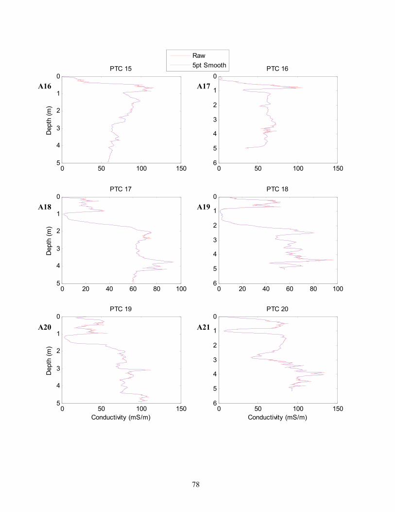
78

0 50 100 150

0

1

2

3

4

5

Dep

th (

m)

PTC 15

0 50 100 150

0

1

2

3

4

5

6

PTC 16

0 20 40 60 80 100

0

1

2

3

4

5

Dep

th (

m)

PTC 17

0 20 40 60 80 100

0

1

2

3

4

5

6

PTC 18

0 50 100 150

0

1

2

3

4

5

Conductivity (mS/m)

Dep

th (

m)

PTC 19

0 50 100 150

0

1

2

3

4

5

6

Conductivity (mS/m)

PTC 20

Raw

5pt Smooth

A18 A19

A20 A21

A16 A17

79

0 50 100 150

0

1

2

3

4

5

Dep

th (

m)

PTC 21

0 50 100 150

0

1

2

3

4

5

6

PTC 22

0 20 40 60 80 100

0

1

2

3

4

5

Dep

th (

m)

PTC 23

0 50 100 150

0

1

2

3

4

5

6

PTC 24

0 20 40 60 80 100

0

1

2

Conductivity (mS/m)

Dep

th (

m)

PTC 25

0 20 40 60 80 100

0

1

2

3

4

5

Conductivity (mS/m)

PTC 26

Raw

5pt Smooth

A24 A25

A26 A27

A22 A23

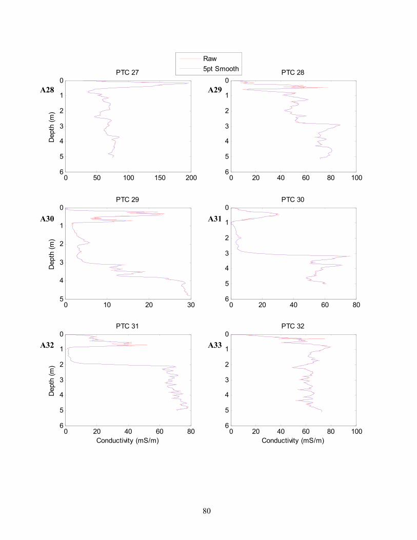
80

0 50 100 150 200

0

1

2

3

4

5

6

Dep

th (

m)

PTC 27

0 20 40 60 80 100

0

1

2

3

4

5

6

PTC 28

0 10 20 30

0

1

2

3

4

5

Dep

th (

m)

PTC 29

0 20 40 60 80

0

1

2

3

4

5

6

PTC 30

0 20 40 60 80

0

1

2

3

4

5

6

Conductivity (mS/m)

Dep

th (

m)

PTC 31

0 20 40 60 80 100

0

1

2

3

4

5

6

Conductivity (mS/m)

PTC 32

Raw

5pt Smooth

A30 A31

A32 A33

A28 A29

81

0 50 100 150 200

0

1

2

3

4

5

6

Dep

th (

m)

PTC 33

0 20 40 60 80

0

1

2

3

4

5

6

PTC 34

0 20 40 60 80

0

1

2

3

4

5

6

Dep

th (

m)

PTC 35

0 20 40 60 80

0

1

2

3

4

5

6

PTC 36

0 20 40 60 80

0

1

2

3

4

5

Conductivity (mS/m)

Dep

th (

m)

PTC 37

0 50 100 150 200

0

1

2

3

4

5

6

Conductivity (mS/m)

PTC 38

Raw

5pt Smooth

A36 A37

A38 A39

A34 A35

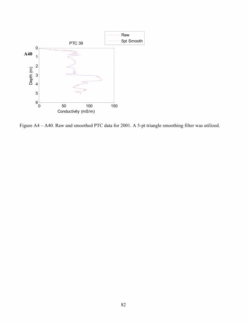
82

0 50 100 150

0

1

2

3

4

5

6

Conductivity (mS/m)

Dep

th (

m)

PTC 39

Raw

5pt Smooth

Figure A4 – A40. Raw and smoothed PTC data for 2001. A 5-pt triangle smoothing filter was utilized.

A40

83

0 20 40 60 80 100

0

1

2

3

4

5

Dep

th (

m)

PTC 110

0 20 40 60 80 100

0

1

2

3

4

5

PTC 109

0 10 20 30

0

1

2

3

4

Dep

th (

m)

PTC 111

0 20 40 60 80 100

0

1

2

3

4

5

PTC 108

0 20 40 60

0

1

2

3

4

5

Conductivity (mS/m)

Dep

th (

m)

PTC 107

0 20 40 60 80 100

0

1

2

3

4

5

Conductivity (mS/m)

PTC 106

Raw

5pt Smooth

A43 A44

A45 A46

A41 A42

84

0 50 100 150

0

1

2

3

4

5

Dep

th (

m)

PTC 105

0 20 40 60 80 100

0

1

2

3

4

5

PTC 23

0 20 40 60 80 100

0

1

2

3

4

5

Dep

th (

m)

PTC 24

0 50 100 150

0

1

2

3

4

5

PTC 25

50 100 150 200 250

0

1

2

3

4

5

Conductivity (mS/m)

Dep

th (

m)

PTC 27

0 20 40 60 80 100

0

1

2

3

4

5

Conductivity (mS/m)

PTC 28

Raw

5pt Smooth

A49 A50

A51 A52

A47 A48

85

0 20 40 60 80

0

1

2

3

4

5

Dep

th (

m)

PTC 29

0 20 40 60 80 100

0

1

2

3

4

5

PTC 30

0 20 40 60 80

0

1

2

3

4

5

Conductivity (mS/m)

Dep

th (

m)

PTC 31

20 40 60 80 100 120

0

1

2

3

4

5

Conductivity (mS/m)

PTC 32

Raw

5pt Smooth

Figure A41 – A56. Raw and smoothed PTC data for 2004. A 5-pt triangle smoothing filter was utilized.

A55 A56

A53 A54

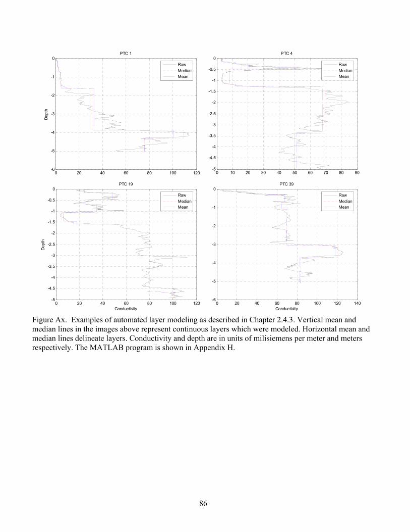
86

Figure Ax. Examples of automated layer modeling as described in Chapter 2.4.3. Vertical mean and median lines in the images above represent continuous layers which were modeled. Horizontal mean and median lines delineate layers. Conductivity and depth are in units of milisiemens per meter and meters respectively. The MATLAB program is shown in Appendix H.

0 20 40 60 80 100 120-6

-5

-4

-3

-2

-1

0

Dep

th

PTC 1

Raw

MedianMean

0 10 20 30 40 50 60 70 80 90-5

-4.5

-4

-3.5

-3

-2.5

-2

-1.5

-1

-0.5

0PTC 4

Raw

MedianMean

0 20 40 60 80 100 120-5

-4.5

-4

-3.5

-3

-2.5

-2

-1.5

-1

-0.5

0

Conductivity

Dep

th

PTC 19

Raw

MedianMean

0 20 40 60 80 100 120 140-6

-5

-4

-3

-2

-1

0

Conductivity

PTC 39

Raw

MedianMean

87

Appendix B: EM-38 Data

The raw, normalized, and calibrated EM-38 data may be found in the attached material, in folder

‘Appendix B’. The data is organized by survey year. Only data collected in the vertical dipole mode are

given, as horizontal data was not reported in this study and not collected in 2004.

88

Appendix C: Electrical Resistivity Tomography Figures & Data

Raw and inverted ERT data may be found in attached material, in folder ‘Appendix C’. Raw data is

formatted for Res2DInv and includes complete topography from a 1 meter DEM. Inverted data is given as

a four column matrix with distance (m), elevation (masl), resistivity (Ohm.m), and conductivity (S/m)

respectively. Files are labeled with transect and year, e.g. ‘Raw ERTA 2001.txt’ represents raw ERT data

from Transect A, surveyed during 2001.

Figure C1. Inverted ERT cross-section for Transect A; data collected in 2001.

Figure C2. Inverted ERT cross-section for Transect B; data collected in 2001.

89

Figure C3. Inverted ERT cross-section for Transect A; data collected in 2004.

Figure C4. Inverted ERT cross-section for Transect C; data collected in 2004.

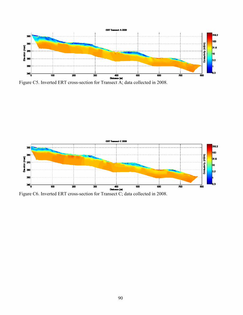
90

Figure C5. Inverted ERT cross-section for Transect A; data collected in 2008.

Figure C6. Inverted ERT cross-section for Transect C; data collected in 2008.

91

Figure C7. ERT difference plot for 2004 minus 2001 along Transect A.

Figure C8. ERT difference plot for 2008 minus 2004 along Transect A.

92

Figure C9. ERT difference plot for 2008 minus 2004 along Transect C.

93

Appendix D: Volumetric Moisture from Neutron Probe Figures & Data

Volumetric moisture data can be found in attached material, in folder ‘Appendix D’. Data files are labeled

by survey location, e.g. ‘gw1.txt’. The first row displays the date of each survey at a given location in

Julian days; the underlining column represents the volumetric moisture data for a given Julian date. The

first column represents depth, measured in centimeters.

0 100 200 300 400 500 600 700 800350

355

360

365

370

375

380

385

390

395

Distance (m)

Ele

vatio

n (m

asl)

Line C Cross-section Survey

1

234

5

6

789

10

1112

13

15

Figure D1. Location of groundwater sampling wells (GW) and neutron probe access tubes along Transect C. (Note: Appendix A utilized different identification numbers to prevent confusion with PTC data from other transects.)

94

20 25 30 35

0

50

100

150

200

250

300

Average Volumetric Moisture %

Dep

th (

cm)

Apr01 Jan04 Oct06 Jul09 Apr12 Dec14

0

50

100

150

200

250

300

Time (days)

Dep

th (

cm)

GW 1

10

15

20

25

30

35

40

Figure D2. Volumetric moisture from neutron probe data from GW1. The average volumetric moisture for all profiles taken at the specified location is shown on the left. The image on the right displays volumetric moisture profiles through time with hot colors indicating low moisture and cool colors indicating high moisture.

10 15 20 25 30

0

50

100

150

200

250

300

Average Volumetric Moisture %

Dep

th (

cm)

Jan04 Aug04 Feb05 Sep05 Mar06 Oct06 Apr07 Nov07

0

50

100

150

200

250

300

Time (days)

Dep

th (

cm)

GW 2

10

12

14

16

18

20

22

24

26

28

Figure D3. Volumetric moisture from neutron probe data from GW2. The average volumetric moisture for all profiles taken at the specified location is shown on the left. The image on the right displays volumetric moisture profiles through time with hot colors indicating low moisture and cool colors indicating high moisture.

95

10 15 20 25 30

0

50

100

150

200

250

300

Average Volumetric Moisture %

Dep

th (

cm)

Jan04 Aug04 Feb05 Sep05 Mar06 Oct06 Apr07 Nov07

0

50

100

150

200

250

300

Time (days)

Dep

th (

cm)

GW 3

10

15

20

25

30

Figure D4. Volumetric moisture from neutron probe data from GW3. The average volumetric moisture for all profiles taken at the specified location is shown on the left. The image on the right displays volumetric moisture profiles through time with hot colors indicating low moisture and cool colors indicating high moisture.

0 10 20 30 40

0

50

100

150

200

250

300

Average Volumetric Moisture %

Dep

th (

cm)

Jan04 Aug04 Feb05 Sep05 Mar06 Oct06 Apr07 Nov07

0

50

100

150

200

250

300

Time (days)

Dep

th (

cm)

GW 4

5

10

15

20

25

30

35

Figure D5. Volumetric moisture from neutron probe data from GW4. The average volumetric moisture for all profiles taken at the specified location is shown on the left. The image on the right displays volumetric moisture profiles through time with hot colors indicating low moisture and cool colors indicating high moisture.

96

15 20 25 30 35

0

50

100

150

200

250

300

Average Volumetric Moisture %

Dep

th (

cm)

Apr01 Sep02 Jan04 May05 Oct06 Feb08 Jul09 Nov10

0

50

100

150

200

250

300

Time (days)

Dep

th (

cm)

GW 5

10

15

20

25

30

35

40

Figure D6. Volumetric moisture from neutron probe data from GW5. The average volumetric moisture for all profiles taken at the specified location is shown on the left. The image on the right displays volumetric moisture profiles through time with hot colors indicating low moisture and cool colors indicating high moisture.

10 15 20 25 30

0

50

100

150

200

250

300

Average Volumetric Moisture %

Dep

th (

cm)

Jan04 Aug04 Feb05 Sep05 Mar06 Oct06 Apr07 Nov07

0

50

100

150

200

250

300

Time (days)

Dep

th (

cm)

GW 6

8

10

12

14

16

18

20

22

24

26

28

Figure D7. Volumetric moisture from neutron probe data from GW6. The average volumetric moisture for all profiles taken at the specified location is shown on the left. The image on the right displays volumetric moisture profiles through time with hot colors indicating low moisture and cool colors indicating high moisture.

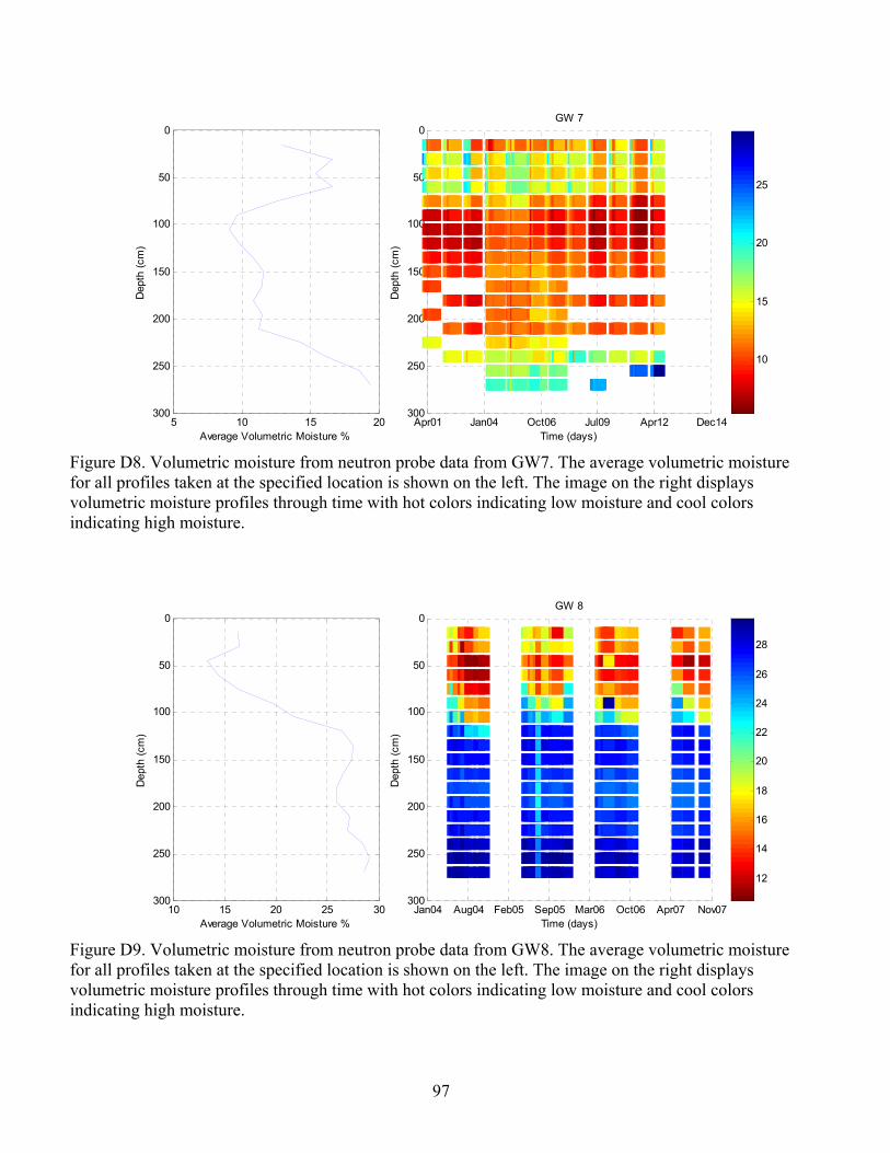
97

5 10 15 20

0

50

100

150

200

250

300

Average Volumetric Moisture %

Dep

th (

cm)

Apr01 Jan04 Oct06 Jul09 Apr12 Dec14

0

50

100

150

200

250

300

Time (days)

Dep

th (

cm)

GW 7

10

15

20

25

Figure D8. Volumetric moisture from neutron probe data from GW7. The average volumetric moisture for all profiles taken at the specified location is shown on the left. The image on the right displays volumetric moisture profiles through time with hot colors indicating low moisture and cool colors indicating high moisture.

10 15 20 25 30

0

50

100

150

200

250

300

Average Volumetric Moisture %

Dep

th (

cm)

Jan04 Aug04 Feb05 Sep05 Mar06 Oct06 Apr07 Nov07

0

50

100

150

200

250

300

Time (days)

Dep

th (

cm)

GW 8

12

14

16

18

20

22

24

26

28

Figure D9. Volumetric moisture from neutron probe data from GW8. The average volumetric moisture for all profiles taken at the specified location is shown on the left. The image on the right displays volumetric moisture profiles through time with hot colors indicating low moisture and cool colors indicating high moisture.

98

15 20 25 30

0

50

100

150

200

250

300

Average Volumetric Moisture %

Dep

th (

cm)

Jan04 Aug04 Feb05 Sep05 Mar06 Oct06 Apr07 Nov07

0

50

100

150

200

250

300

Time (days)

Dep

th (

cm)

GW 9

10

12

14

16

18

20

22

24

26

28

Figure D10. Volumetric moisture from neutron probe data from GW9. The average volumetric moisture for all profiles taken at the specified location is shown on the left. The image on the right displays volumetric moisture profiles through time with hot colors indicating low moisture and cool colors indicating high moisture.

10 15 20 25 30

0

50

100

150

200

250

300

Average Volumetric Moisture %

Dep

th (

cm)

Jan04 Aug04 Feb05 Sep05 Mar06 Oct06 Apr07 Nov07

0

50

100

150

200

250

300

Time (days)

Dep

th (

cm)

GW 10

10

15

20

25

30

Figure D11. Volumetric moisture from neutron probe data from GW10. The average volumetric moisture for all profiles taken at the specified location is shown on the left. The image on the right displays volumetric moisture profiles through time with hot colors indicating low moisture and cool colors indicating high moisture.

99

5 10 15 20 25

0

50

100

150

200

250

300

Average Volumetric Moisture %

Dep

th (

cm)

Jan04 Aug04 Feb05 Sep05 Mar06 Oct06 Apr07 Nov07

0

50

100

150

200

250

300

Time (days)

Dep

th (

cm)

GW 11

5

10

15

20

25

Figure D12. Volumetric moisture from neutron probe data from GW11. The average volumetric moisture for all profiles taken at the specified location is shown on the left. The image on the right displays volumetric moisture profiles through time with hot colors indicating low moisture and cool colors indicating high moisture.

15 20 25 30

0

50

100

150

200

250

300

Average Volumetric Moisture %

Dep

th (

cm)

Jan04 Aug04 Feb05 Sep05 Mar06 Oct06 Apr07 Nov07

0

50

100

150

200

250

300

Time (days)

Dep

th (

cm)

GW 12

10

12

14

16

18

20

22

24

26

28

Figure D13. Volumetric moisture from neutron probe data from GW12. The average volumetric moisture for all profiles taken at the specified location is shown on the left. The image on the right displays volumetric moisture profiles through time with hot colors indicating low moisture and cool colors indicating high moisture.

100

10 15 20 25 30 35

0

50

100

150

200

250

Average Volumetric Moisture %

Dep

th (

cm)

Jan04 Aug04 Feb05 Sep05 Mar06 Oct06 Apr07 Nov07

0

50

100

150

200

250

Time (days)

Dep

th (

cm)

GW 13

10

15

20

25

30

Figure D14. Volumetric moisture from neutron probe data from GW13. The average volumetric moisture for all profiles taken at the specified location is shown on the left. The image on the right displays volumetric moisture profiles through time with hot colors indicating low moisture and cool colors indicating high moisture.

5 10 15 20 25

0

50

100

150

200

250

300

Average Volumetric Moisture %

Dep

th (

cm)

Jan04 Aug04 Feb05 Sep05 Mar06 Oct06 Apr07 Nov07

0

50

100

150

200

250

300

Time (days)

Dep

th (

cm)

GW 15

10

15

20

25

30

Figure D15. Volumetric moisture from neutron probe data from GW15. The average volumetric moisture for all profiles taken at the specified location is shown on the left. The image on the right displays volumetric moisture profiles through time with hot colors indicating low moisture and cool colors indicating high moisture.

101

Appendix E: Water Level Data

Water level measurements that were collected during similar times as geophysical data for 2004 and 2008

can be found in attached materials, in folder ‘Appendix E’. The folder contains a .txt file which contains

the water level data utilized in this study.

102

Appendix F: Fluid Electrical Conductivity Data

Fluid electrical conductivity data and other chemistry data collected along Transect C may be found in

attached materials, in folder ‘Appendix F’. The folder contains a .txt file that holds all chemistry data

collected along Transect C and investigated in this study. For the results of this research, fluid EC was the

primary parameter of concern. However, with the inability to resolve fluid EC from geophysics and build

strong relationships between the two, many other parameters (TDS, major anion and cations, etc.) were

excluded as they did not provide any further insight towards the study’s objective.

103

Appendix G: EM-38 Normalization MATLAB Script

The following is the script for the EM-38 normalization procedure discussed in Chapter 2.4.4. The script

is written in the MATLAB programming language. The user must input data for the elevated region as

‘elef’ and for the reference region as ‘normf’. Furthermore, the user can set the number of desired

quantiles in which to divide each data set into. This can be achieved by changing the assigned value of

variable ‘q’ in line 8. A value of 100 was used in this study and found to produce reasonable results. The

variable ‘shift_ele’ defined while running the script, represents the normalized elevated data set. The

original elevated data ‘elef’ may be replaced with ‘shift_ele’ to produce a final normalized section.

EM-38 Normalization Script %% Quantiles split %normf - zone of reference or non-elevated EM data %elef - zone of elevated EM data %Both normf and elef must represent areas that should be statistically stationary for %normalization process to work. q = 100; % Number of desired quantiles ne = length(elef); nn = length(normf); neq = ne/q; %number of data per elevated data quantile nnq = nn/q; %number of data per reference data quantile qele = 1; qnorm = 1; for i =1:(q-1); qele = [qele;(i*neq)]; %indexing in elevated data set qnorm = [qnorm;(i*nnq)]; %indexing in reference data set end; qele = round(qele); %indexing in elevated data set, index must be integer qnorm = round(qnorm); %indexing in reference data se, index must be integer for i =1:q; if i~=q; qele(i,2) = qele((i+1),1)-1; %indexing last data point for each quantile: elevated qnorm(i,2) = qnorm((i+1),1)-1; %indexing last data point for each quantile: reference end; if i == q;

104

qele(i,2) = length(elef); qnorm(i,2) = length(normf); end; end; qele(:,3)=qele(:,2)-qele(:,1); %check each quantile is the same size: elevated qnorm(:,3)=qnorm(:,2)-qnorm(:,1); %%check each quantile is the same size: elevated [z,i]=sort(elef(:,3)); %sort elevated data set [z1,i1]=sort(normf(:,3)); %sort reference data set elefs = elef(i,:); %sorted elevated data set normfs = normf(i1,:); %sorted reference data set clear z;clear i;clear z1;clear i1; for i=1:q; meanele(i,1) = mean(elefs((qele(i,1):qele(i,2)),3)); %find mean of each quantile: elevated meannorm(i,1) = mean(normfs((qnorm(i,1):qnorm(i,2)),3)); %find mean of each quantile: ref shift(i,1) = meanele(i,1)-meannorm(i,1); %find difference between elevated and ref end; for i=1:q-4; smth_shift(i+2,1) = mean(shift((i:i+4),1)); %smoothening filter for quantile diference %helps to eliminate any noise that causes error in quantile mean end; smth_shift(1:2,1)=smth_shift(3,1); %smoothening filter for quantile diference smth_shift(q-1:q,1)=smth_shift(q-2,1); %smoothening filter for quantile diference shift_ele = elefs; %create new variable for normalized elevated data for i =1:q; shift_ele(qele(i,1):qele(i,2),3) = shift_ele(qele(i,1):qele(i,2),3)-smth_shift(i,1); % applying quantile difference to elevated data set end; % The following limits the lowest data point in the now normalized elevated zone to the % minimum of the reference region. (Prevents negative values) min_norm = min(normfs(:,3)); bb = find(shift_ele(:,3)<min_norm); shift_ele(bb,:)=[]; %%% !! Variable 'shift_ele' is the normalized elevated data set !! %%%% % Elevated data set may be replaced with shift_ele to produce a normalized section

105

Appendix H: Automated Layer Modeling Program for 1D Data in MATLAB

The following MATLAB program was designed to automatically select layers for PTC profiles. This was

performed so that a large number of PTC profiles could be broken into 8 distinct layers, in a non-biased

fashion, for implementation into FreqEM to be forward modeled to a simulated EM-38 response. For a

detailed description of the MATLAB program presented below and its specific uses in this study, refer to

Chapter 2.4.3. It should be noted that the following program can be utilized for any 1D data and any

desired number of layers. Input variable are described in detail in comments within the program.

Automated Layer Modeling for 1D function[final]=laymodel(ptc,layn,mind,maxpcm,ws,name) % %[final]=laymodel(ptc,layn,mind,maxpcm,ws,name) % %Automated layer modeler for 1D data. Parameters are described below. %The input variable 'ptc' must be in the following nx4 matrix format. %Multiple 1D profiles may be run as long as id number differs. % %1st col: PTC id number %2nd col: PTC data elevation (masl) %3rd col: PTC data (cond) %4th col: PTC data depth (as positive) % %The variable 'layn' is the desired number of layers to be modeled. %Sometimes the model will converge to a number lower than that of the %desired number. If this happens and is of concern, please enter the %laymodel script and refine the var_step variable to a higher resolution. % %The 'name' variable should usually be the PTC id number but can be chosen %as any non string or string input. This input is used for the figure %title. If a non string (class double) is chosen, the resulting name will %be "PTC (name)". % %EX. name = 5 %figure title will be 'PTC 5' % %Keep in mind that the modeling process is quite sensitive to the input %parameters and constraints; the modeled layers produced are non-unique. %Under "standard" input parameters the model performs well for many %different tested profiles, however it may be necessary to alter input %parameters slightly to obtain more favorable results.

106

% %Standard inputs are as follows % %mind = 8; %Minimum allowed number of data points per layer (exlcuding the last layer) % %maxpcm = 100; %ws = 8; %Maximum percent change in data mean (maxpcm) for designated window size (ws). %If this constraint is breached, it will tell the model to create a new layer. %This helps to isolate layers before and after large "jumps" in data. Be %careful not to over constrain the model with this parameter. A smaller %window size will better model small spikes as unique layers. % % - - - - - - - - - - - - - - - - - - - - - - - - - - - - - - - - - - - - - % %The following other parameters must be altered directly within the script. % %mdep1 = maxdep/(layn*2); %Max thickness of 1st layer (can set as number or use "maxdep/(layn*2)") % %depch = 1.5; %Rate at which maximum thickness of layer changes with depth based on %mdep1*(depch^(n)), where n is the layer number % %mdoi = 1.75; %Maximum depth of investigation (1.75m used for EM-38 FWD modeling). Data %below this level are no longer constrained by the maximum thickness or %maximum percent change. Powerful parameter which greatly improves the %chances of generating a solution. Also useful to obtain higher resolution %in data above the mdoi. If you wish the model to be constrained %throughout, set as a depth greater than the deepest data point. % %by: Aaron Booterbaugh %%%%%%%%%%%%%%%%%%%%%%%%%%%%%%%%%%%%%%%%%%% %%layn=8; %number of layers to model %%% "Standard" input variables (these performed well with many different %%% data profiles). %%mind = 8; %minimum number of data points allowed in a layer %%layn=8; %number of layers to model %%maxpcm = 100; %max change in mean over a designated window size before and after current iteration %%ws = 8; %window size dep = ptc(2,4)-ptc(1,4); maxdep = max(ptc(:,4)); depch = 1.5; %change of max thickness per layer allowed (usually 1.5 but depends on %data) mdep1 = maxdep/(layn*2); %max thickness of 1st layer; (can set as number or use "maxdep/(layn*2)") mdoi = 1.75; %max depth of interest (related to resolution of instrument if applicable) %% the data below the mdoi are much more loosely constrained, this helps %% the model to perform in a more robust manner (reduces the chances of not

107

%% producing a solution) %%%%%%%%%%%%%%%%%%%%%%%%%%%%%%%%%%%%%%%%%%% m = mean(ptc(:,3)); %calculate mean var = (1/length(ptc))*sum((ptc(:,3)-m).^2); %calculate variance clear lay; var_step = [5:2:var]; %iterative change in variance threshold mdind = find(ptc(:,4)>mdoi); %index data below mdoi mdind = min(mdind); %first data point below mdoi for i =1:length(var_step); %variance threshold iterations h=1; n=0; f = 0; maxind2 = 1; minind2 = 1; %The following works to define layers for each iterative variance threshold for k = h:length(ptc); m = mean(ptc(h:k,3)); if k-h==0;continue;end; dvar = (1/(k-h))*sum((ptc(h:k,3)-m).^2); if k<=ws | k>=length(ptc)-ws; pcm = 0; else pcm = abs((((mean(ptc(k:k+ws,3)))-(mean(ptc(k-ws:k,3))))/(mean(ptc(k-ws:k,3))))*100); end; ind2 = find(ptc(:,4)>mdep1*(depch^(n))); minind2 = min(ind2); if k>=mdind; minind2 = length(ptc)+1; pcm = 0; end; if dvar > var_step(i) | pcm > maxpcm | k >= minind2; f=1; n=n+1; lay(h:k,i)=n; ind = find(lay(:,i)==n); if length(ind)<mind; n = n-1; end; h=k+1; end; end; if max(lay(:,i))<=layn-1; %Statement breaks loop if desired layer number is reached Modeled_Layers = max(lay(:,i))+1 break;end; end; % The following selects final layer locations from the matrix generated previously

108

layp = lay(:,i); layp(length(layp)+1:length(ptc),1)=0; ind=find(layp==0); layp(ind,1)=max(layp(:,1))+1; ptc2 = ptc; ptc2(:,5)=layp; % Calculates statistics for final layered model for i = 1:max(ptc2(:,5)); ind = find(ptc2(:,5)==i); m = median(ptc2(ind,3)); u = mean(ptc2(ind,3)); var = (1/length(ind))*sum((ptc2(ind,3)-u).^2); cs = (3*(u-m))/(sqrt(var)); ptc2(ind,6)=m; ptc2(ind,8)=var; ptc2(ind,7)=u; ptc2(ind,9)=cs; end; % Displays statistics for final layered model and plots x = [1:Modeled_Layers]'; for i = 1:Modeled_Layers; ind=find(ptc2(:,5)==i); indmin = min(ind); indmax = max(ind); med(i,1) = ptc2(indmin,6); mea(i,1) = ptc2(indmin,7); var(i,1) = ptc2(indmin,8); cs(i,1) = ptc2(indmin,9); thick(i,1)=ptc2(indmax,4)-ptc2(indmin,4); end; disp('Layer, Median C, Mean C, Thickness, Variance, Pearson Coef Skew') final = [x med mea thick var cs]; disp(final); figure('name',num2str(name)); plot(ptc2(:,3),ptc2(:,4)*-1,'k','displayname','Raw'); hold on; plot(ptc2(:,6),ptc2(:,4)*-1,'r:','displayname','Median'); plot(ptc2(:,7),ptc2(:,4)*-1,'b--','displayname','Mean'); grid on; xlabel('Conductivity'); ylabel('Depth'); cl = class(name); if cl=='double' a = 'PTC '; b = num2str(name); c = [a,b]; title(c); else

109

title(name); end; legend toggle