GEONETCast-Americas Practical Session Basic GeoTIFF ... - ILWIS (UNESP - SBMET...Jun 01, 2015 ·...
45
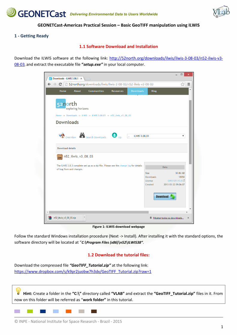
© INPE - National Institute for Space Research - Brazil - 2015 1 GEONETCast-Americas Practical Session – Basic GeoTIFF manipulation using ILWIS 1 - Getting Ready 1.1 Software Download and Installation Download the ILWIS software at the following link: http://52north.org/downloads/ilwis/ilwis-3-08-03/n52-ilwis-v3- 08-03, and extract the executable file “setup.exe” in your local computer. Figure 1: ILWIS download webpage Follow the standard Windows installation procedure (Next -> Install). After installing it with the standard options, the software directory will be located at “C:\Program Files (x86)\n52\ILWIS38”. 1.2 Download the tutorial files: Download the compressed file “GeoTIFF_Tutorial.zip” at the following link: https://www.dropbox.com/s/k9pr2juobw7h3dx/GeoTIFF_Tutorial.zip?raw=1 Hint: Create a folder in the “C:\” directory called “VLAB” and extract the “GeoTIFF_Tutorial.zip” files in it. From now on this folder will be referred as “work folder” in this tutorial.
Transcript of GEONETCast-Americas Practical Session Basic GeoTIFF ... - ILWIS (UNESP - SBMET...Jun 01, 2015 ·...
© INPE - National Institute for Space Research - Brazil - 2015 1
GEONETCast-Americas Practical Session – Basic GeoTIFF manipulation using ILWIS
1 - Getting Ready
1.1 Software Download and Installation
Download the ILWIS software at the following link: http://52north.org/downloads/ilwis/ilwis-3-08-03/n52-ilwis-v3-
08-03, and extract the executable file “setup.exe” in your local computer.
Figure 1: ILWIS download webpage
Follow the standard Windows installation procedure (Next -> Install). After installing it with the standard options, the
software directory will be located at “C:\Program Files (x86)\n52\ILWIS38”.
1.2 Download the tutorial files:
Download the compressed file “GeoTIFF_Tutorial.zip” at the following link:
https://www.dropbox.com/s/k9pr2juobw7h3dx/GeoTIFF_Tutorial.zip?raw=1
Hint: Create a folder in the “C:\” directory called “VLAB” and extract the “GeoTIFF_Tutorial.zip” files in it. From
now on this folder will be referred as “work folder” in this tutorial.
© INPE - National Institute for Space Research - Brazil - 2015 2
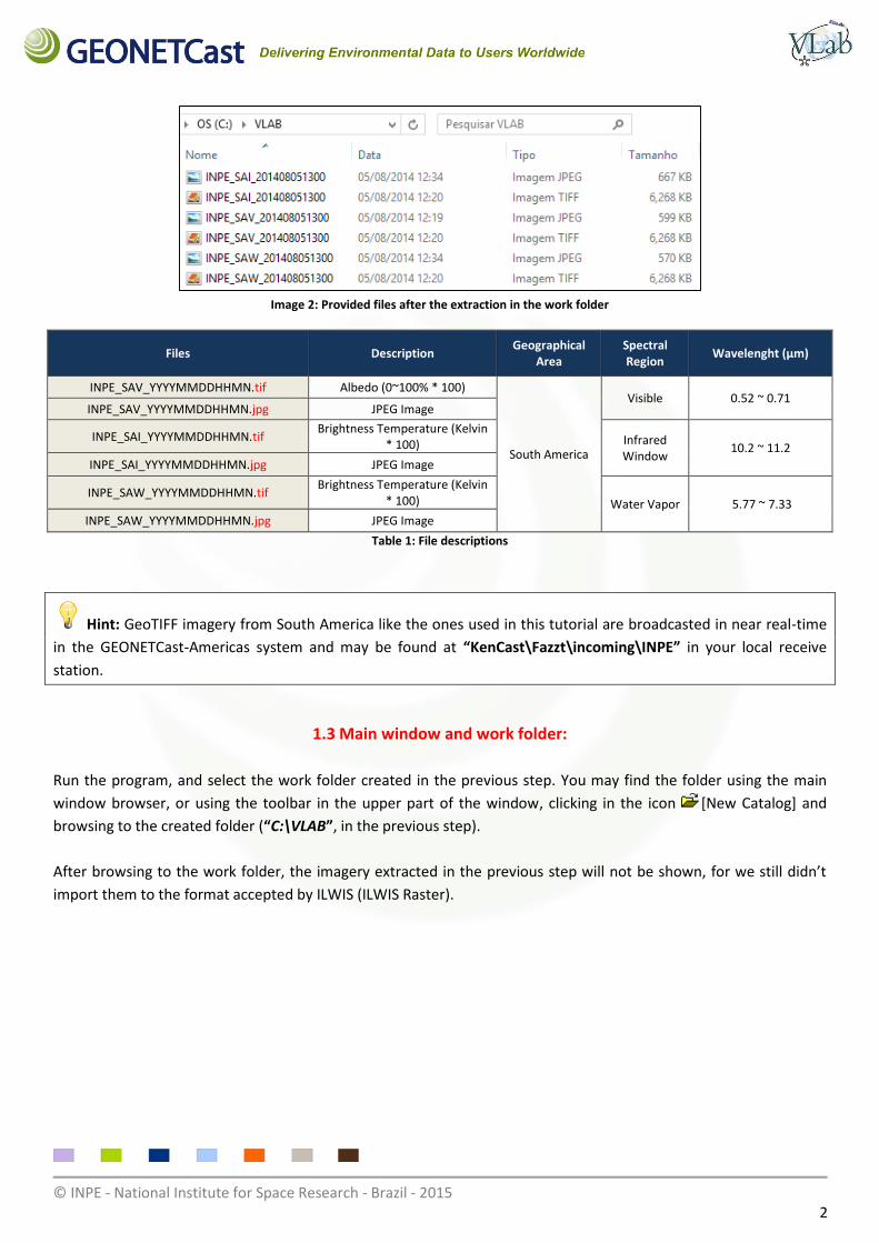
Image 2: Provided files after the extraction in the work folder
Files Description Geographical
Area Spectral Region
Wavelenght (µm)
INPE_SAV_YYYYMMDDHHMN.tif Albedo (0~100% * 100)
South America
Visible 0.52 ~ 0.71 INPE_SAV_YYYYMMDDHHMN.jpg JPEG Image
INPE_SAI_YYYYMMDDHHMN.tif Brightness Temperature (Kelvin
* 100) Infrared Window
10.2 ~ 11.2
INPE_SAI_YYYYMMDDHHMN.jpg JPEG Image
INPE_SAW_YYYYMMDDHHMN.tif Brightness Temperature (Kelvin
* 100) Water Vapor 5.77 ~ 7.33 INPE_SAW_YYYYMMDDHHMN.jpg JPEG Image
Table 1: File descriptions
Hint: GeoTIFF imagery from South America like the ones used in this tutorial are broadcasted in near real-time
in the GEONETCast-Americas system and may be found at “KenCast\Fazzt\incoming\INPE” in your local receive
station.
1.3 Main window and work folder:
Run the program, and select the work folder created in the previous step. You may find the folder using the main
window browser, or using the toolbar in the upper part of the window, clicking in the icon [New Catalog] and
browsing to the created folder (“C:\VLAB”, in the previous step).
After browsing to the work folder, the imagery extracted in the previous step will not be shown, for we still didn’t
import them to the format accepted by ILWIS (ILWIS Raster).
© INPE - National Institute for Space Research - Brazil - 2015 3
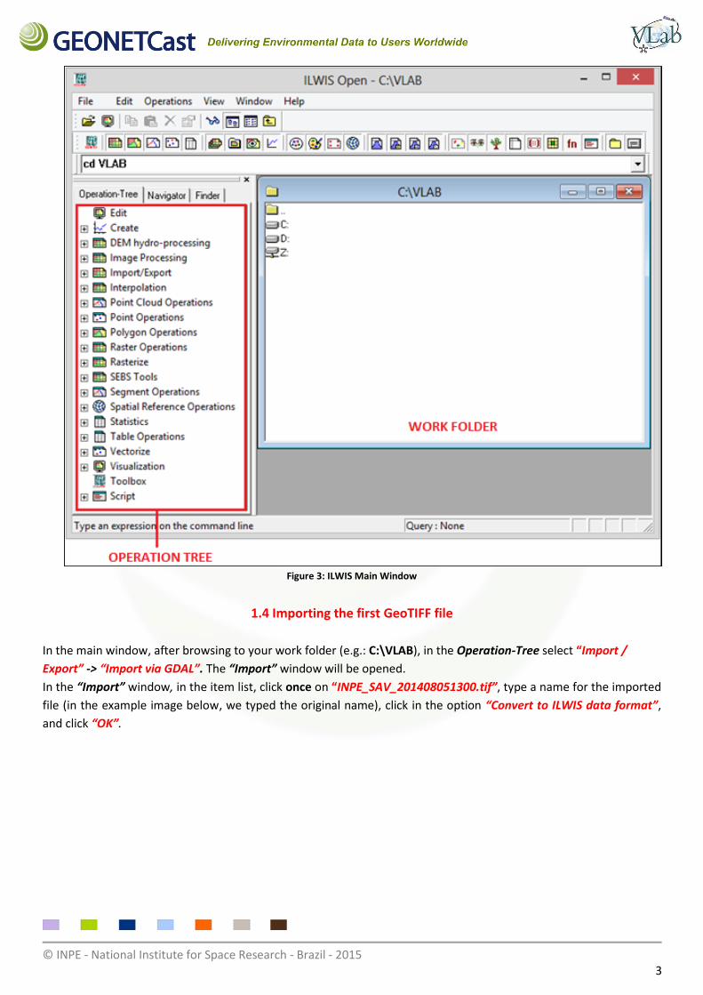
Figure 3: ILWIS Main Window
1.4 Importing the first GeoTIFF file
In the main window, after browsing to your work folder (e.g.: C:\VLAB), in the Operation-Tree select “Import /
Export” -> “Import via GDAL”. The “Import” window will be opened.
In the “Import” window, in the item list, click once on “INPE_SAV_201408051300.tif”, type a name for the imported
file (in the example image below, we typed the original name), click in the option “Convert to ILWIS data format”,
and click “OK”.
© INPE - National Institute for Space Research - Brazil - 2015 4
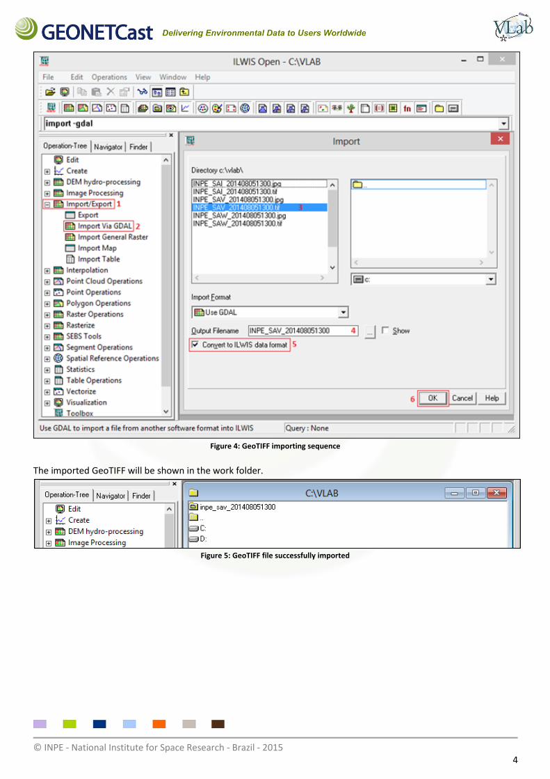
Figure 4: GeoTIFF importing sequence
The imported GeoTIFF will be shown in the work folder.
Figure 5: GeoTIFF file successfully imported
© INPE - National Institute for Space Research - Brazil - 2015 5
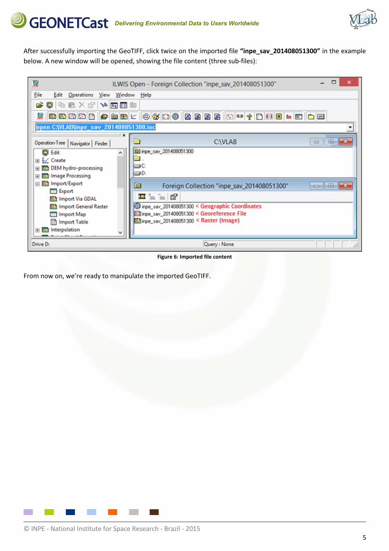
After successfully importing the GeoTIFF, click twice on the imported file “inpe_sav_201408051300” in the example
below. A new window will be opened, showing the file content (three sub-files):
Figure 6: Imported file content
From now on, we’re ready to manipulate the imported GeoTIFF.
© INPE - National Institute for Space Research - Brazil - 2015 6
2 – Manipulating the GeoTIFF’s
Lesson 1 - Analyzing the properties of an image before opening it
2.1 The Geographic Coordinate File
Before starting the manipulation, let’s briefly check some of the imported GeoTIFF image attributes. This is very
important to know when mosaicking, for example.
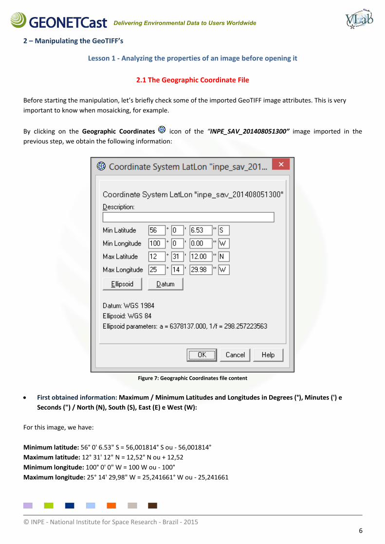
By clicking on the Geographic Coordinates icon of the “INPE_SAV_201408051300” image imported in the
previous step, we obtain the following information:
Figure 7: Geographic Coordinates file content
First obtained information: Maximum / Minimum Latitudes and Longitudes in Degrees (°), Minutes (') e
Seconds (") / North (N), South (S), East (E) e West (W):
For this image, we have:
Minimum latitude: 56° 0' 6.53" S = 56,001814° S ou - 56,001814°
Maximum latitude: 12° 31' 12" N = 12,52° N ou + 12,52
Minimum longitude: 100° 0' 0" W = 100 W ou - 100°
Maximum longitude: 25° 14' 29,98" W = 25,241661° W ou - 25,241661
© INPE - National Institute for Space Research - Brazil - 2015 7
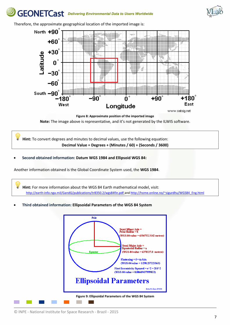
Therefore, the approximate geographical location of the imported image is:
Figure 8: Approximate position of the imported image
Note: The image above is representative, and it’s not generated by the ILWIS software.
Hint: To convert degrees and minutes to decimal values, use the following equation:
Decimal Value = Degrees + (Minutes / 60) + (Seconds / 3600)
Second obtained information: Datum WGS 1984 and Ellipsoid WGS 84:
Another information obtained is the Global Coordinate System used, the WGS 1984.
Hint: For more information about the WGS 84 Earth mathematical model, visit: http://earth-info.nga.mil/GandG/publications/tr8350.2/wgs84fin.pdf and http://home.online.no/~sigurdhu/WGS84_Eng.html
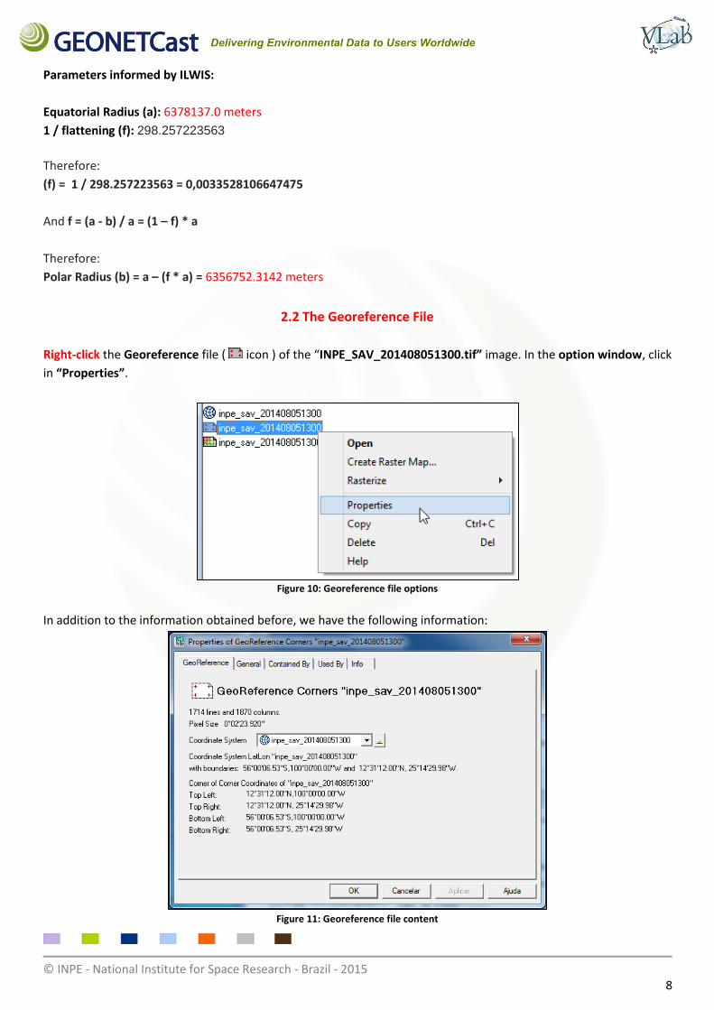
Third obtained information: Ellipsoidal Parameters of the WGS 84 System
Figure 9: Ellipsoidal Parameters of the WGS 84 System
© INPE - National Institute for Space Research - Brazil - 2015 8
Parameters informed by ILWIS:
Equatorial Radius (a): 6378137.0 meters
1 / flattening (f): 298.257223563
Therefore:
(f) = 1 / 298.257223563 = 0,0033528106647475
And f = (a - b) / a = (1 – f) * a
Therefore:
Polar Radius (b) = a – (f * a) = 6356752.3142 meters
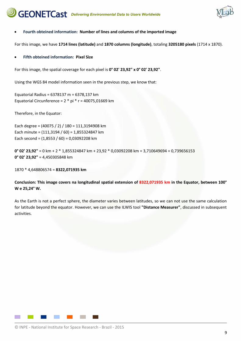
2.2 The Georeference File
Right-click the Georeference file ( icon ) of the “INPE_SAV_201408051300.tif” image. In the option window, click
in “Properties”.
Figure 10: Georeference file options
In addition to the information obtained before, we have the following information:
Figure 11: Georeference file content
© INPE - National Institute for Space Research - Brazil - 2015 9
Fourth obteined information: Number of lines and columns of the imported image
For this image, we have 1714 lines (latitude) and 1870 columns (longitude), totaling 3205180 pixels (1714 x 1870).
Fifth obteined information: Pixel Size
For this image, the spatial coverage for each pixel is 0° 02' 23,92" x 0° 02' 23,92".
Using the WGS 84 model information seen in the previous step, we know that:
Equatorial Radius = 6378137 m = 6378,137 km
Equatorial Circunference = 2 * pi * r = 40075,01669 km
Therefore, in the Equator:
Each degree = (40075 / 2) / 180 = 111,3194908 km
Each minute = (111,3194 / 60) = 1,855324847 km
Each second = (1,8553 / 60) = 0,03092208 km
0° 02' 23,92" = 0 km + 2 * 1,855324847 km + 23,92 * 0,03092208 km = 3,710649694 + 0,739656153
0° 02' 23,92" = 4,450305848 km
1870 * 4,648806574 = 8322,071935 km
Conclusion: This image covers na longitudinal spatial extension of 8322,071935 km in the Equator, between 100°
W e 25,24° W.
As the Earth is not a perfect sphere, the diameter varies between latitudes, so we can not use the same calculation
for latitude beyond the equator. However, we can use the ILWIS tool "Distance Measurer", discussed in subsequent
activities.
© INPE - National Institute for Space Research - Brazil - 2015 10
Lesson 2 – Extracting physical information from each pixel
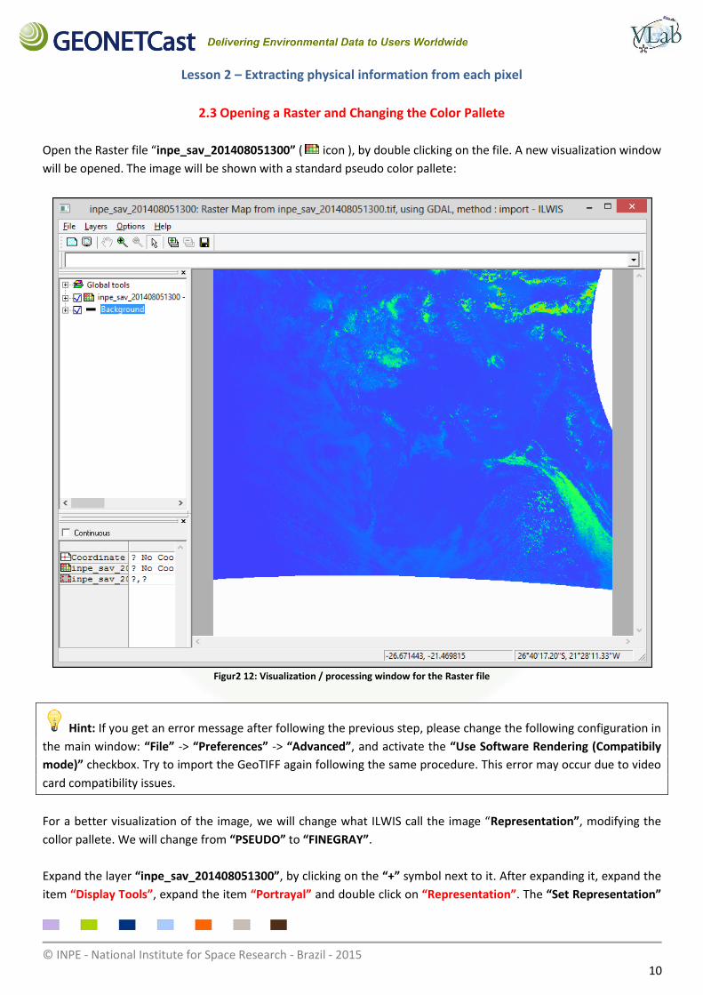
2.3 Opening a Raster and Changing the Color Pallete
Open the Raster file “inpe_sav_201408051300” ( icon ), by double clicking on the file. A new visualization window
will be opened. The image will be shown with a standard pseudo color pallete:
Figur2 12: Visualization / processing window for the Raster file
Hint: If you get an error message after following the previous step, please change the following configuration in
the main window: “File” -> “Preferences” -> “Advanced”, and activate the “Use Software Rendering (Compatibily
mode)” checkbox. Try to import the GeoTIFF again following the same procedure. This error may occur due to video
card compatibility issues.
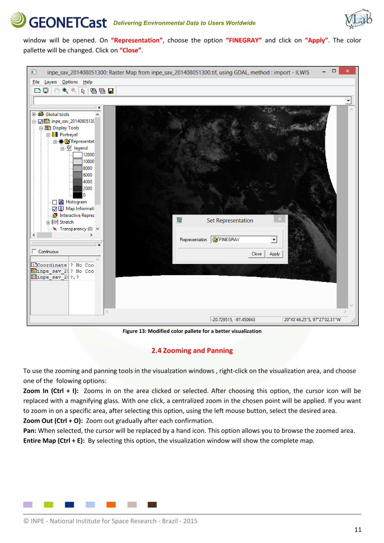
For a better visualization of the image, we will change what ILWIS call the image “Representation”, modifying the
collor pallete. We will change from “PSEUDO” to “FINEGRAY”.
Expand the layer “inpe_sav_201408051300”, by clicking on the “+” symbol next to it. After expanding it, expand the
item “Display Tools”, expand the item “Portrayal” and double click on “Representation”. The “Set Representation”
© INPE - National Institute for Space Research - Brazil - 2015 11
window will be opened. On “Representation”, choose the option “FINEGRAY” and click on “Apply”. The color
pallette will be changed. Click on “Close”.
Figure 13: Modified color pallete for a better visualization
2.4 Zooming and Panning
To use the zooming and panning tools in the visualzation windows , right-click on the visualization area, and choose
one of the folowing options:
Zoom In (Ctrl + I): Zooms in on the area clicked or selected. After choosing this option, the cursor icon will be
replaced with a magnifying glass. With one click, a centralized zoom in the chosen point will be applied. If you want
to zoom in on a specific area, after selecting this option, using the left mouse button, select the desired area.
Zoom Out (Ctrl + O): Zoom out gradually after each confirmation.
Pan: When selected, the cursor will be replaced by a hand icon. This option allows you to browse the zoomed area.
Entire Map (Ctrl + E): By selecting this option, the visualization window will show the complete map.
© INPE - National Institute for Space Research - Brazil - 2015 12
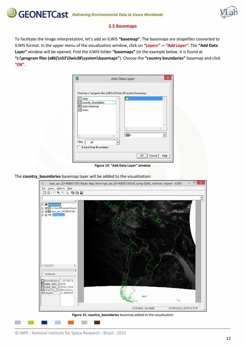
2.5 Basemaps
To facilitate the image interpretation, let’s add an ILWIS “basemap”. The basemaps are shapefiles converted to
ILWIS format. In the upper menu of the visualization window, click on “Layers” -> “Add Layer”. The “Add Data
Layer” window will be opened. Find the ILWIS folder “basemaps” (in the example below, it is found at
“c:\program files (x86)\n52\ilwis38\system\basemaps”). Choose the “country boundaries” basemap and click
“OK”.
Figure 14: “Add Data Layer” window
The country_boundaries basemap layer will be added to the visualization:
Figure 15: country_boundaries basemap added to the visualization
© INPE - National Institute for Space Research - Brazil - 2015 13
Hint: To import your own custom shapefile (.shp), in ILWIS main window (not the visualization window), go to
“File” -> “Import” -> expand the “Geospatial Data Absraction Library (GDAL)” option -> expand the “vector” option
-> and choose “ESRI Shapefile”. Browse the input file and click “OK”. A new raster will be created. Import the
created raster into our visualization window following the previous steps.
Now we have four layers in our visualization window, being:
- Global Tools;
- country_boundaries (which we just added);
- inpe_sav_201406261200 (the image);
- Background (background visualization configuration).
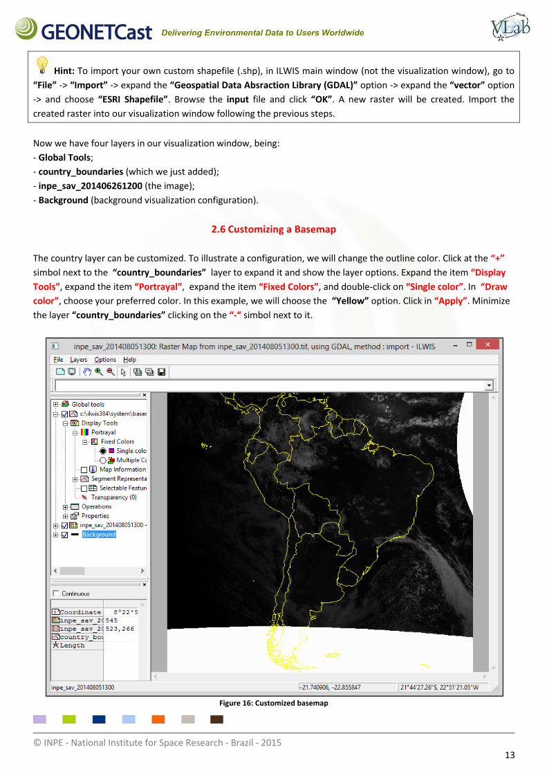
2.6 Customizing a Basemap
The country layer can be customized. To illustrate a configuration, we will change the outline color. Click at the “+”
simbol next to the “country_boundaries” layer to expand it and show the layer options. Expand the item “Display
Tools”, expand the item “Portrayal”, expand the item “Fixed Colors”, and double-click on “Single color”. In “Draw
color”, choose your preferred color. In this example, we will choose the “Yellow” option. Click in “Apply”. Minimize
the layer “country_boundaries” clicking on the “-“ simbol next to it.
Figure 16: Customized basemap
© INPE - National Institute for Space Research - Brazil - 2015 14
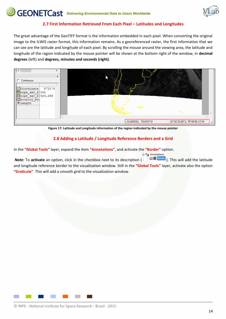
2.7 First Information Retrieved From Each Pixel – Latitudes and Longitudes
The great advantage of the GeoTIFF format is the information embedded in each pixel. When converting the original
image to the ILWIS raster format, this information remains. As a georeferenced raster, the first information that we
can see are the latitude and longitude of each pixel. By scrolling the mouse around the viewing area, the latitude and
longitude of the ragion indicated by the mouse pointer will be shown at the bottom right of the window, in decimal
degrees (left) and degrees, minutes and seconds (right).
Figure 17: Latitude and Longitude information of the region indicated by the mouse pointer
2.8 Adding a Latitude / Longitude Reference Borders and a Grid
In the “Global Tools” layer, expand the item “Annotations”, and activate the “Border” option.
Note: To activate an option, click in the checkbox next to its description ( ). This will add the latitude
and longitude reference border to the visualization window. Still in the “Global Tools” layer, activate also the option
“Graticule”. This will add a smooth grid to the visualization window.
© INPE - National Institute for Space Research - Brazil - 2015 15
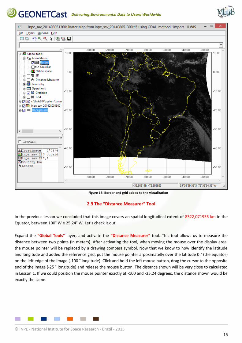
Figure 18: Border and grid added to the visualization
2.9 The “Distance Measurer” Tool
In the previous lesson we concluded that this image covers an spatial longitudinal extent of 8322,071935 km in the
Equator, between 100° W e 25,24° W. Let’s check it out.
Expand the “Global Tools” layer, and activate the “Distance Measurer” tool. This tool allows us to measure the
distance between two points (in meters). After activating the tool, when moving the mouse over the display area,
the mouse pointer will be replaced by a drawing compass symbol. Now that we know to how identify the latitude
and longitude and added the reference grid, put the mouse pointer arpoximatelly over the latitude 0 ° (the equator)
on the left edge of the image (-100 ° longitude). Click and hold the left mouse button, drag the cursor to the opposite
end of the image (-25 ° longitude) and release the mouse button. The distance shown will be very close to calculated
in Lesson 1. If we could position the mouse pointer exactly at -100 and -25.24 degrees, the distance shown would be
exactly the same.
© INPE - National Institute for Space Research - Brazil - 2015 16
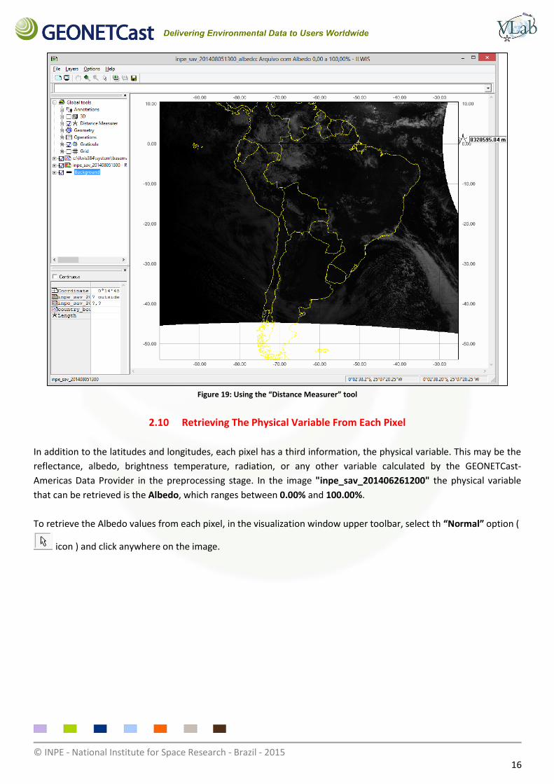
Figure 19: Using the “Distance Measurer” tool
2.10 Retrieving The Physical Variable From Each Pixel
In addition to the latitudes and longitudes, each pixel has a third information, the physical variable. This may be the
reflectance, albedo, brightness temperature, radiation, or any other variable calculated by the GEONETCast-
Americas Data Provider in the preprocessing stage. In the image "inpe_sav_201406261200" the physical variable
that can be retrieved is the Albedo, which ranges between 0.00% and 100.00%.
To retrieve the Albedo values from each pixel, in the visualization window upper toolbar, select th “Normal” option (
icon ) and click anywhere on the image.
© INPE - National Institute for Space Research - Brazil - 2015 17
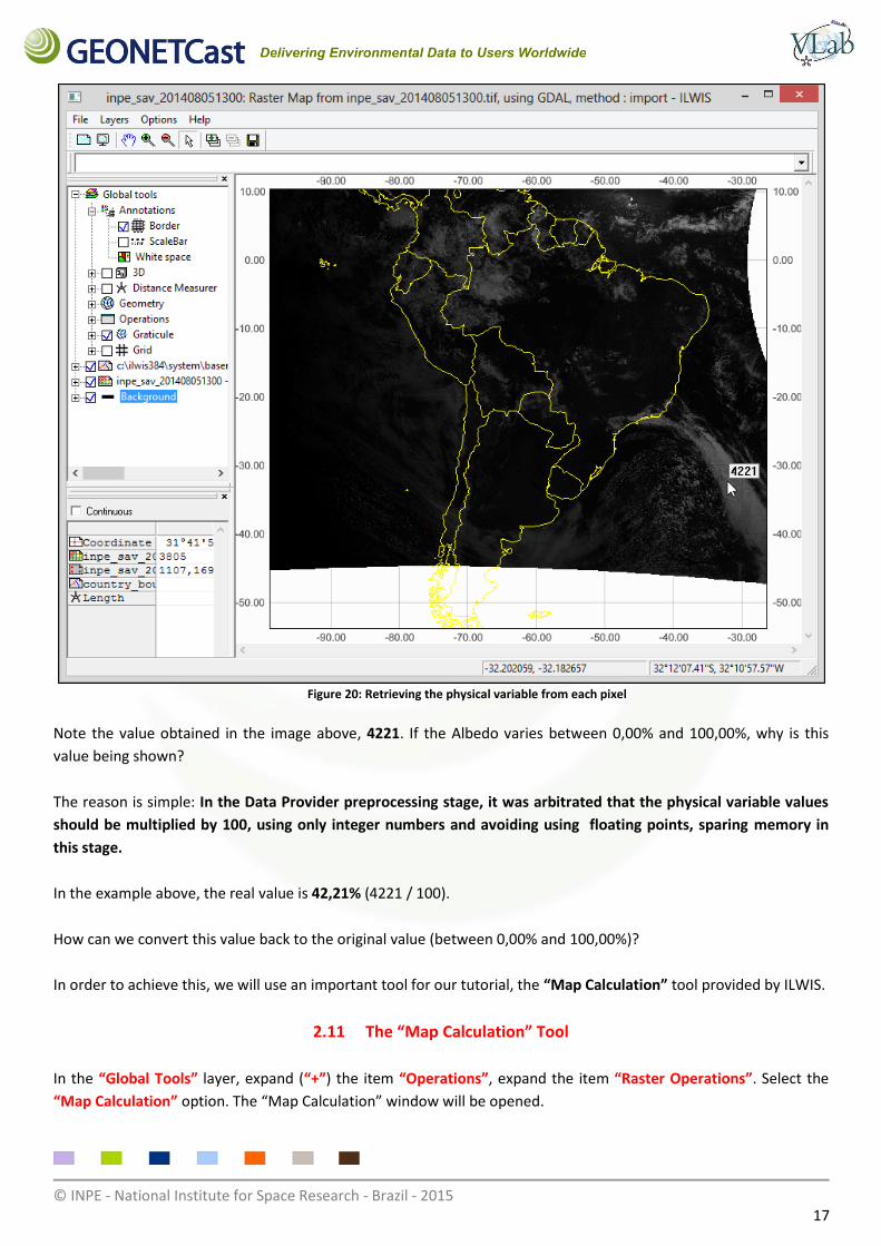
Figure 20: Retrieving the physical variable from each pixel
Note the value obtained in the image above, 4221. If the Albedo varies between 0,00% and 100,00%, why is this
value being shown?
The reason is simple: In the Data Provider preprocessing stage, it was arbitrated that the physical variable values
should be multiplied by 100, using only integer numbers and avoiding using floating points, sparing memory in
this stage.
In the example above, the real value is 42,21% (4221 / 100).
How can we convert this value back to the original value (between 0,00% and 100,00%)?
In order to achieve this, we will use an important tool for our tutorial, the “Map Calculation” tool provided by ILWIS.
2.11 The “Map Calculation” Tool
In the “Global Tools” layer, expand (“+”) the item “Operations”, expand the item “Raster Operations”. Select the
“Map Calculation” option. The “Map Calculation” window will be opened.
© INPE - National Institute for Space Research - Brazil - 2015 18
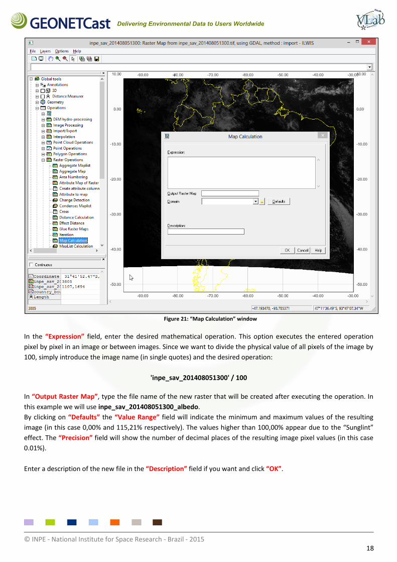
Figure 21: “Map Calculation” window
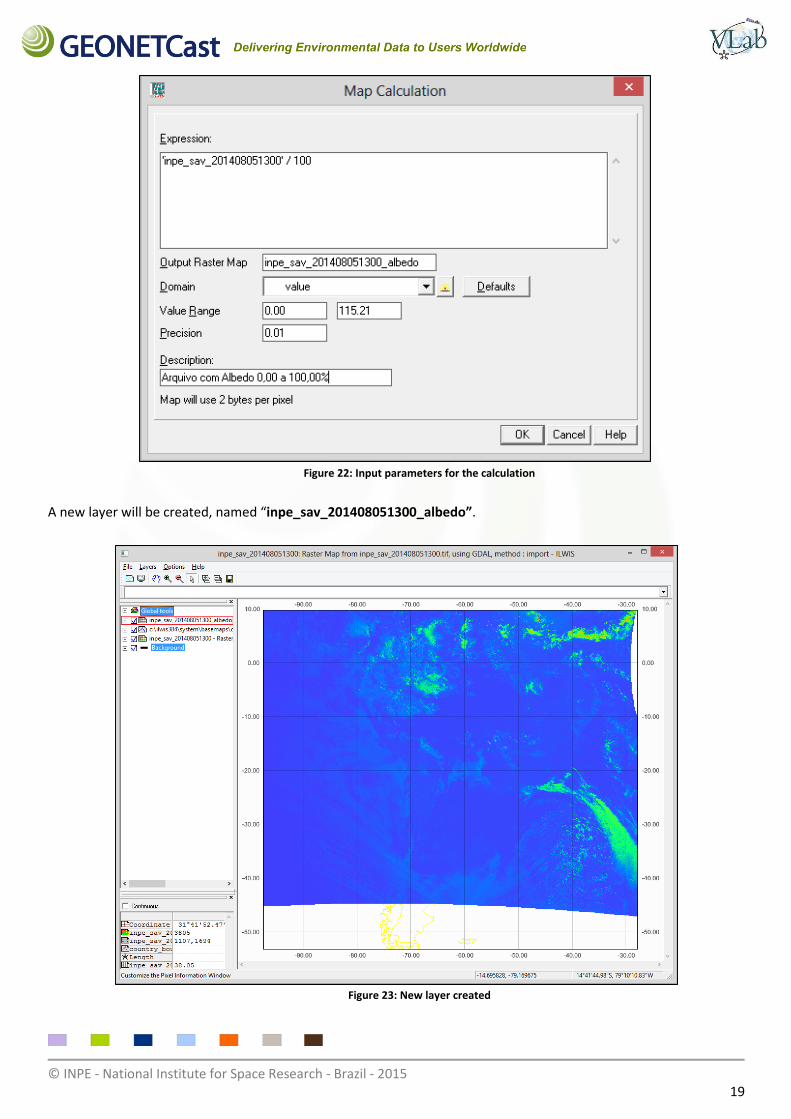
In the “Expression” field, enter the desired mathematical operation. This option executes the entered operation
pixel by pixel in an image or between images. Since we want to divide the physical value of all pixels of the image by
100, simply introduce the image name (in single quotes) and the desired operation:
'inpe_sav_201408051300' / 100
In “Output Raster Map”, type the file name of the new raster that will be created after executing the operation. In
this example we will use inpe_sav_201408051300_albedo.
By clicking on “Defaults” the “Value Range” field will indicate the minimum and maximum values of the resulting
image (in this case 0,00% and 115,21% respectively). The values higher than 100,00% appear due to the “Sunglint”
effect. The “Precision” field will show the number of decimal places of the resulting image pixel values (in this case
0.01%).
Enter a description of the new file in the “Description” field if you want and click “OK”.
© INPE - National Institute for Space Research - Brazil - 2015 19
Figure 22: Input parameters for the calculation
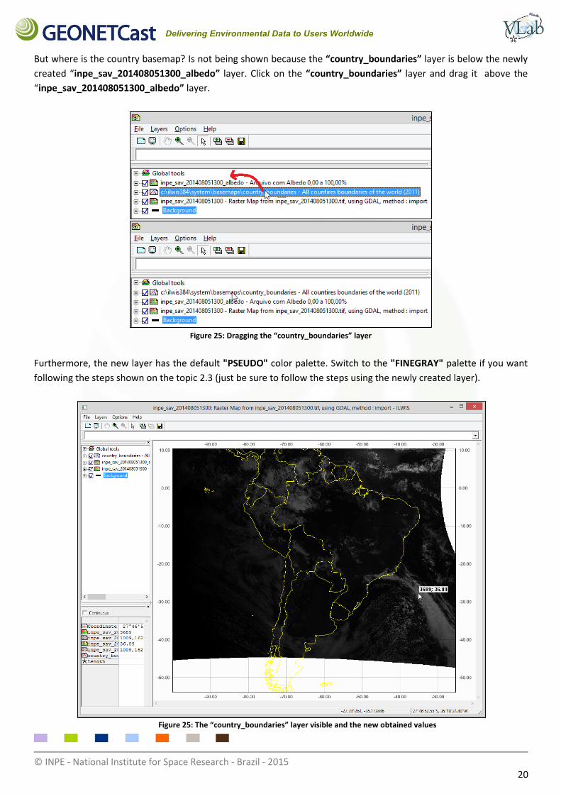
A new layer will be created, named “inpe_sav_201408051300_albedo”.
Figure 23: New layer created
© INPE - National Institute for Space Research - Brazil - 2015 20
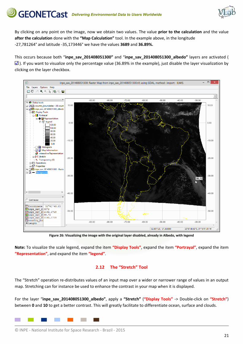
But where is the country basemap? Is not being shown because the “country_boundaries” layer is below the newly
created “inpe_sav_201408051300_albedo” layer. Click on the “country_boundaries” layer and drag it above the
“inpe_sav_201408051300_albedo” layer.
Figure 25: Dragging the “country_boundaries” layer
Furthermore, the new layer has the default "PSEUDO" color palette. Switch to the "FINEGRAY" palette if you want
following the steps shown on the topic 2.3 (just be sure to follow the steps using the newly created layer).
Figure 25: The “country_boundaries” layer visible and the new obtained values
© INPE - National Institute for Space Research - Brazil - 2015 21
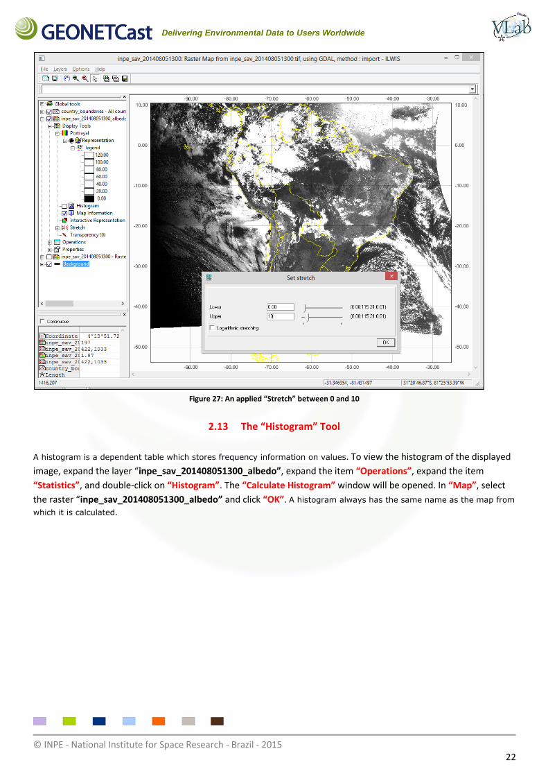
By clicking on any point on the image, now we obtain two values. The value prior to the calculation and the value
after the calculation done with the “Map Calculation” tool. In the example above, in the longitude
-27,781264° and latitude -35,173446° we have the values 3689 and 36.89%.
This occurs because both “inpe_sav_201408051300” and “inpe_sav_201408051300_albedo” layers are activated (
). If you want to visualize only the percentage value (36.89% in the example), just disable the layer visualization by
clicking on the layer checkbox.
Figure 26: Visualizing the image with the original layer disabled, already in Albedo, with legend
Note: To visualize the scale legend, expand the item “Display Tools”, expand the item “Portrayal”, expand the item
“Representation”, and expand the item “legend”.
2.12 The “Stretch” Tool
The “Stretch” operation re-distributes values of an input map over a wider or narrower range of values in an output
map. Stretching can for instance be used to enhance the contrast in your map when it is displayed.
For the layer “inpe_sav_201408051300_albedo”, apply a “Stretch” (“Display Tools” -> Double-click on “Stretch”)
between 0 and 10 to get a better contrast. This will greatly facilitate to differentiate ocean, surface and clouds.
© INPE - National Institute for Space Research - Brazil - 2015 22
Figure 27: An applied “Stretch” between 0 and 10
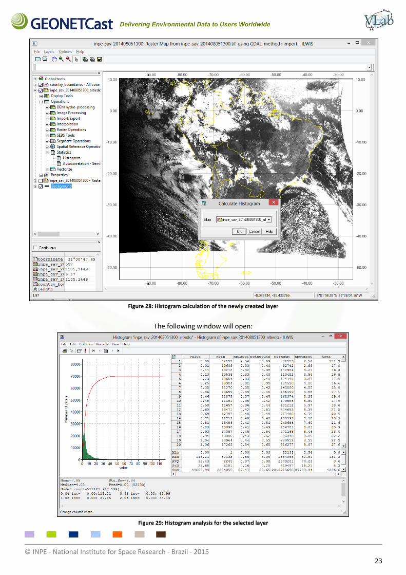
2.13 The “Histogram” Tool
A histogram is a dependent table which stores frequency information on values. To view the histogram of the displayed
image, expand the layer “inpe_sav_201408051300_albedo”, expand the item “Operations”, expand the item
“Statistics”, and double-click on “Histogram”. The “Calculate Histogram” window will be opened. In “Map”, select
the raster “inpe_sav_201408051300_albedo” and click “OK”. A histogram always has the same name as the map from
which it is calculated.
© INPE - National Institute for Space Research - Brazil - 2015 23
Figure 28: Histogram calculation of the newly created layer
The following window will open:
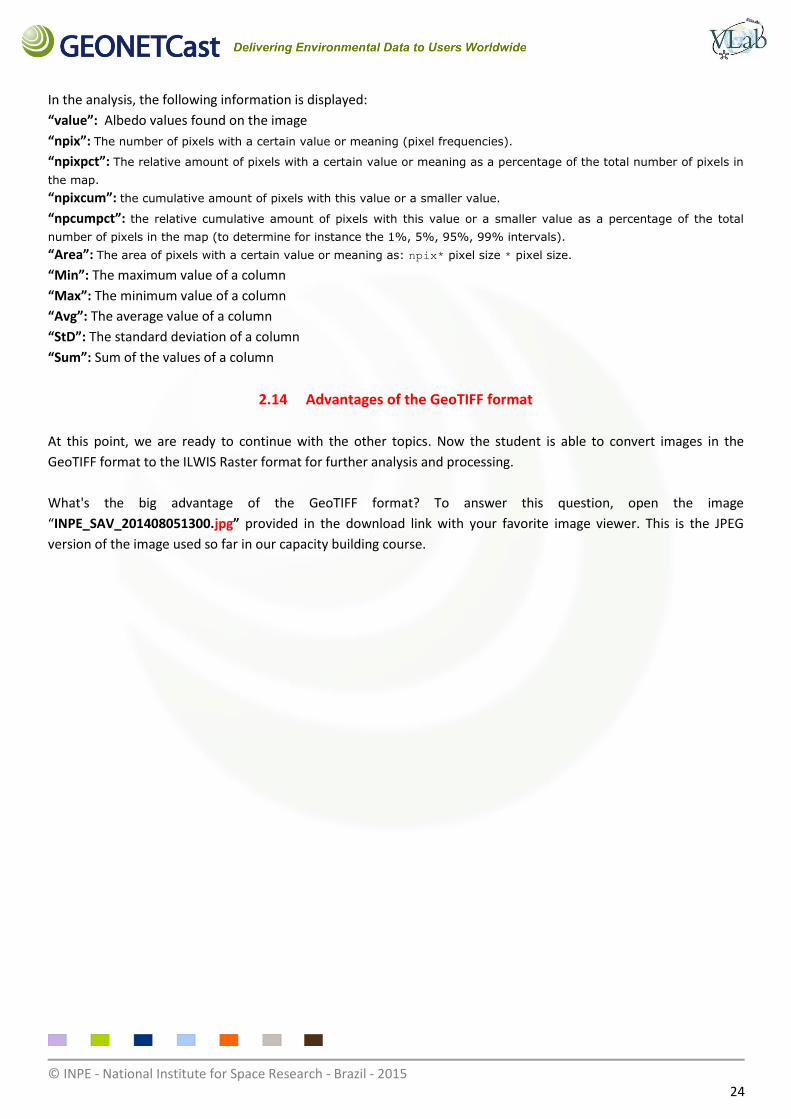
Figure 29: Histogram analysis for the selected layer
© INPE - National Institute for Space Research - Brazil - 2015 24
In the analysis, the following information is displayed:
“value”: Albedo values found on the image
“npix”: The number of pixels with a certain value or meaning (pixel frequencies).
“npixpct”: The relative amount of pixels with a certain value or meaning as a percentage of the total number of pixels in
the map. “npixcum”: the cumulative amount of pixels with this value or a smaller value.
“npcumpct”: the relative cumulative amount of pixels with this value or a smaller value as a percentage of the total
number of pixels in the map (to determine for instance the 1%, 5%, 95%, 99% intervals). “Area”: The area of pixels with a certain value or meaning as: npix* pixel size * pixel size.
“Min”: The maximum value of a column
“Max”: The minimum value of a column
“Avg”: The average value of a column
“StD”: The standard deviation of a column
“Sum”: Sum of the values of a column
2.14 Advantages of the GeoTIFF format
At this point, we are ready to continue with the other topics. Now the student is able to convert images in the
GeoTIFF format to the ILWIS Raster format for further analysis and processing.
What's the big advantage of the GeoTIFF format? To answer this question, open the image
“INPE_SAV_201408051300.jpg” provided in the download link with your favorite image viewer. This is the JPEG
version of the image used so far in our capacity building course.
© INPE - National Institute for Space Research - Brazil - 2015 25
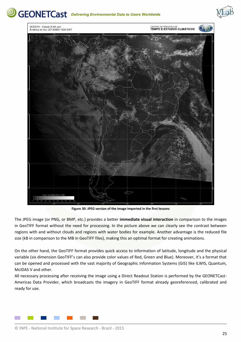
Figure 30: JPEG version of the image imported in the first lessons
The JPEG image (or PNG, or BMP, etc.) provides a better immediate visual interaction in comparison to the images
in GeoTIFF format without the need for processing. In the picture above we can clearly see the contrast between
regions with and without clouds and regions with water bodies for example. Another advantage is the reduced file
size (kB in comparison to the MB in GeoTIFF files), making this an optimal format for creating animations.
On the other hand, the GeoTIFF format provides quick access to information of latitude, longitude and the physical
variable (six dimension GeoTIFF’s can also provide color values of Red, Green and Blue). Moreover, it’s a format that
can be opened and processed with the vast majority of Geographic Information Systems (GIS) like ILWIS, Quantum,
McIDAS V and other.
All necessary processing after receiving the image using a Direct Readout Station is performed by the GEONETCast-
Americas Data Provider, which broadcasts the imagery in GeoTIFF format already georeferenced, calibrated and
ready for use.
© INPE - National Institute for Space Research - Brazil - 2015 26
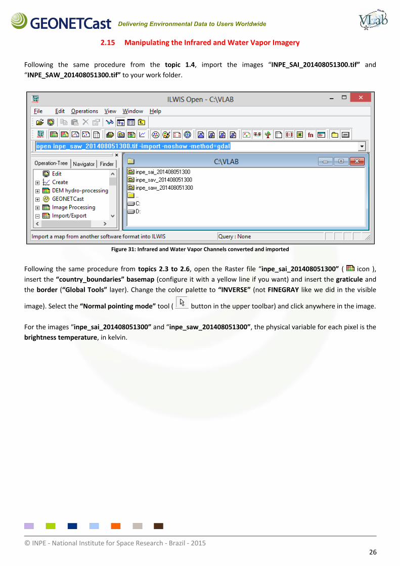
2.15 Manipulating the Infrared and Water Vapor Imagery
Following the same procedure from the topic 1.4, import the images “INPE_SAI_201408051300.tif” and
“INPE_SAW_201408051300.tif” to your work folder.
Figure 31: Infrared and Water Vapor Channels converted and imported
Following the same procedure from topics 2.3 to 2.6, open the Raster file “inpe_sai_201408051300” ( icon ),
insert the “country_boundaries” basemap (configure it with a yellow line if you want) and insert the graticule and
the border (“Global Tools” layer). Change the color palette to “INVERSE” (not FINEGRAY like we did in the visible
image). Select the “Normal pointing mode” tool ( button in the upper toolbar) and click anywhere in the image.
For the images “inpe_sai_201408051300” and “inpe_saw_201408051300”, the physical variable for each pixel is the
brightness temperature, in kelvin.
© INPE - National Institute for Space Research - Brazil - 2015 27
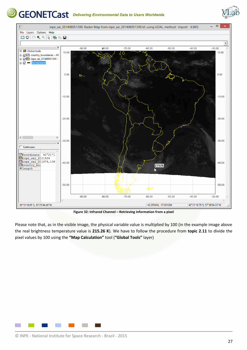
Figure 32: Infrared Channel – Retrieving information from a pixel
Please note that, as in the visible image, the physical variable value is multiplied by 100 (in the example image above
the real brightness temperature value is 215.26 K). We have to follow the procedure from topic 2.11 to divide the
pixel values by 100 using the “Map Calculation” tool (“Global Tools” layer)

© INPE - National Institute for Space Research - Brazil - 2015 28
Figure 33: Inserted parameters for the division
In “Output Raster Map”, type the file name inpe_sai_201408051300_kelvin. By clicking “Default”, we see that the
minimum and maximum values of the resulting file will be -54,53 K and 309,11 K respectively.
As in topic 2.11, after the calculation, drag the “country_boundaries” layer above the newly
“inpe_sai_201408051300_kelvin”, and disable the “inpe_sai_201408051300” layer to visualize only the value in
Kelvin when clicking in a certain pixel. Change the color palette to “INVERSE”.
© INPE - National Institute for Space Research - Brazil - 2015 29
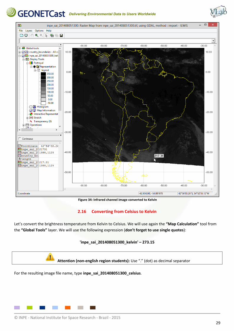
Figure 34: Infrared channel image converted to Kelvin
2.16 Converting from Celsius to Kelvin
Let’s convert the brightness temperature from Kelvin to Celsius. We will use again the “Map Calculation” tool from
the “Global Tools” layer. We will use the following expression (don’t forget to use single quotes):
'inpe_sai_201408051300_kelvin' – 273.15
Attention (non-english region students): Use “.” (dot) as decimal separator
For the resulting image file name, type inpe_sai_201408051300_celsius.
© INPE - National Institute for Space Research - Brazil - 2015 30
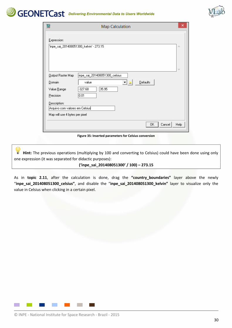
Figure 35: Inserted parameters for Celsius conversion
Hint: The previous operations (multiplying by 100 and converting to Celsius) could have been done using only
one expression (it was separated for didactic purposes):
(‘inpe_sai_201408051300’ / 100) – 273.15
As in topic 2.11, after the calculation is done, drag the “country_boundaries” layer above the newly
“inpe_sai_201408051300_celsius”, and disable the “inpe_sai_201408051300_kelvin” layer to visualize only the
value in Celsius when clicking in a certain pixel.
© INPE - National Institute for Space Research - Brazil - 2015 31
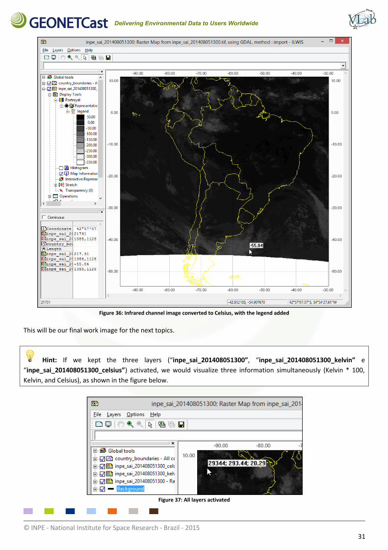
Figure 36: Infrared channel image converted to Celsius, with the legend added
This will be our final work image for the next topics.
Hint: If we kept the three layers (“inpe_sai_201408051300”, “inpe_sai_201408051300_kelvin” e
“inpe_sai_201408051300_celsius”) activated, we would visualize three information simultaneously (Kelvin * 100,
Kelvin, and Celsius), as shown in the figure below.
Figure 37: All layers activated
© INPE - National Institute for Space Research - Brazil - 2015 32
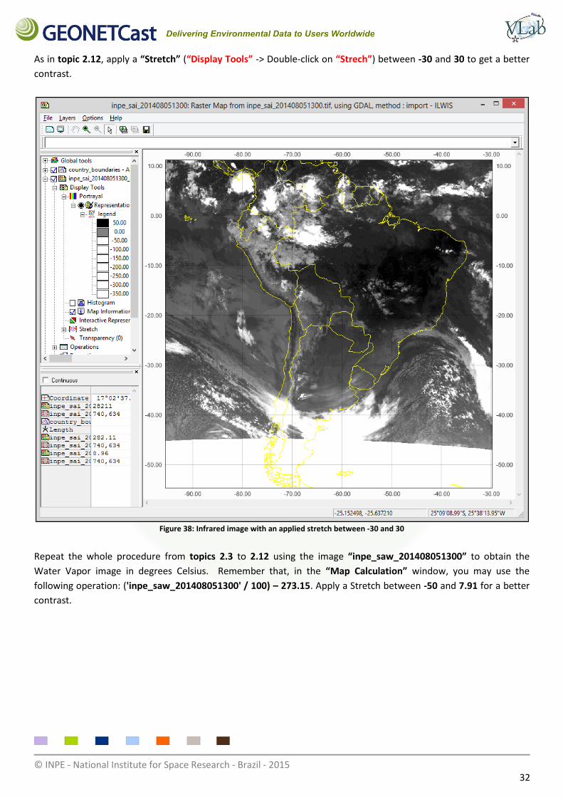
As in topic 2.12, apply a “Stretch” (“Display Tools” -> Double-click on “Strech”) between -30 and 30 to get a better
contrast.
Figure 38: Infrared image with an applied stretch between -30 and 30
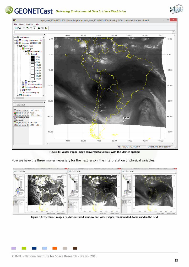
Repeat the whole procedure from topics 2.3 to 2.12 using the image “inpe_saw_201408051300” to obtain the
Water Vapor image in degrees Celsius. Remember that, in the “Map Calculation” window, you may use the
following operation: ('inpe_saw_201408051300' / 100) – 273.15. Apply a Stretch between -50 and 7.91 for a better
contrast.
© INPE - National Institute for Space Research - Brazil - 2015 33
Figure 39: Water Vapor image converted to Celsius, with the Stretch applied
Now we have the three images necessary for the next lesson, the interpretation of physical variables.
Figure 38: The three images (visible, infrared window and water vapor, manipulated, to be used in the next
© INPE - National Institute for Space Research - Brazil - 2015 34
Lesson 3 – Interpretation of physical variables
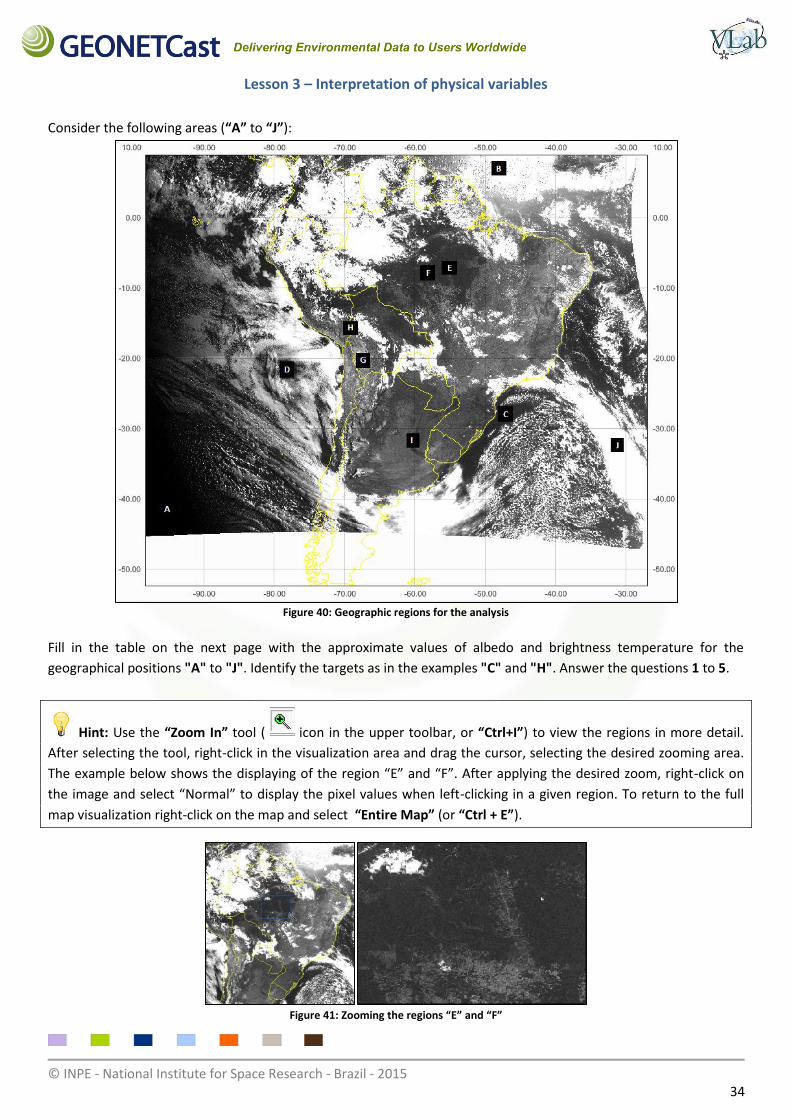
Consider the following areas (“A” to “J”):
Figure 40: Geographic regions for the analysis
Fill in the table on the next page with the approximate values of albedo and brightness temperature for the
geographical positions "A" to "J". Identify the targets as in the examples "C" and "H". Answer the questions 1 to 5.
Hint: Use the “Zoom In” tool ( icon in the upper toolbar, or “Ctrl+I”) to view the regions in more detail.
After selecting the tool, right-click in the visualization area and drag the cursor, selecting the desired zooming area.
The example below shows the displaying of the region “E” and “F”. After applying the desired zoom, right-click on
the image and select “Normal” to display the pixel values when left-clicking in a given region. To return to the full
map visualization right-click on the map and select “Entire Map” (or “Ctrl + E”).
Figure 41: Zooming the regions “E” and “F”
© INPE - National Institute for Space Research - Brazil - 2015 35
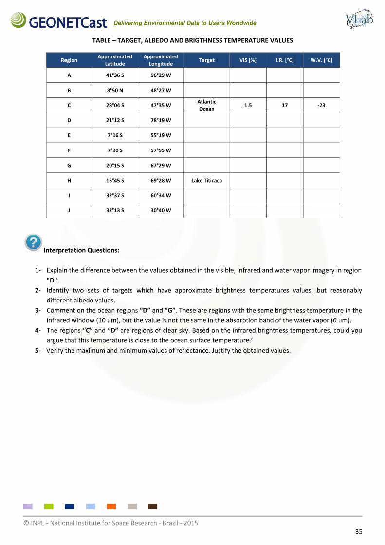
TABLE – TARGET, ALBEDO AND BRIGTHNESS TEMPERATURE VALUES
Region Approximated
Latitude Approximated
Longitude Target VIS [%] I.R. [°C] W.V. [°C]
A 41°36 S 96°29 W
B 8°50 N 48°27 W
C 28°04 S 47°35 W Atlantic Ocean
1.5 17 -23
D 21°12 S 78°19 W
E 7°16 S 55°19 W
F 7°30 S 57°55 W
G 20°15 S 67°29 W
H 15°45 S 69°28 W Lake Titicaca
I 32°37 S 60°34 W
J 32°13 S 30°40 W
Interpretation Questions:
1- Explain the difference between the values obtained in the visible, infrared and water vapor imagery in region
"D".
2- Identify two sets of targets which have approximate brightness temperatures values, but reasonably
different albedo values.
3- Comment on the ocean regions “D” and “G”. These are regions with the same brightness temperature in the
infrared window (10 um), but the value is not the same in the absorption band of the water vapor (6 um).
4- The regions “C” and “D” are regions of clear sky. Based on the infrared brightness temperatures, could you
argue that this temperature is close to the ocean surface temperature?
5- Verify the maximum and minimum values of reflectance. Justify the obtained values.
© INPE - National Institute for Space Research - Brazil - 2015 36
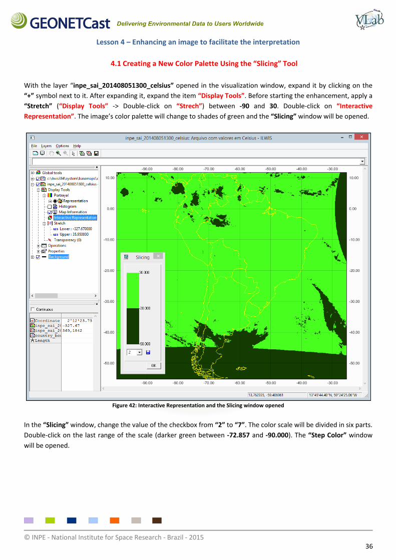
Lesson 4 – Enhancing an image to facilitate the interpretation
4.1 Creating a New Color Palette Using the “Slicing” Tool
With the layer “inpe_sai_201408051300_celsius” opened in the visualization window, expand it by clicking on the
“+” symbol next to it. After expanding it, expand the item “Display Tools”. Before starting the enhancement, apply a
“Stretch” (“Display Tools” -> Double-click on “Strech”) between -90 and 30. Double-click on “Interactive
Representation”. The image’s color palette will change to shades of green and the “Slicing” window will be opened.
Figure 42: Interactive Representation and the Slicing window opened
In the “Slicing” window, change the value of the checkbox from “2” to “7”. The color scale will be divided in six parts.
Double-click on the last range of the scale (darker green between -72.857 and -90.000). The “Step Color” window
will be opened.
© INPE - National Institute for Space Research - Brazil - 2015 37
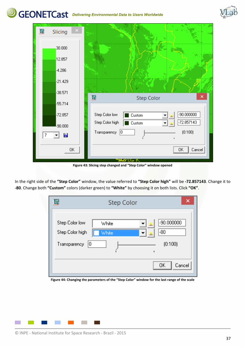
Figure 43: Slicing step changed and “Step Color” window opened
In the right side of the “Step Color” window, the value referred to “Step Color high” will be -72.857143. Change it to
-80. Change both “Custom” colors (darker green) to “White” by choosing it on both lists. Click “OK”.
Figure 44: Changing the parameters of the “Step Color” window for the last range of the scale
© INPE - National Institute for Space Research - Brazil - 2015 38
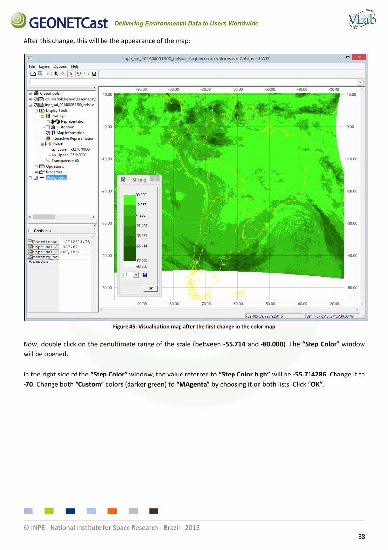
After this change, this will be the appearance of the map:
Figure 45: Visualization map after the first change in the color map
Now, double click on the penultimate range of the scale (between -55.714 and -80.000). The “Step Color” window
will be opened.
In the right side of the “Step Color” window, the value referred to “Step Color high” will be -55.714286. Change it to
-70. Change both “Custom” colors (darker green) to “MAgenta” by choosing it on both lists. Click “OK”.
© INPE - National Institute for Space Research - Brazil - 2015 39
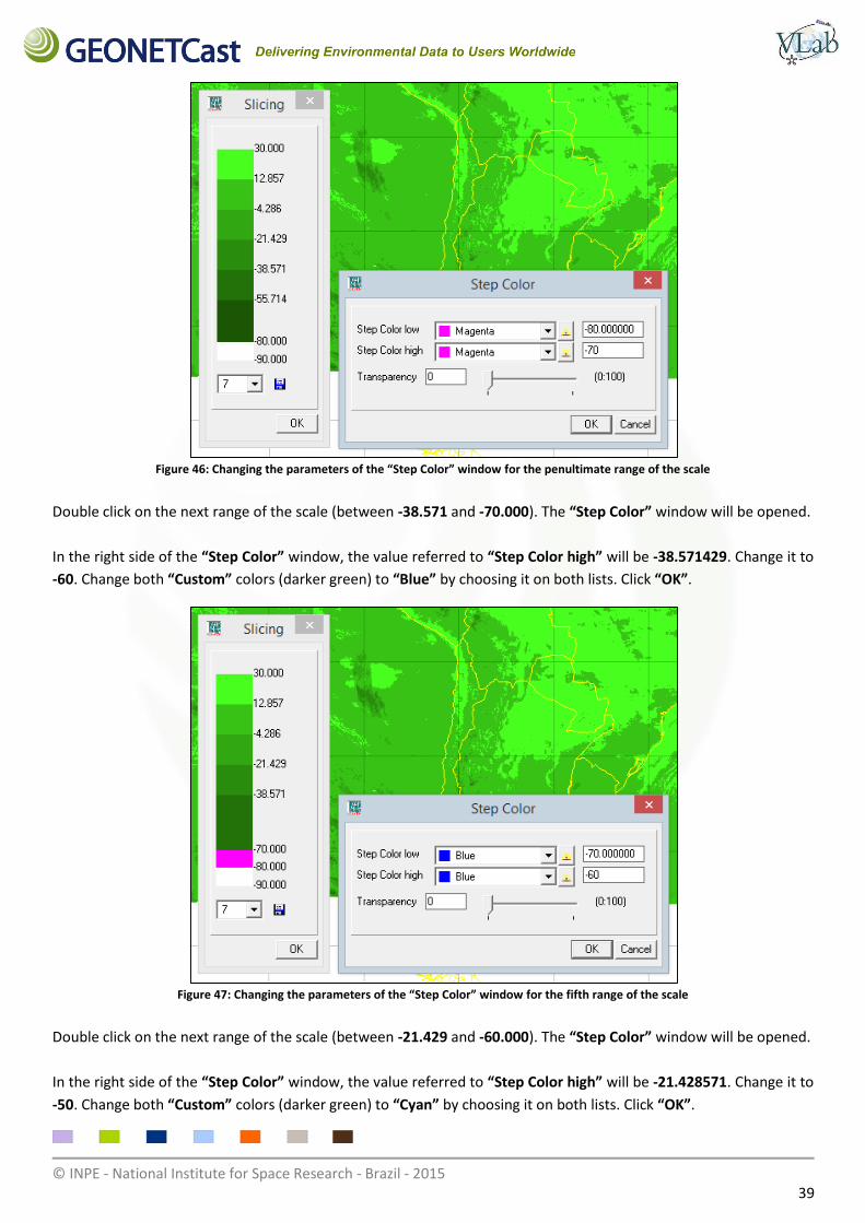
Figure 46: Changing the parameters of the “Step Color” window for the penultimate range of the scale
Double click on the next range of the scale (between -38.571 and -70.000). The “Step Color” window will be opened.
In the right side of the “Step Color” window, the value referred to “Step Color high” will be -38.571429. Change it to
-60. Change both “Custom” colors (darker green) to “Blue” by choosing it on both lists. Click “OK”.
Figure 47: Changing the parameters of the “Step Color” window for the fifth range of the scale
Double click on the next range of the scale (between -21.429 and -60.000). The “Step Color” window will be opened.
In the right side of the “Step Color” window, the value referred to “Step Color high” will be -21.428571. Change it to
-50. Change both “Custom” colors (darker green) to “Cyan” by choosing it on both lists. Click “OK”.
© INPE - National Institute for Space Research - Brazil - 2015 40
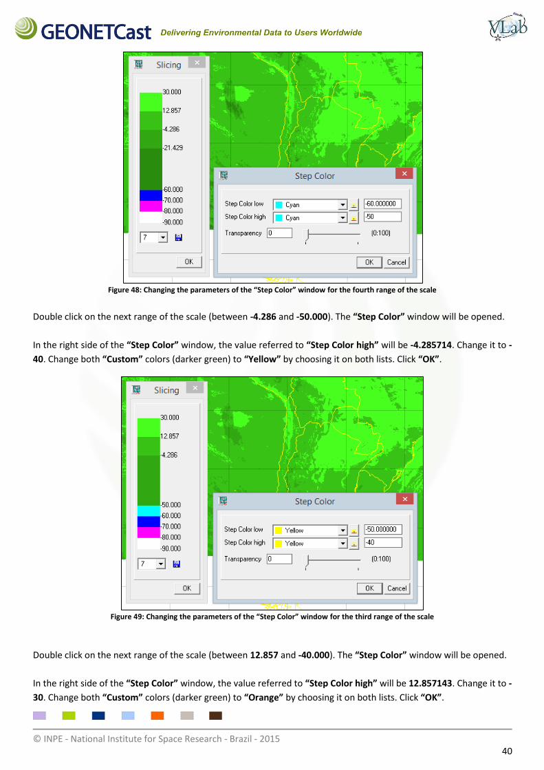
Figure 48: Changing the parameters of the “Step Color” window for the fourth range of the scale
Double click on the next range of the scale (between -4.286 and -50.000). The “Step Color” window will be opened.
In the right side of the “Step Color” window, the value referred to “Step Color high” will be -4.285714. Change it to -
40. Change both “Custom” colors (darker green) to “Yellow” by choosing it on both lists. Click “OK”.
Figure 49: Changing the parameters of the “Step Color” window for the third range of the scale
Double click on the next range of the scale (between 12.857 and -40.000). The “Step Color” window will be opened.
In the right side of the “Step Color” window, the value referred to “Step Color high” will be 12.857143. Change it to -
30. Change both “Custom” colors (darker green) to “Orange” by choosing it on both lists. Click “OK”.
© INPE - National Institute for Space Research - Brazil - 2015 41
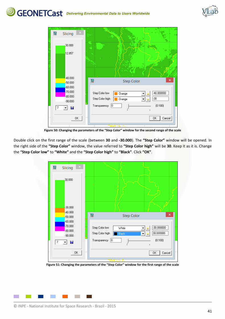
Figure 50: Changing the parameters of the “Step Color” window for the second range of the scale
Double click on the first range of the scale (between 30 and -30.000). The “Step Color” window will be opened. In
the right side of the “Step Color” window, the value referred to “Step Color high” will be 30. Keep it as it is. Change
the “Step Color low” to “White” and the “Step Color high” to “Black”. Click “OK”.
Figure 51: Changing the parameters of the “Step Color” window for the first range of the scale

© INPE - National Institute for Space Research - Brazil - 2015 42
The resulting image will be displayed as follows:
Figure 52: The resulting image, enhanced to facilitate the interpretation
To save the newly created color palette, click on the floppy symbol in the “Slicing” window. In ILWIS, a color palette
is called “representation”. Save your new representation (.rpr file) in your preferred folder (e.g.: “C:\VLAB”). In this
example we will save it as “Infrared_Enhance.rpr”.
Figure 53: Floppy symbol used to save your representation
© INPE - National Institute for Space Research - Brazil - 2015 43
Hint: You may find the standard ILWIS representations in: “C:\Program Files (x86)\n52\ILWIS38\system”. You
may save the representations created by you in this folder.
Now you may use this same color palette (“Infrared_Enhance.rpr”) to enhance infrared images in Celsius from any
satellite, including those from the GEONETCast-Americas broadcast!
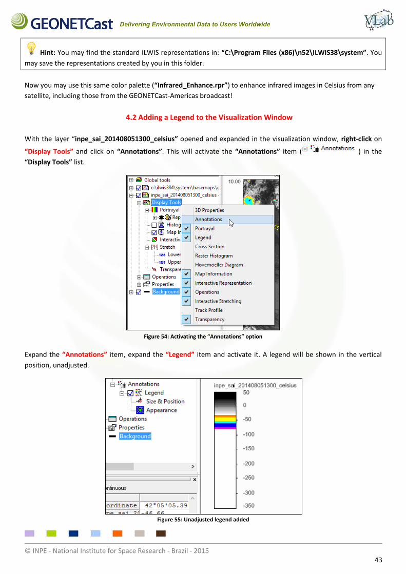
4.2 Adding a Legend to the Visualization Window
With the layer “inpe_sai_201408051300_celsius” opened and expanded in the visualization window, right-click on
“Display Tools” and click on “Annotations”. This will activate the “Annotations” item ( ) in the
“Display Tools” list.
Figure 54: Activating the “Annotations” option
Expand the “Annotations” item, expand the “Legend” item and activate it. A legend will be shown in the vertical
position, unadjusted.
Figure 55: Unadjusted legend added
© INPE - National Institute for Space Research - Brazil - 2015 44
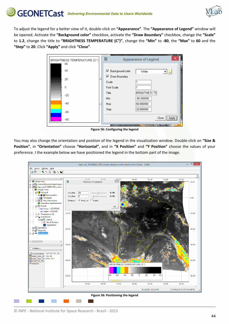
To adjust the legend for a better view of it, double-click on “Appearance”. The “Appearance of Legend” window will
be opened. Activate the “Background color” checkbox, activate the “Draw Boundary” checkbox, change the “Scale”
to 1.2, change the title to “BRIGHTNESS TEMPERATURE (C°)”, change the “Min” to -80, the “Max” to 60 and the
“Step” to 20. Click “Apply” and click “Close”.
Figure 56: Configuring the legend
You may also change the orientation and position of the legend in the visualization window. Double-click on “Size &
Position”, in “Orientation” choose “Horizontal”, and in “X Position” and “Y Position” choose the values of your
preference. I the example below we have positioned the legend in the bottom part of the image.
Figure 56: Positioning the legend
© INPE - National Institute for Space Research - Brazil - 2015 45
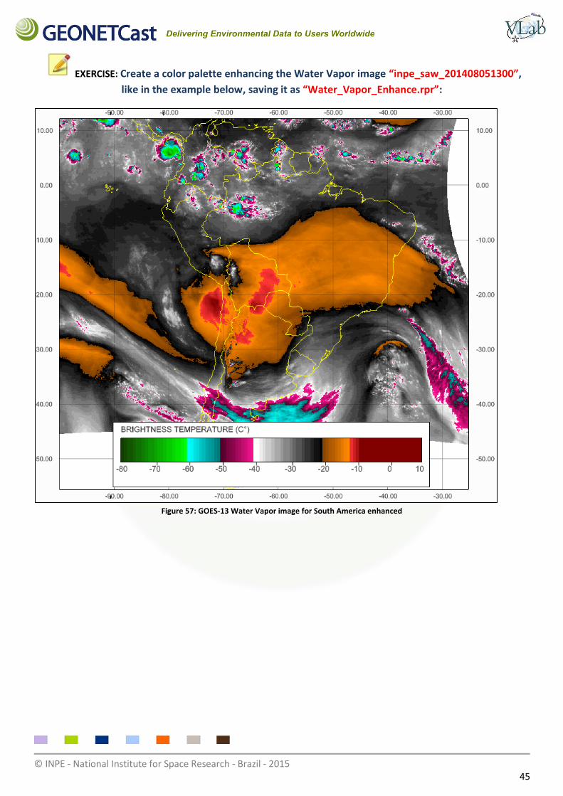
EXERCISE: Create a color palette enhancing the Water Vapor image “inpe_saw_201408051300”,
like in the example below, saving it as “Water_Vapor_Enhance.rpr”:
Figure 57: GOES-13 Water Vapor image for South America enhanced