Geometry of Quantum States fromSymmetric Informationally Complete

Probabilities

by

Gelo Noel M. Tabia

A thesispresented to the University of Waterloo

in fulfillment of thethesis requirement for the degree of

Doctor of Philosophyin

Physics - Quantum Information

Waterloo, Ontario, Canada, 2013

c© Gelo Noel M. Tabia 2013

I hereby declare that I am the sole author of this thesis. This is a true copy of the thesis,including any required final revisions, as accepted by my examiners.

I understand that my thesis may be made electronically available to the public.

ii

Abstract

It is usually taken for granted that the natural mathematical framework for quantummechanics is the theory of Hilbert spaces, where pure states of a quantum system corre-spond to complex vectors of unit length. These vectors can be combined to create moregeneral states expressed in terms of positive semidefinite matrices of unit trace called den-sity operators. A density operator tells us everything we know about a quantum system.In particular, it specifies a unique probability for any measurement outcome. Thus, tofully appreciate quantum mechanics as a statistical model for physical phenomena, it isnecessary to understand the basic properties of its set of states. Studying the convex ge-ometry of quantum states provides important clues as to why the theory is expressed mostnaturally in terms of complex amplitudes. At the very least, it gives us a new perspectiveinto thinking about structure of quantum mechanics.

This thesis is concerned with the structure of quantum state space obtained from thegeometry of the convex set of probability distributions for a special class of measurementscalled symmetric informationally complete (SIC) measurements. In this context, quantummechanics is seen as a particular restriction of a regular simplex, where the state space ispostulated to carry a symmetric set of states called SICs, which are associated with equian-gular lines in a complex vector space. The analysis applies specifically to 3-dimensionalquantum systems or qutrits, which is the simplest nontrivial case to consider according toGleason’s theorem. It includes a full characterization of qutrit SICs and includes specificproposals for implementing them using linear optics. The infinitely many qutrit SICs areclassified into inequivalent families according to the Clifford group, where equivalence isdefined by geometrically invariant numbers called triple products. The multiplication ofSIC projectors is also used to define structure coefficients, which are convenient for elu-cidating some additional structure possessed by SICs, such as the Lie algebra associatedwith the operator basis defined by SICs, and a linear dependency structure inherited fromthe Weyl-Heisenberg symmetry. After describing the general one-to-one correspondencebetween density operators and SIC probabilities, many interesting features of the set ofqutrits are described, including an elegant formula for its pure states, which reveals a per-mutation symmetry related to the structure of a finite affine plane, the exact rotationalequivalence of different SIC probability spaces, the shape of qutrit state space defined bythe radial distance of the boundary from the maximally mixed state, and a comparison ofthe 2-dimensional cross-sections of SIC probabilities to known results. Towards the end,the representation of quantum states in terms of SICs is used to develop a method forreconstructing quantum theory from the postulate of maximal consistency, and a proce-dure for building up qutrit state space from a finite set of points corresponding to a Hesseconfiguration in Hilbert space is sketched briefly.

iii

Acknowledgements

There is no one way the world is because the world is still in creation, stillbeing hammered out.

– Christopher A. Fuchs, letter to Howard Barnum and Tony Sudbury, August18, 2003, quoted in Scientific American, Sept. 2004

I wish to express my sincerest gratitude to my advisor Chris Fuchs, for having providedme the opportunity and the privilege of working with him in my pursuit of a doctoraldegree. I will always feel greatly indebted to him, since he was willing to take a chance onme four years ago when I had been looking for a supervisor for almost a year to no avail.Chris is an excellent advisor, who cares not just about how much work his students getdone but also in their general well-being. I have personally benefitted from his valuableinsights and sage advice on what problems to look at or what next steps to consider.His knowledge, guidance, patience and support have been invaluable to my research andstudies. But I think just as important is his overall influence in my way of thinking andapproach to physics and life. I feel some of the important lessons I have learned from him,which are worth mentioning here:

(i) Do not be afraid to ask silly questions. True, they are usually a waste of other people’stime but occasionally they turn out not to be silly at all.

(ii) Be constructive, not just productive. Do not fall into the trap of busywork.

(iii) When you obtain a result that is simpler than you expected, find out why.

(iv) Do not be satisfied with vague claims based on intuition. Always demand precisionand some rigorous mathematics.

(v) But while mathematics is important, remember that often the most profound ideasin physics can be expressed meaningfully with a few, well-chosen words.

It is my sincere hope that these lessons, taken to heart, bring me a few steps closer to thekind of physicist he is.

I would like to extend my special thanks to Marcus Appleby, Asa Ericsson, Hoan Dang,and Matthew Graydon, friends and comrade-in-arms in research topics related to SICs. ToMarcus and Asa, I am grateful for their willingness to discuss many of my ideas, mostof which did not work, and for sharing their valuable insight into various problems that

iv

I have struggled with in my research. To Hoan and Matthew, I am grateful for all thetime we spent as students of Chris, for all the enlightening and enjoyable conversations onboth physics and non-physics matters alike, and for the tradition of attending APS MarchMeetings, which I hope continues for many more years.

I would like to thank Norbert Lutkenhaus, Kevin Resch, Joseph Emerson, and AndrewChilds for serving in my PhD committee and for always making sure I was always on trackin fulfilling the requirements of my program. I would also like to thank Ingemar Bengtssonfor acting as the external examiner for my thesis defense. His work on the geometry ofquantum states has been a source of inspiration to my research and it is an honor and aprivilege to have him evaluate my contributions to the field.

Each of the following have in one way or another, influenced this thesis, sometimesdirectly in its content but even if only in little ways that affected its emphasis on certainideas: Berge Englert, Zach Medendorp, Christoph Schaeff, Bill Wootters, Rob Spekkens,Lucien Hardy, Jeff Bub, John Watrous, Ben Reichardt, Frank Wilhelm, and HuangjunZhu.

I am grateful to the Perimeter Institute for providing a stimulating environment forresearch, and its staff in particular, for the numerous times they have assisted me onadministrative matters. I would like to mention in particular my officemates Jeff Hnybidaand Katja Reid, for many delightful and stimulating conversations about their own workand other things, which provide a short reprieve from the mostly tedious part of researchthat happens on my desk.

Special thanks to Alfonso Cesar Albason, a companion from distance in my journeythrough my graduate studies. Getting a PhD is hard when you have many concerns anddistractions beyond research and having a friend to talk to who understands the experienceis both helpful and encouraging.

My continuing education would not be possible without the unwavering support andunderstanding of my dearest family and closest friends, for the many times they haveencouraged me to carry on when things became difficult, and for relieving some of thepressures of those hard and trying moments. Many thanks to them.

v

To the loving memory of my father, Angel Garrucha Tabia, Jr.

vi

Table of Contents

List of Tables xi

List of Figures xii

1 Introduction 1

1.1 Historical background and motivation . . . . . . . . . . . . . . . . . . . . . 2

1.2 Research scope and objectives . . . . . . . . . . . . . . . . . . . . . . . . . 7

1.3 Roadmap for the thesis . . . . . . . . . . . . . . . . . . . . . . . . . . . . . 9

1.4 List of specific contributions . . . . . . . . . . . . . . . . . . . . . . . . . . 10

2 Overview of quantum mechanics 11

2.1 Outline of the quantum formalism . . . . . . . . . . . . . . . . . . . . . . . 12

2.2 Qubits and the Bloch ball . . . . . . . . . . . . . . . . . . . . . . . . . . . 16

2.3 The set of density operators . . . . . . . . . . . . . . . . . . . . . . . . . . 17

3 SIC-POVMs and Weyl-Heisenberg qutrit SICs 22

3.1 Characterizing SIC-POVMs . . . . . . . . . . . . . . . . . . . . . . . . . . 23

3.1.1 Equiangular lines . . . . . . . . . . . . . . . . . . . . . . . . . . . . 23

3.1.2 Complex projective design . . . . . . . . . . . . . . . . . . . . . . . 25

3.1.3 Maximal equiangular tight frame . . . . . . . . . . . . . . . . . . . 26

3.2 Weyl-Heisenberg SICs and the Clifford group . . . . . . . . . . . . . . . . . 28

vii

3.3 Classifying qutrit SICs into inequivalent families . . . . . . . . . . . . . . . 30

3.4 Geometric invariants of qutrit SICs . . . . . . . . . . . . . . . . . . . . . . 32

3.5 Linear dependency structure of qutrit SICs . . . . . . . . . . . . . . . . . . 40

3.6 The Zauner subspace for qutrit SICs . . . . . . . . . . . . . . . . . . . . . 45

3.7 Lie algebraic properties of qutrit SICs . . . . . . . . . . . . . . . . . . . . . 47

4 Practical implementations of SIC-POVMs 53

4.1 Experimental SICs using optimal polarimetry . . . . . . . . . . . . . . . . 54

4.2 Implementing SICs by successive measurements . . . . . . . . . . . . . . . 56

4.3 Storage loop SIC- POVM experiment with weak projections . . . . . . . . 59

4.4 Multiport scheme from Naimark dilation of SIC-POVMs . . . . . . . . . . 62

4.4.1 Multiport Qubit SIC-POVM . . . . . . . . . . . . . . . . . . . . . . 63

4.4.2 Multiport Qutrit SIC-POVM . . . . . . . . . . . . . . . . . . . . . 65

4.4.3 Remarks on improvements and feasibility . . . . . . . . . . . . . . . 70

5 The SIC representation of quantum states 73

5.1 Quantum states as degrees of belief . . . . . . . . . . . . . . . . . . . . . . 74

5.2 Representing quantum states with SICs . . . . . . . . . . . . . . . . . . . . 76

5.3 Pure states as fixed points of a map . . . . . . . . . . . . . . . . . . . . . . 79

5.4 Pure states as stationary points of a map . . . . . . . . . . . . . . . . . . . 81

5.5 Rotations relating different SIC representations . . . . . . . . . . . . . . . 86

5.6 Fidelity of quantum states . . . . . . . . . . . . . . . . . . . . . . . . . . . 88

5.7 Purification of mixed states . . . . . . . . . . . . . . . . . . . . . . . . . . 92

5.8 Entanglement in 2-qubit systems . . . . . . . . . . . . . . . . . . . . . . . 97

5.9 Quantum operations as affine maps on SIC probabilities . . . . . . . . . . 103

viii

6 Geometric features of qutrit state space 112

6.1 Qutrit pure states in terms of SICs . . . . . . . . . . . . . . . . . . . . . . 113

6.2 Rotations between qutrit state spaces . . . . . . . . . . . . . . . . . . . . . 114

6.3 A permutation symmetry for qutrit pure states . . . . . . . . . . . . . . . 116

6.4 The boundary of qutrit state space . . . . . . . . . . . . . . . . . . . . . . 119

6.5 Plane sections of qutrit state space . . . . . . . . . . . . . . . . . . . . . . 124

7 Quantum state space as a maximal consistent set 131

7.1 Quantum states from the Born rule . . . . . . . . . . . . . . . . . . . . . . 132

7.2 General maximal consistent sets . . . . . . . . . . . . . . . . . . . . . . . . 135

7.3 Properties of maximal consistent sets . . . . . . . . . . . . . . . . . . . . . 144

7.4 Maximization of consistent sets: examples . . . . . . . . . . . . . . . . . . 149

7.5 Qutrit state space as a maximal consistent set . . . . . . . . . . . . . . . . 156

7.6 Duality and symmetry of maximal consistent sets . . . . . . . . . . . . . . 165

8 Summary and outlook 169

8.1 Recap of main results . . . . . . . . . . . . . . . . . . . . . . . . . . . . . . 170

8.1.1 Practical implementation of SICs . . . . . . . . . . . . . . . . . . . 170

8.1.2 Characterizing states in the SIC representation . . . . . . . . . . . 170

8.1.3 A most exceptional SIC for qutrits . . . . . . . . . . . . . . . . . . 172

8.1.4 Maximal consistent sets and quantum states . . . . . . . . . . . . . 173

8.2 List of unresolved questions . . . . . . . . . . . . . . . . . . . . . . . . . . 174

8.3 Closing remarks . . . . . . . . . . . . . . . . . . . . . . . . . . . . . . . . . 176

APPENDICES 178

A From sets to probabilities 179

B Convex sets in real Euclidean spaces 189

ix

C Basic facts about linear operators 191

D Measuring distances between probability distributions 193

E Theory of filters and transition probabilities 197

F Projective geometry of quantum phase space 202

References 206

x

List of Tables

3.1 Distinct values for Sijk given parameter t. . . . . . . . . . . . . . . . . . . 35

3.2 Structure coefficient index generators for qutrit SICs. The index triples (ijk) for

each value of Sijk are obtained from rules that make use of these index generators. 37

3.3 Linear dependency structures for the most exceptional SIC in d = 3. Thevectors |j〉 correspond to SIC vectors and are labeled according to Eq. (3.43). 42

3.4 Good p-sets yielding linear dependencies for the 8 SICs with t = π9 . . . . . . . . 44

6.1 Plane cross-sections of the SIC probability space matched to Kimura’s classifica-

tion. All remaining cross-sections are Type IV(r2i + r2

j = 49

). . . . . . . . . . . 127

6.2 The 28 plane sections arranged according to type, with ij specifying thesubspace spanned by (λi, λj). . . . . . . . . . . . . . . . . . . . . . . . . . 128

A.1 Boolean laws on sets . . . . . . . . . . . . . . . . . . . . . . . . . . . . . . 181

xi

List of Figures

3.1 Qubit SIC-POVM on the Bloch sphere is represented by the vertices of aninscribed tetrahedron. Reproduced from [8]. . . . . . . . . . . . . . . . . . 23

4.1 Implementing a continuous family of SICs for a path-encoded qutrit usingsuccessive measurements. Image reproduced from Ref. [71] . . . . . . . . . 58

4.2 SIC-POVM storage loop scheme implemented by partial projections overthree round trips. The PPBS labels indicate how the detector click is inter-preted. . . . . . . . . . . . . . . . . . . . . . . . . . . . . . . . . . . . . . 60

4.3 (a) Qutrit state encoding. (b) Implementing the X and Z gates. . . . . . 60

4.4 Schematic for the storage loop SIC experiment. . . . . . . . . . . . . . . . 61

4.5 Schematic for a multiport qubit SIC-POVM experiment. . . . . . . . . . . 64

4.6 Qubit SIC-POVM implemented with an optical multiport device. . . . . . 66

4.7 Schematic for a qutrit SIC-POVM generated by Eq.(4.43) using multiportdevices. . . . . . . . . . . . . . . . . . . . . . . . . . . . . . . . . . . . . . 69

4.8 Multiport circuit for the unitary operators Q†k. The circuits for Q†k differ only

by a phase shift and a relabeling of output modes according to Gk. The output

modes shown are for Q†1. . . . . . . . . . . . . . . . . . . . . . . . . . . . . . 70

5.1 Purifying qubit mixed states in the SIC representation. In solving for thepurification of σ, it is best to use a qubit SIC with an element ‘parallel’ to σ. 96

6.1 The index triples (ijk) for the pure states of the most exceptional SIC,depicted as the 12 lines of a finite affine plane over GF(3), where each pointrepresents an index. . . . . . . . . . . . . . . . . . . . . . . . . . . . . . . . 114

6.2 A plot of F as a function of one of the eigenvalues α for boundary states. . . . . 122

xii

6.3 The radial distance r of boundary states from the maximally mixed state, as a

function of F = F (~n). . . . . . . . . . . . . . . . . . . . . . . . . . . . . . . 123

6.4 2-dimensional cross-sections of the SIC probability space corresponding to Types

I, II, III, and IV, in Kimura’s classification. The yellow shaded regions represent

valid quantum states. The axes correspond to 2 parameters that define the 2-

dimensional subspace for the SIC probabilities given in Table 6.1. . . . . . . . 130

7.1 A conceptual diagram for the Born rule in terms of a SIC. It shows how theBorn rule relates a counterfactual SIC measurement in the sky with somearbitrary measurement on the ground. . . . . . . . . . . . . . . . . . . . . 132

7.2 Gumdrop with an insphere of radius c√k

and an outsphere of√k. The light

gray area is a cross section of Conv(S ∪ T ). . . . . . . . . . . . . . . . . . . 144

7.3 Regular triangle on a plane as a maximal consistent set. . . . . . . . . . . 154

E.1 Transition probability from filters . . . . . . . . . . . . . . . . . . . . . . . 198

E.2 Representing transition probabilities with S(2, n). . . . . . . . . . . . . . . 199

E.3 Isomorphism between S(2, 2) and H2(R) via stereographic projection. . . . . . . 200

E.4 Isomorphism between S(2, 3) and H2(C) via stereographic projection. . . . . . . 201

xiii

Chapter 1

Introduction

Why does quantum mechanics have the structure that it has? In particular, why arequantum systems most convenient to describe in terms of linear operators and complex-valued probability amplitudes? John Wheeler tells us that it follows from two distinctivefeatures of quantum phenomena: a complementary choice of questions to ask each quantumsystem, and answers to those questions that must be deduced from probabilities [129].

As Wheeler points out, Ronald Fisher has taught us that the correct number to deter-mine from experiments is not the probability of the desired answer but its square root [38].The need to adequately distinguish between nearly identical sets of measurement statisticsis what then leads to the notion of statistical distance. In Hilbert space, this translatesinto the angle θ between two probability amplitude vectors |ψ〉 and |φ〉 given by

θ = arccos |〈ψ|φ〉|. (1.1)

Ernst Stuckelberg showed that probability amplitudes that are exclusively real are incom-patible with Heisenberg’s uncertainty relations [123]. Equivalently, Wheeler has arguedthat this means that they are incompatible with Bohr’s complementarity principle.

Yet since the only truly observable quantities in the theory are the outcome proba-bilities of measurements and not the amplitudes, it must be possible to understand theHilbert space structure solely in terms of probabilities. William Wootters gives such adescription in terms of the probability tables of mutually unbiased bases, where the role ofcomplex amplitudes in transition probabilities are replaced by “coincidence sums” betweenprobability tables [133]. In this thesis, we formulate quantum theory using probability dis-tributions obtained from symmetric, informationally complete (SIC) measurements andhighlight the geometric properties of quantum states exhibited in this framework.

1

1.1 Historical background and motivation

In a 1926 paper, Max Born proposed the statistical interpretation of quantum mechanicsthat is with us to this day [20]. In his discussion of a scattering problem, he mentions ina footnote that the probability of a specific outcome is obtained from the square of theSchrodinger wave function. In modern parlance, we would write

p(x) = |〈x|ψ〉|2 (1.2)

for the probability of getting outcome x given that the system being measured is describedby the state |ψ〉. Put differently, p(x) gives the transition probability of finding the systemin state |x〉 when it was in state |ψ〉 before measurement. Once probabilities enter intothe picture, we know that we are dealing with a statistical theory, where the outcomes ofcertain measurements are nondeterministic.

Even in the formative years of quantum mechanics, physicists wondered about thephysical meaning behind this underlying indeterminism. For his part, Werner Heisenbergargued that quantum randomness is a consequence of having to ascribe a conjugate pairof variables to each physical degree of freedom, where the simultaneous values of the twovariables can only be determined with some irreducible uncertainty [62]. In his matrixmechanics, this follows from the canonical commutation relation

[X,P ] = i~, (1.3)

where X and P refer to any such conjugate pair. Here we clearly see that complex numbersplay a necessary and prominent role in quantum theory.

Around the same time as this particular assertion by Heisenberg, Niels Bohr formulatedthe principle of complementarity [18], a concept concerning wave and particle aspects ofquantum systems. To Bohr, the uncertainty relations were manifestations of the deeperprinciple of complementarity, a claim duly noted by Heisenberg in an addendum to hispaper on the uncertainty principle. Complementarity can be made formally precise inwhich-way experiments in quantum optics [120], where the complementary observables forpath distinguishability D and interference pattern visibility V have been shown to obeythe duality relation [35]

D2 + V 2 ≤ 1. (1.4)

However, despite its profound significance, the complementarity principle does not reallyhelp us understand why the probabilities are obtained from complex amplitudes. To dothat, we need a more general and systematic way to explore the function of complexnumbers in the theory, which we gain when we use Hilbert spaces.

2

Hilbert spaces were first introduced into quantum mechanics by David Hilbert, LotharNordheim, and John von Neumann [63] in 1927 in a collaborative effort to make thetransformation theory of Pascual Jordan and Paul Dirac more mathematically rigorous.The familiar form we learn today was first established by von Neumann in a follow-uppaper [127].

In finite dimensions, Hilbert space is just a complex vector space supplied with aninner product. Hilbert space represents a significant and useful advance in quantum theorybecause much of the geometric intuition learned from Euclidean geometry still applies to it.For example, an exact analog of the Pythagorean theorem holds for Hilbert spaces. Also,vectors in a Hilbert space can be uniquely specified with respect to a coordinate system inexactly the same way Cartesian coordinates can be assigned to points on a plane. Linearoperators on Hilbert spaces are likewise easy to visualize as certain transformations thatstretch or shrink the space in different directions.

To connect the abstract notions of Hilbert space to concrete facts about measurementsand observations in quantum theory, Garrett Birkhoff and John von Neumann developedthe idea of a logic of questions about properties of a quantum system that can be checkedwith yes-no measurements [17]. They demonstrated that quantum properties exhibit thealgebraic structure of an orthocomplemented lattice, which translates into a representationof states in terms of projection operators on a Hilbert space.

While the discovery of quantum logic is a nice and important result, it would be hardlyenlightening or satisfying for anyone to claim that the laws of quantum mechanics originatefrom the distinct, non-Boolean flavor of its logical propositions. What we really desire is amore intuitive way to understand the role of the complex amplitudes in the indeterminismimplied by quantum laws. In particular, what sort of statistical theory is implied by theHilbert space structure of quantum mechanics?

Bogdan Mielnik taught us that the true lesson from quantum logic is that there is a moregeneral way to describe the statistical properties of quantum ensembles using geometricalconcepts. In particular, he showed that if we interpret logical propositions in terms offilters that transmit beams of particles of a specific type, the Born rule becomes a purelygeometric constraint on the absorption coefficient, or transition probability, between pairsof filters [99]. The resulting space of transition probabilities is equivalent to Hilbert space ifthe structure of its 2-dimensional subspaces lead to the usual linear superposition principle.1

This allows us to consider state spaces whose geometries do not admit a Hilbert spacerepresentation, something that might be relevant in attempts to develop a working theoryof quantum gravity.

1 Details on this can be found in Appendix E.

3

In general, we can assign to any statistical theory a geometric description where statesare represented by points of a convex set S, which we consider to be a subset of the realEuclidean space Rn. If we take a pair of states ~x1, ~x2 ∈ S then the state x = p1~x1 + p2~x2

denotes a mixture of the states ~x1 and ~x2 in proportions given by the probabilities p1 andp2, respectively. Because the set is convex, any point lying on the line segment joining anypair of points in S also belongs in S. On the boundary of S, there are special points thatcan not be expressed as a nontrivial combination of other states and are called extremepoints. Because these points do not represent mixtures of different states, we call them purestates. We assume that the set S is compact, which means that every state correspondingto some point in S can be written as a finite convex combination of pure states.

In classical mechanics, the convex set describing the state space of a system with Nperfectly distinguishable states is given by the set of probability vectors on a regular sim-plex ∆N−1. The vertices of the simplex are associated with classical pure states, and anymixture has a unique decomposition in terms of these pure states. In a typical settingof classical dynamics where states refer to continuous degrees of freedom, such as posi-tion and momentum, the simplices are not only infinite-dimensional, they also possess akind of symplectic structure that accommodates canonical transformations by Hamiltonianfunctions.

In quantum mechanics, the simplest convex set is a 3-dimensional ball called the Blochball; it is the state space for 2-dimensional quantum systems, or qubits. The points on thesurface of the Bloch ball represent pure states while the interior corresponds to mixtures.Relations among qubit density operators on a Hilbert space translate into specific geometricproperties of the Bloch ball. For instance, orthogonal states correspond to antipodal pointson the sphere. Also, any mixture can be obtained from mixing any pair of pure stateslying on the line segment passing through the point representing that mixture. Thus,even in the simplest case, the geometry of the convex set of quantum states expresses theindistinguishability of quantum mixtures, a phenomenon shared by any statistical theorywith a state space that is not equivalent to a probability simplex. That is, given anymixture, it is impossible to physically distinguish between two different ways of combiningstates that lead to the same mixed state.

Although the geometry of the Bloch ball is elegant, it is actually too simple. In fact,there is a specific sense in which it is not representative of the convex geometry we expectfrom quantum theory. This is embodied in two important foundational results concerningthe structure of probabilities in quantum mechanics: Gleason’s theorem [51] and the Bell-Kochen-Specker theorem [9, 82]. Gleason’s theorem states that the Born rule specifyingthe probabilities for the outcomes of quantum measurements is the only possible wayto obtain them from density operators. In particular, Andrew Gleason proved that the

4

theorem holds in all finite dimensions if and only if it holds in d = 3. On the other hand,the Bell-Kochen-Specker theorem states that assigning simultaneous non-contextual valuesto all quantum observables is impossible. It can be proven as a corollary to Gleason’stheorem [22]. Together the theorems suggest that an accurate picture of the complexstructure of quantum states can only be gleaned from Hilbert spaces that are at least3-dimensional. Thus, in formulating a geometric framework for understanding quantumprobabilities, we will employ qutrits as our case study for explicit calculations and analysis.

Several authors have examined cross-sections of qutrit state space in order to gainsome insights into the rich, intricate geometry of quantum states, most notably the workby Sandeep Goyal, et. al, which gives a comprehensive analysis of the 2- and 3-dimensionalcross-sections of the generalized Bloch ball [56]. An important part of their results clarifiesthe connection between a cross-section forming an obese tetrahedron and the tetrahedralsymmetry represented by a group of signed permutation matrices. Gniewomir Saribickiand Ingemar Bengtsson supplement Goyal, et al. by classifying all possible 2-dimensionalcross-sections of a qutrit in terms of the plane cubic curve that defines the boundary ofevery such cross-section [115].

Despite the great strides made in recent years in our understanding of the convex ge-ometry of qutrits, much of what we have determined involves specific observations thatdo not necessarily clarify why, for instance, the space of quantum states have a positivitystructure and unitary symmetry, and what are the implications of these features for thecorresponding statistical theory. Particularly, we are still searching for a simple and intu-itive geometric characterization of shape of qutrit state space that generalizes to all finitedimensions, similar to how we know that all classical state spaces are regular simplices.

It may be worth mentioning here that despite the somewhat limited scope of examiningjust qutrits, a better understanding of qutrits is important even beyond their relevancein foundational studies of quantum mechanics. In fact, qutrits play essential roles invarious applications of quantum information theory. This may come as a bit of a surprisesince the vast majority of quantum information processing is designed for and achieved bymanipulating qubits but there are several instances when qutrits are necessary in principle.Some examples are

(a) the optimal solution to the Byzantine agreement problem requires entangled qutrits[39,48],

(b) a quantum computer with a finite number of distinguishable states has a maximalHilbert space if it is partitioned into qutrits [58],

5

(c) threshold schemes for quantum secret sharing work only if the quantum system usedfor the secret is at least 3-dimensional [28],

(d) quantum key distribution with qutrits provides increased coding density and a highersecurity margin for errors [59],

(e) recently it has been shown that the smallest possible heat engines involves a qutritwith spatially separated basis states [86], and

(f) qutrits are more robust under certain forms of decoherence, making them suitable forstoring quantum information [96].

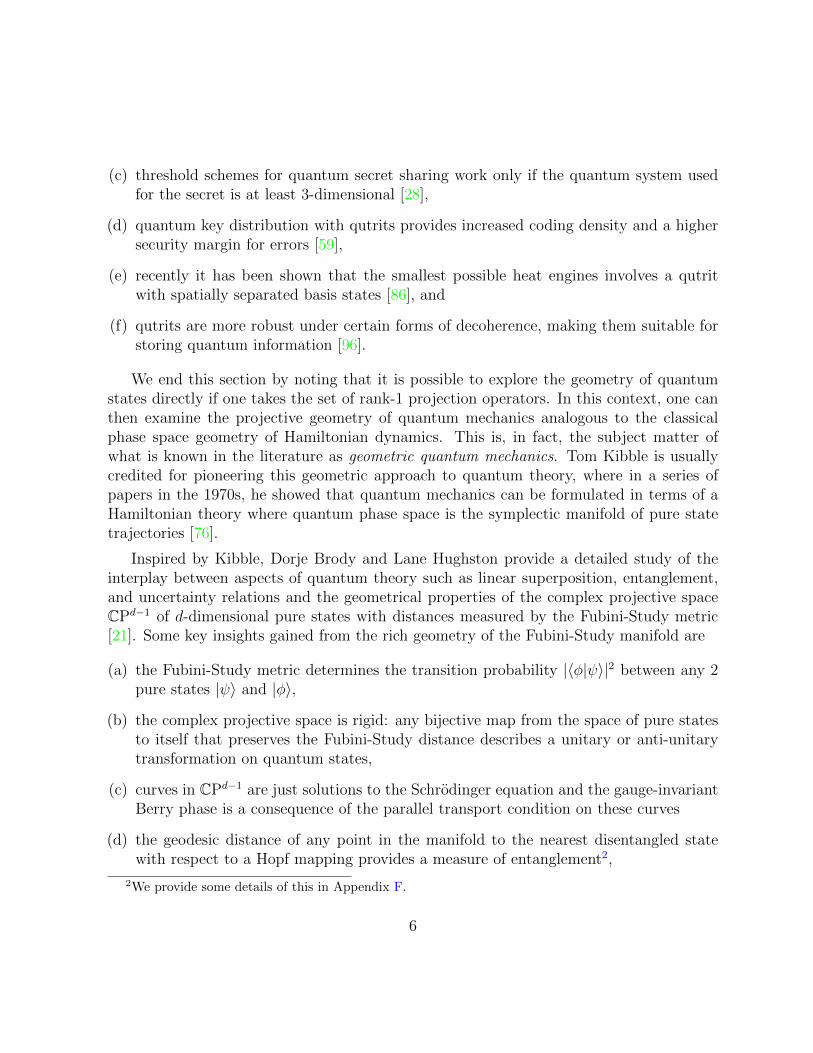
We end this section by noting that it is possible to explore the geometry of quantumstates directly if one takes the set of rank-1 projection operators. In this context, one canthen examine the projective geometry of quantum mechanics analogous to the classicalphase space geometry of Hamiltonian dynamics. This is, in fact, the subject matter ofwhat is known in the literature as geometric quantum mechanics. Tom Kibble is usuallycredited for pioneering this geometric approach to quantum theory, where in a series ofpapers in the 1970s, he showed that quantum mechanics can be formulated in terms of aHamiltonian theory where quantum phase space is the symplectic manifold of pure statetrajectories [76].

Inspired by Kibble, Dorje Brody and Lane Hughston provide a detailed study of theinterplay between aspects of quantum theory such as linear superposition, entanglement,and uncertainty relations and the geometrical properties of the complex projective spaceCPd−1 of d-dimensional pure states with distances measured by the Fubini-Study metric[21]. Some key insights gained from the rich geometry of the Fubini-Study manifold are

(a) the Fubini-Study metric determines the transition probability |〈φ|ψ〉|2 between any 2pure states |ψ〉 and |φ〉,

(b) the complex projective space is rigid: any bijective map from the space of pure statesto itself that preserves the Fubini-Study distance describes a unitary or anti-unitarytransformation on quantum states,

(c) curves in CPd−1 are just solutions to the Schrodinger equation and the gauge-invariantBerry phase is a consequence of the parallel transport condition on these curves

(d) the geodesic distance of any point in the manifold to the nearest disentangled statewith respect to a Hopf mapping provides a measure of entanglement2,

2We provide some details of this in Appendix F.

6

(e) if we think of CPd−1 as a real manifold Γ with twice the dimension, then the structureof Γ is such that geometric inequalities for vector fields defined on Γ are equivalent toHeisenberg uncertainty relations for quantum observables, and

(f) geometric notions on the manifold of pure states can be extended to mixed states whenone considers purifications on a larger Hilbert space; for example, the Bures-Uhlmannmetric generalizes the notion of distances to all quantum states [126].

Although these are interesting observations, they do not help explain the why projectivegeometry applies to quantum mechanics, since here it is assumed at the onset. What thequantum phase space approach is most useful for is when we consider nonlinear modifica-tions to the Schrodinger equation. Most of the general features of the complex manifoldcarry over or can be adapted quite naturally to many aspects of the nonlinear regime.

1.2 Research scope and objectives

This thesis aims to establish some of the defining features of the of convex set of quantumstates by examining the structures and symmetries that come into view when quantumstates are expressed in terms of the probabilities for the outcomes of a symmetric, infor-mationally complete (SIC) measurement, a special class of measurement whose elementsare rank-1 projectors that form a set of d2 equiangular lines in Hilbert space. By repre-senting quantum states in terms of SICs, the full machinery of probability theory becomesimmediately applicable to the investigation of the properties of quantum state space.

Note that SICs also appear in various applications of quantum information, where theytypically play an important role in quantum state tomography and quantum cryptography.Thus, there is a strong interconnection among the foundational aspects surrounding thenature of quantum states, the mathematical aspects regarding the geometry of quantumstate space, and the practical aspects concerning the manipulation of quantum information,and SICs seem to play a vital, and potentially central, role in linking them together.

The nontrivial character of the geometry of quantum states is reflected most simply in3-dimensional quantum systems and so this research is devoted primarily to understandingthe structure of qutrits in all their intricate details, with some emphasis on the geometricalaspects. Particularly, the thesis attempts to address the following issues:

(i) Understand basic properties of SICs: Part of this research is concerned with unrav-eling the full symmetry of SICs by studying their connection with different areas

7

in mathematics such as projective geometry, finite field theory, and design theory.Such results may be of vital importance in efforts to construct a rigorous proof forthe existence of SICs in all dimensions. However, in this thesis, we focus our atten-tion on the geometric aspects of qutrit SICs with Weyl-Heisenberg symmetry, thedetails of which are most relevant in our subsequent analysis of the structure of thecorresponding state space.

(ii) Explore qutrits as a test bed for identifying general features of quantum state space:The structure of quantum probabilities follows from Gleason’s theorem, a result for di-mensions d ≥ 3 that assigns a unique probability measure to quantum states throughdensity operators. This suggests that the 3-dimensional case already contains theessential ingredients of the complex structure of quantum theory, making it appro-priate for initial studies. Some of our key results in this regard include an elegantformula for describing pure qutrits, a full listing of geometric invariants for qutritSICs and the rotational transformation between the probability vectors of distinctqutrit SICs, and a characterization of the shape of qutrit state space in terms of theradial distance of boundary states. Several results provide natural stepping stonesfor extended work in higher dimensions.

(iii) Develop experimental schemes for direct implementation of SIC measurements: Thevast majority of experiments in the lab involve projective measurements, which iswhy they are considered standard quantum measurements. However, advances inquantum information technology have shown that more ingenious measurements arepossible and it has only been recently that technology is up to the task in performingthem. Devising a practical implementation of SICs should provide a big boost formotivating them as canonical measurements. More generally, methods for realizingSICs in practice are potentially important for advancing experimental studies onhigher-dimensional quantum systems.

(iv) Reconstruct quantum theory from simple postulates: A better knowledge of the con-vex geometry of quantum states would highlight which basic features exhibit theprobabilistic structure of quantum theory, allowing us to deduce a set of physicallymotivated assumptions sufficient for recovering quantum mechanics from some mod-ification of classical probability theory. The specific approach we use takes the Bornrule as a normative postulate that formally leads to the idea of quantum state spaceas a maximal consistent set.

8

1.3 Roadmap for the thesis

The thesis provides a detailed analysis of the geometric structure of the convex body ofquantum states obtained from a representation of states in terms of SIC probabilities.

Chapter 2 presents an overview of quantum mechanics. It focuses on establishingthe quantum formalism in finite dimensions and discusses some general properties of thespace of density operators for qubits and higher dimensions, with emphasis on geometricfeatures such as its convex unitary structure and the Hilbert-Schmidt distance betweentwo operators. It includes a section on how quantum probabilities are obtained from analgebraic perspective.

Chapter 3 introduces symmetric informationally complete measurements in generaland Weyl-Heisenberg covariant qutrit SICs in particular. We define SICs as they appearin different contexts and characterize the group symmetry of SICs that are generated fromfiducial vectors. We classify qutrit SICs into eight families according to the independentorbits generated by the extended Clifford group and identify a SIC with the nicest prop-erties as the most exceptional SIC. We discuss various geometric aspects of SICs such asthe triple products that characterize unitary equivalence between SICs, the Lie algebraicproperties of the imaginary part of the triple products, and a linear dependency structureassociated with the Weyl-Heisenberg symmetry of qutrit SICs.

Chapter 4 describes various practical methods for implementing SICs. It includes theearlier polarimetry experiments of Thomas Durt, et al. on Wigner qubit tomography anda more recent experiment by Zach Medendorp, et al. using an optical storage loop withweak projections for simulating a qutrit SIC-POVM. We also discuss proposed methodsfor future experiments, one by Amir Kalev, et al. that describes a 2-step procedure witha fuzzy measurement followed by a projection onto the Fourier basis; the other one is myown proposed scheme using multiport devices designed to perform the Naimark extension,with specific designs for qubit and qutrit SICs.

Chapter 5 describes the SIC representation of quantum states, which we first motivate inthe framework of Quantum Bayesianism or QBism, where quantum states are characterizedas objects representing an agent’s degrees of belief about the future behavior of a quantumsystem. We then proceed to define pure quantum states in terms of SIC probabilities andobserve how this leads to a definition of pure states in terms of fixed and stationary pointsof certain linear maps. We also see how other physical quantities appear when expressedin the SIC language, such as the fidelity function used for distinguishing quantum statesand purification for mixed states. We also include a short discussion on entanglement inSIC terms, although limited to the partial positivity criterion for 2-qubit systems. We

9

end with a description of maps between density operators in terms of affine maps on thecorresponding SIC probability vectors.

Chapter 6 uses the SIC representation of qutrits to examine the geometric features ofqutrit state space. We see how the pure state conditions for the most exceptional SIC leadto an elegant formula for qutrit pure states. We construct the orthogonal transformationbetween the probability vectors of distinct SICs for the same quantum state in terms of a 3-dimensional circulant rotation matrix. We describe a permutation symmetry for qutrit SICprobabilities that provides some insight into the finite affine plane symmetry of qutrit purestates. We determine the boundary states of qutrits in terms of radial distance from theuniform distribution. We end with a discussion of the plane sections of SIC probabilities,which are shown to be equivalent to those obtained in the generalized Bloch representation.

Chapter 7 introduces the notion of a maximal consistent set in the context of postulatinga “quantum law of total probability” for extending classical probability theory to quantumtheory. We define a general notion of maximal consistent sets and show that classicaland quantum state spaces are important examples. We also describe general properties ofthese maximal consistent sets concerning convexity, boundary features, symmetry groupsand the notion of duality. We describe a method for reconstructing qutrit state space froma finite consistent set, where we show that a symmetry related to the Hesse configurationarises quite naturally.

Chapter 8 provides a summary of our key results, a list of problems recommended forfuture investigations, and some concluding remarks.

1.4 List of specific contributions

The results presented in this thesis representing my own specific contributions are containedin the following sections:

(i) Section 4.4 is based on GNM Tabia, Phys. Rev. A, 86 (2012) 062107.

(ii) Sections 3.3, 3.4, 5.5, 6.1, 6.2, and 6.4 are based on GNM Tabia and DM Appleby,Phys. Rev. A, 88 (2013) 012131.

(iii) Sections 3.5, 3.6, 3.7, 5.3, 5.4, 5.6, 5.7, 5.8, 5.9, 7.4, and 7.5 are based on unpublishedresearch notes.

10

Chapter 2

Overview of quantum mechanics

Quantum mechanics is considered to be one of humanity’s most impressive intellectualachievements. It certainly seems to be as mystifying as it is remarkable. To date, it is ourmost accurate scientific theory, capable of making predictions on the behavior of atomicscale objects with incredible precision. The mystery lies in what sort of picture quantumtheory paints about physical reality and a means of understanding in clear, unambiguousterms why Nature behaves the way it does.

Part of the reason why the interpretation remains unresolved is because the mathemat-ical structure of the theory, as established in the pioneering works of Erwin Schrodinger,Werner Heisenberg, Paul Dirac, and John von Neumann, does not naturally lead to a worldview that is fully consistent with intuitions developed in classical mechanics. This thesisis part of an attempt to better understand the implications of quantum theory as a formof probability calculus that applies to physical systems which can manifest nonclassicalphenomena such as interference and entanglement.

But in order to gain some appreciation for both the elegant and puzzling aspects ofquantum theory, it is necessary to get acquainted with the mathematics it employs, theframework of Hilbert spaces. Because we will not be concerned with systems with con-tinuous degrees of freedom, we focus our attention on Hilbert spaces of finite dimensions,which is easily understood using methods of matrix algebra with complex numbers. Herewe present a brief summary of the mathematical formalism in Dirac notation, some geomet-ric aspects of the set of quantum states, and the introduction of probabilities in quantummechanics from an algebraic perspective.

11

2.1 Outline of the quantum formalism

The traditional backdrop of quantum mechanics is the vectors of a Hilbert space H, whichrepresent the set of pure states for a quantum system. In Dirac notation, a vector isdenoted by ket |ψ〉. To each ket there corresponds a dual vector, denoted by a bra 〈ψ|. Infinite dimensions, |ψ〉 can be thought of as a column vector with d complex entries,

|ψ〉 =

α1

α2

...

αd

, (2.1)

where the entries refer to the components of the vector with respect to some orthonormalbasis, usually just the standard basis, while 〈ψ| is the row vector whose entries are complexconjugate to that of |ψ〉, that is,

〈ψ| =(α∗1, α

∗2, . . . , α

∗d

). (2.2)

Thus, a d-dimensional Hilbert space Hd is effectively the complex vector space Cd equippedwith a scalar product. More precisely, a pure state corresponds to an equivalence class ofvectors eiφ |ψ〉 , φ ∈ R, all physically equivalent. In effect, the true space of pure quantumstates is represented by the complex projective space CPd−1.

The Dirac notation is such that the inner product is naturally denoted by a bracket〈ψ|φ〉, e.g., if we have

|ψ〉 =

(α1

α2

)and |φ〉 =

(β1

β2

), then 〈ψ|φ〉 = α∗1β1 + α∗2β2. (2.3)

It is also quite natural to represent the projection operator that projects onto the subspacespanned by |ψ〉 by

|ψ〉〈ψ| =

(α1

α2

)(α∗1, α

∗2

)=

(|α1|2 α1α

∗2

α∗1α2 |α2|2

). (2.4)

Physical observables are described using Hermitian operators A = A†, which can be

12

written as

A =

a11 a12 . . . a1d

a21. . .

......

. . ....

ad1 . . . . . . add

=∑i

aij|i〉〈j|, (2.5)

where |i〉 represent standard basis column vectors, i.e.,

|1〉 =

1

0...

0

, |2〉 =

0

1...

0

, . . . , |d〉 =

0

0...

1

, (2.6)

while aii ∈ R and a∗ij = aji, that is, diagonal entries are real and off-diagonal entries thatare transposes of each other are complex conjugates.

Let ai denote the eigenvalues of A with corresponding eigenvectors |ψi〉. We can alwayschoose the set of eigenvectors to be an orthogonal set so that

A |ψj〉 =

(∑i

ai|ψi〉〈ψi|

)|ψj〉 =

∑i

aiδij |ψi〉 = aj |ψj〉 , (2.7)

where we used the so-called spectral decomposition of A,

A =∑i

ai|ψi〉〈ψi|. (2.8)

According to the spectral theorem, any normal operator A†A = AA† can be diagonalizedby some unitary operator and thus may be decomposed in this way.

If we have a quantum system described by state |φ〉 and we wish to know the valueof observable A for that system, we obtain the mean or expectation value 〈A〉 of A bysandwiching A by a bra and ket for the given state,

〈A〉 = 〈φ|A |φ〉 =∑i

ai|〈ψi|φ〉|2 = Tr (A|ψ〉〈ψ|) . (2.9)

Probabilities are expectation values themselves since, for instance, if we want to calculatethe probability of value ai for state |φ〉 then

Pr [A = ai| |φ〉] = |〈ψi|φ〉|2 = 〈φ| (|ψi〉〈ψi|) |φ〉 . (2.10)

13

Now, if instead the system was prepared as an equal mixture of |φ1〉 and |φ2〉, we wouldcompute 〈A〉 to be

1

2〈φ1|A |φ1〉+

1

2〈φ2|A |φ2〉 = Tr

[A

(1

2|φ1〉〈φ1|+

1

2|φ2〉〈φ2|

)]= Tr (Aρ) (2.11)

where

ρ =1

2|φ1〉〈φ1|+

1

2|φ2〉〈φ2| (2.12)

is the mathematical object for describing mixtures of pure states and is called the densityor statistical operator. The density operator ρ summarizes all that we know about thepreparation of the quantum system and the outcome probabilities for any measurement onit.

Formally, a density operator ρ corresponds to a quantum state if it satisfies the followingconditions:

ρ† = ρ, ρ ≥ 0, Tr (ρ) = 1. (2.13)

If ρ2 = ρ, then ρ is a projection operator and it corresponds to a pure quantum state,which we may write as

ρ = |ψ〉〈ψ| (2.14)

In general, a density operator can be expressed as a convex combination of pure states ina non-unique way. Nonetheless, for any particular decomposition, ρ can be written as

ρ =∑i

p(i)|ψi〉〈ψi| (2.15)

where p(i) denotes the weight of each state |ψi〉 in the convex combination.

In practice, the value of any observable is determined by performing a measurement.In quantum mechanics, a general measurement is represented by a set of positive operatorsEi = M †

iMi such that ∑i

Ei = I. (2.16)

This is called a positive operator valued measure, or POVM. When a system is measuredusing the set {Ei}Ni=1, the post-measurement state ρ(j) when you get outcome j in an idealmeasurement is given by

ρ(j) =MjρM

†j

p(j), (2.17)

14

where p(j) = Tr (ρEj) is the probability for outcome j.

In the special case that EiEj = Ejδij, the measurement consists of an orthogonal setof projections. This is known as a projective or von Neumann measurement. In this case,we may write

Ei = |ei〉〈ei|, 〈ei|ej〉 = δij, E†iEi = Ei (2.18)

so that the post-measurement state corresponding to outcome j is just

ρ(j) =EjρE

†j

p(j)= |ej〉〈ej| = Ej. (2.19)

Density operators assign probabilities to measurement outcomes. However, even forpure states, probabilities not equal to 0 or 1 appear as soon as the observable A beingmeasured has

[A, ρ] = Aρ− ρA 6= 0, (2.20)

where [A, ρ] is called the commutator of A and ρ. A pure state |ψ〉 therefore behaves likea pure classical state only with respect to observables that commute with |ψ〉〈ψ|.

Finally we consider how quantum states evolve in time. The dynamics of pure statesobeys the Schrodinger equation

i~∂ |ψ〉∂t

= H |ψ〉 (2.21)

where H is called the Hamiltonian; typically, it is the observable that describes the totalenergy of the system. Because H is a Hermitian matrix, the Schrodinger equation impliesunitary time evolution for pure states.

By linearity, the time evolution of density operators is given by

i~∂ρ

∂t= [H, ρ]. (2.22)

Observe the similarity of Eq. (2.22) with the Liouville equation for the phase space distri-bution function ρ(C):

∂ρ(C)

∂t={H, ρ(C)

}(2.23)

where we have a Poisson bracket instead of a commutator. In fact, the process of derivingquantum laws via the replacement of classical dynamical variables with linear operatorsand Poisson brackets by commutators is called canonical quantization, which was first in-troduced by Paul Dirac in his doctoral thesis as a classical analogy for quantum mechanics.Of course, it must be mentioned that the particular connection being made here for the dy-namics holds in the infinite-dimensional case but not in the finite-dimensional ones, wherethere is no obvious way to define a Poisson bracket.

15

2.2 Qubits and the Bloch ball

It is one thing to say that the space of d-dimensional pure states is the complex projec-tive space CPd−1; it is another thing to point out the one-to-one correspondence betweenelements of that space and an actual configuration of the quantum system modeled withit. To illustrate how physical statements can be made from the quantum formalism, weconsider the specific example of a spin-1/2 particle.

Spin is a quantum property associated with an intrinsic angular momentum possessedby particles such as electrons, atoms, etc. A Stern-Gerlach experiment reveals the spin ofa beam of particles as a deflection of the beam as it is sent through an inhomogeneousmagnetic field. For spin-1/2 systems, every pure state corresponds to a unique directionin physical space. Hence, it can be described by a point on a unit sphere, with the surfacerepresenting all possible directions in 3 dimensions. Formally, we say that

S2 ∼= CP1. (2.24)

In quantum mechanics, this sphere is called the Bloch sphere. Opposite points on theBloch sphere are associated with orthogonal states and convex mixtures of pure states arerepresented by points inside it. Thus, the Bloch ball, i.e., the spherical surface and itsinterior, corresponds to the density operator space for spin-1/2 systems.

Because orthogonal states occur in pairs, a spin-1/2 system is an example of a 2-levelquantum system. Any quantum system with two degrees of freedom, which correspond toa pair of fully distinguishable states, are mathematically equivalent. Such a system willhave a state space represented by a Bloch ball and are called qubits, in contrast with 2-levelclassical systems, which are called bits.

Density operators for qubit states are often written in the form

ρ =1

2(I + ~n · ~σ) (2.25)

where ~n is a vector associated with a point on the Bloch ball and ~σ is a vector of Paulimatrices,

~σ =

σxσyσz

, (2.26)

which are typically chosen to be

σx =

(0 1

1 0

), σy =

(0 −ii 0

), σz =

(1 0

0 −1

). (2.27)

16

The eigenvalues of ρ are given by

λ =1

2(1± ‖~n‖) (2.28)

which tells us that ‖~n‖ ≤ 1 for positivity, with equality for pure states.

The explicit connection between pure states and the surface of the sphere can be madeif we consider

|ψ〉 = eiα

(cos θ

2

sin θ2

)(2.29)

where α ∈ R is an overall phase which has no physical significance. In the Bloch sphere,this pure state is represented by the unit vector

~n =

sin θ cosφ

sin θ sinφ

cos θ

. (2.30)

The simplicity of the Bloch sphere is actually misleading when we look at quantumstate space in higher dimensions. The primary difference is that the positivity constraintson ρ lead to more complicated convex bodies for Hilbert spaces with d ≥ 3. It is notdifficult to write down the equations but they are not very illuminating. So instead we willconsider more general properties of these higher dimensional quantum state space.

2.3 The set of density operators

Recall that a complex d× d matrix ρ is a density operator if and only if

ρ† = ρ, ρ ≥ 0, Tr (ρ) = 1. (2.31)

We denote the set of density operators by Dd; it is a convex subset in the vector spaceof Hermitian matrices, with pure states ρ2 = ρ that form a projective Hilbert space.Geometrically, Dd is the intersection of the cone of positive operator of unit trace with thehyperplane of unit trace Hermitian matrices [14].

Consider a d-dimensional Hilbert space Hd. There is a dual space Hd∗ defined by thespace of linear mappings from Hd to C. In finite dimensions, these 2 spaces are isomorphicto one another.

17

There is also an associated space of operators on Hd, which is a Hilbert space itselfwhen equipped with the inner product

〈A,B〉 = κTr(A†B

)for A,B ∈ B

(Hd), (2.32)

where κ ∈ R is just a possibly convenient scaling factor and B(Hd)

denotes the space ofbounded linear operators on Hd. Eq. (2.32) is known as the Hilbert-Schmidt inner productand it naturally gives rise to the distance measure

DHS(A,B) =√

Tr [(A−B)(A† −B†)] = ‖A−B‖HS (2.33)

called the Hilbert-Schmidt metric. DHS(ρ, σ) measures the distance between density oper-ators ρ, σ ∈ Dd analogous to the way the Euclidean metric

D(~a,~b) =

√√√√ N∑i=1

(ai − bi)2. (2.34)

is used to define the distance between points ~a and ~b, with Cartesian coordinates ai andbi, respectively.

The Hilbert-Schmidt metric induces a flat geometry on the space of density operators,from which we can identify a few basic properties [16]:

(i) The setDd is a compact convex set in d2−1 dimensions that is topologically equivalentto a ball.

(ii) The set of pure states is a connected set of 2d−2 dimensions, which has zero measurewith respect to the (d2 − 2)-dimensional boundary.

(iii) For any 2 pure states, there exists a continuous path of transformations joining onepure state to another.

(iv) The 2-dimensional projections of Dd are polyhedral, that is, they can be obtainedfrom the intersection of 2 boundary segments.

(v) The volume Vd and surface area Ad of Dd with respect to the flat metric are givenby [138]

Vd = (2π)d(d−1)/2√d

(Γ(1) · · ·Γ(d)

Γ(d2)

),

Ad = (2π)d(d−1)/2√d− 1

(Γ(1) · · ·Γ(d+ 1)

Γ(d)Γ(d2 − 1)

). (2.35)

18

If we consider the radius r of the largest sphere inscribed in Dd, then

r =1√

d(d− 1)(2.36)

and sorAdVd

= d2 − 1, (2.37)

meaning Dd can be thought of as a union of disjoint pyramids of constant height [138].

A generic way to furnish vector coordinates for Dd is to express density operators as

ρ =1

NI +

d2−1∑i=1

riσi (2.38)

where {σi}d2−1i=1 is the set of generators of SU(d)

σiσj =2

Nδij + i

∑k

fijkσk +∑k

gijkσk (2.39)

where fijk are the structure constants, which are antisymmetric in the indices, and gijk arecomponents of a totally symmetric tensor. The operators σi form the standard general-ization of Pauli matrices for qubits so Eq. (2.38) is usually referred to as the generalizedBloch representation and ri are the components of the generalized Bloch vector.

One convenient thing about the Bloch coordinates is that the origin or zero vectorcorresponds to the maximally mixed state

ρ? =1

dI, (2.40)

which allows us to identify Dd with a subset of the Lie algebra of SU(d).

Using Eq. (2.39), it is fairly straightforward to deduce that the pure state conditionρ2 = ρ becomes

~r2 =d− 1

2d,

(~r ? ~r)i ≡∑j,k

gijkrjrk =

(d− 2

d

)ri. (2.41)

19

The first condition states that the Bloch vector is confined to a (d2 − 2)-dimensionalsphere while the second condition restricts pure states to a particular subspace of this out-sphere, a surface of dimension 2(d− 1), which is considerably smaller than the dimensionof the out-sphere for d ≥ 3. Later in this thesis we shall see that for our approach thatuses probability distributions obtained from a special measurement called a SIC-POVMas quantum states, the pure-state conditions look more symmetric both in its algebraicappearance and geometric implications.

An important property we know about the set of quantum states is that it forms aconvex set. If we think of interior points of the set as convex combinations of extremepoints, we can introduce probabilities as a measure of mixtures on the manifold of purestates. Also, if we imagine the space of density operators Dd as some rigid, convex bodylying in Rd2−1, we can ask about any symmetries it might possess. For one, we know ithas a global symmetry associated with SU(d), since global unitary transformations leavethe space invariant. In this convex picture, unitary invariance corresponds explicitly to aproper subgroup of the rotation group SO(d2 − 1). Not all possible rotations are includedsince quantum state space is never a sphere, except in the case of qubits, in which case wedo have the symmetry of SO(3).

The precise statement about the unitary symmetry of quantum state space is containedin a result due to Richard Kadison, which is concerned with operations that preserve theconvex structure of Dd [66].

Theorem 2.3.1 (Kadison). Let Φ be a bijective mapping from Dd → Dd, i.e., from thespace of density operators to itself, such that

Φ(αρ1 + (1− α)ρ2) = αΦ(ρ1) + (1− α)Φ(ρ2). (2.42)

Then the mapping takes the form

Φ(ρ) = UρU † (2.43)

where U is either a unitary or anti-unitary operator.

For density operators, U must be a unitary operator since we can consider the infinites-imal form of the mapping and see that it must hold for the maximally mixed state ρ?,which is a multiple of the identity. In that case, only unitary operations maintain theconvex structure globally.

One way to characterize the unitary operators is to say that they define a rotationalsymmetry for the set of quantum states that preserves the spectrum of ρ, that is, it leaves

20

the trace powers Tr(ρk), 1 ≤ k ≤ d unchanged. It is worth noting that rotations generally

preserve only Tr (ρ2), which corresponds geometrically to leaving the distance from anystate ρ to the maximally mixed state ρ? invariant. In even dimensions, a rotation typicallyhas a single fixed point; a rotation that maintains the trace powers of ρ will have more. Forexample, if U has distinct eigenvalues then the set of fixed points consists of the convexhull of states that make U diagonal, which is also known as the eigenvalue simplex of U .The set of fixed points is larger when U is degenerate.

We end this section by remarking on how probabilities in quantum theory are obtainedfrom density operators. The notion of state in quantum mechanics as we usually know itis actually determined by the algebraic structure of the closed linear subspaces of a Hilbertspace. In the language of density operators, this is reflected by the fact that any state canbe written as a convex combination of projection operators. What is not readily apparentfrom this is that the way in which probabilities arise from the formalism is actually severelylimited. This is the main content of Gleason’s theorem [51], a central result in quantumfoundations.

If we think of probabilities as functions on the rays in a Hilbert space, we can maketwo basic assumptions:

(i) Elements |i〉 of any orthonormal basis are assigned probabilities p(i) such that

d∑i=1

p(i)|i〉〈i| = I. (2.44)

(ii) The vector |i〉 may be an element of many different bases and the probability assignedto |i〉 is independent of the basis for it. For example, in d = 3, we can consider theorthonormal bases

B1 = {|0〉 , |1〉 , |2〉}, B2 =

{|0〉 , |1〉+ |2〉√

2,|1〉 − |2〉√

2

}(2.45)

and Pr [|0〉] should be the same whether |0〉 belongs to B1 or B2.

We can then prove that for a real or complex Hilbert space of dimension d ≥ 3, there existsa density operator ρ such that

p(i) = Tr (ρ|i〉〈i|) . (2.46)

As long as we believe that quantum mechanics can be represented using Hilbert spacesthen this is how probabilities are uniquely obtained from density operators. In a sense, theBorn rule for calculating outcome probabilities is forced upon us by the algebraic structureof complex projective spaces.

21

Chapter 3

SIC-POVMs and Weyl-Heisenbergqutrit SICs

In quantum mechanics, the value of a physical observable is determined using a measure-ment, with outcomes represented by a set of positive semidefinite operators Ei that addup to the identity,

N∑i=1

Ei = I. (3.1)

The set {Ei}Ni=1 is formally known as a positive operator-valued measure (POVM).

Generally, measurement results correspond to relative frequencies for its various out-comes, which can be used to specify the probability for each outcome. When the probabilitydistribution determined from the measurement statistics is sufficient for assigning a uniquequantum state to the measured system, we say that the measurement is informationallycomplete. Since a density operator is specified by d2− 1 real parameters, any information-ally complete POVM must have at least d2 distinct elements satisfying Eq. (3.1).

If a POVM consists of exactly d2 elements E2i = [Tr (Ei)]

2Ei such that pairwise distinctoperators have a constant trace overlap, i.e.,

Tr (EiEj) = const. for all i 6= j, (3.2)

then the measurement is an example of a symmetric informationally complete POVM orSIC-POVM. A SIC-POVM for qubits is depicted in Fig. 3.1.

In this chapter, we describe the standard method for constructing SIC-POVMs andexplore several geometric properties associated with qutrit SIC-POVMs.

22

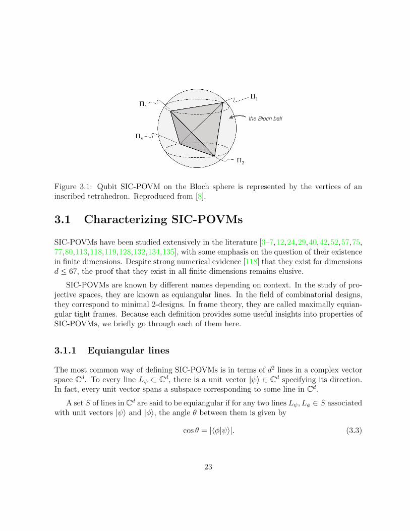
Figure 3.1: Qubit SIC-POVM on the Bloch sphere is represented by the vertices of aninscribed tetrahedron. Reproduced from [8].

3.1 Characterizing SIC-POVMs

SIC-POVMs have been studied extensively in the literature [3–7,12,24,29,40,42,52,57,75,77,80,113,118,119,128,132,134,135], with some emphasis on the question of their existencein finite dimensions. Despite strong numerical evidence [118] that they exist for dimensionsd ≤ 67, the proof that they exist in all finite dimensions remains elusive.

SIC-POVMs are known by different names depending on context. In the study of pro-jective spaces, they are known as equiangular lines. In the field of combinatorial designs,they correspond to minimal 2-designs. In frame theory, they are called maximally equian-gular tight frames. Because each definition provides some useful insights into properties ofSIC-POVMs, we briefly go through each of them here.

3.1.1 Equiangular lines

The most common way of defining SIC-POVMs is in terms of d2 lines in a complex vectorspace Cd. To every line Lψ ⊂ Cd, there is a unit vector |ψ〉 ∈ Cd specifying its direction.In fact, every unit vector spans a subspace corresponding to some line in Cd.

A set S of lines in Cd are said to be equiangular if for any two lines Lψ, Lφ ∈ S associatedwith unit vectors |ψ〉 and |φ〉, the angle θ between them is given by

cos θ = |〈φ|ψ〉|. (3.3)

23

Infinitely many vectors specify the same line because |ψ〉 and eiα |ψ〉 , α ∈ R span the samesubspace. However, the projection operator describing each line is unique since

Pψ =(eiα |ψ〉

) (e−iα〈ψ|

)= |ψ〉〈ψ|. (3.4)

In Cd, the maximal number of lines that are equiangular is obtained by assigningprojection operators to each line and demonstrating that those unit vectors are linearlyindependent. Since the lines in Cd are determined from the corresponding projectionoperators, then the space of interest is really the space of d × d Hermitian matrices towhich the projections belong to, viewed here as a real vector space of dimension d2.

Let Πi be the projection operator associated with line Lψi . Since Πi = |ψi〉〈ψi|, weknow that Tr (Πi) = 1 and Tr (ΠiΠj) = k ≤ 1. Now suppose there is a set {ci} such that∑

i

ciΠi = 0. (3.5)

If we take the trace on both sides, we get∑

i ci = 0. We can also multiply both sides ofEq. (3.5) by Πj and take the trace to obtain∑

i

ciTr (ΠiΠj) = cj +∑i 6=j

kci (3.6)

for any choice of j. Thus, ci = 0 for all i and the projectors Πi must be linearly independent.Since the projections belong to a vector space of dimension d2, this puts a bound on thesize of a set of equiangular lines.

Theorem 3.1.1. A set of equiangular lines in Cd has at most d2 elements.

Let L be a set of d2 equiangular lines in Cd. If we consider

I =∑i

ciΠi, (3.7)

taking the trace of both sides yields

Tr (I) = d =∑i

ci. (3.8)

Likewise, we can multiply Eq. (3.7) by Πj throughout before taking the trace to obtain

Tr (Πj) = 1 = cj +∑i 6=j

kci. (3.9)

24

Multiplying Eq. (3.8) by k and subtracting Eq. (3.9) from it gives cj(k − 1) = dk − 1 forall j, which then implies that

cj =1

dand k =

1

d+ 1. (3.10)

3.1.2 Complex projective design

An alternative way to define SIC-POVMs is to consider a particular structure in combi-natorial design theory called a t-design. A finite set X of points on a d-dimensional unithypersphere Sd is called a spherical t-design if the mean value of any polynomial of degreet or less on the discrete set X equals the mean value of the polynomial over the entiresphere. In other words,

1

|X|∑x∈X

f(x) =1

V

∫Sddy f(y) (3.11)

where V denotes the measure or volume of Sd. In practice, this means that we can ap-proximate an integral over a sphere numerically by a suitable choice of equally weighted|X| points.

The application to quantum mechanics takes the average over pure quantum statesrepresented by points in a complex projective space. Thus, a set S = {|ψi〉 ∈ H}ni=1 iscalled a complex projective t-design if

1

|S|

n∑i=1

|ψi〉〈ψi|⊗t =

∫CPd−1

dµ(φ) |φ〉〈φ|⊗t (3.12)

where µ is the unitarily invariant Haar measure.

Let Ht = ⊗tH be the t-fold tensor product of Hilbert spaces H and consider theoperator

St =n∑i=1

|Ψ(t)i 〉〈Ψ

(t)i |,

∣∣∣Ψ(t)i

⟩= |ψi〉⊗t . (3.13)

The set S forms a complex projective t-design if and only if

Tr(S2t

)=∑i,j

|〈ψi|ψj〉|2t =n2t!(d− 1)!

(t+ d− 1)!(3.14)

25

with n ≥ t+d−1Cd−1, the lower bound being the dimension of the symmetric subspace ofHt. Thus, SIC-POVMs are called minimal 2-designs since for S corresponding to elementsof a SIC-POVM,

Tr(S2

2

)=∑i,j

|〈ψi|ψj〉|4 =2d3

d+ 1(3.15)

where minimal refers to the fact that they achieve the lower bound on the size of S for2-designs, |S| ≥ d2. All 2-designs with |S| = d2 are necessarily equivalent to sets ofequiangular lines and therefore correspond to SIC-POVMs.

3.1.3 Maximal equiangular tight frame

A third way to characterize SIC-POVMs is through the notion of a frame, which generalizesthe notion of a basis. We know that any linearly independent set of vectors that span theentire vector space can serve as a basis for that space. In particular, the vectors in thebasis do not have to be orthogonal. Generally, this leads to a biorthogonal system for basisE and F : for every vector |ei〉 ∈ E, there is a dual vector |fi〉 ∈ F such that

〈fi|ej〉 = δij. (3.16)

A frame extends this idea to representations that expand over a linearly dependent set.

Here we are interested in the case of frames for the space of Hermitian operators H(H)on a Hilbert space of dimension d. Defining the inner product to be

〈A,B〉 = Tr (AB) (3.17)

for any A,B ∈ H(H), we see that H(H) is itself a real Hilbert space of dimension d2.

A frame F for H(H) is a set of operators F (λ) ∈ F that satisfy

a‖A‖2 ≤∫

Λ

dλ | 〈f(λ), A〉 |2 ≤ b‖B‖2 (3.18)

for all A ∈ H(H) and some 0 < a ≤ b. Observe that for an orthogonal basis {Bk},d2∑k=1

| 〈Bk, A〉 |2 = ‖A‖2 (3.19)

for all A ∈ H(H). A frame D = {D(λ)} is said to be dual to F if

A =

∫Λ

dλ 〈F (λ), A〉D(λ) (3.20)

26

for all A ∈ H(H).

Define the frame operator

S(A) =

∫Λ

dλ 〈F (λ), A〉F (λ), (3.21)

which is a superoperator acting on Hermitian operators. If S(A) = kA for some constantk, we say that F is a tight frame. From the frame operator, we can construct a dual frameS−1(F) called the canonical dual frame of F , which is defined by

A = S−1[S(A)] =

∫Λ

dλ 〈F (λ), A〉S−1[F (λ)]. (3.22)

This means that canonical dual frame operators consists of operators proportional to theframe operators in F .

A SIC-POVM forms a maximally equiangular tight frame with frame operators

Fi =1

d|ψi〉〈ψi| (3.23)

and it has a unique canonical dual frame given by operators

Di = S−1(Fi) ≡ d(d+ 1)Fi − I. (3.24)

It is straightforward to check that 〈Di, Fj〉 = δij. The equiangular condition means thatthe frame operators satisfy

〈Fi, Fj〉 =dδij + 1

d2(d+ 1). (3.25)

Chris Ferrie and Joseph Emerson [37] note that a SIC-POVM yields a frame representationfor finite-dimensional Hilbert spaces where states are represented by the frame operatorsvia the density operator reconstruction formula

ρ =∑i

〈Fi, ρ〉Di =∑i

〈Fi, ρ〉 [d(d+ 1)Fi − 1] (3.26)

where p(i) = 〈Fi, ρ〉 is a true probability and measurements are represented by dual frameoperators via the total probability law

Pr(k) =∑j

〈Fj, ρ〉 〈Dj, Ek〉 (3.27)

where we think of 〈Dj, Ek〉 as something like a conditional probability. It is however not atrue conditional probability since it is sometimes negative.

27

3.2 Weyl-Heisenberg SICs and the Clifford group

The conventional way to make a SIC-POVM is to find a set of d2 vectors |ψi〉 ∈ Hd suchthat

|〈ψi|ψj〉|2 =dδij + 1

d+ 1(3.28)

in which case the SIC-POVM elements are obtained from rescaling the rank-1 projectors

Πi = |ψi〉〈ψi|, i = 1, 2, . . . , d2. (3.29)

It is generally more convenient to think of a SIC-POVM in terms of these rank-1 projectorsbecause Tr (Πi) = 1. Thus, we distinguish the set {Πi}d

2

i=1 from a SIC-POVM by calling ita SIC set, or just SIC for short.

All SICs constructed to date have a group covariance property. Let G be a finite groupwith d2 elements and g 7→ G be a projective representation of G on the Hilbert space Hd,i.e., we consider an injective map g 7→ Ug where Ug is a d-dimensional unitary operatorsuch that for all g, h ∈ G,

UgUh = eiφghUgh, (3.30)

where eiφgh is just some overall phase.

Take some |ψ〉 ∈ Hd. If the set of vectors Ug |ψ〉 generates a SIC, we say that thecorresponding SIC is covariant with respect to the group G. In almost all known examples,there is just a single group used to construct SICs and is called the Weyl-Heisenberg group.

To describe the group, let {|j〉}dj=1 be an orthonormal basis for Cd. Introduce a pair ofoperators called the shift operator X and phase operator Z, defined as follows:

X |j〉 = |j ⊕ 1〉 ,Z |j〉 = ωj |j〉 , (3.31)

where ⊕ indicates addition modulo d and ω = e2πid . Now consider p = (p1, p2) ∈ Z2

d, thatis, p1, p2 = 0, 1, ..., d−1. It may be worth mentioning here that p corresponds to a point onthe discrete phase space of a finite-dimensional quantum system as described by WilliamWootters [131]. The vectors p allow us to define the displacement operator

Dp = τ p1p2Xp1Zp2 (3.32)

where τ = −eiπd . If we can find a suitable seed vector |ψ〉 such that |〈ψ|Dp |ψ〉 |2 = 1d+1

for~p 6= (0, 0), then the projectors

Πp = Dp|ψ〉〈ψ|D†p (3.33)

28

form a SIC of dimension d. The seed vector |ψ〉 is known as a fiducial vector.

Two key properties of displacement operators are:

D†p = D−p,

DpDq = τ 〈p,q〉Dp+q, (3.34)

where 〈p,q〉 = p2q1 − p1q2 is called the symplectic form.

The set of operators

W (d) ={τ rDp | r = 0, 1, ..., d− 1,p ∈ Z2

d

}(3.35)

is called the Weyl-Heisenberg group. Observe that while W (d) contains d3 elements, whenwe act its elements on a SIC fiducial, we only get d2 unique projectors, since vectors thatdiffer by an overall phase factor correspond to the same projection. The SIC generated byW (d) is called a Weyl-Heisenberg SIC.

We are also interested in the normalizer of the Weyl-Heisenberg group, called the Clif-ford group C(d) [3, 5, 53–55, 108], which is a subgroup of the set of unitary operators indimension d. If U ∈ C(d) then

UW (d)U † = W (d). (3.36)

If the set of anti-unitary operators that map W (d) to itself are added to the unitaries, weget a set called the extended Clifford group.

Marcus Appleby introduced a convenient way to parameterize the Clifford unitaries interms of symplectic matrices [3]. If we just consider the simpler case when d is odd, letSL(2,Zd) be the group of 2× 2 symplectic matrices with elements

F =

(α β

γ δ

)(3.37)

such that α, β, γ, δ ∈ Zd and det(F ) = 1 mod d. If the multiplicative inverse β−1 of βexists in Zd then we can construct the Clifford unitary

UF =1√d

d−1∑r,s=0

τβ−1(r2δ−2rs+s2α) |r〉 〈s|. (3.38)

such thatUFDpU

†F = DFp. (3.39)

29

If β−1 does not exist, one can look for some integer x such that α + xβ is nonzero andGCD(δ + xβ, d) = 1, then F = F1F2 where [3]

F1 =

(0 −1

1 x

), F2 =

(γ + xα δ + xβ

−α −β

)(3.40)

and UF1 and UF2 can be constructed as before. UF and UF1UF2 give the same Cliffordunitary up to a phase factor.

A particularly important symplectic matrix for finding SICs is given by

FZ =

(0 −1

1 −1

)(3.41)

and its corresponding Clifford unitary UFZ . We shall call FZ the Zauner matrix. Notethat the Zauner matrix can be defined in any finite dimension. According to a conjectureby Gerhard Zauner [134] and Marcus Appleby [3], there exists a SIC fiducial vector inevery dimension which is an eigenvector of UFZ , a unproven claim that is supported byall available numerical results to date. In Sec. 3.5, we will see that the Zauner matrix ind = 3 plays a prominent role in the linear dependencies of qutrit SICs.

3.3 Classifying qutrit SICs into inequivalent families

Since we are ultimately interested in the geometric features of quantum state space indimension three, we begin by examining the properties of qutrit SICs. All known SICs ind = 3 are Weyl-Heisenberg SICs, of which there are infinitely many.

Using the displacement operators in Eq. (3.32), a fiducial vector |ψ〉 generates a SICwith elements

Πp = Dp|ψ〉〈ψ|D†p. (3.42)

where the index p = (a, b) specifies the powers for the X and Z operators, respectively. Inthis case, it is useful to adopt the following convention for labeling the SIC elements:

1 : |ψ〉 2 : Z |ψ〉 3 : Z2 |ψ〉4 : X |ψ〉 5 : XZ |ψ〉 6 : XZ2 |ψ〉7 : X2 |ψ〉 8 : X2Z |ψ〉 9 : X2Z2 |ψ〉

(3.43)

30

where the SIC elements are given by projectors associated with each unit vector. Forexample, Π5 = XZ|ψ〉〈ψ|Z†X†.

Consider the continuous 1-parameter family of qutrit SIC fiducial vectors given by

|ψt〉 =

0

1

e2it

. (3.44)

Marcus Appleby [3] has shown that there are 3 types of orbits of the extended Cliffordgroup in d = 3 for which |ψ(t)〉 is in the orbit: a generic type corresponding to t ∈ (0, π

6)

and two exceptional ones corresponding to the endpoints t = 0, π6. Each orbit of the Clifford

group determines a set of fiducial vectors from which a number of distinct SICs can beidentified. For example, in the generic case, the orbit consists of 72 fiducials, forming 8distinct SICs for any fixed choice of 0 < t < π

6.

An important property of SICs on different orbits of the Clifford group is that generally,they are not related to one another by a unitary transformation. This makes it convenientfor us to classify qutrit SICs into 8 inequivalent SIC-families represented by the followingfiducial vectors:

∣∣∣ψ(0±)t

⟩=

1√2

0

e∓it

−e±it

,∣∣∣ψ(1±)

t

⟩=

√2

3

ω sin t

sin(t± 2π

3

)sin(t∓ 2π

3

) ,

∣∣∣ψ(2±)t

⟩=

√2

3

ω2 sin t

sin(t± 2π

3

)sin(t∓ 2π

3

) ,

∣∣∣ψ(3±)t

⟩=

√2

3

sin t

sin(t± 2π

3

)sin(t∓ 2π

3

) , (3.45)

where ω = ei2π3 and 0 ≤ t ≤ π

6. In this parametrization, the exceptional types correspond

to t = 0, where all 8 fiducials correspond to the same SIC, and t = π6, where there are 4

distinct SICs.

The unique SIC for t = 0 is generated by the SIC fiducial

|ψ0〉 =1√2

0

1

−1

. (3.46)

31

We will see that this particular SIC possesses nice properties that make it the simplest oneto consider when studying the probabilities obtained from qutrit SICs. In anticipation ofits important role for the remainder of this thesis, we refer to it as the most exceptionalSIC.

The only other exceptional case for which we have less than 8 SICs is when t = π6,

where there are 4 distinct SICs, whose fiducial vectors may be chosen as

∣∣∣ψ(0)π6

⟩=

1√2

0

1

1

,∣∣∣ψ(1)

π6

⟩=

1√6

ω

1

−2

,

∣∣∣ψ(2)π6

⟩=

1√6

ω2

1

−2

,∣∣∣ψ(3)

π6

⟩=

1√6

1

1

−2

. (3.47)

It is worth mentioning here that the SIC-families of Eq. (3.45) are inequivalent withrespect to Clifford unitaries; however, some of the SIC-families for different values of theparameter t are still related by a unitary operator that does not belong to the Cliffordgroup. Specifically, Huangjun Zhu [135] has shown that the SIC-families for t, π

9− t and

π9+t are, in fact, unitarily equivalent to each other, with the unitary transformation relating

them beingU = diag(1, s, s2), s = e−i

2π9 . (3.48)

Moreover, there are no other unitary equivalences. This means that every pair of SICs onany two different orbits corresponding to t ∈

[0, π

18

]are not equivalent.

3.4 Geometric invariants of qutrit SICs

Every SIC is fully characterized by two sets of geometrically invariant quantities: the firstset consist of numbers Tijk that give the trace of the product of every 3 SIC elements andare called triple products, i.e.,

Tijk = Tr (ΠiΠjΠk) . (3.49)

The other set is composed of the expansion coefficients Sijk of operator multiplicationbetween SIC elements when expressed in the basis defined by SIC projectors and are called

32

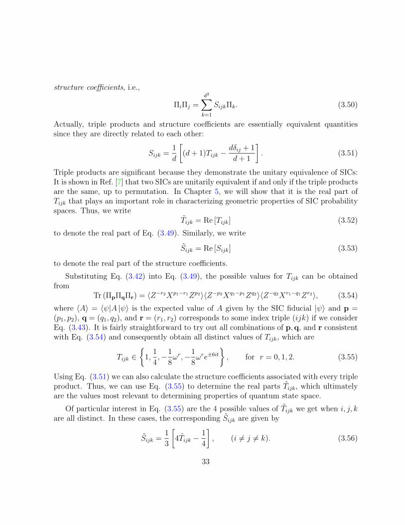
structure coefficients, i.e.,

ΠiΠj =d2∑k=1

SijkΠk. (3.50)

Actually, triple products and structure coefficients are essentially equivalent quantitiessince they are directly related to each other:

Sijk =1

d

[(d+ 1)Tijk −

dδij + 1

d+ 1

]. (3.51)

Triple products are significant because they demonstrate the unitary equivalence of SICs:It is shown in Ref. [7] that two SICs are unitarily equivalent if and only if the triple productsare the same, up to permutation. In Chapter 5, we will show that it is the real part ofTijk that plays an important role in characterizing geometric properties of SIC probabilityspaces. Thus, we write

Tijk = Re [Tijk] (3.52)

to denote the real part of Eq. (3.49). Similarly, we write

Sijk = Re [Sijk] (3.53)

to denote the real part of the structure coefficients.

Substituting Eq. (3.42) into Eq. (3.49), the possible values for Tijk can be obtainedfrom

Tr (ΠpΠqΠr) = 〈Z−r2Xp1−r1Zp2〉〈Z−p2Xq1−p1Zq2〉〈Z−q2Xr1−q1Zr2〉, (3.54)

where 〈A〉 = 〈ψ|A |ψ〉 is the expected value of A given by the SIC fiducial |ψ〉 and p =(p1, p2), q = (q1, q2), and r = (r1, r2) corresponds to some index triple (ijk) if we considerEq. (3.43). It is fairly straightforward to try out all combinations of p,q, and r consistentwith Eq. (3.54) and consequently obtain all distinct values of Tijk, which are

Tijk ∈{

1,1

4,−1

8ωr,−1

8ωre±6it

}, for r = 0, 1, 2. (3.55)

Using Eq. (3.51) we can also calculate the structure coefficients associated with every tripleproduct. Thus, we can use Eq. (3.55) to determine the real parts Tijk, which ultimatelyare the values most relevant to determining properties of quantum state space.

Of particular interest in Eq. (3.55) are the 4 possible values of Tijk we get when i, j, kare all distinct. In these cases, the corresponding Sijk are given by

Sijk =1

3

[4Tijk −

1

4

], (i 6= j 6= k). (3.56)

33

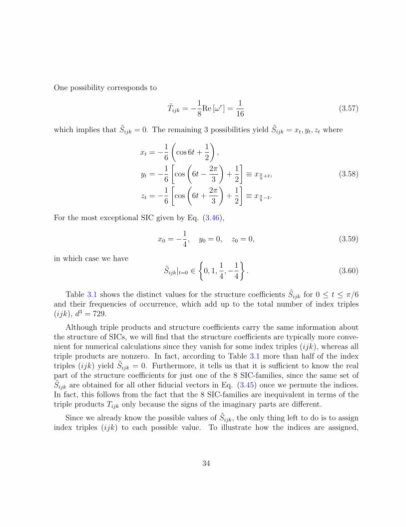
One possibility corresponds to

Tijk = −1

8Re [ωr] =

1

16(3.57)

which implies that Sijk = 0. The remaining 3 possibilities yield Sijk = xt, yt, zt where

xt = −1

6

(cos 6t+

1

2

),

yt = −1

6

[cos

(6t− 2π

3

)+

1

2

]≡ xπ

9+t, (3.58)

zt = −1

6

[cos

(6t+

2π

3

)+

1

2

]≡ xπ

9−t.

For the most exceptional SIC given by Eq. (3.46),

x0 = −1

4, y0 = 0, z0 = 0, (3.59)

in which case we have

Sijk|t=0 ∈{

0, 1,1

4,−1

4

}. (3.60)

Table 3.1 shows the distinct values for the structure coefficients Sijk for 0 ≤ t ≤ π/6and their frequencies of occurrence, which add up to the total number of index triples(ijk), d3 = 729.

Although triple products and structure coefficients carry the same information aboutthe structure of SICs, we will find that the structure coefficients are typically more conve-nient for numerical calculations since they vanish for some index triples (ijk), whereas alltriple products are nonzero. In fact, according to Table 3.1 more than half of the indextriples (ijk) yield Sijk = 0. Furthermore, it tells us that it is sufficient to know the realpart of the structure coefficients for just one of the 8 SIC-families, since the same set ofSijk are obtained for all other fiducial vectors in Eq. (3.45) once we permute the indices.In fact, this follows from the fact that the 8 SIC-families are inequivalent in terms of thetriple products Tijk only because the signs of the imaginary parts are different.

Since we already know the possible values of Sijk, the only thing left to do is to assignindex triples (ijk) to each possible value. To illustrate how the indices are assigned,

34

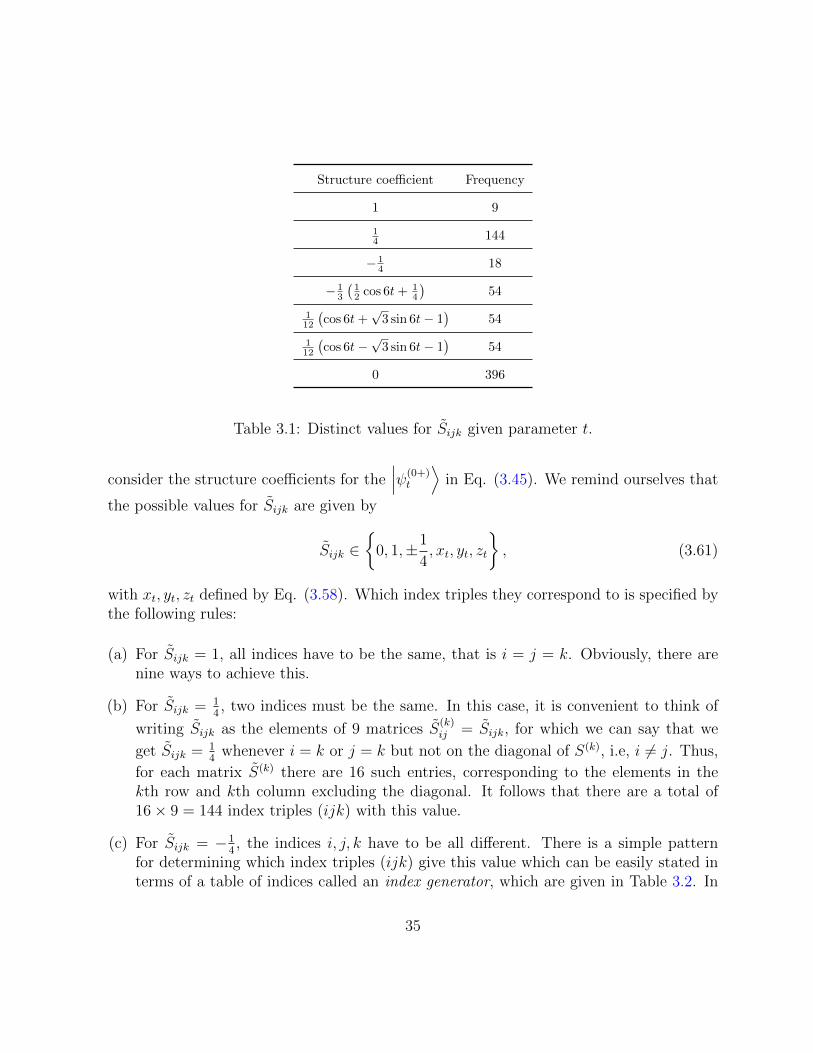
Structure coefficient Frequency

1 9

14 144

− 14 18

− 13

(12 cos 6t+ 1

4

)54

112

(cos 6t+

√3 sin 6t− 1

)54

112

(cos 6t−

√3 sin 6t− 1

)54

0 396

Table 3.1: Distinct values for Sijk given parameter t.

consider the structure coefficients for the∣∣∣ψ(0+)

t

⟩in Eq. (3.45). We remind ourselves that

the possible values for Sijk are given by

Sijk ∈{

0, 1,±1

4, xt, yt, zt

}, (3.61)

with xt, yt, zt defined by Eq. (3.58). Which index triples they correspond to is specified bythe following rules:

(a) For Sijk = 1, all indices have to be the same, that is i = j = k. Obviously, there arenine ways to achieve this.

(b) For Sijk = 14, two indices must be the same. In this case, it is convenient to think of

writing Sijk as the elements of 9 matrices S(k)ij = Sijk, for which we can say that we

get Sijk = 14

whenever i = k or j = k but not on the diagonal of S(k), i.e, i 6= j. Thus,

for each matrix S(k) there are 16 such entries, corresponding to the elements in thekth row and kth column excluding the diagonal. It follows that there are a total of16× 9 = 144 index triples (ijk) with this value.

(c) For Sijk = −14, the indices i, j, k have to be all different. There is a simple pattern

for determining which index triples (ijk) give this value which can be easily stated interms of a table of indices called an index generator, which are given in Table 3.2. In

35

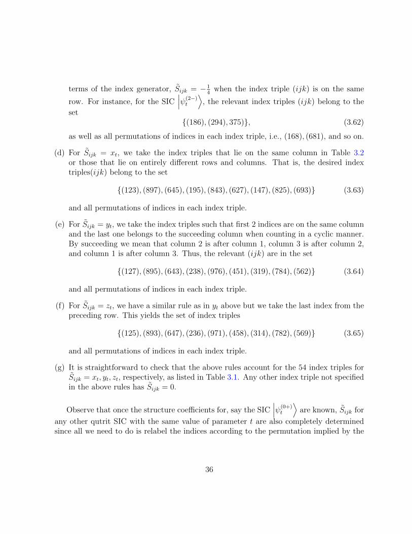
terms of the index generator, Sijk = −14

when the index triple (ijk) is on the same

row. For instance, for the SIC∣∣∣ψ(2−)

t

⟩, the relevant index triples (ijk) belong to the

set{(186), (294), 375)}, (3.62)

as well as all permutations of indices in each index triple, i.e., (168), (681), and so on.

(d) For Sijk = xt, we take the index triples that lie on the same column in Table 3.2or those that lie on entirely different rows and columns. That is, the desired indextriples(ijk) belong to the set

{(123), (897), (645), (195), (843), (627), (147), (825), (693)} (3.63)

and all permutations of indices in each index triple.

(e) For Sijk = yt, we take the index triples such that first 2 indices are on the same columnand the last one belongs to the succeeding column when counting in a cyclic manner.By succeeding we mean that column 2 is after column 1, column 3 is after column 2,and column 1 is after column 3. Thus, the relevant (ijk) are in the set

{(127), (895), (643), (238), (976), (451), (319), (784), (562)} (3.64)

and all permutations of indices in each index triple.

(f) For Sijk = zt, we have a similar rule as in yt above but we take the last index from thepreceding row. This yields the set of index triples

{(125), (893), (647), (236), (971), (458), (314), (782), (569)} (3.65)

and all permutations of indices in each index triple.

(g) It is straightforward to check that the above rules account for the 54 index triples forSijk = xt, yt, zt, respectively, as listed in Table 3.1. Any other index triple not specifiedin the above rules has Sijk = 0.

Observe that once the structure coefficients for, say the SIC∣∣∣ψ(0+)

t

⟩are known, Sijk for

any other qutrit SIC with the same value of parameter t are also completely determinedsince all we need to do is relabel the indices according to the permutation implied by the

36

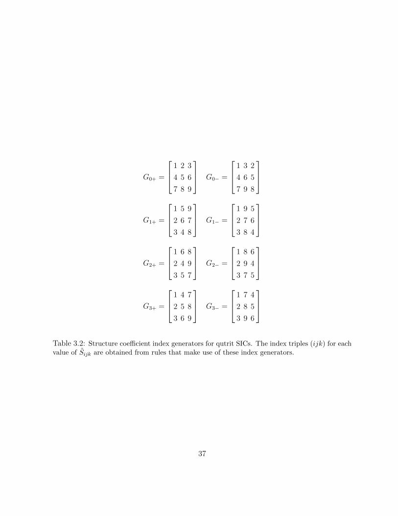
G0+ =

1 2 3

4 5 6

7 8 9

G0− =

1 3 2

4 6 5

7 9 8

G1+ =

1 5 9

2 6 7

3 4 8

G1− =

1 9 5

2 7 6

3 8 4

G2+ =

1 6 8

2 4 9

3 5 7

G2− =

1 8 6

2 9 4

3 7 5

G3+ =

1 4 7

2 5 8

3 6 9

G3− =

1 7 4

2 8 5

3 9 6

Table 3.2: Structure coefficient index generators for qutrit SICs. The index triples (ijk) for eachvalue of Sijk are obtained from rules that make use of these index generators.

37

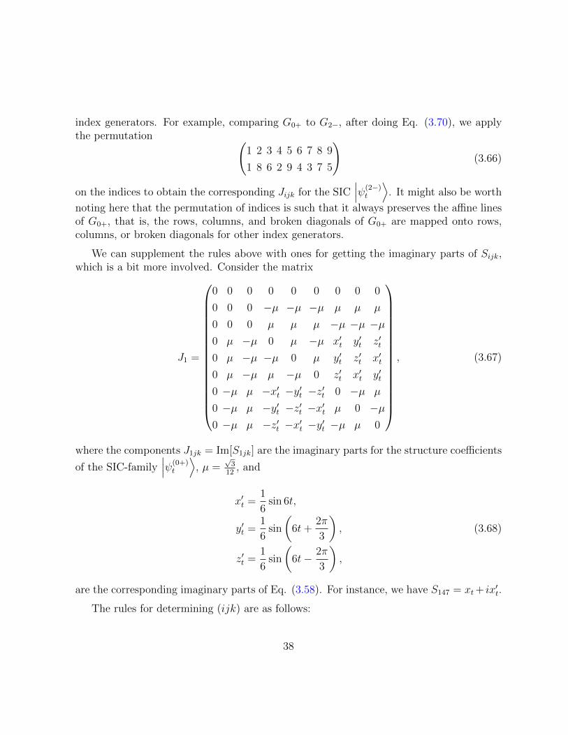
index generators. For example, comparing G0+ to G2−, after doing Eq. (3.70), we applythe permutation (

1 2 3 4 5 6 7 8 9

1 8 6 2 9 4 3 7 5

)(3.66)

on the indices to obtain the corresponding Jijk for the SIC∣∣∣ψ(2−)

t

⟩. It might also be worth

noting here that the permutation of indices is such that it always preserves the affine linesof G0+, that is, the rows, columns, and broken diagonals of G0+ are mapped onto rows,columns, or broken diagonals for other index generators.

We can supplement the rules above with ones for getting the imaginary parts of Sijk,which is a bit more involved. Consider the matrix

J1 =

0 0 0 0 0 0 0 0 0

0 0 0 −µ −µ −µ µ µ µ

0 0 0 µ µ µ −µ −µ −µ0 µ −µ 0 µ −µ x′t y′t z′t

0 µ −µ −µ 0 µ y′t z′t x′t

0 µ −µ µ −µ 0 z′t x′t y′t

0 −µ µ −x′t −y′t −z′t 0 −µ µ

0 −µ µ −y′t −z′t −x′t µ 0 −µ0 −µ µ −z′t −x′t −y′t −µ µ 0

, (3.67)

where the components J1jk = Im[S1jk] are the imaginary parts for the structure coefficients

of the SIC-family∣∣∣ψ(0+)

t

⟩, µ =

√3

12, and

x′t =1

6sin 6t,

y′t =1

6sin

(6t+

2π

3

), (3.68)

z′t =1

6sin

(6t− 2π

3

),

are the corresponding imaginary parts of Eq. (3.58). For instance, we have S147 = xt+ ix′t.

The rules for determining (ijk) are as follows:

38

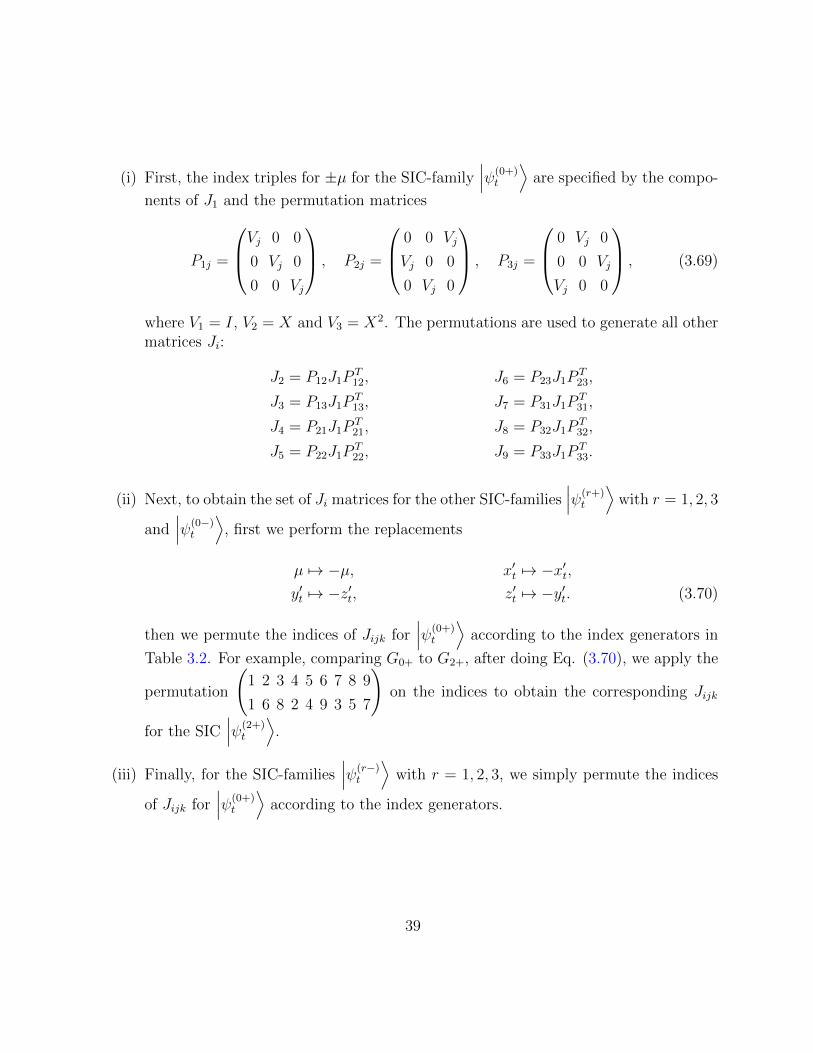
(i) First, the index triples for ±µ for the SIC-family∣∣∣ψ(0+)

t

⟩are specified by the compo-

nents of J1 and the permutation matrices

P1j =

Vj 0 0

0 Vj 0

0 0 Vj

, P2j =

0 0 Vj

Vj 0 0

0 Vj 0

, P3j =

0 Vj 0

0 0 Vj

Vj 0 0

, (3.69)

where V1 = I, V2 = X and V3 = X2. The permutations are used to generate all othermatrices Ji:

J2 = P12J1PT12, J6 = P23J1P

T23,

J3 = P13J1PT13, J7 = P31J1P

T31,

J4 = P21J1PT21, J8 = P32J1P

T32,

J5 = P22J1PT22, J9 = P33J1P

T33.

(ii) Next, to obtain the set of Ji matrices for the other SIC-families∣∣∣ψ(r+)

t

⟩with r = 1, 2, 3

and∣∣∣ψ(0−)

t

⟩, first we perform the replacements

µ 7→ −µ, x′t 7→ −x′t,y′t 7→ −z′t, z′t 7→ −y′t. (3.70)

then we permute the indices of Jijk for∣∣∣ψ(0+)

t

⟩according to the index generators in

Table 3.2. For example, comparing G0+ to G2+, after doing Eq. (3.70), we apply the

permutation

(1 2 3 4 5 6 7 8 9

1 6 8 2 4 9 3 5 7

)on the indices to obtain the corresponding Jijk

for the SIC∣∣∣ψ(2+)

t

⟩.

(iii) Finally, for the SIC-families∣∣∣ψ(r−)

t

⟩with r = 1, 2, 3, we simply permute the indices

of Jijk for∣∣∣ψ(0+)

t

⟩according to the index generators.

39

3.5 Linear dependency structure of qutrit SICs

We have already seen that by thinking in terms of a set of equiangular lines in a complexlinear space, a SIC can always be described with a set of vectors

S ={|ψj〉 ∈ Hd

∣∣∣ j = 1, 2, . . . , d2}

(3.71)

that define the 1-dimensional subspaces on which SIC elements project. Because the num-ber of vectors in such a set is much larger than the number of dimensions, they are certainlylinearly dependent. However, we may ask if choosing any d vectors from the set S spansthe entire Hilbert space. That is, does every subset of d vectors from S form a linearlyindependent set and a basis for Hd? It turns out that the answer to this question is neg-ative for d = 3. In fact, according to Hoan Dang, et al., such linearly dependent subsetscan always be found for SICs in dimensions divisible by 3 [30]. In this section, we describesuch a linear dependency structure for qutrit SICs.

We begin with some definitions:

Definition 3.5.1. A p-vector is any 2-element vector

p =

(a

b

)(3.72)

where a, b = 0, 1, . . . , d− 1 so that each p corresponds to a displacement operator Dp.

Definition 3.5.2. A p-set is any set of d p-vectors

{p1,p2, . . . ,pd}. (3.73)

If pi =

(ai

bi

)for i = 1, 2, ..., d, we will write the corresponding p-set in shorthand notation

as(a1b1, a2b2, ..., adbd). (3.74)

Definition 3.5.3. In dimension 3, the set of three p-vectors (p1,p2,p3) is called a goodp-set whenever the corresponding set of vectors

{Dp1 |ψ〉 , Dp2 |ψ〉 , Dp3 |ψ〉} (3.75)

form a linearly dependent set for some fiducial vector |ψ〉.

40

For the 8 SIC-families listed by Eq. (3.45), we obtain three good p-sets for each SIC-family if we take the following p-sets:∣∣∣ψ(0±)

t

⟩: (00, 01, 02), (10, 11, 12), (20, 21, 22),∣∣∣ψ(1±)

t

⟩: (00, 12, 21), (01, 10, 22), (02, 11, 20),∣∣∣ψ(2±)

t

⟩: (00, 11, 22), (01, 12, 20), (02, 10, 21),∣∣∣ψ(3±)

t

⟩: (00, 10, 20), (01, 11, 21), (02, 12, 22). (3.76)

where for instance, each p-set for∣∣∣ψ(0±)

t

⟩corresponds to the rows of

G0+ =

00 01 02

10 11 12

20 21 22

(3.77)

which can be identified with the index generator G0+ in Table 3.2 if we apply our labelingconventions in Eq. (3.43). In fact, one can check from the rules for specifying the indextriples (ijk) of the structure coefficients described in Sec. 3.4 that the good p-sets of Eq.(3.76) for each SIC-family correspond to index triples (ijk) such that Sijk = −1

4, that is,

the rows of the index generators in Table 3.2.

Something more interesting happens when we consider a few special cases, specificallythe linear dependencies for the most exceptional SIC given by t = 0 and the 8 SICscorresponding to t = π

9(which are equivalent to each other and related by the unitary

matrix given by Eq. (3.48).) Again, in terms of p-vectors, we obtain linearly dependentsets of SIC-vectors with the fiducials in Eq. (3.45) for the following 12 good p-sets:

(00, 01, 02), (00, 11, 22), (00, 10, 20), (00, 12, 21),

(10, 11, 12), (01, 12, 20), (01, 11, 21), (01, 10, 22),

(20, 21, 22), (02, 10, 21), (02, 12, 22), (02, 11, 20),

(3.78)

which coincidentally is the union of all the p-sets in Eq. (3.76).

The linear dependency structure of the most exceptional SIC is described in detail inTable 3.3. The linear dependency condition specifies how the SIC-vectors corresponding tothe p-sets sum to zero and the orthogonal subspace is specified by a unit vector that spansthe 1-dimensional space. It is worth noting that every 3 consecutive orthogonal subspace

41

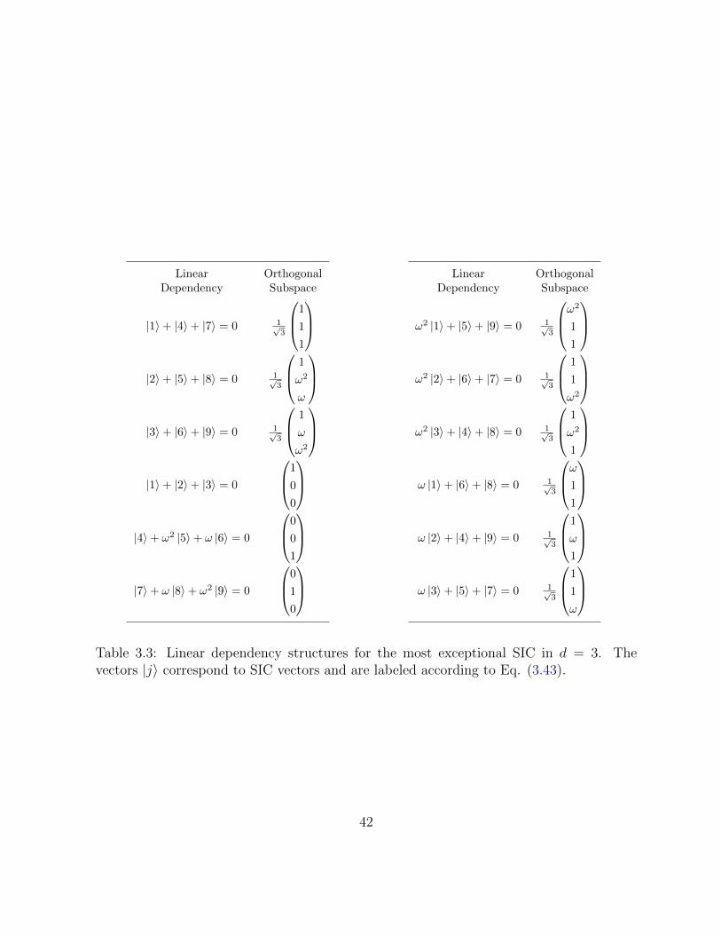
Linear OrthogonalDependency Subspace

|1〉+ |4〉+ |7〉 = 0 1√3

1

1

1

|2〉+ |5〉+ |8〉 = 0 1√

3

1

ω2

ω

|3〉+ |6〉+ |9〉 = 0 1√

3

1

ω

ω2

|1〉+ |2〉+ |3〉 = 0

1

0

0

|4〉+ ω2 |5〉+ ω |6〉 = 0

0

0

1

|7〉+ ω |8〉+ ω2 |9〉 = 0

0

1

0

Linear OrthogonalDependency Subspace

ω2 |1〉+ |5〉+ |9〉 = 0 1√3

ω2

1

1

ω2 |2〉+ |6〉+ |7〉 = 0 1√

3

1

1

ω2

ω2 |3〉+ |4〉+ |8〉 = 0 1√

3

1

ω2

1

ω |1〉+ |6〉+ |8〉 = 0 1√

3

ω11

ω |2〉+ |4〉+ |9〉 = 0 1√

3

1

ω

1

ω |3〉+ |5〉+ |7〉 = 0 1√

3

1

1

ω

Table 3.3: Linear dependency structures for the most exceptional SIC in d = 3. Thevectors |j〉 correspond to SIC vectors and are labeled according to Eq. (3.43).

42

vector as listed in Table 3.3 (1st to 3rd, 4th to 6th, etc.) form a basis for the 3-dimensionalHilbert space. Moreover, the four bases constitute a complete set of mutually unbiasedbases (MUBs) in d = 3.

Aside from the most exceptional SIC, there are 8 other SICs which also have 12 goodp-sets, those given by t = π

9. The good p-sets for these SICs are listed in Table 3.4. A key

difference between good p-sets of the most exceptional SIC and that of the 8 SICs witht = π

9is that for the most exceptional SIC, every good p-set has the property

3∑i=1

pi =

(0

0

)mod 3. (3.79)

This, however, is not the case for the 8 SICs with t = π9

since a quick glance at Table 3.4will show that only p-sets in the first column have this property.

Lane Hughston [65] showed that the linear dependency structure for the 9 SICs with 12good p-sets corresponds in projective geometry to structure known as a Hesse configuration.A Hesse configuration consists of a set of 12 lines and 9 points in a complex projectiveplane where the 9 points are the inflection points of a non-singular cubic function

P (x1, x2, x3) = x31 + x3

2 + x33 + tx1x2x3, t ∈ C (3.80)

such that every 3 inflection points fall on a line on the projective plane [64]. The inflectionpoints are given by points on the curve for which the determinant of the Hessian matrixof P vanishes, that is, if we take the matrix H with elements

Hij =∂2P

∂xi∂xj(3.81)

then we havedet(H) = (2t3 + 216)x1x2x3 − 6t2(x3

1 + x32 + x3

3) = 0. (3.82)

The inflection points coincide for all values of t and correspond to the most exceptional SICvectors. Moreover, the family of cubic polynomials defined by P (x1, x2, x3) has 4 singularmembers corresponding to t = 0 and the cube roots of t3 + 81 = 0, the resulting projectivelines form triangles whose vertices are given by the orthogonal subspace vectors in Table3.3 [15]. Because of this, we refer to the most exceptional SIC and the 8 SICs with t = π

9

as Hesse SICs.

43

For∣∣∣ψ(0+)

π9

⟩(00,01,02) (00,10,22) (00,11,21) (00,12,20)

(10,11,12) (01,11,20) (01,12,22) (01,10,21)

(20,21,22) (02,12,21) (02,10,20) (02,11,22)

For∣∣∣ψ(0−)

π9

⟩(00,01,02) (00,12,22) (00,10,21) (00,11,20)

(10,11,12) (01,10,20) (01,11,22) (01,12,21)

(20,21,22) (02,11,21) (02,12,20) (02,10,22)

For∣∣∣ψ(1+)

π9

⟩(00,11,22) (00,12,10) (00,20,02) (00,01,21)

(01,12,20) (11,20,21) (11,01,10) (11,12,02)

(02,10,21) (22,01,02) (22,12,21) (22,20,10)

For∣∣∣ψ(1−)

π9

⟩(00,11,22) (00,20,21) (00,12,02) (00,01,10)

(01,12,20) (11,01,02) (11,20,10) (11,12,21)

(02,10,21) (22,12,10) (22,01,21) (22,20,02)

For∣∣∣ψ(2+)

π9

⟩(00,12,21) (00,10,11) (00,02,22) (00,01,20)

(01,10,22) (12,22,20) (12,01,11) (12,10,02)

(02,11,20) (21,01,02) (21,10,20) (21,21,11)

For∣∣∣ψ(2−)

π9

⟩(00,12,21) (00,22,20) (00,10,02) (00,01,11)

(01,10,22) (12,01,02) (12,22,11) (12,10,20)

(02,11,20) (21,10,11) (21,01,20) (21,22,02)

For∣∣∣ψ(3+)

π9

⟩(00,10,20) (00,11,12) (00,21,02) (00,01,22)

(01,11,21) (10,21,22) (10,01,12) (10,11,02)

(02,12,22) (20,01,02) (20,11,22) (20,21,12)

For∣∣∣ψ(3−)

π9

⟩(00,10,20) (00,21,22) (00,11,02) (00,01,12)

(01,11,21) (10,01,02) (10,21,12) (10,11,22)

(02,12,22) (20,11,12) (20,01,22) (20,21,02)

Table 3.4: Good p-sets yielding linear dependencies for the 8 SICs with t = π9 .

44

3.6 The Zauner subspace for qutrit SICs

Recall that in Sec. 3.2, we mentioned that in the Clifford group for displacement operators,there is a symplectic unitary UFZ given by Eq. (3.38) that is generated from the Zaunermatrix FZ defined by Eq. (3.41). The significance of UFZ is that according to a conjectureby Gerhard Zauner, one of its eigenvectors is always a SIC fiducial [134], and existingnumerical evidence strongly supports this claim. In d = 3, the Zauner matrix is given by

FZ =

(0 2

1 2

)(3.83)

because −1 mod 3 = 2 and the corresponding Zauner unitary UFZ takes the form

UFZ =1√3eiπ6

2∑r,s=0

τ 2(2r2−2rs) |r〉 〈s| = 1√3eiπ6

2∑r,s=0

ω2r(r−s) |r〉 〈s|, (3.84)

where τ = −eiπ3 and τ 2 = ω. In the standard basis, we can write UFZ as

UFZ =eiπ6

√3

1 1 1

ω2 1 ω

ω2 ω 1

. (3.85)

In Zauner’s conjecture [3, 134], the eigenspace of interest is the largest subspace wherethe overall phase can be chosen so that it has a unit eigenvalue. We denote the Zaunersubspace by Z, which in d = 3 is given by

Z = span

−ω

2

0

1

,

−ω2

1

0

, (3.86)

where the span is over the complex field C.

In Sec 3.5, we saw that there are 9 qutrit SICs for which the number of good p-sets is 12:the most exceptional SIC and the 8 SICs generated with t = π

9. For any other SIC-family,

the number of good p-sets is 3. In this section, we want to answer the following questions:

(a) Are there any vectors in the Zauner subspace other than SIC fiducials that give rise tolinear dependencies?

45

(b) Do the Hesse SICs exhaust all SICs with a maximal number of linear dependencies ind = 3?

We will show that the answer is affirmative for both questions in d = 3.

Observe that any Zauner eigenvector |ψ〉 ∈ Z can be written as

|ψ〉 =

−ω2(x+ y)

y

x

, (3.87)

where x, y ∈ C. For each |ψ〉 ∈ Z, we associate a set P

P = {Dp |ψ〉 | p ∈ Z23}, (3.88)

where Dp are just the usual displacement operators defined by Eq. (3.32). As we havedone previously, because there is a one-to-one correspondence between P and all p-vectorsin Z2

3 (except when y = ωx), we can refer to vectors in P by their corresponding p-vectors.

It was mentioned in Sec. 3.5 that the p-sets

(00, 12, 21), (01, 10, 22), (02, 11, 20) (3.89)

are always good p-sets. This may be seen if we explicitly list down the set P generated byEq. (3.87):

P =

−ω2(x+ y)

y

x

,

x

−ω2(x+ y)

y

,

y

x

−ω2(x+ y)

,

−ω2(x+ y)

ωy

ω2x

,

x

−(x+ y)

ω2y

,

y

ωx

−ω(x+ y)

,

−ω2(x+ y)

ω2y

ωx

,

x

ω(x+ y)

ωy

,

y

ω2x

−(x+ y)

. (3.90)

The vectors of P are displayed so that each row matches exactly with the p-sets in Eq.(3.89).

46

The Hesse SICs are the only ones which maximize the number of good p-sets. Thisfollows from considering any of 3 SIC vectors that do not correspond to any p-set in Eq.(3.89) and setting the value of their determinant to zero [30]. Doing so gives∣∣∣∣∣∣∣

0 −e2itωy 1

1 0 e2itωz

−e2itωx 1 0

∣∣∣∣∣∣∣ = 1 + e6itωx+y+z = 0 (3.91)

which implies thatωr = e6it, r = 0, 1, 2. (3.92)

which holds if and only if t = 0 and t = π9, which are the Hesse SICs. Any other SIC with

12 good p-sets must then be unitarily equivalent to the Hesse SICs.

3.7 Lie algebraic properties of qutrit SICs

As we have mentioned before, our interest in SICs stems primarily from the fact that anarbitrary density operator can be expanded in terms of a SIC. However, Marcus Appleby,Steve Flammia, and Chris Fuchs [7] have shown that SICs can be used not just as a basisfor the space of Hermitian matrices, they also can serve as a basis for the space of allcomplex matrices of dimension d, that is, the Lie algebra gld(C).

If we take any linear operator B acting on some Hilbert space Hd, we can find a uniqueset of expansion coefficients bk such that

B =d2∑k=1

bkΠk. (3.93)

For the special case B = ΠiΠj the expansion coefficients bk correspond to the structurecoefficients Sijk. If we define the quantity

Jrst =d+ 1

d(Trst − T ∗rst) , (3.94)

then using Eq. (3.51), we may write

[Πr,Πs] =d2∑t=1

JrstΠt (3.95)

47

so that the Jrst are, in fact, the structure constants for the Lie algebra gld(C). Note thatthe Jrst are proportional to the imaginary part of the triple products.

It is not difficult to verify that the structure constants Jrst satisfy the properties of aLie algebra. In particular, they obey the Jacobi identity

d2∑q=1

(JrsqJtqu + JstqJrqu + JtrqJsqu) = 0, (3.96)

for all r, s, t, u = 1, ..., d2. It may be worth noting that the matrix Jr with elements

[Jr]st = Jrst (3.97)

is the adjoint representative of Πr in the basis formed by the SIC projectors, i.e.,

adΠrΠs = [Πr,Πs] =d2∑t=1

JrstΠt. (3.98)

An important property of the adjoint matrix Jr is that it has a spectral decompositionof the form

Jr = Qr −QTr (3.99)

where Qr is a rank-(d− 1) projector with the special property that

QrQTr = 0. (3.100)

We refer to this as the Q-QT property [7].

The relationship between the triple products and the projectors Qr is given by

Tr =d

d+ 1Qr +

2d

d+ 1|er〉〈er|, (3.101)

where the matrix Tr has elements (Tr)st = Trst and

|er〉 =

√d+ 1

2d

d2∑s=1

K2rs |s〉 , Krs =

√dδrs + 1

d+ 1, (3.102)

and the set {|s〉}d2

s=1 is the standard basis in dimension d2. Observe that the quantity Krs

is just the absolute value of the inner product between SIC vectors, that is, the elements

Grs = 〈ψr|ψs〉 = Krseiθrs (3.103)

48

of the Gram matrix of the SIC with vectors |ψr〉.

The Gram matrix satisfies an identity∑r

Gs1rGs2rGrt1Grt2 =d

d+ 1(Gs1t1Gs2t2Gs1t2Gs2t1) (3.104)

which follows from the 2-design property of SICs:∑r

Πr ⊗ Πr =2d

d+ 1Psym (3.105)

where Psym denotes the projector onto the symmetric subspace of Cd ⊗ Cd. The tripleproducts are related to the Gram matrix elements by

Trst = GrsGstGtr = KrsKstKtreiθrst (3.106)

whereθrst = θrs + θst + θtr. (3.107)

This shows that the most interesting features of the Gram matrix and the triple productsare already contained in the angle tensors θrs.

Using geometrical considerations of the Q-QT property, Appleby, Flammia, and Fuchsshowed that the existence of a SIC in dimension d is equivalent to the construction of ahighly symmetric basis for the Lie algebra gld(C) [7]. More specifically, let Lr be any set ofd2 Hermitian operators which form a basis for gld(C) and Cr be the adjoint representativeof Lr. Then the necessary and sufficient condition for Cr to be decomposable into

Cr = Qr −QTr (3.108)

where Qr is a rank d − 1 projector such that QrQTr = 0 is that there exists a SIC with

elements Πr such thatLr = εr (Πr + αI) (3.109)

for some fixed α ∈ R and εr = ±. Moreover, the existence of a Hermitian basis for gld(C)with a Q-QT property is necessary and sufficient for the existence of a SIC in dimension d.

To illustrate this, we can use Eq.(3.101) to calculate Qr from the triple products Tijk forqutrit SICs. In particular, we are interested in the Q-projectors for the most exceptional

49

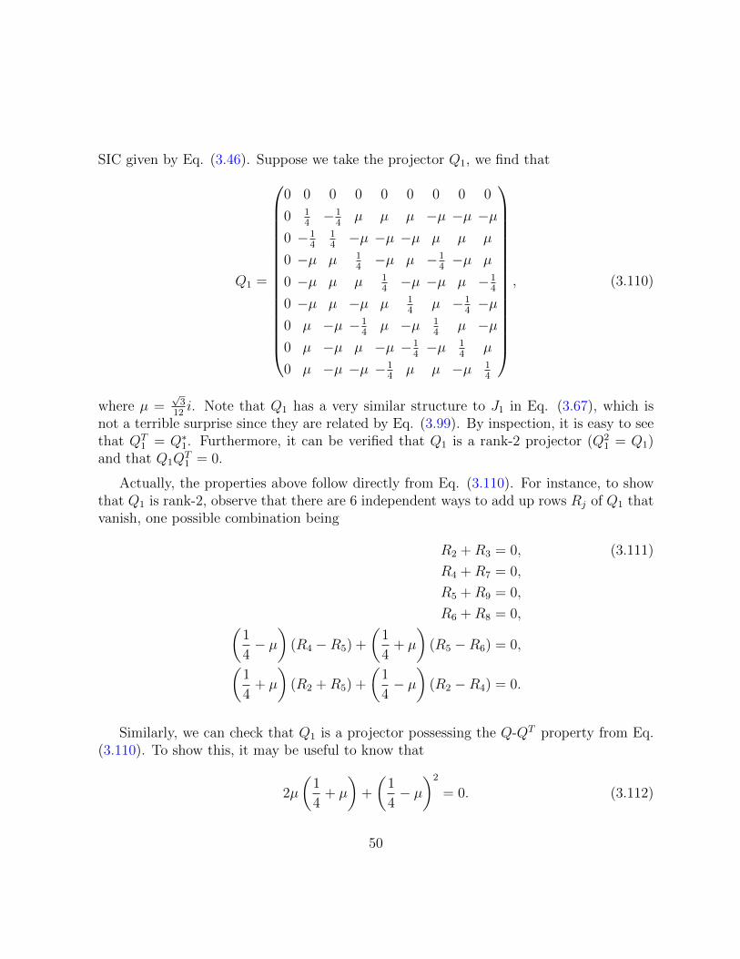
SIC given by Eq. (3.46). Suppose we take the projector Q1, we find that

Q1 =

0 0 0 0 0 0 0 0 0

0 14−1

4µ µ µ −µ −µ −µ

0 −14

14−µ −µ −µ µ µ µ

0 −µ µ 14−µ µ −1

4−µ µ

0 −µ µ µ 14−µ −µ µ −1

4

0 −µ µ −µ µ 14

µ −14−µ

0 µ −µ −14

µ −µ 14

µ −µ0 µ −µ µ −µ −1

4−µ 1

4µ

0 µ −µ −µ −14

µ µ −µ 14

, (3.110)

where µ =√

312i. Note that Q1 has a very similar structure to J1 in Eq. (3.67), which is

not a terrible surprise since they are related by Eq. (3.99). By inspection, it is easy to seethat QT

1 = Q∗1. Furthermore, it can be verified that Q1 is a rank-2 projector (Q21 = Q1)

and that Q1QT1 = 0.

Actually, the properties above follow directly from Eq. (3.110). For instance, to showthat Q1 is rank-2, observe that there are 6 independent ways to add up rows Rj of Q1 thatvanish, one possible combination being

R2 +R3 = 0, (3.111)

R4 +R7 = 0,

R5 +R9 = 0,

R6 +R8 = 0,(1

4− µ

)(R4 −R5) +

(1

4+ µ

)(R5 −R6) = 0,(

1

4+ µ

)(R2 +R5) +

(1

4− µ

)(R2 −R4) = 0.

Similarly, we can check that Q1 is a projector possessing the Q-QT property from Eq.(3.110). To show this, it may be useful to know that

2µ

(1

4+ µ

)+

(1

4− µ

)2

= 0. (3.112)

50

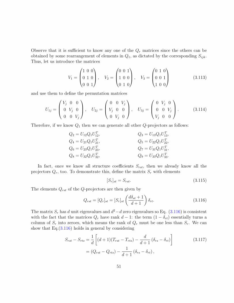
Observe that it is sufficient to know any one of the Qr matrices since the others can beobtained by some rearrangement of elements in Q1, as dictated by the corresponding Sijk.Thus, let us introduce the matrices

V1 =

1 0 0

0 1 0

0 0 1

, V2 =

0 0 1

1 0 0

0 1 0

, V3 =

0 1 0

0 0 1

1 0 0

(3.113)

and use them to define the permutation matrices

U1j =

Vj 0 0

0 Vj 0

0 0 Vj

, U2j =

0 0 Vj

Vj 0 0

0 Vj 0

, U3j =

0 Vj 0

0 0 Vj

Vj 0 0

. (3.114)

Therefore, if we know Q1 then we can generate all other Q-projectors as follows:

Q2 = U12Q1UT12, Q3 = U13Q1U

T13,

Q4 = U21Q1UT21, Q5 = U22Q1U

T22,

Q6 = U23Q1UT23, Q7 = U31Q1U

T31,

Q8 = U32Q1UT32, Q9 = U33Q1U

T33.

In fact, once we know all structure coefficients Srst, then we already know all theprojectors Qr, too. To demonstrate this, define the matrix Sr with elements

[Sr]st = Srst. (3.115)

The elements Qrst of the Q-projectors are then given by

Qrst = [Qr]st = [Sr]st

(dδst + 1

d+ 1

)δrt. (3.116)

The matrix Sr has d unit eigenvalues and d2−d zero eigenvalues so Eq. (3.116) is consistentwith the fact that the matrices Qr have rank d− 1: the term (1− δrt) essentially turns acolumn of Sr into zeroes, which means the rank of Qr must be one less than Sr. We canshow that Eq.(3.116) holds in general by considering

Srst − Srts =1

d

[(d+ 1)(Trst − Trts)−

d

d+ 1(δrs − δrt)

](3.117)

= (Qrst −Qrts)−1

d+ 1(δrs − δrt) ,

51

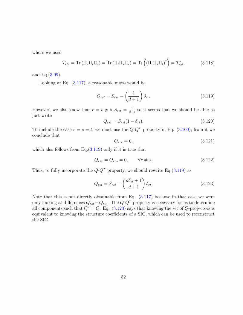
where we used

Trts = Tr (ΠrΠtΠs) = Tr (ΠtΠsΠr) = Tr(

(ΠrΠsΠt)†)

= T ∗rst, (3.118)

and Eq.(3.99).

Looking at Eq. (3.117), a reasonable guess would be

Qrst = Srst −(

1

d+ 1

)δrt. (3.119)

However, we also know that r = t 6= s, Srst = 1d+1

so it seems that we should be able tojust write

Qrst = Srst(1− δrt). (3.120)

To include the case r = s = t, we must use the Q-QT property in Eq. (3.100); from it weconclude that

Qrrr = 0, (3.121)

which also follows from Eq.(3.119) only if it is true that

Qrsr = Qrrs = 0, ∀r 6= s. (3.122)

Thus, to fully incorporate the Q-QT property, we should rewrite Eq.(3.119) as

Qrst = Srst −(dδst + 1

d+ 1

)δrt. (3.123)

Note that this is not directly obtainable from Eq. (3.117) because in that case we wereonly looking at differences Qrst−Qrts. The Q-QT property is necessary for us to determineall components such that Q2 = Q. Eq. (3.123) says that knowing the set of Q-projectors isequivalent to knowing the structure coefficients of a SIC, which can be used to reconstructthe SIC.

52

Chapter 4

Practical implementations ofSIC-POVMs

Quantum state tomography describes various methods for estimating the state of a quan-tum system from the statistics of a sufficiently informative set of measurements [67,103]. Itcontinues to be one of the primary challenges in quantum information and quantum com-puting since many quantum information processing tasks requires the ability to determinethe quantum state in a robust and efficient manner.

The state of an ensemble of d-dimensional quantum systems is typically described bya density operator, which in general is an abstract list of d2 numbers. This means that toperform tomography involves carrying out at least d2 linearly independent measurementsand then using one of a number of mathematical techniques to determine the state, suchas maximum likelihood estimation.

In practical quantum state tomography, SIC-POVMs are particularly important be-cause they are optimal according to the following fairly standard measures of efficiency:

(i) they use the minimal number of expectation values, leading to less redundancy andfaster convergence in state reconstruction, and

(ii) they achieve the smallest error probability with respect to Hilbert-Schmidt distancebetween the estimated and “true” density operator for the measured system [119].

Here we describe various methods for experimental SIC-POVMs, including two newproposals, one involving a storage loop with weak projections, while another involvingNaimark unitaries implemented with integrated optics.

53

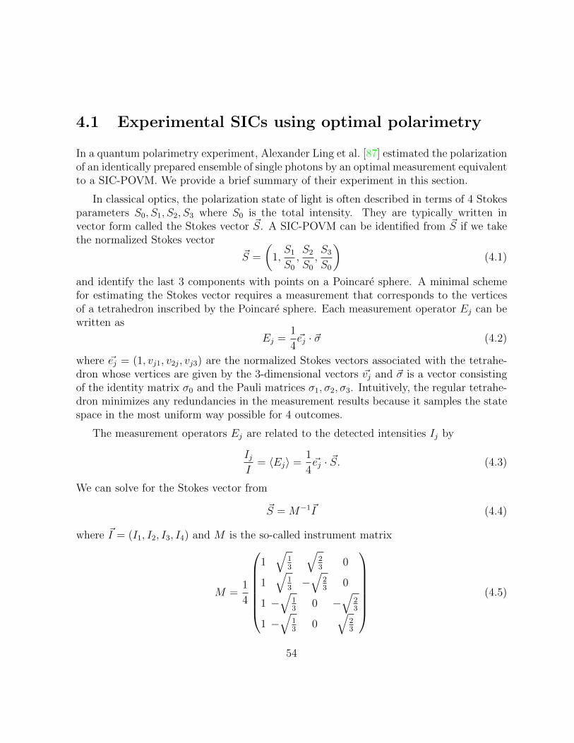
4.1 Experimental SICs using optimal polarimetry

In a quantum polarimetry experiment, Alexander Ling et al. [87] estimated the polarizationof an identically prepared ensemble of single photons by an optimal measurement equivalentto a SIC-POVM. We provide a brief summary of their experiment in this section.

In classical optics, the polarization state of light is often described in terms of 4 Stokesparameters S0, S1, S2, S3 where S0 is the total intensity. They are typically written invector form called the Stokes vector ~S. A SIC-POVM can be identified from ~S if we takethe normalized Stokes vector

~S =

(1,S1

S0

,S2

S0

,S3

S0

)(4.1)

and identify the last 3 components with points on a Poincare sphere. A minimal schemefor estimating the Stokes vector requires a measurement that corresponds to the verticesof a tetrahedron inscribed by the Poincare sphere. Each measurement operator Ej can bewritten as

Ej =1

4~ej · ~σ (4.2)

where ~ej = (1, vj1, v2j, vj3) are the normalized Stokes vectors associated with the tetrahe-dron whose vertices are given by the 3-dimensional vectors ~vj and ~σ is a vector consistingof the identity matrix σ0 and the Pauli matrices σ1, σ2, σ3. Intuitively, the regular tetrahe-dron minimizes any redundancies in the measurement results because it samples the statespace in the most uniform way possible for 4 outcomes.

The measurement operators Ej are related to the detected intensities Ij by

IjI

= 〈Ej〉 =1

4~ej · ~S. (4.3)

We can solve for the Stokes vector from

~S = M−1~I (4.4)

where ~I = (I1, I2, I3, I4) and M is the so-called instrument matrix

M =1

4

1√

13

√23

0

1√

13−√

23

0

1 −√

13

0 −√

23

1 −√

13

0√

23

(4.5)

54

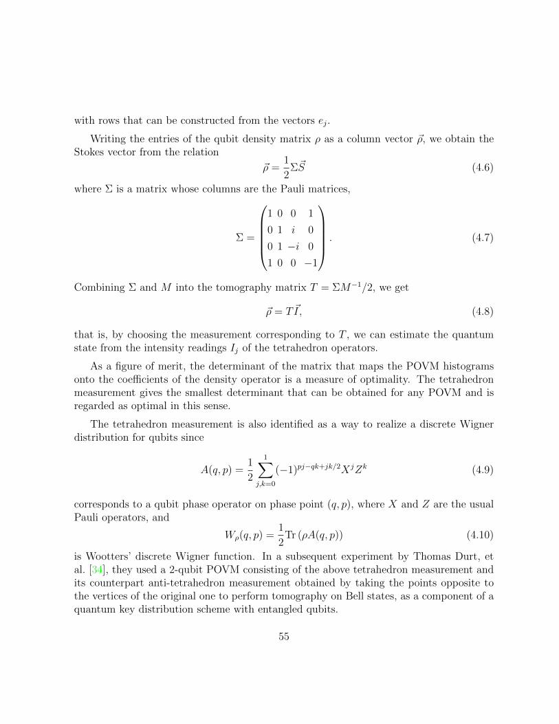
with rows that can be constructed from the vectors ej.

Writing the entries of the qubit density matrix ρ as a column vector ~ρ, we obtain theStokes vector from the relation

~ρ =1

2Σ~S (4.6)

where Σ is a matrix whose columns are the Pauli matrices,

Σ =

1 0 0 1

0 1 i 0

0 1 −i 0

1 0 0 −1

. (4.7)

Combining Σ and M into the tomography matrix T = ΣM−1/2, we get

~ρ = T ~I, (4.8)

that is, by choosing the measurement corresponding to T , we can estimate the quantumstate from the intensity readings Ij of the tetrahedron operators.

As a figure of merit, the determinant of the matrix that maps the POVM histogramsonto the coefficients of the density operator is a measure of optimality. The tetrahedronmeasurement gives the smallest determinant that can be obtained for any POVM and isregarded as optimal in this sense.

The tetrahedron measurement is also identified as a way to realize a discrete Wignerdistribution for qubits since

A(q, p) =1

2

1∑j,k=0

(−1)pj−qk+jk/2XjZk (4.9)

corresponds to a qubit phase operator on phase point (q, p), where X and Z are the usualPauli operators, and

Wρ(q, p) =1

2Tr (ρA(q, p)) (4.10)

is Wootters’ discrete Wigner function. In a subsequent experiment by Thomas Durt, etal. [34], they used a 2-qubit POVM consisting of the above tetrahedron measurement andits counterpart anti-tetrahedron measurement obtained by taking the points opposite tothe vertices of the original one to perform tomography on Bell states, as a component of aquantum key distribution scheme with entangled qubits.

55

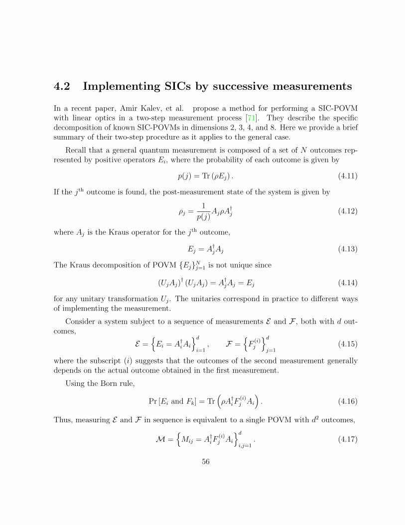
4.2 Implementing SICs by successive measurements

In a recent paper, Amir Kalev, et al. propose a method for performing a SIC-POVMwith linear optics in a two-step measurement process [71]. They describe the specificdecomposition of known SIC-POVMs in dimensions 2, 3, 4, and 8. Here we provide a briefsummary of their two-step procedure as it applies to the general case.

Recall that a general quantum measurement is composed of a set of N outcomes rep-resented by positive operators Ei, where the probability of each outcome is given by

p(j) = Tr (ρEj) . (4.11)

If the jth outcome is found, the post-measurement state of the system is given by

ρj =1

p(j)AjρA

†j (4.12)

where Aj is the Kraus operator for the jth outcome,

Ej = A†jAj (4.13)

The Kraus decomposition of POVM {Ej}Nj=1 is not unique since

(UjAj)† (UjAj) = A†jAj = Ej (4.14)

for any unitary transformation Uj. The unitaries correspond in practice to different waysof implementing the measurement.

Consider a system subject to a sequence of measurements E and F , both with d out-comes,

E ={Ei = A†iAi

}di=1

, F ={F

(i)j

}dj=1

(4.15)

where the subscript (i) suggests that the outcomes of the second measurement generallydepends on the actual outcome obtained in the first measurement.

Using the Born rule,

Pr [Ei and Fk] = Tr(ρA†iF

(i)j Ai

). (4.16)

Thus, measuring E and F in sequence is equivalent to a single POVM with d2 outcomes,

M ={Mij = A†iF

(i)j Ai

}di,j=1

. (4.17)

56

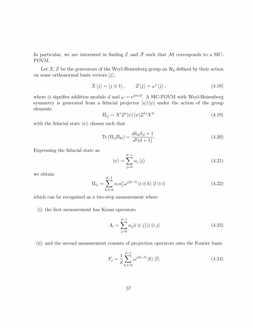
In particular, we are interested in finding E and F such that M corresponds to a SIC-POVM.

Let X,Z be the generators of the Weyl-Heisenberg group on Hd defined by their actionon some orthonormal basis vectors |j〉,

X |j〉 = |j ⊕ 1〉 , Z |j〉 = ωj |j〉 , (4.18)

where ⊕ signifies addition modulo d and ω = e2πi/d. A SIC-POVM with Weyl-Heisenbergsymmetry is generated from a fiducial projector |ψ〉〈ψ| under the action of the groupelements

Πij = X iZj|ψ〉〈ψ|Z†jX†i (4.19)

with the fiducial state |ψ〉 chosen such that

Tr (ΠijΠkl) =dδikδjl + 1

d2(d+ 1). (4.20)

Expressing the fiducial state as

|ψ〉 =d−1∑j=0

αj |j〉 (4.21)

we obtain

Πij =d−1∑k,l=0

αiα∗jω

j(k−l) |i⊕ k〉 〈l ⊕ i| (4.22)

which can be recognized as a two-step measurement where

(i) the first measurement has Kraus operators

Ai =d−1∑j=0

αj|i⊕ j〉〈i⊕ j| (4.23)

(ii) and the second measurement consists of projection operators onto the Fourier basis

Fj =1

d

d−1∑k,l=0

ωj(k−l) |k〉 〈l|. (4.24)

57

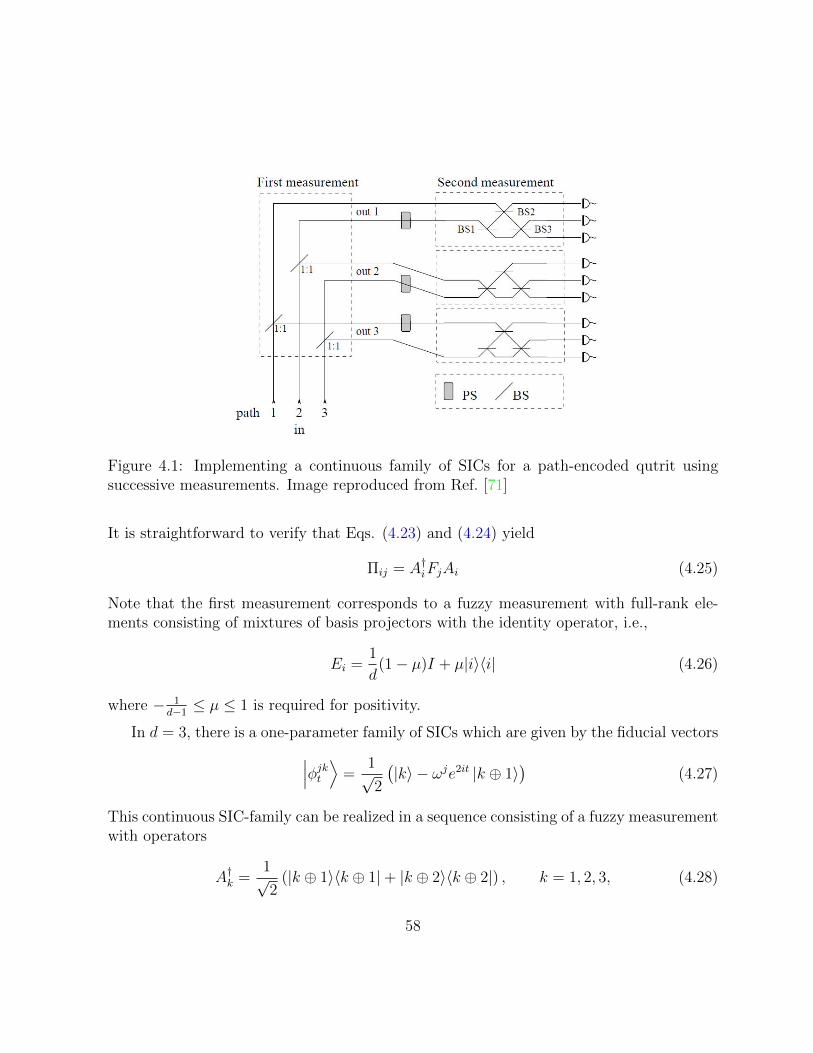
Figure 4.1: Implementing a continuous family of SICs for a path-encoded qutrit usingsuccessive measurements. Image reproduced from Ref. [71]

It is straightforward to verify that Eqs. (4.23) and (4.24) yield

Πij = A†iFjAi (4.25)

Note that the first measurement corresponds to a fuzzy measurement with full-rank ele-ments consisting of mixtures of basis projectors with the identity operator, i.e.,

Ei =1

d(1− µ)I + µ|i〉〈i| (4.26)

where − 1d−1≤ µ ≤ 1 is required for positivity.

In d = 3, there is a one-parameter family of SICs which are given by the fiducial vectors∣∣∣φjkt ⟩ =1√2

(|k〉 − ωje2it |k ⊕ 1〉

)(4.27)

This continuous SIC-family can be realized in a sequence consisting of a fuzzy measurementwith operators

A†k =1√2

(|k ⊕ 1〉〈k ⊕ 1|+ |k ⊕ 2〉〈k ⊕ 2|) , k = 1, 2, 3, (4.28)

58

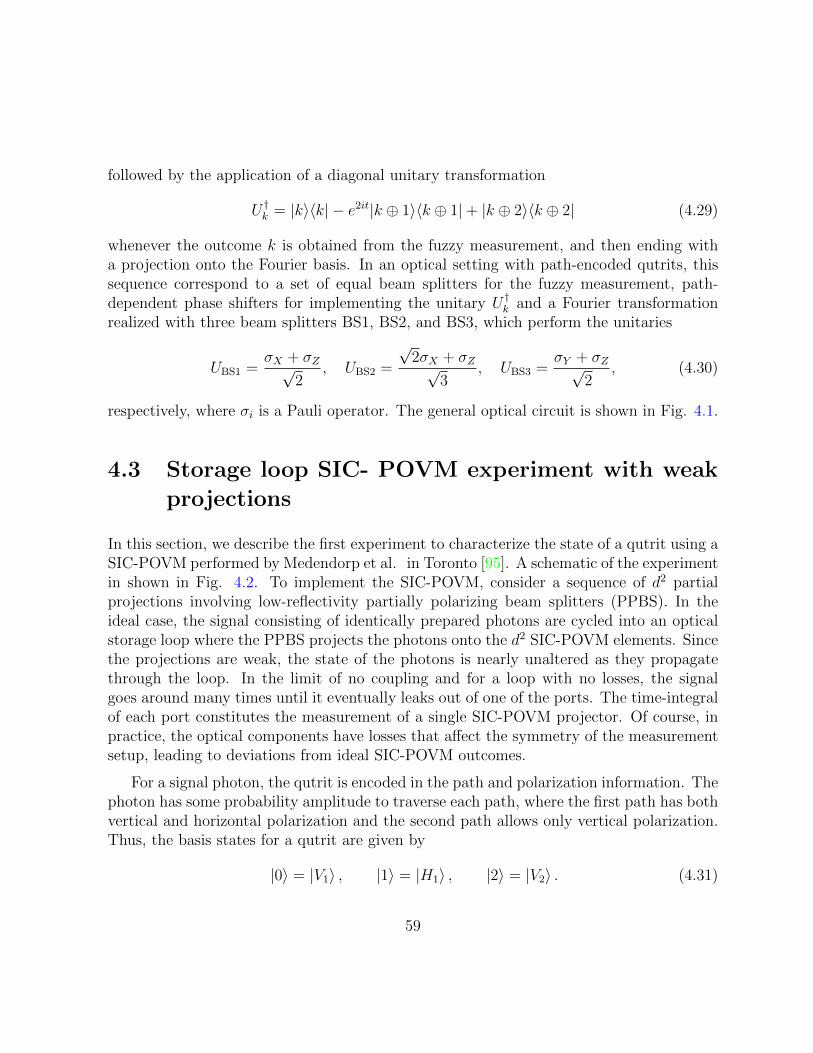
followed by the application of a diagonal unitary transformation

U †k = |k〉〈k| − e2it|k ⊕ 1〉〈k ⊕ 1|+ |k ⊕ 2〉〈k ⊕ 2| (4.29)

whenever the outcome k is obtained from the fuzzy measurement, and then ending witha projection onto the Fourier basis. In an optical setting with path-encoded qutrits, thissequence correspond to a set of equal beam splitters for the fuzzy measurement, path-dependent phase shifters for implementing the unitary U †k and a Fourier transformationrealized with three beam splitters BS1, BS2, and BS3, which perform the unitaries

UBS1 =σX + σZ√

2, UBS2 =

√2σX + σZ√

3, UBS3 =

σY + σZ√2

, (4.30)

respectively, where σi is a Pauli operator. The general optical circuit is shown in Fig. 4.1.

4.3 Storage loop SIC- POVM experiment with weak

projections

In this section, we describe the first experiment to characterize the state of a qutrit using aSIC-POVM performed by Medendorp et al. in Toronto [95]. A schematic of the experimentin shown in Fig. 4.2. To implement the SIC-POVM, consider a sequence of d2 partialprojections involving low-reflectivity partially polarizing beam splitters (PPBS). In theideal case, the signal consisting of identically prepared photons are cycled into an opticalstorage loop where the PPBS projects the photons onto the d2 SIC-POVM elements. Sincethe projections are weak, the state of the photons is nearly unaltered as they propagatethrough the loop. In the limit of no coupling and for a loop with no losses, the signalgoes around many times until it eventually leaks out of one of the ports. The time-integralof each port constitutes the measurement of a single SIC-POVM projector. Of course, inpractice, the optical components have losses that affect the symmetry of the measurementsetup, leading to deviations from ideal SIC-POVM outcomes.

For a signal photon, the qutrit is encoded in the path and polarization information. Thephoton has some probability amplitude to traverse each path, where the first path has bothvertical and horizontal polarization and the second path allows only vertical polarization.Thus, the basis states for a qutrit are given by

|0〉 = |V1〉 , |1〉 = |H1〉 , |2〉 = |V2〉 . (4.31)

59

Figure 4.2: SIC-POVM storage loop scheme implemented by partial projections over threeround trips. The PPBS labels indicate how the detector click is interpreted.

Figure 4.3: (a) Qutrit state encoding. (b) Implementing the X and Z gates.

The qutrit state encoding is shown in Fig. 4.3(a).

In the actual experiment, the SIC-POVM chosen was the one associated with thefiducial vector

|ψ〉 =1√2

(|0〉+ |1〉), (4.32)

which is the one of the exceptional SICs for t = π6. Part of the reason for choosing this SIC

is that it leads to SIC vectors which can be measured by projection onto the first path,since the zero component can always be put in the second path.

A schematic of the experimental apparatus is displayed in Fig. 4.4. The SIC-POVMmeasurement is obtained from partial projections and permuting through the SIC elementswith X and Z gates. The storage loop is constructed with 3 Z gates and 1 X gatewhich couple with the signal in 3 round trips. If n is the round trip number, the weak

60

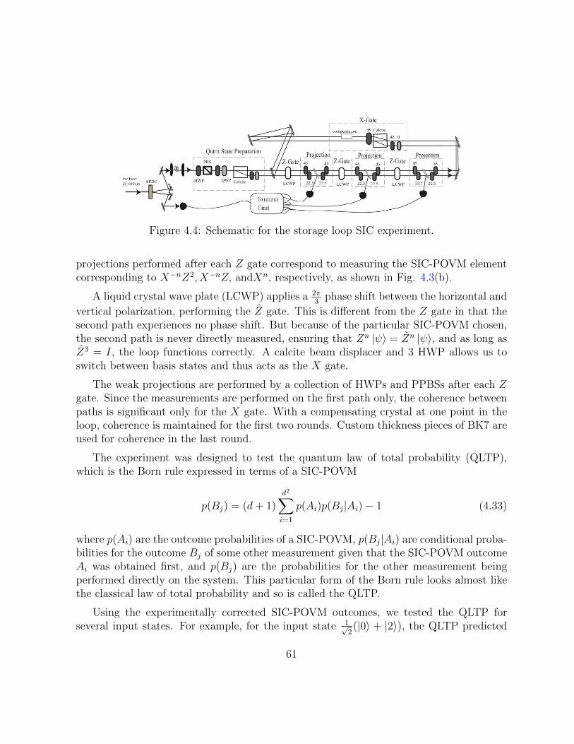
Figure 4.4: Schematic for the storage loop SIC experiment.

projections performed after each Z gate correspond to measuring the SIC-POVM elementcorresponding to X−nZ2, X−nZ, andXn, respectively, as shown in Fig. 4.3(b).

A liquid crystal wave plate (LCWP) applies a 2π3

phase shift between the horizontal and

vertical polarization, performing the Z gate. This is different from the Z gate in that thesecond path experiences no phase shift. But because of the particular SIC-POVM chosen,the second path is never directly measured, ensuring that Zn |ψ〉 = Zn |ψ〉, and as long asZ3 = I, the loop functions correctly. A calcite beam displacer and 3 HWP allows us toswitch between basis states and thus acts as the X gate.

The weak projections are performed by a collection of HWPs and PPBSs after each Zgate. Since the measurements are performed on the first path only, the coherence betweenpaths is significant only for the X gate. With a compensating crystal at one point in theloop, coherence is maintained for the first two rounds. Custom thickness pieces of BK7 areused for coherence in the last round.

The experiment was designed to test the quantum law of total probability (QLTP),which is the Born rule expressed in terms of a SIC-POVM

p(Bj) = (d+ 1)d2∑i=1

p(Ai)p(Bj|Ai)− 1 (4.33)

where p(Ai) are the outcome probabilities of a SIC-POVM, p(Bj|Ai) are conditional proba-bilities for the outcome Bj of some other measurement given that the SIC-POVM outcomeAi was obtained first, and p(Bj) are the probabilities for the other measurement beingperformed directly on the system. This particular form of the Born rule looks almost likethe classical law of total probability and so is called the QLTP.

Using the experimentally corrected SIC-POVM outcomes, we tested the QLTP forseveral input states. For example, for the input state 1√

2(|0〉 + |2〉), the QLTP predicted

61

the probability of measuring 1√2(|0〉 + i|2〉) to be 0.526 ± 0.009(stat) ± 0.03(sys), while

in a direct measurement we found 0.506 ± 0.004 ± 0.002. For the input state |0〉, theQLTP prediction for the probability of measuring 1√

2(|1〉+ |2〉) was 0.01 ± 0.0002(stat) ±

0.009(sys), while in a direct measurement we found 0.005 ± 0.0004 ± 0.001. These resultsare consistent with the QLTP.

4.4 Multiport scheme from Naimark dilation of SIC-

POVMs

In this section, we describe an experimental scheme for performing SIC-POVMs with in-tegrated optics. An integrated optical circuit is a device that combines multiple functionsfor manipulating photons analogous to a microchip for electronic systems, the essentialdifference being that the former works in optical wavelengths. Photonic integrated circuitsallows for compact, efficient, and scalable performance, which is important for optical sys-tems used to implement a quantum computation. Physical realizations of integrated opticsinclude silica-based planar lightwave circuit interferometers fabricated on a semiconductorchip [73,74,94,107], periodically poled lithium niobate waveguides in standard fiber opticstechnology [19,93,109,116] and the direct-write femtosecond laser technique for manufac-turing optical waveguides in dielectric materials [32, 92, 102], which allows one to realizethree-dimensional photonic circuits, in contrast with the flat architecture of conventionallithography.

The flexibility afforded by integrated optics makes it the natural candidate for realizingsomething called a multiport device, which is a blackbox for performing any discrete unitaryoperation through a sequence of qubit operations acting on various optical modes, in thecase of photonic systems [112]. An optical version of a multiport devices features a sequenceof beam splitters and phase shifters with parameters that can be adjusted to perform anyquantum gate operation, i.e., unitary transformation. Note that a qubit unitary acting onoptical modes transforms two input modes (k, l) into two output modes (k′, l′) accordingto (

k′

l′

)=

(eiφ sin θ eiφ cos θ

cos θ − sin θ

)(k

l

)(4.34)

and allows measurements to be done in any other basis. With a multiport device, unitaryoperations, and therefore arbitrary projective measurements, can also be realized in higher-dimensional quantum systems, providing a means of performing full state tomography witha quantum circuit, in particular, a means for realizing a SIC-POVM.

62

But how does one realize a measurement in terms of a unitary operation? Here itis important to recall a particular result called Naimark’s theorem [83]. In most commonversion of the theorem states that there is no loss in generality in considering only projectivemeasurements because any general measurement or POVM on a quantum system can beachieved by a joint projective measurement on the system and an ancilla, provided theancilla has large enough a dimension and that it is initialized to a known pure quantumstate [106].

In the finite dimensional case, there is a simple procedure for determining the projectivemeasurement that corresponds to a POVM. Suppose we have a POVM {Ei : i = 1, 2, ..., N}and each POVM operator Ei is proportional to a rank-1 projection, which is described bythe subspace spanned by ei ∈ HM . Given N > M and the POVM elements are notmutually orthogonal, we can construct the M ×N matrix

V = (e1 . . . eN) (4.35)

and look for an (N −M)×N matrix W such that

U =

(V

W

)(4.36)

is an N ×N unitary matrix. In this case, the projectors associated with the columns of Ucorrespond to the desired projective measurement. It is by using the Naimark extensionof SIC-POVMs that we can design experiments for realizing SIC-POVMs with opticalmultiport devices.

The method here is completely general in that the Naimark extension can be found forSIC-POVMs of any dimension but for concreteness, we describe experiments for qubit andqutrit SIC-POVMs [124]. Experiments that feature higher-dimensional quantum systemsare far from trivial, making the qutrit case more interesting but the qubit case is useful forillustrating the basic idea behind the experimental scheme with multiport devices and sowe consider it first.

4.4.1 Multiport Qubit SIC-POVM

Any qubit SIC-POVM is associated with the vertices of a regular tetrahedron circumscribedby the Bloch sphere. There are infinitely many ways to choose this tetrahedron but wemay choose the projectors corresponding to the set of vectors{(

1

0

),

1√3

(1√

2

),

1√3

(eiπ3

e−iπ3

√2

),

1√3

(e−i

π3

eiπ3

√2

)}. (4.37)

63

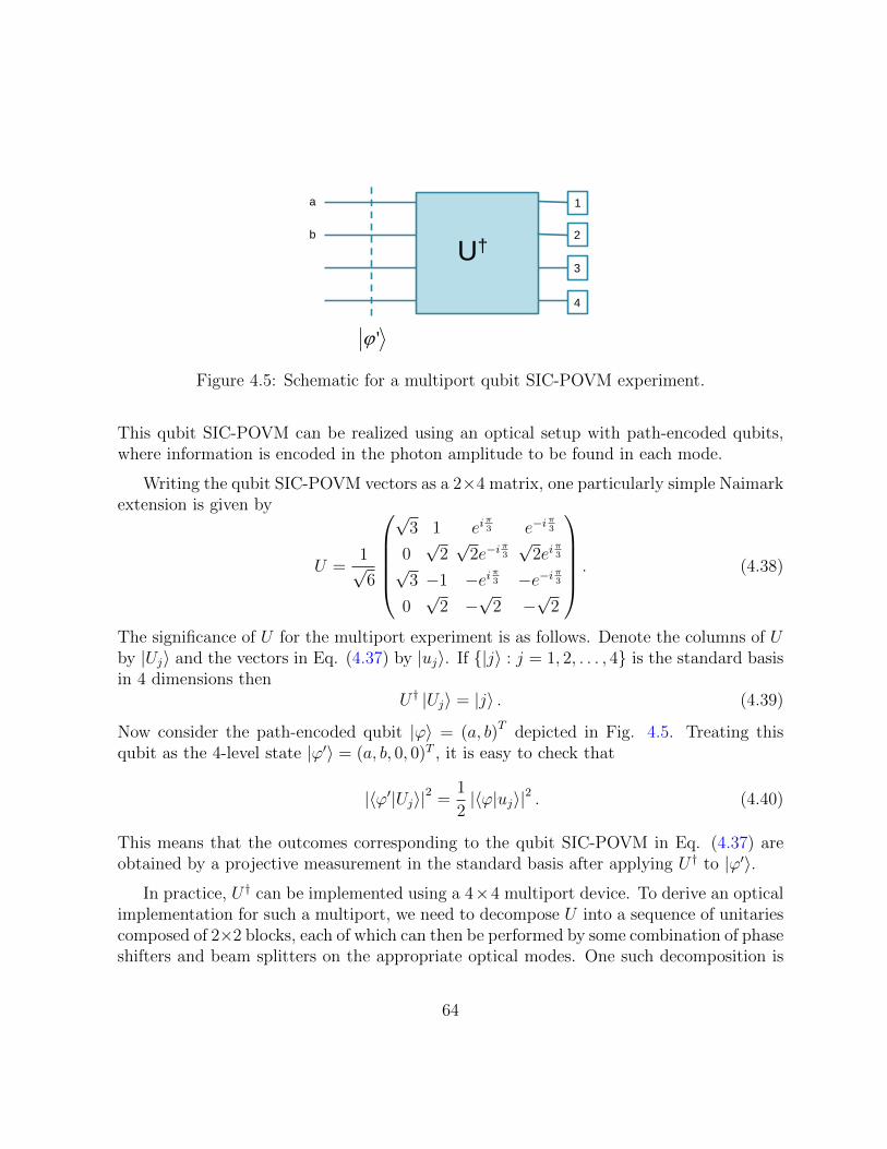
1

2

3

4

a

b

U†

'ϕ

Figure 4.5: Schematic for a multiport qubit SIC-POVM experiment.

This qubit SIC-POVM can be realized using an optical setup with path-encoded qubits,where information is encoded in the photon amplitude to be found in each mode.

Writing the qubit SIC-POVM vectors as a 2×4 matrix, one particularly simple Naimarkextension is given by

U =1√6

√

3 1 eiπ3 e−i

π3

0√

2√

2e−iπ3

√2ei

π3

√3 −1 −eiπ3 −e−iπ3

0√

2 −√

2 −√

2

. (4.38)

The significance of U for the multiport experiment is as follows. Denote the columns of Uby |Uj〉 and the vectors in Eq. (4.37) by |uj〉. If {|j〉 : j = 1, 2, . . . , 4} is the standard basisin 4 dimensions then

U † |Uj〉 = |j〉 . (4.39)

Now consider the path-encoded qubit |ϕ〉 = (a, b)T depicted in Fig. 4.5. Treating thisqubit as the 4-level state |ϕ′〉 = (a, b, 0, 0)T , it is easy to check that

|〈ϕ′|Uj〉|2 =1

2|〈ϕ|uj〉|2 . (4.40)

This means that the outcomes corresponding to the qubit SIC-POVM in Eq. (4.37) areobtained by a projective measurement in the standard basis after applying U † to |ϕ′〉.

In practice, U † can be implemented using a 4×4 multiport device. To derive an opticalimplementation for such a multiport, we need to decompose U into a sequence of unitariescomposed of 2×2 blocks, each of which can then be performed by some combination of phaseshifters and beam splitters on the appropriate optical modes. One such decomposition is

64

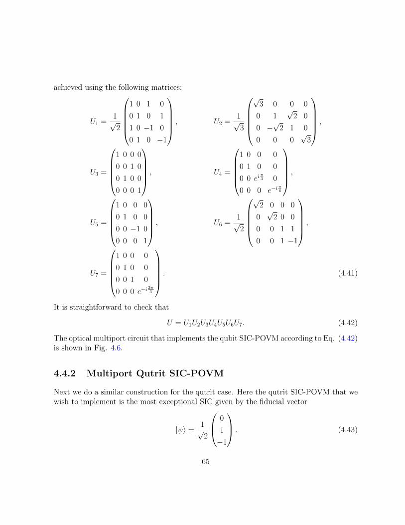
achieved using the following matrices:

U1 =1√2

1 0 1 0

0 1 0 1

1 0 −1 0

0 1 0 −1

, U2 =1√3

√

3 0 0 0

0 1√

2 0

0 −√

2 1 0

0 0 0√

3

,

U3 =

1 0 0 0

0 0 1 0

0 1 0 0

0 0 0 1

, U4 =

1 0 0 0

0 1 0 0

0 0 eiπ3 0

0 0 0 e−iπ6

,

U5 =

1 0 0 0

0 1 0 0

0 0 −1 0

0 0 0 1

, U6 =1√2

√

2 0 0 0

0√

2 0 0

0 0 1 1

0 0 1 −1

,

U7 =

1 0 0 0

0 1 0 0

0 0 1 0

0 0 0 e−i2π3

. (4.41)

It is straightforward to check that

U = U1U2U3U4U5U6U7. (4.42)

The optical multiport circuit that implements the qubit SIC-POVM according to Eq. (4.42)is shown in Fig. 4.6.

4.4.2 Multiport Qutrit SIC-POVM

Next we do a similar construction for the qutrit case. Here the qutrit SIC-POVM that wewish to implement is the most exceptional SIC given by the fiducial vector

|ψ〉 =1√2

0

1

−1

. (4.43)

65

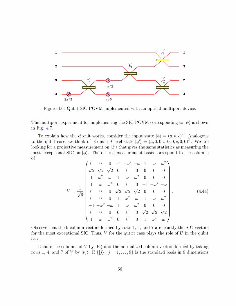
21

31

21

21 1

3

2

4 3/2π 6/π

3/π−

1

3

2

4

Figure 4.6: Qubit SIC-POVM implemented with an optical multiport device.

The multiport experiment for implementing the SIC-POVM corresponding to |ψ〉 is shownin Fig. 4.7.

To explain how the circuit works, consider the input state |φ〉 = (a, b, c)T . Analogousto the qubit case, we think of |φ〉 as a 9-level state |φ′〉 = (a, 0, 0, b, 0, 0, c, 0, 0)T . We arelooking for a projective measurement on |φ′〉 that gives the same statistics as measuring themost exceptional SIC on |φ〉. The desired measurement basis correspond to the columnsof

V =1√6

0 0 0 −1 −ω2 −ω 1 ω ω2

√2√

2√

2 0 0 0 0 0 0

1 ω2 ω 1 ω ω2 0 0 0

1 ω ω2 0 0 0 −1 −ω2 −ω0 0 0

√2√

2√

2 0 0 0

0 0 0 1 ω2 ω 1 ω ω2

−1 −ω2 −ω 1 ω ω2 0 0 0

0 0 0 0 0 0√

2√

2√

2

1 ω ω2 0 0 0 1 ω2 ω

. (4.44)

Observe that the 9 column vectors formed by rows 1, 4, and 7 are exactly the SIC vectorsfor the most exceptional SIC. Thus, V for the qutrit case plays the role of U in the qubitcase.

Denote the columns of V by |Vj〉 and the normalized column vectors formed by takingrows 1, 4, and 7 of V by |vj〉. If {|j〉 : j = 1, . . . , 9} is the standard basis in 9 dimensions

66

then V † |Vj〉 = |j〉. Moreover, one can check that

|〈φ′|Vj〉|2 =1

3|〈φ|vj〉|2 (4.45)

so the outcomes of the standard basis measurement after applying V † yield statistics thatis expected from the qutrit SIC-POVM.

The unitary V † can be realized with a 9× 9 multiport device. However, the particularstructure of V actually allows us to perform the SIC-POVM in terms of 3 × 3 unitaryoperations. The decomposition of V into a sequence of 3× 3 unitaries is possible becauseV exhibits the block-circulant structure

V =

A B C

C A B

B C A

(4.46)

where A,B,C are the 3×3 blocks in Eq. (4.44). V can be transformed into block diagonalform by

S = P ⊗ I3 ≡1√3

1 0 0 1 0 0 1 0 0

0 1 0 0 1 0 0 1 0

0 0 1 0 0 1 0 0 1

ω2 0 0 ω 0 0 1 0 0

0 ω2 0 0 ω 0 0 1 0

0 0 ω2 0 0 ω 0 0 1

ω 0 0 ω2 0 0 1 0 0

0 ω 0 0 ω2 0 0 1 0

0 0 ω 0 0 ω2 0 0 1

, P =

1√3

1 1 1

ω2 ω 1

ω ω2 1

. (4.47)

It is worth noting that the generalization of P to all higher dimensions is known as theBell multiport [85], and there is an efficient system for realizing the Fourier transform witha small number of optical elements [137].

Thus, we have

Q = SV S† ≡

Q1 0 0

0 Q2 0

0 0 Q3

(4.48)

67

where

Q1 =1√6

0 ω − ω2 ω2 − ω√

2√

2√

2

2 −1 −1

,

Q2 =1√6

ω2 − ω 0 ω − ω2

√2√

2√

2

−ω2 2ω2 −ω2

, (4.49)

Q3 =1√6

ω − ω2 ω2 − ω 0

√2

√2√

2

−ω −ω 2ω

.

Since S and Q are both composed of blocks of 3× 3 unitaries, this gives us the decom-position of V ,

V = S†QS, (4.50)

where Q has blocks acting on modes (1,2,3), (4,5,6), and (7,8,9) while S has blocks actingon modes (1,4,7), (2,5,8), and (3,6,9) of the input state |φ′〉. The qutrit SIC-POVMrequires V †, which translates into the scheme displayed in Fig. 4.7. Because each P † actson independent sets of modes, it is more economical in practice to include them in theinput state preparation, reducing the depth of the measurement circuit to just 2 parallellayers corresponding to the Qk and P . Since all components are 3 × 3 unitaries, a verycompact realization of the qutrit SIC-POVM is possible using integrated 3× 3 multimodeinterference devices.

To complete the construction, we determine optical networks for the unitaries P † andQ†k, k = 1, 2, 3. A circuit for Q†k can be constructed from the Euler decomposition of athree-dimensional rotation, permutation matrices, and diagonal unitaries. We can write

Q†k = GkRDk, (4.51)

where Dk are the diagonal matrices

D1 =

−i 0 0

0 1 0

0 0 1

, D2 =

−i 0 0

0 1 0

0 0 ω

, D3 =

−i 0 0

0 1 0

0 0 ω2

, (4.52)

68

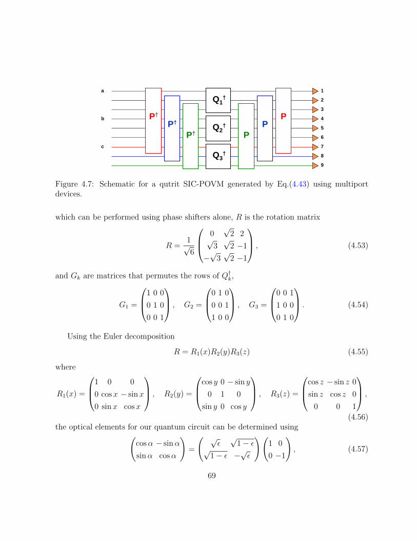
1

2

3

4

5

6

7

8

9

Q1†

Q2†

Q3†

P† P†

P† P P

P

a

b

c

Figure 4.7: Schematic for a qutrit SIC-POVM generated by Eq.(4.43) using multiportdevices.

which can be performed using phase shifters alone, R is the rotation matrix

R =1√6

0√

2 2√

3√

2 −1

−√

3√

2 −1

, (4.53)

and Gk are matrices that permutes the rows of Q†k,

G1 =

1 0 0

0 1 0

0 0 1

, G2 =

0 1 0

0 0 1

1 0 0

, G3 =

0 0 1

1 0 0

0 1 0

. (4.54)

Using the Euler decomposition

R = R1(x)R2(y)R3(z) (4.55)

where

R1(x) =

1 0 0

0 cos x − sinx

0 sinx cosx

, R2(y) =

cos y 0 − sin y

0 1 0

sin y 0 cos y

, R3(z) =

cos z − sin z 0

sin z cos z 0

0 0 1

,

(4.56)the optical elements for our quantum circuit can be determined using(

cosα − sinα

sinα cosα

)=

( √ε√

1− ε√

1− ε −√ε

)(1 0

0 −1

), (4.57)

69

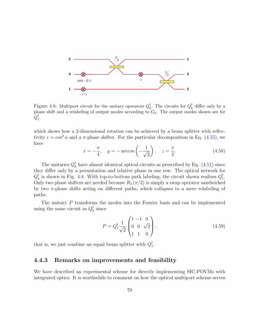
21

31

( ) 3/14 −kπ

2/π−

π

2

3

1

1

3

2

Figure 4.8: Multiport circuit for the unitary operators Q†k. The circuits for Q†k differ only by aphase shift and a relabeling of output modes according to Gk. The output modes shown are forQ†1.

which shows how a 2-dimensional rotation can be achieved by a beam splitter with reflec-tivity ε = cos2 α and a π-phase shifter. For the particular decomposition in Eq. (4.55), wehave

x = −π4, y = − arccos

(− 1√

3

), z =

π

2. (4.58)

The unitaries Q†k have almost identical optical circuits as prescribed by Eq. (4.51) sincethey differ only by a permutation and relative phase in one row. The optical network forQ†k is shown in Fig. 4.8. With top-to-bottom path labeling, the circuit shown realizes Q†1.Only two phase shifters are needed because R3 (π/2) is simply a swap operator sandwichedby two π-phase shifts acting on different paths, which collapses to a mere relabeling ofpaths.

The unitary P transforms the modes into the Fourier basis and can be implementedusing the same circuit as Q†k since

P = Q†11√2

1 −1 0

0 0√

2

1 1 0

, (4.59)

that is, we just combine an equal beam splitter with Q†1.

4.4.3 Remarks on improvements and feasibility

We have described an experimental scheme for directly implementing SIC-POVMs withintegrated optics. It is worthwhile to comment on how the optical multiport scheme serves

70

as an improvement over previous techniques and what possible issues there are regardingits practical feasibility.

A key component for realizing the scheme is the SIC-POVM decomposition into opticalnetworks. Designing the scheme for linear optics is practical given that various experimen-tal groups are already currently working on multimode interference experiments with pathencoded qudits but in principle the scheme can be realized with any setup that can performthe Naimark unitaries correspond to SIC-POVMs. As to the prescribed decomposition it-self, we would like to emphasize that our decomposition shows a remarkable improvementover the general procedure for discrete unitary operators as described by Reck, et al. [112].Reck’s method can be sketched in following way. Let d be the Hilbert space dimension andN = d2. Then any N -dimensional unitary operator can be realized by an optical circuitwith (N−1) beam splitters between modes 1 and 2, (N−2) beam splitters between modes2 and 3, and so on until one beam splitter between modes (N − 1) and N , a phase shifteraccompanying each beam splitter, and finally (N − 1) phase shifters before measuring theoutput. Counting all the optical elements needed, we obtain (N2 − 1) elements. Thus,by Reck’s method no more than (d4 − 1) elements are required to realize the unitary fora d-dimensional SIC-POVM, but for particular unitary operators, it is possible that con-siderably fewer elements are needed. For example, Reck’s method suggests that the 4× 4unitary for the qubit SIC-POVM needs 15 elements but our optical multiport scheme hereuses only 7 elements. Similarly, the unitary corresponding to a qutrit SIC-POVM wouldgenerally require 80 elements but the one we present here uses only 44 elements.

We also remark on how the optical multiport scheme for qutrit SIC-POVMs comparesto the storage loop experiment [95] of Sec 4.3. In that scheme, photons are sent into anoptical storage loop and the SIC-POVM is performed by weakly coupled PPBS, with a fullmeasurement completed after the signal makes 3 rounds. Because of the loop design, ituses only 22 elements for the measurement: 3 liquid crystal wave plates, 1 beam displacer,3 PPBS, and the rest are half wave plates. Ideally, each PPBS extracts an infinitesimalportion of the signal that circles the loop infinitely many times. In the actual experiment,each PPBS reflected about 3% of the horizontal polarization and 13% of the vertical po-larization. This led to a significant drop in visibilities even before we finish performingthe SIC-POVM. Even with compensation wave plates that help tune the visibility of in-terference between modes, the visibilities achieved were 74% and 36% for the first andsecond rounds, respectively. Errors due to beam deformation and other losses in the loopwere also corrected during the post-measurement analysis, but some of the results werestill off by as much as 20% from the theoretically expected values. An accurate assessmentof the sensitivity of the multiport scheme to losses in the optical elements will depend onthe actual apparatus used to realized it but because there is no weak coupling demand,

71

we expect it to be more robust to errors and show a vast improvement in performancecompared to the Medendorp results.

To properly assess the feasibility of the multiport experiment, it is important to knowhow sensitive the scheme is to fabrication errors or losses in the optical elements. Thespecifics will depend on the particular apparatus used for the multiport scheme. Forinstance, one might employ commercially available micro-optical chips used in some telecomdevices, which have built-in optical elements that can then be set to the appropriate values.Or in more standard cases, one is likely to fabricate the integrated optics circuit himself.In any case, the biggest issue will be maintaining the interferometric phase stability amongthe optical modes. For example, in the qutrit case, the fact that the Qk and P act ondifferent sets of modes means one has to actively check and correct for possibly unstablerelative phases, which is quite a nontrivial task at present. A way to possibly avoid thephase stability issue is to fabricate the 9×9 unitary for the qutrit case as a single nine-modeintegrated device, but since our decomposition involves 44 elements that might create itsown challenges.

72

Chapter 5

The SIC representation of quantumstates

Quantum foundations is the branch of physics that seeks to elucidate what the laws ofquantum mechanics imply about the nature of the physical phenomena it describes. Inparticular, it aims to identify a correct interpretation of the quantum formalism, whichwill hopefully provide a clear picture of reality in a quantum world.

So far we have studied properties of SICs mainly in the context of quantum information,where it is a special case of a generalized measurement appropriate for various tomographicpurposes. Here we shift gears and examine the role SICs play in understanding quantumtheory itself.

The conceptual significance of SICs follows from the fact that the set {Πi}d2

i=1 is linearlyindependent and thus forms a basis for the space of d-dimensional density operators. Thisallows us to define the bijective mapping ~p 7→ ρ,

ρ =d2∑i=1

[(d+ 1)p(i)− 1

d

]Πi, (5.1)

which establishes a one-to-one correspondence between probability distributions for a SICand quantum states represented by density operators. Therefore, the probabilities p(i)provide an equivalent description of quantum states, which is called the SIC representationand is the subject of this chapter.

73

5.1 Quantum states as degrees of belief

Progress in quantum foundations has generally meant taking the mathematical structureof quantum mechanics as given but establishing an account that identifies the real, physicalobjects implied by the theory, which is independent of any external observer. Numerousattempts to furnish such an account have led to a variety of interpretations that can bebroadly categorized into two camps, ontic and epistemic.

The ontic camp regards the quantum state as a real entity with an objective existenceakin to the physical properties possessed by a classical system. The standard approach isto identify mathematical symbols in the theory literally as some actual physical object. Itsuffices to consider 3 examples to understand how this works. One is the de Broglie-Bohmpilot wave theory, where particles exhibit quantum behavior by obeying essentially classicalequation but accompanied by a real wave function in configuration space that dictates thedynamics in a completely nonlocal fashion. Another is the class of spontaneous collapsetheories, of which the Ghirardi-Rimini-Weber (GRW) variant is most popular, which ac-cepts the usual unitary evolution of quantum systems but interrupts this occasionally withsome random nonlinear effect, removing the need for the process of measurement. Thelast one we mention is the many-worlds interpretation that introduces the idea of a mul-tiverse, obtained from a deterministic quantum state evolving into multiple branches withindependent realities, and where the probabilistic nature of quantum systems is merely anapparent effect of residing in a single branch of reality.

While the ontic approaches have their merits, the main issue with them is that they ap-pear mostly to be arbitrary quick fixes that are in no way made necessary by the quantumformalism. Moreover, to attribute reality to quantum states introduces a host of paradoxesthat one either accepts as necessary, like a wave function that connects everything nonlo-cally, or is explained away as being unobservable, like the unpredictable nonlinear collapsesor other branches of the multiverse.

The alternative is to adopt the epistemic view that quantum states are states of incom-plete knowledge about the system [61,122]. The epistemic approaches can be distinguishedby how they characterize the information encoded in quantum states. There are the ob-jectivists who ascribe this information to some hidden property of the quantum system,which is objective but not fully accessible. This lack of complete information leads to theprobabilities obtained from quantum states. On other hand, the subjectivists regard theinformation as representing an agent’s credible beliefs, reflecting his state of knowledgeabout the system.

Those who subscribe to a subjective view of quantum states are sometimes called

74

quantum Bayesians. The term “Bayesian” refers to the mathematician Thomas Bayes, whoprovided the first rigorous analysis of the problem of inference. To evaluate the probabilityof a hypothesis, a Bayesian starts with some prior probability, which is updated whennew information is available. This Bayesian notion of probability treats probabilities asan extension of logical reasoning and manipulates them according to a set of criteria fortesting consistency, in much the same way as logic tells us how to manipulate propositions.A probability assignment is a tool an agent uses to make decisions based on his beliefs. Therules of probability theory ensures that the agent accounts for those beliefs in a coherentway.

Rudolph Peierls [104] believed that the only legitimate way to understand quantummechanics is to consider the density operator as representing “our knowledge of the systemwe are trying to describe,” thereby advocating an epistemic view of quantum states. Asonce emphasized by Chris Fuchs and Asher Peres [44], “Quantum theory does not describephysical reality. What it does is provide an algorithm for computing probabilities for themacroscopic events that are the consequence of our experimental interventions.”

Chris Fuchs and Rudiger Schack push the Bayesian viewpoint further by stating thatthe information embodied by a quantum state represents an agent’s degrees of belief aboutthe future behavior of a quantum system. To distinguish their approach from other versionsof quantum Bayesianism, they have dubbed it as QBism. The general idea of a Bayesianapproach to quantum probabilities can actually be traced back to Lane Hughston in 1984,although he mentioned this in the context of introducing a nonlinear modification to theSchrodinger equation. By contrast, QBism does not make any radical changes to the quan-tum formalism. What QBism proposes is a personalist interpretation to the probabilitiesthat appear in quantum theory. The personalist Bayesian considers probability theory asa calculus of consistency about one’s beliefs, irrespective of the source of those beliefs.Hence, a probability is a mere calculational tool for a consistent accounting of information;it does not exist as an objective property of the system.

One important implication of subjective quantum probabilities is that there is no suchthing as a correct quantum state for a system, since everyone assigns a state according tohis own beliefs. There are circumstances, however, where two agents are logically led to thesame state. For instance, when we speak of determining an unknown quantum state from atomographic measurement, the de Finetti theorem says that what we really do is update aprior probability assignment assuming the systems being measured are exchangeable [26].As long as an agent does not assign a zero probability to some state, the theorem shows thatindependent observers with minimal agreement in beliefs will converge to some productstate assignment for the exchangeable systems.

75

But if the proper way of thinking about quantum states just a matter of interpretingprobabilities correctly, why is the quantum formalism not directly written in the languageof probabilities, instead of using concepts in Hilbert space? Actually, it is always possible toformulate quantum theory in terms of probabilities. We only need the sort of measurementthat can be used to determine a quantum state uniquely in a tomography experiment.For QBism, this key ingredient is a SIC-POVM, which establishes a one-to-one mappingbetween density operators and probabilities via Eq. (5.1).

In quantum theory, probabilities are computed from the Born rule. This means thatwe can also think of these probabilities as subject to the agent who assigns them. The onlydifference in the quantum case is that in order to be consistent with the rules of quantummechanics, the probability assignment must also be constrained by the Born rule, whichwhen written in terms of a SIC measurement {Πi}d

2

i=1 gives

q(j) = (d+ 1)d2∑i=1

p(i)p(j|i)− 1, (5.2)

where p(i) is the probability of outcome πi measured directly, q(j) is the probability ofoutcome Ej of any other measurement {Ej}Nj=1 measured directly, and p(j|i) = Tr (ΠiEj)is the conditional probability of Ej given Πi. Because of its similarity to the classical law oftotal probability, Eq. (5.2) is also called the quantum law of total probability. Fuchs andSchack develop an axiomatic framework for reconstructing quantum theory by treatingEq. (5.2) as an empirical addition to Bayesian probability theory [47]. In the next twochapters, we explore the structure of quantum states in the QBist framework.

5.2 Representing quantum states with SICs

Our first task is to find the conditions for a SIC probability distribution to be a pure state.Recall that a density operator ρ corresponds to a pure quantum state if and only if it is arank-1 projector, i.e., ρ2 = ρ. The SIC representation for ρ is given by Eq. (5.1). As long as~p is a probability distribution, ρ in Eq. (5.1) is guaranteed to be a Hermitian operator. Inthis case, a remarkable theorem independently shown by Nick Jones and Noah Linden [70],and by Steve Flammia [41] states that an equivalent condition for pure states is given by

Tr(ρ2)

= Tr(ρ3)

= 1. (5.3)

76

Translating Eq. (5.3) in terms of SICs, we obtain constraints on SIC probabilities associatedwith pure states. From Tr (ρ2) = 1 we obtain∑

i

p(i)2 =2

d(d+ 1). (5.4)

From Tr (ρ3) = 1, we can work out that∑i,j,k

Tijkp(i)p(j)p(k) =d+ 7

(d+ 1)3(5.5)

whereTijk = Tr (ΠiΠjΠk) (5.6)

are the triple products we first encountered in Chapter 3.

Geometrically, we can think of the SIC probabilities as points on a simplex embeddedin real vector space. Then Eq. (5.4) says that the probabilities corresponding to pure stateslie on a sphere while Eq. (5.5) picks out a manifold of points on that sphere that actuallycorresponds to quantum states. Since quantum state space is a compact, convex set, theconvex hull of probabilities satisfying Eq. (5.4) and Eq. (5.5) corresponds to the set of allquantum states. Moreover, because the extreme points lie on a sphere, it means the lengthof any vector belonging to the set is less than or equal to the radius of the sphere. Thisimplies that the scalar product of two probability distributions is bounded. The upperbound is given by

~p · ~q ≤ 2

d(d+ 1), (5.7)

which follows from the radius of the sphere, while a lower bound can be obtained fromconsidering Tr (ρσ) ≥ 0 for density operators, which translates into

d(d+ 1)~p · ~q − 1 ≥ 0 =⇒ ~p · ~q ≥ 1

d(d+ 1). (5.8)

An important observation that we will exploit throughout the rest of our discussion isthe fact that the real part of Tijk is sufficient in Eq. (5.5) since∑i,j,k

Tijkp(i)p(j)p(k) =1

2

∑i,j,k

Tr (ΠkΠjΠi) p(k)p(j)p(i) +1

2

∑i,j,k

Tr (ΠiΠjΠk) p(i)p(j)p(k)

=∑i,j,k

1

2

[Tr(

(ΠiΠjΠk)†)

+ Tr (ΠiΠjΠk)]p(i)p(j)p(k),

=∑i,j,k

Tijkp(i)p(j)p(k) (5.9)

77

where Tijk = Re [Tijk]. This also follows from the fact that the imaginary parts of Tijk arecompletely antisymmetric.

For Tr (ρ3) = 1, we get another expression in terms of the structure coefficients Sijk byusing ∑

k

Sijk =dδij + 1

d+ 1, (5.10)

which is obtained by taking the trace of

ΠiΠj =d2∑k=1

SijkΠk. (5.11)

Performing the algebra, we get∑i,j,k

Sijkp(i)p(j)p(k) =4

d(d+ 1)2(5.12)

where we may also replace Sijk with just the real parts Sijk.

Actually, we can get a condition for pure state probabilities directly from the idempo-tence condition ρ = ρ2 if we plug in ρ from Eq. (5.1) and take the trace of both sides,yielding

p(k) =(d+ 1)2

3d

∑i,j

Tijkp(i)p(j)−1

3d(5.13)

for k = 1, 2, ..., d2. The same condition but with structure coefficients is given by

p(k) =(d+ 1)

3

∑i,j

Sijkp(i)p(j) +2

3d(d+ 1). (5.14)

Because we will always be concerned with probability distributions obtained from SICs,any probability distribution that satisfies Eq. (5.4) and Eq. (5.5) or Eq. (5.12) will also becalled a pure state, which is implicitly identified with a rank-1 projector via Eq. (5.1).

We obtain a slight simplification if we note that

Tiii = 1, Tijj = Tjij = Tjji =1

d+ 1, (5.15)

from which it follows that

Siii = 1, Sijj = Sjij =1

d+ 1, Sjji = 0. (5.16)

78

Substituting these values into Eq.(5.12) gives∑i

p(i)3 + 2

(1

d+ 1

∑i

∑j 6=i

p(i)2p(j)

)+∑i 6=j 6=k

Sijkp(i)p(j)p(k) (5.17)

where using Eq.(5.4) and arranging terms, we get

d− 1

d+ 1

∑i

p(i)3 +∑i 6=j 6=k

Sijkp(i)p(j)p(k) = 0, (5.18)

5.3 Pure states as fixed points of a map

If we look at Eq. (5.18), we see that the left-hand side can be regarded of as a real-valuedscalar function

F (~p) =

(d− 1

d+ 1

)∑i

p(i)3 +∑i 6=j 6=k

Sijkp(i)p(j)p(k) (5.19)

acting on probability vectors. In this case, we get the condition that for ~p satisfying

~p · ~p =2

d(d+ 1), (5.20)

then F (~p) = 0 for pure states. So in the SIC representation, the intricate geometry of theconvex set of quantum states that is a consequence of the positivity conditions on densityoperators appears to be encoded primarily in this cubic constraint. Thus, it is useful toknow some of the properties of F (~p).

One of our attempts to find a some simple property of F (~p) was to take derivativesof it with respect to the probabilities p(i). This led us to an alternative way to definepure states in terms of the fixed points of a certain mapping from the simplex to the realvector space in which the simplex is embedded. Fixed points are interesting because inmany different contexts, they are related to the concepts of stability and equilibrium. Forinstance, in areas of study where the function describes an iterative process, the importantfixed points describe values for which the function tends to converge, in which case thefixed points are said to be attractive.

To construct the fixed point mapping for pure states, we start by computing the gradientof F (~p), which is obtained from taking its partial derivatives with respect to p(k):

∂F (~p)

∂p(k)= 3

(d− 1

d+ 1

)p(k)2 + 3

∑i 6=j( 6=k)

Sijkp(i)p(j) (5.21)

79

where the factor of 3 in the second term on the right-hand side is because

Sijk = Sjki = Skij, for i 6= j 6= k, (5.22)

each of which should be counted separately. The notation ( 6= k) is meant to indicate thatthe indices i, j, k are all distinct but there is no sum over k.

We note that∑i,j

Sijkp(i)p(j) =∑j( 6=k)

Skjkp(k)p(j) +∑i 6=k

Sikkp(i)p(k)

+∑i(6=k)

Siikp(i)2 + p(k)2 +

∑i 6=j( 6=k)

Sijkp(i)p(j). (5.23)

Substituting the known values of Sijk in Eq. (5.16) into Eq. (5.23) we have∑i,j

Sijkp(i)p(j) =2

d+ 1p(k) +

(d− 1

d+ 1

)p(k)2 +

∑i 6=j 6=k

Sijkp(i)p(j), (5.24)

Plugging this into Eq. (5.13), we get

p(k) = (d+ 1)

∑i 6=j(6=k)

Sijkp(i)p(j) +

(d− 1

d+ 1

)p(k)2

+2

d(d+ 1). (5.25)

Comparing Eq. (5.21) with Eq. (5.25), we finally obtain

p(k) =(d+ 1)

3

∂F

∂p(k)+

2

d(d+ 1). (5.26)

We can summarize the main result as follows: consider the mapping

G : ∆d2 → Rd2 ; ~p 7→ ~q (5.27)

from probability distributions ~p ∈ ∆d2−1 to vectors ~q ∈ Rd2 such that

~q = G(~p) =(d+ 1)

3~∇F (~p) +

2

d(d+ 1)~J (5.28)

80

where ~∇F is the gradient of Eq. (5.19) and ~J is the vector of all ones,

~J =

1...

1

, (5.29)

that is, it is a column vector with all d2 entries equal to 1. The pure states are then givenby the fixed points of G,

G(~p) = ~p (5.30)

provided thatd2∑i=1

p(i)2 =2

d(d+ 1). (5.31)

5.4 Pure states as stationary points of a map

In constructing the fixed point mapping in Eq. (5.28), we used derivatives of F (~p). Oncewe have derivatives of a function, we can ask for the its stationary points, which can be aminimum, maximum, or a saddle point. Stationary points are important for smooth real-valued functions since minima and maxima tend to signify optimal values in many contexts.In this section, we show the probability vectors representing pure states correspond to thestationary points of a certain map, and maybe knowing whether they are minimum ormaximum points of this map will tell us something new about pure states.

The form of Eq. (5.28) suggests that one can find a function M(~p) such that ~∇M(~p) = ~0for SIC probabilities ~p representing pure states. To construct the function M , we use alemma by Kimura [78] that expresses the positivity condition for density operators in termsof trace powers of ρ. Define

a1 = Tr (ρ) ,

a2 =Tr (ρ)2 − Tr (ρ2)

2,

a3 =1

6

[Tr (ρ)3 − 3Tr (ρ) Tr

(ρ2)

+ 2Tr(ρ3)], (5.32)

where a0 = 1, a1, a2, and a3 are first few coefficients of the characteristic polynomial of ρ,

det(λI − ρ) =d∑i=0

aixd−i = 0. (5.33)

81

If a1 = 1 and a2 = a3 = 0, then

Tr (ρ) = Tr(ρ2)

= Tr(ρ3)

= 1, (5.34)

so ρ must be a pure state, according to Eq. (5.3).

To derive M , we will first relax some of the usual conditions on ρ. In particular, we donot assume that Tr (ρ) = 1. We will then show that

M(~p) =1

6

[Tr (ρ(~p))3 − 3Tr (ρ(~p)) Tr

(ρ(~p)2

)+ 2Tr

(ρ(~p)3

)], (5.35)

where ρ(~p) is the density operator expressed in the SIC representation given by Eq. (5.1).

Calculating the required traces:

Tr (ρ) = (d+ 1)∑i

p(i)− d, (5.36)

Tr(ρ2)

= d (d+ 1)∑i

p(i)2 + (d+ 1)

(∑i

p(i)

)2

− 2 (d+ 1)∑i

p(i) + d,

Tr(ρ3)

= d (d+ 1)2∑i 6=j 6=k

Sijkp(i)p(j)p(k)− d+ d (d+ 1) (d− 1)∑i

p(i)3

+ 3 (d+ 1)∑i

p(i) + 2d (d+ 1)∑i

p(i)2∑i

p(i)− 3d (d+ 1)∑i

p(i)2

− 3 (d+ 1)

(∑i

p(i)

)2

+ (d+ 1)

(∑i

p(i)

)3

+ d (d+ 1)∑i

p(i)2∑i

p(i).

The components of ~∇M are given by

∂M

∂p(k)=

1

6

[3Tr (ρ)2 ∂Tr (ρ)

∂p(k)− 3Tr (ρ)

∂Tr (ρ2)

∂p(k)− 3

∂Tr (ρ)

∂p(k)Tr(ρ2)

+ 2∂Tr (ρ3)

∂p(k)

]. (5.37)

82

Differentiating the trace powers in Eq. (5.36), we get

∂Tr (ρ)

∂p(k)= d+ 1,

∂Tr (ρ2)

∂p(k)= 2d (d+ 1) p(k) + 2 (d+ 1)

∑i

p(i)− 2 (d+ 1) , (5.38)

∂Tr (ρ3)

∂p(k)= 3d (d+ 1)2

∑i 6=j(6=k)

Sijkp(i)p(j) + 3d(d2 − 1

)p(k)2 + 2d (d+ 1)

∑i

p(i)2

+ 4d (d+ 1) p(k)∑i

p(i) + 3 (d+ 1)− 6d (d+ 1) p(k)− 6 (d+ 1)∑i

p(i)

+ 3 (d+ 1)

(∑i

p(i)

)2

+ 2d (d+ 1) p(k)∑i

p(i) + d (d+ 1)∑i

p(i)2.

Next we substitute Eq. (5.38) into Eq. (5.39) and demand that ~p be a probabilitydistribution. After some algebra, we arrive at

∂M(~p)

∂p(k)

∣∣∣∣∣∑i p(i)=1

=1

6

{6d(d+ 1)

[(d+ 1

3

)∂F

∂p(k)− p(k)

]

+[6d(d+ 1)− 3d(d+ 1)2

]∑i

p(i)2 + 6(d+ 1)

}. (5.39)

where we used Eq. (5.21) in the previous section. To show that Eq. (5.39) vanishes forpure states, we can rewrite it as

∂M(~p)

∂p(k)=

1

6

{6d(d+ 1)

[(d+ 1

3

)∂F

∂p(k)− p(k) +

∑i

p(i)2

](5.40)

+

[−3d(d+ 1)2

∑i

p(i)2 + 6(d+ 1)

]},

= d(d+ 1)

[(d+ 1

3

)∂F

∂p(k)− p(k) +

2

d(d+ 1)

]− d(d+ 1)2

2

[∑i

p(i)2 − 2

d(d+ 1)

]= 0.

where the first term is zero because it just Eq. (5.28) while the second term is zero if the

83

probability distribution obeys lies on the sphere containing pure states,

~p · ~p =2

d(d+ 1). (5.41)

We summarize the result here: consider the function M : Rd2 → R that maps realvectors ~p to real numbers M(~p),

M(~p) =1

6

[Tr (ρ)3 − 3Tr (ρ) Tr

(ρ2)

+ 2Tr(ρ3)], (5.42)

where

ρ =∑i

[(d+ 1)p(i)− 1

d

]Πi. (5.43)

If ~p corresponds to a probability distribution then ~p determines a pure quantum state ifand only if

M(~p) = 0 and ~∇M(~p) = ~0 (5.44)

provided that

~p · ~p =2

d(d+ 1). (5.45)

Therefore, a probability distribution ~p obeying Eq. (5.45) is a pure state if and only if itis a stationary point of M .

As you may already suspect, since the function M(~p) depends on ~p only through theSIC representation, it seems that its stationary points are pure states independent of therepresentation used for ρ. This is indeed the case. Consider

ρ(~a) =∑j

ajAj (5.46)

for some basis {Aj} for the space of density operators, or more generally, for the space ofHermitian operators. Supposing that Tr (ρ) = 1,

M(ρ) =1

6

[1− 3Tr

(ρ(~a)2

)+ 2Tr

(ρ(~a)3

)]. (5.47)

We then have

∂M(~a)

∂ak= −3

∂Tr (ρ2)

∂ak+ 2

∂Tr (ρ3)

∂ak= −6Tr

[(ρ− ρ2

) ∂ρ∂ak

](5.48)

84

Since∂ρ

∂ak= Ak 6= 0 (5.49)

then Eq. (5.48) is equal to zero for any k if and only if ρ = ρ2, that is, ρ is a rank-1

projector. Thus, M = 0 and ~∇M = 0 define pure states for any representation ρ(~a)assuming only that Tr (ρ) = 1.

The next logical question is, what sort of stationary points are pure states? Theconventional way to determine this is by computing the eigenvalues of the Hessian matrixH(M), which has elements

[H(M)]ij =∂2M(~p)

∂p(j)∂p(i)(5.50)

evaluated at the stationary points ~p. According to the second partial derivative test, ifthe eigenvalues of H(M) are all positive (negative) then the stationary point is a localminimum (maximum). If H(M) has a mix of positive and negative eigenvalues then ~p is asaddle point. If there are any zero eigenvalues then the test is deemed inconclusive.

For the Hessian matrix H(M), we need the second partial derivatives of the traces:

∂2Tr (ρ)

∂p(j)∂p(k)= 0,

∂2Tr (ρ2)

∂p(j)∂p(k)= 2d(d+ 1)δjk + 2(d+ 1)p(j), (5.51)

∂2Tr (ρ3)

∂p(j)∂p(k)= 6d(d+ 1)

[(d+ 1)

∑i

Sijkp(i) + p(j) + p(k)

]+ 6(d+ 1)

[∑i

p(i)− 1

]

+ 6d(d+ 1)δjk

[(d− 1)p(j) +

∑i

p(i)− 1

].

Then the elements of H(M) are given by

∂2M(~p)

∂p(j)∂p(k)=

1

6

[6Tr (ρ)

∂Tr (ρ)

∂p(j)

∂Tr (ρ)

∂p(k)+ 3Tr

(ρ2) ∂2Tr (ρ)

∂p(j)∂p(k)

− 3∂Tr (ρ)

∂p(j)

∂Tr (ρ2)

∂p(k)− 3Tr (ρ)

∂2Tr (ρ2)

∂p(j)∂p(k)

− 3∂2Tr (ρ)

∂p(j)∂p(k)Tr(ρ2)− 3

∂Tr (ρ)

∂p(k)

∂Tr (ρ2)

∂p(j)+ 2

∂2Tr (ρ3)

∂p(j)∂p(k)

],

85

which we would like to evaluate when ~p is a probability distribution.

Using a specific example, we consider the example of pure states generated by themost exceptional SIC in d = 3. We performed numerical calculations where we randomlygenerate a pure state ρ and solve for its corresponding SIC probability distribution ~p.Then, we computed the eigenvalues of the Hessian matrix H(M) and we found that for allqutrit pure states considered

eigenvalues of H(M) = {36,−12,−12,−12, 0, 0, 0, 0, 0}. (5.52)

Because it contains zero eigenvalues, according to the second partial derivative test formultivariable functions, this result is unfortunately inconclusive. However, in the caseof qutrits, we do know what are stationary points are because the function M(~p) justcorresponds to the determinant of the corresponding density operator, Det(ρ). Since thisis equal to the product of the eigenvalues, it is minimized by any boundary state, whichhas M(~p) = 0. But only the pure states will have vanishing first partial derivatives so theyare the minimum points among quantum states.

This observation also helps us explain the set of eigenvalues we obtained in Eq. (5.52).There are 5 zeroes because the manifold of pure states for qutrits is 5-dimensional, so inall likelihood, the zeroes correspond to directions that move towards other pure states. Wehave one positive eigenvalue so M(~p) increases parallel to the direction of that eigenvector.We have 3 negative eigenvalues which means M(~p) can become negative in these directions;however, moving in those directions probably takes you out of the subset of the probabilitysimplex associated with quantum states.

Something similar can be used to argue that the pure states are minimum points inhigher dimensions. Although M(~p) is no longer the determinant, nonetheless it correspondsto the sum of various combinations of the product of 3 eigenvalues of ρ. (Alternatively,it corresponds to one of the coefficients in Kimura’s lemma 5.8.1 in Sec.!5.8, which shouldbe non-negative for a density operator.) This means that it will always be bounded belowby zero, which is attained by any boundary state with at most 2 nonzero eigenvalues. Butthe results in this section tell us that only the pure states corresponds to stationary pointsso they are the minimum ones for probability vectors corresponding to quantum states.

5.5 Rotations relating different SIC representations

In any finite dimension, a pair of distinct SICs will yield two different sets of probabilityvectors corresponding to quantum states. In this section, we will show that the probabilityvectors obtained from any two distinct SICs are related by an orthogonal transformation.

86

Suppose we have a pair of distinct SICs with elements Π′i and Πj, respectively. Inthe vector space of operators, Π′i and Πj correspond to the vertices of 2 identical regularsimplices, which means there must exist a rotation between them. Formally, because a SICforms a basis in the space of operators, we can write

Π′i =∑k

RijΠj. (5.53)

Since every SIC element has unit trace, taking the trace on both sides of Eq. (5.53) givesus ∑

j

Rij = 1. (5.54)

Multiplying the left-hand side of Eq.(5.53) by Π′j and the right-hand side by∑

lRjlΠl, wehave

Tr(Π′iΠ

′j

)=∑k,l

RikRjlTr (ΠkΠl) ,

dδij + 1

d+ 1=∑k,l

RikRjl

(dδkl + 1

d+ 1

),

δij =∑k

RikRjk. (5.55)

which is just the orthogonality condition.

We can also use Eq. (5.53) to calculate triple products:

Tr(Π′iΠ

′jΠ′k

)= Tr

(∑x

RixΠx

∑y

RjyΠy

∑z

RkzΠ′z

). (5.56)

This tells us thatT ′ijk =

∑x,y,z

RixRjyRkzTx,y,z. (5.57)

Recall the cubic equation for pure states in Eq. (5.5). Suppose we are given two probabilitydistributions ~p′ and ~p representing the same quantum state but for two SICs with elements

87

Π′i and Πj, respectively. Using Eq. (5.57) we have

d+ 7

(d+ 1)3=∑i,j,k

T ′ijkp′(i)p′(j)p′(k),

=∑i,j,k

(∑x,y,z

RixRjyRkzTx,y,z

)p′(i)p′(j)p′(k),

=∑x,y,z

Tx,y,zp(x)p(y)p(z), (5.58)

which implies that

p′(i) =∑j

Rijp(j). (5.59)

Thus, the rotation between two probability vectors representing the same quantum statefor two distinct SICs is the same rotation that relates the SICs in Eq. (5.53). Because thepure states are the extreme points, by linearity, the same condition holds for their convexhull, that is, all other quantum states.

Eq. (5.55) tells us that the sum of every row of the matrix Rij is one, as it should beif R~p is to be a valid probability distribution. We also expect

∑iRij = 1 since R must

be unital, that is, it should preserve the uniform distribution, which corresponds to themaximally mixed state for any SIC.

Observe that Eq. (5.53) tells us exactly how to construct the orthogonal transformationbetween the probability spaces generated by distinct SICs: the expansion coefficients thatwe get when we express one SIC in terms of the other form the elements of the desiredorthogonal matrix. Furthermore, the resulting orthogonal matrix is such that it mapsbetween probability vectors representing the same quantum state. In Sec. 6.2, we willuse this to explicitly construct the rotation matrix between the probability vectors of twodistinct qutrit SICs.

5.6 Fidelity of quantum states

In quantum information, the fidelity of quantum states gives a measure for how similartwo quantum states can be. For a pair of pure states |ψ〉 and |φ〉, the fidelity F (|ψ〉 , |φ〉)is given by

F (|ψ〉 , |φ〉) = |〈φ|ψ〉|. (5.60)

88

In general, given density matrices ρ and σ,

F (ρ, σ) = Tr

(√√ρσ√ρ

)(5.61)

where M =√ρ is the unique square root matrix obtained from the spectral decomposition

of ρ such that M2 = ρ. This definition can be thought of as the quantum generalizationof the fidelity of two probability vectors ~p and ~q:

F (~p, ~q) =∑i

√p(i)q(i). (5.62)

Now consider two density operators ρ and σ expressed in terms of the same SIC {Πi}d2

i=1:

ρ =d2∑r=1

[(d+ 1)pr −

1

d

]Πr, σ =

d2∑s=1

[(d+ 1)qs −

1

d

]Πs. (5.63)

The commutator [ρ, σ] is given by

[ρ, σ] = (d+ 1)2∑r,s

prqs (ΠrΠs − ΠsΠr)

= (d+ 1)2∑r,s

prqs∑t

JrstΠt (5.64)

where Jrst are the structure constants of the Lie algebra gld(C) in the basis defined by theSIC that we saw in Sec. 3.7. So ρ and σ commute when∑

r,s,t

prqsJrstΠt = 0. (5.65)

Because a SIC is a linearly independent set, this implies that for all t,∑r,s

prJrstqs = ~p · Jt~q = 0, (5.66)

where Jt is the matrix with elements (Jt)rs = Jrst. For probability vectors ~p and ~q thatobey Eq. (5.66), the fidelity of the corresponding quantum states is given by the classicalformula in Eq. (5.62) but with the probability vectors replaced by the vector of eigenvaluesfor ρ and σ.

89

To obtain the fidelity for SIC probabilities in the general case, it is useful to considerfirst an example involving Bloch vectors. Suppose we have qubit states ρ1, ρ2 with Blochrepresentations

ρj =1

2(I + ~rj · ~σ) (j = 1, 2), (5.67)

where ~σ is the vector of Pauli operators, with components

σ1 =

(0 1

1 0

), σ2 =

(0 −ii 0

), σ3 =

(1 0

0 −1

). (5.68)

It can be shown that the fidelity in this case is given by [46]

F (~r1, ~r2) =1√2

(1 + ~r1 · ~r2 +

√1− r2

1

√1− r2

2

) 12

(5.69)

where ri = ‖~ri‖. We would like to find a similar expression when quantum states areexpressed in terms of SICs.

Given a 2-dimensional SIC {Πi}4i=1, the density operator for a qubit can be written as

ρi = 3∑j

pi(j)Πj − I (5.70)

where pi(j) = 12Tr (ρiΠj). For a single density operator ρ, we can relate its Bloch vector ~r

to a SIC probability vector ~p using

r(i) = Tr (ρσi) = 3∑j

p(j)Tr (σiΠj) (5.71)

where we used Tr (σi) = 0 for Pauli matrices.

For concreteness, let us choose the qubit SIC with the following projectors:

Π1 =

(1 0

0 0

), Π2 =

1

3

(1√

2√

2 2

),

Π3 =1

3

(1 ω2

√2

ω√

2 2

), Π4 =

1

3

(1 ω

√2

ω2√

2 2

). (5.72)

90

Using Eq. (5.72) and Eq.(5.68), we calculate the Bloch vector components to be

r(1) =√

2[2p(2)− p(3)− p(4)], (5.73)

r(2) =√

6[p(3)− p(4)], (5.74)

r(3) = 3p(1)− p(2)− p(3)− p(4). (5.75)

Thus, we have

r2 = ~r · ~r = 9∑i

p(i)2 − 3∑i 6=j

p(i)p(j) = 12∑i

p(i)2 − 3. (5.76)

If the Bloch vector ~ri corresponds to the SIC vector ~pi with probabilities pi(j), we can alsocalculate ~r1 · ~r2:

~r1 · ~r2 = 9∑i

p1(i)p2(i)− 3∑i 6=j

p1(i)p2(j) = 12∑i

p1(i)p2(i)− 3. (5.77)

Therefore, the fidelity for SIC probability vectors is obtained by substituting Eq. (5.77)and Eq. (5.76) for both ~r1 and ~r2 into Eq. (5.69). This gives us

F (~p1, ~p2) =1√2

(12~p1 · ~p2 − 2 + 4

√1− 3p2

1

√1− 3p2

2

) 12

(5.78)

where p2i = ~pi · ~pi.

If we examine the possible d-dependence of the fidelity function for qubits, a good guessof the general form would be

F (~p1, ~p2) =1√2

(2d(d+ 1)~p1 · ~p2 − 2 + 4

√1− d(d+ 1)

2p2

1

√1− d(d+ 1)

2p2

2

) 12

. (5.79)

In particular, Eq. (5.79) gives the correct values for 2 special cases: (i) when ρ1 = ρ2

and (ii) when ρ1 is orthogonal to ρ2 for any two pure states ρ1, ρ2. It also turns out thatMendonca et al. [98] have proposed an alternative fidelity function FN ,

FN(ρ1, ρ2) = Tr (ρ1ρ2)−√

1− Tr (ρ21)√

1− Tr (ρ22), (5.80)

which when converted into SIC terms yields the same expression as the square of Eq.(5.79).

91

5.7 Purification of mixed states

In quantum mechanics, any mixed state can be thought of as the reduced state of somepure state on a larger Hilbert space. Formally, consider a density operator ρ on HA. Thenthere exists a Hilbert space HB and a pure state ψ ∈ HA ⊗HB such that

TrB(|ψ〉〈ψ|) = ρ. (5.81)

We say that |ψ〉 is a purification of ρ. In general, a square matrix A is positive semidefiniteif and only if it can be purified in such a way. In this section, we examine what the SICrepresentation tells us about purifications of mixed states.

To start, consider a mixed state σ on a Hilbert space Hd. Expressed in terms of a SICdenoted by {Λ}d2i=1, we have

σ = (d+ 1)d2∑i=1

qiΛi − Id. (5.82)

Note that here we change the notation to Λi since we want to reserve Πi for the SIC actingon the composite space HA ⊗HB, where the purification is located.

Suppose that the structure coefficients βijk for the SIC Λi are given by

ΛiΛj =∑k

βijkΛk. (5.83)

The trace conditions for a mixed state tells us that

1

d≤ Tr

(σ2)< 1,

1

d2≤ Tr

(σ3)< 1, (5.84)

which imply that the probability distribution ~q must satisfy the conditions

1

d2≤

d2∑i=1

q2i <

2

d(d+ 1),

1

d3≤∑i,j,k

βijkqiqjqk <4

d(d+ 1)2(5.85)

since

Tr(σ2)

= d(d+ 1)∑i

q2i − 1,

Tr(σ3)

= d(d+ 1)2∑i,j,k

βijkqiqjqk − 2d(d+ 1)∑i

q2i + 1. (5.86)

92

There exists a purification for any mixed state of dimension d by considering it as thereduction of a pure state |ψ〉 of dimension d2. More specifically, for any mixed state withrank r ≤ d, you can find a purification in a Hilbert space of dimension at least r2. Thisfollows from the fact that if we consider σ as the state of system A that is part of acomposite system AB with state ρ. Taking the diagonal form of σ,

σ =r∑i=1

pi|ei〉〈ei| (5.87)

where r is the rank of σ and {ei}ri=1 ⊂ HA is some orthonormal set, then given anyorthonormal set {fi}ri=1 ∈ HB, then ρ = |ψ〉〈ψ| with

|ψ〉 =r∑i=1

√pi |ei〉 ⊗ |fi〉 (5.88)

gives a purification for σ since

TrB(σ) =∑i,j

√pipjTrB (|ei〉〈ej| ⊗ |fi〉〈fj|) =

∑i,j

√pipjδij|ei〉〈ej| = σ. (5.89)

Treating the partial trace as a quantum operation on ρ, we can construct an operator-sumrepresentation for it with Kraus operators Ei such that∑

i

EiρE†i = σ. (5.90)

Let ρ ∈ L(Hd2) be a purification of σ. Writing

ρ = (d2 + 1)d4∑i=1

piΠi − Id2 , (5.91)

for some particular choice of a SIC {Πi}d4

i=1 with dimension d2, with structure coefficientsαijk given by

ΠiΠj =∑k

αijkΠk. (5.92)

Thinking of ρ as an operator on Hd⊗Hd, ρ is a purification of σ if we there is a probabilityvector ~p such that

d4∑i=1

p2i =

2

d2(d2 + 1),

∑i,j,k

αijkpipjpk =4

d2(d2 + 1). (5.93)

93

It is then straightforward to work out how ~q is related to ~p from TrB (ρ) = σ:

(d2 + 1)∑i,j

piEjΠiE†j −

∑j

EjE†j = (d+ 1)

∑i

qiΛi − I. (5.94)

But we know that the partial trace gives us

TrB (Id2) = dId (5.95)

so this implies that ∑j

EjE†j = dId. (5.96)

Thus, if we plug this into Eq. (5.94), multiply throughout by Λk and take the trace, weobtain

(d2 + 1)∑i,j

piTr(EjΠiE

†jΛk

)= (d+ 1)

∑i

qiTr (ΛiΛk) + (d− 1)Tr (Λk) . (5.97)

Usually we want ~p in terms of ~q but if we solve for ~q instead, we get the somewhat simplerexpression

qk =(d2 + 1)

d

∑i,j

piTr(EjΠiE

†jΛk

)− 1. (5.98)

One way to verify the above result is to check, for instance, that∑d2

k=1 qk = 1:

∑k

qk =(d2 + 1)

d

∑i,j

piTr

[EjΠiE

†j

(∑k

Λk

)]−∑k

(1),

=(d2 + 1)

d

∑i,j

piTr

(EjΠiE

†j

∑k

dId

)− d2,

=(d2 + 1)∑i

piTr (ΠiId2)− d2,

=(d2 + 1)∑i

pi − d2 = 1 (5.99)

Thus, to look for the purification ~p of some mixed state ~q, we solve Eq. (5.98) for ~p subjectto the constraints of Eq. (5.93). Note that because there is a unitary freedom in theauxiliary system, there are many pure states ~p associated with each ~q.

94

For the purposes of illustration, let us consider the example of a qubit mixed state σ.In the SIC representation, the density operator for a qubit σ ∈ B(H2) is given by

σ = 34∑i=1

qiΛi − I2, (5.100)

where a conventional choice for the SIC operators would be

Λ1 =

(1 0

0 0

), Λ2 =

1

3

(1√

2√

2 2

), (5.101)

Λ3 =1

3

(1 ω

√2

ω2√

2 2

), Λ4 =

1

3

(1 ω2

√2

ω√

2 2

)

where ω = e2iπ/3. We can find a purification for σ by considering it as the reduced state ofa 4-dimensional pure state ρ = |ψ〉〈ψ|. The density operator for ρ can be written in termsof ququart SICs as follows:

ρ = 516∑i=1

piΠi − I4, (5.102)

where for specificity we choose the ququart Weyl-Heisenberg SIC with fiducial vector

|ψ〉 =1

2√

3 + φ

1 + e−

iπ4

e−iπ4 + iφ−3/2

1− e− iπ4e−

iπ4 − iφ−3/2

(5.103)

where φ is the golden ratio φ = (√

5 − 1)/2. We denote the structure coefficients of thisSIC by αijk. Treating ρ as a state for H2⊗H2, it is a purification of σ if we can find some~p so that

16∑i=1

p2i =

1

10and

∑i,j,k

αijkpipjpk =1

25, (5.104)

and of course, TrB (ρ) = σ.

The partial trace is a straightforward calculation that yields how ~q should be relatedto the desired purification ~p. However, to get the simplest relation possible, we present thefollowing method.

95

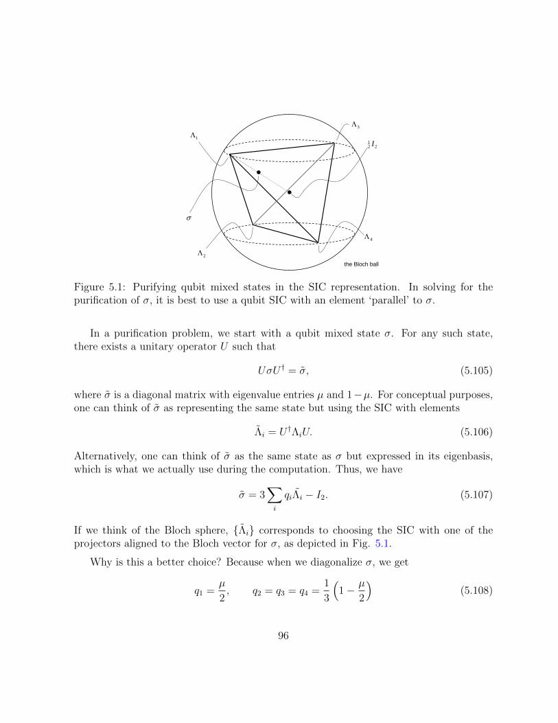
σ

the Bloch ball

221 I

1Λ

2Λ

3Λ

4Λ

Figure 5.1: Purifying qubit mixed states in the SIC representation. In solving for thepurification of σ, it is best to use a qubit SIC with an element ‘parallel’ to σ.

In a purification problem, we start with a qubit mixed state σ. For any such state,there exists a unitary operator U such that

UσU † = σ, (5.105)

where σ is a diagonal matrix with eigenvalue entries µ and 1−µ. For conceptual purposes,one can think of σ as representing the same state but using the SIC with elements

Λi = U †ΛiU. (5.106)

Alternatively, one can think of σ as the same state as σ but expressed in its eigenbasis,which is what we actually use during the computation. Thus, we have

σ = 3∑i

qiΛi − I2. (5.107)

If we think of the Bloch sphere, {Λi} corresponds to choosing the SIC with one of theprojectors aligned to the Bloch vector for σ, as depicted in Fig. 5.1.

Why is this a better choice? Because when we diagonalize σ, we get

q1 =µ

2, q2 = q3 = q4 =

1

3

(1− µ

2

)(5.108)

96

where µ and 1− µ are the eigenvalues of σ. To be consistent with {Λi}, we should definethe purification ρ in terms of the ququart SIC Πi = V †ΠiV ,

ρ = 516∑i=1

piΠi − I4. (5.109)

where V = U ⊗ I2.

One systematic way to solve this would be to let

v1 = p1 + p3 − p6 − p8,

v2 = p5 + p7 − p2 − p4,

v3 = p9 + p11 − p13 − p15,

v4 = p14 + p16 − p10 − p12. (5.110)

Using the partial trace equations for this particular choice of SICs, the conditions forobtaining the purification ~p are

v1 = −v2,

v4 = −v3, (5.111)

v1 − v4 =(−5 + 3

√5)(4µ− 2)

10(√

10− 2√

2)− 5(−1 +

√5)3/2

subject to constraints in Eq. (5.104). Because the structure coefficients αijk are quitenon-trivial, this appears to be the best simplification we can achieve.

5.8 Entanglement in 2-qubit systems

Entanglement is considered to be one of the defining characteristics of quantum phenomena.Parts of an entangled system exhibit strong correlations that cannot be achieved by anyclassical system and these correlations can be observed even when the parts are separatedat arbitrarily large distances. A 1935 paper by Albert Einstein, Boris Podolsky, and NathanRosen is often cited as the originator of the idea of quantum entanglement, where theyused it in an argument that was supposed to demonstrate the inadequacy of quantummechanics, known widely as the EPR paradox. Here we examine the entanglement of2-qubit systems in the SIC representation.

97

Consider two quantum systems A and B with states on Hilbert spaces HA and HB,respectively. The composite system AB has states on the tensor product Hilbert spaceHA ⊗HB, which just means that if {|ai〉} is an orthonormal basis for HA and {|bj〉} is anorthonormal basis for HB, then the vectors |ai, bj〉 ≡ |ai〉 ⊗ |bj〉 constitute an orthonormalbasis for HAB.

We say that |ψ〉 is a separable state of HAB if there exists |ψA〉 ∈ HA and |ψB〉 ∈ HB

such that|ψ〉 = |ψA〉 ⊗ |ψB〉 . (5.112)

Otherwise, the state is entangled. More generally, a density operator ρAB onHAB is deemedseparable if it can be expressed as

ρAB =∑i

piρiA ⊗ ρiB (5.113)

where ρiA and ρiB are states on subsystems A and B, respectively. In other words, ρAB isseparable if it is probability distribution over product states for the composite system. Aquantum state is said to be entangled if it is not separable in this more general sense.

In quantum information theory, an entanglement witness is an geometric object thatcan be evaluated for quantum states and whose values distinguish an entangled state fromseparable ones. Deciding whether an arbitrary quantum state is separable or not is a highlynontrivial problem especially when one extends to multipartite case. However, we will justfocus on a specific result for bipartite systems due to Asher Peres, and the Horodecki trioof Micha l, Pawe l, and Ryzard.

The Peres-Horodecki criterion [88, 105] gives a necessary condition for the separabilityof a joint density operator ρAB ∈ B(HA ⊗HB) that depends only on the positivity of itspartial transpose. In the case where systems A and B are both qubits or one is a qubitwhile the other is a qutrit, then it is also a sufficient condition. For those 2 situations, itprovides a definitive test for entanglement in mixed states.

The theorem is stated as follows: For any state ρ ∈ B(HA ⊗HB),

ρ =∑i,j,k,l

ωijkl |i〉 〈j| ⊗ |k〉 〈l| (5.114)

the partial transpose with respect to system B is defined by

ρTB =∑i,j,k,l

ωijkl |i〉 〈j| ⊗ (|k〉 〈l|)T =∑i,j,k,l

ωijkl |i〉 〈j| ⊗ |l〉 〈k|. (5.115)

98

The partial transpose with respect to system A is defined similarly. If ρ is separable thenρTB is positive definite (same for ρTA). Thus, if ρTB has negative eigenvalues, ρ is necessarilyentangled.

It is instructive to consider two examples involving 2-qubit states. The first exampleinvolves density operators of the form

ρ = q|ψ1〉〈ψ1|+ (1− q)|ψ2〉〈ψ2| (5.116)

where

|ψ1〉 = a |e1〉 ⊗ |e1〉+ b |e2〉 ⊗ |e2〉 ,|ψ2〉 = a |e1〉 ⊗ |e2〉+ b |e2〉 ⊗ |e1〉 , (5.117)

for a, b > 0 and some orthonormal basis {|e1〉 , |e2〉} ⊂ C2. Such states have been consideredin the study of Bell inequalities.

We can write out ρ and its partial transpose in matrix form using the basis {|ei〉⊗|ej〉}.

ρ =

qa2 0 0 qab

0 (1− q)a2 (1− q)ab 0

0 (1− q)ab (1− q)b2 0

qab 0 0 qb2

, (5.118)

ρTB =

qa2 0 0 (1− q)ab0 (1− q)a2 qab 0

0 qab (1− q)b2 0

(1− q)ab 0 0 qb2

. (5.119)

To check for the positivity of ρTB , we only need to consider two principal minors or deter-minants, since for Hermitian operators, positive semi-definiteness is guaranteed if all theprincipal minors are non-negative:

D1 =

∣∣∣∣∣ qa2 (1− q)ab(1− q)ab qb2

∣∣∣∣∣ , D2 =

∣∣∣∣∣ (1− q)a2 qab

qab (1− q)b2

∣∣∣∣∣ = −D1. (5.120)

We can easily see that

D1 = a2b2[q2 − (1− q)2] = a2b2(2q − 1). (5.121)

99

Thus, for ab 6= 0, q 6= 12, either D1 or D2 is negative. When q = 1

2, ρTB = ρ.

What would the criterion look like when states are represented using SICs? In termsof a ququart SIC {Πi}16

i=1,

ρ =∑i

(5p(i)− 1

4

)Πi. (5.122)

Substituting the ρ in Eq. (5.118), we find that∑i

p(i)2 =1

10

(1− q + q2

)(5.123)

in which case q = 12

corresponds to a right-hand side of 340

. Therefore, for this particularfamily of states, the SIC probability distributions p(i) such that

3

40<∑i

p(i)2 ≤ 1

10(5.124)

are associated with entangled 2-qubit states.

The other example we consider are Werner states

ρ = q|Ψ−〉〈Ψ−|+(

1− q4

)I4 (5.125)

where |Ψ−〉 = (|01〉 − |10〉)/√

2 is the singlet state. These states can be thought of asmixtures of a Bell state with the completely mixed state.

In the computational basis, ρ and its partial transpose are given by

ρ =1

4

1− q 0 0 0

0 1 + q −2q 0

0 −2q 1 + q 0

0 0 0 1− q

,

ρTB =1

4

1− q 0 0 −2q

0 1 + q 0 0

0 0 1 + q 0

−2q 0 0 1− q

. (5.126)

100

It is straightforward to calculate the eigenvalues of ρTB , which are

1

4(1− 3q),

1 + q

4,1 + q

4,1 + q

4. (5.127)

The first one is the smallest one for any 0 ≤ q ≤ 1 and it is non-negative only when q ≤ 13.

Thus, ρ of Eq. (5.126) is entangled for q > 13. Expressing the Werner state in Eq. (5.125)

in the SIC representation, we get∑i

p(i)2 =1

80

(5 + 3q2

). (5.128)

Hence, the Werner state ρ is entangled with respect to the product basis for two qubitswhen

1

15<∑i

p(i)2 ≤ 1

10. (5.129)

In general, we can consider the linear operator

H = (d+ 1)∑i

piΠi − I, (5.130)

with d = 4 and the set {Πi}16i=1 is a ququart SIC. When ~p is a probability vector, H

is necessarily a unit trace Hermitian operator. To be a density operator, H must also bepositive semidefinite, which can be enforced using a lemma first stated by Gen Kimura [78]:

Lemma 5.8.1. Consider the monic polynomial of degree d ≥ 1

f(x) =d∑j=0

(−1)jajxd−j =

d∏i=1

(x− xi) (5.131)

where a0 = 1 and which has only real roots xi ∈ R, i = 1, 2, ..., d when f(x) = 0. Then forall the roots xi to be positive semidefinite, all coefficients ai must be positive semidefinite,and vice-versa:

∀i, xi ≥ 0 ⇐⇒ ai ≥ 0. (5.132)

Applying the lemma to the characteristic polynomial of H, we get the desired positivityconstraints using Newton-Girard identities that relate coefficients of a monic polynomial

101

with the sums of powers of its roots [72]:

a1 = Tr (H) = 1, (5.133)

a2 =1

2

(1− Tr

(H2))≥ 0, (5.134)

a3 =1

6

(1− 3Tr

(H2)

+ 2Tr(H3))≥ 0, (5.135)

a4 =1

24

(1− 6Tr

(H4)

+ 8Tr(H3)− 6Tr

(H2)

+ 3Tr(H2)2)≥ 0. (5.136)

where the coefficients aj refer to the characteristic polynomial of H, defined to be consistentwith Eq. (5.131).

In terms of SICs, it is easy to verify that

Tr(H2)

= d(d+ 1)∑i

p2i − 1,

Tr(H3)

= d(d+ 1)2∑i,j,k

Sijkpipjpk − 2d(d+ 1)∑i

p2i + 1,

Tr(H4)

= d(d+ 1)3∑

i,j,k,l,m

SijmSklmpipjpkpl − 4d(d+ 1)2∑i,j,k

Sijkpipjpk

+ d2(d+ 1)

(∑i

p2i

)2

+ 4d(d+ 1)∑i

p2i − 1, (5.137)

where Sijk are the structure coefficients for the ququart SIC, which leads to the followingpositivity conditions on H:

a1 = 1,

a2 = 1− d(d+ 1)

2

∑i

p2i ≥ 0,

a3 =1

6

[6− 7d(d+ 1)

∑i

p2i + 2d(d+ 1)2

∑i,j,k

Sijkpipjpk

]≥ 0.

a4 =1

24

(24− 6d(d+ 1)3

∑i,j,k,l,m

SijmSklmpipjpkpl + 32d(d+ 1)2∑i,j,k

Sijkpipjpk

+ (3(d+ 1)− 6)d2(d+ 1)

(∑i

p2i

)2

− 52d(d+ 1)∑i

p2i

)≥ 0. (5.138)

102

Since this result works for any hermitian operator, it can also be applied to the partialtranspose of H, in which case the Peres-Horodecki criterion tells us that H corresponds toa separable state if and only if the coefficients ai for HTB are all non-negative.

5.9 Quantum operations as affine maps on SIC prob-

abilities

An important topic in the study of quantum information processing involves the studyof quantum operations, particularly maps of density operators that describe open-systemevolution. Studying such maps is useful for various applications such as developing methodsin quantum control or for identifying new witnesses for quantum entanglement. [91], MarkByrd et al., provide a description of general maps of density operators in terms of affinemaps of the corresponding Bloch vector representation of quantum states. In this section,we provide a similar description using the SIC representation.

Let the Kraus decomposition for a general (completely positive) map between densityoperators ρ, ρ′ of the same dimension be given by

Φ(ρ) =r∑i=1

AiρA†i = ρ′ (5.139)

where Ai are the Kraus operators. Note that if the map is trace preserving then

r∑i=1

A†iAi = I. (5.140)

What we want is to get the corresponding description in terms of a linear or affine map onSIC probability vectors. In this case, we write density operators in terms of the SIC Πi,

ρ =d2∑i=1

[(d+ 1)pi −

1

d

]Πi. (5.141)

Because SICs form a basis for the space of operators, we can do the same for the Krausoperators

Ai =d2∑j=1

aijΠj. (5.142)

103

Two special classes of maps to consider are unital and trace-preserving maps. If Φ isunital then Φ(I) = I. Translating in terms of SICs,

r∑i=1

AiA†i =

r∑i=1

d2∑j,k=1

aija∗ikΠjΠk

=r∑i=1

d2∑j,k,l=1

aija∗ikSjklΠl = I (5.143)

where we used the structure coefficients,

ΠjΠk =d2∑l=1

SjklΠl. (5.144)

Because∑d2

l=1 Πl = dI for SICs, we obtain that for any l

r∑i=1

d2∑j,k=1

aija∗ikSjkl =

1

d. (5.145)

Observe that the trace-preserving condition in Eq. (5.140) reads

r∑i=1

d2∑j,k=1

a∗ijaikSjkl =1

d. (5.146)

Moreover, from Tr (Φ(ρ)) = Tr (ρ) = 1, we get

r∑i=1

d2∑j,k,l=1

aijqka∗ilTjkl = 1 (5.147)

where we used the triple products

Tjkl = Tr (ΠjΠkΠl) (5.148)

and

qk = (d+ 1)pk −1

d. (5.149)

104

In general,

Φ(ρ) =r∑i=1

∑j,k,l

aijqka∗ilΠjΠkΠl (5.150)

Let ΠjΠk =∑

m SjkmΠm and ΠmΠl =∑

n SmlnΠn. Then

Φ(ρ) =r∑i=1

d2∑j,k,l=1

d2∑m,n=1

aijqka∗ilSjkmSmlnΠn =

d2∑n=1

[r∑i=1

d2∑j,k,l,m=1

aijqka∗ilSjkmSmln

]Πn.

(5.151)

Thus, Eq. (5.151) says that ρ 7→ Φ(ρ) corresponds to the linear map

qn 7→ q′n =r∑i=1

d2∑j,k,l,m=1

aijqka∗ilSjkmSmln, (5.152)

that is, each component of ~q given by Eq. (5.149) gets mapped to another vector given interms of the expansion coefficients of the Kraus operators and the structure coefficients.

Writing it out explicitly, we have

q′n = (d+ 1)r∑i=1

d2∑j,k,l,m=1

aijpka∗ilSjkmSmln −

1

d

r∑i=1

d2∑j,k,l,m=1

aija∗ilSjkmSmln. (5.153)

If the map in Eq. (5.152) is unital then we can write the second term above as

1

d

r∑i=1

d2∑j,l,m=1

aija∗ilSmlndδjm =

r∑i=1

d2∑j,l=1

aija∗ilSjln =

1

d. (5.154)

where we used∑

k Sjkm = dδjm and Eq. (5.145). This says that if the map is unital thenthe map applies to the probability vector ~p directly:

pn 7→ p′n =r∑i=1

d2∑j,k,l,m=1

aijpka∗ilSjkmSmln. (5.155)

Of course, Eq. (5.145) will not be true for non-unital maps so generally we would get anaffine map ~p 7→ ~p′ = M~p+ ~t where

Mjk =r∑i=1

d2∑l,m,n=1

aima∗inSmklSlnj, tj =

1

d(d+ 1)

(1−

d2∑k=1

Mjk

). (5.156)

The following are some examples of simple maps for density operators:

105

1. Trace-preserving inversion map:

ρ 7→ 1

d− 1(I − ρ) . (5.157)

For pure states, this maps |ψ〉 to some state orthogonal to |ψ〉. We have

ρ 7→ 1

d− 1

[I − (d+ 1)

∑i

piΠi + I

]

=∑i

[2

d(d− 1)− d+ 1

d− 1pi

]Πi

≡∑i

[(d+ 1)p′i −

1

d

]Πi, (5.158)

which implies that

p′i =1

d− 1

(1

d− pi

). (5.159)

For instance, if we consider the SIC basis state

~p =

(1

d,

1

d(d+ 1), . . . ,

1

d(d+ 1)

)T, (5.160)

that is, the probability vector for ρ = Π1, then

~p′ =

(0,

1

d2 − 1, . . . ,

1

d2 − 1)

)T. (5.161)

This means that

~p · ~p′ = 1

d(d+ 1)(5.162)

which is indeed the value of the scalar product for orthogonal pure states.

2. Completely positive inversion map (approximate universal NOT gate):

ρ 7→ 1

d2 − 1(dI − ρ) . (5.163)

106

We have

ρ 7→ 1

d2 − 1

[dI + I − (d+ 1)

∑i

piΠi

]

=∑i

[1

d(d− 1)− pid− 1

]Πi

≡∑i

[(d+ 1)p′i −

1

d

]Πi, (5.164)

which implies that

p′i =1

d2 − 1(1− pi) . (5.165)

For instance, if we consider the SIC basis state in Eq. (5.160) then

~p′ =

(1

d(d+ 1),

d2 + d− 1

d(d− 1)(d+ 1)2, . . . ,

d2 + d− 1

d(d− 1)(d+ 1)2

)T. (5.166)

3. Trace-preserving projection onto a random (average) pure state:

ρ 7→ 1

d+ 1(I + ρ) . (5.167)

We have

ρ 7→ 1

d+ 1

[I + (d+ 1)

∑i

piΠi − I

]=∑i

piΠi

≡∑i

[(d+ 1)p′i −

1

d

]Πi, (5.168)

which implies that

p′i =1

d+ 1

(pi +

1

d

). (5.169)

For instance, if we consider the SIC basis state in Eq. (5.160) then

~p′ =

(2

d(d+ 1),

d+ 2

d(d+ 1)2, . . . ,

d+ 2

d(d+ 1)2

)T. (5.170)

107

4. Qudit depolarizing channel:

ρ 7→ (1− ε)ρ+ε

dI. (5.171)

We have

ρ 7→ (1− ε)

[(d+ 1)

∑i

piΠi − I

]+ε

dI

= (1− ε)

[(d+ 1)

∑i

piΠi

]−(

1− ε− ε

d

)I

=

[(d+ 1)pi(1− ε)−

1

d

(1− (d+ 1)ε

d

)]Πi

≡∑i

[(d+ 1)p′i −

1

d

]Πi, (5.172)

which implies that

p′i = (1− ε)pi +ε

d2. (5.173)

For instance, if we consider the SIC basis state in Eq. (5.160) then

~p′ =

(d(1− ε) + ε

d2,

d+ ε

d2(d+ 1), . . . ,

d+ ε

d2(d+ 1)

)T. (5.174)

5. Qudit flip channel:

ρ 7→d−1∑i=0

εiXiρX i† (5.175)

where εi represents the probability of |j〉 7→ |j ⊕ i〉 for the orthonormal basis {|j〉}d−1j=0

that is shifted by X,X |j〉 = |j ⊕ 1〉 (5.176)

with i ⊕ j = i + j mod d and later, i j = i − j mod d. In this example, it isconvenient to restrict ourselves to Weyl-Heisenberg SICs,

|ψjk〉 = XjZk |ψ〉 , Πjk = |ψjk〉〈ψjk| (5.177)

so the relation between density operators and probability vectors can be written as

ρ =d−1∑j,k=0

(d+ 1)pjkΠjk − I. (5.178)

108

Thus,

ρ 7→d−1∑i=0

d−1∑j,k=0

εi [(d+ 1)pjk]XiΠjkX

i† −d−1∑i=0

εiXiX i†

= (d+ 1)d−1∑i=0

d−1∑j,k=0

εipjkΠ(j⊕i)k − I

= (d+ 1)d−1∑i=0

d−1∑j,k=0

εip(ji)kΠjk − I, (5.179)

which implies that

p′jk =d−1∑i=0

εip(ji)k. (5.180)

For instance, if εi = 1d

for all i and we consider the SIC basis state

pjk =dδj0δk0 + 1

d(d+ 1)(5.181)

then

p′jk =

2

d(d+ 1)if k = 0,

1

d(d+ 1)if k 6= 0.

(5.182)

6. Qutrit phase damping channel:

ρ 7→ (1− ε)ρ+ εZρZ† (5.183)

where

Z =

1 0 0

0 ω 0

0 0 ω2

(5.184)

and ω = ei2π3 . Here we consider Weyl-Heisenberg SICs generated from the vectors

|ψjk〉 = X iZj |ψ〉 (5.185)

109

where

X =

0 0 1

1 0 0

0 1 0

(5.186)

and |ψ〉 is some fiducial vector. Writing the density operator as

ρ =2∑

j,k=0

(d+ 1)pjkΠjk − I (5.187)

and~p =

(p00, p01, p02, p10, p11, p12, p20, p21, p22

)T, (5.188)

it is straightforward to show that ~p 7→M~p where

M =

B 0 0

0 B 0

0 0 B

, B =

1− ε 0 ε

ε 1− ε 0

0 ε 1− ε

. (5.189)

7. Qutrit amplitude damping channel, with Kraus operators

A1 =

1 0 0

0√

1− ε 0

0 0√

1− ε

, A2 =

0√ε 0

0 0 0

0 0 0

, A3 =

0 0√ε

0 0 0

0 0 0

, (5.190)

where ε = 1−e−Γt represents the decoherence parameter. We can compute the affinemap directly from these matrices Ai if we express them as

Ai =3∑

j,k=1

AijkEjk (5.191)

where Ejk are just the standard basis matrices

E11 =

1 0 0

0 0 0

0 0 0

, E12 =

0 1 0

0 0 0

0 0 0

, . . . , E33 =

0 0 0

0 0 0

0 0 1

. (5.192)

110

We can then compute aim in Eq. (5.156) using

ail =∑j,k

AijkTr (EjkDl) . (5.193)

where Dl is the dual operator to the SIC projector Πl

Dl =1

3(4Πl − I) . (5.194)

We can choose any qutrit SIC for computing the structure coefficients, which mightbe tedious but is straightforward. We find that the affine map ~p 7→ M~p + ~t for theamplitude damping noise is given by

M =1

3

B1 −B2 −B2

B2 B3 B2

B2 B2 B3

(5.195)

where

B1 =

3− 4ε −ε −ε−ε 3− 4ε −ε−ε −ε 3− 4ε

, B2 =

ε ε εε ε ε

ε ε ε

, B3 =

1 + 2ε′ 1− ε′ 1− ε′

1− ε′ 1 + 2ε′ 1− ε′

1− ε′ 1− ε′ 1 + 2ε′

,

(5.196)

with ε′ =√

1− ε, and

~t =1

6

2~v

−~v−~v

, ~v =

εεε

. (5.197)

111

Chapter 6

Geometric features of qutrit statespace

A qutrit is any 3-level quantum system whose pure states are described by unit vectors|ψ〉 ∈ H3. More generally, a qutrit is described by a density operator

ρ =1

3I + τ (6.1)

where τ is a traceless Hermitian matrix that makes ρ positive semidefinite.

Analogous to the Bloch ball representation for qubits, states for qutrits are often de-scribed using 8 linearly independent generators of SU(3), also known as the Gell-Mannmatrices λi. We can express any qutrit density operator ρ in terms of λi and I,

ρ =1

3

(I +√

3∑i

riλi

), (6.2)

where a pure state corresponds to some unit vector ~r ∈ R8 on a 7-dimensional sphere.

The convex set of all qutrit states is such that it contains an in-sphere of radius r andis inscribed by an out-sphere of radius R, where the radii of the 2 spheres are related by

r

R=

1

2. (6.3)

In this chapter, we identify several interesting geometric properties of qutrit state spacein terms of SIC probability vectors.

112

6.1 Qutrit pure states in terms of SICs

Harkening back to some of our results in Chapter 3 and Chapter 5, we will now describethe pure states of a qutrit in terms of SICs. It is useful to recall the general case∑

i

p(i)2 =1

d(d+ 1)(6.4)

∑i,j,k

Sijkp(i)p(j)p(k) =4

d(d+ 1)2(6.5)

where Sijk are the real parts of the structure coefficients for the Lie algebra defined bythe basis of SIC operators. Thinking about the probability vectors ~p as points in an affinespace, the former condition defines the sphere containing pure states while the latter con-dition picks out the points on that sphere that actually correspond to quantum states. Asmentioned before, the set of points that describe d-dimensional pure states is topologicallyidentical to the points in complex projective space CPd+1.

Specializing to the case d = 3, a SIC probability vector ~p corresponds to a qutrit purestate if and only if ∑

i

p(i)2 =1

6,

∑i,j,k

Sijkp(i)p(j)p(k) =1

12. (6.6)

A particularly elegant formula for pure states is obtained by considering the mostexceptional SIC, which is the Weyl-Heisenberg SIC with fiducial vector

|ψ0〉 =1√2

0

1

−1

. (6.7)

The probability distributions ~p for the most exceptional SIC are given by∑i

p(i)2 =1

6, (6.8)

1

3

∑i

p(i)3 =∑

(ijk)∈Q

p(i)p(j)p(k) (6.9)

113

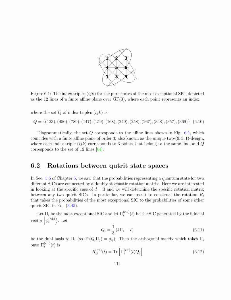
9 8 7

6 5 4

3 2 1

Figure 6.1: The index triples (ijk) for the pure states of the most exceptional SIC, depictedas the 12 lines of a finite affine plane over GF(3), where each point represents an index.

where the set Q of index triples (ijk) is

Q = {(123), (456), (789), (147), (159), (168), (249), (258), (267), (348), (357), (369)} (6.10)

Diagrammatically, the set Q corresponds to the affine lines shown in Fig. 6.1, whichcoincides with a finite affine plane of order 3, also known as the unique two-(9, 3, 1)-design,where each index triple (ijk) corresponds to 3 points that belong to the same line, and Qcorresponds to the set of 12 lines [64].

6.2 Rotations between qutrit state spaces

In Sec. 5.5 of Chapter 5, we saw that the probabilities representing a quantum state for twodifferent SICs are connected by a doubly stochastic rotation matrix. Here we are interestedin looking at the specific case of d = 3 and we will determine the specific rotation matrixbetween any two qutrit SICs. In particular, we can use it to construct the rotation Rt

that takes the probabilities of the most exceptional SIC to the probabilities of some otherqutrit SIC in Eq. (3.45).

Let Πi be the most exceptional SIC and let Π(r±)i (t) be the SIC generated by the fiducial

vector∣∣∣ψ(r±)

t

⟩. Let

Qi =1

3(4Πi − I) (6.11)

be the dual basis to Πi (so Tr(QiΠj) = δij). Then the orthogonal matrix which takes Πi

onto Π(r±)i (t) is

R(r±)ij (t) = Tr

[Π

(r±)i (t)Qj

](6.12)

114

It turns out that the matrices R(r±)(t) have a very simple form. Define the permutations

p(0+) =

(1 2 3 4 5 6 7 8 9

1 2 3 4 5 6 7 8 9

), p(0−) =

(1 2 3 4 5 6 7 8 9

1 3 2 4 6 5 7 9 8

),

p(1+) =

(1 2 3 4 5 6 7 8 9

1 5 9 2 6 7 3 4 8

), p(1−) =

(1 2 3 4 5 6 7 8 9

1 9 5 2 7 6 3 8 4

),

p(2+) =

(1 2 3 4 5 6 7 8 9

1 6 8 2 4 9 3 5 7

), p(2−) =

(1 2 3 4 5 6 7 8 9

1 8 6 2 9 4 3 7 5

),

p(3+) =

(1 2 3 4 5 6 7 8 9

1 4 7 2 5 8 3 6 9

), p(3−) =

(1 2 3 4 5 6 7 8 9

1 7 4 2 8 5 3 9 6

). (6.13)

Let P (r±) be the permutation matrix corresponding to p(r±), with matrix elements

P(r±)ij = δj,p(r±)(i). (6.14)

Also define

a(t) =1

3(1 + 2 cos 2t), (6.15)

A(t) =

a(t) a(t− π

3

)a(t+ π

3

)a(t+ π

3

)a(t) a

(t− π

3

)a(t− π

3

)a(t+ π

3

)a(t)

, (6.16)

R(t) =

A(t) 0 0

0 A(t) 0

0 0 A(t)

. (6.17)

It is then straightforward, though somewhat tedious, to verify that

R(r±)(t) =[P (r±)

]−1R(t)P (r±). (6.18)

Since R(t) = I ⊗ A(t), it follows that

Det[R(r±)(t)

]= Det[R(t)] = {Det [A(t)]}3 . (6.19)

Because A(t) is a circulant matrix, its eigenvalues are given by

λm = a(t) + ωma(t− π

3

)+ ω−ma

(t+

π

3

)= e2itm (6.20)

115

for m = −1, 0, 1. This implies that Det [A(t)] = 1. Thus, Det[R(r±)(t)

]= 1 and R(r±)(t)

is, in fact, a rotation matrix.

It is easily seen that

R(t1)R(t2) = R(t1 + t2), R(0) = I. (6.21)

So the matrices R(t) form a 1-parameter subgroup of the orthogonal group.

We have just established how the qutrit state spaces of different qutrit SICs are relatedby 3-dimensional rotations. It suggests a particular symmetry of the probability statespace in d = 3 that we identify in the next section.

6.3 A permutation symmetry for qutrit pure states

Having established the rotational equivalence of the probability spaces for different qutritSICs, we can now ask the question, what are the symmetry properties possessed by theconvex body of qutrits? For comparison, we know that the unitary symmetry for qubitscorresponds to the spherical symmetry for the convex body of qubits, which is most ap-parent in the Bloch representation. We would like to gain a similar insight into the morecomplicated geometry of qutrits.

Because of the results of the previous section, we know we can focus our attention onthe probabilities for most exceptional SIC, whose cubic condition for pure states given byEq. (6.6) already implies a certain kind of permutation symmetry, which we attempt tomake more explicit. To do so, it is better to consider the pure-state condition ρ = ρ2,which in SIC terms is just

p(k) =(d+ 1)

3

∑i,j

Sijkp(i)p(j) +2

3d(d+ 1)(6.22)

for k = 1, 2, . . . , d2. For the most exceptional SIC, Eq. (6.22) becomes

12p(k)2 − 6p(k)− 12∑

(ijk)∈Q

p(i)p(j) + 1 = 0, (6.23)

116

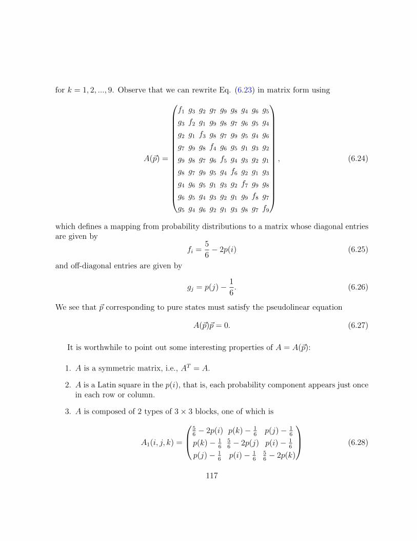
for k = 1, 2, ..., 9. Observe that we can rewrite Eq. (6.23) in matrix form using

A(~p) =

f1 g3 g2 g7 g9 g8 g4 g6 g5

g3 f2 g1 g9 g8 g7 g6 g5 g4

g2 g1 f3 g8 g7 g9 g5 g4 g6

g7 g9 g8 f4 g6 g5 g1 g3 g2

g9 g8 g7 g6 f5 g4 g3 g2 g1

g8 g7 g9 g5 g4 f6 g2 g1 g3

g4 g6 g5 g1 g3 g2 f7 g9 g8

g6 g5 g4 g3 g2 g1 g9 f8 g7

g5 g4 g6 g2 g1 g3 g8 g7 f9

, (6.24)

which defines a mapping from probability distributions to a matrix whose diagonal entriesare given by

fi =5

6− 2p(i) (6.25)

and off-diagonal entries are given by

gj = p(j)− 1

6. (6.26)

We see that ~p corresponding to pure states must satisfy the pseudolinear equation

A(~p)~p = 0. (6.27)

It is worthwhile to point out some interesting properties of A = A(~p):

1. A is a symmetric matrix, i.e., AT = A.

2. A is a Latin square in the p(i), that is, each probability component appears just oncein each row or column.

3. A is composed of 2 types of 3× 3 blocks, one of which is

A1(i, j, k) =

56− 2p(i) p(k)− 1

6p(j)− 1

6

p(k)− 16

56− 2p(j) p(i)− 1

6

p(j)− 16

p(i)− 16

56− 2p(k)

(6.28)

117

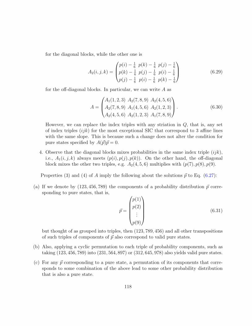
for the diagonal blocks, while the other one is

A2(i, j, k) =

p(i)−16p(k)− 1

6p(j)− 1

6

p(k)− 16p(j)− 1

6p(i)− 1

6

p(j)− 16p(i)− 1

6p(k)− 1

6

(6.29)

for the off-diagonal blocks. In particular, we can write A as

A =

A1(1, 2, 3) A2(7, 8, 9) A2(4, 5, 6)

A2(7, 8, 9) A1(4, 5, 6) A2(1, 2, 3)

A2(4, 5, 6) A2(1, 2, 3) A1(7, 8, 9)

. (6.30)

However, we can replace the index triples with any striation in Q, that is, any setof index triples (ijk) for the most exceptional SIC that correspond to 3 affine lineswith the same slope. This is because such a change does not alter the condition forpure states specified by A(~p)~p = 0.

4. Observe that the diagonal blocks mixes probabilities in the same index triple (ijk),i.e., A1(i, j, k) always meets (p(i), p(j), p(k)). On the other hand, the off-diagonalblock mixes the other two triples, e.g. A2(4, 5, 6) multiplies with (p(7), p(8), p(9).

Properties (3) and (4) of A imply the following about the solutions ~p to Eq. (6.27):

(a) If we denote by (123, 456, 789) the components of a probability distribution ~p corre-sponding to pure states, that is,

~p =

p(1)

p(2)...

p(9)

(6.31)

but thought of as grouped into triples, then (123, 789, 456) and all other transpositionsof such triples of components of ~p also correspond to valid pure states.

(b) Also, applying a cyclic permutation to each triple of probability components, such astaking (123, 456, 789) into (231, 564, 897) or (312, 645, 978) also yields valid pure states.

(c) For any ~p corresponding to a pure state, a permutation of its components that corre-sponds to some combination of the above lead to some other probability distributionthat is also a pure state.

118

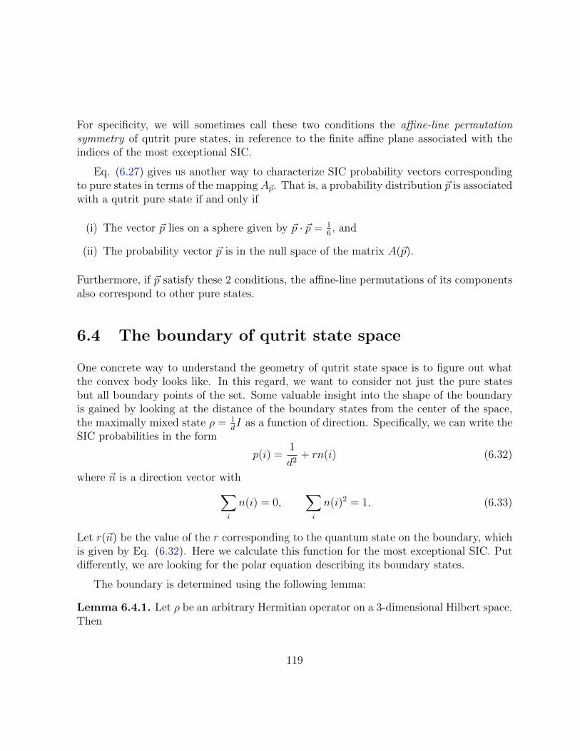
For specificity, we will sometimes call these two conditions the affine-line permutationsymmetry of qutrit pure states, in reference to the finite affine plane associated with theindices of the most exceptional SIC.

Eq. (6.27) gives us another way to characterize SIC probability vectors correspondingto pure states in terms of the mapping A~p. That is, a probability distribution ~p is associatedwith a qutrit pure state if and only if

(i) The vector ~p lies on a sphere given by ~p · ~p = 16, and

(ii) The probability vector ~p is in the null space of the matrix A(~p).

Furthermore, if ~p satisfy these 2 conditions, the affine-line permutations of its componentsalso correspond to other pure states.

6.4 The boundary of qutrit state space

One concrete way to understand the geometry of qutrit state space is to figure out whatthe convex body looks like. In this regard, we want to consider not just the pure statesbut all boundary points of the set. Some valuable insight into the shape of the boundaryis gained by looking at the distance of the boundary states from the center of the space,the maximally mixed state ρ = 1

dI as a function of direction. Specifically, we can write the

SIC probabilities in the form

p(i) =1

d2+ rn(i) (6.32)

where ~n is a direction vector with∑i

n(i) = 0,∑i

n(i)2 = 1. (6.33)

Let r(~n) be the value of the r corresponding to the quantum state on the boundary, whichis given by Eq. (6.32). Here we calculate this function for the most exceptional SIC. Putdifferently, we are looking for the polar equation describing its boundary states.

The boundary is determined using the following lemma:

Lemma 6.4.1. Let ρ be an arbitrary Hermitian operator on a 3-dimensional Hilbert space.Then

119

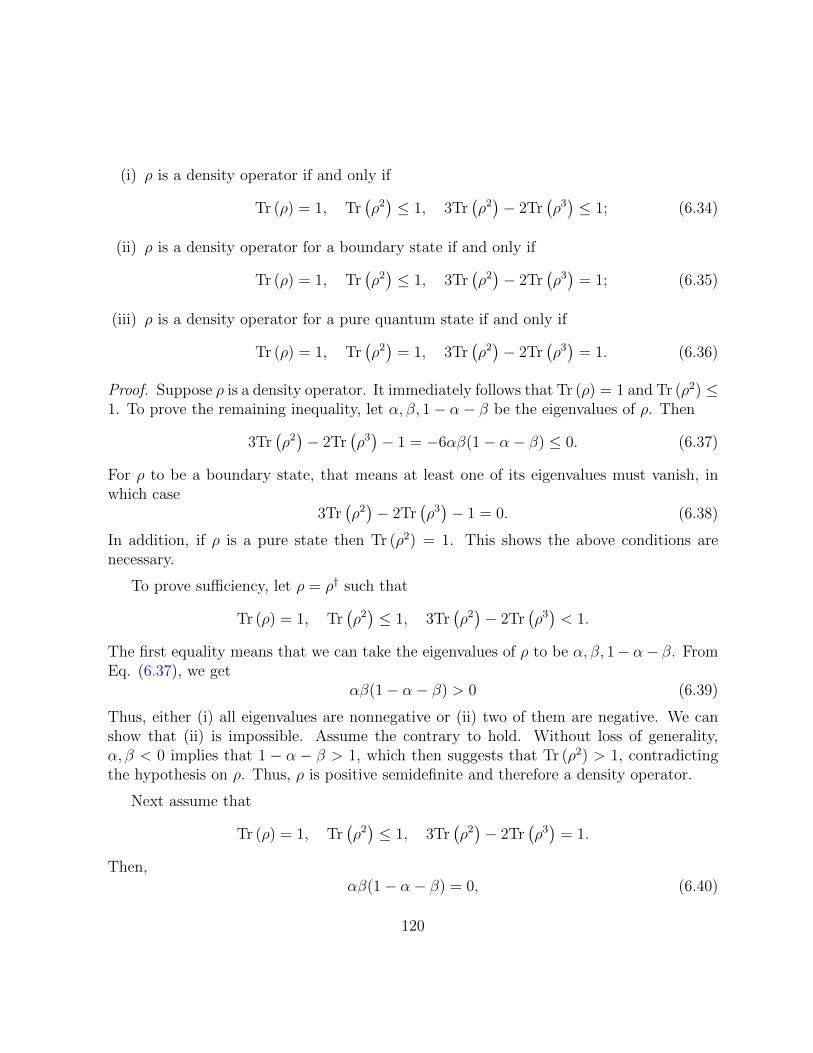
(i) ρ is a density operator if and only if

Tr (ρ) = 1, Tr(ρ2)≤ 1, 3Tr

(ρ2)− 2Tr

(ρ3)≤ 1; (6.34)

(ii) ρ is a density operator for a boundary state if and only if

Tr (ρ) = 1, Tr(ρ2)≤ 1, 3Tr

(ρ2)− 2Tr

(ρ3)

= 1; (6.35)

(iii) ρ is a density operator for a pure quantum state if and only if

Tr (ρ) = 1, Tr(ρ2)

= 1, 3Tr(ρ2)− 2Tr

(ρ3)

= 1. (6.36)

Proof. Suppose ρ is a density operator. It immediately follows that Tr (ρ) = 1 and Tr (ρ2) ≤1. To prove the remaining inequality, let α, β, 1− α− β be the eigenvalues of ρ. Then

3Tr(ρ2)− 2Tr

(ρ3)− 1 = −6αβ(1− α− β) ≤ 0. (6.37)

For ρ to be a boundary state, that means at least one of its eigenvalues must vanish, inwhich case

3Tr(ρ2)− 2Tr

(ρ3)− 1 = 0. (6.38)

In addition, if ρ is a pure state then Tr (ρ2) = 1. This shows the above conditions arenecessary.

To prove sufficiency, let ρ = ρ† such that

Tr (ρ) = 1, Tr(ρ2)≤ 1, 3Tr

(ρ2)− 2Tr

(ρ3)< 1.

The first equality means that we can take the eigenvalues of ρ to be α, β, 1− α− β. FromEq. (6.37), we get

αβ(1− α− β) > 0 (6.39)

Thus, either (i) all eigenvalues are nonnegative or (ii) two of them are negative. We canshow that (ii) is impossible. Assume the contrary to hold. Without loss of generality,α, β < 0 implies that 1 − α − β > 1, which then suggests that Tr (ρ2) > 1, contradictingthe hypothesis on ρ. Thus, ρ is positive semidefinite and therefore a density operator.

Next assume that

Tr (ρ) = 1, Tr(ρ2)≤ 1, 3Tr

(ρ2)− 2Tr

(ρ3)

= 1.

Then,αβ(1− α− β) = 0, (6.40)

120

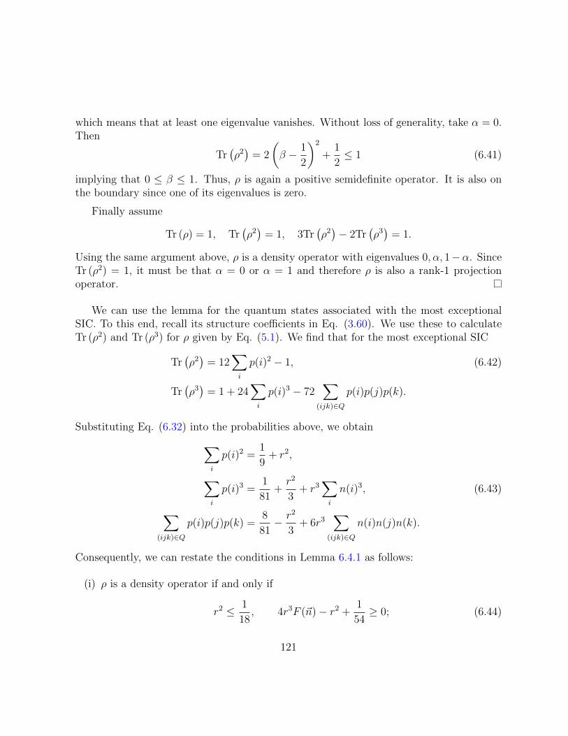
which means that at least one eigenvalue vanishes. Without loss of generality, take α = 0.Then

Tr(ρ2)

= 2

(β − 1

2

)2

+1

2≤ 1 (6.41)

implying that 0 ≤ β ≤ 1. Thus, ρ is again a positive semidefinite operator. It is also onthe boundary since one of its eigenvalues is zero.

Finally assume

Tr (ρ) = 1, Tr(ρ2)

= 1, 3Tr(ρ2)− 2Tr

(ρ3)

= 1.

Using the same argument above, ρ is a density operator with eigenvalues 0, α, 1−α. SinceTr (ρ2) = 1, it must be that α = 0 or α = 1 and therefore ρ is also a rank-1 projectionoperator.

We can use the lemma for the quantum states associated with the most exceptionalSIC. To this end, recall its structure coefficients in Eq. (3.60). We use these to calculateTr (ρ2) and Tr (ρ3) for ρ given by Eq. (5.1). We find that for the most exceptional SIC

Tr(ρ2)

= 12∑i

p(i)2 − 1, (6.42)

Tr(ρ3)

= 1 + 24∑i

p(i)3 − 72∑

(ijk)∈Q

p(i)p(j)p(k).

Substituting Eq. (6.32) into the probabilities above, we obtain∑i

p(i)2 =1

9+ r2,

∑i

p(i)3 =1

81+r2

3+ r3

∑i

n(i)3, (6.43)

∑(ijk)∈Q

p(i)p(j)p(k) =8

81− r2

3+ 6r3

∑(ijk)∈Q

n(i)n(j)n(k).

Consequently, we can restate the conditions in Lemma 6.4.1 as follows:

(i) ρ is a density operator if and only if

r2 ≤ 1

18, 4r3F (~n)− r2 +

1

54≥ 0; (6.44)

121

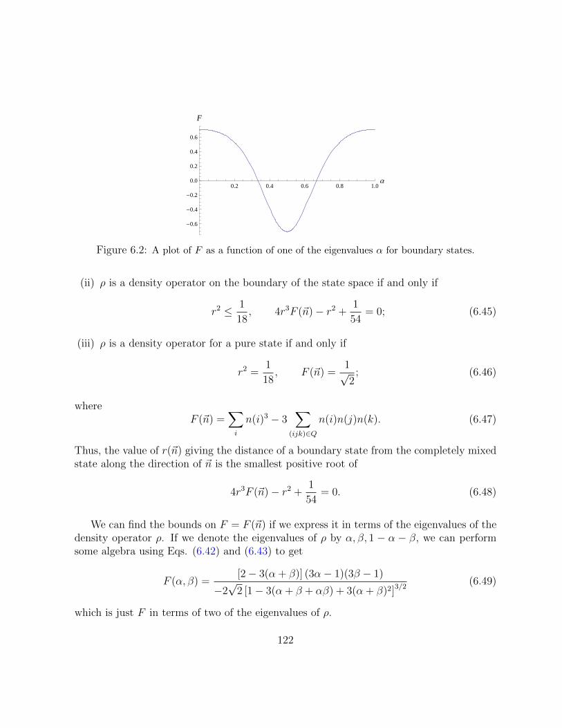
0.2 0.4 0.6 0.8 1.0Α

-0.6

-0.4

-0.2

0.0

0.2

0.4

0.6

F

Figure 6.2: A plot of F as a function of one of the eigenvalues α for boundary states.

(ii) ρ is a density operator on the boundary of the state space if and only if

r2 ≤ 1

18, 4r3F (~n)− r2 +

1

54= 0; (6.45)

(iii) ρ is a density operator for a pure state if and only if

r2 =1

18, F (~n) =

1√2

; (6.46)

whereF (~n) =

∑i

n(i)3 − 3∑

(ijk)∈Q

n(i)n(j)n(k). (6.47)

Thus, the value of r(~n) giving the distance of a boundary state from the completely mixedstate along the direction of ~n is the smallest positive root of

4r3F (~n)− r2 +1

54= 0. (6.48)

We can find the bounds on F = F (~n) if we express it in terms of the eigenvalues of thedensity operator ρ. If we denote the eigenvalues of ρ by α, β, 1 − α − β, we can performsome algebra using Eqs. (6.42) and (6.43) to get

F (α, β) =[2− 3(α + β)] (3α− 1)(3β − 1)

−2√

2 [1− 3(α + β + αβ) + 3(α + β)2]3/2(6.49)

which is just F in terms of two of the eigenvalues of ρ.

122

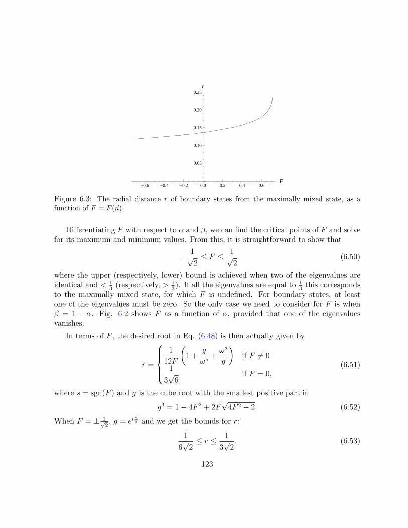
-0.6 -0.4 -0.2 0.0 0.2 0.4 0.6F

0.05

0.10

0.15

0.20

0.25r

Figure 6.3: The radial distance r of boundary states from the maximally mixed state, as afunction of F = F (~n).

Differentiating F with respect to α and β, we can find the critical points of F and solvefor its maximum and minimum values. From this, it is straightforward to show that

− 1√2≤ F ≤ 1√

2(6.50)

where the upper (respectively, lower) bound is achieved when two of the eigenvalues areidentical and < 1

3(respectively, > 1

3). If all the eigenvalues are equal to 1

3this corresponds

to the maximally mixed state, for which F is undefined. For boundary states, at leastone of the eigenvalues must be zero. So the only case we need to consider for F is whenβ = 1 − α. Fig. 6.2 shows F as a function of α, provided that one of the eigenvaluesvanishes.

In terms of F , the desired root in Eq. (6.48) is then actually given by

r =

1

12F

(1 +

g

ωs+ωs

g

)if F 6= 0

1

3√

6if F = 0,

(6.51)

where s = sgn(F ) and g is the cube root with the smallest positive part in

g3 = 1− 4F 2 + 2F√

4F 2 − 2. (6.52)

When F = ± 1√2, g = ei

π3 and we get the bounds for r:

1

6√

2≤ r ≤ 1

3√

2. (6.53)

123

A plot of r as a function of F is shown in Fig. 6.3.

6.5 Plane sections of qutrit state space

To be able to visualize the shape of qutrit state space, we need to go beyond just analgebraic description of its boundary. Since we are unable to plot it as a subset of R9,the best we can do is look at lower-dimensional cross-sections of the space. A number ofauthors [56,68,78,79,97] have previously explored 2-dimensional and 3-dimensional cross-sections of the generalized Bloch representation of a qutrit. Here we review some of theirresults and compare it with what one would get for the SIC representation.

For Hilbert spaces of dimension two, it is convenient to represent the set of quantumstates on a Bloch ball. There are two main reasons why Bloch vectors provide an elegantrepresentation for quantum states:

(i) Every quantum state is represented by a real-valued vector whose components referto expectation values of some minimal informationally-complete measurement.

(ii) The dynamics of a quantum system is manifested by intuitive operations on the Blochball—for example, unitary evolution corresponds to a rotations of the ball, while adepolarizing quantum channel corresponds to shrinking the ball radius.

We can extend the notion of a Bloch sphere in higher dimensions by using the infinitesimalgenerators of the special unitary group SU(d) as the generalization of Pauli matrices, whichis a set of d2 − 1 operators λi that together with the identity operator form an orthogonalbasis for d× d complex matrices. The generalized Bloch vector space for d > 2 is a propersubset of a ball in Rd2−1.

Any density operator ρ can then be written as

ρ =1

d

(I +

d

2~r · ~λ

), (6.54)

where ~λ is a vector of the generators of SU(d) and ~r is the generalized Bloch vector. Inhigher dimensions, not all of the points on the surface of the sphere correspond to purestates. The simplest way to explain the discrepancy is to say that vectors ~r that do notcorrespond to positive semidefinite ρ are excluded since they do not describe quantumstates. In essence, the richness in the geometric structure of quantum state space is aconsequence of positivity.

124

To establish the required constraints on ρ, we employ once again Lemma 5.8.1 inSec. 5.8, which when applied to the characteristic polynomial of Eq. (6.54) leads to thefollowing theorem:

Theorem 6.5.1. Let ai(~r) be the coefficients of the characteristic polynomial det(xI − ρ)of ρ and define the Bloch vector space B,

B(Rd2−1

)= {~r ∈ Rd2−1 | ai(~r) ≥ 0}. (6.55)

Then the map

~r ∈ B(Rd2−1

)7→ ρ =

1

d

(I +

d

2~r · ~λ

)∈ D, (6.56)

is a bijection from B(Rd2−1

)to the density operator space D.

The positivity conditions ai(~r) ≥ 0 can then be expressed in terms of trace powers ofρ using the Newton-Girard identities. Specializing to d = 3, the theorem says that ρ ispositive semidefinite when

a1 = Tr (ρ) = 1,

a2 =1− Tr (ρ2)

2≥ 0, (6.57)

a3 =1− 3Tr (ρ2) + 2Tr (ρ3)

6≥ 0.

Kimura [78] provides a nice visualization of qutrit states by plotting the 2-dimensionalsections of the generalized Bloch vector space. In this section, we compare those planesections with the ones obtained for SIC probability vectors.

Recall the density operator expressed in terms of SIC probabilities,

ρ =∑i

[(d+ 1)p(i)− 1

d

]Πi. (6.58)

We simply plug in this ρ into the positivity conditions of Eq. (6.57). By definition, a1 =Tr (ρ) = 1 for a density operator. For the constraint a2(~p) ≥ 0 we have

a2(~p) = 1− d(d+ 1)

2

∑i

p(i)2 ≥ 0. (6.59)

125

On the other hand, for a3(~p) ≥ 0 we have

a3(~p) =1

6

[6− 7d(d+ 1)

∑i

p(i)2 + 2d(d+ 1)2∑i,j,k

Sijkp(i)p(j)p(k)

]≥ 0. (6.60)

Note that the pure states correspond to the case a2 = 0 and a3 = 0. We can then comparethe 2-dimensional sections for the SIC probability vectors with the cross-sections

S2(i, j) = {~r ∈ B(R8)|~r = (0, ..., ri, 0, ..., rj, ..., 0)} (6.61)

obtained by Kimura for Bloch vectors [78]. It is helpful to know the mapping from ~r to ~pobtained from equating Eq. (6.54) and Eq. (6.58),

1

3I +

1

2~r · ~λ = 4~p · ~Π− I, (6.62)

where ~Π is the vector of SIC projectors of the most exceptional SIC. One way to work thisout explicitly is to expand each SIC element in terms of the basis defined by the Gell-Mannmatrices and the identity operator. The cross-sections S2(i, j) expressed in terms of SICprobabilities are listed in Table 6.1 and shown in Fig. 6.4.

Samples of each type of 2-dimensional cross-section are displayed in Fig. 6.4. It isimportant to note that these plane sections are identical to Kimura’s graphs [78] if plot-ted with respect to the two parameters defining each subspace. This is consistent withRosado’s observation that the set of Bloch vectors and the set of SIC probability vec-tors corresponding to quantum states are identical, up to an appropriately chosen scalingfactor [114].

Such 2-dimensional qutrit sections have been considered before and here we brieflyrevisit some of the observations made by previous authors regarding the unitary equivalenceof cross-sections.

There are a total of 8C2 = 28 plane sections to consider, where a general 2-dimensionalcross-section corresponds to density operators of the form

ρ =1

3(I + xλ1 + yλ2) (6.63)

where λ1, λ2 are traceless hermitian operators and x, y ∈ R. Two 2-dimensional cross-sections are said to be unitarily equivalent if for some unitary operator U in SU(3),

(Uλ1u†, Uλ2U

†) = (λ1, λ2) (6.64)

126

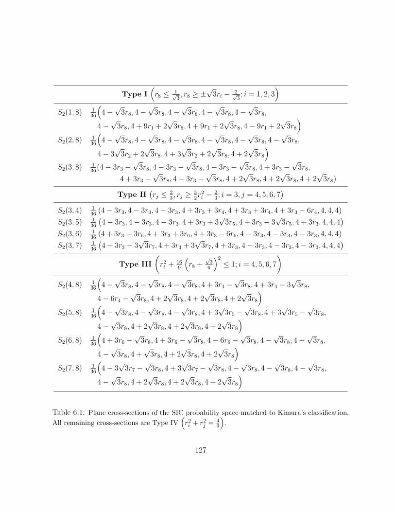
Type I(r8 ≤ 1√

3, r8 ≥ ±

√3ri − 2√

3; i = 1, 2, 3

)S2(1, 8) 1

36

(4−√

3r8, 4−√

3r8, 4−√

3r8, 4−√

3r8, 4−√

3r8,

4−√

3r8, 4 + 9r1 + 2√

3r8, 4 + 9r1 + 2√

3r8, 4− 9r1 + 2√

3r8

)S2(2, 8) 1

36

(4−√

3r8, 4−√

3r8, 4−√

3r8, 4−√

3r8, 4−√

3r8, 4−√

3r8,

4− 3√

3r2 + 2√

3r8, 4 + 3√

3r2 + 2√

3r8, 4 + 2√

3r8

)S2(3, 8) 1

36(4− 3r3 −

√3r8, 4− 3r3 −

√3r8, 4− 3r3 −

√3r8, 4 + 3r3 −

√3r8,

4 + 3r3 −√

3r8, 4− 3r3 −√

3r8, 4 + 2√

3r8, 4 + 2√

3r8, 4 + 2√

3r8)

Type II(rj ≤ 2

3, rj ≥ 3

2r2i − 2

3; i = 3, j = 4, 5, 6, 7

)S2(3, 4) 1

36(4− 3r3, 4− 3r3, 4− 3r3, 4 + 3r3 + 3r4, 4 + 3r3 + 3r4, 4 + 3r3 − 6r4, 4, 4, 4)

S2(3, 5) 136

(4− 3r3, 4− 3r3, 4− 3r3, 4 + 3r3 + 3

√3r5, 4 + 3r3 − 3

√3r5, 4 + 3r3, 4, 4, 4

)S2(3, 6) 1

36(4 + 3r3 + 3r6, 4 + 3r3 + 3r6, 4 + 3r3 − 6r6, 4− 3r3, 4− 3r3, 4− 3r3, 4, 4, 4)

S2(3, 7) 136

(4 + 3r3 − 3

√3r7, 4 + 3r3 + 3

√3r7, 4 + 3r3, 4− 3r3, 4− 3r3, 4− 3r3, 4, 4, 4

)Type III

(r2i + 16

9

(r8 +

√3

6

)2

≤ 1; i = 4, 5, 6, 7

)S2(4, 8) 1

36

(4−√

3r8, 4−√

3r8, 4−√

3r8, 4 + 3r4 −√

3r8, 4 + 3r4 − 3√

3r8,

4− 6r4 −√

3r8, 4 + 2√

3r8, 4 + 2√

3r8, 4 + 2√

3r8

)S2(5, 8) 1

36

(4−√

3r8, 4−√

3r8, 4−√

3r8, 4 + 3√

3r5 −√

3r8, 4 + 3√

3r5 −√

3r8,

4−√

3r8, 4 + 2√

3r8, 4 + 2√

3r8, 4 + 2√

3r8

)S2(6, 8) 1

36

(4 + 3r6 −

√3r8, 4 + 3r6 −

√3r8, 4− 6r6 −

√3r8, 4−

√3r8, 4−

√3r8,

4−√

3r8, 4 +√

3r8, 4 + 2√

3r8, 4 + 2√

3r8

)S2(7, 8) 1

36

(4− 3

√3r7 −

√3r8, 4 + 3

√3r7 −

√3r8, 4−

√3r8, 4−

√3r8, 4−

√3r8,

4−√

3r8, 4 + 2√

3r8, 4 + 2√

3r8, 4 + 2√

3r8

)

Table 6.1: Plane cross-sections of the SIC probability space matched to Kimura’s classification.

All remaining cross-sections are Type IV(r2i + r2

j = 49

).

127

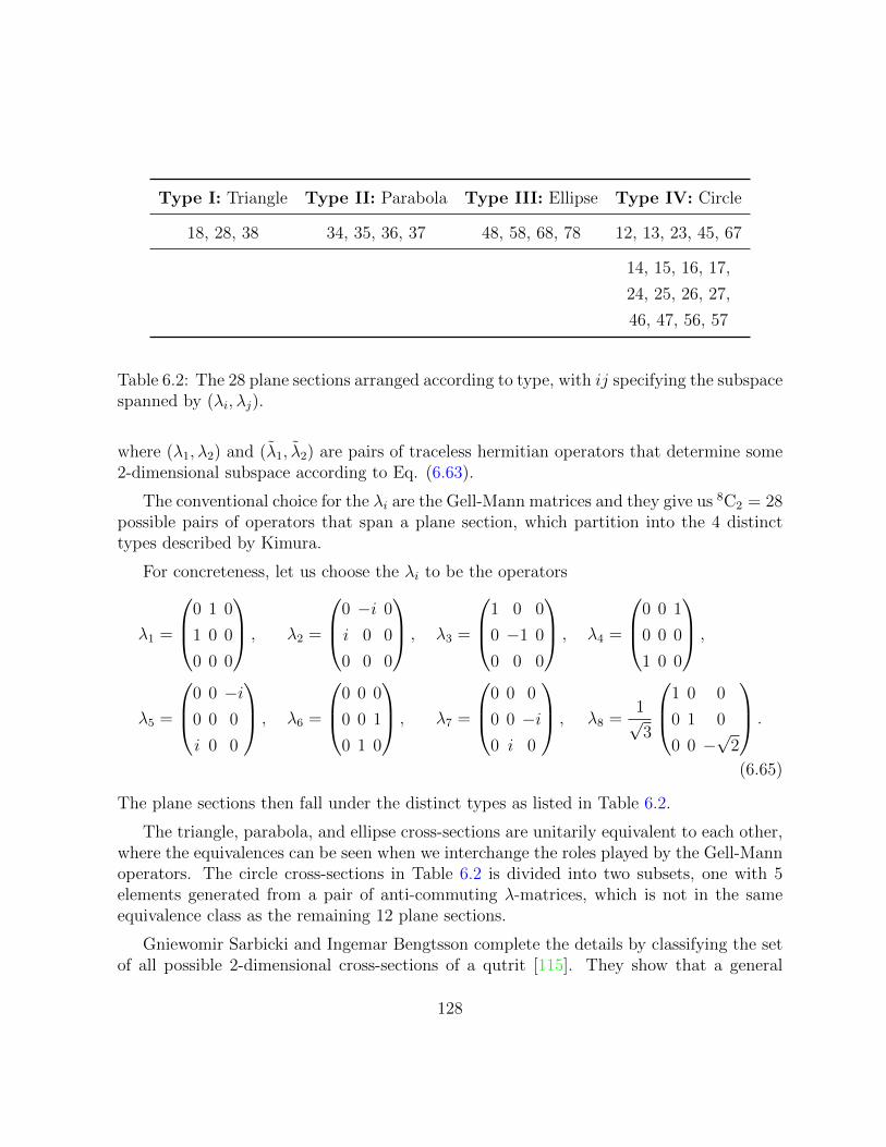
Type I: Triangle Type II: Parabola Type III: Ellipse Type IV: Circle

18, 28, 38 34, 35, 36, 37 48, 58, 68, 78 12, 13, 23, 45, 67

14, 15, 16, 17,

24, 25, 26, 27,

46, 47, 56, 57

Table 6.2: The 28 plane sections arranged according to type, with ij specifying the subspacespanned by (λi, λj).

where (λ1, λ2) and (λ1, λ2) are pairs of traceless hermitian operators that determine some2-dimensional subspace according to Eq. (6.63).

The conventional choice for the λi are the Gell-Mann matrices and they give us 8C2 = 28possible pairs of operators that span a plane section, which partition into the 4 distincttypes described by Kimura.

For concreteness, let us choose the λi to be the operators

λ1 =

0 1 0

1 0 0

0 0 0

, λ2 =

0 −i 0

i 0 0

0 0 0

, λ3 =

1 0 0

0 −1 0

0 0 0

, λ4 =

0 0 1

0 0 0

1 0 0

,

λ5 =

0 0 −i0 0 0

i 0 0

, λ6 =

0 0 0

0 0 1

0 1 0

, λ7 =

0 0 0

0 0 −i0 i 0

, λ8 =1√3

1 0 0

0 1 0

0 0 −√

2

.

(6.65)

The plane sections then fall under the distinct types as listed in Table 6.2.

The triangle, parabola, and ellipse cross-sections are unitarily equivalent to each other,where the equivalences can be seen when we interchange the roles played by the Gell-Mannoperators. The circle cross-sections in Table 6.2 is divided into two subsets, one with 5elements generated from a pair of anti-commuting λ-matrices, which is not in the sameequivalence class as the remaining 12 plane sections.

Gniewomir Sarbicki and Ingemar Bengtsson complete the details by classifying the setof all possible 2-dimensional cross-sections of a qutrit [115]. They show that a general

128

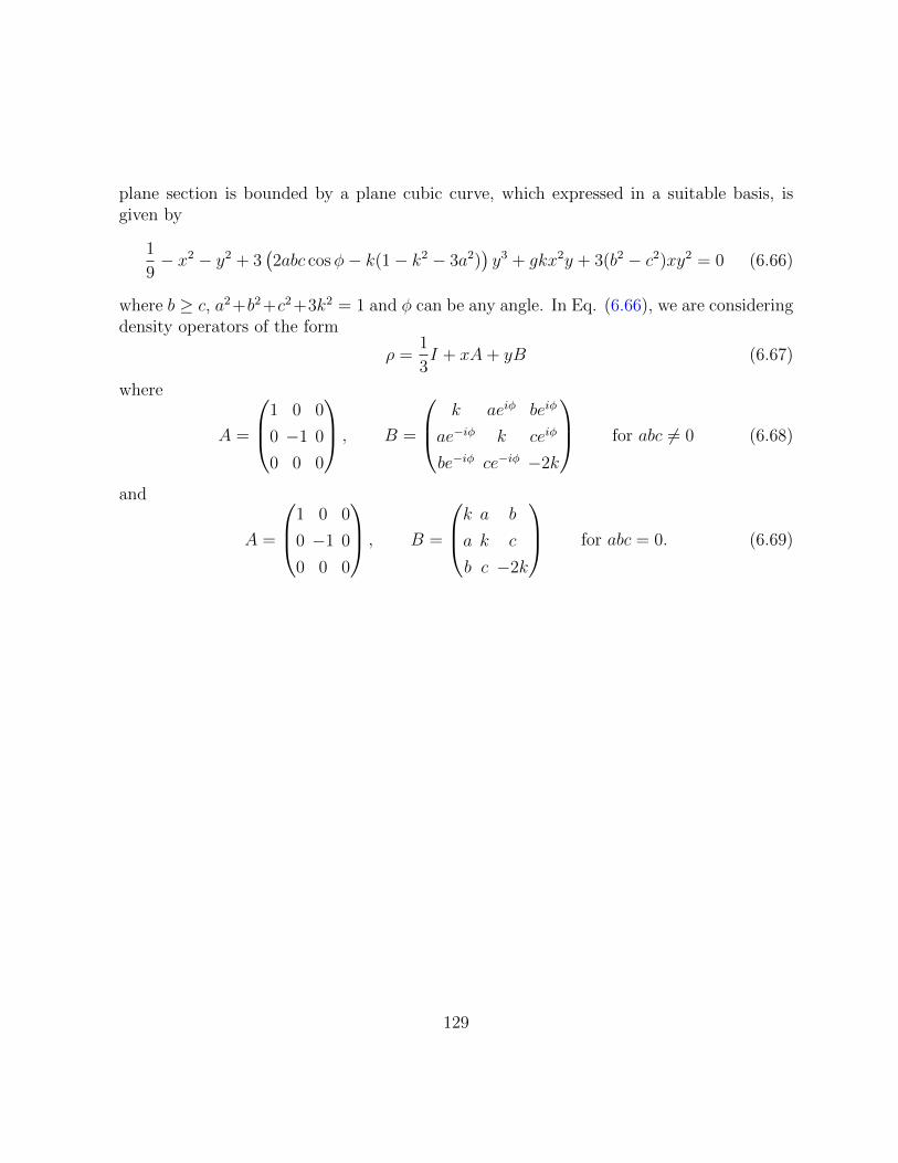
plane section is bounded by a plane cubic curve, which expressed in a suitable basis, isgiven by

1

9− x2 − y2 + 3

(2abc cosφ− k(1− k2 − 3a2)

)y3 + gkx2y + 3(b2 − c2)xy2 = 0 (6.66)

where b ≥ c, a2 +b2 +c2 +3k2 = 1 and φ can be any angle. In Eq. (6.66), we are consideringdensity operators of the form

ρ =1

3I + xA+ yB (6.67)

where

A =

1 0 0

0 −1 0

0 0 0

, B =

k aeiφ beiφ

ae−iφ k ceiφ

be−iφ ce−iφ −2k

for abc 6= 0 (6.68)

and

A =

1 0 0

0 −1 0

0 0 0

, B =

k a b

a k c

b c −2k

for abc = 0. (6.69)

129

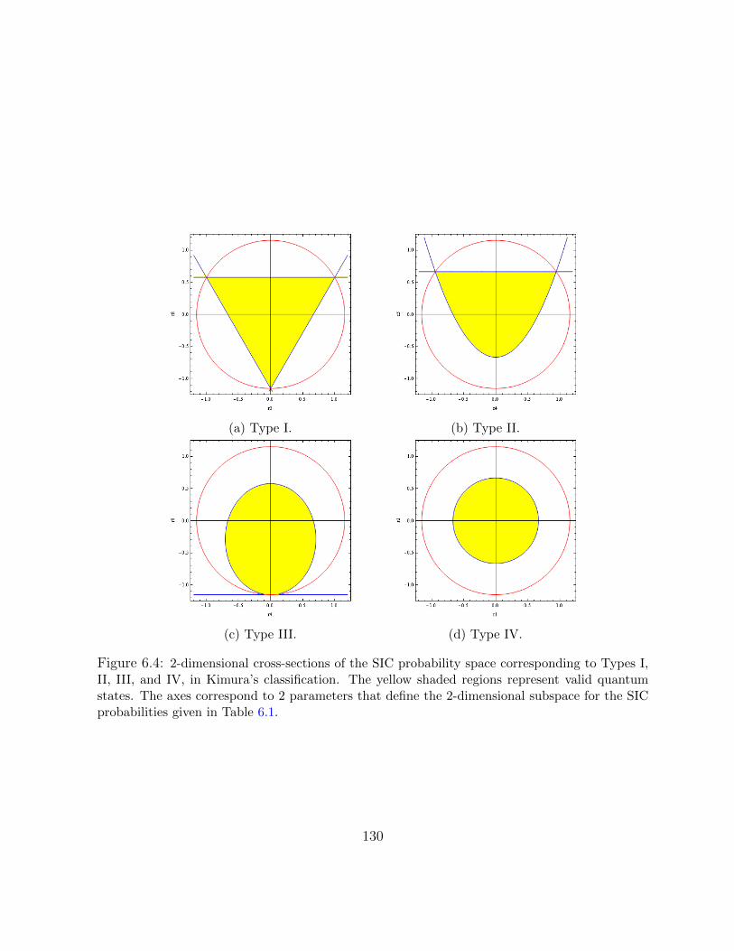
(a) Type I. (b) Type II.

(c) Type III. (d) Type IV.

Figure 6.4: 2-dimensional cross-sections of the SIC probability space corresponding to Types I,II, III, and IV, in Kimura’s classification. The yellow shaded regions represent valid quantumstates. The axes correspond to 2 parameters that define the 2-dimensional subspace for the SICprobabilities given in Table 6.1.

130

Chapter 7

Quantum state space as a maximalconsistent set

The Born rule specifies the probabilities for the outcome of any quantum measurement.In the SIC representation where states and measurements are expressed in terms of a SIC{Π}d2i=1,

q(j) =∑i

[(d+ 1)p(i)− 1

d

]r(j|i) (7.1)

expresses the probability of result j for some measurement {Ej}Nj=1 described by the con-ditional probabilities

r(j|i) = Tr (EjΠi) . (7.2)

At first glance, Eq. (7.1) looks like an affine transformation

p(i) 7→ (d+ 1)p(i)− 1

d(7.3)

on the probabilities. This hints at the intriguing possibility that quantum theory can beunderstood as some type of extension of classical probability theory that includes certainevents that require a different rule for relating marginal to conditional probabilities.

If we think of the Born rule as such an extension, it implies that quantum mechanicscorresponds to a restriction on the probability simplex ∆d2−1 ⊂ Rd2 , since not all possiblep(i) or r(j|i) will yield a valid probability distribution for q(j). In fact, some of theconstraints implied by the Born rule can be expressed in terms of a set of inequalities,which we will use to define the notion of maximal consistency, and which will serve as thejumping-off point for our efforts to reconstruct quantum state space.

131

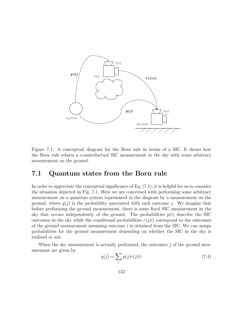
SIC

Any

sky

ground

p(i) r(j|i)

q(j)

system

Figure 7.1: A conceptual diagram for the Born rule in terms of a SIC. It shows howthe Born rule relates a counterfactual SIC measurement in the sky with some arbitrarymeasurement on the ground.

7.1 Quantum states from the Born rule

In order to appreciate the conceptual significance of Eq. (7.1), it is helpful for us to considerthe situation depicted in Fig. 7.1. Here we are concerned with performing some arbitrarymeasurement on a quantum system represented in the diagram by a measurement on theground, where q(j) is the probability associated with each outcome j. We imagine thatbefore performing the ground measurement, there is some fixed SIC measurement in thesky that occurs independently of the ground. The probabilities p(i) describe the SICoutcomes in the sky while the conditional probabilities r(j|i) correspond to the outcomesof the ground measurement assuming outcome i is obtained from the SIC. We can assignprobabilities for the ground measurement depending on whether the SIC in the sky isrealized or not.

When the sky measurement is actually performed, the outcomes j of the ground mea-surement are given by

q(j) =∑i

p(j)r(j|i) (7.4)

132

in accordance with the usual laws of probability. This is how we would assign probabili-ties for a classical system. The quantum case corresponds to the scenario where the skymeasurement does not occur. In this case, the system is fed directly to the ground mea-surement and we use the Born rule in the form of Eq. (7.1), which expresses formally theidea that unperformed measurements have no outcomes.

Moreover, the similarity between Eq. (7.1) and Eq. (7.4) suggests that we may think ofthe Born rule as a certain kind of coherence condition on actual measurements done in thelaboratory with a counterfactual measurement, which we fix to be a SIC measurement, sothat quantum probabilities are not independent of the probabilities involved in Eq. (7.4)but are intimately connected to them.

Thus, if we would like to make the assumption that the Born rule constitutes a norma-tive addition to probability theory that leads to a formal description of quantum states interms of SIC probabilities, where we demand that

(i) the Born rule must yield q(j) that is a probability, and

(ii) using the Bayes’ rule on conditional probabilities lead to valid states.

To describe the actual conditions on the SIC probabilities in terms of inequalities, weobviously need (i) if we want to stay within the simplex while for (ii) we know that itshould at least hold in the case when we know both the ground and sky measurements areperformed but we are completely ignorant of the outcomes in the sky, that is, when

~p =1

d2

1...

1

(7.5)

then Bayes rule tells us that

r(i|j) =r(j|i)p(i)q(j)

=r(j|i)

(1d2

)∑k

(1d2

)r(j|k)

=r(j|i)∑k r(j|k)

≡ s(i) (7.6)

where it means that if we ignore the dependence on j, then the probability distribution ~smust correspond to a quantum state itself.

If we substitute Eq. (7.6) into Eq. (7.1) we have

q(j) =

[(d+ 1)

∑i

p(i)s(i)− 1

d

]∑k

r(j|k) (7.7)

133

Since q(j) ≥ 0 for ~q to be a proper probability distribution, we get

~p · ~s ≥ 1

d(d+ 1)(7.8)

where · is the usual scalar product for points in Rd2 . We can get an upper bound fromother considerations. For instance, one may take the special case of the sky measurementbeing the same as the ground measurement, in which case,

p(j) = (d+ 1)∑i

p(i)r(j|i)− 1

d

∑i

r(j|i), (7.9)

where r(j|i) denotes the same measurement for the ground and sky. Furthermore, wedemand that whenever we assign a uniform distribution for the sky measurement, we shouldassign a uniform distribution for the ground, a property called in-step unpredictability [47].So with p(i) = p(j) = 1

d2, we get ∑

i

r(j|i) = 1. (7.10)

We can use this special case in Eq. (7.7) and the constraint q(j) ≤ 1 gives us

~p · ~s ≤ 2

d(d+ 1). (7.11)

The same upper bound can be obtained by demanding that one can have at most d pointsin any set S where the dot product of any pair of probability vectors in S is equal to thelower bound 1

d(d+1)(in Hilbert space, the set S will just be an orthonormal basis).

Thus, we have1

d(d+ 1)≤ ~p · ~s ≤ 2

d(d+ 1)(7.12)

Because we do not specify any particular ~p or ~s, this condition must hold for any pair ofSIC probabilities that represent quantum states. And because it establishes a necessarybinary relation between quantum states, we refer to Eq. (7.12) as the consistency conditionfor SIC probabilities.

Since Eq. (7.12) is a constraint on SIC probabilities obtained from the Born rule, wecan start with the postulate that any probability distribution corresponding to a pure statemust satisfy this constraint. The remainder of the task, then, is to see what additionalstructure is needed in order to reconstruct the space of SIC probabilities isomorphic toquantum state space. Thus, we imagine the space of d-dimensional quantum states to be

134

a consistent subset of the d2 − 1 probability simplex, with a global geometric structurereflecting the projective unitary symmetry of the associated density operators.

So far, the constraints on the SIC probabilities from Eq. (7.12) just come from insistingthat ~q always be a probability vector. Without any other assumptions, the only other thingwe can demand is maximality. Suppose S is the set of probability vectors representingquantum states. S is said to maximal if it is the largest subset of the probability simplexthat is consistent. That is, if we consider any probability vector ~v 6∈ S, then for some ~p ∈ Sit must be the case that

~p · ~v < 1

d(d+ 1)or ~p · ~v > 2

d(d+ 1). (7.13)

Since S is both consistent and maximal, we refer to it as a maximal consistent set. Butbefore we describe our approach to reconstructing quantum state space as a maximalconsistent set, it is useful to consider some of the properties of any maximal consistentset. We do this in the next section by introducing a more general definition of maximalconsistent sets.

7.2 General maximal consistent sets

A more general notion of a maximal consistent set begins with identifying a normed realvector space V where the points are embedded in, also known as the ambient space. In thecase of SIC probabilities, this would be the probability simplex ∆d2−1 over d2 outcomes.In general, we consider any finite-dimensional real inner product space, which means V isisomorphic to some subset of the real Euclidean n-space equipped with its canonical innerproduct, the dot product

〈~p, ~q〉 = ~p · ~q =n∑i=1

piqi (7.14)

for any ~p, ~q ∈ Rn.

Consider some finite-dimensional real vector space V with inner product 〈p, q〉. Forsome constant k ∈ R, a subset S ⊂ V is said to be consistent if

〈p, q〉 ≥ k (7.15)

for all p, q ∈ S. As a matter of terminology, when 〈p, q〉 = k, p and q are said to bemaximally distant.

135

Observe that in this general definition of consistency, we omit the upper bound that ispart of the definition in Eq. (7.12). Later we will see that the upper bound can be madeto follow from a the boundedness of quantum state space [36].

A consistent set S ⊂ V is said to be maximal if it is not contained in any largerconsistent set in V , that is, for any r ∈ V but r 6∈ S, there is at least one q ∈ S such that

〈q, r〉 < k. (7.16)

In other words, no further points in V can be added to S without breaking its consis-tency. An alternate definition of maximality would be that for any consistent set S ′ ⊂ Vcontaining S must be identical to S, i.e.,

S ′ ⊇ S =⇒ S ′ = S. (7.17)

Next we consider some interesting examples of maximal consistent sets.

Example 7.2.1. Let V = Rn with the usual dot product and k = −1. The n-dimensionalunit ball centered at the origin

Bn = {~v ∈ V | ‖~v‖ ≤ 1} (7.18)

is a maximal consistent set.

Proof. To show that Bn is consistent, observe that since ‖~p‖ ≤ 1 for any point from theball, Cauchy-Schwarz inequality tells us that

〈~p, ~q〉 ≥ −‖~p‖‖~q‖ ≥ −1 (7.19)

for any ~p, ~q ∈ Bn.

To show that Bn is maximal, consider any ~r ∈ V but not in Bn. This must mean that‖~r‖ > 1. Now consider the vector

~q = − ~r

‖~r‖. (7.20)

Since

‖~q‖ =~q · ~q‖~q‖2

= 1 (7.21)

so ~q ∈ Bn. But

〈~q, ~r〉 = −~r · ~r‖~r‖

= −‖~r‖ < −1. (7.22)

Because ~q ∈ Bn for any ~r ∈ V not in the ball, Bn is not a proper subset of any consistentset in V . Thus, Bn is maximal.

136

Note that for antipodal points on the surface of the ball Bn,

~p = −~q, ‖~p‖ = 1 =⇒ 〈~p, ~q〉 = −1, (7.23)

so ~p and ~q give the lower bound. It is because of this that we call points that satisfy thelower bound maximally distant.

The next two examples show that physically interesting state spaces can be defined asmaximal consistent sets.

Example 7.2.2. Let V ⊂ Rn be the set of vectors ~v whose components in the standardbasis sum to zero,

n∑i=1

vi = 0. (7.24)

With the consistency condition

〈~v, ~w〉 = ~v · ~w = − 1

n(7.25)

the set

S =

{v ∈ V

∣∣∣ vi +1

n≥ 0

}(7.26)

forms a maximal consistent set. Observe that the vectors ~p

pi = vi +1

n(7.27)

is the set of n-dimensional probability distributions so S is effectively the space of classicalprobabilities (it is equal to the regular simplex up to a translation.)

Proof. To show that S is consistent, take ~v, ~w ∈ S. Since

vi +1

n≥ 0, wi +

1

n≥ 0, (7.28)

for all i, we haven∑i=1

(vi +

1

n

)(wi +

1

n

)≥ 0 (7.29)

137

Because the components of ~v and ~w sum to zero,

∑i

(vi +

1

n

)(wi +

1

n

)=∑i

viwi +1

n

(∑i

vi +∑i

wi

)+∑i

1

n2(7.30)

= 〈~v, ~w〉+1

n. (7.31)

Using inequality 7.29, this implies that

〈~v, ~w〉 ≥ − 1

n. (7.32)

Thus S is consistent.

To show that S is maximal, choose any ~u in V but not in S. For at least one componentof ~u, it must be the case that

ui +1

n< 0. (7.33)

Without loss of generality, suppose this holds for u1. Let ~v ∈ S be the vector withcomponents

vi = δ1i −1

n. (7.34)

This leads to

〈~u,~v〉 =

(1− 1

n

)u1 −

1

n

∑i 6=1

ui. (7.35)

Because ~u ∈ V , its components add to zero so

u1 = −∑i 6=1

ui (7.36)

and therefore,

〈~u,~v〉 =

(1− 1

n

)u1 −

1

nu1 = u1 < −

1

n. (7.37)

Thus, no set containing both ~u and ~v can be consistent. Since ~v ∈ S and ~u can be anyelement in V not in S this means that S is not contained in any larger consistent set in V .Therefore, S is maximal.

Example 7.2.3. Let V be the space of traceless Hermitian operators A on Cd,

A = A†, Tr (A) = 0 (7.38)

138

with inner product〈A,B〉 = Tr (AB) . (7.39)

With consistency given by

〈A,B〉 ≥ −1

d(7.40)

then the set

S =

{A ∈ V

∣∣∣ A+1

dI ≥ 0

}(7.41)

forms a maximal consistent set. Observe that if we take

ρ = A+1

dI (7.42)

for all A in S, we get the space of density operators, so S is effectively the set of quantumstates.

Proof. First, we show S is consistent. For any A,B ∈ S

Tr

[(A+

1

dI

)(A+

1

dI

)]≥ 0 (7.43)

since for any pair of positive semidefinite operators P,Q

Tr (PQ) ≥ 0. (7.44)

Because A and B are traceless, we have

Tr

[(A+

1

dI

)(A+

1

dI

)]= Tr (AB) +

1

d(Tr (A) + Tr (B)) +

1

d2Tr (I) (7.45)

= Tr (AB) +1

d(7.46)

which in conjunction with inequality 7.43 implies that

〈A,B〉 = Tr (AB) ≥ −1

d. (7.47)

Thus, S is consistent.

To show S is maximal, take any traceless Hermitian operator C not in S. Let {ej}nj=1

be an orthonormal basis in which C is diagonal, that is,

Cej = cj ej (7.48)

139

where cj is an eigenvalue of C.

Because C + 1dI is not positive semidefinite, at least one of the eigenvalues of C must

be less than −1d. Without loss of generality, suppose that c1 < −1

d. Let B ∈ S be the

operator given by the eigenvalue equations

Bej =

(δ1j −

1

d

)ej (7.49)

for j = 1, 2, ..., d. Observe that

〈B,C〉 = Tr (BC) =

(1− 1

d

)c1 −

1

d

∑j 6=1

cj (7.50)

Since Tr (C) = 0,

c1 = −∑j 6=1

cj (7.51)

and thus

〈B,C〉 =

(1− 1

d

)c1 +

1

dc1 = c1 < −

1

d. (7.52)

Because B ∈ S and C can be any element in V not in S, S does not belong to any largerconsistent set in V . Thus, S is maximal.

Example 7.2.4. Let V = Rn and choose some orthonormal basis E = {ej}nj=1 for V . Takethe usual scalar product with consistency given by

〈~p, ~q〉 = 0. (7.53)

The set

S =

{~p =

n∑i=1

piei

∣∣∣ pi ≥ 0

}(7.54)

forming the positive n-orthant of V in the basis E is a maximal consistent set [36].

Proof. To show S is consistent, let ~p, ~q ∈ V with nonnegative components in E. Then

〈~p, ~q〉 = ~p · ~q =∑i,j

piqj ei · ej =∑i

piqi ≥ 0 (7.55)

since pi, qi ≥ 0 for all i. Thus, S is consistent.

140

To show S is maximal, suppose that ~r is a vector with at least one of its coordinates isnegative. In that case,

〈~q, ~r〉 < 0 (7.56)

for at least one ~q ∈ E, that is, if we write ~r in coordinate form ~r = (r1, . . . , rn) then it willbe inconsistent with one of the vectors

(1, 0, . . . , 0), (0, 1, . . . , 0), . . . (0, 0, . . . , 1). (7.57)

Since these vectors are elements of the basis E and belong in S, and ~r can be any vectorin V that is not in S, then there is no larger consistent set in V that contains S. Thus, Sis maximal.

Example 7.2.5. Choose k > c > 0. Consider two concentric spheres of radii r < R where

r =c√k, R =

√k. (7.58)

Let u be some unit vector in V = Rn and

S =

{~p ∈ V

∣∣∣ ‖~p‖ = R, 〈~p, u〉 ≥√k − c

2

}T =

{− ck~p∣∣∣ ~p ∈ S} . (7.59)

Then the convex hull of S ∪ T is a maximal consistent set.

Proof. First we show that S ∪ T is consistent. The consistency of the convex hull followsfrom the property that the convex hull of any consistent set is consistent, which we provein Proposition 7.3.2.

Take any two points ~p, ~q ∈ S. We can express them in the form

~p = au+√k − a2v ~q = bu+

√k − b2w (7.60)

for unit vectors v and w orthogonal to u, that is, we can decompose ~p and ~q into componentsparallel and perpendicular to direction u. Since

〈~p, u〉 ≥√k − c

2, 〈~q, u〉 ≥

√k − c

2(7.61)

then

a ≥√k − c

2, b ≥

√k − c

2, =⇒ ab ≥ k − c

2. (7.62)

141

We also have

k − a2 ≤ k + c

2, k − b2 ≤ k + c

2, (7.63)

which imply that √(k − a2) (k − b2) ≤ k + c

2. (7.64)

Thus,

ab−√

(k − a2) (k − b2) ≥ k − c2−(k + c

2

)= −c. (7.65)

Using the Cauchy-Schwarz inequality,

〈~p, ~q〉 = ab 〈u, u〉+√

(k − a2) (k − b2) 〈v, w〉≥ ab−

√(k − a2) (k − b2) (7.66)

which combined with inequality (7.65) gives

〈~p, ~q〉 ≥ −c. (7.67)

Moreover, since ‖~p‖ = ‖~q‖ =√k, 〈~p, ~q〉 ≤ k. Thus,

− c ≤ 〈~p, ~q〉 ≤ k (7.68)

for any ~p, ~q in S. Because any point in T is just − ck~p for some point ~p ∈ S, then

− c ≤ − c3

k2≤⟨(− ck~p),(− ck~q)⟩≤ c2

k2k =

c2

k≤ k (7.69)

and

− c ≤⟨(− ck~p), ~q⟩≤ c2

k≤ k (7.70)

since ck≤ 1. Hence,

− c ≤ 〈~p, ~q〉 ≤ k (7.71)

for any ~p, ~q ∈ S ∪ T , and therefore S ∪ T is consistent. It follows from Proposition 7.3.2that Conv(S ∪ T ) is consistent.

To show that Conv(S ∪ T ) is maximal, consider some point ~x ∈ V . There is at leastone 2-dimensional subspace containing both u and ~x. The intersection of this plane withthe convex hull of S ∪ T is shown in Fig. 7.2.

One of the following situations must hold:

142

(i) If ~x is within the blue region 1, there exists ~y ∈ S such that

〈~x, ~y〉 < −c (7.72)

so no set with both ~x and Conv(S ∪ T ) can be consistent.

(ii) If ~x in within the green region 2, there exists ~y ∈ T such that

〈~x, ~y〉 < −c (7.73)

so no set with both ~x and Conv(S ∪ T ) can be consistent.

(iii) If ~x is within the yellow region 3 on the left, it lies to the left of a line through thepoints ~sa and ~tb. Since

〈~sa, ~sb〉 = −c,⟨~sb,~tb

⟩= −c (7.74)

it suggests that〈~x,~sb〉 < −c. (7.75)

Any set containing both ~x and Conv(S ∪ T ) can not be consistent.

(iv) If ~x is within the yellow region 4 on the right, it lies to the right of a line through thepoints ~sb and ~ta. Since

〈~sa, ~sb〉 = −c,⟨~sa,~ta

⟩= −c (7.76)

it suggests that〈~x,~sa〉 < −c. (7.77)

Any set containing both ~x and Conv(S ∪ T ) can not be consistent.

Because any point outside of Conv(S ∪ T ) must lie within one of the 4 regions describedabove, it implies that Conv(S ∪T ) can not belong to any larger consistent set in V . Thus,it is maximal.

143

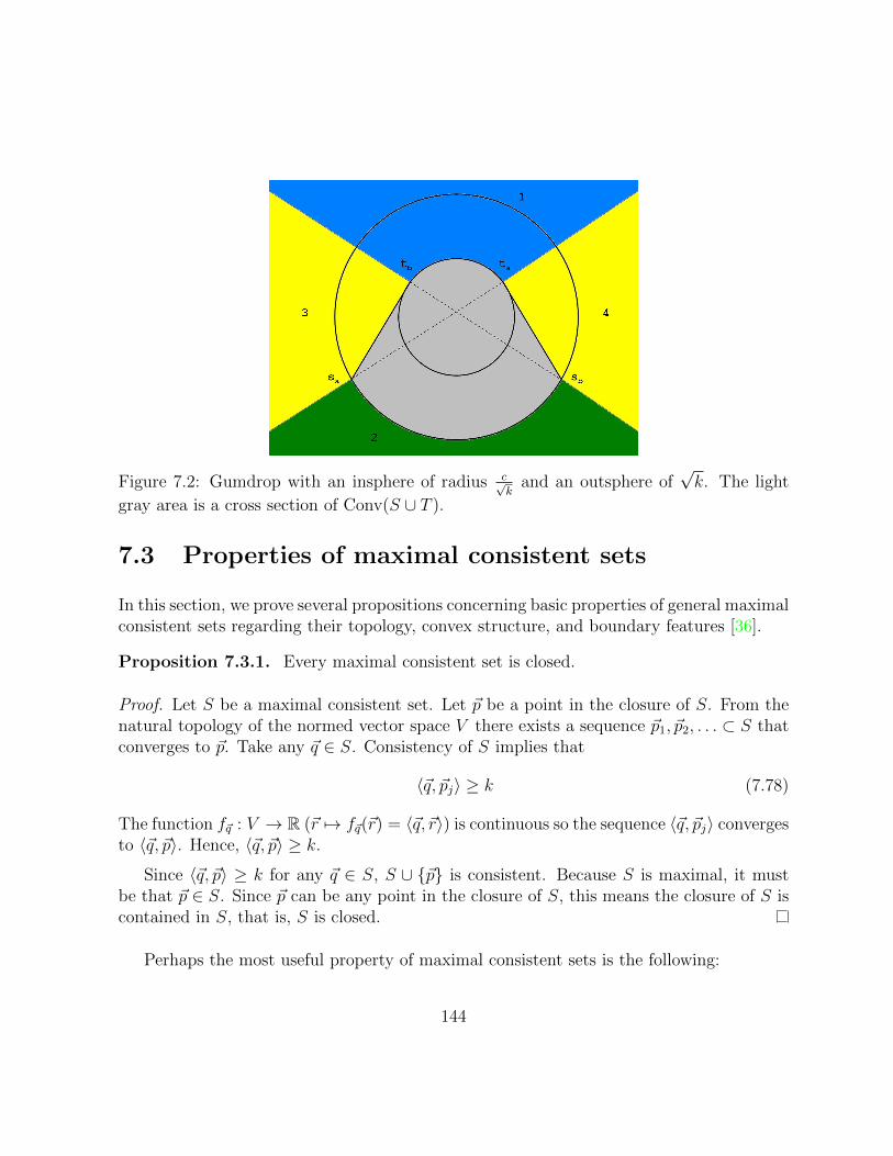
Figure 7.2: Gumdrop with an insphere of radius c√k

and an outsphere of√k. The light

gray area is a cross section of Conv(S ∪ T ).

7.3 Properties of maximal consistent sets

In this section, we prove several propositions concerning basic properties of general maximalconsistent sets regarding their topology, convex structure, and boundary features [36].

Proposition 7.3.1. Every maximal consistent set is closed.

Proof. Let S be a maximal consistent set. Let ~p be a point in the closure of S. From thenatural topology of the normed vector space V there exists a sequence ~p1, ~p2, . . . ⊂ S thatconverges to ~p. Take any ~q ∈ S. Consistency of S implies that

〈~q, ~pj〉 ≥ k (7.78)

The function f~q : V → R (~r 7→ f~q(~r) = 〈~q, ~r〉) is continuous so the sequence 〈~q, ~pj〉 convergesto 〈~q, ~p〉. Hence, 〈~q, ~p〉 ≥ k.

Since 〈~q, ~p〉 ≥ k for any ~q ∈ S, S ∪ {~p} is consistent. Because S is maximal, it mustbe that ~p ∈ S. Since ~p can be any point in the closure of S, this means the closure of S iscontained in S, that is, S is closed.

Perhaps the most useful property of maximal consistent sets is the following:

144

Proposition 7.3.2. Every maximal consistent set is convex.

Proof. First we show that if R is consistent, then the convex hull Conv(R) of R is alsoconsistent. Suppose ~p, ~q ∈ Conv(R). Then there exists ~x1, . . . , ~xM ∈ R and ~y1, . . . , ~yM ∈ Rsuch that

~p =∑i

αi~xi, ~q =∑j

βj~yj (7.79)

where∑

j αi = 1 =∑

j βj with αi, βj ≥ 0, that is, we can write ~p and ~q as a convexcombination of elements in R. Because ~xi and ~yj are elements of R, they are consistent,i.e.,

〈~xi, ~yj〉 ≥ k. (7.80)

Since αi, βj ≥ 0, it follows that αiβj 〈~xi, ~yj〉 ≥ αiβjk. Thus,

〈~p, ~q〉 =∑i,j

αiβj 〈~xi, ~yj〉 ≥∑i,j

αiβjk = k (7.81)

so ~p and ~q are also consistent. The convexity of maximal consistent sets follows from thefact that given S is maximal, for any consistent subset R ⊆ S, then Conv(R) ⊆ S. Inparticular, if R = S then Conv(S) = S.

An example of a maximal consistent set that is unbounded would be the positive quad-rant Q++ in R2 since

∀~p, ~q ∈ Q++, 〈~p, ~q〉 ≥ 0. (7.82)

Typically, we are interested only in bounded consistent sets since physically interesting setssuch as classical and quantum state spaces are examples of bounded maximal consistentsets. It turns out that a simple condition is sufficient to guarantee that a consistent set isbounded:

Proposition 7.3.3. Let R be a consistent set. If R contains the ball B = {~p ∈ V | ‖~p‖ ≤C,C > 0}, then R is contained in the ball B′ =

{~p ∈ V |‖~p‖ ≤ k

C

}.

Proof. First, observe that if R contains a ball, R must contain a pair of points whose innerproduct is negative. Therefore, k is negative.

Suppose ~q ∈ V with 〈~q, ~q〉 >(kC

)2. If we write ‖~q‖ =

√〈q, q〉 then

~q′ = − C

‖~q‖~q, (7.83)

145

which is an element of R since

〈~q′, ~q′〉 =C2

〈~q, ~q〉〈~q, ~q〉 = C2 (7.84)

meaning it lies on the ball B contained in R. Because

〈~q, ~q′〉 = − C

‖~q‖〈~q, ~q〉 < − Ck2

‖~q‖C2= − k2

C‖~q‖< k, (7.85)

any set that contains both ~q and ~q′ is inconsistent. Since ~q′ ∈ R, ~q 6∈ R for any ~q ∈ V .Thus, R can not include any point ~q with ‖~q‖ > k

C.

Proposition 7.3.4. Let S be a maximal consistent set. If S is contained in the ball{~p ∈ V | ‖~p‖ = C} for C > 0 then the ball

{~p ∈ V | ‖~p‖ = k

C

}is contained in S.

Proof. Let p be a point with 〈~p, ~p〉 =(kC

)2. Take any ~q ∈ S. By assumption 〈~q, ~q〉 < C2.

From the Cauchy-Schwarz inequality, we are guaranteed that

| 〈~p, ~q〉 |2 ≤ 〈~p, ~p〉 〈~q, ~q〉 =k2

C2(C2) = k2 (7.86)

Because k < 0, 〈~p, ~q〉 ≥ k for any ~q ∈ S. Thus, S ∪ {~p} is a consistent set. However, S ismaximal so ~p ∈ S. The only condition we imposed on ~p is 〈~p, ~p〉 = k2

C2 so it follows that

{~p ∈ V | 〈~p, ~p〉 = k2

C2} is included in S.

Proposition 7.3.5. Every maximal consistent set that includes any open neighborhoodof the origin is bounded and compact.

Proof. Proposition 7.3.3 tells us that a consistent set which includes a ball around the originis necessarily bounded. Proposition 7.3.4 suggests that a bounded maximal consistentset includes some finite ball around the origin. That takes care of the bounded part.Compactness follows from the fact that a maximal consistent set is closed and bounded inEuclidean space.

The following proposition states that there is a minimum size to any maximal consistentset:

Proposition 7.3.6. No maximal consistent set can fit inside the ball{~p ∈ V | ‖~p‖ = C <

√|k|}. (7.87)

146

Proof. Assume that S is a maximal consistent set contained in {~p ∈ V | ‖~p‖ <√|k|}. By

Proposition 7.3.1, S is closed soB = max

~p∈S〈~p, ~p〉 (7.88)

is well-defined and S is contained in {~p ∈ V | 〈~p, ~p〉 = B}. It follows from our assumptionthat B < |k|. By Proposition 7.3.4, {~p ∈ V | 〈~p, ~p〉 = k2

C2} ⊂ S. But C2 < |k| implies thatk2

C2 > |k| > B, which is a contradiction. Thus, S can not be contained within the ball ofradius C.

The next few results concern boundary properties of maximal consistent sets.

Lemma 7.3.1. Let S be bounded maximal consistent set and ~p ∈ V . If 〈~p, ~q〉 > k for all~q ∈ S then there exists ε > 0 such that 〈~p, ~q〉 ≥ k + ε.

Proof. The function f~p : S → R (~q 7→ 〈~p, ~q〉) is a continuous function with a compactdomain. Therefore, f~p has a minimum value. If f~p(~q) > k for all ~q ∈ S then min f~p(~q) ≥ k+εfor all ~q ∈ S then we can always choose

ε =min f~p − k

2. (7.89)

Lemma 7.3.2. Let S be a bounded maximal consistent set and let ~p ∈ S. If there existsε > 0 such that 〈~p, ~q〉 ≥ k + ε for all ~q ∈ S then ~p is not in the boundary of S.

Proof. Suppose there is some ε > 0 such that 〈~p, ~q〉 ≥ k + ε for all ~q ∈ S. Then

〈~p+ ~v, ~q〉 ≥ k + ε+ 〈~v, ~q〉 (7.90)

for all ~q ∈ S and ~v ∈ V . Because S is bounded there exists M > 0 such that 〈~q, ~q〉 ≥M2.By the Cauchy-Schwarz inequality

| 〈~v, ~q〉 |2 ≤ 〈~v,~v〉 〈~q, ~q〉 = ε2 (7.91)

for ~v ∈ V such that 〈~v,~v〉 =(εM

)2. Thus 〈~p+ ~v, ~q〉 ≥ k for all ~v with 〈~v,~v〉 =

(εM

)2. Hence

S contains an open ball of radius εM

centered on ~p. Therefore, ~p is not on the boundary ofS.

Proposition 7.3.7. Let S be a maximal consistent set and ~p ∈ S. The point ~p is on theboundary of S if and only if there exists ~q ∈ S such that 〈~p, ~q〉 = k.

147

Proof. Suppose ~p is on the boundary of S. By Lemma 7.3.2, there is no ε > 0 such that〈~p, ~q〉 ≥ k+ ε. By Lemma 7.3.1, 〈~p, ~q〉 > k does not hold for all ~q ∈ S. However, since S isconsistent, it must be that 〈~p, ~q〉 ≤ k. Therefore, there exists ~q ∈ S such that 〈~p, ~q〉 = k.

Now suppose there is ~q ∈ S such that 〈~p, ~q〉 = k. Any open neighborhood of ~p contains(1 + δ)~p for some δ > 0. Thus 〈(1 + δ)~p, ~q〉 = (1 + δ)k < k since k < 0. So (1 + δ)~p 6∈ S.Hence, every open neighborhood of ~p contains a point outside of S. Since every openneighborhood of ~p also contains a point in ~p, namely ~p itself, then ~p is on the boundary ofS.

Corollary 7.3.3. Let S be a maximal consistent set and ~p, ~q ∈ S. If 〈~p, ~q〉 = k then ~p, ~qare on the boundary of S.

Proposition 7.3.8. Let S be a maximal consistent set and ~p ∈ S. If ‖~p‖ = max~q∈S ‖~q‖then both ~p and k

‖~p‖2 ~p are on the boundary of S.

Proof. By Proposition 7.3.4, S contains the ball{~q ∈ V | ‖~q‖ < k

||p||

}Therefore, k

‖~p‖2 ~p ∈ S.

Since⟨

k‖~p‖2 ~p, ~p

⟩= k, Corollary 1 implies that ~p and k

‖~p‖2 ~p are on the boundary of S.

The next propositions indicate that a suitably placed origin for a consistent set deter-mines the value for ‖~p‖ for ~p ∈ S:

Proposition 7.3.9. Let R be a consistent set with 〈~p, ~q〉 ≥ k, k < 0. If for some ~p, ~q ∈ R

the origin O = α~p+ (1− α)~q for α ∈ [0, 12) then ~p, ~q ∈

{~r ∈ V | ‖~r‖ ≤

√|k|(1−α)

α

}.

Proof. For the origin, ‖O‖2 = 0 so

0 = 〈α~p+ (1− α)~q, α~p+ (1− α)~q〉= α2‖~p‖2 + 2α(1− α) 〈~p, ~q〉+ (1− α)2‖~q‖2 (7.92)

which means thatα2‖~p‖2 + (1− α)2‖~q‖2 ≤ −2α(1− α) 〈~p, ~q〉 . (7.93)

But 〈~p, ~q〉 ≥ k =⇒ −〈~p, ~q〉 ≤ 2|k| so

α2‖~p‖2 + (1− α)2‖~q‖2 ≤ 2|k|α(1− α). (7.94)

148

Let 0 ≤ α < 12. Since α~p = −(1− α)~q, we can write

‖~p‖ =

∣∣∣∣1− αα∣∣∣∣ ‖~q‖ (7.95)

and so we get

‖~q‖2 ≤ |k|α(1− α)

and ‖~p‖2 ≤ |k|(1− α)

α. (7.96)

Proposition 7.3.10. Let S be a consistent set with 〈~p, ~q〉 ≥ k for all ~p, ~q ∈ S.If

{~pi}+N+1i=1 ⊂ S (7.97)

with 〈~pi, ~pj〉 = C when i 6= j, for k ≤ C < 0 and∑N+1

i=1 ~pi = 0, then ‖~pi‖ =√N |C|.

Proof. For any j 6= k, 〈~pj, ~pk〉 = C. Note that

− ~pj =N+1∑i=1,i 6=j

~pi. (7.98)

Thus,

〈~pj, ~pk〉 = −N+1∑i=1,i 6=j

〈~pi, ~pk〉

= −〈~pk, ~pk〉 −N+1∑

i=1,i 6=j,i6=k

〈~pi, ~pk〉 (7.99)

implies that‖~pk‖2 = −C − (N + 1− 2)C = N |C|. (7.100)

7.4 Maximization of consistent sets: examples

We want to consider the following problem. Suppose we are given some consistent setR ⊂ V with consistency given by 〈p, q〉 > k, for any p, q ∈ R. We want to add all points

149

vi ∈ V such that 〈r, q〉 ≥ k for all points in S ∪ {v1, v2, . . .}, that is, we add all points inV such that S is a maximal consistent set. We denote this process by S = Max(R). Isit then possible to characterize the types of maximal consistent sets you can obtain fromconsistent sets with a finite number of points? For instance, are there cases where theconsistent set leads to a unique maximization? Here we want describe a few examplesshowing that this is indeed the case, which opens the possibility that quantum state spaceitself is a maximization of a suitably chosen initial consistent set. If we can find thesimplest consistent set then it means that the essential geometric aspects of the set ofquantum states is embodied by the symmetries possessed by the initial consistent set. Butbefore we get to that, it is useful to have a better understanding of what it means tomaximize a consistent set, which is, in fact, a highly nontrivial task.

The first example we consider is a consistent set with two vectors whose inner productdefines the consistency condition. It demonstrates that, for identifying the maximization,it is often crucial to wisely choose the origin and the orientation of coordinates.

Example 7.4.1. Let V = R2 and R = {~a,~b} is a consistent set with

~a =

(a1

a2

)and ~b =

(b1

b2

), (7.101)

and consistency is given by k =⟨~a,~b⟩

. The midpoint of ~a and ~b is given by

~m =

(a1+b1

2a2+b2

2

). (7.102)

Performing the translation ~x 7→ ~x′ = ~x− ~m so that

~m 7→ ~m′ =

(0

0

), ~a 7→ ~a′ =

(b1−a1

2b2−a2

2

), ~b 7→ ~b′ =

(a1−b1

2a2−b2

2

), (7.103)

we get the translated consistent setR′ with consistency given by k′ =⟨~a′,~b′

⟩. Furthermore,

we can rotate coordinates using

O =

(cos θ sin θ

− sin θ cos θ

)where tan θ =

a′2a′1

=b2 − a2

b1 − a1

. (7.104)

150

Note that the minus sign for the rotation matrix is on the second row since we are per-forming a passive transformation. After the rotation, we obtain the consistent set R′′ withelements

O~m′ = ~m′,

~a′′ = O~a′ =

(s

0

), (7.105)

~b′′ = O~b′ =

(−s0

),

where

s =√〈~a′,~a′〉 =

√⟨~b′,~b′

⟩=

1

4

[(x1 − x2)2 + (y1 − y2)2] . (7.106)

Hence, the consistency condition for Max (R′′) is given by

− s2 ≤ 〈~p′′, ~q′′〉 ≤ s2, ∀~p′′, ~q′′ ∈ Max (R′′) . (7.107)

The upper bound just follows from the fact that ~a′′ and ~b′′ are equidistant from the originand maximally distant from each other.

Suppose

~p′′ =

(s cosα

s sinα

), and ~q′′ =

(s cos β

s sin β

). (7.108)

Then we have

〈~p′′, ~q′′〉 = s2 cosα cos β + s2 sinα sin β (7.109)

= s2 cos(α− β).

Since −1 ≤ cos(α− β) ≤ 1 ∀α, β ∈ R

− s2 ≤ 〈~p′′, ~q′′〉 ≤ s2 (7.110)

for all such ~p′′, ~q′′. This means that the set of points

T ={

(~x, ~y)| ~x2 + ~y2 = s2}

(7.111)

is consistent with R′′. Moreover, any such point ~p has 〈~p, ~p〉 = s2, so it must lie on theboundary of Max (R′′).

151

Since T is consistent, Conv(T ) is consistent. Thus,

Conv(T ) ⊆ Max (R′′) . (7.112)

To show that they are in fact equal, consider any point ~r lying outside Conv(T ). If youfind the point ~t on T that is closest to ~r, it is easy to show that the point opposite to thaton the circle will be inconsistent with ~r, i.e.

⟨~r,−~t

⟩< −s2.

Of course, to get Max(R), just undo the rotation and translation on Max (R′′). Thegeneralization for a pair of points from Rd is that the maximal consistent set is a ball wherethe two points lie on the surface.

Next we consider the vertices of a regular simplex. If the consistency condition is chosenappropriately, the simplex itself can be considered as a maximal consistent set.

Example 7.4.2. Suppose we have for pairwise maximally distant probability vectors~p1, ~p2, ~p3, ~p4 from the 3-simplex. Without loss of generality, these probability vectors canbe specified with coordinates

~p1 =

a

b

c

d

, ~p2 =

b

c

d

a

, ~p3 =

c

d

a

b

, ~p4 =

d

a

b

c

, (7.113)

and since these must be probabilities,

a+ b+ c+ d = 1 (7.114)

for a, b, c, d ≥ 0, and with the added constraint

(ab+ bc+ cd+ da) = 2(ac+ bd) (7.115)

to ensure that pairwise inner products are equal. Using these coordinates, consistency isgiven by

〈~p, ~q〉 ≥ ab+ bc+ cd+ da. (7.116)

Performing the same manipulations as before, we translate the origin to

~m =

14141414

, (7.117)

152

which would be equivalent to the translation ~pi 7→ ~qi = ~pi − ~m for i = 1, 2, 3, 4. If wedenote the squared norm of ~qj by N = 〈~qj, ~qj〉 for any j, it is easy to verify that

〈~qi, ~qj〉 = −N3

(7.118)

for any distinct pair i, j = 1, 2, 3, 4. Now consider the matrix

Q =

〈q1, q1〉 〈q1, q2〉 〈q1, q3〉 〈q1, q4〉〈q2, q1〉 〈q2, q2〉 〈q2, q3〉 〈q2, q4〉〈q3, q1〉 〈q3, q2〉 〈q3, q3〉 〈q3, q4〉〈q4, q1〉 〈q4, q2〉 〈q4, q3〉 〈q4, q4〉

=N

3

3 −1 −1 −1

−1 3 −1 −1

−1 −1 3 −1

−1 −1 −1 3

. (7.119)

The matrix Q has exactly 1 zero eigenvalue corresponding to eigenvector (1, 1, 1, 1)T . Notethat the linear dependency condition ∑

j

aj~qj = 0 (7.120)

holds if and only if the vector

~a =

a1

a2

a3

a4

(7.121)

is a zero eigenvector of Q. Therefore, the space spanned by {~q1, ~q2, ~q3, ~q4} is exactly 3-dimensional. Coupled with the fact that the angles between any pair of vectors ~qi arethe same, these vectors point to vertices of a regular tetrahedron. To see this, it may beconvenient to rotate the coordinates of ~qj such that

~q1 =√N

0

0

1

0

, ~q2 =

√N

3

√

8

0

−1

0

, ~q3 =

√N

3

−√

2√

6

−1

0

, ~q4 =

√N

3

−√

2

−√

6

−1

0

.

(7.122)From here, it is straightforward to show that on the sphere S given by

x21 + x2

2 + x23 = N, x4 = 0. (7.123)

153

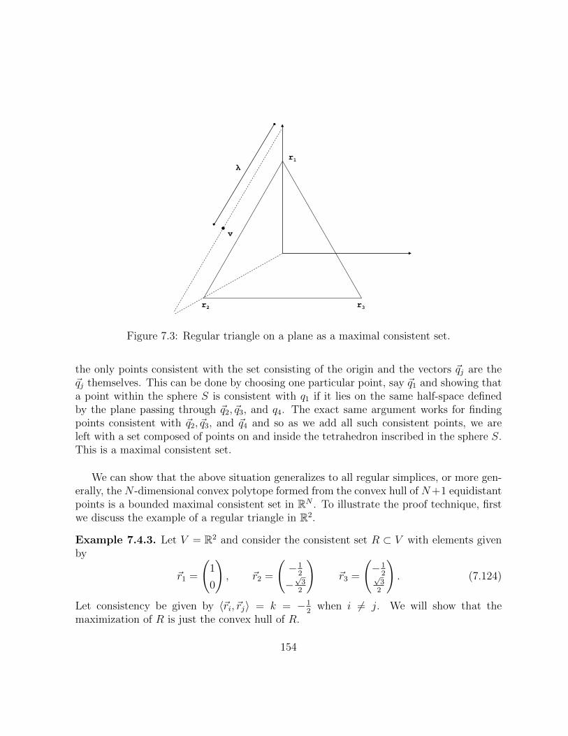
r1

r2 r3

v

λ

Figure 7.3: Regular triangle on a plane as a maximal consistent set.

the only points consistent with the set consisting of the origin and the vectors ~qj are the~qj themselves. This can be done by choosing one particular point, say ~q1 and showing thata point within the sphere S is consistent with q1 if it lies on the same half-space definedby the plane passing through ~q2, ~q3, and q4. The exact same argument works for findingpoints consistent with ~q2, ~q3, and ~q4 and so as we add all such consistent points, we areleft with a set composed of points on and inside the tetrahedron inscribed in the sphere S.This is a maximal consistent set.

We can show that the above situation generalizes to all regular simplices, or more gen-erally, the N -dimensional convex polytope formed from the convex hull of N+1 equidistantpoints is a bounded maximal consistent set in RN . To illustrate the proof technique, firstwe discuss the example of a regular triangle in R2.

Example 7.4.3. Let V = R2 and consider the consistent set R ⊂ V with elements givenby

~r1 =

(1

0

), ~r2 =

(−1

2

−√

32

)~r3 =

(−1

2√3

2

). (7.124)

Let consistency be given by 〈~ri, ~rj〉 = k = −12

when i 6= j. We will show that themaximization of R is just the convex hull of R.

154

Proof. Consistency of Conv(R) follows naturally from the consistency of R. To showmaximality, suppose we consider some ~v ∈ V where ~v is not inside the convex hull of R.For any such ~v, we can write

v = λα~pi + (1− λ)β~pj (7.125)

where i, j = 1, 2, 3, i 6= j, α, β ≥ 1, and 0 ≤ λ ≤ 1. For example, for the particular ~vdepicted in Fig. 7.3, it can be written as the convex combination of rescaled vectors ~r1 and~r2.

Thus, upon maximizing R, we require that

〈~v, ~pk〉 = λα 〈~pi, ~pk〉+ (1− λ)β 〈~pj, ~pk〉 ≥ k (7.126)

for all k = 1, 2, 3. However, when i 6= j 6= k, we get

〈~v, ~pk〉 = [λα + (1− λ)β] k ≤ k (7.127)

since k < 0 and λα+(1−λ)β ≥ 1, with equality if and only if α = β = 1. However, if thatholds, then it would mean that ~v ∈ Conv(R), which is a contradiction. Therefore, if ~v ∈ Vis not in the convex hull of R, it will be inconsistent with one of the elements of R.

It is not hard to see how procedure generalizes to higher dimensions:

Theorem 7.4.1. Let R ⊂ V be the consistent set

R =

{~r1, ~r2, . . . , ~rN+1 |

N+1∑i=1

ri = 0

}, (7.128)

where consistency is given by〈~ri, ~rj〉 = k for all i 6= j and V = Span(R). Then Conv(R) isthe maximal consistent set Max(R) obtained from maximizing R.

Proof. Consistency follows trivially from the consistency of R. Maximality can be shownby contradiction as follows: suppose ~v ∈ V and ~v 6∈ Conv(R). Because R spans V , thereexists sets of N numbers {λi}Ni=1 and {αi}Ni=1 such that

~v =∑i 6=j

λi (αi~ri) (7.129)

where0 ≤ λi ≤ 1,

∑i 6=j

λi = 1 (7.130)

155

and αi ≥ 1. This merely tells us that can write ~v as a convex combination of N stretchedvectors in R. Maximizing R by adding all such consistent ~v, we have

〈~v, ~rk〉 =∑i 6=j

λi 〈αi~ri, ~rk〉 ≥ k. (7.131)

for all k = 1, 2, ..., N + 1. However, we note that in the case k = j, we obtain

〈~v, ~rj〉 =∑i 6=j

λi 〈αi~ri, ~rj〉 =

[∑i 6=j

λiαi

]k ≤ k (7.132)

with equality if and only if αi = 1 for all i. But that happens only when ~v ∈ Conv(R),which contradicts our initial assumption on ~v. Therefore, ~v ∈ V is included in Max(R) ifand only if it is in the convex hull of R.

The important lesson to take away from the examples of this section is that for consis-tent sets with the appropriate consistency condition, there corresponds a unique maximalconsistent set. This suggests the possibility of constructing quantum state space from themaximization of a suitable consistent set.

7.5 Qutrit state space as a maximal consistent set

In this section, we sketch some of the details for constructing quantum state space in d = 3as the maximization of some initial consistent set. As a matter of convenience, we adoptthe bracket notation, where |p〉 and |q〉 represent two vectors in Rd2 and the bracket 〈p|q〉is just the dot product between the two real vectors. For qutrits, consistency between SICprobability vectors given by

1

12≤ 〈p|q〉 ≤ 1

6. (7.133)

Let {|j〉}d2j=1 form the standard basis in Rd2 . To start, we consider the consistent set

S0 ⊂ ∆d2−1 of probability vectors,

S0 = {|Ek〉 , |Zijk〉 | i, j, k = 1, 2, . . . , 9 for i 6= j 6= k} , (7.134)

where the |Ek〉 are called the basis distributions

|Ek〉 =9∑j=1

3δjk + 1

12|j〉 =

1

12(1, ...,

kth︷︸︸︷4 , ...1), (7.135)

156

which are just the probability vectors generated from the SIC elements by the SIC repre-sentation, and the |Zrst〉 are uniform maximal-zero distributions

|Zrst〉 =9∑j=1

1

9− β(1− δrj − δsj − δtj) |j〉 , for r 6= s 6= t (7.136)

where β is the maximum number of zero-valued components allowed, which happens toβ = 3 in this case. Writing |Zrst〉 out explicitly gives

|Zrst〉 =1

6(1, ..,

rth︷︸︸︷0 , . . . ,

sth︷︸︸︷0 , . . . ,

tth︷︸︸︷0 , . . . , 1) (7.137)

What we want is a recipe for building up a maximal consistent set from S0.

First, we add all the probability vectors |Qrst〉 such that is maximally distant with both

|Er〉 and |Zrst〉:〈Er|Qr

st〉 = 〈Zrst|Qrst〉 =

1

12. (7.138)

This is possible because if we consider the corresponding vectors in Hilbert space, this justsays that for every pair of orthogonal pure states, there is another pure state such that thethree unit vectors form an orthonormal basis.

For example, if we take |E1〉 and |Z123〉 then it turns out that there is only one choicefor a third point |Q1

23〉, which is∣∣Q123

⟩=

1

12(0, 3, 3, 1, 1, 1, 1, 1, 1) (7.139)

where our notation is meant to suggest that it is maximally distant to the probabilityvectors |E1〉 and |Z123〉. We say that |E1〉, |Z123〉 and |Q1

23〉 form a maximally distanttriplet.In geometric terms, |Q1

23〉 is the third point along with |Z123〉 and |E1〉 that forms

an equilateral triangle inscribed in the out-sphere of radius√

2d(d+1)

= 1√6

and there can

only be one such point.

We want to include all such probability vectors for all possible maximally distant pairs|Er〉 and |Zrst〉. We find that the vectors |Qr

st〉 come with a generic form: its rth entry iszero, the sth and tth entries are both 1

4and all remaining entries are 1

12.

However, in order to maintain consistency in the new set S1 = S0 ∪ {|Qrst〉}, the |Zrst〉

that are inconsistent with the |Q〉rst have to be excluded. For instance, in the example with|E1〉 , |Z123〉 , and |Q1

23〉, we observe that

〈Q123|Z23k〉 =

5

72<

1

12, k = 4, 5, ..., 9 (7.140)

157

so the price for including |Q123〉 to S while retaining consistency is to remove 6 uniform

maximal-zero distributions from the set.

If we keep on adding as many |Qrst〉 as we can, how many |Zrst〉 remain in the new set

S1? There are a number of different ways to get at the answer but by a simple countingargument, we can see that we will be left with 12 pairs before all |Zrst〉 are exhausted. Aswe saw in the example above, adding |Qr

st〉 requires removing six points |Zkst〉 , k 6= r, s, t,it follows that since there are

9C3 =

(9

3

)= 84 (7.141)

uniform maximal-zero distributions |Zrst〉 and each step of adding |Qrst〉 involves 7 such

vectors, only one of which is kept in the new set, then we can add up to 84÷ 7 = 12 |Qrst〉before we end up considering all |Zrst〉. The actual 12 that are left the order in which weconsider pairs |Er〉 and |Zrst〉 but whichever set we end up with will be related to anotherpossible set by a permutation of indices.

It is always possible to perform the procedure such that the 12 maximal-zero distribu-tions that remain are

|Z123〉 , |Z456〉 , |Z789〉 , |Z147〉 , |Z258〉 , |Z369〉 , |Z159〉 , |Z267〉 , |Z348〉 , |Z168〉 , |Z249〉 , |Z357〉 ,(7.142)

that is, |Zrst〉 with index triples (rst) that correspond to the affine lines in1 2 3

4 5 6

7 8 9

, (7.143)

which is just the sort of finite affine-plane structure we have encountered before.

So each pair |Er〉 , |Zrst〉 allows us to add |Qrst〉. Certainly, we could have instead

considered |Es〉 , |Zrst〉 which would tell us to add |Qstr〉. For example,

〈E1|Q231〉 =

[1

12(4, 1, 1, 1, 1, 1, 1, 1, 1)

]·[

1

12(3, 0, 3, 1, 1, 1, 1, 1, 1)

](7.144)

=1

144(12 + 3 + 6) =

21

144=

7

48>

1

12.

We may also consider pairs |E〉q and |Z〉rst that do not share any indices. As an example,

〈E5|Q231〉 =

[1

12(1, 1, 1, 1, 3, 1, 1, 1, 1)

]·[

1

12(3, 0, 3, 1, 1, 1, 1, 1, 1)

](7.145)

=1

144(3 + 3 + 3 + 5) =

14

144=

7

72>

1

12.

158

It is not difficult to see that in general

〈Er|Qrst〉 =

1

12, 〈Es|Qr

st〉 =7

48, 〈Eq|Qr

st〉 =7

72for distinct q, r, s, t = 1, 2, ..., 9.

(7.146)and 1

12< 7

72< 7

48< 1

6so we can add all such |Qr

st〉 and the new set remains consistent. Ifwe do so, the consistent set we end up with is

S ′ = {|Er〉 , |Zrst〉 , |Qrst〉 | r, s, t = 1, 2, ..., 9} (7.147)

where if we count elements we have 9 basis distributions, 12 uniform maximal-zero distri-butions, and 36 |Qr

st〉.

To see all the maximal-distance relations, consider |E1〉. From the 12 maximal-zerovectors in Eq. (7.142), 4 of them are maximally distant to it: |Z123〉 , |Z147〉 , |Z159〉 , and|Z168〉. To each one there is a unique |Q1

st〉 that is maximally distant to both |E1〉 and|Z1st〉. Since each basis distribution generates 4 |Qr

st〉, there must be 36 in total.

Because 〈Eq|Qrst〉 > 1

12for q 6= r, the set S ′ is actually exhaustive with regard to

forming maximally distant triplets, that is, for any pair of vectors in S ′ that are maximallydistant from each other, the third vector forming a maximally distant triplet with the pairis already in S ′.

Before going further, we ask, how do the elements of S ′ map back to unit vectors inHilbert space? This is definitely not unique since the basis distributions may correspondto any SIC in d = 3. However, if we express everything in terms of the most exceptionalSIC given by the fiducial

|ψ0〉 =

0

1

−1

(7.148)

then we observe that

(i) the basis distributions |Er〉 are the vectors corresponding to SIC projectors,

(ii) the uniform maximal-zero distributions |Zrst〉 are the set of vectors associated witha complete set of mutually unbiased bases (MUBs) in d = 3. In fact, if we consider

159

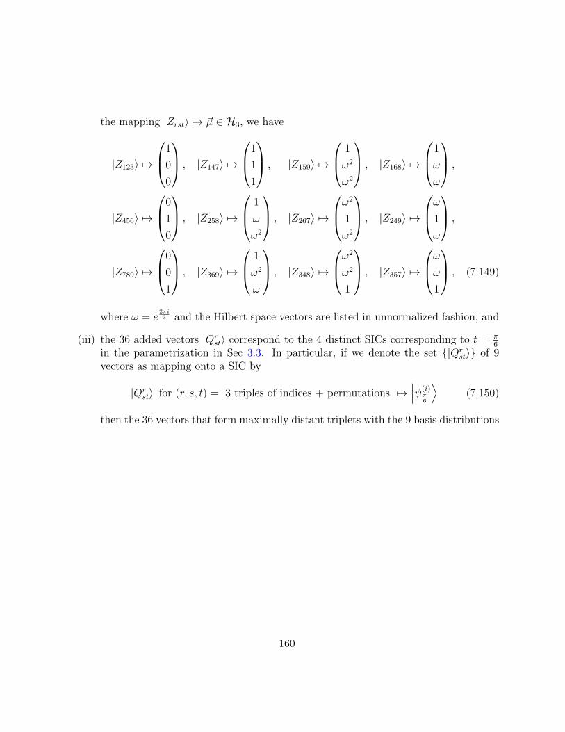
the mapping |Zrst〉 7→ ~µ ∈ H3, we have

|Z123〉 7→

1

0

0

, |Z147〉 7→

1

1

1

, |Z159〉 7→

1

ω2

ω2

, |Z168〉 7→

1

ω

ω

,

|Z456〉 7→

0

1

0

, |Z258〉 7→

1

ω

ω2

, |Z267〉 7→

ω2

1

ω2

, |Z249〉 7→

ω1ω

,

|Z789〉 7→

0

0

1

, |Z369〉 7→

1

ω2

ω

, |Z348〉 7→

ω2

ω2

1

, |Z357〉 7→

ωω1

, (7.149)

where ω = e2πi3 and the Hilbert space vectors are listed in unnormalized fashion, and

(iii) the 36 added vectors |Qrst〉 correspond to the 4 distinct SICs corresponding to t = π

6

in the parametrization in Sec 3.3. In particular, if we denote the set {|Qrst〉} of 9

vectors as mapping onto a SIC by

|Qrst〉 for (r, s, t) = 3 triples of indices + permutations 7→

∣∣∣ψ(i)π6

⟩(7.150)

then the 36 vectors that form maximally distant triplets with the 9 basis distributions

160

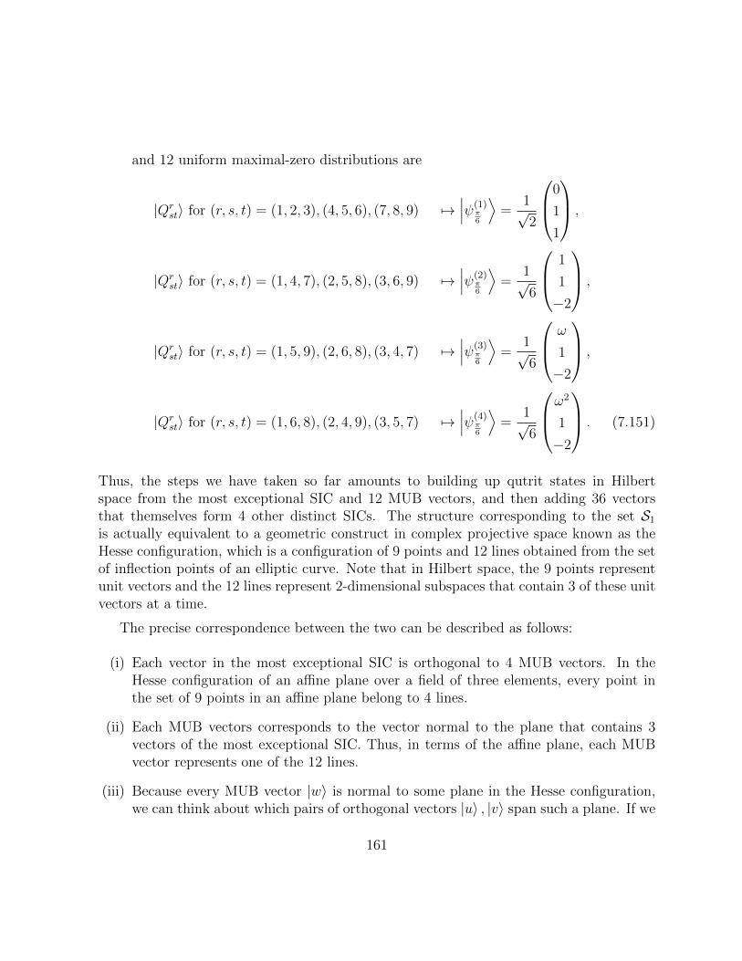
and 12 uniform maximal-zero distributions are

|Qrst〉 for (r, s, t) = (1, 2, 3), (4, 5, 6), (7, 8, 9) 7→

∣∣∣ψ(1)π6

⟩=

1√2

0

1

1

,

|Qrst〉 for (r, s, t) = (1, 4, 7), (2, 5, 8), (3, 6, 9) 7→

∣∣∣ψ(2)π6

⟩=

1√6

1

1

−2

,

|Qrst〉 for (r, s, t) = (1, 5, 9), (2, 6, 8), (3, 4, 7) 7→

∣∣∣ψ(3)π6

⟩=

1√6

ω

1

−2

,

|Qrst〉 for (r, s, t) = (1, 6, 8), (2, 4, 9), (3, 5, 7) 7→

∣∣∣ψ(4)π6

⟩=

1√6

ω2

1

−2

. (7.151)

Thus, the steps we have taken so far amounts to building up qutrit states in Hilbertspace from the most exceptional SIC and 12 MUB vectors, and then adding 36 vectorsthat themselves form 4 other distinct SICs. The structure corresponding to the set S1

is actually equivalent to a geometric construct in complex projective space known as theHesse configuration, which is a configuration of 9 points and 12 lines obtained from the setof inflection points of an elliptic curve. Note that in Hilbert space, the 9 points representunit vectors and the 12 lines represent 2-dimensional subspaces that contain 3 of these unitvectors at a time.

The precise correspondence between the two can be described as follows:

(i) Each vector in the most exceptional SIC is orthogonal to 4 MUB vectors. In theHesse configuration of an affine plane over a field of three elements, every point inthe set of 9 points in an affine plane belong to 4 lines.

(ii) Each MUB vectors corresponds to the vector normal to the plane that contains 3vectors of the most exceptional SIC. Thus, in terms of the affine plane, each MUBvector represents one of the 12 lines.

(iii) Because every MUB vector |w〉 is normal to some plane in the Hesse configuration,we can think about which pairs of orthogonal vectors |u〉 , |v〉 span such a plane. If we

161

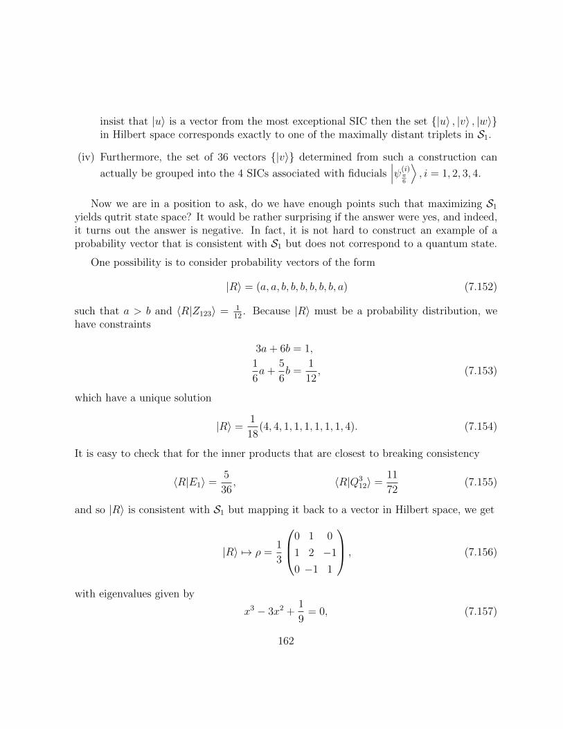
insist that |u〉 is a vector from the most exceptional SIC then the set {|u〉 , |v〉 , |w〉}in Hilbert space corresponds exactly to one of the maximally distant triplets in S1.

(iv) Furthermore, the set of 36 vectors {|v〉} determined from such a construction can

actually be grouped into the 4 SICs associated with fiducials∣∣∣ψ(i)

π6

⟩, i = 1, 2, 3, 4.

Now we are in a position to ask, do we have enough points such that maximizing S1

yields qutrit state space? It would be rather surprising if the answer were yes, and indeed,it turns out the answer is negative. In fact, it is not hard to construct an example of aprobability vector that is consistent with S1 but does not correspond to a quantum state.

One possibility is to consider probability vectors of the form

|R〉 = (a, a, b, b, b, b, b, b, a) (7.152)

such that a > b and 〈R|Z123〉 = 112

. Because |R〉 must be a probability distribution, wehave constraints

3a+ 6b = 1,

1

6a+

5

6b =

1

12, (7.153)

which have a unique solution

|R〉 =1

18(4, 4, 1, 1, 1, 1, 1, 1, 4). (7.154)

It is easy to check that for the inner products that are closest to breaking consistency

〈R|E1〉 =5

36, 〈R|Q3

12〉 =11

72(7.155)

and so |R〉 is consistent with S1 but mapping it back to a vector in Hilbert space, we get

|R〉 7→ ρ =1

3

0 1 0

1 2 −1

0 −1 1

, (7.156)

with eigenvalues given by

x3 − 3x2 +1

9= 0, (7.157)

162

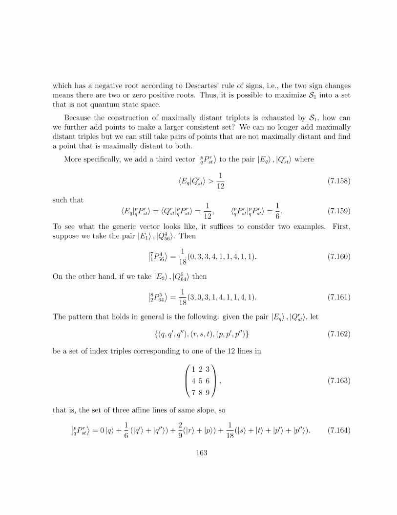
which has a negative root according to Descartes’ rule of signs, i.e., the two sign changesmeans there are two or zero positive roots. Thus, it is possible to maximize S1 into a setthat is not quantum state space.

Because the construction of maximally distant triplets is exhausted by S1, how canwe further add points to make a larger consistent set? We can no longer add maximallydistant triples but we can still take pairs of points that are not maximally distant and finda point that is maximally distant to both.

More specifically, we add a third vector∣∣pqP

rst

⟩to the pair |Eq〉 , |Qr

st〉 where

〈Eq|Qrst〉 >

1

12(7.158)

such that

〈Eq|pqP rst〉 = 〈Qr

st|pqP rst〉 =

1

12, 〈pqP r

st|pqP rst〉 =

1

6. (7.159)

To see what the generic vector looks like, it suffices to consider two examples. First,suppose we take the pair |E1〉 , |Q4

56〉. Then∣∣71P

456

⟩=

1

18(0, 3, 3, 4, 1, 1, 4, 1, 1). (7.160)

On the other hand, if we take |E2〉 , |Q564〉 then∣∣8

2P564

⟩=

1

18(3, 0, 3, 1, 4, 1, 1, 4, 1). (7.161)

The pattern that holds in general is the following: given the pair |Eq〉 , |Qrst〉, let

{(q, q′, q′′), (r, s, t), (p, p′, p′′)} (7.162)

be a set of index triples corresponding to one of the 12 lines in 1 2 3

4 5 6

7 8 9

, (7.163)

that is, the set of three affine lines of same slope, so∣∣pqP

rst

⟩= 0 |q〉+

1

6(|q′〉+ |q′′〉) +

2

9(|r〉+ |p〉) +

1

18(|s〉+ |t〉+ |p′〉+ |p′′〉). (7.164)

163

It is not as complicated as it looks because relevant 5 indices correspond exactly to 2intersecting lines in the affine plane, with the intersection point given by the raised indexr in |Qr

st〉 and the intersecting lines (p, q, r) and (r, s, t) are uniquely specified by q and s, t.

It is not difficult to check that we can add all such vectors since for the most importantinner products we get

〈Zpqr|pqP rst〉 =

5

54, 〈Qp

p′p′′ |pqP

rst〉 =

1

12. (7.165)

Note that because the second inner product corresponds to a new pair of maximally distantpoints, it is possible to add more points by constructing maximally distant triplets withsuch pairs if desired. Also, at least one of

∣∣pqP

rst

⟩will be inconsistent with probability

vectors of the form |R〉 in Eq. (7.154) so those non-quantum points are precluded from anymaximization of the consistent set S1 ∪ {

∣∣pqP

rst

⟩}.

So how many vectors∣∣pqP

rst

⟩can we add to set S1? Each

∣∣pqP

rst

⟩is determined by 5

indices, (r, s, t) corresponding to an affine line. From the index triple (r, s, t), we pick 1index, r, as the intersection point and we select 1 of the 3 other lines that pass throughr, specifically the line that passes through q. Thus, counting all possible combinations,12× 3× 3 = 108.

Hence, after adding all possible∣∣pqP

rst

⟩we have

S2 ={|Eq〉 , |Zrst〉 , |Qr

st〉 ,∣∣pqP

rst

⟩| all distinct q, r, s, t = 1, 2, ..., 9

}. (7.166)

so the cardinality of the new consistent set is |S2| = 108 + 57 = 165.

So how far is Max(S2) from quantum state space? Unfortunately, right now, all we cansay is that quantum state space is one of its possible maximizations. It turns out thatthe discussion in Sec. 7.6 will show that a lot more structure is needed to pick out thequantum case uniquely.

As it stands, the two most promising possibilities for getting quantum state space fromS2 is the following:

(i) The way we add more points to enlarged the set must involve some additional sym-metry requirement. It might be possible to indirectly impose the symmetry by aidentifying special points in the boundary of quantum state space that are not ex-treme points as having some geometrical significance. The problem with adding suchpoints is that in the way we have been enlarging the consistent set, it seems veryunnatural to add points that do not correspond to pure states.

164

(ii) The other possibility is to continue adding a maximally distant point to all pairs inS2 that is consistent with all points already in the set. The added points will thenintroduce new pairings to the set and we can proceed with the process. We do notknow if the process continues indefinitely but if it does, the conjecture is that Snconverges to a set that densely covers the set of all pure states.

7.6 Duality and symmetry of maximal consistent sets

To make further progress in our attempts to build up quantum state space from a finiteconsistent set, we need more mathematical tools to see how far maximal consistency cantake us. To this end, we introduce the concept of a dual set for consistent sets and examineits implications for the symmetry of the maximization of consistent sets.

Consider any finite-dimensional normed vector space V and C > 0. For some subsetS ⊂ V , we can define the dual set

S = Dual(S) = {~v ∈ V | 〈~v, ~w〉 ≥ −C ∀~v ∈ S}. (7.167)

The value C determines the scale of dual vectors and is not crucial in most cases.

Denoting the dual set of S by S = Dual(S), some of the basic properties of dual setsare

(i) The dual set is closed and convex.

(ii) The dual of the dual set Dual(S) is the convex hull of S if S contains the origin.

(iii) The dual of the union of 2 sets S and T is the intersection of the dual set for each,i.e.,

Dual(S ∪ T ) = S ∩ T . (7.168)

(iv) The dual of the intersection of 2 closed convex sets S and T that include the originis the convex hull of the union of their dual sets, i.e.,

Dual(S ∩ T ) = Conv(S ∪ T ). (7.169)

We are interested in the dual of consistent sets. Given a consistent set S whose centroidor geometric center is at the origin, and with consistency given by

〈~p, ~q〉 = k ∀ ~p, ~q ∈ S, (7.170)

165

then for any non-zero vector ~p ∈ S we can define a dual vector ~p = Dual(~p),

~p =k

‖~p‖2~p (7.171)

so that ⟨~p, ~p⟩

=k 〈~p, ~p〉‖~p‖2

. (7.172)

Geometrically, ~p is the vector oppositely directed to ~p along a line through the origin suchthat the points corresponding to ~p and ~p are maximally distant.

For consistent sets on the probability simplex ∆d2−1 relevant to the quantum case,

k = − 1

d2(d+ 1)(7.173)

and for each such set S, there are 3 spheres of significance:

an in-sphere with radius r =

√1

d2(d2 − 1)

an out-sphere with radius R =

√d− 1

d2(d+ 1)(7.174)

a middle sphere with radius |k| =

√1

d2(d+ 1)

The out-sphere is the smallest sphere that contains Conv(S). The in-sphere is the largestsphere that is contained in any maximization of S. The in-sphere and out-sphere are dualto each other. The middle sphere is another sphere whose radius is the geometric meanof the radii of the in-sphere and the out-sphere, and it contains points whose antipodalpoints are maximally distant to each other, that is, it is a self-dual sphere.

Several properties of maximal consistent sets follow immediately from the notion ofdual sets, that is, if S is a maximal consistent set then

(i) S contains d2 basis vectors. This follows from the duality between the simplex formedby the basis distributions and the probability simplex ∆d2−1 itself;

(ii) for every extreme point in S, there exists at least one point maximally distant to it;and

166

(iii) S is self-dual and it is given by the intersection of all half-spaces obtained from itsextreme points through the lower bound for consistency.

Huangjun Zhu has proven a number of lemmas that follow from duality considerations[136] but we mention a few of them that provide some valuable insights for the quantumreconstruction effort.

Lemma 7.6.1. Suppose S is a maximal consistent set with infinitely many points on theout-sphere. Then any polytope inscribed by S can not contain the in-sphere.

Proof. Suppose we do have a polytope P ⊂ S and the in-sphere of S is contained in P .Then Dual(P ) = P ⊃ S and is contained in the out-sphere. Consequently, S must have afinite number of points in the out-sphere. In particular, it must be less than the numberof vertices of the dual polytope P to P , which contradicts the assumption that S hasinfinitely many points on the out-sphere.

Lemma 7.6.2. Let R be a consistent set and let C be the intersection of all maximalconsistent sets that include R. If R contains C then there exists a maximization of R thathas the same points on the out-sphere as R.

Proof. The crucial element in the proof is the observation that a vector ~p on the in-sphereof R lies on the boundary of the dual of R if and only if the dual vector ~p belongs to Randis found on the out-sphere or R.

Define Ro to be the set of points in R that lie on the out-sphere. Let

T = R ∪ (R ∪ Smax) (7.175)

where Smax is the maximum inscribed sphere corresponding to (any maximization of) R.T is consistent by construction and the intersection of its boundary ∇T with the in-sphereSinconsists of the dual vectors for the elements in R, i.e.,

∇T ∪ Sin ={~p | ∀ ~p ∈ R

}(7.176)

so ~p ∈ T when ~p ∈ R. Thus, any maximization of T will fulfill the lemma.

Without some additional structure, duality seems to strongly imply that the only wayto uniquely obtain a set isomorphic to quantum state space from a consistent set is to

167

actually include all the pure states. Thus, we supplement the general properties of maxi-mal consistent sets and their dual sets with geometric constraints coming from symmetryconsiderations.

The symmetry group Sym(S) of a subset S ⊂ V of the normed vector space V is thegroup of isometries that leave the set invariant. If S is bounded and its centroid is atthe origin, then Sym(S) is a subgroup of the orthogonal group O(d2 − 1). Because theparticular symmetry group of the simplex ∆d2−1 can be identified with the permutationgroup of d2 objects, it seems natural to consider the symmetries implied by subgroups ofthe symmetric group Sym(d2).

Theorem 7.6.3. Given any subgroup G of the permutation group, there exists infinitelymany maximal consistent sets whose symmetry groups are G.

The theorem tells us that symmetry requirements alone typically do not lead to uniquemaximization of consistent sets.

In the quantum case, there is an important connection between permutation symmetryand unitary invariance:

Theorem 7.6.4. A unitary invariant maximal consistent set in the simplex ∆d2−1 existsif and only if there exists a SIC in dimension d.

This result manifests the significant role played by SICs in relating maximal consistentsets and quantum state space through a connection between SICs and the unitary group,which might be independently relevant in the context of the SIC existence problem.

Theorem 7.6.5. When d ≥ 3, the symmetry group of maximal consistent sets isomorphicto quantum state space are strictly smaller than the permutation group.

A corollary to this result says that the group of all projective unitary or anti-unitaryoperations that leave the SIC invariant is strictly smaller than the permutation group.

168

Chapter 8

Summary and outlook

Any proper description of a physical theory distinguishes between states, which refer tohow systems are prepared, and observables, which determine the measurements that canbe performed on systems. Quantum mechanics, however, has a property called self-duality,which means states and observables are the same. This self-duality is reflected clearly inthe Born rule since p(j) = Tr (ρEj) tell us that the state ρ and the observable Ej are bothpositive semidefinite operators, up to normalization in the states, which is needed only sothat p(j) sum to 1. Thus, understanding the structure of quantum state space should goa long way in revealing fundamental aspects of quantum mechanics as a statistical theoryof nature.

It has been our contention that the Born rule is a central idea in achieving this goal. Inline with the interpretative program of QBism [43, 45, 47], we consider that the Born ruleas a normative law that extends the classical probability theory to the domain of quantumsystems. By treating quantum states as objects encapsulating an agent’s beliefs about thefuture behavior of quantum systems, we can characterize quantum theory as the set ofrules that dictate how to translate those beliefs into probability assignments that remainconsistent with the potentialities presented by counterfactual measurements.

If quantum mechanics is indeed about how to structure one’s degrees of belief, thenthe theory is best understood in the language of Bayesian probabilities. Moreover, itscharacteristics as a statistical theory should stem directly from the convex geometry ofthe set of probabilities describing its states, and, since it is self-dual, its observables. Thisthesis represents such an attempt to explain the geometric structure of quantum states inthe framework of SIC probabilities, in particular, the hope for an intuitive grasp on whyHilbert space describes quantum theory so naturally.

169

8.1 Recap of main results

8.1.1 Practical implementation of SICs

SICs are important in practical quantum state tomography because they provide an un-biased estimate of an unknown state using an optimal number of measurements. WithMedendorp, et al., we have developed a method that allows arbitrary POVMs to be ap-proximated in linear optics to arbitrary precision [95].

To implement the SIC-POVM, we place a sequence of d2 weak projections, using partialpolarizing beam splitters, into a storage loop with an optical switch designed to trapthe photons in a cavity. If the projections are sufficiently weak, the state describing thephotons is virtually unaltered as they propagate through the loop. The SIC measurementis achieved by an X gate with a beam displacer crystal, and 3 Z gates with a liquid crystalwave plate that applies a 2π

3phase shift between linear polarizations, and a complete cycle

of measurement consists of 3 rounds around the loop.

Although the storage loop experiment is very efficient in terms of optical elements, onedisadvantage is that it is difficult to keep the losses low enough so that it does not distortthe photon signal. For instance, without performing post-measurement adjustments to theraw data, the errors in the Medendorp experiment can be as large as 20%. This is why wepropose an alternate method for realizing SICs with an integrated optics [124].

The design proposed is for a photonic multiport device, an optical circuit for performingan arbitrary discrete unitary operator as a sequence of qubit operations. We employNaimark’s theorem in turning a SIC-POVM in dimension d to a projective measurementin dimension d2. The idea behind the multiport experiment then is to realize the SIC-POVM as a rotation into the basis corresponding to the Naimark projective measurementand then detecting the state of the photons in the standard basis. The resulting statisticsthen have the same outcome probabilities as that of the corresponding SIC-POVM. Forthe particular qubit and qutrit schemes presented in Sec. 4.4, we describe circuits that useabout half as many elements as would be needed in a general decomposition of unitaryoperators into beam splitters and phase shifters [112].

8.1.2 Characterizing states in the SIC representation

The SIC representation of quantum states establishes a one-to-one correspondence betweenthe probabilities for the outcomes of a SIC measurement with density operators represent-

170

ing quantum states via the mapping

ρ =∑i

[(d+ 1)p(i)− 1

d

]Πi. (8.1)

In particular, the trace conditions on ρ for pure states, Tr (ρ) = Tr (ρ2) = Tr (ρ3) = 1,translates into quadratic and cubic constraints on the SIC probability vectors,∑

i

p(i)2 =2

d(d+ 1),

∑i,j,k

Sijkp(i)p(j)p(k) =4

d(d+ 1)2(8.2)

where Sijk are the expansion coefficients of operator multiplication in the basis of SICprojectors, that is,

ΠiΠj =∑k

SijkΠk. (8.3)

If we substitute the values 1 and 1d+1

for the cases when some of the indices of Sijk areidentical, then the cubic equation for pure states becomes F (~p) = 0 where

F (~p) =d− 1

d+ 1

∑i

p(i)3 +∑i 6=j 6=k

Sijkp(i)p(j)p(k). (8.4)

Using the derivatives ∂F∂p(k)

of the function F with respect to the components of ~p, we candefine a mapping G,

G : p(k) 7→ d+ 1

3

∂F (~p)

∂p(k)+

2

d(d+ 1)(8.5)

such that for probability vectors satisfying

G(~p) = ~p, ~p · ~p =2

d(d+ 1)(8.6)

implies that ~p is a pure state. So pure states are fixed points of G that lie on a certainsphere. Moreover, if we introduce the mapping

M(~p) =1

6

[1− 3Tr

(ρ2)

+ 3Tr(ρ3)]

(8.7)

where ρ = ρ(~p) is the density operator written in terms of SICs, then

M(~p) = ~∇M(~p) = 0, ~p · ~p =2

d(d+ 1)(8.8)

171

corresponds to a pure quantum state. In this case, pure states are stationary points of thefunction M .

Note that in any arbitrary finite dimension, two distinct SICs Π′i and Πj are related byan orthogonal matrix

Π′i =∑j

RijΠj (8.9)

and the same orthogonal matrix Rij can be used to relate their corresponding probabilityvectors.

The SIC representation is useful not just for translating pure states in terms of prob-ability vectors; we can also express other properties of quantum states in terms of SICprobabilities. This includes the fidelity between pairs of states, the purification of mixedstates, 2-qubit entanglement, and quantum operations in terms of affine maps on SICprobabilities, which are discussed from Sec. 5.6 to Sec. 5.9.

8.1.3 A most exceptional SIC for qutrits

Consider the extended Clifford group that consists of Weyl-Heisenberg displacement oper-ators

Dp = τ p1p2Xp1Zp2 , τ = −eiπd (8.10)

where X and Z are the generalized shift and phase operators, and symplectic unitaries andanti-unitaries UF that permute those displacement operators, i.e.,

UFDpU†F = DFp. (8.11)

If we take the orbits of the extended Clifford group elements in d = 3, we can identify 8SIC-families in the generic case, which are given by the fiducial vectors

∣∣∣ψ(0±)t

⟩=

1√2

0

e∓it

−e±it

,∣∣∣ψ(k±)

t

⟩=

√2

3

ωk sin t

sin(t± 2π

3

)sin(t∓ 2π

3

) , (8.12)

where k = 1, 2, 3 and 0 ≤ t ≤ π6.

The most special qutrit SIC corresponds to the single SIC obtained when t = 0, whichwe call the most exceptional SIC. It is generated by the fiducial vector

|ψ0〉 =1√2

0

1

−1

. (8.13)

172

Some properties that make the most exceptional SIC stand out are

(i) It has the fewest number of possible values for the real structure coefficients Sijkamong qutrit SICs

Sijk =

1 if all indices are the same,14

if 2 distinct indices,

−14

if 3 distinct, colinear indices,

0 if 3 distinct, non-colinear indices,

(8.14)

where colinear means that the index triple (ijk) belong to the same line in Fig. 6.1.

(ii) It has the maximal number of linear dependent sets of d = 3 vectors among qutritSICs, where the 12 normal vectors that span the subspace orthogonal to each lin-ear dependent set form a complete of mutually unbiased bases in dimension 3 (seeTable 3.3.)

(iii) The imaginary parts of its triple products form a simple Lie algebraic structure, whichis equivalent to determining a SIC from its structure coefficients Sijk.

(iv) Its SIC representation has the simplest algebraic conditions for probability vectors ~pcorresponding to pure states:∑

i

p(i)2 =1

6,

1

3

∑i

p(i)3 =∑

(ijk)∈Q

p(i)p(j)p(k) (8.15)

where Q is the set of index triples given by the lines marked in Fig. 6.1.

(v) In Section 6.2, we show that the probability spaces for qutrit SICs are related to thatof the most exceptional SIC by a matrix that is fully described in terms of a circulant3-dimensional rotation given by Eq. (6.16).

8.1.4 Maximal consistent sets and quantum states

When we write the Born rule in terms of SICs, we get the so-called quantum law of totalprobability

q(j) =∑i

[(d+ 1)p(i)− 1

d

]r(j|i) (8.16)

173

where p(i) is the probability for SIC outcome i, r(j|i) is the conditional probability foroutcome j of an arbitrary measurement given the state Πi, and q(j) is the probabilityfor outcome j of the arbitrary measurement. If we consider Eq. (8.16) as an additionto classical probability theory and demand that the Bayes rule applied to conditionalprobabilities yields probability distributions that represent valid states, then we establisha consistency condition

1

d(d+ 1)≤ ~p · ~q ≤ 2

d(d+ 1)(8.17)

for any ~p, ~q that correspond to quantum states. Moreover, the set of quantum states is thelargest subset of the probability simplex ∆d2−1 for which Eq. (8.17) holds, that is, it is amaximal consistent set.

In Sec. 7.5, we presented a way for reconstructing quantum state space from probabil-ities by identifying an appropriate finite consistent set and imposing maximality to thisset, subject to some additional symmetry constraint that is not yet known.

8.2 List of unresolved questions

The following is a partial list of open problems that can be considered as a natural follow-upto the results presented in this thesis:

1. Hoan Dang, et al. have shown that the linear dependencies in the Zauner subspacesdefined by Eq. (3.38) where F = FZ of Eq. (3.41) can be extended to all finitedimensions if we consider all eigenvalues. Furthermore, the linear dependencies canbe found by considering the eigenspace of some other unitary matrix [30]. Thus,it would be interesting to know, to what extent is the linear dependency structuresufficient to determine a SIC?

2. In Sec. 3.7, we considered the Lie algebra associated with a SIC treated as the basis forthe space of Hermitian operators. Are there any further features of the Lie algebraicstructure of SICs that would help determine their existence in all finite dimensions?

3. In our discussion of the properties of different qutrit SICs, we found it convenient touse an index generating matrix that can be thought of as a set of 9 points in a finiteaffine plane. The lines of this finite plane are particularly important for the mostexceptional SIC. So what is the full symmetry associated with this finite affine plane?Moreover, how much of this symmetry is responsible for the geometric structure ofthe state space described by the most exceptional SIC?

174

4. In order to convince an experimenter to actually perform the multiport scheme withlinear optics, it is necessary to analyze its feasibility in terms of how much smallerrors in the circuit propagate as a function of the circuit’s size (number of opticalelements) and depth (number of layers of parallel elements)?

5. The optical multiport scheme for SICs presents a specific implementation for qubitand qutrit SICs. However, there is no clear pattern for obtaining a decomposition intoqubit operations that can be performed with the smallest number of beam splittersand phase shifters for a general SIC in higher dimensions. Is there a more systematicapproach to achieve such a decomposition for any SIC-POVM, or is there at least anachievable lower bound to the number of elements needed for a sufficiently symmetricor sparse Naimark unitary matrix?

6. Is there any more geometric or algebraic relevance for the function F (~p) in Eq. (5.19)that defines not just the pure state but also the boundary of qutrit states? Whenthe pure states are characterized as stationary points of the map M(~p) in Eq. (5.35),do they represent minimum, maximum, or saddle points?

7. What is the group associated with the rotational equivalence of qutrit SICs? Isthe corresponding symmetry somehow related to the unitary symmetry of quantumstates?

8. What is the conceptual significance of the specific convex geometry of quantum statespace as demonstrated by the SIC probabilities and how is it related to the complexstructure of quantum theory exhibited by its Hilbert space representation?

9. Zhu has shown that without any further demands, a finite set of consistent extremepoints can belong to any one of an infinite class of maximal consistent sets [136]. Ifwe are to somehow reconstruct quantum state space from the assumption of maximalconsistency, this suggests that we will need to impose additional structure. Then,what would be a reasonable condition to include so that we can uniquely distinguishquantum state space as the maximal consistent set from the myriad of possibilitiesthat correspond to any finite consistent subset of it?

10. Zhu also pointed out the equivalence of a unitarily invariant maximal consistent setwith quantum state space. What are the conditions on SIC probabilities, thoughtof as a convex body in a real Euclidean space, that is equivalent to the unitarysymmetry of the set of quantum states?

175

8.3 Closing remarks

If one postulates the Born rule, the complex structure of quantum mechanics then followsfrom the specific way it restricts the set of allowed probabilities. More precisely, therestriction requires that counterfactual events maintain a form of coherence with actualones, expressed quantitatively by the quantum law of total probability, which is just theBorn rule written terms of SICs.

To gain an intuitive understanding of what the restriction is, we think of it in geo-metric terms and picture the set of allowed probabilities as a convex set embedded in areal Euclidean space, where its shape embodies the structure of quantum mechanics as astatistical theory.

An example should help clarify what we mean by this. Consider the state space ofclassical mechanics, which for discrete systems is just a d− 1 dimensional regular simplexfor a system with d perfectly distinguishable states. The regularity of the simplex tells usthat the pure states represented by the vertices are of equal footing, none preferred overthe others. The symmetry of the vertices correspond to a set of transformations that takeyou from one pure state to another. Taking the Euclidean distance of the embedding space,we can also think of distances between states, where points closer to each other representstates that are in a sense similar, the extreme case being the vertices, which correspondto the perfectly distinguishable pure states. The distance of the points from the verticesshows how mixed a particular state is, where the center of the simplex is the maximallymixed state. More specifically, every point can be expressed uniquely as a mixture ofthe pure states. We may also consider the polygons formed by sections of the boundarycalled faces. Closed faces correspond to certain physical properties and extreme pointscorrespond to properties with the finest graining. The faces can be given a partial orderingstructure leading to the usual Boolean algebra of classical properties [101]. Knowing theconvex geometry of the state space reveals much of the qualitative and sometimes evenquantitative characteristics of a statistical theory. Quantum theory should be no exception.

What we know so far is that quantum state space can be represented geometrically bya convex body in d2 − 1 dimensions for a system with sets of d perfectly distinguishablestates. Those d states form a regular simplex within the convex body but it can also berotated in various directions corresponding to a certain subgroup of the special orthogonalgroup. The collection of pure states form a lower-dimensional subspace of a sphere whoseradius is d− 1 times bigger than the largest sphere inscribed by the quantum set.

The fact that there exists a continuous set of transformations between pure statesmakes the set of quantum states very different from the simplices of classical systems.

176

In particular, a general mixed state can be decomposed into a mixture of pure statesin infinitely many ways and all of these decompositions are physically equivalent. Thequantum set also accommodates a d2 − 1-dimensional simplex, at least for dimensionswhere SICs are known to exist. Our analysis assumes that this structure exists in all finitedimensions and explores what consequences follow from allowing this symmetry.

It turns out that although we know how to define density operators, we really knowlittle of their geometric structure as a convex set of operators. We do not really have anintuitive way of visualizing what we mean by positivity or unitary invariance in higherdimensions in a way that is comparable to how well we understand the geometry of theBloch ball for qubits. We believe the structure of quantum states in higher dimensions isworth examining in detail.

From recent investigations and from the results of this thesis, we at least know a wholelot more about qutrits. We know how to characterize the 2-dimensional cross-sections interms of cubic curves that describe its boundary. We know how to classify some of the3-dimensional cross-sections that include the center of the convex set for qutrits. We knowthat if we start with a regular simplex with d2 points whose coordinates are chosen tocoincide with the most exceptional SIC, we can construct sets of d pairwise maximallydistant points that correspond to a Hesse configuration in Hilbert space.

We have also shown that the probability vectors for pure states possess a type ofpermutation symmetry that respects the symmetries of a finite affine plane with 9 pointsand 12 lines. The same symmetry plays a role for all boundary states in that the samefunction that defines pure states can be used to find the radial distance of the boundaryfrom the uniform distribution for any direction within the probability simplex.

Granted there is still much to know about the geometry of quantum states, even forqutrits. Ultimately, we expect that quantum mechanics is formally the way it is becausethe shape of its state space has a certain geometric character that is both intuitive andsimple, that its structure can be described in clear, unambiguous terms that will also feellike it is obvious and that in many ways, it had to be that way.

177

APPENDICES

178

Appendix A

From sets to probabilities

Set theory is the language underlying much of contemporary abstract mathematics andprobability theory makes extensive use of its operations. This appendix serves both toprovide a self-contained introduction to probability theory and an attempt to persuade thereader that probabilities emerge naturally from the notions of sets [2].

Measures on sets

A set S is any list or collection of objects, which are called the elements of S. We writes ∈ S to mean that the element s belongs to set S. Note that we distinguish betweenelement s and the singleton set {s}. A subset R of S is a set that contains some elementsin S, written as R ⊂ S. The cardinality n(S) of S is the number of elements in S. A setwith a finite number of elements is called a finite set. Many important sets in mathematicsare infinite, such as the natural numbers N, the integers Z, or the real numbers R. Herewe will be concerned mainly with finite sets.

There are three basic set operations:

(i) The complement R of set R is the set of elements that does not belong to the set.

(ii) The union A∪B of two sets A and B is the set that combines elements in A and B.

(iii) The intersection A ∩ B of two sets A and B is the set of elements shared by A andB.

179

It is also useful to define A−B = A∩B, that is A−B is the set of all elements in A thatare not in B.

The empty set ∅ is the unique set with no elements. It is considered a subset of anyset. For instance, A ∩R = ∅ above since they do not share any elements.

To introduce measures we need the concept of a power set. The power set P(S) of setS is the set of all subsets of S. For any finite set S with n(S) = N , the cardinality of thepower set is given by n(P(S)) = 2N .

A power set with the usual set operations is actually an example of a Boolean algebra.More generally, B(S) ⊆ P(S) forms a Boolean algebra if

(i) for any A ∈ B(S), its complement A should be an element B(S), and

(ii) for every pair A,B ∈ B(S) then A ∪B ∈ B(S).

For any Boolean set with A,B ∈ B(S), A ∩ B ∈ B(S) since A ∩ B = A ∪B. Theempty set ∅ and S are also in B(S) since if A ∈ B(S), A ∪ A = S ∈ B(S) by (ii) and alsoS = ∅ ∈ B(S) by (i).

If we associate logical propositions with subsets of a Boolean algebra, we obtain thestructure of Boolean logic, whose laws can be expressed in terms of set operations, whichwe list in Table A.1, where A,B,C ∈ B(S). To each subset A of S in the Boolean algebraB(S), we can a weight function called a measure which tells us the size of A relative toB(S). More precisely, a measure m : B(S)→ R is a mapping that assigns to every subsetA ∈ B(S) a number m(A) ≥ 0 such that if A,B ∈ B(S) and A ∩B = ∅, then

m(A ∪B) = m(A) +m(B). (A.1)

Technically speaking, we need a σ-algebra to also define measures on infinite sets andintroduce the concept of probabilities. A σ-algebra Σ(S) over set S is a nonempty set ofsubsets of S that is closed under complements and countable unions, i.e.,

(i) if A ∈ Σ(S) then A ∈ Σ(S) and

(ii) if A1, A2, . . . , Ak ∈ Σ(S) then A1 ∪ A2 ∪ . . . ∪ Ak ∈ Σ(S) for any k ∈ N.

Note that k can be infinite. For finite sets, the distinction between Boolean and σ-algebrasis not crucial.

The following theorem describes important properties of a measure:

180

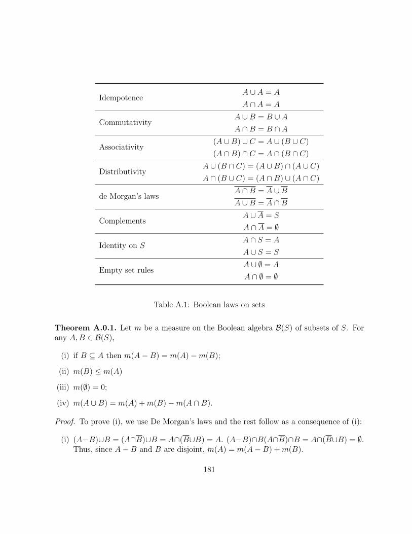
IdempotenceA ∪ A = A

A ∩ A = A

CommutativityA ∪B = B ∪ AA ∩B = B ∩ A

Associativity(A ∪B) ∪ C = A ∪ (B ∪ C)

(A ∩B) ∩ C = A ∩ (B ∩ C)

DistributivityA ∪ (B ∩ C) = (A ∪B) ∩ (A ∪ C)

A ∩ (B ∪ C) = (A ∩B) ∪ (A ∩ C)

de Morgan’s lawsA ∩B = A ∪BA ∪B = A ∩B

ComplementsA ∪ A = S

A ∩ A = ∅

Identity on SA ∩ S = A

A ∪ S = S

Empty set rulesA ∪ ∅ = A

A ∩ ∅ = ∅

Table A.1: Boolean laws on sets

Theorem A.0.1. Let m be a measure on the Boolean algebra B(S) of subsets of S. Forany A,B ∈ B(S),

(i) if B ⊆ A then m(A−B) = m(A)−m(B);

(ii) m(B) ≤ m(A)

(iii) m(∅) = 0;

(iv) m(A ∪B) = m(A) +m(B)−m(A ∩B).

Proof. To prove (i), we use De Morgan’s laws and the rest follow as a consequence of (i):

(i) (A−B)∪B = (A∩B)∪B = A∩(B∪B) = A. (A−B)∩B(A∩B)∩B = A∩(B∪B) = ∅.Thus, since A−B and B are disjoint, m(A) = m(A−B) +m(B).

181

(ii) m(A−B) ≥ 0 so it follows immediately from (i).

(iii) m(∅) = m(S − S) = m(S)−m(S) = 0, where we used (i).

(iv) A∪B = (A∪B)∪∅ = (A∪B)∪[(A∩B)−(A∩B)] = [A−(A∩B)]∪[B−(A∩B)]U(A∩B).Therefore, m(A ∪ B) = m(A) − m(A ∩ B) + m(B) − m(A ∩ B) + m(A ∩ B) =m(A) +m(B)−m(A ∩B).

The notion of probability

When a set S represents the possible outcomes of some experiment, we say that S is thesample space for the experiment. An event is a subset of outcomes in the sample space S.More specifically, it is the subset of outcomes for which a certain proposition holds true.

Kolmogorov’s axioms states that for every event E in an experiment, we can assign anumber p(E) called the probability of event E such that

(i) p(E) is non-negative,

(ii) an event corresponding to the entire sample space has p(S) = 1, and

(iii) for disjoint events A and B, that is, A ∩B = ∅, then

p(A ∪B) = p(A) + p(B). (A.2)

But these properties are nothing more than a measure p on the Boolean algebra B(S) ofsubsets of S with unit total mass. The triple {S,B(S), p} denotes the probability spacewith sample space S, space of events B(S) and probability measure p.

Let A,B ∈ B(S). The probability measure p on B(S) has the following properties:

1. p(∅) = 0, p(S) = 1.

2. 0 ≤ p(A) ≤ p(S).

3. p(A ∪B) = p(A) + p(B)− p(A ∩B).

4. p(A) = 1− p(A).

182

5. p(A) ≤ p(B) whenever A ⊆ B.

6. Let E = {E1, . . . , EN} be a partition of S into N disjoint subsets, i.e., Ei ∩ Ej = ∅for any i 6= j, then

N∑j=1

p(Ej) = 1. (A.3)

Properties (i) to (iii) are conditions on p that satisfy Kolmogorov’s axioms.

The main role of p is to assign a weight to each event in B(S) based on its plausibility,in which case probability-one means an event is certain while probability-zero means anevent is never going to occur.

When probabilities are determined with the assumption that certain events occurred,they are called conditional probabilities. The conditional probability P (A|B) is the proba-bility of event A given that event B is true. Conditional probabilities are especially impor-tant in Bayesian inference, where all probabilities are conditional on some prior knowledge,which are then updated when new information is acquired.

Intuitively, we want conditional probabilities to have the following properties:

(i) Since it is still a measure but only on a smaller sample space, we expect p(B|B = 1and p(∅|B) = 0.

(ii) For any A ∈ B(S), p(A−B|B) = p(A ∩B) = 0.

(iii) p as a measure also means

p(A|B) = p[(A ∩B) ∪ (A ∩B)|B]

= p(A ∩B|B) + p(A−B|B)

= p(A ∩B|B).

(A.4)

Thus, if we know the values for p(A|B) for all subsets A ⊆ B then we know everythingabout the probabilities conditioned on B.

(iv) If E1 and E2 represent disjoint events then

p(E1|B) + p(E2|B) = p(E1 ∪ E2|B). (A.5)

183

These properties are satisfied if we define the conditional probability of A given B to be

p(A|B) =p(A ∩B)

p(B)(A.6)

for p(B) > 0.

Conditional probabilities allow us to decompose probabilities of intersections into prod-ucts of probabilities:

p(A1∩A2∩ . . .∩AN) = p(A1)p(A2|A1)p(A3|A1∩A2) . . . p(AN |A1∩A2∩ . . .∩AN−1). (A.7)

For unions of events, the most important case is when we consider a partition of S, thatis, {Ei : i = 1, 2, . . . , N} such that Ei ∩ Ej = ∅ for i 6= j and

⋃Ni=1Ei = S. Using disjoint

additivity,

p(A) = p

[N⋃i=1

(Ei ∩ A)

]=

N∑i=1

p(Ei ∩ A), (A.8)

which leads us to the law of total probability:

Theorem A.0.2 (Law of total probability). Let {S,B(S), p} be a probability space and{Ei : i = 1, 2, . . . , N} be a partition of S into disjoint subsets. The probability of event Ais given by

p(A) =N∑i=1

p(Ei)p(A|Ei). (A.9)

In many practical situations, the probability of an event is conditioned on some hiddenstates of the experiment. If we have some beliefs about the likelihood of each hidden state,the law of total probability tells us how to compute the event’s probability.

Finally, we note that two events A and B are said to be statistically independent if

p(A ∩B) = p(A)p(B), (A.10)

which implies that p(A|B) = p(B) and p(B|A) = p(A). That is, the plausibility of A isnot affected by B, and vice-versa.

Bayesian updating

In daily life, we are interested in the values of all sorts of quantities. However, manyof them are difficult to determine directly and must be inferred from various forms of

184

evidence. With probability models, the situation is reversed: there is a model for assigningprobabilities to events provided a certain hypothesis is true. When there is available dataserving as evidence, the aim becomes assessing the probability that the initial hypothesisis correct. Unfortunately, there is no unique, objective way to accomplish this. However,if we are willing to assign prior probabilities based on any subjective judgements, thenprobability theory tells us how to revise our initial beliefs in the face of new information.

Suppose we have some initial hypothesis represented by set H and with probabilityp(H). From the inclusion-exclusion principle, p(H) = 1− p(H). Now suppose we observesome evidence which we call event E. Also, there is a known probability model whichprovides us with values for the probabilities p(E|H) and p(E|H). To update the probabilityof H from its prior value p(H) to some posterior value p(H|E), we could use

p(H|E) =p(H ∩ E)

p(E)(A.11)

but generally we do not know any of the probabilities on the right-hand side. Instead wecompute

p(H ∩ E)p(H)p(E|H) (A.12)

and use the law of total probability for the partition {H,H} to obtain

p(H|E) =p(H)p(E|H)

p(H)p(E|H) + p(H)p(E|H). (A.13)

If there is more than a single hypothesis to consider (Hj, j = 1, . . . , N), we would use

p(Hj|E) =p(Hj)p(E|Hj)∑Nk=1 p(Hk)p(E|Hk)

. (A.14)

Eq. (A.14) is called Bayes’ theorem and it describes the rational way for modifying initialprobabilities to account for new evidence.

Interpreting probabilities

What exactly do we mean when we say that the probability of event E is p(E)? Oneof the earliest known attempts to rigorously define probabilities is due to Pierre-SimonLaplace. It is called the classical theory of probability and was developed from an analysisof various games of chance. Its main idea is the principle of symmetry for all possible

185

outcome, provided those outcomes are reasonably deemed equally likely. Formally, if anexperiment can yield one of N mutually exclusive, equally possible outcomes, and NA ofthose outcomes are associated with event A then we define the probability of event A as

p(A) =NA

N. (A.15)

It is clear that the definition is faulty: first, it seems to work only in the cases with finiteoutcomes but more importantly, it is difficult to see how one avoids running into a circularargument when trying to identify outcomes that are equally likely. Nevertheless, there arecertain instances when it seems intuitively justified, like when we consider ensembles instatistical mechanics, where microstates that correspond to the same macrostate, which areindistinguishable with regard to their thermodynamic properties, are deemed equiprobable.

Arguably the most widely accepted interpretation of probabilities is in terms of relativefrequencies. The idea behind frequentism is that the probability of an event is reflected byits relative frequency over the course of many repetitions of the same experiment. If NA

denotes the number of occurrences of event A then if

limN→∞

NA

N= pA (A.16)

we say that the probability of A is pA.

The frequentist point of view has its own problems, the main one being the impossibilityof performing identical experiments infinitely many times to confirm that the relativefrequency indeed tends to the probability. It may be argued that the limit can be thoughtof as the limit for an imagined infinite ensemble of identically prepared, independentlydistributed systems in thought experiments. Still, you run into the problem of justifyingwhy a certain limit is guaranteed when there is no way to actual observe the infinite relativefrequency. For instance, say we observe that a coin flipped 20 times yields 10 heads and10 tails. We would be inclined to believe that the coin is fair, with equal probability forheads or tails. But if is not inconceivable that if you actually flip it a million times, youwould get 600,000 heads, which would hardly make the coin a fair one. Without actuallydoing the experiments, it is impossible to verify either way.

There are some attempts to think of relative frequency in terms of a finite number oftrials but the relative frequency becomes ambiguous. Even with a marginal increase inthe number of trials, relative frequencies can change significantly and thus, there is nodiscernible way to determine a unique probability.

One can choose to move away from relative frequencies to the camp of propensitytheorists, who contend that the observed relative frequencies are mere indicators of some

186

physical property of the system to generate the particular outcome associated with it. Theidea is to think of probability as an objective property akin to mass or electric charge.However, the problem with the propensity view is without expounding on the features ofthat physical property, then propensity becomes just a different name for probability.

Finally we have the camp of subjectivists, whose basic tenets is that all probabilitiesare conditional on an agent’s subjective degrees of beliefs resulting from assessing the un-certainty surrounding a particular experiment. Whereas the probability associated withpropensity would be called objective chance, subjectivists would refer to it as a credencefunction.Subjectivists are sometimes called Bayesians, since the methods for updating prob-abilities are often performed under the framework of subjective prior probabilities. Theidea behind Bayesian probabilities is to assign probabilities that may be subjective but arenonetheless consistent. One way to motivate this is through the Dutch book argument forevaluating gambling odds, which we describe in the next section.

The rational gambler

A simple way to explain subjective probabilities is to argue that probability assignmentsare correct only in so much as they are developed from rational decision making. Inthis way, probabilities are really the generalization of logical thinking in the presence ofuncertainty. Just as logic is concerned with valid reasoning about propositions but does notsay anything about the truth values of those propositions, probability theory is concernedwith proper methods for dealing with uncertainty without making a commitment to a fixedquantification of that uncertainty. For concreteness, it is conventional to use the exampleof a betting scenario.

Imagine there is a bookmaker who offers a bet for some event E to occur. A bettorwilling to accept this bet has to pay a stake of pX dollars up front. The bookmaker pays Xif E happens and nothing if it does not. In terms of gambling odds, the bettor is making abet at odds of (1−p)/p is to 1. Recall that for odds of x to y, it means the bettor is willingto bet a fraction x/(x+ y) of his money that he will win the bet. Thus, the probability ofthe bettor winning is given by

p =x

x+ y. (A.17)

Now since the bookmaker chooses the value of X, he might try to choose it so that thebettor never wins. This is called an inconsistent betting scenario, and rational gamblerwould never participate in that.

187

The important quantity to consider is the bettor’s average gain G,

G = X − pX = (1− p)X, (A.18)

which is the net amount the bettor earns if he wins.

Suppose that event E has two outcomes called ‘yes’ and ‘no’, with associated winningsof Y and N , respectively. Let p(E = yes) = q and p(E = no) = 1− q with correspondingstakes qY and (1− q)N . Normally the bookmaker doesn’t want to pay out anything if Edoes not happen so he can choose N = 0. If E = yes then Gyes = (1− q)Y ; if E = no thenGno = −qY since the bettor has to pay for the stake in any situation.

The bookmaker can make both Gyes and Gno negative except when 1 − q and q havethe same sign, which implies that

1− qq

> 0. (A.19)

If q < 0 then 1 − q < 0 or q > 1, which is false by assumption. So q > 0, from which itfollows that 1− q > 0 or q < 1, that is,

0 < q < 1. (A.20)

The argument can be extended to include both certain q = 1 and impossible q = 0 eventsif the gambler wants to avoid the situation where he believes E might occur but his bestgain is zero. The analysis can be extended to demonstrate other properties of probabilitiessuch as disjoint additivity, when one considers betting on mutually exclusive events, andBayes’ theorem, when we consider conditional bets.

We emphasize that only the gambler assigns probabilities. The only concern of thebookmaker is to persuade the gambler to place bet in situations that are not so favorableto the bettor. The Dutch book argument is not an analysis of the competition betweengambler and bookmaker; rather it is entirely about consistent betting behavior for thegambler alone. The only assumption is that a rational gambler will always avoid a scenariowhere he can never win.

188

Appendix B

Convex sets in real Euclidean spaces

The state space of a typical algebra has a natural convex structure: one can use probabilitiesµj to obtain mixtures ∑

j

µjωj (B.1)

of states ωj. If we assume finite dimensional A then the S(A) is generally a convex subsetof a finite-dimensional real space.

A subset K of RN is convex if the line segments joining points of K lie in K.

For any arbitrary subset X ∈ RN , we can form its convex hull

Conv(X) = {∑j

µjxj : xj ∈ X,µj ≥ 0,∑j

µj = 1}. (B.2)

Consider the convex boundary ∂CK of a closed, compact subset of RN , it is the set ofextreme points of K that admit only trivial decompositions in K. More explicitly, k isextreme if

k = λk1 + (1− λ)k2, 0 ≤ λ ≤ 1, k1, k2 ∈ K =⇒ k1 = k2 = k. (B.3)

Two basic results in convex theory are the Krein-Milman theorem and Caratheodory’stheorem. The Krein-Milman theorem [84] states that a compact convex set K ∈ RN is theclosed convex hull of its extreme points. Caratheodory’s theorem states that every pointin a convex subset of RN admits a mixture of at most N + 1 points.

A distinguished class of compact convex sets of RN are the simplices ∆N , which arecharacterized by the unique decomposition of any point in ∆N into a convex combinationof extreme points.

189

An important class of convex sets is the set of bistochastic matrices. These are squarematrices Bjk of dimension N such that for all j, k

Bjk ≥ 0,∑j

Bij =∑k

Bkl = 1. (B.4)

Bistochastic matrices define a class of Markov processes with transition probabilities thatleave the uniform distribution invariant. Birkhoff’s theorem says that the extreme pointsof the set of bistochastic matrices are the set of permutation matrices.

Probabilities can be stochastically ordered, that is, given probability distributions ~pand ~q, we say that p majorizes q if for all j = 1, 2, . . . , N

max{p1 + p2 + ...+ pj} ≥ max{q1 + q2 + . . .+ qj}. (B.5)

Hardy-Littlewood-Polya theorem defines this order relation as some measure of mixedness:~p � ~q if and only iff ~q is obtained from ~p by a convex combination of permutations, i.e.,

~q = B~p (B.6)

where B is some bistochastic matrix.

Majorized ordering is important in comparing certain quantities such as Shannon en-tropy H(~p)

H(~p) = −N∑j=1

pj ln pj (B.7)

which is a concave function

H(α~p+ (1− α)~q) ≥ αH(~p) + (1− α)H(~q). (B.8)

By virtue of Hardy-Littlewood-Polya theorem and since the entropy is invariant underpermutations,

H(~q) ≥ H(~p) (B.9)

whenever ~q = B~p for bistochastic B. Thus, more mixed probability distributions havehigher entropy.

190

Appendix C

Basic facts about linear operators

Here is a quick reminder of properties of linear operators that are relevant in the contextof quantum mechanics.

1. We can write linear operators on a Hilbert space in the form

A =d∑i,j

aij|ai〉〈aj| (C.1)

by including enough terms in the decomposition, which is possible since

B(H) = H⊗H∗. (C.2)

2. A linear operator A ∈ B(H) is diagonalized by some unitary matrix U ,

UU † = U †U = I, (C.3)

if and only if it is normal, that is,

[A,A†] = AA† − A†A = 0. (C.4)

3. Any normal operator can be expressed in the form

A =r∑i=1

ai|ai〉〈ai| (C.5)

where the set {|ai〉} consists of an orthogonal set of eigenvectors corresponding tothe r nonzero eigenvalues ai of A. Eq. (C.5) is known as the spectral decompositionof A.

191

4. An operator P is said to be positive semidefinite if

〈ψ|P |ψ〉 ≥ 0 (C.6)

for all |ψ〉 ∈ H. For the eigenvectors of A, this means that the eigenvalues of A areall non-negative. Alternatively, one can write P as

P = AA† (C.7)

for some matrix A ∈ B(H). If we choose A to be a lower triangular matrix withstrictly positive diagonal entries, then Eq. (C.7) is the Cholesky decomposition ofP . Any convex combination of positive operators is again a positive operator, whichimplies that the set P of all positive operators form a convex cone.

5. Any square complex matrix A can be decomposed into the form

A = UP (C.8)

where U is a unitary matrix and P is a positive operator. This is the matrix analogof polar decomposition for complex numbers,

z = reiθ (C.9)

where r ≥ 0 and 0 ≤ θ ≤ 2π for any z ∈ C.

6. One way to impose positivity conditions on a parameterized matrix is by consideringthe spectrum of an arbitrary operator A derived from its characteristic polynomial

det (aI − A) = aN − c1aN−1 + c2a

N−2 + . . .+ (−1)NcN = 0. (C.10)

Recall that the coefficients ci of this polynomial can be expressed in terms of sym-metric functions of the roots, which are actually the eigenvalues a of A in this case,through formulas called Newton-Girard identities [72]:

Tr(Ak)

+ cN−1Tr(Ak−1

)+ . . .+ cN−k+1Tr (A) = −kcN−k, (1 ≤ k ≤ N), (C.11)

Tr(Ak)

+ cN−1Tr(Ak−1

)+ . . .+ c0Tr

(Ak−N

)= 0, (k > N). (C.12)

192

Appendix D

Measuring distances betweenprobability distributions

There are two important notions of distances connected with probabilities: the more tra-ditional Euclidean distance when probability distributions are considered as vectors in areal linear space, and the perhaps lesser known notion of statistical distance, which distin-guishes probability distributions that are almost identical in light of uncertainty.

Hilbert-Schmidt distance between probability distribu-

tions

Consider an experiment with N possible outcomes or some random variable X correspond-ing to it, with range {xi : i = 1, 2, . . . , N}. Let the probability for each outcome be givenby

p(X = xi) = pi (D.1)

In many situations, the outcomes themselves are not very significant. What matters moreis the probability distribution p(X) treated as a collection of N numbers p(i) such thatp(i) ≥ 0,

∑i p(i) = 1. We consider these numbers to be the components of vector ~p that

belongs to some N -dimensional real vector space. Technically the probabilities reside in an(N − 1)-dimensional space because of the linear constraint associated with normalization.Nevertheless, we keep to the components p(i) and consider the set of all probabilities,known as the probability simplex, as embedded on RN . One reason to do this is that

193

it allows to adopt the usual geometric notions in real Euclidean spaces such as norms ordistances.

Given the Cartesian coordinates p = (p1, p2, . . . , PN) and q = (q1, q2, . . . , qN) of twoprobability distributions, the inner product is the usual dot product for a real EuclideanN -space

〈~p, ~q〉 = ~p · ~q =N∑i=1

piqi. (D.2)

This natural comes with a definition for the distance between ~p and ~q,

D(~p, ~q) = D(~q, ~p) =

√√√√ N∑i=1

(qi − pi)2. (D.3)

and the length of a probability distribution

||~p|| =

√√√√ N∑i=1

p2i . (D.4)

Mathematically, a probability distribution is simply a measure on a sample space con-strained to have unit total mass. In its vector space representation, the probability spacecorresponds to a set of points that forms a convex set. For instance, we know that theentire set of N -outcome probabilities forms an (N − 1)-dimensional simplex ∆N−1, whichwhen embedded in a Euclidean space is simply a regular hypertriangle lying on the hyper-plane given by p1 + p2 + . . . + pN = 1, where the standard basis vectors correspond to itsvertices.

Statistical geometry and the Fubini-Study metric

When we represent density operators using real vectors, it is natural to assume that thethese vectors are embedded in a d2-dimensional real Euclidean space, so that we can talkabout how two states are different from each other in terms of Euclidean or Hilbert-Schmidt distances. There is, however, an alternate way of comparing a pair of states, onethat quantifies how easy or hard they are to distinguish from each other from measurementresults. Here we review the situation discussed by Wootters in Ref. [130].

194

Consider a finite ensemble of identically prepared quantum systems analyzed by a fixedmeasuring device. The relative frequencies we obtain from measurements will typicallybe different from the actual probabilities if the preparation is fully known. Because ofthis statistical uncertainty, it is not always possible to distinguish between two marginallydifferent preparations in a limited number of trials. This leads to the notion of statisticaldistance between quantum states, which involves counting the number of distinguishablestates between any pair of states, where distinguishability is determined entirely by thesize of statistical fluctuations.

In general, for an experiment with d possible outcomes, the relative frequencies aredistributed according to a multinomial distribution, which is approximately Gaussian in thelimit of very large N . Two probability distributions ~p and ~q are said to be distinguishablein N trials, if and only if

√N

2

[d∑i=1

(∆pi)2

pi

]1/2

> 1 (D.5)

where ∆pi = pi − qi. This condition guarantees that ~p and ~q will not have overlappingregions of uncertainty.

Geometrically, the statistical distance between ~p and ~q can be computed as the lengthof a smooth curve connected ~p and ~q; in fact, it is the one with minimum length

L = min~p(t)

1

2

∫ 1

0

dt

√√√√ d∑i=1

1

pi(t)

[dpi(t)

dt

]2

(D.6)

where ~p(t) is a parameterized curve such that ~p(0) = ~p and ~p(1) = ~q.

Let xi =√pi and yi =

√qi. Then L becomes

L =

∫ 1

0

dt

√√√√ d∑i=1

(dxidt

)2

, (D.7)

which we recognize as the Euclidean length in the space of ~x and ~y. The requirement thatthe curve ~p(t) must lie within the space of probabilities is imposed by the constraint

d∑i=1

pi(t) =d∑i=1

x2i (t) = 1, (D.8)

which means that the curve ~x(t) must lie on the unit hypersphere in the Euclidean spaceof ~x-type vectors.

195

The statistical distance, also called the Bhattacharya distance, between probabilitydistributions ~p and ~q is therefore the shortest distance between two points ~x and ~y alonga unit sphere provided that xi =

√pi and yi =

√qi. Formally, we would write

Dst(~p, ~q) = arccos

(d∑i=1

√pi√qi

). (D.9)

Now consider two quantum states |ψ〉 and |φ〉 in a d-dimensional Hilbert space. Forsome orthonormal basis {|1〉 , . . . , |d〉}, we can write

|ψ〉 =d∑i=1

αi |i〉 , |φ〉 =d∑j=1

βj |j〉 . (D.10)

The statistical distance between |ψ〉 and |φ〉 can then be computed from the probabilities|αi|2 and |βi|2,

Dst (|ψ〉 , |φ〉) = arccosd∑i=1

|αi||βi| = arccos2∑i=1

|〈i|ψ〉||〈φ|i〉|. (D.11)

The distance Dst (|ψ〉 , |φ〉) reaches its maximum value when the measurement projects ontoone of the basis vectors |i〉 that is also an eigenstate of the observable being measured, e.g.if we were trying to measure observable A, which has spectral decomposition

A =d∑i=1

ai|i〉〈i|, (D.12)

then the absolute statistical distance D∗st is

D∗st (|ψ〉 , |φ〉) = arccos |〈φ|ψ〉|. (D.13)

This is actually the exact same expression for the angle between two rays |ψ〉 and |φ〉in Hilbert space. More specifically, the angle represents the geodesic length of a line inthe projective Hilbert space CPd−1, more commonly known as the Fubini-Study metric.Thus, we have just established that the Fubini-Study metric measures the experimentaldistinguishability of pure quantum states in terms of the statistical distance between theprobability distributions they generate from a measurement with a finite number of trials.

196

Appendix E

Theory of filters and transitionprobabilities

John von Neumann’s treatise on quantum mechanics established the most widely acceptedframework for the theory, where each quantum system is associated with a Hilbert spaceH, unit vectors |ψ〉 ∈ H specifies a possible state, and self-adjoint operators A ∈ B(H)represent observables. Does this particular representation impose limits on the allowedstructure for quantum state space?

Birkhoff and von Neumann attempted to answer this question by examining the struc-ture of pure states in terms of the set of yes-no measurements, obtaining a lattice ofHilbert space projection operators with features akin to a logical system. To understandthe projection lattice operationally, we model the yes-no measurements as filters that selectcertain beams of particles, with ‘yes’ for particles that pass through a filter and ‘no’ forthose absorbed, as shown in Fig. E.1a.

Consider 2 filters a, b ∈ Q placed in sequence like in Fig. E.1b. In general, the intensityof the beam that passes through a will be diminished further by filter b and the relativedecrease is constant in certain cases. For instance, the intensity of light is reduced bycos2 θ as it pass through to linear polarizers oriented at an angle θ relative to each other.In analogy with light, we can introduce an absorption coefficient for every pair of filterscorresponding to the transition probability of going from state a to b, and vice-versa. Wesay that an absorption coefficient p(a, b) exists between filters a, b ∈ Q if the relativedecrease in intensity for a beam exiting a and passing into b is p(a, b) and is the same whenthe a and bs are interchanged. Having a definite absorption coefficient for every pair offilters characterizes a geometric property for filters. For example, orthogonal filters have

197

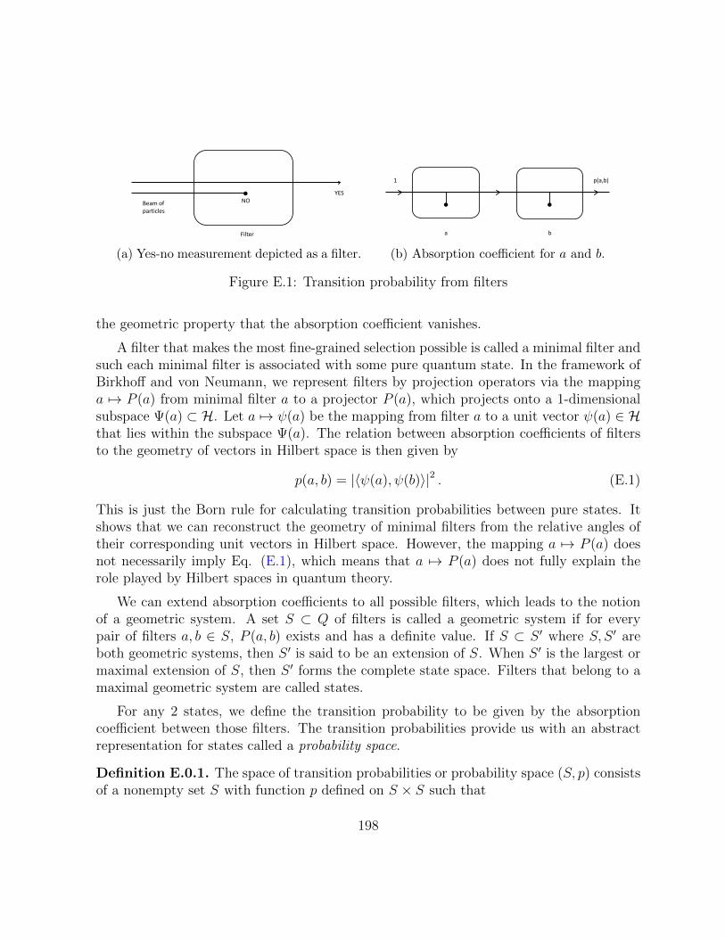
Filter

Beam of particles

NO YES

(a) Yes-no measurement depicted as a filter.

a b

1 p(a,b)

(b) Absorption coefficient for a and b.

Figure E.1: Transition probability from filters

the geometric property that the absorption coefficient vanishes.

A filter that makes the most fine-grained selection possible is called a minimal filter andsuch each minimal filter is associated with some pure quantum state. In the framework ofBirkhoff and von Neumann, we represent filters by projection operators via the mappinga 7→ P (a) from minimal filter a to a projector P (a), which projects onto a 1-dimensionalsubspace Ψ(a) ⊂ H. Let a 7→ ψ(a) be the mapping from filter a to a unit vector ψ(a) ∈ Hthat lies within the subspace Ψ(a). The relation between absorption coefficients of filtersto the geometry of vectors in Hilbert space is then given by

p(a, b) = |〈ψ(a), ψ(b)〉|2 . (E.1)

This is just the Born rule for calculating transition probabilities between pure states. Itshows that we can reconstruct the geometry of minimal filters from the relative angles oftheir corresponding unit vectors in Hilbert space. However, the mapping a 7→ P (a) doesnot necessarily imply Eq. (E.1), which means that a 7→ P (a) does not fully explain therole played by Hilbert spaces in quantum theory.

We can extend absorption coefficients to all possible filters, which leads to the notionof a geometric system. A set S ⊂ Q of filters is called a geometric system if for everypair of filters a, b ∈ S, P (a, b) exists and has a definite value. If S ⊂ S ′ where S, S ′ areboth geometric systems, then S ′ is said to be an extension of S. When S ′ is the largest ormaximal extension of S, then S ′ forms the complete state space. Filters that belong to amaximal geometric system are called states.

For any 2 states, we define the transition probability to be given by the absorptioncoefficient between those filters. The transition probabilities provide us with an abstractrepresentation for states called a probability space.

Definition E.0.1. The space of transition probabilities or probability space (S, p) consistsof a nonempty set S with function p defined on S × S such that

198

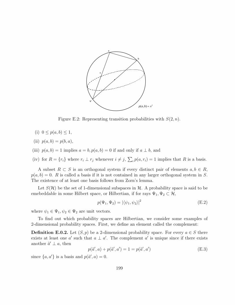
a

b

b’

x

2),( xbap =

Figure E.2: Representing transition probabilities with S(2, n).

(i) 0 ≤ p(a, b) ≤ 1,

(ii) p(a, b) = p(b, a),

(iii) p(a, b) = 1 implies a = b, p(a, b) = 0 if and only if a ⊥ b, and

(iv) for R = {ri} where ri ⊥ rj whenever i 6= j,∑

i p(a, ri) = 1 implies that R is a basis.

A subset R ⊂ S is an orthogonal system if every distinct pair of elements a, b ∈ R,p(a, b) = 0. R is called a basis if it is not contained in any larger orthogonal system in S.The existence of at least one basis follows from Zorn’s lemma.

Let S(H) be the set of 1-dimensional subspaces in H. A probability space is said to beemebeddable in some Hilbert space, or Hilbertian, if for rays Ψ1,Ψ2 ⊂ H,

p(Ψ1,Ψ2) = |〈ψ1, ψ2〉|2 (E.2)

where ψ1 ∈ Ψ1, ψ2 ∈ Ψ2 are unit vectors.

To find out which probability spaces are Hilbertian, we consider some examples of2-dimensional probability spaces. First, we define an element called the complement:

Definition E.0.2. Let (S, p) be a 2-dimensional probability space. For every a ∈ S thereexists at least one a′ such that a ⊥ a′. The complement a′ is unique since if there existsanother a′ ⊥ a, then

p(a′, a) + p(a′, a′) = 1 = p(a′, a′) (E.3)

since {a, a′} is a basis and p(a′, a) = 0.

199

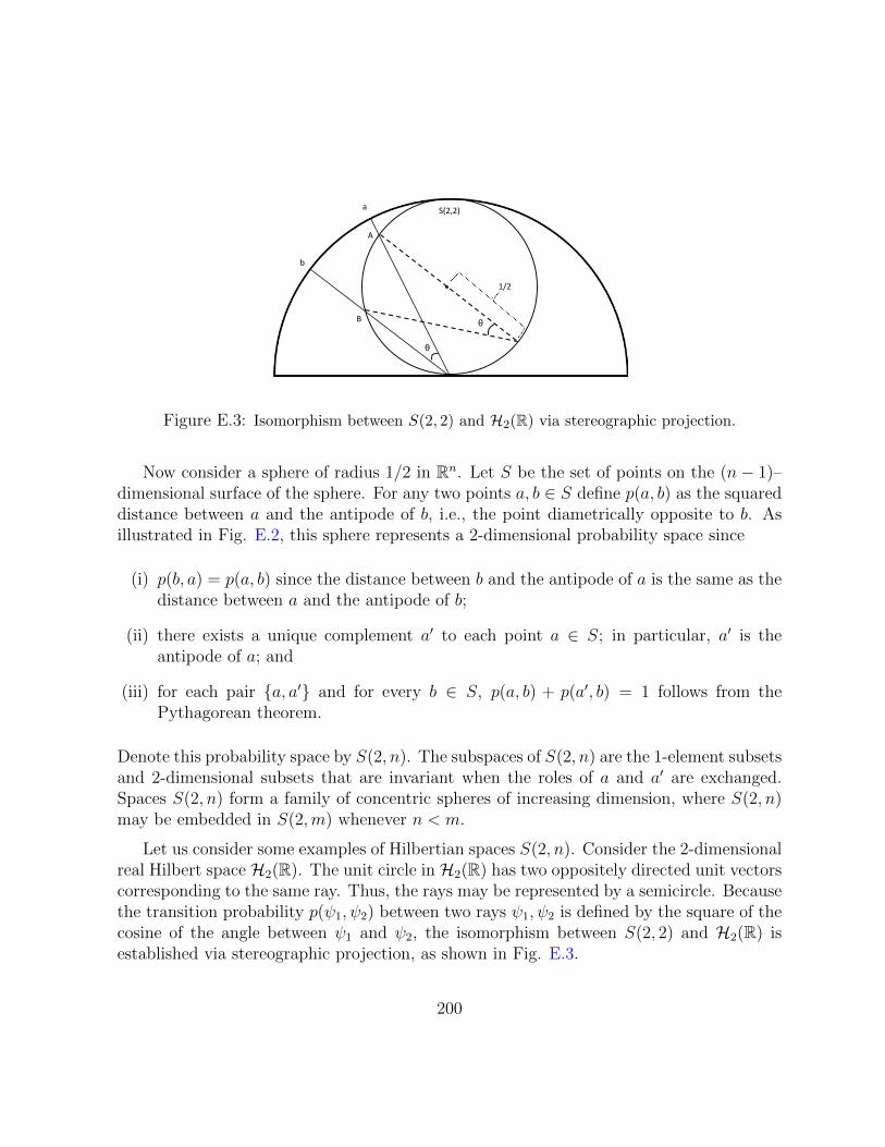
a

b

A

B

θ

θ

1/2

S(2,2)

Figure E.3: Isomorphism between S(2, 2) and H2(R) via stereographic projection.

Now consider a sphere of radius 1/2 in Rn. Let S be the set of points on the (n− 1)–dimensional surface of the sphere. For any two points a, b ∈ S define p(a, b) as the squareddistance between a and the antipode of b, i.e., the point diametrically opposite to b. Asillustrated in Fig. E.2, this sphere represents a 2-dimensional probability space since

(i) p(b, a) = p(a, b) since the distance between b and the antipode of a is the same as thedistance between a and the antipode of b;

(ii) there exists a unique complement a′ to each point a ∈ S; in particular, a′ is theantipode of a; and

(iii) for each pair {a, a′} and for every b ∈ S, p(a, b) + p(a′, b) = 1 follows from thePythagorean theorem.

Denote this probability space by S(2, n). The subspaces of S(2, n) are the 1-element subsetsand 2-dimensional subsets that are invariant when the roles of a and a′ are exchanged.Spaces S(2, n) form a family of concentric spheres of increasing dimension, where S(2, n)may be embedded in S(2,m) whenever n < m.

Let us consider some examples of Hilbertian spaces S(2, n). Consider the 2-dimensionalreal Hilbert space H2(R). The unit circle in H2(R) has two oppositely directed unit vectorscorresponding to the same ray. Thus, the rays may be represented by a semicircle. Becausethe transition probability p(ψ1, ψ2) between two rays ψ1, ψ2 is defined by the square of thecosine of the angle between ψ1 and ψ2, the isomorphism between S(2, 2) and H2(R) isestablished via stereographic projection, as shown in Fig. E.3.

200

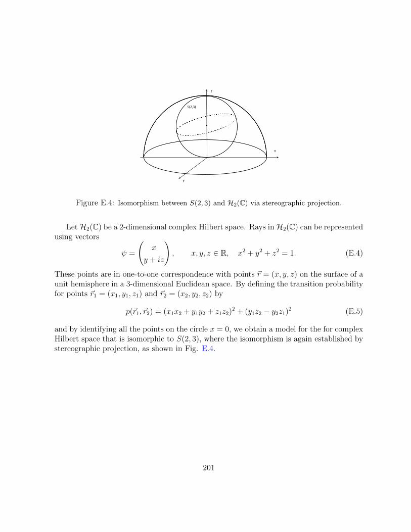
S(2,3)

z

y

x

Figure E.4: Isomorphism between S(2, 3) and H2(C) via stereographic projection.

LetH2(C) be a 2-dimensional complex Hilbert space. Rays inH2(C) can be representedusing vectors

ψ =

(x

y + iz

), x, y, z ∈ R, x2 + y2 + z2 = 1. (E.4)

These points are in one-to-one correspondence with points ~r = (x, y, z) on the surface of aunit hemisphere in a 3-dimensional Euclidean space. By defining the transition probabilityfor points ~r1 = (x1, y1, z1) and ~r2 = (x2, y2, z2) by

p(~r1, ~r2) = (x1x2 + y1y2 + z1z2)2 + (y1z2 − y2z1)2 (E.5)

and by identifying all the points on the circle x = 0, we obtain a model for the for complexHilbert space that is isomorphic to S(2, 3), where the isomorphism is again established bystereographic projection, as shown in Fig. E.4.

201

Appendix F

Projective geometry of quantumphase space

Most theories in physics are explicitly formulated in geometric terms. Examples includeclassical mechanics based on symplectic geometry, general relativity based on Riemannianmanifolds, and Yang-Mills theory based on fiber bundles. On the other hand, the tradi-tional language of quantum mechanics is linear algebra and functional analysis. In 1979,Tom Kibble showed that quantum mechanics can be cast in Hamiltonian form, similar toclassical mechanics, but different in that the underlying phase space is complex projectiveHilbert space. This phase space geometry offers new insights into various aspects of quan-tum mechanics such as linear superposition, uncertainty relations, geometric phases, andentanglement.

The space of pure quantum states is complex projective Hilbert space CPd−1, wherepoints correspond to rays in the Hilbert space Hd. In finite dimensions, Hd

∼= Cd, wherenormalized vectors define a sphere

S2d−1 = {|ψ〉 ∈ Cd : 〈ψ|ψ〉 = 1}. (F.1)

Two points |ψ〉 and |φ〉 represent the same state if

|φ〉 = eiα |ψ〉 , α ∈ R (F.2)

so CPd−1 = S2d−1/U(1). For example, CP1 = S3/U(1) ∼= S2, which is the Bloch ball.

In general, CPd−1 is a complex space equipped with a symplectic form and a Fubini-Study metric inherited from Hilbert space. If we decompose the Hilbert space scalar

202

product into its real and imaginary parts, 〈ψ|φ〉 = R(ψ, φ) + iJ(ψ, φ) where R(ψ, φ) =Re [〈ψ|φ〉] and J(ψ, φ) = Im [〈ψ|φ〉], then

R(ψ, φ) = R(φ, ψ), J(ψ, φ) = −J(φ, ψ), J(ψ, φ) = R(ψ, iφ). (F.3)

This means that both Hilbert space and its projective counterpart are Kahler spaces.

Expressing |ψ〉 =∑

α ψα |eα〉 for some orthonormal basis {|eα〉}di=1 ⊂ Cd, the Fubini-Study metric is given by

gαβ =〈ψ|ψ〉δαβ − ψαψβ − ψβψα

〈ψ|ψ〉2, (F.4)

that is, infinitesimal distances ds are defined by

ds2 =∑α,β

gαβdψαdψβ. (F.5)

For d = 2 this is just the standard round metric on the surface of the sphere S2.

The map from S2d−1 to CPd−1 defines the so-called Hopf fibration or Hopf bundle. Thesimplest Hopf fibration is for CP1 ∼= S2, which gives rise to the projection S3 → S2. Forexample, consider a unit vector |ψ〉 for a qubit,

|ψ〉 = α |0〉+ β |1〉 . (F.6)

Define the quantitynj = 〈ψ|σj |ψ〉 (F.7)

where σj, j = 1, 2, 3 are the Pauli matrices. Then, it follows that n21 + n2

2 + n23 = 1

so |ψ〉 7→ ~n establishes a mapping from S3 to S2. For qubit Hilbert space, the Hopffibration of S3 consists of the fiber S1, which represents global phases for |ψ〉 and the basespace S2, which is the Bloch ball. To visualize the Hopf fibration, one usually performs astereographic projection from S3 to R3.

Heinz Hopf found that the maps f : S3 → S2 are characterized by a number calledHopf invariant, Hopf(f) ∈ Z. For example, the map |ψ〉 → 〈ψ|~σ |ψ〉 has Hopf invariant of1. Any two maps f and g such that Hopf(f) = Hopf(g) can be continuously deformed intoone another. In this case, f and g are said to be homotopically equivalent.

Another way to think about Hopf fibrations is to consider rotations of a 2-sphere em-bedded in a 3-dimensional space. Its rotation group SO(3) has a double cover that is dif-feomorphic to the 3-sphere, which can be identified with the special unitary group SU(2).

203

Any point on the 3-sphere is equivalent to a quaternion q = q0 + q1i+ q2j + q3k, which inturn is equivalent to a particular rotation Rq in three dimensions,

Rq =

1− 2(q22 + q2

3) 2(q1q2 − q0q3) 2(q1q3 + q0q2)

2(q1q2 + q0q3) 1− 2(q21 + q2

3) 2(q2q3 − q0q1)

2(q1q3 + q0q2) 2(q2q3 + q0q1) 1− 2(q22 + q2

1)

. (F.8)

The set of all possible quaternions produces the set of all possible rotations, which movesthe tip of one unit vector of such a coordinate frame (say, the z-axis vector) to all pointson a unit 2-sphere. However, fixing the z-axis vector does not specify the rotation fully:a further rotation is possible about the z-axis. Thus, the 3-sphere is mapped onto the 2-sphere, plus a single rotation. We say that the 3-sphere is the principle circle bundle overthe 2-sphere, which is a Hopf fibration. (Circle bundles are actually the natural settingfor Maxwell’s theory of electromagnetism, in which the quantization of electric charge isexhibited by cohomology groups that correspond to gauge transformations.)

Only 3 spheres can be equipped with group structures:

(i) S1 → complex numbers, C,

(ii) S3 → quaternions, ∼= SU(2),

(iii) S7 → octonions.

The Hopf fibration f : S7 → S4 gives rise to coset spaces S7/S3 which are important inquantum entanglement.

Suppose we have 2 quantum systems A and B with Hilbert spaces HA and HB. Thecomposite system AB has Hilbert space HA ⊗ HB, where ⊗ denotes the tensor product,meaning that if {|ai〉} is an orthonormal basis for HA and {|bj〉} is an orthonormal basisfor HB, then {|ai, bj〉 ≡ |ai〉 ⊗ |bj〉} forms an orthonormal basis for HAB.

We say that |ψ〉 is a separable state of HAB if there exists∣∣ψA⟩ ∈ HA and

∣∣ψB⟩ ∈ HB

such that|ψ〉 =

∣∣ψA⟩⊗ ∣∣ψB⟩ . (F.9)

Otherwise, the state is entangled.

For any |ψ〉 ∈ HAB, there exists an orthonormal basis {|ei〉} ⊂ HA and {|fj〉} ⊂ HB

such that

|ψ〉 =r∑

k=1

αk |ek〉 ⊗ |fk〉 (F.10)

204

where αk > 0,∑r

k α2k = 1 and r ≤ min{n,m}. Eq. (F.10) is called the Schmidt decompo-

sition of |ψ〉. A state |ψ〉 is said to be separable if and only if there is just one term in itsSchmidt decomposition.

The most important example of entangled states are the 2-qubit Bell states∣∣Ψ±⟩ =1√2

(|01〉 ± |10〉) ,∣∣Φ±⟩ =

1√2

(|00〉 ± |11〉) , (F.11)

where {|0〉 , |1〉} is the standard basis for a qubit. The four Bell states form an orthonormalbasis in C4.

Any normalized 2-qubit state can be expressed as

|ψ〉 = α |00〉+ β |01〉+ γ |10〉+ δ |11〉 , |α|2 + |β|2 + |γ|2 + |δ2| = 1. (F.12)

This represents a unit sphere S7 since α, β, δ, γ ∈ C. A 2-qubit state |φ〉 is separable if itis a tensor product, i.e., if

∣∣φA⟩ = a |0〉+ b |1〉 and∣∣φB⟩ = c |0〉+ d |1〉 then

|φ〉 =∣∣φA⟩⊗ ∣∣φB⟩ = ac |00〉+ ad |01〉+ bc |10〉+ bd |11〉 . (F.13)

Thus, Eq. (F.12) is separable if and only if αδ = βγ.

If we introduce the anti-linear map E : C2 ⊗ C2 → C2 ⊗ C2,

E |ψ〉 = (σ2 ⊗ σ2) |ψ∗〉 (F.14)

where |ψ∗〉 is the complex conjugate of |ψ〉 and if we define

X0 = 〈σ3 ⊗ I〉, X3 = Re [〈E〉] (F.15)

X1 = 〈σ1 ⊗ I〉, X4 = Im [〈E〉] (F.16)

X2 = 〈σ2 ⊗ I〉, (F.17)

then∑

iX2i = 1 and so the mapping |ψ〉 → (X0, X1, X2, X3) corresponds to the Hopf

fibration S7 → S4. We note that

C(ψ) = |〈ψ|E |ψ〉 | (F.18)

is, in fact, just Wootters’ concurrence function, a widely known entanglement measure for2-qubit systems.

Note that X3 + iX4 = 2 (αδ − βγ) and X3 = X4 = 0 yield a separable state. Thereforethe Hopf map S7 → S4 is sensitive to entanglement and can be used to detect it. In partic-ular, a 2-qubit state is separable if and only if its image under the Hopf map belongs to the2-dimensional sphere defined by the intersection of S4 with the 3-dimensional hyperplanedefined by X3 = 0 = X4.

205

References

[1] J. Anandan. A geometric approach to quantum mechanics. Found. Phys., 21:1265–1284, 1991.

[2] D. Applebaum. Probability and information. Cambridge University Press, Cam-bridge, 2nd edition, 2008.

[3] D. M. Appleby. SIC-POVMs and the Extended Clifford Group. J. Math. Phys.,46:052107, 2005.

[4] D. M. Appleby. Symmetric Informationally Complete Measurements of ArbitraryRank. Opt. Spectr., 103:416, 2007.

[5] D. M. Appleby. Properties of the extended Clifford group with applications to SIC-POVMs and MUBs. arXiv:0909.5233, 2009.

[6] D. M. Appleby, H. Dang, and C. A. Fuchs. Symmetric Informationally-CompleteQuantum States as Analogues to Orthonormal Bases and Minimum-UncertaintyStates. arXiv:0707.2071, 2007.

[7] D. M. Appleby, Steven T. Flammia, and Christopher A. Fuchs. The Lie AlgebraicSignificance of Symmetric Informationally Complete Measurements. J. Math. Phys.,52:022202, 2011.

[8] D. M. Appleby, A. Ericsson, and C. A. Fuchs. Properties of QBist State Spaces.Found. Phys., 41:564–579, 2011.

[9] J. S. Bell. On the problem of hidden variables in quantum mechanics. Rev. Mod.Phys., 38:447–452, 1966.

[10] J.S. Bell. Speakable and Unspeakable in Quantum Mechanics: Collected Papers onQuantum Philosophy. Cambridge University Press, Cambridge, 2004.

206

[11] E. G. Beltrametti and S. Bugajski. Effect algebras and statistical physical theories.J. Math. Phys., 38:3020–31, 1997.

[12] I. Bengtsson and H. Granstrom. The Frame Potential, on Average. Open Sys. &Information Dyn., 16:145, 2009.

[13] I. Bengtsson, S. Weis, and K. Zyczkowski. Geometry of the set of mixed states: anapophatic approach. In P. Kielanowski, S. T. Ali, A. Odzijewicz, M. Schlichenmaier,and T. Voronov, editors, Geometric Methods in Physics XXX Workshop 2011, Trendsin Mathematics, pages 175–197, Basel, 2013. Springer.

[14] I. Bengtsson and K. Zyczkowski. Geometry of Quantum States. Cambridge UniversityPress, Cambridge, 2006.

[15] Ingemar Bengtsson. From SICs and MUBs to Eddington. J. Phys. Conf. Ser.,254:012007, 2010.

[16] Ingemar Bengtsson, Stephan Weis, and Karol Zyczkowski. Geometry of the set ofmixed quantum states: An apophatic approach. arXiv:1112.2347, 2011.

[17] G. Birkhoff and J. von Neumann. The logic of quantum mechanics. Ann. of Math.,37:823–843, 1936.

[18] Niels Bohr. The Quantum Postulate and the Recent Developments of Atomic Theory.Nature, 121:580–590, 1928.

[19] D. Bonneau, M. Lobino, P. Jiang, C. M. Natarajan, Michael G. Tanner, R. H. Had-field, S. N. Dorenbos, V. Zwiller, M. G. Thompson, and J. L. O’Brien. Fast path andpolarisation manipulation of telecom wavelength single photons in lithium niobatewaveguide devices. Phys. Rev. Lett., 108:053601, 2012.

[20] Max Born. Zur Quantenmechanik der Stossvorgange. Zeitschrift fur Physik, 37:863–867, 1926.

[21] D. C. Brody and L. P. Hughston. Geometric quantum mechanics. J. Geom. Phys.,38:19–53, 2001.

[22] Jeffrey Bub. Interpreting the Quantum World. Cambridge University PRess, Cam-bridge, 1999.

[23] P. Busch. Informationally complete sets of physical quantities. Int. J. Theor. Phys.,30:1217, 1991.

207

[24] C. M. Caves. Symmetric Informationally Complete POVMs. internal report, 1999.

[25] C. M. Caves, C. A. Fuchs, and R. Schack. Conditions for compatibility of quantum-state assignments. Phys. Rev. A, 65:022305, 2002.

[26] C. M. Caves, C. A. Fuchs, and R. Schack. Unknown quantum states: the quantumde Finetti representation. J. Math. Phys., 43:4537, 2002.

[27] D. Chruscinski. Geometric Aspects of Quantum Mechanics and Quantum Entangle-ment. J. Phys. Conf. Ser., 30:9–16, 2006.

[28] R. Cleve, D. Gottesman, and H.-K. Lo. How to share a quantum secret. Phys. Rev.Lett., 83:648–651, 1999.

[29] S. Colin, J. Corbett, T. Durt, and D. Gross. About SIC-POVMs and Discrete WignerDistributions. J. Opt. B, 7:S778, 2005.

[30] Hoan Bui Dang, Kate Blanchfield, Ingemar Bengtsson, and D. M. Appleby. LinearDependencies in Weyl-Heisenberg Orbits. arXiv:1211.0215, 2012.

[31] E. B. Davies and J. T. Lewis. An Operational Approach to Quantum Probability.Commun. math. Phys., 7:239–260, 1970.

[32] K. M. Davis, K. Miura, N. Sugimoto, and K. Hirao. Writing waveguides in glass witha femtosecond laser. Opt. Lett., 21(21):1729–1731, 1996.

[33] J. Du, M. Sun, X. Peng, and T. Durt. Realization of entanglement-assisted qubit-covariant symmetric-informationally-comple positive-operator-valued measurements.Phys. Rev. A, 74:042341, 2006.

[34] T. Durt, C. Kurtsiefer, A. Lamas-Linares, and A. Ling. Wigner tomography of twoqubit states and quantum cryptography. Phys. Rev. A, 78:042338, 2008.

[35] Berthold-Georg Englert. Fringe Visibility and Which-Way Information: An Inequal-ity. Phys. Rev. Lett., 77:2152–2157, 1996.

[36] Aaron Fenyes. Non-commutative probability and maximal consistent sets. Master’sthesis, University of Waterloo, Waterloo, ON, Canada, 2010.

[37] Christopher Ferrie and Joseph Emerson. Framed Hilbert space: Hanging the quasi-probability pictures of quantum theory. New J. Phys., 11:063040, 2009.

208

[38] Ronald A. Fisher. On the dominance ratio. Proc. Roy. Soc. Edinb., 42:321–341,1922.

[39] M. Fitzi, N. Gisin, and U. Maurer. A quantum solution to the byzantine agreementproblem. Phys. Rev. Lett., 87:217901, 2001.

[40] S. Flammia. On SIC-POVMs in Prime Dimensions. J. Phys. A, 39:13483, 2006.

[41] S. T. Flammia. unpublished, 2004.

[42] C. A. Fuchs. On the Quantumness of a Hilbert Space. Quant. Inf. Comput., 4:467,2004.

[43] C. A. Fuchs. QBism, the Perimeter of Quantum Bayesianism. arXiv:1003.5209, 2010.

[44] C. A. Fuchs and Asher Peres. Quantum theory needs no interpretation. PhysicsToday, 53:70, 2000.

[45] C. A. Fuchs and R. Schack. A quantum-bayesian route to quantum-state space.Found. Phys., 41:34556, 2011.

[46] Christopher A. Fuchs. Distinguishability and Accessible Information in QuantumTheory. PhD thesis, University of New Mexico, Albuquerque, 1996.

[47] Christopher A. Fuchs and Ruediger Schack. Quantum-Bayesian Coherence: TheNo-Nonsense Version. arXiv:1301.3274, 2013.

[48] Sascha Gaertner, Mohamed Bourennane, Christian Kurtsiefer, Adan Cabello, andHarald Weinfurter. Experimental demonstration of a quantum protocol for Byzantineagreement and liar detection. Phys. Rev. Lett., 100:070504, 2008.

[49] E. F. Galvao, M. B. Plenio, and S. Virmani. Tripartite entanglement and quantumrelative entropy. J. Phys. A, 33:8809, 2000.

[50] I. M. Gelfand and M. A. Naimark. On the imbedding of normed rings into the ringof operators on a hilbert space. Math. Sbornik, 12(2):197–217, 1943.

[51] A. Gleason. Measures on the Closed Subspaces of a Hilbert Space. Indiana Univ.Math. J., 6(4):885–893, 1957.

[52] C. Godsil and A. Roy. Equiangular Lines, Mutually Unbiased Bases, and Spin Mod-els. Euro. J. Combin., 30:246–62, 2009.

209

[53] D. Gottesman. Stabilizer Codes and Quantum Error Correction. PhD thesis, Cal-ifornia Institute of Technology, 1997. Available online as arXiv:quant-ph/9705052(1997).

[54] D. Gottesman. A Theory of Fault-Tolerant Quantum Computation. Phys. Rev. A,57:127, 1998.

[55] D. Gottesman. The Heisenberg Representation of Quantum Computers, pages 32–43.Proceedings of the XXII International Colloquium on Group Theoretical Methods inPhysics. International Press, Cambridge, MA, 1999.

[56] Sandeep K. Goyal, B. Neethi Simon, Rajeev Singh, and Sudhavathani Simon. Ge-ometry of the generalized Bloch sphere for qutrit. arXiv:1111.4427, 2012.

[57] M. Grassl. Computing Equiangular Lines in Complex Space. Lecture Notes in Com-puter Science, 5393:89–104, 2008.

[58] A. D. Greentree, S. G. Schirmer, F. Green, L. Hollenberg, A. R. Hamilton, and R. G.Clark. Maximizing the Hilbert space for a finite number of distinguishable quantumstates. Phys. Rev. Lett., 92:097901, 2004.

[59] S. Groeblacher, T. Jennewein, A. Vaziri, G. Weihs, and A. Zeilinger. Experimentalquantum cryptography with qutrits. New J. Phys., 8:75, 2006.

[60] S. Gudder, S. Pulmannova, S. Bugajski, and E. Beltrametti. Convex and LinearEffect Algebras. Rep. Math. Phys., 44:359–379, 1999.

[61] N. Harrigan and R.W. Spekkens. Einstein, incompleteness, and the epistemic viewof quantum states. Found. Phys., 40(2):125–157, 2010.

[62] Werner Heisenberg. Uber den anschaulichen Inhalt der quantentheoretischen Kine-matik und Mechanik. Zeitschrift fur Physik, 43:172–198, 1927.

[63] D. Hilbert, J. von Neumann, and L. Nordheim. Uber die Grundlangen der Quanten-mechanik. Mathematische Annalen, 98:1–30, 1927.

[64] J. W. P. Hirschfeld. Projective Geometries over Finite Fields. Oxford UniversityPress, Oxford, 1998.

[65] Lane P. Hughston. d=3 SIC-POVMs and Elliptic Curves. Seminar at the PerimeterInstitute. Available at http://pirsa.org/07100040/, 2007.

210

[66] W. Hunziker. A note on symmetry operations in quantum mechanics. Helve. Phys.Acta, 45:233, 1972.

[67] I. D. Ivanovic. Geometrical description of quantal state determination. J. Phys. A,14:3241, 1981.

[68] L. Jakobczyk and M. Siennicki. Geometry of Bloch vectors in two-qubit system.Phys. Lett. A, 286:383, 2001.

[69] J. M. Jauch. Foundations of Quantum Mechanics. Addison-Wesley, Reading, 1968.

[70] N. S. Jones and N. Linden. Parts of quantum states. Phys. Rev. A, 71:012324, 2005.

[71] Amir Kalev, Jiangwei Shang, and Berthold-Georg Englert. Symmetric minimal quan-tum tomography by successive measurements. Phys. Rev. A, 2012.

[72] Dan Kalman. A Matrix Proof of Newton’s Identities. Math. Mag., 73(3):313–314,October 2000.

[73] K. Kato, M. Ishii, , and Y. Inoue. Packaging of large-scale planar lightwave circuits.IEEE Trans. Compon. Packag. Manuf. Technol. B: Adv. Packag., 21(2):121–129,1998.

[74] M. Kawachi. Silica waveguides on silicon and their application to integrated-opticcomponents. Opt. Quantum Electron., 22(5):391416, 1990.

[75] M. Khatirinejad. On Weyl-Heisenberg Orbits of Equiangular Lines. J. Russ. Laser.Res., 28:333, 2008.

[76] T. W. B. Kibble. Geometrization of Quantum Mechanics. Commun. Math. Phys.,65:189–201, 1979.

[77] I. H. Kim. Quantumness, Generalized Spherical 2-Design and Symmetric Informa-tionally Complete POVM. Quant. Inf. Comp, 7:730–737, 2007.

[78] Gen Kimura. The Bloch Vector for N-Level Systems. Phys. Lett. A, 314:339, 2003.

[79] Gen Kimura and A. Kossakowski. The Bloch Vector for N-Level Systems: theSpherical-Coordinate Point of View. Open Sys. & Info. Dyn., 12:207–229, 2005.

[80] A. Klappenecker, M. Rotteler, I. Shparlinski, and A. Winterhof. On approximatelysymmetric informationally complete positive operator-valued measures and relatedsystems of quantum states. J. Math. Phys., 46:082104, 2005.

211

[81] E. Knill, R. Laflamme, and G. J. Milburn. A scheme for efficient quantum compu-tation with linear optics. Nature, 409:46 – 52, 2001.

[82] S. Kochen and E. Specker. The problem of hidden variables in quantum mechanics.J. Math. Mech., 17:59–87, 1967.

[83] Karl Kraus. States, Effects, and Operations, volume 190 of Lecture Notes in Physics.Springer-Verlag, Berlin, 1983.

[84] M. Krein and D. Milman. On extreme points of regular convex sets. Studia Mathe-matica, 9:133–138, 1940.

[85] Y. L. Lim and A. Beige. Multiphoton entanglement through a bell multiport beamsplitter. Phys. Rev. A, 71:062311, 2005.

[86] N. Linden, S. Pospecu, and P. Skrzypczyk. How small can thermal machines be?The smallest possible refrigerator. Phys. Rev. Lett., 105:130401, 2010.

[87] A. Ling, K. P. Soh, A. Lamas-Linares, and C. Kurtsiefer. Experimental polarizationstate tomography using optimal polarimeters. Phys. Rev. A, 74:022309, 2006.

[88] R. Horodecki M. Horodecki, P. Horodecki. Separability of Mixed States: Necessaryand Sufficient Conditions. Phys. Lett. A, 223:1–8, 1996.

[89] G. Mackey. Mathematical Foundations of Quantum Mechanics. W. A. Benjamin,New York, 1963.

[90] G. Mackey. Quantum Mechanics and Hilbert Space. American Math. Monthly,64:45–57, 1967.

[91] Yong-Cheng Ou Mark S. Byrd, C. Allen Bishop. General open-system quantumevolution in terms of affine maps of the polarization vector. Phys. Rev. A, 83:012301,2011.

[92] Graham D. Marshall, Alberto Politi, Jonathan C. F. Matthews, Peter Dekker, MartinAms, Michael J. Withford, and Jeremy L. OBrien. Laser written waveguide photonicquantum circuits. Opt. Exp., 17(15):12546–12554, 2009.

[93] A. Martin, A. Issautier, H. Herrmann, W. Sohler, D. B. Ostrowsky, O. Alibart, andS. Tanzilli. A quantum relay chip based on telecommunication integrated opticstechnology. New J. Phys., 12:103005, 2010.

212

[94] J. C. F. Matthews, A. Politi, A. Stefanov, and J. L. OBrien. Manipulation of multi-photon entanglement in waveguide quantum circuits. Nat. Photon., 3:346–350, 2009.

[95] Z. E. D. Medendorp, F. A. Torres-Ruiz, L. K. Shalm, G. N. M. Tabia, C. A. Fuchs,and A. M. Steinberg. Experimental characterization of qutrits using SIC-POVMs.Phys. Rev. A, 83:051801R, 2011.

[96] A. Melikidze, V. V. Dobrovitski, H. A. De Raedt, M. I. Katsnelson, and B. N.Harmon. Parity effects in spin decoherence. Phys. Rev. B, 70:014435, 2004.

[97] I. Mendas. The classification of three-parameter density matrices for a qutrit. J.Phys. A: Math. Gen., 39:11313–11324, 2006.

[98] Paulo E. M. F. Mendonca, Reginaldo d. J. Napolitano, Marcelo A. Marchiolli,Christopher J. Foster, and Yeong-Cherng Liang. Alternative fidelity measure forquantum states. Phys. Rev A, 78:052330, 2008.

[99] B. Mielnik. Geometry of quantum states. Commun. Math. Phys., 9:55–80, 1968.

[100] B. Mielnik. Theory of filters. Commun. Math. Phys., 15:1–45, 1969.

[101] B. Mielnik. Convex Geometry: A Travel to the Limits of Our Knowledge. InP. Kielanowski, S. T. Ali, A. Odzijewicz, M. Schlichenmaier, and T. Voronov, editors,Geometric Methods in Physics XXX Workshop 2011, Trends in Mathematics, pages253–264, Basel, 2013. Springer.

[102] S. Nolte, M. Will, J. Burghoff, and A. Tuennermann. Femtosecond waveguide writing:a new avenue to three-dimensional integrated optics. Appl. Phys. A, 71(1):109–111,2003.

[103] M. G. A. Paris and J. Rehacek, editors. Quantum State Estimation, volume 649 ofLecture Notes in Physics. Springer-Verlag, Berlin, 2004.

[104] R. Peierls. Surprises in Theoretical Physics. Princeton University Press, Princeton,1979.

[105] A. Peres. Separability Criterion for Density Matrices. Phys. Rev. Lett., 77:1413–5,1996.

[106] Asher Peres. Neumark’s theorem and quantum inseparability. Found. Phys., 12:1441– 1453, 1990.

213

[107] A. Politi, M. J. Cryan, J. G. Rarity, S. Yu, and J. L. OBrien. Silica-on-siliconwaveguide quantum circuits. Science, 320:646–649, 2008.

[108] I. R. Porteous. Clifford algebras and the classical groups. Cambridge UniversityPress, Cambridge, 1995.

[109] R. Prevedel, P. Walther, F. Tiefenbacher, P. Bohi, R. Kaltenbaek, T. Jennewein, andA. Zeilinger. High-speed linear optics quantum computing using active feed-forward.Nature, 445:65–69, 2007.

[110] E. Prugovecki. Information-theoretical aspects of quantum measurement. Int. J.Theor. Phys., 16:321, 1977.

[111] M.F. Pusey, J. Barrett, and T. Rudolph. On the reality of the quantum state. NaturePhysics, page 2309, 2012.

[112] M. Reck, A. Zeilinger, H. J. Bernstein, and P. Bertani. Experimental Realization ofAny Discrete Unitary Operator. Phys. Rev. Lett., 73:58 – 61, 1994.

[113] J. M. Renes, R. Blume-Kohout, A. J. Scott, and C. M. Caves. Symmetric informa-tionally complete quantum measurements. J. Math. Phys., 45:2171, 2004.

[114] J. I. Rosado. Representation of quantum states as points in a probability simplexassociated to a SIC-POVM. Found. Phys., 41:1200–1213, 2011.

[115] Gniewomir Sarbicki and Ingemar Bengtsson. Dissecting the qutrit. arXiv:1208.2118,2012.

[116] C. Schaeff, R. Polster, R. Lapkiewicz, R. Fickler, S. Ramelow, and A. Zeilinger. Scal-able fiber integrated source for higher dimensional path-entangled photonic qunits.Opt. Exp., 20(15):16145–16153, 2012.

[117] C. Schaeff, R. Polster, R. Lapkiewicz, R. Fickler, S. Ramelow, and A. Zeilinger. Scal-able fiber integrated source for higherdimensional path-entangled photonic qunits.Opt. Exp., 20(10), 2012.

[118] A. J. Scott and M. Grassl. SIC-POVMs: A new computer study. J. Math. Phys.,51:042203, 2010.

[119] Andrew J. Scott. Tight Informationally Complete Quantum Measurements. J. Phys.A, 39:13507, 2006.

214

[120] M. O. Scully, B.-G. Englert, and H. Walther. Quantum optical tests of complemen-tarity. Nature, 375:368, 1991.

[121] I. E. Segal. Irreducible representations of operator algebras. Bull. Am. Math. Soc.,53:73–88, 1947.

[122] R. W. Spekkens. Evidence for the epistemic view of quantum states: A toy theory.Phys. Rev. A, 75:032110, 2007.

[123] E. C. G. Stukelberg. Quantum theory in real Hilbert space. Helv. Phys. Acta,33:621–28, 1960.

[124] G. N. M. Tabia. Experimental scheme for qubit and qutrit symmetric informationallycomplete positive operator-valued measurements using multiport devices. Phys. Rev.A, 86:062107, 2012.

[125] G. N. M. Tabia and D. Marcus Appleby. Exploring the geometry of qutrit state spaceusing symmetric informationally complete probabilities. Phys. Rev. A, 88:012131,2013.

[126] A. Uhlmann and B. Crell. Geometry of state spaces, volume 768 of Lecture Notes inPhysics, chapter Entanglement and Decoherence, pages 1–60. Springer, Berlin, 2009.

[127] John von Neumann. Mathematische Begrundung der Quantenmechanik. Nachr. Ges.Wiss. Gottingen, 98:1–57, 1927.

[128] S. Waldron and L. Bos. Some remarks on Heisenberg frames and sets of equiangularlines. New Zealand J. Math., 36:113–137, 2007.

[129] J. A. Wheeler. How Come the Quantum? Annals of the New York Academy ofSciences, 480:304–316, 1986.

[130] W. K. Wootters. Statistical distance and Hilbert space. Phys. Rev. D, 23:357, 1981.

[131] W. K. Wootters. A Wigner-function formulation of finite-state quantum mechanics.Ann. Phys., 176:1–21, 1987.

[132] W. K. Wootters. Quantum Measurements and Finite Geometry. Found. Phys.,36:112–126, 2006.

[133] William K. Wootters. The acquisition of information from quantum measurements.PhD thesis, University of Texas at Austin, Texas, USA, May 1980.

215

[134] G. Zauner. Quantendesigns. Grundzuge einer nicht- kommutativen Designtheorie.PhD thesis, Univ. Wien, 1999. translated to English in Int. J. Quant. Inf. 9, 445(2011).

[135] Huangjun Zhu. SIC-POVMs and Clifford Group in prime dimensions. J. Phys. A:Math. Theor., 43:305305, 2010.

[136] Huangjun Zhu. Maximal consistent sets and quantum state space. February 2013.

[137] M. Zukowski, A. Zeilinger, and M. A. Horne. Realizable higher-dimensional two-particle entanglements via multiport beam splitters. Phys. Rev. A, 55:2564–2579,1997.

[138] Karol Zyczkowski and Hans-Jurgen Sommers. Hilbert-Schmidt volume of the set ofmixed quantum states. J. Phys. A: Math. Gen., 36:10115–10130, 2003.

216